Mining quasi bicliques using giraph

Mining Quasi-Bicliques with Giraph

2013.07.02

Hsiao-Fei Liu Sr. Engineer, CoreTech, Trend Micro Inc.

Chung-Tsai SuSr. Manager, CoreTech, Trend Micro Inc.

An-Chiang ChuPostDoc, CSIE, National Taiwan University

Outline

Preliminary Introduction to Giraph

Giraph vs. chained MapReduce

Problem

Algorithm MapReduce Algorithm

Giraph Algorithm

Experiment results

Conclusions

• Distributed graph-processing system• Originating from Google’s paper “Pregel” in 2010

• Efficient iterative processing of large sparse graphs

• A variation of Bulk Synchronous Parallel (BSP) Model

• Prominent user• Facebook

• Who are contributing Giraph?• Facebook, Yahoo!, Twitter, Linkedin and TrendMicro

What’s Apach Giraph

BSP VARIANT (1/3)

• Input: a directed graph where each vertex contains

1. state (active or inactive)

2. a value of a user-defined type

3. a set of out-edges, and each out-edge can also have an associated value

4. a user program compute(.), which is the same for all vertices and is allowed to execute the following tasks

• read/write its own vertex and edge values

• do local computation

• send messages

• mutate topology

• vote to halt, i.e., change the state to inactive

BSP VARIANT (2/3)

• Execution: a sequence of supersteps.

• In each superstep, each vertex runs its compute(.) function in parallel with received messages as input

• messages sent to a vertex are to be processed in the next superstep

• topology mutations will become effective in the next superstep with conflicts resolution rules are as following:

1. remove > add

2. apply user-defined handler for multiple requests to add the same vertex/edge with different initial values

• Barrier synchronization

• A mechanism for ensuring all computations are done and all messages are delivered before starting the next superstep

BSP VARIANT (3/3)

• Termination criteria: all vertices become inactive and no messages are en route.

Active Inactive

messages received

vote to halt

Giraph Architecture Overview

master

worker_0

partition rulepart_i = {v | hash(v) % N = i }--------------------------------------

partition assignmentpart_0 -> worker_0part_1 -> worker_0part_2 -> worker_1part_2 -> worker_1

…

1. create

part_0

part_1

start superstep

2. copy

response

HDFS

3. load data

split_0 …file: split_1

Copyright 2009 - Trend Micro Inc.

How Giraph Works -- Initialization

1. User decides the partition rule for vertices

• default partition rule part_i = { v | hash(v) mod N = i}, where N is the number of partitions

2. Master computes partition-to-worker assignment and sends it to all workers

3. Master instructs each worker to load a split of the graph data from HDFS

• if a worker happens to load the data of a vertex belonging to itself, then keep it

• else, send messages to the owner of the vertex to create the vertex in the beginning of the first superstep

4. After loading the split and delivering the messages, a worker responds to the master.

5. Master starts the first superstep after all workers respond


How Giraph Works -- Superstep

1. Master instruct workers to start superstep

2. Each worker executes compute(.) for all of its vertices

• One thread per partition

3. Each worker responds to master after done with all of computations and message deliveries with

• Number of active vertices under it and

• Number of message deliveries


How Giraph Works -- Synchronization

1. Master waits until all workers respond

2. If all vertices become inactive and no message is delivered then stop

3. Else, start the next superstep.

Outline



Problem


Giraph Algorithm

Experiment results

Conclusions

Giraph vs chained MapReduce

• Pros

• No need to load/shuffle/store the entire graph in each iteration

• Vertex-centric programming model is an more intuitive way to think of graphs

• Cons

• Requires the whole input graph to be loaded into memory

• Memory has to be larger than the input

• Messages are stored in memory

• Control communication costs to avoid out-of-memory errors.

Outline



Problem


Giraph Algorithm

Experiment results

Conclusions

• A bilclique in a bipartite graph is a set of nodes sharing the same neighbors

• Informally, a quasi-biclique in a bipartite graph is a set of nodes sharing similar neighbors

• E.g.

Quasi-Biclique Mining (1/4)

66.135.205.141

66.135.213.211 66.135.213.215

66.211.160.11

66.135.202.89

66.211.180.27

shop.ebay.de

video.ebay.au

fahrzeugteile.ebay.ca

domain IP

• E.g. C&C detection

• Given is a bipartite website-client graph and a website which is reported to be a command and control (C&C) server.

• Hackers used to setup multiple C&C servers for high availability and these C&C servers usually share the same bots.

• Thus finding websites sharing similar clients with the reported C&C server can help to identify remaining C&C servers.



• Given a bipartite graph and a threshold the quasi-biclique for a node v is the set of nodes connecting to at least of v’s neighbors

• E.g. Let quasi-biclique(D2) = {D1, D2}.

D1

D2

D4

IP1

IP2

IP4

IP5

IP3

D3

G


• Given is a bipartite graph G=(X, Y, E) and a threshold 0<

• Suppose that the objects we are interested in are represented by nodes in X, and their associated features are represented by nodes in Y.

• The problem is to find quasi-bicliques for all vertices in X.

Outline



Problem


Giraph Algorithm

Experiment results

Conclusions

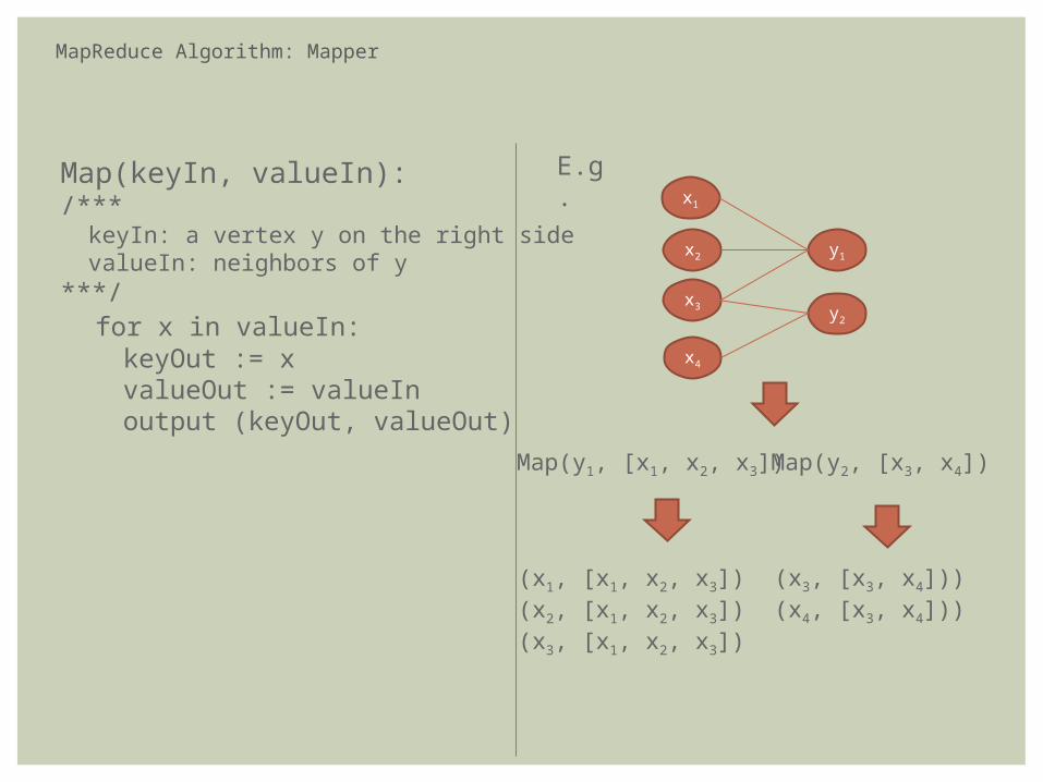
MapReduce Algorithm: Mapper

Map(keyIn, valueIn): /*** keyIn: a vertex y on the right side valueIn: neighbors of y ***/ for x in valueIn: keyOut := x valueOut := valueIn output (keyOut, valueOut)

x1

y1x2

x3

Map(y1, [x1, x2, x3])

(x1, [x1, x2, x3])(x2, [x1, x2, x3])(x3, [x1, x2, x3])

E.g.

y2

x4

Map(y2, [x3, x4])

(x3, [x3, x4]))(x4, [x3, x4]))

MapReduce Algorithm: Reducer

Reduce(keyIn, valueIn):/*** keyIn: a vertex x on the left side valueIn: [ neighbors(y)) | yneighbors(keyIn)]

***/ for neighbors(y) in valueIn: for x’ in neighbors(y): COUNTER[x’] += 1 if COUNTER[x’] >= *|valueIn|: add x’ to Q_BICLIQUE[keyIn]

x1 y1

x2

x3

Map(y1, [x1, x2])

(x1, [x1, x2])(x2, [x1, x2])

E.g.

y2

Map(y2, [x1, x2])

(x1, [x1, x2])(x2, [x1, x2])

y3

Map(y3, [x1, x3])

(x1, [x1, x3])(x3, [x1, x3])

Reduce(x1, [[x1, x2], [x1, x2], [x1, x3]])Reduce(x2, [[x1, x2], [x1,x2]])Reduce(x3, [[x1, x3]])

Q_BICLIQUE[x1] = {x1, x2}Q_BICLIQUE[x2] = {x1, x2} Q_BICLIQUE[x3] = {x1, x3}

MapReduce Algorithm: Bottleneck

• Experimental results on one hour of web browsing logs

• Input graph size = 180 MB

• Map outputs are too large to shuffle efficiently!!

• Same information is copied and sent multiple times

Map output bytes 36 GB

Outline



Problem


Giraph Algorithm

Experiment results

Conclusions

1. Partition the graph into small groups composed of highly correlated nodes in advance

• Improve data locality

• Reduce unnecessary communication cost and disk I/O

2. Utilize Giraph for efficient graph partitioning

Idea for improvement

Giraph Algorithm Overview

• Three phases:

1. Partitioning (Giraph):

• An iterative algorithm dividing the graph into smaller partitions

• The partitioning algorithm is designed to produce good enough partitions without incurring too many communication efforts

2. Augmenting (MapReduce):

• Extend each partition with its adjacent inter-partition edges

3. Computing (MapReduce):

• Compute quasi-bicliques of augmented partitions in parallel

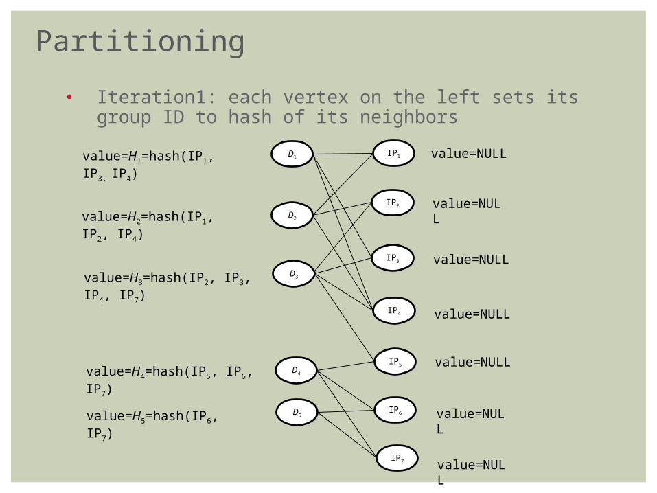
• Iteration1: each vertex on the left sets its group ID to hash of its neighbors

Partitioning

value=H1=hash(IP1, IP3, IP4)


value=H3=hash(IP2, IP3, IP4, IP7)


value=H5=hash(IP6, IP7)

D1

D2

D4

IP1

IP2

IP3

IP5

D5IP6

IP4

IP7

D3

value=NULL

value=NULL

value=NULL

value=NULL

value=NULL

value=NULL

value=NULL

• Iteration2: Each vertex on the right side sets its group ID to the group ID of its highest-degree neighbor.

Partitioning

value=H1

value=H2

value=H3

value=H4

value=H5

D1

D2

D4

IP1

IP2

IP3

IP5

D5IP6

IP4

IP7

D3

value=H1

value=H3

value=H3

value=H3

value=H3

value=H4

value=H4

• Iteration3: Each vertex on the left side changes its group ID to the majority group ID among its neighbors, if any.

Partitioning

value=H3 (changed)

value=H3 (changed)

value=H3

value=H4

value=H4 (changed)

D1

D2

D4

IP1

IP2

IP3

IP5

D5IP6

IP4

IP7

D3

value=H1

value=H3

value=H3

value=H3

value=H3

value=H4

value=H4

• Iteration4: Each vertex on the right side changes its group ID to the majority group ID among its neighbors, if any.

Partitioning

value=H3

value=H3

value=H3

value=H4

value=H4

D1

D2

D4

IP1

IP2

IP3

IP5

D5IP6

IP4

IP7

D3

value=H3

(changed)

value=H3

value=H3

value=H3

value=H3

value=H4

value=H4

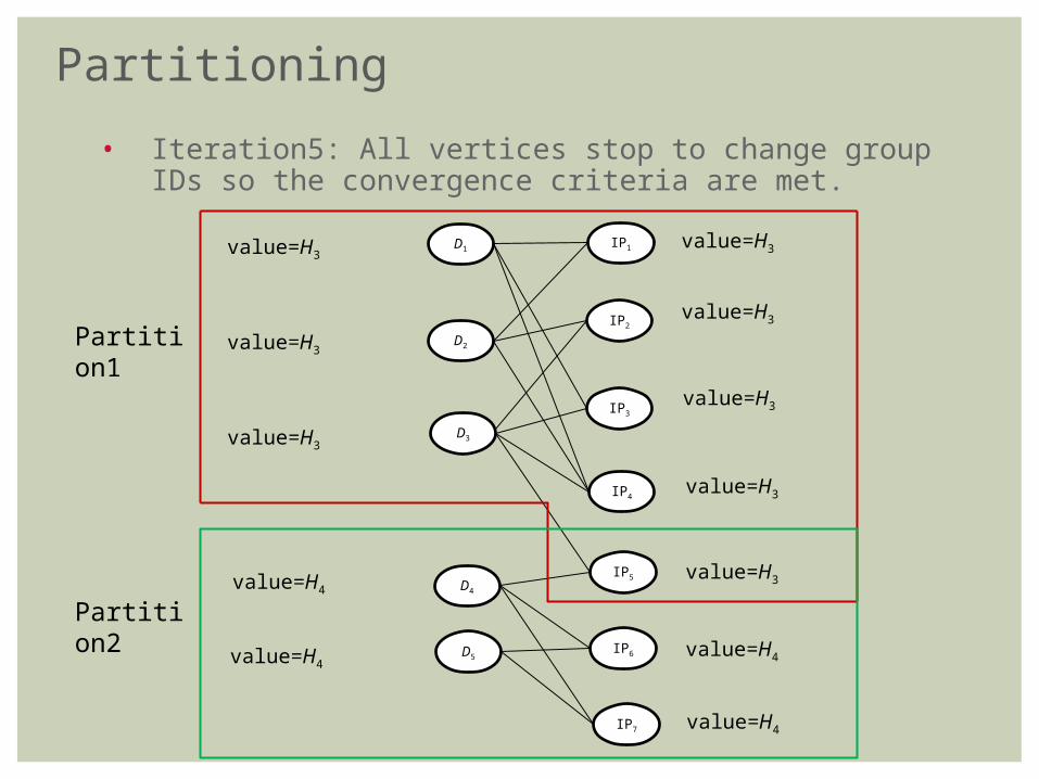
• Iteration5: All vertices stop to change group IDs so the convergence criteria are met.

value=H4

D1

D2

D3

value=H4

value=H3

Partitioning

D4

IP1

IP2

IP3

IP5

D5IP6

IP4

IP7

value=H3

value=H3

value=H3

value=H3

value=H3

value=H3

value=H3

value=H4

value=H4

Partition1

Partition2

Augmenting

D2

D3

D5

IP2

IP3

IP4

IP5

Partition

Augmented partition

IP6

D4

D1

IP1

Computing

Reducer1

augmented partition1


Reducer2



Reducer3



Reducer4



• Compute quasi-bicliques for augmented partitions

• Assign each augmented partition to a reducer

• Each reducer runs a sequential algorithm to compute quasi-bicliques for augmented partitions assigned to it.

Outline



Problem


Giraph Algorithm

Experiment results

Conclusions

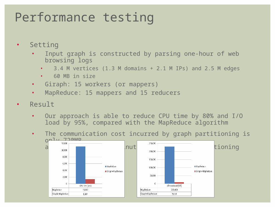
Performance testing

• Setting• Input graph is constructed by parsing one-hour of web browsing logs

• 3.4 M vertices (1.3 M domains + 2.1 M IPs) and 2.5 M edges

• 60 MB in size

• Giraph: 15 workers (or mappers)• MapReduce: 15 mappers and 15 reducers

• Result

• Our approach is able to reduce CPU time by 80% and I/O load by 95%, compared with the MapReduce algorithm

• The communication cost incurred by graph partitioning is only 720MB, and it takes only 1 minute to finish the partitioning

Outline



Problem


Giraph Algorithm

Experiment results

Conclusions

Lessons learned

• Giraph is great for implementing iterative algorithms for it will not bring unnecessary I/O between iterations

• Usecases: Belief propagation, Page Ranking, Random Walk, Connected Componets, Shortest Paths, etc.

• Giraph requires the whole input graph to be loaded into memory

• Proper graph partitioning in advance can significantly improve the performance of following graph mining tasks

• A general graph partitioning algorithm is hard to design for we usually don’t know which nodes should belong to the same group

Future work

• Incremental Graph Mining

• Observe the communication patterns during past incremental mining tasks

• Partition the graph such that nodes which communicate often with each other are in the same group

• Following incremental mining tasks will have lower communication costs

• Consider the situation where the incremental algorithms are hard to design

so the easiest way is to periodically re-compute the result from scratch.

• Pregel: A System for Large-Scale Graph Processing

http://kowshik.github.com/JPregel/pregel_paper.pdf

• Apache Giraph

http://giraph.apache.org/

• GraphLab: A Distributed Framework for Machine Learning in the Cloud

http://vldb.org/pvldb/vol5/p716_yuchenglow_vldb2012.pdf

• Kineograph: Taking the Pulse of a Fast-Changing and Connected World

http://research.microsoft.com/apps/pubs/default.aspx?id=163832

References

Thank You!

Mining quasi bicliques using giraph

Data & Analytics

Transcript of Mining quasi bicliques using giraph