A Distributed Force-Directed Algorithm onGiraph: Design and Experiments∗

Alessio Arleo† Walter Didimo† Giuseppe Liotta†

Fabrizio Montecchiani†

Abstract

In this paper we study the problem of designing a distributed graph visual-ization algorithm for large graphs. The algorithm must be simple to implementand the computing infrastructure must not require major hardware or software in-vestments. We design, implement, and experiment a force-directed algorithm inGiraph, a popular open source framework for distributed computing, based on avertex-centric design paradigm. The algorithm is tested both on real and artificialgraphs with up to million edges, by using a rather inexpensive PaaS (Platform asa Service) infrastructure of Amazon. The experiments show the scalability andeffectiveness of our technique when compared to a centralized implementation ofthe same force-directed model. We show that graphs with about one million edgescan be drawn in less than 8 minutes, by spending about 1$ per drawing in the cloudcomputing infrastructure.

1 IntroductionThe automatic visualization of graphs is a central activity for analyzing and miningrelational data sets, collected and managed through the different kinds of informationsystems and information science technologies. Examples occur in many applicationsdomains, including social sciences, computational biology, software engineering, Webcomputing, information and homeland security (see, e.g., [11, 12, 25, 27, 38, 39]).

Classical force-directed algorithms, like spring embedders, are by far the most pop-ular graph visualization techniques (see, e.g., [11, 28]). One of the key components ofthis success is the simplicity of their implementation and the effectiveness of the re-sulting drawings. Spring embedders and their variants make the final user only a fewlines of code away from an effective layout of a network. They model the graph as aphysical system, where vertices are equally-charged electrical particles that repeal eachother and edges act like springs that give rise to attractive forces. Computing a drawingcorresponds to finding an equilibrium state of the force system by a simple iterativeapproach (see, e.g., [14, 17]).

The main drawback of spring embedders is that they are relatively expensive interms of computational resources, which gives rise to scalability problems even forgraphs with a few thousands vertices. To overcome this limit, sophisticated variants of∗Research supported in part by the MIUR project AMANDA “Algorithmics for MAssive and Networked

DAta”, prot. 2012C4E3KT 001. A preliminary extended abstract of this paper has been accepted to the 23thInternational Symposium on Graph Drawing and Network Visualization (GD’15).†Universita degli Studi di Perugia, Italy, {name.surname}@unipg.it

1

arX

iv:1

606.

0216

2v1

[cs

.DS]

7 J

un 2

016

force-directed algorithms have been proposed; they include hierarchical space parti-tioning, multidimensional scaling, stress-majorization, and multi-level techniques (see,e.g., [3, 18, 20, 28] for surveys and experimental works on these approaches). Also,both centralized and parallel multi-level force-directed algorithms that use the powerof graphical processing units (GPU) have been designed and implemented [19, 24, 37,43]. They scale to graphs with some million edges, but their development requiresa low-level implementation and the necessary infrastructure is typically expensive interms of hardware and maintenance.

Our Contributions Motivated by the increasing availability of scalable cloud com-puting services, we study the problem of designing a simple force-directed algorithmfor a distributed architecture. We want to use such an algorithm on an inexpensivePaaS (Platform as a Service) infrastructure to compute drawings of graphs with millionedges. Our contributions are as follows:

• We give a new distributed force-directed algorithm, based on the Fruchterman-Reingold model [17], designed according to the “Think-Like-A-Vertex (TLAV)”paradigm. TLAV is a vertex-centric approach to design a distributed algorithmfrom the perspective of a vertex rather than of the whole graph. It improveslocality, demonstrates linear scalability, and can be easily adopted to reinterpretmany centralized iterative graph algorithms [31]. Also, it overcomes the limitsof other popular distributed paradigms like MapReduce, which are often poor-performing for iterative graph algorithms [31].

• We describe an implementation and engineering of our algorithm within theApache Giraph framework [9], a popular open-source platform for TLAV dis-tributed graph algorithms. For example, Giraph is used by Facebook to effi-ciently analyze the huge network of its users and their connections [10]. Thecode of our implementation is made available over the Web (http://www.geeksykings.eu/gila/), to be easily re-used in further research on distributedgraph visualization algorithms.

• We present the results of an extensive experimental analysis of our algorithm ona small Amazon cluster of up to 21 computers, each equipped with 4 vCPUs(http://aws.amazon.com/en/elasticmapreduce/). The experiments areperformed both on real and artificial graphs, and show the scalability and effec-tiveness of our technique when compared to a centralized version of the sameforce-directed model. The experimental data also show the very limited cost ofour approach in terms of cloud infrastructure usage. For example, computinga drawing on a set of graphs of our test suite with one million edges requireson average less than 8 minutes, which corresponds to about 1$ (USD) payed toAmazon.

• Finally, we describe an application of our drawing algorithm to visual clusterdetection on large graphs. The algorithm is easily adapted to compute a layoutof the input graph using the LinLog force model proposed by Noack [34], whichis conceived to geometrically emphasize clusters. On this layout, we define andhighlight clusters of vertices by using the K-means algorithm, and experimen-tally evaluate the quality of the computed clustering.

2

Structure of the paper The remainder of the paper is structured as follows. Section 2discussed further work related to our research. Section 3 provides the necessary back-ground on the force-directed model adopted in our solution and on the TLAV paradigmwithin Giraph. In Section 4 we describe in details our distributed algorithm, the re-lated design challenges, and its theoretical computational complexity. In Section 5 wepresent our implementation and the results of our experimental analysis. Section 6shows the application of our algorithm to visual cluster detection on large graphs. Fi-nally, in Section 7 we discuss future research directions for our work.

2 Related WorkSo far, the design of distributed graph visualization algorithms has received limitedattention.

Mueller et al. [33] and Chae et al. [6] proposed force-directed algorithms that usemultiple large displays. Vertices are evenly distributed on the different displays, eachassociated with a different processor, which is responsible for computing the positionsof its vertices; scalability experiments are limited to graphs with some thousand ver-tices. Tikhonova and Ma [40] presented a parallel force-directed algorithm that can runon graphs with few hundred thousand edges. It takes about 40 minutes for a graph of260,385 edges, on 32 processors of the PSC’s BigBen Cray XT3 cluster.

The algorithms mentioned above are mainly parallel algorithms, rather than dis-tributed algorithms. Their basic idea is to partition the set of vertices among the pro-cessors and keep data locality as much as possible throughout the computation.

More recently, Hinge and Auber [23] described a distributed force-directed algo-rithm implemented in the Spark framework (http://spark.apache.org/), usingthe graph processing library GraphX. Their approach is mostly based on a MapReduceparadigm instead of a TLAV paradigm. As for our work, the research of Hinge andAuber goes in the direction of exploring emerging frameworks for distributed graphalgorithms. However, the approach shows margins for improvement: their algorithmtakes 5 hours to compute the layout of a graph with just 8,000 vertices and 35,000edges, on a cluster of 16 machines, each equipped with 24 cores and 48GB of RAM.

3 BackgroundWe first recall the Fruchterman-Reingold force-directed model (Section 3.1), which iscentral for the description of our distributed algorithm. Afterwards, we recall the basicconcepts behind the TLAV paradigm and the Giraph framework (Section 3.2).

3.1 Fruchterman-Reingold Force-Directed AlgorithmTwo main simple principles have guided the design of several force-directed algorithmsover the years (see, e.g., [14, 17]): (i) vertices connected by an edge should be drawnnear to each other; (ii) vertices should not be drawn too close to each other. Wepoint the reader to the comprehensive survey by Kobourov [28] for references andexplanations on the wide literature on this subject. The common ingredients of force-directed algorithms are a model of the physical system of forces acting on the verticesand an iterative algorithm to find a static equilibrium of this system. Here, we restrictour attention to the Fruchterman-Reingold (FR for short) force-directed algorithm [17].

3

According to the FR model, vertices can be viewed as equally-charged electricalparticles and edges act similar to springs; the electrical charges cause repulsion betweenvertices, while the springs cause attraction. Thus, only vertices that are neighbors at-tract each other, but all vertices repel each other. Starting from an initial configura-tion (which usually corresponds to a random placement), the FR algorithm executes asuitable number of iterations, seeking for a static equilibrium of the above defined me-chanical system. In each iteration, the FR algorithm computes the effect of attractiveand repulsive forces on each vertex. The total displacement of a vertex is limited tosome maximum value, which decreases over the iterations. Such a maximum value isoften called the temperature of the system, since its decreasing has the effect of coolingdown the system. Let G = (V,E) be the input graph; the resulting force acting on avertex u ∈ V during each iteration is as follows:

F (u) =∑

(u,v)∈E

fauv(u) +∑

(u,v)∈V×V

fruv(u),

where fauv and fruv denote the attractive force and the repulsive force exerted by von u, respectively. More in detail, denoted by δ(u, v) the Euclidean distance betweenvertices u and v, the absolute values of the forces on u are as follows:

‖fauv‖ =δp(u, v)

d‖fruv‖ =

d2

δq(u, v)

In the above formulas, d is a constant that represents the ideal distance between twovertices, while p and q are two integers that can be suitably tuned based on the struc-ture of the input graphs and on the particular application for which the drawings arecomputed. Clearly, this model is only an approximation of a realistic physical model.In [17] they are chosen such that p = 2 and q = 1 (see also Section 5.1). However,other variants have been proposed such as the one by Noack [34] (see Section 6) .

3.2 The TLAV paradigm and the Giraph frameworkThe vertex-centric programming model is a paradigm for distributed processing frame-works to address computing challenges on large graphs. The idea behind this modelis to “Think-Like-A-Vertex” (TLAV), which translates to implementing distributed al-gorithms from the perspective of a vertex rather than of the whole graph. Each vertexcan store a limited amount of data and can exchange messages only with its neighbors.TLAV frameworks provide a common vertex-centric programming interface, abstract-ing from low-level details of distributed computation, thus improving re-usability andmaintainability of program source codes.

Google’s Pregel [30], based on the Bulk Synchronous Programming model (BSP) [41],was the first published implementation of a TLAV framework. Giraph [9] is a popu-lar TLAV framework built on the Apache Hadoop infrastructure and originated as theopen source counterpart of Pregel. Giraph adds several features to the basic Pregelmodel, although it is still based on the BSP model. In Giraph, the computation is splitinto supersteps executed iteratively and synchronously. A superstep consists of twoprocessing steps:

1. Each vertex executes a user-defined vertex function based on both local vertexdata and on data coming from its adjacent vertices;

4

2. Each vertex sends the results of its local computation to its neighbors, along itsincident edges.

The whole computation ends once a fixed number of supersteps has occurred orwhen certain user-defined conditions are met (i.e., no message has been sent or anequilibrium state is reached). Giraph also allows the definition of global variables(called aggregators), which can be accessed by each vertex during the computation.However, aggregators should be used carefully as they undermine the basic principlesof TLAV and may result in an expensive synchronization cost.

4 A Vertex-Centric Distributed Force-Directed AlgorithmWe first discuss the main challenges that must be addressed in the design a force-directed algorithm for a TLAV framework such as Giraph (Section 4.1). These chal-lenges are mainly related to the calculation of the repulsive forces acting between eachpair of vertices, which requires each vertex to know the positions of all the other ver-tices. After this discussion, we describe our algorithmic solution (Sections 4.2–4.7),based on a pipeline involving several steps of computation.

4.1 Design ChallengesSequential, shared-memory graph algorithms are inherently centralized. They usuallyreceive the entire graph as input, presume all data is accessible in memory, and thegraph is processed in a sequential manner. As already observed, a more local anddistributed approach is more suitable (and often necessary) for processing very largegraphs. Hence, a paradigm shift from centralized to decentralized approaches is neededand, depending on the algorithm, this shift may give rise to some critical challenges.

In the following we discuss the main challenges to be addressed when designing aforce-directed algorithm for a TLAV paradigm. For the sake of presentation, we focuson the FR force-directed algorithm and on the Giraph TLAV framework, although mostof these considerations hold more in general. The following three properties must beguaranteed in the design of a TLAV-based algorithm:

P1. Each vertex exchange messages only with its neighbors;

P2. Each vertex locally stores a small amount of data;

P3. The communication load in each supertsep (i.e., the total number and length ofmessages sent in the superstep) is small: for example, linear in the number ofedges of the graph.

Property P1 usually corresponds to an architectural constraint of the TLAV frame-work. Violating P2 causes out-of-memory errors during the computation of large in-stances. Violating P3 quickly leads to inefficient computations, especially on graphsthat are locally dense or that have high-degree vertices.

Each iteration of the FR algorithm can be directly mapped onto a set of consecutivesupersteps of the computation. Within each iteration, we need to compute the forcesacting on each vertex, which are then used to update the corresponding positions. Re-call that, while attractive forces only act on pairs of adjacent vertices, repulsive forcesact on every pair of vertices. The above three constraints P1–P3 do not allow for sim-ple strategies to make a vertex aware of the positions of all other vertices in the graph,

5

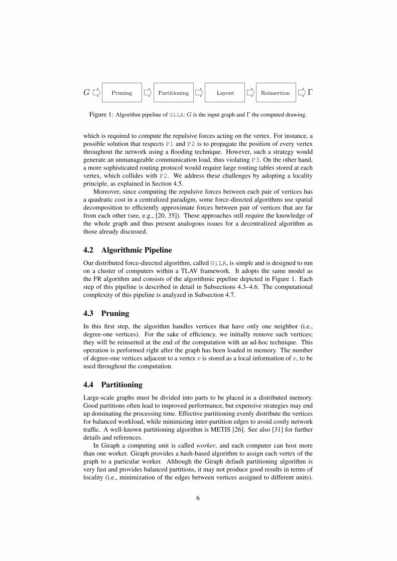
Pruning Partitioning Layout ReinsertionG Γ

Figure 1: Algorithm pipeline of GiLA: G is the input graph and Γ the computed drawing.

which is required to compute the repulsive forces acting on the vertex. For instance, apossible solution that respects P1 and P2 is to propagate the position of every vertexthroughout the network using a flooding technique. However, such a strategy wouldgenerate an unmanageable communication load, thus violating P3. On the other hand,a more sophisticated routing protocol would require large routing tables stored at eachvertex, which collides with P2. We address these challenges by adopting a localityprinciple, as explained in Section 4.5.

Moreover, since computing the repulsive forces between each pair of vertices hasa quadratic cost in a centralized paradigm, some force-directed algorithms use spatialdecomposition to efficiently approximate forces between pair of vertices that are farfrom each other (see, e.g., [20, 35]). These approaches still require the knowledge ofthe whole graph and thus present analogous issues for a decentralized algorithm asthose already discussed.

4.2 Algorithmic PipelineOur distributed force-directed algorithm, called GiLA, is simple and is designed to runon a cluster of computers within a TLAV framework. It adopts the same model asthe FR algorithm and consists of the algorithmic pipeline depicted in Figure 1. Eachstep of this pipeline is described in detail in Subsections 4.3–4.6. The computationalcomplexity of this pipeline is analyzed in Subsection 4.7.

4.3 PruningIn this first step, the algorithm handles vertices that have only one neighbor (i.e.,degree-one vertices). For the sake of efficiency, we initially remove such vertices;they will be reinserted at the end of the computation with an ad-hoc technique. Thisoperation is performed right after the graph has been loaded in memory. The numberof degree-one vertices adjacent to a vertex v is stored as a local information of v, to beused throughout the computation.

4.4 PartitioningLarge-scale graphs must be divided into parts to be placed in a distributed memory.Good partitions often lead to improved performance, but expensive strategies may endup dominating the processing time. Effective partitioning evenly distribute the verticesfor balanced workload, while minimizing inter-partition edges to avoid costly networktraffic. A well-known partitioning algorithm is METIS [26]. See also [31] for furtherdetails and references.

In Giraph a computing unit is called worker, and each computer can host morethan one worker. Giraph provides a hash-based algorithm to assign each vertex of thegraph to a particular worker. Although the Giraph default partitioning algorithm isvery fast and provides balanced partitions, it may not produce good results in terms oflocality (i.e., minimization of the edges between vertices assigned to different units).

6

Recently, Vaquero et al. [42] introduced Spinner, a partitioning algorithm for Giraphbased on iterative vertex migrations, relying only on local information. Starting froma random initial label assignment, which corresponds to an initial partitioning, verticesiteratively adopt the label of the majority of their neighbors until no new labels areassigned (i.e., convergence is reached). On every iteration, each vertex v will make thedecision of either remaining in its current partition set or migrating to a different one.The candidate partition sets for v are those where the highest number of its neighborsare located. Since migrating a vertex potentially introduces a computational overhead,vertex v will preferentially choose to stay in its current partition set if it is one of thecandidates. At the end of the iteration, all vertices that decided to migrate will moveto their desired partition sets. Furthermore, in order to keep the different partition setsbalanced, they have an associated upper capacity. Vertices are allowed to migrate toa different partition set only if its upper capacity has not been yet reached. Vaqueroet al. have shown that partitioning the vertices of the graph by using the Spinneralgorithm speeds up the execution of distributed graph algorithms in the context ofSocial Network Analysis, Mobile Network Communications, and Bioinformatics [42].Based on these experimental findings, we chose to adopt Spinner as partitioningalgorithm for GiLA.

4.5 LayoutThe layout step is the core of GiLA. To execute it, we need to address the challengesdiscussed in Section 4.1. We exploit the experimental evidence that in a drawing com-puted by a force-directed algorithm (see, e.g., [28]):

(a) The graph theoretic distance between two vertices is a good approximation oftheir geometric distance;

(b) The repulsive forces between two vertices u and v tend to be less influential asthe geometric distance between u and v increases.

Based on these two observations, we find it reasonable to adopt a locality principlefor the repulsive forces. Namely, we assume that, for a suitably defined integer con-stant k, the repulsive force acting on each vertex v only depends on its k-neighborhoodNv(k), i.e., the set of vertices whose graph theoretic distance from v is at most k (seealso Figure 2(a)). Clearly, depending on the structure of the graph, small values of kmay affect the accuracy of the forces acting on each vertex. On the other hand, increas-ing k may cause a very high communication load (see Section 4.1); this aspect will bebetter clarified below. Therefore, finding a good trade-off for the value of k is one ofthe main goals of our experimental evaluation (Section 5). We also analyze and discussthe impact of k on the theoretical time complexity of the algorithm (Section 4.7).

The attractive and repulsive forces acting on a vertex are defined according to theFR model (see Section 3.1). In our distributed implementation, each drawing iterationconsists of a sequence of Giraph supersteps and works as follows.

By means of a controlled flooding technique, every vertex v acquires the positionsof all vertices in Nv(k). In the first superstep, v sends a message to its neighbors,which contains the coordinates of v, its unique identifier, and an integer number, calledTTL (Time-To-Live), initially set equal to k (see also Figure 2(b)).

In the second superstep, v processes the received messages and uses them to com-pute the attractive and repulsive forces with respect to its adjacent vertices. Vertexv uses an efficient data structure Hv (a hash set) to store the unique identifiers of its

7

v

(a)

• Sender ID: 1026

• Sender X: 85.2

• Sender Y: 20.4

• TTL: 2

Message

(b)

Figure 2: (a) The 2-neighborhood of a vertex v (white). (b) The structure of a messageused in the Layout phase.

neighbors. Also, it decreases by one unit the TTL of each received message, and for-wards this message to all its neighbors.

In superstep i (i > 2), vertex v processes the received messages and, for eachmessage, v first checks whether the sender u is already present in Hv . If not, v usesthe message to compute the repulsive force with respect to u, and then stores u to Hv .Otherwise, the force exerted by u on v had already been computed in some previoussuperstep. In the first case, v decreases the TTL of the message by one unit and, if it isstill greater than zero, the message is broadcasted to its neighbors; otherwise, v discardsthe message. When no message is sent, the coordinates of each vertex are updated andthe iteration is ended. The amount of messages sent throughout an iteration clearlydepends on k and on the sizes of the k-neighborhoods of the vertices, which is alsorelated to the diameter of the graph.

4.6 ReinsertionOnce a drawing of the pruned graph has been computed, we reinsert the degree-onevertices by means of an ad-hoc technique. The general idea is as follows. For eachvertex v of the pruned graph, we aim at reinserting the degree-one neighbors of v ina geometric neighborhood of v, minimizing the interference with other possible edgesand vertices. Consider the circumference γv centered at v with radius ρ, where ρ issome constant fraction of the length of the shortest edge incident to v. We reinsertthe degree-one neighbors of v by uniformly distributing them along γv , while avoidingedge overlap. We experimentally tuned ρ to 0.2. This reinsertion strategy works fine ifthe disk determined by γv does not contain vertices other than v. In order to enforcethis property as much as possible, the intensity of the repulsive force exerted by v onthe other vertices, during the layout step, is proportional to the number of its degree-oneneighbors.

The pipeline described above is applied independently to each connected compo-nent of the input graph. The layouts of the different components are then convenientlyarranged in a matrix, so to avoid overlap. The pre-processing phase that computesthe connected components of the graph is a distributed adaptation of a classical BFSalgorithm, based on a simple flooding technique.

8

4.7 Teorethical Time ComplexityWe conclude the description of our algorithm with the analysis of its asymptotic worst-case time complexity. An experimental evaluation of the practical running time andscalability of GiLA is presented in Section 5.

Let G be a graph with n vertices and maximum vertex degree ∆. Recall that k isthe integer value used to initialize the TTL of each message. Then the local functioncomputed by each vertex costs O(∆k), since each vertex needs to process (in constanttime) one message for each of its neighbors at distance at most k, and the number ofthese neighbors is O(∆k). Moreover, let c be the number of computing units. Assum-ing that each of them handles (approximately) n/c vertices, we have that each superstepcosts O(∆k)n

c . Let s be the maximum number of supersteps that GiLA performs (ifno equilibrium is reached before), then the time complexity isO(∆k)snc . If we assumethat c and s are constant in the size of the graph, the cost of the algorithm reduces toO(∆k)n, which in the worst case corresponds to O(nk+1).

5 Experimental AnalysisWe conducted an experimental evaluation of our algorithm, GiLA, in terms of qualityof the computed drawings and scalability. We started from the following experimentalhypotheses (expectations):

H1. For small values of k (k ≤ 3), GiLA can draw graphs up to one million edgesin a reasonable time (few minutes), on a cloud computing platform whose usagecost per hour is relatively low. Also, GiLA achieves good performances in termsof weak and strong scalability.

H2. The quality of the drawings computed by GiLA is comparable to that of draw-ings computed by a Fruchterman-Reingold (FR) centralized algorithm, even forrelatively small values of k (3 ≤ k ≤ 4).

H3. For graphs with a relatively small diameter, small increases of k may give rise torelatively high improvements of the drawing quality. Nevertheless, large graphswith a small diameter may cause a dramatic growth of the running time when kis (even slightly) increased.

Hypotheses H1 is motivated by the fact that, for small values of k, the amount ofdata stored at each vertex, as well as the message traffic load, should remain limited.Hypothesis H2 follows from the fact that, for a vertex v and for a relatively small valueof k, most of the vertices that are not in Nv(k) are far from v in the drawing (i.e., thetheoretic distance is a good approximation of the geometric distance). About H3, weexpect that when the diameter of the graph is small, increasing the value of k quicklyleads every Nv(k) to include the majority of the vertices of the graph. This shouldresult in a more accurate computation of the repulsive forces but, at the same time, ina significant growth of the traffic load, and hence of the running time, especially whenthe graph is very large.

The next subsection discusses some details of our implementation, while Sec-tions 5.2 and 5.3 describe the experimental setting and results, respectively.

9

5.1 Implementation DetailsWe implemented GiLA using the version 1.1 of the Giraph framework, and the version2.6 of the Apache Hadoop framework. The source code is publicly available1. In whatfollows, we discuss the implementation and tuning of some salient parameters of thealgorithm. These settings are similar to those used in the centralized implementationof the FR algorithm provided by the Open Graph Drawing Framework (OGDF) [7], awell-known C++ library already used in several applications and experimental works(see, e.g., [3, 8, 22, 32]).

Initially, the vertices of the input graph are randomly placed within a frame of size1200× 1200. In the layout step, the forces acting on each vertex are defined accordingto the FR model (see Section 3.1): the constant d representing the ideal edge lengthis defined as d = Ns +

√N2

h +N2w, where Ns, Nh, and Nw are three constants all

set equal to 20. They correspond, in the displayed visualization, to the ideal distancebetween two vertices (Ns), to the height (Nh) and to the width (Nw) of the graphicfeature representing a vertex (e.g., a rectangle or a circle).

Each computation is halted after a superstep if less than 15% of the vertices has adisplacement larger than 0.01 units. This condition is evaluated using an aggregator(see Section 3.2). Also, the maximum possible displacement for a vertex is computedindependently for each connected component of the graph as follows. Let C be a con-nected component of the input graph G. Let n be the number of vertices of C, and let abe the aspect ratio (i.e., the ratio between the height and the width) of the frame enclos-ing the initial drawing of C. The maximum possible vertex displacement at supersteph is set to dC(h) =

√(nad)0.93h.

5.2 Experimental SettingIn the following we describe: the graph benchmark on which we ran GiLA and a cen-tralized spring embedding algorithm, the metrics adopted to evaluate the performanceof the algorithms, and the distributed infrastructure used for GiLA.

Graph benchmark We used three different benchmarks of graphs:

• Real. It consists of 13 real networks, with up to 1.5 million edges. These graphshave been taken from the Sparse Matrix Collection of the University of Florida2,from the Stanford Large Networks Dataset Collection 3, and from the NetworkData Repository 4 [36]. Details about name, type, and structure of these graphsare reported in Table 1. Previous experiments on the subject use a comparablenumber of real graphs (see, e.g., [40]).

• Synth-Random. It contains 18 synthetic random graphs generated with theErdos-Renyi model [16]. These graphs are divided into six groups of threegraphs each, with size (number of edges)m ∈ {104, 5·104, 105, 106, 1.5·106, 2 ·106} and density (number of edges divided by number of vertices) in the range[2, 3].

1http://www.geeksykings.eu/gila2http://www.cise.ufl.edu/research/sparse/matrices/3http://snap.stanford.edu/data/index.html4http://www.networkrepository.com/

10

NAME |V | |E| DIAMETER DESCRIPTION

add32 4,960 9,462 28 circuit simulation problem

ca-GrQc 5,242 14,496 17 collaboration network

grund 15,575 17,427 15 circuit simulation problem

p2p-Gnutella04 10,876 39,994 9 P2P network

pGp-giantcompo 10,680 48,632 17 email communication network

ca-CondMat 23,133 93,497 14 collaboration network

p2p-Gnutella31 62,586 147,892 11 P2P network

asic-320 121,523 515,300 48 circuit simulation problem

amazon0302 262,111 899,792 32 co-purchasing network

com-amazon 334,863 925,872 44 co-purchasing network

com-DBLP 317,080 1,049,866 21 collaboration network

roadNet-PA 1,087,562 1,541,514 782 road network

Table 1: Details for the Real benchmark. Isolated vertices, self-loops, and parallel edges havebeen removed from the original graphs. The graphs are ordered by increasing number of edges.

• Synth-ScaleFree. It contains 18 synthetic scale-free graphs generated withthe Barabasi-Albert model [2]. Again, these graphs are divided into six groups ofthree graphs each, with size (number of edges) m ∈ {104, 5 · 104, 105, 106, 1.5 ·106, 2 · 106}5 and density in the range [2, 3].

Metrics On each graph of the three benchmarks, we ran GiLA with k ∈ {2, 3, 4}and the (centralized) FR algorithm provided by the Open Graph Drawing Framework(OGDF) [7]. To estimate the resources required by GiLA, we measured for each com-putation both the running time and the cost for using the cloud computing distributedinfrastructure. To estimate the effectiveness of GiLA (i.e., the quality of the computedlayouts), we compared its drawings with those computed by the centralized OGDF al-gorithm, in terms of number of edge crossings, edge length standard deviation, andsimilarity between the “shape” of the drawing and the “structure” of the input graph(see below).

While number of crossings and edge length standard deviation are frequently usedto evaluate the quality of a drawing (see, e.g., [3, 21]), the similarity is a quality metricfor large graphs recently introduced by Eades et al. [15]. The idea behind it is toevaluate the Jaccard sum similarity between the input graph and a proximity graph (inour case the Gabriel Graph) obtained from the set of points representing the verticesin the computed drawing. Briefly, the Jaccard sum similarity measures for each vertexv the number of edges incident to v that are shared by the input graph and by theproximity graph (see [15] for more details). For the sake of presentation, and in orderto compare the different values, we normalized the data between 0 and 1 for each graph.

Distributed infrastructure The experiments on GiLA were executed on the Ama-zon EC2 infrastructure. We experimented three clusters of machines, consisting of10, 15, and 20 machines, respectively. Each machine is a memory-optimized instance

5For each sample m, the actual number of edges of a graph in this sample is approximately m, as thegenerator does not allow to fix the number of edges in a precise way.

11

(a) (b)

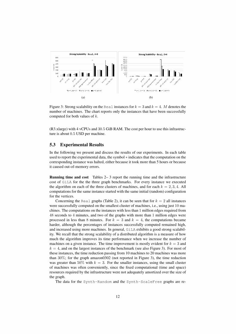
Figure 3: Strong scalability on the Real instances for k = 3 and k = 4. M denotes thenumber of machines. The chart reports only the instances that have been successfullycomputed for both values of k.

(R3.xlarge) with 4 vCPUs and 30.5 GiB RAM. The cost per hour to use this infrastruc-ture is about 0.5 USD per machine.

5.3 Experimental ResultsIn the following we present and discuss the results of our experiments. In each tableused to report the experimental data, the symbol ∗ indicates that the computation on thecorresponding instance was halted, either because it took more than 5 hours or becauseit caused out-of-memory errors.

Running time and cost Tables 2– 3 report the running time and the infrastructurecost of GiLA for the the three graph benchmarks. For every instance we executedthe algorithm on each of the three clusters of machines, and for each k = 2, 3, 4. Allcomputations for the same instance started with the same initial (random) configurationfor the vertices.

Concerning the Real graphs (Table 2), it can be seen that for k = 2 all instanceswere successfully computed on the smallest cluster of machines, i.e., using just 10 ma-chines. The computations on the instances with less than 1 million edges required from48 seconds to 4 minutes, and two of the graphs with more than 1 million edges wereprocessed in less than 8 minutes. For k = 3 and k = 4, the computations becameharder, although the percentages of instances successfully computed remained high,and increased using more machines. In general, GiLA exhibits a good strong scalabil-ity. We recall that the strong scalability of a distributed algorithm is a measure of howmuch the algorithm improves its time performance when we increase the number ofmachines on a given instance. The time improvement is mostly evident for k = 3 andk = 4, and on the largest instances of the benchmark (see also Figure 3). For most ofthese instances, the time reduction passing from 10 machines to 20 machines was morethan 30%; for the graph amazon0302 (not reported in Figure 3), the time reductionwas greater than 50% with k = 3. For the smaller instances, using the small clusterof machines was often conveniently, since the fixed computational (time and space)resources required by the infrastructure were not adequately amortized over the size ofthe graph.

The data for the Synth-Random and the Synth-ScaleFree graphs are re-

12

GiLA- k = 2 GiLA- k = 3 GiLA- k = 4

GRAPH NAME TIME [SEC.] $ TIME [SEC.] $ TIME [SEC.] $

10m

achi

nes

add32 48 0.06 61 0.08 81 0.10ca-GrQc 50 0.06 81 0.10 154 0.19grund 49 0.06 65 0.08 101 0.12p2p-Gnutella04 56 0.07 167 0.21 1051 1.30pGp-giantcompo 52 0.06 90 0.11 185 0.23ca-CondMat 81 0.10 523 0.65 4526 5.58p2p-Gnutella31 75 0.09 217 0.27 3379 4.17asic-320 132 0.31 519 0.64 2245 2.77amazon0302 235 0.09 1703 2.10 ∗ ∗com-Amazon 251 0.29 1079 1.33 ∗ ∗com-DBLP 468 0.16 ∗ ∗ ∗ ∗roadNet-PA 347 0.43 576 0.71 1011 1.25

15m

achi

nes

add32 60 0.11 79 0.14 99 0.18ca-GrQc 61 0.11 91 0.17 142 0.26grund 63 0.11 85 0.15 117 0.21p2p-Gnutella04 67 0.12 130 0.24 643 1.17pGp-giantcompo 66 0.12 100 0.18 173 0.32ca-CondMat 87 0.16 408 0.74 2765 5.03p2p-Gnutella31 74 0.13 211 0.38 1946 3.54asic-320 110 0.20 352 0.64 1622 2.95amazon0302 184 0.34 1011 1.84 ∗ ∗com-amazon 203 0.37 829 1.51 3188 5.80com-DBLP 375 0.68 ∗ ∗ ∗ ∗roadNet-PA 276 0.50 421 0.77 766 1.39

20m

achi

nes

add32 64 0.15 90 0.22 102 0.25ca-GrQc 63 0.15 90 0.22 130 0.31grund 65 0.16 96 0.23 119 0.29p2p-Gnutella04 72 0.17 128 0.31 575 1.38pGp-giantcompo 71 0.17 106 0.26 173 0.42ca-CondMat 88 0.21 341 0.82 1967 4.74p2p-Gnutella31 94 0.23 203 0.49 1623 3.91asic-320 131 0.32 333 0.80 1306 3.15amazon0302 172 0.41 842 2.03 ∗ ∗com-amazon 177 0.43 601 1.45 2653 6.39com-DBLP 364 0.88 4,711 11.35 ∗ ∗roadNet-PA 264 0.64 390 0.94 713 1.72

Table 2: Running time and infrastructure cost for the Real benchmark, on the three types ofclusters.

13

GiLA- k = 2 GiLA- k = 3 GiLA- k = 4

|E| TIME [SEC.] $ TIME [SEC.] $ TIME [SEC.] $10

mac

hine

s10,000 44 0.05 59 0.07 91 0.11

50,000 52 0.06 79 0.10 162 0.20

100,000 60 0.07 111 0.14 381 0.47

1,000,000 205 0.25 751 0.93 ∗ ∗1,500,000 302 0.37 1,293 1.59 ∗ ∗2,000,000 452 0.56 2,088 2.58 ∗ ∗

15m

achi

nes

10,000 54 0.10 70 0.13 97 0.18

50,000 60 0.11 86 0.16 147 0.27

100,000 73 0.13 120 0.22 319 0.58

1,000,000 171 0.31 540 0.98 2,658 4.84

1,500,000 235 0.43 995 1.81 ∗ ∗2,000,000 281 0.51 1,504 2.74 ∗ ∗

20m

achi

nes

10,000 62 0.15 80 0.19 107 0.26

50,000 77 0.18 106 0.26 161 0.39

100,000 90 0.22 134 0.32 286 0.69

1,000,000 167 0.40 447 1.08 2,113 5.03

1,500,000 209 0.50 809 1.95 4,303 10.36

2,000,000 271 0.65 1,154 2.78 ∗ ∗

Table 3: Running time and infrastructure cost for the Synth-Random benchmark achieved onthe three clusters. For each value of |E| we reported the average value on the three graphs with|E| edges.

ported in Table 3 and Table 4, respectively. From the structural point of view, theSynth-Random have a more uniform vertex-degree distribution, while the vertex-degree distribution of the Synth-ScaleFree instances follows a power-law, as theyare scale-free graphs. Clearly, vertices of very high degree may cause a significant workload for GiLA, especially if the graph has a small diameter. Indeed, one can see thatSynth-ScaleFree graphs are the most difficult instances for GiLA: for k ≥ 3, thealgorithm failed the computations on graphs with more than one million edges. Con-versely, GiLA successfully computed all the Synth-Random graphs for k ≤ 3 andsome of the instances for k = 4.

The data about strong scalability on the synthetic graphs confirmed the behavior onthe Real graphs. Figures 4(a), 4(b), and 4(c) summarize these data for k = 2, 3 on theSynth-Random graphs and for k = 2 on the Synth-ScaleFree graphs. Again,augmenting the number of machines does not help when the graphs are relatively small,while it dramatically reduces the running time on the largest instances (of about 40% inthe average). We also report a chart about the weak scalability of GiLA on the syntheticgraphs (see Figure 4(d)). We recall that the weak scalability of a distributed algorithmestimates how the running time varies when we increase the number of machines andthe size of the instances, while keeping the portion of instance handled by each machineconstant. To this aim, we examined the behavior of GiLA for the instances with 106

edges on 10 machines, with 1.5 · 106 edges on 15 machines, and with 2 · 106 edgeson 20 machines. Thus, the number of edges per machine remained approximatelyequal to 100, 000 (since the graphs have a similar density, we can also assume thatthe number of vertices per machine remained approximately the same). In the chart of

14

GiLA- k = 2 GiLA- k = 3 GiLA- k = 4

|E| TIME [SEC.] $ TIME [SEC.] $ TIME [SEC.] $10

mac

hine

s10,000 47 0.06 78 0.10 215 0.26

50,000 58 0.07 227 0.28 1,857 2.29

100,000 77 0.10 603 0.74 4,035 4.98

1,000,000 743 0.92 ∗ ∗ ∗ ∗1,500,000 1,055 1.30 ∗ ∗ ∗ ∗2,000,000 1,689 2.08 ∗ ∗ ∗ ∗

15m

achi

nes

10,000 54 0.10 84 0.15 173 0.32

50,000 70 0.13 185 0.34 1,174 2.14

100,000 87 0.16 398 0.73 2,747 5.00

1,000,000 476 0.87 ∗ ∗ ∗ ∗1,500,000 766 1.39 ∗ ∗ ∗ ∗2,000,000 1,164.00 2.12 ∗ ∗ ∗ ∗

20m

achi

nes

10,000 63 0.15 95 0.23 172 0.41

50,000 76 0.18 180 0.43 915 2.20

100,000 91 0.22 355 0.86 2,112 5.09

1,000,000 403 0.97 ∗ ∗ ∗ ∗1,500,000 571 1.38 ∗ ∗ ∗ ∗2,000,000 956 2.31 ∗ ∗ ∗ ∗

Table 4: Running time and infrastructure cost for the Synth-ScaleFree benchmarkachieved on the three clusters. For each value of |E| we reported the average value on thethree graphs with |E| edges.

(a) (b)

(c) (d)

Figure 4: Strong and weak scalability on the Synth-Random andSynth-ScaleFree instances. M denotes the number of machines.

15

Figure 4(d) we summarize the results for k = 2, for which we have a complete set ofdata. For the Synth-Random graphs, the time increased only by 14 − 15% passingfrom a sample to the next (a constant time value would be the optimum). For theSynth-ScaleFree graphs the time was still rather stable passing from 10 machines(1, 000, 000 vertices) to 15 machines (1, 500, 000 vertices), but it increased of about25% passing from 15 to 20 machines (2, 000, 000 nodes). This suggests that the weakscalability on scale-free graphs is more difficult to predict.

Overall, the results about running time and infrastructure cost seem to largely con-firm H1.

Quality metrics Table 5 reports the quality metrics of GiLA with k = {2, 3, 4}and of the centralized FR algorithm available in the OGDF library (OGDF-FR in thetable). The total number of crossings is divided by the number of edges of the graph,thus indicating the average number of crossings per edge (CRE). Also, for each graph,the series of similarity values (SIM) obtained with the different algorithms and settingshas been normalized and scaled between 0 and 1, so that 1 corresponds to the best valuein the series. We remark that a drawing of the last five largest graphs in this benchmarkcould not be computed neither by GiLA when k = 4 nor by OGDF-FR; hence we donot report the corresponding rows in the table.

We first observe that, for almost all instances, the quality of the drawing in termsof crossings and similarity improves when k increases. Recall that for higher values ofk the computation of the repulsive forces becomes more precise. For all graphs withless than one million edges, the number of crossings per edge is reduced on average by34.5%, while passing from k = 2 to k = 4; also, for k = 4 we get the best similarityvalue in all cases. For the largest graphs these two measures are more stable, althoughwe still observe a crossing reduction of about 27.4% on the graph com-DBLP, whilepassing from k = 2 to k = 3.

Furthermore, on all instances, GiLA with k = 4 behaved better than OGDF-FR interms of number of crossings; the average improvement is about 33.5%. With k = 3,GiLA still produced drawings with less crossings than OGDF-FR in all graphs exceptone, with average improvement of about 23.2%. With k = 2, GiLA caused less cross-ings than OGDF-FR in the 43% of instances (3 over 7). Concerning the similarity,GiLA achieved better values than OGDF-FR in most of the cases, even with k = 2.

About the edge length standard deviation, the values of the drawings computed byGiLA are always smaller than those of the drawings computed by OGDF-FR. However,these values tend to grow when k increases (except for two of the largest graphs, com-amazon and roadNet-PA). Indeed, for k = 2, the edges in the drawing are usuallyshorter than for k = 4, and their length is quite uniform. When k increases, manyedges become longer, due to a broader influence of the repulsive forces.

Figure 5 shows an example of drawings computed by GiLA for the different valuesof k. One can see that the layout is progressively improved while k increases. Thefigure also depicts a drawing of the same graph computed by OGDF-FR. Figure 6shows layouts of the graphs grund and pGp-giantcompo computed by GiLAwith k = 5and by OGDF-FR.

Concerning the synthetic graphs, we have a similar behavior of the quality met-rics (see Tables 6 and 7). In particular, the number of crossings in the drawing ofGiLA is significantly reduced while passing from k = 2 to k = 4, although the finalvalue is closer to that of the drawings computed by OGDF-FR. Also the similarity val-ues usually improve while k is increased and, for k = 4, the values of GiLA on the

16

GiLA- k = 2 GiLA- k = 3

GRAPH NAME CRE ELD SIM CRE ESD SIM

add32 0.07 29.84 0.87 0.07 31.65 0.84

ca-GrQc 1.02 15.04 0.71 0.81 25.93 0.84

grund 0.25 26.75 0.62 0.13 31.99 0.83

p2p-Gnutella04 70.46 15.72 0.26 55.17 35.03 0.65

pgp-giantcompo 1.62 29.28 0.70 1.27 36.88 0.87

ca-CondMat 122.73 18.39 0.39 80.84 42.53 0.51

p2p-Gnutella31 654.09 16.97 0.08 544.16 36.57 0.39

asic-320 74.39 94.45 0.91 75.98 94.06 0.90

amazon0302 2,179.66 52.28 1.00 2,136.00 54.76 0.99

com-amazon 1,012.53 166.06 1.00 1,005.40 165.18 0.99

com-DBLP 10,630.69 49.49 0.94 7,720.00 63.99 1.00

roadNet-PA 911.62 370.86 1.00 913.07 370.95 0.99

GiLA- k = 4 OGDF-FR

GRAPH NAME CRE ELD SIM CRE ELD SIM

add32 0.05 35.84 1.00 0.09 105.62 0.44

ca-GrQc 0.68 41.12 1.00 0.84 80.89 0.78

grund 0.10 44.24 1.00 0.33 182.17 0.04

p2p-gnutella04 52.68 59.71 1.00 62.15 79.27 0.03

pGp-giantcompo 1.13 49.52 1.00 1.87 151.42 0.23

ca-CondMat 64.98 73.37 0.83 78.91 118.74 1.00

p2p-Gnutella31 427.82 73.80 1.00 601.98 148.11 0.04

asic-320 61.60 98.44 1.00 ∗ ∗ ∗com-amazon 1,072.55 155.64 0.97 ∗ ∗ ∗roadNet-PA 910.39 369.54 0.99 ∗ ∗ ∗

Table 5: Average number of crossings per edge (CRE), edge length standard deviation (ELD),and similarity (SIM) for the Real benchmark. For each graph, the similarity values have beennormalized and scaled between 0 and 1, so that 1 corresponds to the best value.

17

(a) (b)

(c) (d)

Figure 5: Drawings of the graph add32 computed by GiLA, with: (a) k = 2, (b) k = 3,and (c) k = 4. The drawing in (d) has been computed by OGDF-FR.

18

(a) grund - GiLA (b) grund - OGDF-FR

(c) pGp-giantcompo - GiLA (d) pGp-giantcompo - OGDF-FR

Figure 6: Drawings of the graphs grund and pGp-giantcompo computed by GiLA withk = 5 and by OGDF-FR.

19

GiLA- k = 2 GiLA- k = 3

|E| CRE ELD SIM CRE ELD SIM

10,000 374.43 9.36 0.37 304.62 17.64 0.72

50,000 1,536.98 8.77 0.56 1,247.99 16.12 0.68

100,000 3,470.94 9.24 0.56 2,833.03 17.43 0.74

1,000,000 29,510.85 8.68 0.87 24,163.59 15.98 0.93

1,500,000 49,665.11 9.09 0.61 40,809.52 17.06 0.93

2,000,000 78,383.53 9.12 0.94 55,913.71 17.18 1.00

GiLA- k = 4 OGDF FR

|E| CRE ELD SIM CRE ELD SIM

10,000 267.89 31.08 1.00 266.77 51.55 0.49

50,000 1,100.38 28.44 1.00 1,066.38 95.94 0.43

100,000 2,518.16 31.83 1.00 2,445.86 114.86 0.44

1,000,000 21,376.95 28.13 1.00 ∗ ∗ ∗1,500,000 32,748.11 28.66 1.00 ∗ ∗ ∗2,000,000 ∗ ∗ ∗ ∗ ∗ ∗

Table 6: Average number of crossings per edge (CRE), edge length standard deviation (ELD),and similarity (SIM) for the Synth-Random graphs. For each graph, the similarity values arenormalized between 0 and 1, so that 1 corresponds to the best value.

Synth-Random graphs are always better than those of OGDF-FR.Overall, the results about the quality metrics are still in favor of hypothesis H2.

We finally observe that also hypothesis H3 seems to be confirmed by the experimentalresults. Indeed, looking at the real instances (for which we have different values of thegraph diameter), the running time is most often negatively affected by small values ofthe diameter when k increases. For the cluster with 10 machines, the graphs for whichwe had the greatest increment of the running time while passing from k = 2 to k = 4are p2p-Gnutella04, ca-CondMat, and p2p-Gnutella31, i.e., those with the smallestdiameter. For the same graphs we observed the highest improvement in the number ofcrossings, together with graph grund, whose diameter is also relatively small. On theopposite, for the graph roadNet-PA, whose diameter is very large, the running time didnot increase too much from k = 2 to k = 4, and the number of crossings improved byonly 0.1%.

6 An Application to Visual Cluster DetectionBig graphs from real-world applications are often small-world networks, locally dense,with an intrinsic community structure. For these graphs, most force-directed algo-rithms, included those based on the classical FR energy model, tend to produce clut-tered drawings with hairball effects, which are not suitable to get detailed informationabout nodes and their connectivity. Instead, there are force-directed layout algorithmsspecifically conceived to give an overview of the graph structure in terms of its clus-ters. Among them, the LinLog energy model proposed by Noack is one of the mostpopular [34].

We applied our distributed force-directed technique to visual cluster detection inbig graphs. Namely, we experimented the following approach: (i) Compute a drawingof the input graph using GiLA with the LinLog energy model in place of the classical

20

GiLA- k = 2 GiLA- k = 3

|E| CRE ELD SIM CRE ELD SIM

10, 000 437.86 14.57 0.03 372.61 30.58 0.17

50, 000 1,634.32 16.36 0.00 1,328.27 37.84 0.24

100, 000 3,250.08 17.47 0.00 2,649.02 42.15 0.08

1, 000, 000 40,811.54 19.47 1.00 ∗ ∗ ∗1, 500, 000 50,803.80 19.24 1.00 ∗ ∗ ∗2, 000, 000 78,383.53 20.10 1.00 ∗ ∗ ∗

GiLA- k = 4 OGDF FR

|E| CRE ELD SIM CRE ELD SIM

10, 000 336.41 44.74 0.69 345.47 51.77 1.00

50, 000 1,227.78 66.34 0.71 1,235.16 88.32 1.00

100, 000 1,634.81 74.93 0.75 1,967.13 111.51 1.00

1, 000, 000 ∗ ∗ ∗ ∗ ∗ ∗1, 500, 000 ∗ ∗ ∗ ∗ ∗ ∗2, 000, 000 ∗ ∗ ∗ ∗ ∗ ∗

Table 7: Average number of crossings per edge (CRE), edge length standard deviation (ELD),and similarity (SIM) for the Synth-ScaleFree graphs. For each graph, the similarity valuesare normalized between 0 and 1, so that 1 corresponds to the best value.

FR model6; (ii) Apply a K-means algorithm [29] to the set of points correspondingto the node positions (disregarding the edges), in order to compute a suitable set K ofnode clusters. We automatically determine K using a local search in a neighborhoodof the initial value K0 =

√n/2 (where n is the number of nodes), and taking the

value for which the corresponding clustering is the best one according to the Calinski-Harabasz qualitative index [13]. (iii) Each cluster is then assigned a different color,which is used to display its nodes.

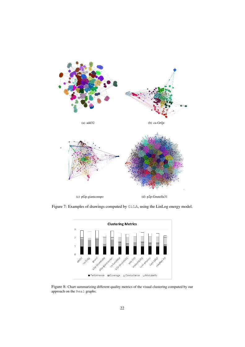
Figure 7 shows examples of visualizations produced with this approach for some ofthe graphs in the Real benchmark. In order to understand whether the visual clustersperceived by the user correspond to good clusters according to the connectivity of thegraph, we measured different widely-used graph clustering quality metrics, namelyperformance, coverage, conductance, and modularity (see, e.g., [1, 4, 5]). The chartin Figure 8 summarizes the values of these metrics for the Real graphs, on whichGiLA ran with the LinLog energy model, with the maximum k for which it succeededto compute a drawing. All values are normalized in the interval [0, 1], where 1 is theoptimum value.

The performance of the clustering is always quite good (close to the optimal value).The conductance (0.57 on average) on the smaller graphs is often low, but it tends toincrease for the larger graphs. The values of coverage (0.55 on average) and modularity(0.51 on average) are more oscillating, but they are still relatively high for severalinstances.

6Observe that the force function deriving from the LinLog energy model can be obtained as a particulartuning of the parameters in the FR force function.

21

(a) add32 (b) ca-GrQc

(c) pGp-giantcompo (d) p2p-Gnutella31

Figure 7: Examples of drawings computed by GiLA, using the LinLog energy model.

Figure 8: Chart summarizing different quality metrics of the visual clustering computed by ourapproach on the Real graphs.

22

7 Conclusions and Future ResearchWe presented GiLA, the first distributed force-directed algorithm running on the Gi-raph framework, which is based on a vertex centric paradigm. Compared to previousparallel and distributed graph layout algorithms, it appears to be faster and more scal-abale to large graphs. We showed that the algorithm can successfully run on an inex-pensive cloud computing platform: layouts of graphs with one million edges can becomputed in few minutes with a cost of few dollars. The code of our implementationis made available over the web.

In the near future, we plan to develop a distributed multi-level force-directed al-gorithm, still based on the TLAV paradigm. The design of such an algorithm is chal-lenging, due to the intrinsic difficulty of efficiently computing the hierarchy requiredby a multi-level approach in a distributed manner, as also observed in [23]. We believethat our TLAV approach can be conveniently exploited to achieve this goal, and thatGiLA can be used as a single-level force-directed algorithm to refine the layouts gen-erated at the different levels of the hierarchy. We recall that multi-level force-directedalgorithms run much faster than single-level ones, and often produce qualitatively bet-ter layouts (see [28] for a high-level description and references about how multi-levelforce-directed algorithms work).

References[1] H. Almeida, D. O. G. Neto, W. M. Jr., and M. J. Zaki. Is there a best quality metric for

graph clusters? In D. Gunopulos, T. Hofmann, D. Malerba, and M. Vazirgiannis, editors,Machine Learning and Knowledge Discovery in Databases - European Conference, ECMLPKDD 2011, Athens, Greece, September 5-9, 2011. Proceedings, Part I, volume 6911 ofLecture Notes in Computer Science, pages 44–59. Springer, 2011.

[2] A.-L. Barabasi and R. Albert. Emergence of scaling in random networks. Science,286(5439):509–512, 1999.

[3] G. Bartel, C. Gutwenger, K. Klein, and P. Mutzel. An experimental evaluation of multilevellayout methods. In U. Brandes and S. Cornelsen, editors, Graph Drawing - 18th Interna-tional Symposium, GD 2010, Konstanz, Germany, September 21-24, 2010. Revised Se-lected Papers, volume 6502 of Lecture Notes in Computer Science, pages 80–91. Springer,2010.

[4] U. Brandes, D. Delling, M. Gaertler, R. Gorke, M. Hoefer, Z. Nikoloski, and D. Wagner.On modularity clustering. IEEE Trans. Knowl. Data Eng., 20(2):172–188, 2008.

[5] U. Brandes, M. Gaertler, and D. Wagner. Engineering graph clustering: Models and exper-imental evaluation. ACM Journal of Experimental Algorithmics, 12:1.1:1–1.1:26, 2007.

[6] S. Chae, A. Majumder, and M. Gopi. Hd-graphviz: Highly distributed graph visualizationon tiled displays. In ICVGIP 2012, pages 43:1–43:8. ACM, 2012.

[7] M. Chimani, C. Gutwenger, M. Junger, G. W. Klau, K. Klein, and P. Mutzel. The opengraph drawing framework (OGDF). In R. Tamassia, editor, Handbook on Graph Drawingand Visualization., pages 543–569. CRC Press, 2013.

[8] M. Chimani, M. Junger, and M. Schulz. Crossing minimization meets simultaneous draw-ing. In IEEE PacificVis 2008, pages 33–40. IEEE, 2008.

[9] A. Ching. Giraph: Large-scale graph processing infrastructure on Hadoop. In HadoopSummit, 2011.

[10] A. Ching, S. Edunov, M. Kabiljo, D. Logothetis, and S. Muthukrishnan. One trillion edges:Graph processing at facebook-scale. PVLDB, 8(12):1804–1815, 2015.

23

[11] G. Di Battista, P. Eades, R. Tamassia, and I. G. Tollis. Graph Drawing. Prentice Hall,Upper Saddle River, NJ, 1999.

[12] W. Didimo and G. Liotta. Mining graph data. In D. J. Cook and L. B. Holder, editors,Graph Visualization and Data Mining, pages 35–64. Wiley, 2007.

[13] R. Dubes. Cluster analysis and related issues. In P. W. C. Chen, L. Pau, editor, Handbook ofPattern Recognition and Computer Vision, pages 3–32. World Scientific, Singapore, 1993.

[14] P. Eades. A heuristic for graph drawing. In Congr. Numerant., volume 42, pages 149–160,1984.

[15] P. Eades, S. Hong, K. Klein, and A. Nguyen. Shape-based quality metrics for large graphvisualization. In E. D. Giacomo and A. Lubiw, editors, Graph Drawing and NetworkVisualization - 23rd International Symposium, GD 2015, Los Angeles, CA, USA, September24-26, 2015, Revised Selected Papers, volume 9411 of Lecture Notes in Computer Science,pages 502–514. Springer, 2015.

[16] P. Erdos and A. Renyi. On random graphs. I. Publicationes Mathematicae, 6:290–297,1959.

[17] T. M. J. Fruchterman and E. M. Reingold. Graph drawing by force-directed placement.Software, Practice and Experience, 21(11), 1991.

[18] H. Gibson, J. Faith, and P. Vickers. A survey of two-dimensional graph layout techniquesfor information visualisation. Information Visualization, 12(3-4):324–357, 2013.

[19] A. Godiyal, J. Hoberock, M. Garland, and J. C. Hart. Rapid multipole graph drawing onthe GPU. In I. G. Tollis and M. Patrignani, editors, GD 2008, volume 5417 of LNCS, pages90–101. Springer, 2009.

[20] S. Hachul and M. Junger. Drawing large graphs with a potential-field-based multilevelalgorithm. In J. Pach, editor, GD 2004, volume 3383 of LNCS, pages 285–295. Springer,2004.

[21] S. Hachul and M. Junger. Large-graph layout algorithms at work: An experimental study.J. Graph Algorithms Appl., 11(2):345–369, 2007.

[22] M. Heiner, M. Herajy, F. Liu, C. Rohr, and M. Schwarick. Snoopy - A unifying petri nettool. In PETRI NETS 2012, volume 7347 of LNCS, pages 398–407. Springer, 2012.

[23] A. Hinge and D. Auber. Distributed graph layout with Spark. In IV 2015, pages 271–276.IEEE, 2015.

[24] S. Ingram, T. Munzner, and M. Olano. Glimmer: Multilevel MDS on the GPU. IEEETrans. Vis. Comput. Graph., 15(2):249–261, 2009.

[25] M. Junger and P. Mutzel, editors. Graph Drawing Software. Springer, 2003.

[26] G. Karypis and V. Kumar. Multilevel graph partitioning schemes. In ICPP 1995, pages113–122. CRC Press, 1995.

[27] M. Kaufmann and D. Wagner, editors. (Eds.) Drawing Graphs. Springer Verlag, 2001.

[28] S. G. Kobourov. Force-directed drawing algorithms. In R. Tamassia, editor, Handbook ofGraph Drawing and Visualization, pages 383–408. CRC Press, 2013.

[29] S. P. Lloyd. Least square quantization in pcm. IEEE Transactions on Information Theory,28(2):129–137, 1982.

[30] G. Malewicz, M. H. Austern, A. J. Bik, J. C. Dehnert, I. Horn, N. Leiser, and G. Cza-jkowski. Pregel: A system for large-scale graph processing. In SIGMOD 2010, pages135–146. ACM, 2010.

[31] R. R. McCune, T. Weninger, and G. Madey. Thinking like a vertex: a survey of vertex-centric frameworks for large-scale distributed graph processing. ACM Comput. Surv.,1(1):1–35, 2015.

24

[32] C. Muelder and K. Ma. Rapid graph layout using space filling curves. IEEE Trans. Vis.Comput. Graph., 14(6):1301–1308, 2008.

[33] C. Mueller, D. Gregor, and A. Lumsdaine. Distributed force-directed graph layout andvisualization. In EGPGV 2006, pages 83–90. Eurographics, 2006.

[34] A. Noack. Energy models for graph clustering. J. Graph Algorithms Appl., 11(2):453–480,2007.

[35] A. J. Quigley and P. Eades. FADE: graph drawing, clustering, and visual abstraction. InGD 2000, volume 1984 of LNCS, pages 197–210. Springer, 2000.

[36] R. A. Rossi and N. K. Ahmed. The network data repository with interactive graph analyticsand visualization. In AAAI 2015, 2015.

[37] P. Sharma, U. Khurana, B. Shneiderman, M. Scharrenbroich, and J. Locke. Speeding upnetwork layout and centrality measures for social computing goals. In J. J. Salerno, S. J.Yang, D. S. Nau, and S. Chai, editors, SBP 2011, pages 244–251. Springer, 2011.

[38] K. Sugiyama. Graph Drawing and Applications for Software and Knowledge Engineers.World Scientific, 2002.

[39] R. Tamassia, editor. Handbook of Graph Drawing and Visualization. CRC Press, 2013.

[40] A. Tikhonova and K. Ma. A scalable parallel force-directed graph layout algorithm. InEGPGV 2008, pages 25–32. Eurographics, 2008.

[41] L. G. Valiant. A bridging model for parallel computation. Commun. ACM, 33(8):103–111,1990.

[42] L. M. Vaquero, F. Cuadrado, D. Logothetis, and C. Martella. Adaptive partitioning forlarge-scale dynamic graphs. In ICDCS 2014, pages 144–153. IEEE, 2014.

[43] E. Yunis, R. Yokota, and A. Ahmadia. Scalable force directed graph layout algorithmsusing fast multipole methods. In ISPDC 2012, pages 180–187. IEEE, 2012.

25