MINING-INDUCED SEISMICITY AND FLAC3D MODELING

AT THE TRAIL MOUNTAIN MINE

by

Meagan Shawn Boltz

A thesis submitted to the faculty of

The University of Utah

in partial fulfillment of the requirements for the degree of

Master of Science

Department of Mining Engineering

The University of Utah

December 2014

Copyright © Meagan Shawn Boltz 2014

All Rights Reserved

The University of Utah Graduate School

STATEMENT OF THESIS APPROVAL

The following faculty members served as the supervisory committee chair and

members for the thesis of Meagan Shawn Boltz .

Dates at right indicate the members’ approval of the thesis.

Michael K. McCarter , Chair _____08/11/14____ Date Approved

Kristine L. Pankow , Co-Chair _____08/11/14____ Date Approved

Zavis M. Zavodni , Member _____08/11/14____ Date Approved

The thesis has also been approved by Michael G. Nelson _

Chair of the Department/School/College of Mining Engineering _

and by David B. Kieda, Dean of The Graduate School.

ABSTRACT

Mining-induced seismicity (MIS) is unpredictable and has the potential to be

damaging; therefore, it is important to study it to gain insight into how rock damage

develops in a mine. A dataset of 1906 mining-induced events was recorded at the Trail

Mountain Mine (TMM). These events cluster on Panel 13, the active panel during data

collection. In this thesis, a FLAC3D

model of the mine was developed to determine if

there are correlations between the seismicity and selected parameters from the model.

A model of a single longwall panel indicates that stresses in the model have an

error of approximately 12.5% due to limitations in the approach used to represent joints.

Subsidence in the model closely matches the subsidence measured at the mine, indicating

that the model captures the first-order behavior of the mine. High stress areas in the

model occur on the gateroads with increasing stress toward the east side of the workings.

Peaks in the maximum shear stress are followed by peaks in seismic moment, which is

consistent with seismicity accompanying de-stressing in the rock mass. Some features of

the seismicity could not be explained by the model, such as the cluster at the end of the

panel, which is thought to have been caused by factors that were not included in the

model. The model also cannot account for the absence of floor events. The reason for

the difference is unclear, but it indicates that stresses alone are not a sufficient indicator

of the potential for MIS. Failed zones in the model were compared with the locations and

moments of the seismicity recorded on Panel 13 and were not found to relate to the

seismicity.

iv

The results of this study indicate that the model is not yet sophisticated enough to

understand the seismicity at the TMM, likely because several features of the mine that

could potentially explain the seismicity, such as near-seam geology and older mine

workings, were not included. This model serves as a foundation for future research on

seismicity at the TMM and provides insight in how to develop similar models for other

mines.

TABLE OF CONTENTS

ABSTRACT.......................................................................................................................iii

LIST OF FIGURES...........................................................................................................vii

ACKNOWLEDGEMENTS................................................................................................ix

1. INTRODUCTION .................................................................................................... 1

1.1. Problem Statement ............................................................................................. 1 1.2. Trail Mountain Setting ....................................................................................... 3

1.2.1. Geology .................................................................................................... 4 1.3. Longwall Mining Method .................................................................................. 6

1.4. Scope of Thesis .................................................................................................. 7

2. RELATING SEISMICITY TO NUMERICAL MODELING ................................ 11

3. FLAC3D MODEL SETUP ..................................................................................... 14

3.1. Grid ................................................................................................................. 14

3.2. Constitutive Behavior ...................................................................................... 15 3.2.1. Rock ........................................................................................................ 15 3.2.2. Coal Seam ............................................................................................... 16

3.2.3. Gob ......................................................................................................... 18 3.3. Material Properties .......................................................................................... 20

3.3.1. Joints ....................................................................................................... 21 3.4. Boundary Conditions ....................................................................................... 26

3.5. Initial Stress State ............................................................................................ 26 3.6. Excavation Sequence ....................................................................................... 27 3.7. Unbalanced Force Ratio .................................................................................. 28

4. SINGLE PANEL TEST MODEL........................................................................... 34

4.1. Stress Propagation During Initial Stress State Calculation ............................. 34 4.2. Stress Concentrations Around the Test Panel .................................................. 35

4.3. Seam Level Displacements .............................................................................. 36 4.4. Calibration to Subsidence Data ....................................................................... 36

4.4.1. Subsidence Data for the Trail Mountain Mine ....................................... 36 4.4.2. Variance Reduction ................................................................................ 37 4.4.3. Subsidence over Panel 5 ......................................................................... 37

5. MINE-WIDE ANALYSIS RESULTS ................................................................... 41

vi

5.1. Subsidence ....................................................................................................... 41 5.2. Failed Zones .................................................................................................... 42 5.3. Vertical Stresses .............................................................................................. 45 5.4. Maximum Shear Stresses ................................................................................. 46

5.5. Change in Maximum Shear Stress ................................................................... 48

6. CONCLUSIONS AND RECOMMENDATIONS ................................................. 59

6.1. Conclusions ..................................................................................................... 59

6.2. Recommendations ........................................................................................... 61

REFERENCES ................................................................................................................. 63

LIST OF FIGURES

FIGURE PAGE

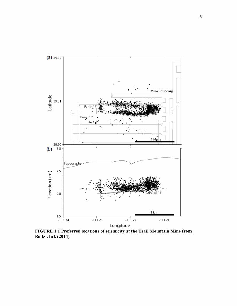
1.1 Preferred locations of seismicity at the Trail Mountain Mine from Boltz et al. (2014) 9

1.2 Stratigraphic column of Trail Mountain ..................................................................... 10

1.3 Diagram of caving developed during longwall mining, after Singh and Kendorski

(1981) ................................................................................................................................ 10

3.1 Grid for the Trail Mountain Mine FLAC3D

model ...................................................... 30

3.2 Map of the Trail Mountain Mine ................................................................................ 31

3.3 Mine geometry represented in the FLAC3D

model...................................................... 31

3.4 Stress vs. strain plot for a 14 m × 14 m × 2.7 m coal pillar with a strength distribution

derived from Karabin and Evanto (1994) ......................................................................... 32

3.5 Comparison of errors for stresses and displacements for different unbalanced force

ratios .................................................................................................................................. 32

4.1 Displacements for Panel 5 at seam level, looking east ............................................... 39

4.2 West to east subsidence profiles from data measured at the mine and recorded in

FLAC3D

after Panel 5 was extracted ................................................................................. 39

4.3 North to south subsidence profiles from data measured at the mine and recorded in

FLAC3D

after Panel 5 was extracted ................................................................................. 40

5.1 West to east subsidence profiles from data measured at the mine and recorded in

FLAC3D

after all panels were extracted ............................................................................ 52

5.2 North to south subsidence profiles from data measured at the mine and recorded in

FLAC3D

after all panels were extracted ............................................................................ 52

5.3 Comparison of (a) the failed zones in the FLAC3D

model and (b) locations of

seismicity recorded during December 2000 in a north to south cross-section ................. 53

5.4 Comparison of the cumulative volume of zones that failed in the FLAC3D

model and

the cumulative seismic moment of events recorded on Panel 13 ..................................... 53

viii

5.5 Plot of vertical stresses around Panels 12 and 13 after all panels were extracted ..... 54

5.6 Vertical stress profiles from west to east on the headgate, tailgate, and center of the

panel at (a) 100 m below mine level, (b) 100 m above mine level, (c) 300 m above mine

level, and (d) at seam level ............................................................................................... 54

5.7 Plot of maximum shear stresses around Panels 12 and 13 after all panels were

extracted ............................................................................................................................ 55

5.8 Maximum shear stress profiles from west to east on the headgate, tailgate, and center

of the panel at (a) 100 m below mine level, (b) 100 m above mine level, (c) 300 m above

mine level, and (d) at seam level ...................................................................................... 55

5.9 Shear stress and seismic moment on the headgate of Panel 13 .................................. 56

5.10 Shear stress and seismic moment on the tailgate of Panel 13 .................................. 56

5.11 Seam-level plots illustrating the change in maximum shear stress caused by the

excavation of material over one-month periods during mining of Panel 13..................... 57

5.12 Cross-section plot illustrating the change in maximum shear stress around Panel 13

........................................................................................................................................... 58

ACKNOWLEDGEMENTS

I would like to thank my advisor, Dr. Michael K. McCarter, for his guidance

during my graduate work and for getting me involved in research. I would also like to

thank Dr. Kristine L. Pankow for her support and mentorship as well as for serving on my

committee. I want to acknowledge Dr. Zavis M. Zavodni for serving on my committee.

I would like to thank Dr. William Pariseau for his mentorship regarding numerical

modeling. I am also grateful for the input from Dr. Keith Koper, Katherine Whidden,

Tex Kubacki, Derrick Chambers, Jessica Wempen, and Jared Stein.

I am grateful to Itasca Consulting Group for allowing me to be a part of their

mentorship program during the course of my research, and I am especially grateful to Dr.

Ed Dzik for serving as my mentor and providing me with valuable advice for working

with FLAC3D

. I would also like to thank Itasca Consulting Group for allowing me access

to their longwall modeling environment.

I thank NIOSH for providing funding for this research (Contract Number 200-

2011-39614) . I thank Energy West Mining Company, a subsidiary of PacifiCorp, for

providing information about the Trail Mountain Mine.

Finally, I would like to thank my family for all of their support during my

schooling as well as the Perkes family for getting me involved in mining engineering and

for all of their support over the years. Thank you also to Ed Bolton for being a friend

when times were tough.

x

The views and conclusions contained in this document are those of the author and

should not be interpreted as representing the opinions or policies of NIOSH or other

supporters of this research.

1. INTRODUCTION

1.1. Problem Statement

Mining-induced seismicity (MIS) has been a prevalent issue in underground coal

mining for many years. MIS is a phenomenon where seismic events occur as a result of

changes in stress and strain in the rock mass due to the excavation of material. Several

factors may influence the generation of MIS, including: geology, depth of cover, in-situ

stress, and mining method (Iannacchione and Zelanko 1995). Seismicity that is directly

related to mining is shallow and often located near mine workings with locations

corresponding to geological and mechanical zones of weakness around the mine

(Johnston 1992). These events are typically small in magnitude (M < 3), and the number

of events is related to mining advance. The seismic activity can be in the form of ground

shaking with no observed damage, or it may consist of violent expulsions of rock, known

as rockbursts or bumps. It is difficult to determine which events are going to be

damaging (Mark 2012); therefore, it is important to study MIS to gain insight into how

rock damage develops in a mine. There has been considerable previous research studying

MIS (see Gibowicz (2009) and Gibowicz and Lasocki (2001) for a review of MIS

research), but exact relations between the mining process and MIS remain largely

unknown.

A dataset was collected by the University of Utah Seismograph Stations at the

Trail Mountain Mine (TMM), which has been extensively studied and relocated (Arabasz

et al. 2002; Arabasz et al. 2005; Boltz et al. 2012; Boltz et al. 2014). Seismicity was

2

recorded from October 2000 to April 2001 at the mine using a temporary seismic array.

While the array was deployed, part of Panel 12 and all of Panel 13 were extracted (Figure

1.1a). Panel 12 was abandoned after excavating 350 m due to excessive seismicity, and

the unmined portion of the panel was left as a barrier between Panel 13 and the older

workings to the south. Approximately 1900 MIS events were recorded at the mine

during the time of the experiment. The events were relocated using multiple techniques

described in Boltz et al. (2014), and the preferred locations for the seismicity are shown

in Figures 1.1a and 1.1b. The locations have good epicentral resolution, with the

seismicity coinciding closely with the mine workings. The locations also have good

hypocentral resolution with the events appearing to occur in the mine roof with depth

errors on the order of several hundred meters. It was not possible to obtain exact

locations for the events; however, the locations are constrained enough to determine

where the seismicity occurs relative to the mine, which can be used to further explore

MIS and its causes.

While locating the MIS at the TMM, it was observed that the seismicity appeared

to cluster on certain areas of Panel 13 (Figure 1.1a). The seismicity clusters along the

gateroads over most of the panel, with the cluster on the tailgate containing more events

than the cluster on the headgate. There is also a significant increase in the number of

events per day (herein referred to as the seismicity rate) at the end of the panel, followed

by the seismicity merging to form a single cluster across the panel. It is hypothesized

that the formation of these clusters may be influenced by areas of high stress

concentration in the mine workings. For instance, the large cluster on the tailgate of

Panel 13 may be due to the tailgate supporting the abutment of older mine workings in

3

addition to Panel 13, despite the presence of a barrier pillar between Panel 13 and these

workings. Factors such as the depth of cover, geology, or the presence of older workings

may have increased stress at the end of the panel and caused the increased seismicity rate.

A recommended method for developing a better understanding of MIS involves

the integration of the analysis of seismic events with numerical modeling (Gibowicz

2009). There have been a growing number of studies that have successfully applied

numerical modeling techniques to longwall mining (e.g., Badr et al. 2003; Maleki 2005;

Pariseau 2012). One common program applied to mining problems is FLAC3D

(Itasca

2013a), a finite difference program developed by the Itasca Consulting Group that is

designed for geotechnical applications. The objective of this study was to develop a

FLAC3D

model of the TMM and determine if there is a correlation between selected

model parameters (failed regions and high stress areas on Panel 13) and the locations of

the MIS.

1.2. Trail Mountain Setting

The TMM is a longwall coal mine with a depth of cover ranging from 430 m to

670 m. Longwall operations were conducted at the mine from October 1995 to April

2001, following room and pillar operations on the east side of the mine. The TMM is

located in the northwestern part of Emery County, Utah, approximately 45 km southwest

of Price, Utah. The mine lies within the Wasatch Plateau coal field and is just east of the

Joes Valley Reservoir. The Wasatch Plateau/Book Cliffs area is one area in the western

United States where MIS is prevalent. Hundreds of mining events are recorded in the

area each year (Ellenberger and Heasley 2000).

4

1.2.1. Geology

The Wasatch Plateau is one of a series of NNE-trending plateaus along the

northwest rim of the Colorado Plateau that correspond to the transition between the Basin

and Range and Colorado Plateau province (Arabasz et al. 2002). The plateau is 145 km

in length in the north-south direction and 11–32 km wide in the east-west direction. The

elevation of the plateau ranges from 1,980 m to 3,350 m (Jones 1994). The Wasatch

Plateau is cut by a series of en echelon north-south trending grabens. The Joes Valley

graben, which lies along the western edge of Trail Mountain, is structurally controlled by

the Joes Valley fault zone, which consists of predominantly north-south striking normal

faults that are nearly parallel to a dominant north-south joint set (Maleki 2005). Trail

Mountain has flat-topped mesas on its upper surface at elevations that range from 2,600

m to greater than 3,000 m. Steep canyon walls resulting from erosional incision of the

Wasatch Plateau form its southern and eastern sides.

Jointing around the TMM is moderately developed with major groups striking

N10°E and N75°W in addition to several minor groups (Jones 1994; Maleki 2005).

Joints are typically near-vertical with lengths of 12–76 m and spacing of 6–122 m

(Maleki 2005). The jointing in the Wasatch Plateau has medium-to-high persistence,

particularly for the north-south oriented set. Joints are mapped in all rock units.

The strata underlying Trail Mountain consist of sedimentary stratigraphic units

that range from upper Cretaceous to Tertiary age and have a shallow westward dip (<5°)

(Arabasz et al. 2002). The strata are made up of sandstones, shales, siltstones,

mudstones, and coal that can be divided into seven major formations, described below

(Figure 1.2).

5

1.2.1.1. Mancos Shale. The Mancos Shale is a massive marine shale. It is

greater than 300 m thick, approaching 395 m near the TMM. Exposed portions of the

shale are soft and well-weathered (Jones 1994).

1.2.1.2. Star Point Sandstone. The Star Point Sandstone is composed of

massive fine-to-medium grained cliff-forming sandstones that are interbedded with the

Mancos Shale and partings of thin-bedded sandstone (Doelling 1972). The unit is 75-106

m thick and is located beneath the shale and mudstone floor of the Hiawatha Coal Seam.

1.2.1.3. Hiawatha Coal Seam. The Hiawatha Coal Seam is the seam that

was mined at the TMM. It is located at the base of the Blackhawk Formation and has

several benches and partings with a mineable thickness of 2.6–4.1 m. The average

mining height at the TMM is 2.7 m. The seam thickness to the north and mudstone

partings near the roof can cause local stability problems to the south (Maleki 2005).

1.2.1.4. Blackhawk Formation. The Blackhawk Formation is 190 m to

245 m thick and contains interbedded layers of siltstones, mudstones, shale, sandstone,

and coal (McCarter and McKenzie 2002). The layers in the Blackhawk Formation

alternate between slope and cliff-forming layers that are less resistant than the

surrounding sandstones. The material above the coal bed consists of braided stream

deposits with lenticular sandstone channels that make up the immediate roof of mineable

coal seams (Doelling 1972).

1.2.1.5. Castlegate Sandstone. The Castlegate Sandstone is a massive

cliff-forming unit that consists of medium-to-coarse grained sandstone with occasional

interbeds of hard shale and conglomerate. The thickness of this unit varies from 52–183

m (McCarter and McKenzie 2002).

6

1.2.1.6. Price River Formation. The Price River Formation is less

resistant to erosion than the Castlegate Sandstone. The formation consists of coarse-

grained sandstones with occasional interbeds of shale, pebble conglomerate, and

mudstone that form step-like outcrops (Doelling 1972). The thickness of this unit ranges

from 183–305 m.

1.2.1.7. North Horn Formation. The North Horn Formation contains

interbeds of sandstone, siltstone, mudstone, and shale with increasing proportions of

limestone near the top of the formation (Jones 1994). The contact between the North

Horn Formation and Price River Formation is not obvious; however, the North Horn

formation is redder and less resistant to erosion and forms slopes and rolling topography

(Doelling 1972).

1.3. Longwall Mining Method

In the longwall mining method, large panels of coal (200–400 m wide, 1–4 km

long, 1.5–6 m tall) are extracted. At the face of the panel, there is a shearer, a conveyor

belt, and a row of shields that span the width of the panel. The shearer cuts the coal

along the width of the panel at the free face. The shields, which separate the shearer and

conveyor from the mined out area, serve to protect the workers and equipment,

temporarily support the immediate roof, control the direction of caving, and walk the

shearer forward. The shearer at the TMM advanced forward an average of 18 m/day. As

the face advances, a void is left in its wake. By design, the roof of the panel caves and

falls into this void, creating what is known as the gob.

The behavior of the roof as the gob is formed is ultimately unknown because it

cannot be directly observed. One accepted description of the behavior in the roof is

7

provided by Singh and Kendorski (1981) and depicted in Figure 1.3. After a sufficient

amount of material is extracted, induced stresses cause the material in the immediate roof

to rubblize and fall into the void. This process progresses upward to approximately three

to six times the mining height. The overlying strata break and slip along existing

discontinuities. The fracturing progresses up another 24 to 54 times the mining height, or

until the broken material bulks enough that overlying strata bend and come to rest on the

gob material, but do not fracture. The bending of successive layers in the roof leads to

the formation of a subsidence trough at the surface.

1.4. Scope of Thesis

The hypothesis of this thesis is that there are correlations between the results of a

numerical model, specifically failed regions and stresses, and the locations and size of

MIS recorded during the mining of Panel 13 at the TMM. In order to carry out this work,

a model featuring the stratigraphy and topography around the TMM was developed using

the finite difference software package, FLAC3D

. The model is based on a longwall

modeling environment previously developed by Itasca Consulting Group (Pierce and

Board 2010). It simulates the caving behavior in a longwall mine using the caving

conceptual model of Singh and Kendorski (1981) and the relationship determined by

Pappas and Mark (1993) to simulate the variation of the elastic modulus of the gob as it is

formed and compacted. A three-dimensional code was selected for the modeling work

because of the significant anisotropy around Panel 13 caused by a large variation in

topography and the influence of old mine workings.

The modeling work was conducted in several steps. The appropriate behavior for

the model was determined and a single longwall panel was excavated to verify that the

8

model functioned as expected. After the model was determined to function properly, a

trial featuring the longwall panels on the west side of the TMM, herein referred to as a

mine-wide analysis, was developed. The older panels were excavated to provide the

initial stress state for Panel 13, as well as to evaluate the subsidence developed in the

model. Panel 13 was then excavated in stages to simulate the advance of the panel. The

accuracy of the model was evaluated by comparing the amount of subsidence generated

in the model with the subsidence data recorded at the mine. A comparison was made

between the failed zones in the model and the seismic moment of events that occurred to

determine if the failed zones can be related to the seismic energy release. Finally, high

stress areas in the mine were identified by examining vertical stress and maximum shear

stress. Correlations between the high stress areas and locations of the seismicity were

explored.

9

FIGURE 1.1 Preferred locations of seismicity at the Trail Mountain Mine from

Boltz et al. (2014)

10

FIGURE 1.2 Stratigraphic column of Trail Mountain

FIGURE 1.3 Diagram of caving developed during longwall mining, after Singh and

Kendorski (1981)

2. RELATING SEISMICITY TO NUMERICAL MODELING

Relating numerical modeling with seismic data is a logical step in furthering the

study of MIS. Currently, there is only limited research on relating these two elements.

This chapter highlights previous methods that have been used to apply numerical

modeling to the study of MIS. These methods include relating the stresses and energy

release in the model to the location and energy of the seismic events.

One method of relating a static numerical model to seismic data is to qualitatively

compare the locations of stress concentrations in the model with the locations of seismic

events. This method has been successfully employed by Senfaute et al. (2001) and

Wilson and Kneisley (1995). In Senfaute et al. (2001), seismic events were recorded at a

longwall coal mine. The mine was modeled using a boundary element method. In their

study, events located close to the area that was being actively mined, and the largest

magnitude events occurred in the high stress areas that were identified in the model.

Wilson and Kneisley (1995) modeled a longwall coal mine in Colorado using the

displacement discontinuity program, MULSIM/PC. They observed that the stress across

the panel face followed a pattern similar to the distribution of energy released by seismic

events at the mine, with increased stress and energy both occurring on the tailgate.

Mercer and Bawden (2005) observed that exploring correlations between stress and

seismicity is a limited method because only weak linear relationships could be found

between the two parameters. Furthermore, they indicate that while identifying high stress

12

areas using seismicity is possible, predicting the potential for seismicity from stresses is

not as straightforward.

In addition to relating stress to seismicity, there are also studies that compare the

energy released in a model with seismicity. Wiles (2005) back-analyzed a series of pillar

bursts at a mine to develop a failure criterion for the energy density in a pillar and used it

to determine whether a failing pillar would produce a rockburst and the amount of energy

that the failure would release. A study by Spottiswoode et al. (2008) examined the

energy release rate (ERR) calculated in models of two South African gold mines. They

observed that the ERR correlates well with a number of seismic parameters, including

number of events, seismic moment, and radiated energy. The ERR is a measure of the

amount of strain energy that is released during failure divided by the area of a mined out

region. An inherent difficulty in using energy to compare seismicity to modeling is that

only a small part (<1%) of the elastic strain energy released during a failure is radiated as

seismic energy (Spottiswoode et al. 2008), which raises the question of whether the total

strain energy can be related to the seismic energy.

Another technique that has been used to relate numerical modeling to MIS is the

excess shear stress (ESS) (Ryder 1987). Prior to the beginning of slip, a plane of

weakness has a static strength that is made up of two parts: the cohesion of the material

and the frictional resistance. After slip begins, the strength of the weakness plane reduces

to a dynamic strength, which is only due to the frictional resistance to sliding. The

reduction in strength results in a stress drop, known as the ESS, which is represented with

the following equation:

(EQ 2.1)

13

where is the shear stress prior to slip, is the normal confining stress, and is the

friction angle. Large values for the ESS (>20 MPa) are indicative of a rupture event.

Maleki (2005) applied excess shear stress (ESS) to an elastic analysis of the TMM to

estimate the locations and magnitudes of events at the mine. He observed that individual

joints in the region were not large enough to produce MIS with magnitudes of the size

observed at the TMM. He instead hypothesized that preexisting weakness planes in the

rock mass could have coalesced to produce a larger discontinuity, which then slipped.

3. FLAC3D MODEL SETUP

The modeling work conducted in this study was conducted with the FLAC3D

software package. It was necessary to use a three-dimensional code for the model

because the region around Panel 13, the panel of interest, is anisotropic due to the

topography and presence of older mine workings. The code used to generate the model is

based on a longwall modeling environment developed by the Itasca Consulting Group

(Pierce and Board 2010), but has been adapted to better suit the conditions at the TMM.

Specifically, changes have been made to incorporate the topography into the

determination of the initial stress state, and logic has been modified to vary the moduli of

zones that have caved. Changes have also been made to the way that joints are

incorporated in the model. This chapter provides details of the structure and constitutive

behavior of the model.

3.1. Grid

The grid for the model consists of the seven stratigraphic layers described in

Section 1.2.1 with an embedded topographic surface (Figure 3.1). The strata around the

TMM dip shallowly (<5°) to the west, but the dip is neglected because it would only have

a small effect on the model results. The zones around the mine workings are evenly

spaced and gradually become larger toward the boundary to reduce the size of the model.

The zones for all layers except the Mancos Shale and Hiawatha Coal Seam are 14 m × 14

m × 14 m. The zones in the Mancos Shale are much coarser at 28 m × 28 m × 78 m, with

15

the longer dimension being in the vertical direction. The zones in the Hiawatha Coal

Seam are 14 m × 14 m × 2.74 m to accommodate the height of the coal seam. The coal

seam is only one element thick to maintain a reasonable model size; therefore, the model

does not capture a detailed stress distribution through the coal seam. Zones surrounding

the topographic surface are refined to more accurately reflect the topography.

A map of the TMM is shown in Figure 3.2. Panels 5–13, the panels on the west

side of the mine, are the workings that are included in the model. Workings on the east

side of the mine were excluded because including them would require doubling the size

of the grid. The grid is too coarse to consider any workings other than the panels

themselves. The mine geometry included in the model is shown in Figure 3.3. Each

panel contains between 380 and 2,480 zones. The workings included in the model cover

a 2,040 m × 2,100 m region. In order to minimize boundary effects, the modeled region

is much larger. The grid is 6,030 m in the east-west direction, 6,280 m in the north-south

direction, and varies in height from 553 m and 1,606 m. There are a total of 7.35 million

zones and 8.40 million gridpoints.

3.2. Constitutive Behavior

The constitutive behavior for the model can be divided into three components: the

behavior of the rock, behavior of the coal seam, and the behavior of the gob. The

behavior is described in the following sections.

3.2.1. Rock

The rock layers above the mine are assigned the built-in Strain-Hardening/

Softening Ubiquitous-Joint (SUBI) constitutive model, which was developed by the

16

Itasca Consulting Group for modeling rock masses. When a zone fails, either the tensile

strength or cohesion of the zone is reduced based on the failure mechanism and strain in

the zone. The residual tensile strength of each zone is set to zero while the residual

cohesion is set to 5% of the intact value. The strain at which the residual value is reached

is based on an empirical relationship determined by Cundall et al. (2005) (from Pierce

and Board 2010):

(EQ 3.1)

where is the residual strain, GSI is the geologic strength index, and ZS is the length

of the sides of the zones in meters, assuming cube-shaped zones. The GSI for the strata

are assumed to be 55. The model results are insensitive to the value used for the residual

strain.

The layer immediately below the mine, the Star Point Sandstone, uses the

Ubiquitous-Joint constitutive model and is unable to soften upon failure. The Mancos

Shale, which is the bottommost layer in the model, is not expected to experience failure

and was assigned an isotropic elastic constitutive model to reduce the size of the model.

3.2.2. Coal Seam

When a coal pillar takes on the load of the mined out area around it, the resulting

stress distribution through the pillar is not uniform. Near the free faces of the pillar, there

is less confinement, causing the strength to be lower. As a result, the coal will fracture

and break off near the faces. Farther into the pillar, the strength of the pillar increases as

the material is under increased confinement and the pillar develops a high-strength core.

17

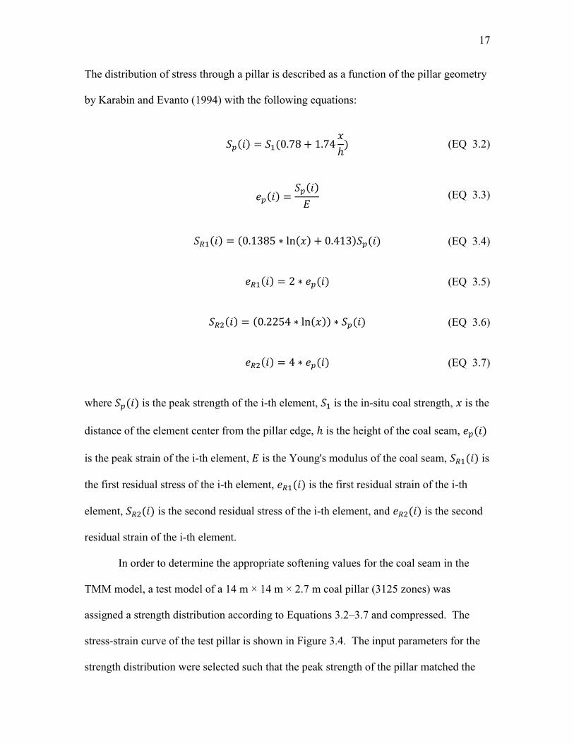
The distribution of stress through a pillar is described as a function of the pillar geometry

by Karabin and Evanto (1994) with the following equations:

(EQ 3.2)

(EQ 3.3)

(EQ 3.4)

(EQ 3.5)

(EQ 3.6)

(EQ 3.7)

where is the peak strength of the i-th element, is the in-situ coal strength, is the

distance of the element center from the pillar edge, is the height of the coal seam,

is the peak strain of the i-th element, is the Young's modulus of the coal seam, is

the first residual stress of the i-th element, is the first residual strain of the i-th

element, is the second residual stress of the i-th element, and is the second

residual strain of the i-th element.

In order to determine the appropriate softening values for the coal seam in the

TMM model, a test model of a 14 m × 14 m × 2.7 m coal pillar (3125 zones) was

assigned a strength distribution according to Equations 3.2–3.7 and compressed. The

stress-strain curve of the test pillar is shown in Figure 3.4. The input parameters for the

strength distribution were selected such that the peak strength of the pillar matched the

18

measured strength of the coal in the Hiawatha coal seam, or 28.5 MPa. As described in

Karabin and Evanto (1994), the pillar behaves elastically up to its peak strength, drops to

a first residual value, and gradually decreases to the second residual value, where the

stress levels off. In this instance, the residual strength is 16.0 MPa, or approximately

56% of the intact strength. The softening behavior seen in Figure 3.4 is applied in the

model by linearly reducing the cohesion after failure to a residual value that is

approximately 56% of the intact cohesion at a strain of 0.045. As with the rock layers, if

a zone in the coal seam fails in tension, it is reduced to zero tensile strength.

3.2.3. Gob

One of the most important aspects of modeling a longwall mine is representation

of the caving behavior. In this model, the caving behavior is simulated according to

Singh and Kendorski (1981) and Pappas and Mark (1993). The behavior is represented

by varying the modulus of gob material as it caves and is recompacted. Additionally,

interfaces are placed between major stratigraphic layers in the roof to allow them to

separate.

When the roof of a mine fails, it caves and falls into the void created by mining

activity. When this occurs, the rock weakens and the modulus of the failed material

drops, causing stress to shed away from the failed area and into the surrounding rock

mass. Later in the caving process, overlying material will also fail or bend and load the

previously failed gob material, recompacting it and causing it to stiffen, which is

represented by an increase in the elastic modulus. The following equation from Salamon

(1990) describes the stress-strain relation for backfill material or aggregates:

19

(EQ 3.8)

where is the vertical stress (compression is positive), is the uncompacted Young's

modulus, is the strain, and is the strain at infinite pressure. Pappas and Mark (1993)

derived an expression for the tangent modulus of an aggregate material by taking the

derivative of Equation 3.8 with respect to the strain. This yields the following equation:

(EQ 3.9)

where is the tangent modulus of the gob material, is the elastic modulus of the

uncompacted caved material, is the vertical stress (compression is positive), and is

the strain at infinite pressure.

The changing modulus of the gob material as it is recompacted is represented with

a routine defined using FLAC3D

's built-in programming language, FISH. When a zone in

the roof fails in tension and falls into the opening created by mining, the elastic modulus

of the zone is reduced to a residual value. The modulus of the zone is then varied using

Equation 3.9 as the zone is gradually reloaded by the overlying zones.

The appropriate values for the uncompacted gob modulus and strain at infinite

pressure were selected to be comparable to literature values and produce subsidence that

matches the subsidence measured at the mine. The values for gob modulus reported in

literature cover a wide range between 7 MPa and 2,000 MPa (Mohamed 2003). The

uncompacted modulus was initially selected as 250 MPa, which was the value used by

Pierce and Board (2010) for their longwall modeling environment. The uncompacted

modulus was increased to 500 MPa, which is still well within the reported range of gob

20

moduli, to better match the mine's subsidence data. The strain at infinite pressure was set

to 0.423, which is the average of the values in Pappas and Mark (1993). The gob

modulus is relatively insensitive to the value selected for the strain at infinite pressure

because the uncompacted modulus is several times larger than the stresses developed in

the failed gob zones.

In addition to recompaction of the gob, interfaces were placed between the

stratigraphic layers in the roof to allow for bending and separation between the layers.

The interfaces obey the Mohr-Coulomb failure criterion and are assigned a friction angle

of 30° and cohesion of zero. The only movement expected along the interfaces is

separation or slip; as a result, the stiffnesses assigned to the interfaces can be set to large

values according to the equation provided by Itasca (2013b).

3.3. Material Properties

Material properties for the roof and floor strata are based on properties presented

in Jones (1994). The compressive strength for the coal seam was taken from a coal pillar

strength study conducted by Pariseau et al. (1977). The properties for the intact rock and

coal are listed in Table 3.1. The friction angle and cohesion were determined from the

unconfined compressive strength and the tensile strength using the following relations:

(EQ 3.10)

(EQ 3.11)

21

where is the friction angle, is the unconfined compressive strength, is the tensile

strength, and is the cohesion.

Material properties testing was conducted on core from a single drill hole located

on the Trail Mountain property after the modeling work was completed. The samples

that were tested were from the Blackhawk Formation and Star Point Sandstone. The

densities of the formations were within 3% of the values used in the model, while the

tensile strengths were approximately double the values used in the model. The difference

between the lab strengths and the strengths used in the model are reasonable because the

samples were dry and only the units that were competent enough to be cut into samples

were included in the testing. The difference in properties would result in changes in

stresses and displacements of less than 10%.

3.3.1. Joints

The strata at the TMM have moderately developed joints with two near-vertical

joint sets, one striking N10°E and one striking N75°W (Jones 1994). There is also a

near-horizontal bedding plane. The presence of jointing in the rock mass must be

accounted for in a numerical model. Jointing can significantly impact the strength of and

cause anisotropy in a rock mass. Jointing also influences the amount and direction of

caving in a caving mine (Sainsbury 2012). There are two ways of representing joints in a

numerical model: explicitly with a discontinuum method and implicitly with an

equivalent continuum. In a discontinuum method, such as the discrete element method,

the rock mass is modeled as intact blocks of rock separated by discontinuities or joints

that are assigned their own strength properties. Explicitly representing joints is

considered to be the most realistic method for representing joints because it allows for the

22

simulation of large displacements and rotations that may occur along the discontinuities

(Kulatilake et al. 2013). Explicitly representing joints can be very computationally

intensive because of the large number of joints that must be represented (Kulatilake et al.

2013).

While an explicit method is a more realistic method of representing joints, it is

possible to obtain reasonable behavior using a scheme that implicitly represents joints

with careful selection of input parameters (Wang et al. 2012). In an implicit or

equivalent continuum method, jointing in the rock mass is represented by adjusting the

material properties of the rock mass such that it behaves as though the joints are present.

Equivalent continuum methods are more common because they are less computationally

intensive and easier to implement.

A variety of methods have been used to represent an equivalent continuum. One

such method is to simply reduce material properties by a set percentage to mimic the

behavior of the jointed rock mass (Wang et al. 2012). Another method treats the joints

and intact rocks as separate materials in a composite and calculates the properties for that

composite, as in the method outlined by Pariseau (2012). The method used by the Itasca

Consulting Group to represent joints is a constitutive model known as the Ubiquitous-

Joint constitutive model and its variation, the SUBI constitutive model (Itasca 2013c).

This constitutive model represents a single weakness plane at a user-specified orientation

in each zone of the model. The strengths and failure criterion of the intact rock and the

joint are treated separately. FLAC3D

first checks for failure of the intact rock and applies

a plastic correction to the stress, if necessary. FLAC3D

then checks for failure of the

23

weakness plane and applies a plastic correction to the stress corresponding to the joint

failure.

One flaw of the Ubiquitous-Joint/SUBI constitutive models is that they use a

nonphysical method of adjusting stresses to account for joint failure. The stress of the

entire zone is adjusted to equal the failure envelope of the weakness plane if failure is

detected in the orientation of the weakness plane. As a result, the stress in the zone may

be biased by the joint, causing the stress to be lower than what would be observed in the

rock mass. This effect becomes more pronounced as zone size increases.

Joints are specified in the TMM model by building a discrete fracture network

(DFN). A DFN is a set of statistical distributions describing the geometrical

characteristics of a set of joints. FLAC3D

generates a set of disk-shaped fractures that

obeys the DFN until some stopping criteria relating to the density of fractures is met. In

the TMM model, the P32 density was used as the stopping criteria for the DFN. The P32

density is the total fracture surface area per unit volume and is related to the persistence

and spacing of a joint set as follows:

(EQ 3.12)

Table 3.2 lists the geometrical properties of the three joint sets. The orientations

of the joints sets are assumed to follow uniform distributions with minimum and

maximum values within ±5° of the reported orientations. The trace lengths are also

assigned a uniform distribution. The measured trace lengths for the area vary from 6.09

m to 76.2 m (Jones 1994; Maleki 2005). The strengths and elastic moduli of the joints

are assumed to be 1% of the intact rock properties. As with the intact rock, the joints

24

soften after failure. Either the cohesion or tension are set to zero depending on whether

the joint fails in shear or tension. The joint friction angles were assigned to be 30°.

The elastic moduli of the joints are not accounted for in FLAC3D

, so an equivalent

Young's modulus and shear modulus were calculated for each zone depending on the

joint set that is applied to the zone. The SUBI model assumes isotropy, so the equivalent

moduli in the vertical direction were assumed to apply to the entire zone, which may not

be an accurate assumption. The joints dip either near-vertically or near-horizontally

(parallel or perpendicular to the loading direction); therefore, simple relationships could

be used to calculate the equivalent moduli (Pariseau 2012). The following equation

describes the equivalent Young's modulus for vertically-dipping joints, which are parallel

to the loading direction:

(EQ 3.13)

where is the equivalent Young's modulus, is the fraction of the zone that is made

up of intact rock, is the Young's modulus of the intact rock, is the fraction of the

zone made up of joints, and is the Young's modulus of the joints. In order to

determine the fraction of the zone that is made up of joint, a joint thickness of 2.54 mm

was assumed. For horizontally-dipping joints, or joints that are perpendicular to the

loading direction, the equivalent Young's modulus may be calculated as follows:

(EQ 3.14)

25

where is the equivalent modulus of the rock, is the equivalent modulus of the joints,

and is the joint spacing. The joint thickness is neglected in this equation. Similar

equations describe the equivalent shear modulus.

After the DFN has been generated and joint properties have been assigned, the

joints are embedded in the model using the SUBI constitutive model. The joint

properties that are assigned to each zone in the model are selected based on which joints

from the DFN intersect the zone. One limitation of the Ubiquitous-Joint and SUBI

constitutive models is that they only account for one plane of weakness per zone. When

multiple joint sets intersect a particular zone, FLAC3D

determines which joint is

represented in the zone based on a user-specified dominance, where the lowest

dominance corresponds to the joint that has the highest priority. If only a small portion

of a lower dominance fracture intersects a zone, the entire zone will take on the properties

of this fracture, even though the fracture should only have a small influence on the zone.

Consequently, the joint set with the lowest dominance may exert an excessive influence

on the model results. Due to the coarse grid size of the TMM model, this effect is even

more pronounced because the zone sizes are larger than the joint spacings, causing the

lowest dominance joint to be present in nearly every zone.

In the model, the horizontal bedding plane is given the lowest dominance, which

is necessary to induce caving. The next lowest dominance is the N10°E joint set, which

is the primary joint set in the Cottonwood Tract (Maleki 2005), followed by the N75°W

joint set. Joints are applied to all layers in the model except the Mancos Shale.

Additionally, the bedding plane is not included in the Hiawatha Coal Seam.

26

3.4. Boundary Conditions

The boundary conditions for the model consist of roller boundaries on the bottom

and sides of the model. The boundary conditions are applied by fixing the displacements

in the direction perpendicular to the side of the model that is constrained. The top of the

model is allowed to remain free.

In order to prevent the overlap of roof and floor zones in the mined-out area, an

interface was applied to the zones in the immediate roof. As with the interfaces between

the roof strata, the interface on the roof zones has a friction angle of 30°, cohesion of

zero, and large stiffness.

3.5. Initial Stress State

The initial stress state is determined in two parts, one to account for the "tectonic

stresses" and one to account for "induced stresses". According to Zoback et al. (1989),

tectonic stresses are made up of the stresses from large-scale, regional forces, while the

induced stresses are those stresses from local effects such as topography, anisotropy, and

effects of erosion. In the tectonic part of the initial stress determination, loading is

assumed to be caused by gravity alone. The model initially consists of a series of

horizontal layers, seen in Figure 3.1a. The vertical stress is assumed to be the maximum

compressive stress and is due to the weight of the rock calculated by:

(EQ 3.15)

where is the vertical stress, is the density of the material, is the gravity constant

(9.81 m/s2), and is the depth to a given point in the model. The horizontal stresses are

equal and are a fraction of the vertical stress, given by:

27

(EQ 3.16)

where is the horizontal stress, is Poisson's ratio, and is the vertical stress. The

average Poisson's ratio of the layers was used. Gravity was applied and the model was

then stepped to equilibrium to adjust the stresses according to the differing material

properties in each layer.

The second part of the initial stress state is the determination of induced changes

due to erosion and the topography. The effects of topography were accounted for in the

model by removing the material above the topographic surface and stepping to

equilibrium (Figure 3.1b). The assumption behind the topography excavation is that the

current topography was reached primarily through erosion of the strata, which is valid in

the region included in the model, and not by tectonic activity.

3.6. Excavation Sequence

The mine workings are excavated in several stages, shown in Figure 3.3. First,

Panels 5–11 are excavated sequentially and the model stepped to equilibrium to provide

the initial stress state for Panels 12 and 13. Next, the mined portion of Panel 12 is

excavated one row of zones at a time (14-m increments) and the model is stepped to

equilibrium after each row. Panel 13 is divided into five pieces, with each piece

representing the monthly production of the panel. As with Panel 12, the five pieces of

Panel 13 are also excavated one row of zones at a time and the model is stepped to

equilibrium after each row. Excavation of the workings is conducted by changing the

28

mechanical model of their zones to null, causing FLAC3D

to ignore them in future

calculations.

3.7. Unbalanced Force Ratio

A major problem with a large numerical model is its associated runtime. When

conducting a mine-wide analysis, it is possible for a single trial to take several days

depending on the computer and the setup of the model. In order to maintain a practical

runtime for the TMM model, adjustments were made to the unbalanced force ratio used

to determine equilibrium. The unbalanced force ratio is the ratio of the average

unbalanced force at all gridpoints in the model to the average applied force at all

gridpoints in the model. By default, FLAC3D

stops cycling when the unbalanced force

ratio reaches 1E-5, which provides high precision results but results in a large runtime. A

larger unbalanced force ratio can be used to reduce the runtime, but there is a tradeoff

between the runtime and the precision in the model that must be considered.

In order to determine the best value for the unbalanced force ratio, a small test

model was built and several trials were conducted with unbalanced force ratios ranging

from 1E-5 to 1E-3. The test model features an excavation that is 648 m long by 252 m

wide (46 × 18 zones) and consists of approximately 392,000 zones. On an HP Z800 with

two Intel Xeon X5687 processors, the runtimes for the model range from 24 to 212

minutes. Figure 3.5 shows a plot comparing the runtime of the test model and the

associated errors for the average vertical stress, seam level displacements, and surface

subsidence relative to an unbalanced force ratio of 1E-5. As the unbalanced force ratio

increases, the runtime decreases and the relative errors rapidly increase, reaching as much

as 90% for an unbalanced force ratio of 1E-3. From the results of this comparison, it was

29

determined that an unbalanced force ratio of 1E-4 is a sufficient ratio for this model. The

ratio provides a significant reduction in runtime, 75 minutes compared to 212 minutes for

the unbalanced force ratio of 1E-5, and increases the error relative to the ratio of 1E-5 by

0.7% for stresses and by 7.8% and 6.4% for seam level displacements and surface

subsidence, respectively.

30

FIGURE 3.1 Grid for the Trail Mountain Mine FLAC

3D model. Upper image shows

all layers of the grid. Lower image shows only layers below the topographic surface.

31

FIGURE 3.2 Map of the Trail Mountain Mine. Hatched areas denote mined-out

regions. Numbers denote the extraction sequence of the panels. Thick dashed lines

denote locations of subsidence profiles. Red rectangle outlines the panels included

in the model. Gray lines show topography.

FIGURE 3.3 Mine geometry represented in the FLAC

3D model

32

FIGURE 3.4 Stress vs. strain plot for a 14 m × 14 m × 2.7 m coal pillar with a

strength distribution derived from Karabin and Evanto (1994)

FIGURE 3.5 Comparison of errors for stresses and displacements for different

unbalanced force ratios

Runtime

Seam Level Displacement

Error

Stress Error

Subsidence Error

0.00%

10.00%

20.00%

30.00%

40.00%

50.00%

60.00%

70.00%

80.00%

90.00%

100.00%

0

50

100

150

200

250

1.00E-05 1.00E-04 1.00E-03

Erro

r

Ru

nti

me

(m

inu

tes)

Unbalanced Force Ratio

Unbalanced Force Error Comparison

33

TABLE 3.1 Intact Rock Properties

Strata Density,

kg/m3

Young's

Modulus,

GPa

Shear

Modulus,

GPa

Unconfined

Compressive

Strength,

MPa

Tensile

Strength,

MPa

North Horn Fm. 2452.9 17.9 7.10 81.4 4.83

Price River Fm. 2291.7 22.1 8.77 68.8 2.62

Castlegate Ss. 2243.6 20.7 8.48 66.1 2.96

Blackhawk Fm. 2484.0 27.6 11.0 108.0 4.96

Hiawatha Coal 1250.0 2.96 1.32 28.5 1.93

Star Point Ss. 2163.5 17.9 7.34 66.4 2.48

Mancos Shale 2323.7 15.2 5.63 - -

TABLE 3.2 Joint Orientation and Spacing

Joint Set Dip Strike Spacing,

m

Maximum Trace,

m Persistence

Set 1 90° N10°E 9.14 76.2 0.6

Set 2 90° N75°W 6.10 76.2 0.6

Set 3 0° - 7.62 76.2 0.6

4. SINGLE PANEL TEST MODEL

Prior to modeling the west block of panels at the TMM, a model consisting of a

single longwall panel was used to verify the behavior of the model as well as to estimate

the error associated with the model. Panel 5 was used as the test panel. This panel was

the first of Panels 5–13 to be extracted, and was the least affected by older mine

workings. Panel 5 was also the only panel from the western block of panels to be mined

in 1997, so subsidence reported in that area that year was only due to Panel 5. Four

aspects of the model were evaluated in this test: the propagation of stresses through the

model, the stress concentrations around the panel, displacements at seam level, and the

subsidence developed over the panel.

4.1. Stress Propagation During Initial Stress State Calculation

Stresses were checked in the coal seam and at the bottom of the model before the

topography was excavated to ensure that the model behaves continuously and stresses

propagate correctly through the model. The stresses were calculated analytically using

Equation 3.15 and Equation 3.16. Table 4.1 compares the analytical stresses with the

FLAC3D

stresses. The error at this stage of the model is acceptable and likely due to an

increased unbalanced force ratio of 1E-4 and numerical error.

35

4.2. Stress Concentrations Around the Test Panel

The stresses at seam level after mining were checked to ensure that the stress

concentrations around the longwall panel are reasonable. This test was repeated twice:

once using just elastic behavior and once using the full constitutive behavior described in

Chapter 3. The stresses in the coal seam after mining were evaluated using the tributary

area formula. The tributary area formula assumes that the stress in the coal seam after

excavation is based on the proportion of material that is removed and is given by:

(EQ 4.1)

where is the stress in the coal seam, is the vertical stress in the coal seam before

mining, and is the extraction ratio, or the area of the mined-out region over the total

area (Pariseau 2007).

The total area used for the extraction ratio is the area of a region that extended

approximately 200 m beyond the longwall panel, or a region that is 1,932 m by 630 m.

The longwall panel is 1,540 m by 224 m, resulting in an extraction ratio of 0.283. The

initial vertical stress in the coal seam is the stress after the topography is excavated. The

initial stress was averaged over the region of interest from the model with elastic

behavior and determined to be 11.3 MPa. The results of this test are also presented in

Table 4.1. The error from the elastic model is fairly small and indicates that stresses are

concentrating correctly around the panel.

The error from the trial with the full constitutive behavior is much larger. The

large error from the model with the full constitutive behavior can be partially attributed to

a combination of the large grid spacing and the way that FLAC3D

handles joints. As

36

described in Section 3.3.1, when a joint is assigned to a zone, the zone is assigned the

strength properties of the joint, but loses the joint dimension. If the joint fails, the stress

of the entire zone is changed, causing the stress to be heavily biased by the joint,

especially if the zone is much larger than the joint.

4.3. Seam Level Displacements

The displacements at seam level were checked to make sure that the interface

between the roof and floor of the test panel prevented them from overlapping. Figure 4.1

shows a plot of the displacement profiles across the panel and their corresponding seam

closure. The roof sag is greater than the floor heave near the gateroads and the floor

heave is slightly greater over the center of the panels. At all points, the seam closure is

less than or equal to the mining height and there are no areas where either the roof sag or

floor heave are excessive. Therefore, this closure check indicates that the interface is

effective in limiting displacements.

4.4. Calibration to Subsidence Data

In order to verify that the results of the model reproduce observations from the

mine, subsidence developed over the workings in the model was compared with

subsidence data reported by the mine.

4.4.1. Subsidence Data for the Trail Mountain Mine

Reports containing subsidence data for the TMM were provided by Energy West

Mining for each year between 1996 and 2002. The data consist of descriptions of the

areas that were mined during the year covered by the reports, contour maps of the

subsidence as determined by aerial survey, and subsidence profiles from west to east and

37

north to south over both the west and southeast panel blocks. The data of interest are the

information for the west panel block for the years 1997 and 2001, which encompass the

first year and last year of extraction of the west block of panels. The subsidence profiles

were compared with those determined in FLAC3D

.

4.4.2. Variance Reduction

The fits between the subsidence profiles recorded at the mine and the profiles

from FLAC3D

were evaluated using the variance reduction. The variance reduction is a

measure of the difference between the magnitude of observed and predicted data

normalized to the magnitude of the observed data (Cohee and Beroza 1994). In this

instance, the data are the amount of subsidence at a given location. The variance

reduction can be determined using the following equation:

(EQ 4.2)

where is the variance reduction, is the measured magnitude of subsidence at

a given point, and is the magnitude of subsidence from FLAC3D

at a given point.

The maximum value of the variance reduction is 100 and it decreases to potentially large

negative numbers as the quality of the fit decreases. For this study, a variance reduction

greater than 75 is considered acceptable.

4.4.3. Subsidence over Panel 5

Panel 5 was selected as the test panel to be used for the subsidence calibration

because it is the first and only panel that was mined from the western block of panels in

1997. As a result, the subsidence measured over this panel is minimally influenced by

38

other mine workings and can be compared to the results of the FLAC3D

model. Three

trials were conducted with different realizations of the DFN to determine the effects that

a different joint distribution would have on the subsidence. The maximum difference

between the three runs was 0.06 m, or about 14%. The subsidence profiles for the three

runs were averaged for comparison with the measured subsidence data.

Figures 4.2 and 4.3 compare the subsidence profiles measured at the mine with

the subsidence recorded by the FLAC3D

model. The variance reduction is calculated over

the gray shaded regions. The subsidence at the mine was not measured beyond these

regions. The magnitudes of the subsidence are similar between the measured and

FLAC3D

profiles, though the model profile is slightly deeper and is more continuous than

the measured data. The widths of the troughs in the FLAC3D

profiles are wider than the

measured data, which may be because the measured data do not include the entire

subsidence trough. The trough is slightly offset between the measured and FLAC3D

north

to south profiles. Variance reductions were calculated as 88.2 from west to east and 82.9

from north to south. Both profiles have variance reductions above 75, and are considered

to be good fits over the regions where the variance reduction was calculated.

39

FIGURE 4.1 Displacements for Panel 5 at seam level, looking east

FIGURE 4.2 West to east subsidence profiles from data measured at the mine and

recorded in FLAC3D

after Panel 5 was extracted. Gray shaded region indicates the

region over which the variance reduction was computed.

40

FIGURE 4.3 North to south subsidence profiles from data measured at the mine and

recorded in FLAC3D

after Panel 5 was extracted. Gray shaded region indicates the

region over which the variance reduction was computed.

TABLE 4.1 Comparison of Analytical and FLAC3D

Stresses

Test Analytical

Value, MPa

FLAC3D

Value, MPa

Error,

%

Vertical Stress, Seam Level 19.3 19.1 1.0

Horizontal Stress, Seam Level 6.11 5.97 2.3

Vertical Stress, Model Base 35.8 34.8 2.9

Horizontal Stress, Model Base 11.3 11.0 2.8

Stress After Excavation, Elastic 15.9 15.3 3.8

Stress After Excavation, Elasto-Plastic 15.9 13.9 12.5

5. MINE-WIDE ANALYSIS RESULTS

The goal of the TMM model is to determine if there are correlations between

features of the model, specifically the failed zones and stresses, and the seismicity

recorded during the mining of Panel 13 at the TMM. In this chapter, the results of the

mine-wide analysis are presented. The subsidence developed in the model is compared

with the subsidence recorded at the mine. Zones that failed during the course of mining

Panel 13 are identified and compared with the locations and seismic moments of the MIS

on Panel 13. Areas of high vertical stress, maximum shear stress, and change in

maximum shear stress are identified and compared with the locations of the seismicity.

5.1. Subsidence

As with the test model from Chapter 4, the subsidence from the mine-wide

analysis was compared with the subsidence recorded at the mine to ensure that the model

reproduces field observations. The subsidence data for the mine from the year 2001 were

used in the comparison. Data were provided for the year 2002, but the data are

inconsistent in that the subsidence decreases by 0.6 m and the mine reported that the data

are suspect. Subsidence profiles are provided for the west-east and north-south directions

in Figures 5.1 and 5.2. The locations of the profiles are marked on Figure 3.2. The west

to east FLAC3D

profile closely matches the data recorded at the mine. The trough reaches

the same depth and is approximately the same width as the mine data, though the

modeled trough is slightly wider. The north to south profile also extends to a similar

42

depth as the measured data. The width of the north to south FLAC3D

trough deviates

from the mine data to the north, likely because the subsidence over Panel 13 was not

measured because it is separated from the other workings. It is also possible that the

subsidence associated with this panel had not fully developed at the time of the survey.

The variance reduction was calculated over the gray shaded regions. The variance

reduction is 96.7 in the west-east direction and 93.2 in the north-south direction. Both

values are well above the cutoff for a good variance reduction.

5.2. Failed Zones

A seismic event occurs when the rock mass fails and radiates energy; therefore, a

relationship might be expected between the failed zones in the model and the MIS

recorded at the mine. The locations of the failed zones in the FLAC3D

model were

compared with the locations of seismic events to determine if the failures coincide with

the seismicity. The seismic moment was also compared with the volume of the failed

zones to determine if there is a relationship between the two parameters. If a relationship

is found, it could indicate that the energy release from the model could be used as a proxy

for potential energy release from seismic events.

Figure 5.3 compares the locations of the failed zones and the locations of the MIS

that was recorded in December 2000. The north-south cross-sections in this figure are

representative of the failed zones and seismicity along the majority of the panel until

reaching the east end, where the seismicity merged across the panel. The failed zones

associated with Panel 13 (Figure 5.3a) consist of tensile failures along the bedding planes

in the immediate roof and floor of the panel surrounded by shearing of joints that extends

approximately 90 m into the roof and 45 m into the floor. The zones around the older

43

mine workings (Panels 5–11) failed in a similar pattern to those around Panel 13.

Additionally, there are zones that have vertical joints that sheared during the initial stress

state determination. The seismicity primarily locates on the gateroads of Panel 13

(Figure 5.3b), with the majority of the events locating in the roof within 250 m of mine

level.

The failed zones in the model occur in different locations than the seismicity.

There are three possible reasons for this difference. First, the model is conducting a static

analysis, so the failure mechanisms in the model do not distinguish between failure that

happens quickly enough to radiate seismic energy and aseismic failure. The second

explanation is related to the failure mechanisms that occur in the model. The failures

occurring directly above and below the workings are predominately tensile failures and

separations along joints, which are expected to release less energy. Tensile failures are

less likely to radiate enough seismic energy to be adequately recorded, which could

explain the lack of observed seismicity over the center of the panel (Luo et al., 1990).

Finally, there is some uncertainty in the locations of the earthquakes, making it difficult

to determine whether failure in a specific zone in the model can be compared to a given

seismic event.

The seismic moment, which is a measure of the energy released by the seismicity

based on the amount of fault slip, can be estimated from the magnitude of an event using

the following empirical equation from Spottiswoode and McGarr (1975):

(EQ 5.1)

44

where is the seismic moment in N-m and is the Richter magnitude. The TMM

coda magnitudes are converted to Richter magnitudes by subtracting 0.44 (Pechmann et

al. 2008). In order to accurately compare the seismic moment with the volume of failed

zones, only events above a magnitude of completeness of 1.1 were included in the

seismic moment calculation.

The volume of the zones that failed around Panel 13 in the model and the seismic

moment of events that were recorded during mining of Panel 13 were tabulated on a

monthly basis. Figure 5.4 compares how the volume of failed zones and the seismic

moment accumulated as the panel progressed. In the FLAC3D

model, the failures

progress at a nearly constant rate as the face advances, resulting in a linear plot for the

cumulative failed volume. The cumulative seismic moment also increased as the panel

progressed, though at a different rate. As with the volume of failed zones, the seismic

moment increases nearly linearly for the first 1060 m of the panel. After this point, the

seismic moment increases more rapidly, corresponding to a more rapid increase in the

seismicity rate. The volume of failed zones does not show this pattern, indicating that it

cannot explain the change in the seismicity rate. This means that the model is either

lacking a feature of the mine that could cause the increase in seismicity, or that the failed

zones are not related to the seismicity. The absence of a relationship between volume of

failed zones and seismic moment is reasonable because there is no spatial relationship

between the failed zones and seismicity. Additionally, the failures in the model do not

distinguish between zones that would fail seismically or aseismically.

45

5.3. Vertical Stresses

In addition to examining failures in the model, the stresses in the model were also

evaluated. Zones of increased vertical stress were identified to determine if there is a

relationship between the stresses and the locations of the seismicity. Figure 5.5 shows

the vertical stresses around Panels 12 and 13 at seam level. The stresses around the edges

of the panels are higher while the stresses over the panels are lower due to excavation.

The area with the greatest vertical stress occurs in the tailgate of Panel 12. Additionally,

the vertical stress increases by 13% in the barrier pillar toward the east end of Panel 13,

where there was an increase in the seismicity rate. The older mine workings also show

an increase in stress toward the east.

Figure 5.6 shows profiles of the vertical stress along the headgate, tailgate, and

center of the panel at varying distances from the mine. The presence of jointing in the

model resulted in large fluctuations in the stress profiles. In order to more clearly

identify trends in the stress, the profiles were smoothed using a moving average with a

100 m window around the point shown on the profile. Within 100 m of the mine, the

stresses on the gateroads are similar in magnitude and greater than the stresses on the

center of the panel. The stress on the panel center is much lower than the gateroad

stresses due to failures in the roof and floor. At 300 m above the workings, the stresses

over the gateroads are similar to the panel center, likely because the roof is not failing at

this distance. The vertical stress gradually increases on the gateroads as the panel

progresses to the east. Additionally, there is a slight dip in stress followed by an increase

in stress, with corresponding fluctuations in the topography, after which the seismicity

merges across the panel.

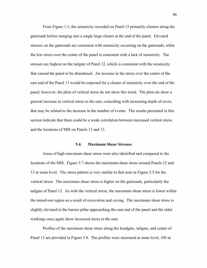
46

From Figure 1.1, the seismicity recorded on Panel 13 primarily clusters along the

gateroads before merging into a single large cluster at the end of the panel. Elevated

stresses on the gateroads are consistent with seismicity occurring on the gateroads, while

the low stress over the center of the panel is consistent with a lack of seismicity. The

stresses are highest on the tailgate of Panel 12, which is consistent with the seismicity

that caused the panel to be abandoned. An increase in the stress over the center of the

east end of the Panel 13 would be expected for a cluster of seismicity over the end of the

panel; however, the plots of vertical stress do not show this trend. The plots do show a

general increase in vertical stress to the east, coinciding with increasing depth of cover,

that may be related to the increase in the number of events. The results presented in this

section indicate that there could be a weak correlation between increased vertical stress

and the locations of MIS on Panels 12 and 13.

5.4. Maximum Shear Stresses

Areas of high maximum shear stress were also identified and compared to the

locations of the MIS. Figure 5.7 shows the maximum shear stress around Panels 12 and

13 at seam level. The stress pattern is very similar to that seen in Figure 5.5 for the

vertical stress. The maximum shear stress is higher on the gateroads, particularly the

tailgate of Panel 12. As with the vertical stress, the maximum shear stress is lower within

the mined-out region as a result of excavation and caving. The maximum shear stress is

slightly elevated in the barrier pillar approaching the east end of the panel and the older

workings once again show increased stress to the east.

Profiles of the maximum shear stress along the headgate, tailgate, and center of

Panel 13 are provided in Figure 5.8. The profiles were measured at seam level, 100 m

47

above and below the mine, and 300 m above the mine. The shear stress profiles were

smoothed using a moving average with a 100 m window around the point shown on the

profile to reduce the stress fluctuations caused by jointing. The maximum shear stress is

higher in the gateroads relative to the center of the panel within 100 m of mine level. At

300 m above the mine, the stress over the gateroads is comparable to the stress over the

center of the panel. The stress is comparable between the headgate and tailgate of the

panel; however, there is a region 100 m above the mine where stress on the tailgate is

significantly higher than stress on the headgate. At seam level, the stress remains

relatively constant along the length of the panel. At other elevations, the gateroad stress

tends to increase to the east, which is most noticeable at elevations other than seam level.

There is a dip in shear stress followed by a significant increase in stress toward the end of

the panel, coinciding with a fluctuation in the topography (Figures 5.9 and 5.10).

Figures 5.9 and 5.10 compare the maximum shear stresses on the gateroads at 100

m into the mine roof with the seismic moment of events that located along the headgate

and tailgate of the panel. The seismic moment was calculated in the same manner as in

Section 5.2. Only the 365 events above a magnitude of completeness of 1.1 were

included. An event was determined to have occurred on the headgate if it was north of

the panel center and on the tailgate if it was south of the panel center. The moment

fluctuates significantly across the panel because there are few events, making it difficult

to identify trends. Additionally, there is some uncertainty in the locations of individual

events. To account for this, the seismic moment was smoothed using a moving average

with a 100 m window. Overall, the shear stress and seismic moment show good

agreement. Areas of the panel that exhibit high shear stress are immediately followed by

48

areas of increased seismic moment as the shear stress decreases. This suggests that the

seismic events accompany the release of energy from the rock mass as it de-stresses.

There is a region of increased seismic moment at the very beginning of the panel that

does not correspond to an area of high shear stress in the model, which is likely due to the

proximity of Panel 13 to Panel 12.

Elevated stresses on the gateroads are consistent with seismicity occurring on the

gateroads. The high shear stress on the tailgate of Panel 12 could be related to the

excessive seismicity that resulted in Panel 12 being abandoned. As with the vertical

stresses, there is not a peak in stress over the center of Panel 13 to indicate that a cluster

would form across the end of the panel. There is a trend of increasing stress as the panel

progresses east, which peaks about 100 m before the seismicity merges across the panel,

supporting the increase in the amount of seismicity at the end of the panel. One

interesting feature of the stresses that is observed with both the vertical stress and the

maximum shear stress is a decrease followed by a significant increase in stress that

coincides with changing topography. The seismicity merges across the panel and the

seismicity rate greatly increases 100 m after this point. This pattern suggests that the

change in topography may be related to the increase in the seismicity rate. Finally, the

region of increased stress on the tailgate between 370 m and 770 m may be related to a

slight increase in seismicity on the tailgate compared to the headgate.

5.5. Change in Maximum Shear Stress

A common method in seismology for evaluating whether stresses are more likely

to promote or inhibit future seismicity is to calculate the Coulomb failure stress change,

given by the following equation:

49

(EQ 5.2)

where is the Coulomb failure stress change, is the change in shear stress along a

weakness plane, is a frictional coefficient, is the change in normal stress along a

weakness plane, and is the change in pore pressure (Stein 1999). The use of Equation

5.2 requires knowledge of the orientation of the plane that slips to generate the future

seismicity, but the failure mechanisms and failure planes are largely unknown for the

TMM dataset. In order to eliminate the need for the failure plane orientation, the change

in maximum shear stress was used as a simplification of this criteria. Seismicity can

occur as a result of relatively small stress changes (Stein 1999), so for this study, a stress

change of 0.1 MPa is considered significant enough to potentially induce seismicity.

Figure 5.11 shows the evolution of the change in maximum shear stress as Panel

13 is mined. Each frame represents the stress change at seam level caused by the

excavation of material during a one-month period. Zones with a positive maximum shear

stress change of greater than 0.1 MPa are shaded, while lower and negative-valued areas

are shown in white. The stress change pattern for each month's excavation is similar.

There are areas of elevated stress changes immediately surrounding the excavation with

smaller stress increases extending approximately one panel-width from the excavation.

As the panel progresses, there is increased stress in the previously mined-out region,

consistent with the recompaction of the gob material as it is loaded by the overburden.

There is also a front abutment stress that extends 28–84 m ahead of the face. The shear

stress changes from the November excavation show positive stress changes around the

mined-out portion of Panel 12 and part of Panel 11 in addition to the stress changes

50

surrounding the mined-out portion of Panel 13. This indicates that there is some

interaction between these workings, which may have influenced the small cluster of

seismicity that occurred at the beginning of mining in Panel 13.

The regions of increased shear stress on the gateroads are consistent with

seismicity occurring on the gateroads, with stress changes being greater on the tailgate.

During the February 2001 excavation, the stresses over the east end of the panel decrease

rather than increase, indicating that the seismicity should not merge across the panel,

despite the locations of the seismicity recorded at the mine. There are two possible

reasons for the cluster not to appear in the model. It is possible that the change in shear

stress alone is not a sufficient indicator of the potential for seismicity. Another

explanation is that the model does not account for some factors that could cause the

cluster. Changes in near-seam geology and the presence of old room-and-pillar workings

to the east of Panel 13 that were not included in the model could influence the stresses at

the east end of the panel and potentially cause seismicity to occur above the panel.

A cross-section of the maximum shear stress change is provided in Figure 5.12.

Areas of high maximum shear stress change occur along the gateroads and the region of

increased stress extends greater than one panel-width on either side of the panel, forming

nearly symmetrical stress lobes. The increased stress persists 300–350 m into both the

roof and floor of the mine. Increased stresses extending into the roof of the mine are

consistent with the extent of the seismicity in the roof. The increased stress in the floor

indicates that there should be an equal amount of seismicity in the roof and floor, though

relatively few events located in the floor (Figure 1.1b). The discrepancy could be

partially caused by a mislocation of the event depths; however, the relative error between

51

events is very small (< 10 m), making it unlikely that the locations could spread enough

to extend 300 m into both the roof and floor. It is also possible that the change in

maximum shear stress alone is not a sufficient indicator of whether or not seismic events

might occur.

52

FIGURE 5.1 West to east subsidence profiles from data measured at the mine and

recorded in FLAC3D

after all panels were extracted. Gray shaded region indicates

the region over which the variance reduction was computed.

FIGURE 5.2 North to south subsidence profiles from data measured at the mine and

recorded in FLAC3D

after all panels were extracted. Gray shaded region indicates

the region over which the variance reduction was computed.

53

FIGURE 5.3 Comparison of (a) the failed zones in the FLAC

3D model and (b)

locations of seismicity recorded during December 2000 in a north to south cross-

section. Black horizontal lines show stratigraphic layering.

FIGURE 5.4 Comparison of the cumulative volume of zones that failed in the

FLAC3D

model and the cumulative seismic moment of events recorded on Panel 13

0

2E+13

4E+13

6E+13

8E+13

1E+14

1.2E+14

1.4E+14

1.6E+14

1.8E+14

2E+14

0

20000

40000

60000

80000

100000

120000

0 500 1000 1500 2000

Cu

mu

lati

ve S

eis

mic

Mo

me

nt

(N-m

)

Cu

mu

lati

ve F

aile

d V

olu

me

(m

3)

Face Advance (m)

Failed Zones

Seismic Moment

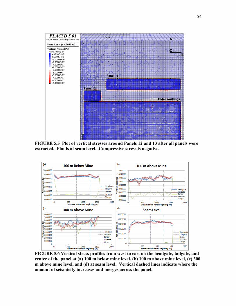
54

FIGURE 5.5 Plot of vertical stresses around Panels 12 and 13 after all panels were

extracted. Plot is at seam level. Compressive stress is negative.

FIGURE 5.6 Vertical stress profiles from west to east on the headgate, tailgate, and

center of the panel at (a) 100 m below mine level, (b) 100 m above mine level, (c) 300

m above mine level, and (d) at seam level. Vertical dashed lines indicate where the

amount of seismicity increases and merges across the panel.

55

FIGURE 5.7 Plot of maximum shear stresses around Panels 12 and 13 after all

panels were extracted. Plot is at seam level.

FIGURE 5.8 Maximum shear stress profiles from west to east on the headgate,

tailgate, and center of the panel at (a) 100 m below mine level, (b) 100 m above mine

level, (c) 300 m above mine level, and (d) at seam level. Vertical dashed lines

indicate where the amount of seismicity increases and merges across the panel.

56

FIGURE 5.9 Shear stress and seismic moment on the headgate of Panel 13

FIGURE 5.10 Shear stress and seismic moment on the tailgate of Panel 13

57

FIGURE 5.11 Seam-level plots illustrating the change in maximum shear stress caused by the excavation of material over one-

month periods during mining of Panel 13. Colored areas denote a positive stress change greater than 0.1 MPa. Dashed lines

delineate the excavation sections for Panel 13.

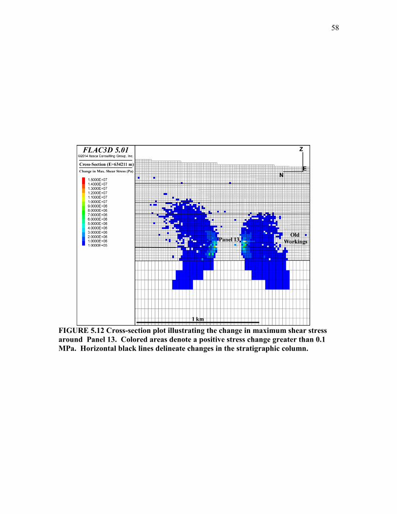
58

FIGURE 5.12 Cross-section plot illustrating the change in maximum shear stress

around Panel 13. Colored areas denote a positive stress change greater than 0.1

MPa. Horizontal black lines delineate changes in the stratigraphic column.

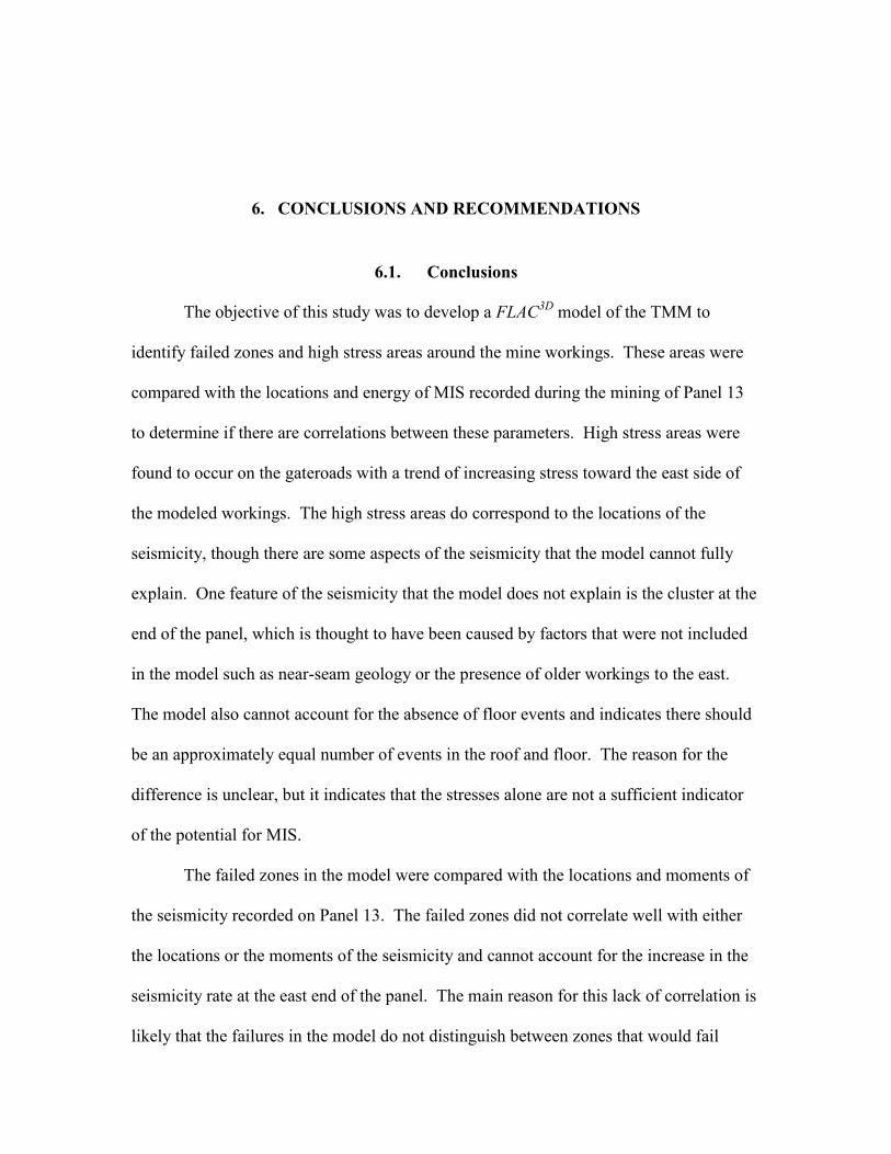
6. CONCLUSIONS AND RECOMMENDATIONS

6.1. Conclusions

The objective of this study was to develop a FLAC3D

model of the TMM to

identify failed zones and high stress areas around the mine workings. These areas were

compared with the locations and energy of MIS recorded during the mining of Panel 13

to determine if there are correlations between these parameters. High stress areas were

found to occur on the gateroads with a trend of increasing stress toward the east side of

the modeled workings. The high stress areas do correspond to the locations of the

seismicity, though there are some aspects of the seismicity that the model cannot fully

explain. One feature of the seismicity that the model does not explain is the cluster at the

end of the panel, which is thought to have been caused by factors that were not included

in the model such as near-seam geology or the presence of older workings to the east.

The model also cannot account for the absence of floor events and indicates there should

be an approximately equal number of events in the roof and floor. The reason for the

difference is unclear, but it indicates that the stresses alone are not a sufficient indicator

of the potential for MIS.

The failed zones in the model were compared with the locations and moments of

the seismicity recorded on Panel 13. The failed zones did not correlate well with either

the locations or the moments of the seismicity and cannot account for the increase in the

seismicity rate at the east end of the panel. The main reason for this lack of correlation is

likely that the failures in the model do not distinguish between zones that would fail

60

seismically or aseismically. It is possible that the relation between these parameters

could be improved by including other factors such as near-seam geology or by better

accounting for the presence of joints.

The maximum shear stress and change in maximum shear stress are the

parameters that were examined in this study that seem to provide the best relation to the

locations of the MIS. The maximum shear stress more clearly illustrates the increasing

stress at the east end of the panel and also shows increased stress on the tailgate relative

to the headgate, consistent with more seismicity on the tailgate. Additionally, the shear

stress lines up with the seismic moment such that areas of increased seismic moment

occur after peaks in the shear stress, which is consistent with the seismicity being related

to de-stressing of the rock mass. The change in maximum shear stress is a useful

parameter because it delineates the extent of stress perturbations caused by the mining

activity. If the events were to have primarily shear failure mechanisms, then it is logical

that the shear stress would be a better indicator of the potential for seismicity.

An inherent flaw with the model developed in this study is the representation of

joints. The SUBI constitutive model uses a nonphysical method for adjusting the stresses

of zones with failed joints, causing an unrealistically low stress in the zone after failure.

The model also does not account for the anisotropy of the elastic moduli as a result of

jointing. The errors introduced by this constitutive model are further compounded by the

use of a coarse grid, causing a single joint set to dominate the model when it should have

a much smaller presence. As a result of the flaws with the representation of joints, the

stresses in zones with joints tend to be lower than reality, causing an error in the stresses

of approximately 12.5%.

61

The results of this thesis are not conclusive enough to predict where seismicity

will occur based on the stresses in the model, but the results are still useful. In addition to

showing that there is a relationship between the stresses and seismicity, the model also

demonstrates that it is possible to conduct a mine-wide analysis using FLAC3D

. A

significant challenge in conducting a mine-wide analysis is that it requires modeling a

large region (6 km × 6 km × 1.5 km) while the coal seam is very thin (< 3 m). This

model illustrates that through careful generation of the grid and selection of the

parameters that define when the model reaches equilibrium, it is possible to obtain both

practical runtimes and reasonable results. The results of the model could also serve as a

foundation for future research on the seismicity at this mine.

6.2. Recommendations

The model presented in this thesis is a good starting point for modeling the MIS

recorded at the TMM. There are a number of ways that this model could be improved in

future work. Factors that are thought to have influenced the seismicity that were not

represented in this model should be included in future modeling efforts. These factors

include changes in near-seam geology, the mine workings located to the east of Panel 13,

and entries around the currently modeled panels.

Another improvement to this model would be the use of a constitutive model that

is better able to account for the presence of jointing in the rock mass. One difficulty with

an equivalent continuum jointing model is being able to accurately reflect the behavior of

the joints. The Ubiquitous-Joint model for FLAC3D

is flawed because it does not account

for anisotropy caused by jointing and it biases the stresses in a zone experiencing joint

failure. There are several models that have been developed that are a step closer to more

62

realistically representing joints in FLAC3D

. One such model is a user-defined constitutive

model for FLAC3D

that accounts for anisotropy in the elastic moduli caused by three

fully-persistent joint sets (Agharazi et al. 2012). This model is still based on the

Ubiquitous-Joint model and has similar problems with nonphysical stress adjustments

after failure. Another alternative could be to use a discontinuum method or to calibrate

the Ubiquitous-Joint model using a discontinuum code (Sainsbury et al. 2008). A finer

grid could also be used to make sure that the different joint sets are adequately

represented.

Finally, future work should focus on examining other parameters that may be

more indicative of the potential for seismicity. While this study and others have shown

that there are weak relationships between shear stress and MIS, the relationships are

insufficient to determine areas in a mine that may be more likely to experience

seismicity. Other parameters that may be better related to seismicity include the excess

shear stress, Coulomb failure stress changes, or energy release in the model.

REFERENCES

Agharazi, A., Martin, C.D., Tannant, D.D. 2012. A three dimensional equivalent

continuum constitutive model for jointed rock masses of up to three joint sets.

Geomechanics and Geoengineering: An Int. J. 7(4): 227–238. Accessed September

2013. doi 10.1080/17486025.2012.714476.

Arabasz, W.J., Nava, S.J., McCarter, M.K., and Pankow, K.L. 2002. Ground Motion

Recording and Analysis of Mining-Induced Seismicity in the Trail Mountain Area,

Emery County, Utah. Final report to State of Utah School and Institutional Trust

Lands Administration. Salt Lake City, UT: University of Utah Seismograph Stations.

Arabasz, W.J., Nava, S.J., McCarter, M.K., Pankow, K.L., Pechmann, J.C., Ake, J., and

McGarr, A. 2005. Coal-mining seismicity and ground-shaking hazard: A case study

in the Trail Mountain area, Emery County, Utah. Bull. Seismol. Soc. Am. 95(1):18–

30. Accessed November 2012. doi 10.1785/0120040045.

Badr, S., Ozbay, U., Keiffer, S., and Salamon, M. 2003. Three-dimensional strain

softening modeling of deep longwall coal mine layouts. In FLAC and Numerical

Modeling in Geomechanics. Lisse: Swets and Zetlinger. pp. 233–239.

Boltz, M. S., Pankow, K.L., and McCarter, M.K. 2012. Relocating mining-induced

seismicity at the Trail Mountain Mine. In Proc. of the 31st Int. Conf. on Ground

Control in Min. Morgantown, WV, July 31–August 2.

Boltz, M.S., Pankow, K.L., and McCarter, M.K. 2014. Fine details of mining-induced

seismicity at the Trail Mountain Mine using modified hypocentral relocation

techniques. Bull. Seismol. Soc. Am. 104(1). Accessed February 2014. doi

10.1785/0120130011.

Cohee, B.P., and Beroza, G.C. 1994. A comparison of two methods for earthquake source

inversion using strong motion seismograms. Annali di Geofisica. 37(6):1515–1538.

Cundall, P., Gomez, P., Lorig, L. Pierce, M., Sainsbury, D., Young, P. and

Napier, P. 2005. Caving Mechanics Task 1 Scoping Study. Report to the

International Caving Study, ICG052292-1-8.

Doelling, H.H. 1972. Central Utah Coal Fields: Sevier-Sanpete, Wasatch Plateau, Book

Cliffs and Emery. Salt Lake City, UT: Utah Geological and Mineralogical Survey.

Ellenberger, J.L., and Heasley, K.A. 2000. Coal mine seismicity and bumps: historical

case studies and current field activity. In Proc. of the 19th Int. Conf. on Ground

64

Control in Min. Edited by S.S. Peng and C. Mark. Morgantown, WV: West Virginia

University. pp. 112–120.

Gibowicz, S.J. 2009. Seismicity induced by mining: Recent research. Adv. in Geophys.

51:1–53. Accessed May 2012. doi 10.1016/S0065-2687(09)05106-1.

Gibowicz, S.J. and Lasocki, S. 2001. Seismicity induced by mining: Ten years later. Adv.

in Geophys. 44: 39–181. Accessed September 2012. doi 10.1016/S0065-

2867(00)80007-2.

Iannacchione, A.T., and Zelanko, J.C. 1995. Occurrence and remediation of coal mine

bumps: A historical review. In Mechanics and Mitigation of Violent Failure in Coal

and Hard-Rock Mines: U.S. Bureau of Mines Special Publication 01-95. pp. 27–67.

Itasca Consulting Group. 2013a. FLAC3D: Fast Lagrangian Analysis of Continua in 3

Dimensions. User's Guide. Minneapolis, MN: Itasca Consulting Group Inc.

Itasca Consulting Group. 2013b. FLAC3D: Fast Lagrangian Analysis of Continua in 3

Dimensions. Theory and Background. Minneapolis, MN: Itasca Consulting Group

Inc.

Itasca Consulting Group. 2013c. FLAC3D: Fast Lagrangian Analysis of Continua in 3

Dimensions. Constitutive Models. Minneapolis, MN: Itasca Consulting Group, Inc.

Johnston, J.C. 1992. Rockbursts from a global perspective. In Induced Seismicity. Edited

by P. Knoll. Balkema, Rotterdam. pp. 63–78.

Jones, R.E. 1994. Investigation of sandstone escarpment stability in the vicinity of

longwall mining operations. M.S. thesis, University of Utah, Salt Lake City, UT.

Karabin, G.J., and Evanto, M.A. 1994. Experience with the boundary element method of

numerical modeling as a tool to resolve complex ground control problems. In Proc. of

the 13th Int. Conf. on Ground Control in Min. Edited by S.S. Peng and C.T. Holland.

Morgantown, WV: West Virginia University. pp. 201–213.

Kulatilake, P.H.S.W., Wang, X., and Song, W.D. 2013. Three-dimensional ground

stability study around a mine tunnel in a highly discontinuous rock mass under

significant in situ stress. In Proc. of the 32nd Int. Conf. on Ground Control in Min.

Morgantown, WV, July 30–August 1.

Luo, X., Hatherly, P. and Gladwin, M. 1998. Application of microseismic monitoring to

longwall geomechanics and safety in Australia. In Proc. of the 17th Int. Conf. on

Ground Control in Min. Morgantown, WV, August 4–6. pp. 72–78.

Maleki, H. 2005. Control of Mining-Induced Seismicity through Mine Design Application

of U.S. Experience and Numerical Modeling in the Cottonwood Tract. Report

65

prepared for: School and Institutional Trust Lands Administration (SITLA). Salt Lake

City, UT: Maleki Technologies, Inc.

Mark, C. 2012. Characteristics of coal bursts in the North Fork Valley of the Gunnison

River Valley, Colorado. In Proc. of the 31st Int. Conf. on Ground Control in Min.

Morgantown, WV, July 30–August 1.

McCarter, M.K., and McKenzie, J.D. 2002. Trail Mountain project––Mining engineering

considerations for assessing maximum magnitude for seismic events. In Ground

Motion Recording and Analysis of Mining-Induced Seismicity in the Trail Mountain

Area, Emery County, Utah. W.J. Arabasz, S.J. Nava, M.K. McCarter, and K.L.

Pankow. Salt Lake City, UT: University of Utah Seismograph Stations.

Mercer, R.A., and Bawden, W.F. 2005. A statistical approach for the integrated analysis

of mine-induced seismicity and numerical stress estimates, a case study—Part I:

Developing the relations. Int. J. Rock Mech. Min. Sci. 42(1):47–72. doi

10.1016/j.ijrmms.2004.07.006.

Mohamed, K.M. 2003. Design considerations for longwall yield pillar stability. Ph.D.

dissertation, West Virginia University, Morgantown, WV.

Pappas, D.M. and Mark, C. 1993. Behavior of Simulated Longwall Gob Material. Report

of Investigations 9458 U.S. Bureau of Mines.

Pariseau, W.G. 2007. Design Analysis in Rock Mechanics. Leiden, The Netherlands:

Taylor and Francis/Balkema.

Pariseau, W.G. 2012. Finite element approach to caving in stratified, jointed rock masses.

Int. J. of Rock Mechanics and Min. Sci. 53: 94–100. Accessed July 2013. doi

10.1016/j.ijrmms.2012.05.004.

Pariseau, W.G., Hustrulid, W., Swanson, S., and Van Sambeek, L. 1977. Coal Pillar

Strength Study: The Design of Production Pillars in Coal mines. Final report to U.S.

Bureau of Mines. Contract No. H 0242059. Salt Lake City, UT, University of Utah.

Pechmann, J.C., Arabasz, W.J., Pankow, K.L., Burlacu, R., and McCarter, M.K. 2008.

Seismological report on the 6 August 2007 Crandall Canyon mine collapse in Utah.

Seis. Res. Lett. 79(5): 620–636. Accessed May 2014. doi 10.1785/gssrl.79.5.620.

Pierce, M. and Board, M. 2010. Development of a Three-Dimensional Numerical

Modeling Environment for Caving and Stress Analysis of Longwall Mining. Report to

National Institute of Occupational Safety and Health, Spokane Research Laboratory,

NIOSH 2552-05. Minneapolis, MN: Itasca Consulting Group.

Ryder, J.A. 1987. Excess shear stress in the assessment of geologically hazardous

situations. J. S. Afr. Inst. Min. Metall. 88(1): 27–39.

66

Sainsbury, B. 2012. A model for cave propagation and subsidence assessment in jointed

rock masses. Ph.D. thesis. University of New South Wales, Sydney, Australia.

Sainsbury, B., Pierce, M.E., and Mas Ivars, D. 2008. Analysis of caving behaviour using

a synthetic rock mass-ubiquitous joint rock mass modeling Technique. In Proc. 1st

Southern Hemisphere International Rock Mechanics Symposium, Perth, Australia,

September 6–19. pp. 243–253.

Salamon, M.D.G. 1990. Mechanism of caving in longwall coal mining. In Rock

Mechanics Contributions and Challenges: Proc. of the 31st US Symposium on Rock

Mechanics, Golden, CO. Edited by W. Hustrulid and G.A. Johnson. Balkema,

Rotterdam.

Senfaute, G., Al-Heib, M., Josien, J.P., and Noirel, J.F. 2001. Detection and monitoring

of high stress concentration zones induced by coal mining using numerical and

microseismic methods. In Rockbursts and Seismicity in Mines. Dynamic rock Mass

Response to Mining. Edited by G. van Aswegen, R.J. Durrheim, and W.D. Ortlepp.

South African Inst. Min. Metal, Johannesburg. pp. 453–456.

Singh, M.M., and Kendorski, F.S. 1981. Strata disturbance prediction forming beneath

surface water and waste impoundments. In Proc. 1st Conf. on Ground Control in

Min. pp. 76–89.

Stein, R.S. 1999. The role of stress transfer in earthquake occurrence. Nature. 402: 605–

609. Accessed March 2014. doi 10.1038/45144.

Spottiswoode, S.M., and McGarr, A. 1975. Source parameters of tremors in a deep-level

gold mine. Bull. Seism. Soc. Amer. 65:93–112.

Spottiswoode, S.M., Linzer, L.M., and Majiet, S. 2008. Energy and stiffness of mine

models and seismicity. In Proc. 1st South. Hemisphere Rock Mechanics Symposium.

Edited by Y. Potvin, J. Carter, A. Dyskin, and R. Jeffrey. Australian Centre for

Geomechanics, Nedlands. pp. 693–707.

Wang, X., Kulatilake, P.H.S.W., Song, W.D. 2012. Stability investigations around a mine

tunnel through three-dimensional discontinuum and continuum analyses. Tunnelling

and Underground Space Technol. 32: 98–112. Accessed September 2013. doi

10.1016/j.tust.2012.06.003.

Wiles, T. 2005. Rockburst prediction using numerical modelling––realistic limits for

failure prediction accuracy. In Rockbursts and Seismicity in Mines. Controlling

Seismic Risk. Edited by Y. Potvin and M. Hudyma. Australian Centre for

Geomechanics, Nedlands. pp. 57–63.

Wilson, P.E., and Kneisley, R.O. 1995. Mapping stress changes with microseismics for

ground control during longwall mining. In Mechanics and Mitigation of Violent

67

Failure in Coal and Hard-Rock Mines: U.S. Bureau of Mines Special Publication 01-

95. pp. 91–103.

Zoback, M.L., Zoback, M.D., Adams, J., Assumpção, M., Bell, S., Bergman, E.A.,

Blümling, P., Brereton, N.R., Denham, D., Ding, J., Fuchs, K., Gay, N., Gregersen, S.

Gupta, H.K., Gvishiani, A., Jacob, K., Klein, R., Knoll, P., Magee, M., Mercier, J.L.,

Müller, B.C., Paquin, C., Rajendran, K., Stephansson, O., Suarez, G., Suter, M.,

Udias, A., Xu, Z.H., and Zhizhin, M. 1989. Global patterns of tectonic stress. Nature.

341: 291–298. Accessed March 2014. doi 10.1038/341291a0.