Induced seismicity during the construction of the Gotthard...
19
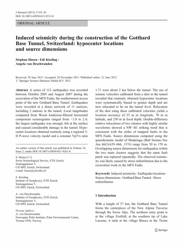
ORIGINAL ARTICLE Induced seismicity during the construction of the Gotthard Base Tunnel, Switzerland: hypocenter locations and source dimensions Stephan Husen & Edi Kissling & Angela von Deschwanden Received: 28 June 2011 / Accepted: 28 November 2011 / Published online: 21 June 2012 # Springer Science+Business Media B.V. 2012 Abstract A series of 112 earthquakes was recorded between October 2005 and August 2007 during the excavation of the MFS Faido, the southernmost access point of the new Gotthard Base Tunnel. Earthquakes were recorded at a dense network of 11 stations, including 2 stations in the tunnel. Local magnitudes computed from Wood–Anderson-filtered horizontal component seismograms ranged from -1.0 to 2.4; the largest earthquake was strongly felt at the surface and caused considerable damage in the tunnel. Hypo- center locations obtained routinely using a regional 3- D P-wave velocity model and a constant Vp/Vs ratio 1.71 were about 2 km below the tunnel. The use of seismic velocities calibrated from a shot in the tunnel revealed that routinely obtained hypocenter locations were systematically biased to greater depth and are now relocated to be on the tunnel level. Relocation of the shot using these calibrated velocities yields a location accuracy of 25 m in longitude, 70 m in latitude, and 250 m in focal depth. Double-difference relative relocations of two clusters with highly similar waveforms showed a NW–SE striking trend that is consistent with the strike of mapped faults in the MFS Faido. Source dimensions computed using the quasidynamic model of Madariaga (Bull Seismo Soc Am 66(3):639–666, 1976) range from 50 to 170 m. Overlapping source dimensions for earthquakes within the two main clusters suggests that the same fault patch was ruptured repeatedly. The observed seismic- ity was likely caused by stress redistribution due to the excavation work in the MFS Faido. Keywords Induced seismicity . Earthquake locations . Source dimensions . Gotthard Base Tunnel . Stress redistribution 1 Introduction With a length of 57 km, the Gotthard Base Tunnel forms the centerpiece of the New Alpine Traverse through the Swiss Alps. The northern entry point is at the village Erstfeld, at the southern tip of Lake Lucerne; it ends at the village Biasca in the Ticino J Seismol (2013) 17:63–81 DOI 10.1007/s10950-012-9313-8 An earlier version of this article was published in Volume 16, Issue 2, under DOI 10.1007/s10950-011-9261-8. S. Husen (*) Swiss Seismological Service, ETH Zurich, Sonneggstrasse 5, CH 8092 Zurich, Switzerland e-mail: [email protected] E. Kissling Institute of Geophysics, ETH Zurich, Sonneggstrasse 5, CH 8092 Zurich, Switzerland A. von Deschwanden Institute of Geophysics, ETH Zurich, Sonneggstrasse 5, CH 8092 Zurich, Switzerland Present Address: A. von Deschwanden Norwegian Polar Institute, Polar Environmental Centre, Tromsø 9296, Norway
Transcript of Induced seismicity during the construction of the Gotthard...
ORIGINAL ARTICLE
Induced seismicity during the construction of the GotthardBase Tunnel, Switzerland: hypocenter locationsand source dimensions
Stephan Husen & Edi Kissling &
Angela von Deschwanden
Received: 28 June 2011 /Accepted: 28 November 2011 /Published online: 21 June 2012# Springer Science+Business Media B.V. 2012
Abstract A series of 112 earthquakes was recordedbetween October 2005 and August 2007 during theexcavation of the MFS Faido, the southernmost accesspoint of the new Gotthard Base Tunnel. Earthquakeswere recorded at a dense network of 11 stations,including 2 stations in the tunnel. Local magnitudescomputed from Wood–Anderson-filtered horizontalcomponent seismograms ranged from −1.0 to 2.4;the largest earthquake was strongly felt at the surfaceand caused considerable damage in the tunnel. Hypo-center locations obtained routinely using a regional 3-D P-wave velocity model and a constant Vp/Vs ratio
1.71 were about 2 km below the tunnel. The use ofseismic velocities calibrated from a shot in the tunnelrevealed that routinely obtained hypocenter locationswere systematically biased to greater depth and arenow relocated to be on the tunnel level. Relocationof the shot using these calibrated velocities yields alocation accuracy of 25 m in longitude, 70 m inlatitude, and 250 m in focal depth. Double-differencerelative relocations of two clusters with highly similarwaveforms showed a NW–SE striking trend that isconsistent with the strike of mapped faults in theMFS Faido. Source dimensions computed using thequasidynamic model of Madariaga (Bull Seismo SocAm 66(3):639–666, 1976) range from 50 to 170 m.Overlapping source dimensions for earthquakes withinthe two main clusters suggests that the same faultpatch was ruptured repeatedly. The observed seismic-ity was likely caused by stress redistribution due to theexcavation work in the MFS Faido.
Keywords Induced seismicity . Earthquake locations .
Source dimensions . Gotthard Base Tunnel . Stressredistribution
1 Introduction
With a length of 57 km, the Gotthard Base Tunnelforms the centerpiece of the New Alpine Traversethrough the Swiss Alps. The northern entry point isat the village Erstfeld, at the southern tip of LakeLucerne; it ends at the village Biasca in the Ticino
J Seismol (2013) 17:63–81DOI 10.1007/s10950-012-9313-8
An earlier version of this article was published in Volume 16,Issue 2, under DOI 10.1007/s10950-011-9261-8.
S. Husen (*)Swiss Seismological Service, ETH Zurich,Sonneggstrasse 5,CH 8092 Zurich, Switzerlande-mail: [email protected]
E. KisslingInstitute of Geophysics, ETH Zurich,Sonneggstrasse 5,CH 8092 Zurich, Switzerland
A. von DeschwandenInstitute of Geophysics, ETH Zurich,Sonneggstrasse 5,CH 8092 Zurich, Switzerland
Present Address:A. von DeschwandenNorwegian Polar Institute, Polar Environmental Centre,Tromsø 9296, Norway
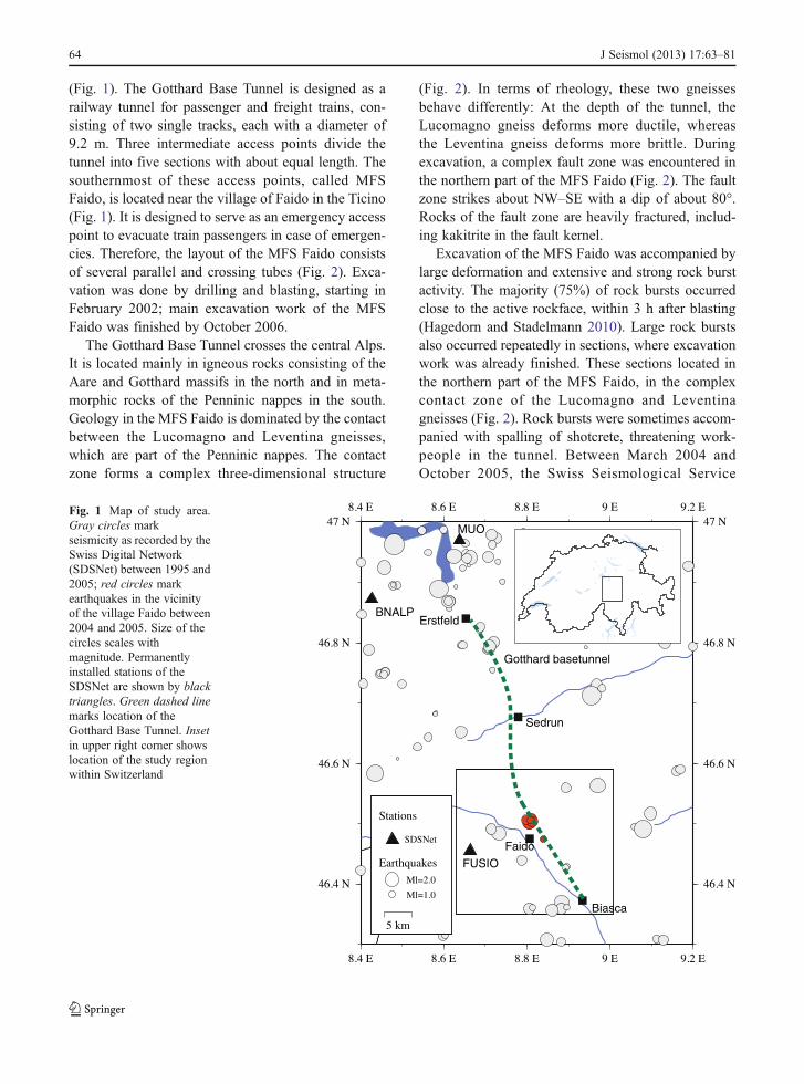
(Fig. 1). The Gotthard Base Tunnel is designed as arailway tunnel for passenger and freight trains, con-sisting of two single tracks, each with a diameter of9.2 m. Three intermediate access points divide thetunnel into five sections with about equal length. Thesouthernmost of these access points, called MFSFaido, is located near the village of Faido in the Ticino(Fig. 1). It is designed to serve as an emergency accesspoint to evacuate train passengers in case of emergen-cies. Therefore, the layout of the MFS Faido consistsof several parallel and crossing tubes (Fig. 2). Exca-vation was done by drilling and blasting, starting inFebruary 2002; main excavation work of the MFSFaido was finished by October 2006.
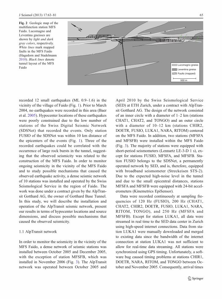
The Gotthard Base Tunnel crosses the central Alps.It is located mainly in igneous rocks consisting of theAare and Gotthard massifs in the north and in meta-morphic rocks of the Penninic nappes in the south.Geology in the MFS Faido is dominated by the contactbetween the Lucomagno and Leventina gneisses,which are part of the Penninic nappes. The contactzone forms a complex three-dimensional structure
(Fig. 2). In terms of rheology, these two gneissesbehave differently: At the depth of the tunnel, theLucomagno gneiss deforms more ductile, whereasthe Leventina gneiss deforms more brittle. Duringexcavation, a complex fault zone was encountered inthe northern part of the MFS Faido (Fig. 2). The faultzone strikes about NW–SE with a dip of about 80°.Rocks of the fault zone are heavily fractured, includ-ing kakitrite in the fault kernel.
Excavation of the MFS Faido was accompanied bylarge deformation and extensive and strong rock burstactivity. The majority (75%) of rock bursts occurredclose to the active rockface, within 3 h after blasting(Hagedorn and Stadelmann 2010). Large rock burstsalso occurred repeatedly in sections, where excavationwork was already finished. These sections located inthe northern part of the MFS Faido, in the complexcontact zone of the Lucomagno and Leventinagneisses (Fig. 2). Rock bursts were sometimes accom-panied with spalling of shotcrete, threatening work-people in the tunnel. Between March 2004 andOctober 2005, the Swiss Seismological Service
Faido
FUSIO
MUO
BNALP
Biasca
Sedrun
Erstfeld
Gotthard basetunnel
5 km
Ml=2.0
SDSNet
Ml=1.0
Earthquakes
Stations
Fig. 1 Map of study area.Gray circles markseismicity as recorded by theSwiss Digital Network(SDSNet) between 1995 and2005; red circles markearthquakes in the vicinityof the village Faido between2004 and 2005. Size of thecircles scales withmagnitude. Permanentlyinstalled stations of theSDSNet are shown by blacktriangles. Green dashed linemarks location of theGotthard Base Tunnel. Insetin upper right corner showslocation of the study regionwithin Switzerland
64 J Seismol (2013) 17:63–81
recorded 12 small earthquakes (ML 0.9–1.6) in thevicinity of the village of Faido (Fig. 1). Prior to March2004, no earthquakes were recorded in this area (Baeret al. 2005). Hypocenter locations of these earthquakeswere poorly constrained due to the low number ofstations of the Swiss Digital Seismic Network(SDSNet) that recorded the events. Only stationFUSIO of the SDSNet was within 10 km distance ofthe epicenters of the events (Fig. 1). Three of therecorded earthquakes could be correlated with theoccurrence of large rock bursts in the tunnel, suggest-ing that the observed seismicity was related to theconstruction of the MFS Faido. In order to monitorongoing seismicity in the vicinity of the MFS Faidoand to study possible mechanisms that caused theobserved earthquake activity, a dense seismic networkof 10 stations was installed and operated by the SwissSeismological Service in the region of Faido. Thework was done under a contract given by the AlpTran-sit Gotthard AG, the owner of Gotthard Base Tunnel.In this study, we will describe the installation andoperation of the AlpTransit seismic network, presentour results in terms of hypocenter locations and sourcedimensions, and discuss possible mechanisms thatcaused the observed seismicity.
1.1 AlpTransit network
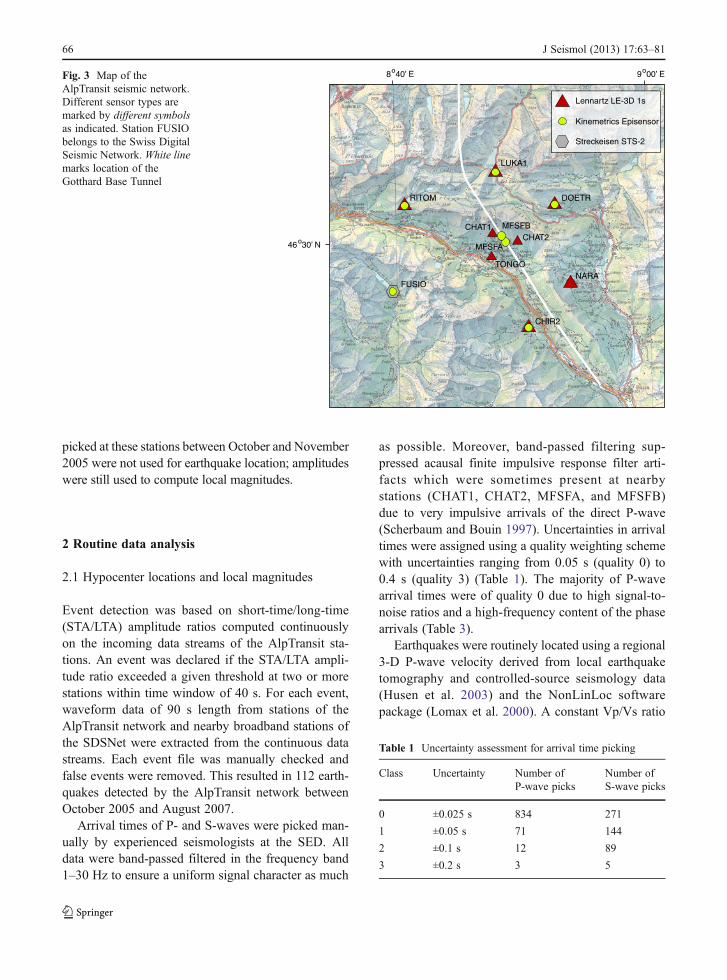
In order to monitor the seismicity in the vicinity of theMFS Faido, a dense network of seismic stations wasinstalled between October 2005 and December 2005,with the exception of station MFSFB, which wasinstalled in November 2006 (Fig. 3). The AlpTransitnetwork was operated between October 2005 and
April 2010 by the Swiss Seismological Service(SED) at ETH Zurich, under a contract with AlpTran-sit Gotthard AG. The design of the network consistedof an inner circle with a diameter of 1–2 km (stationsCHAT1, CHAT2, and TONGO) and an outer circlewith a diameter of 10–12 km (stations CHIR2,DOETR, FUSIO, LUKA1, NARA, RITOM) centeredon the MFS Faido. In addition, two stations (MFSFAand MFSFB) were installed within the MFS Faido(Fig. 3). The majority of stations were equipped withshort-period seismometers (Lennartz LE-3-D 1 s), ex-cept for stations FUSIO, MFSFA, and MFSFB. Sta-tion FUSIO belongs to the SDSNet, a permanentlyoperated network by SED, and is, therefore, equippedwith broadband seismometer (Streckeisen STS-2).Due to the expected high-noise level in the tunneland due to the small epicentral distances, stationsMFSFA and MFSFB were equipped with 24-bit accel-erometers (Kinemetrics EpiSensor).
Data were recorded continuously at sampling fre-quencies of 120 Hz (FUSIO), 200 Hz (CHAT1,CHAT2, CHIR2, DOETR, FUSIO, LUKA1, NARA,RITOM, TONGO), and 250 Hz (MFSFA andMFSFB). Except for station LUKA1, all data werestreamed in real time to the SED data center in Zurichusing high-speed internet connections. Data from sta-tion LUKA1 were manually downloaded and mergedto existing data since the bandwidth of the internetconnection at station LUKA1 was not sufficient toallow for real-time data streaming. All stations weresynchronized using GPS timing. Unfortunately, a soft-ware bug caused timing problems at stations CHIR1,DOETR, NARA, RITOM, and TONGO between Oc-tober and November 2005. Consequently, arrival times
?
?
??
?
?
?
?
?
?
?
?
? ?
?
?
N
705’000
?
706’000??
? ?
?
Lucomagno gneiss
Leventina gneiss
Faults (mapped)
500 m
Fig. 2 Geologic map of themultifunction station MFSFaido. Lucomagno andLeventina gneisses areshown by light and darkgray colors, respectively.White lines mark mappedfaults in the MFS Faido(Hagedorn and Stadelmann2010). Black lines denotetunnel layout of the MFSFaido
J Seismol (2013) 17:63–81 65
picked at these stations between October and November2005 were not used for earthquake location; amplitudeswere still used to compute local magnitudes.
2 Routine data analysis
2.1 Hypocenter locations and local magnitudes
Event detection was based on short-time/long-time(STA/LTA) amplitude ratios computed continuouslyon the incoming data streams of the AlpTransit sta-tions. An event was declared if the STA/LTA ampli-tude ratio exceeded a given threshold at two or morestations within time window of 40 s. For each event,waveform data of 90 s length from stations of theAlpTransit network and nearby broadband stations ofthe SDSNet were extracted from the continuous datastreams. Each event file was manually checked andfalse events were removed. This resulted in 112 earth-quakes detected by the AlpTransit network betweenOctober 2005 and August 2007.
Arrival times of P- and S-waves were picked man-ually by experienced seismologists at the SED. Alldata were band-passed filtered in the frequency band1–30 Hz to ensure a uniform signal character as much
as possible. Moreover, band-passed filtering sup-pressed acausal finite impulsive response filter arti-facts which were sometimes present at nearbystations (CHAT1, CHAT2, MFSFA, and MFSFB)due to very impulsive arrivals of the direct P-wave(Scherbaum and Bouin 1997). Uncertainties in arrivaltimes were assigned using a quality weighting schemewith uncertainties ranging from 0.05 s (quality 0) to0.4 s (quality 3) (Table 1). The majority of P-wavearrival times were of quality 0 due to high signal-to-noise ratios and a high-frequency content of the phasearrivals (Table 3).
Earthquakes were routinely located using a regional3-D P-wave velocity derived from local earthquaketomography and controlled-source seismology data(Husen et al. 2003) and the NonLinLoc softwarepackage (Lomax et al. 2000). A constant Vp/Vs ratio
9 00’ E8 40’ E
46 30’ N
TONGO
MFSFA
MFSFBCHAT1CHAT2
CHIR2
FUSIONARA
LUKA1
DOETRRITOM
Streckeisen STS-2
Lennartz LE-3D 1s
Kinemetrics Episensor
Fig. 3 Map of theAlpTransit seismic network.Different sensor types aremarked by different symbolsas indicated. Station FUSIObelongs to the Swiss DigitalSeismic Network. White linemarks location of theGotthard Base Tunnel
Table 1 Uncertainty assessment for arrival time picking
Class Uncertainty Number ofP-wave picks
Number ofS-wave picks
0 ±0.025 s 834 271
1 ±0.05 s 71 144
2 ±0.1 s 12 89
3 ±0.2 s 3 5
66 J Seismol (2013) 17:63–81
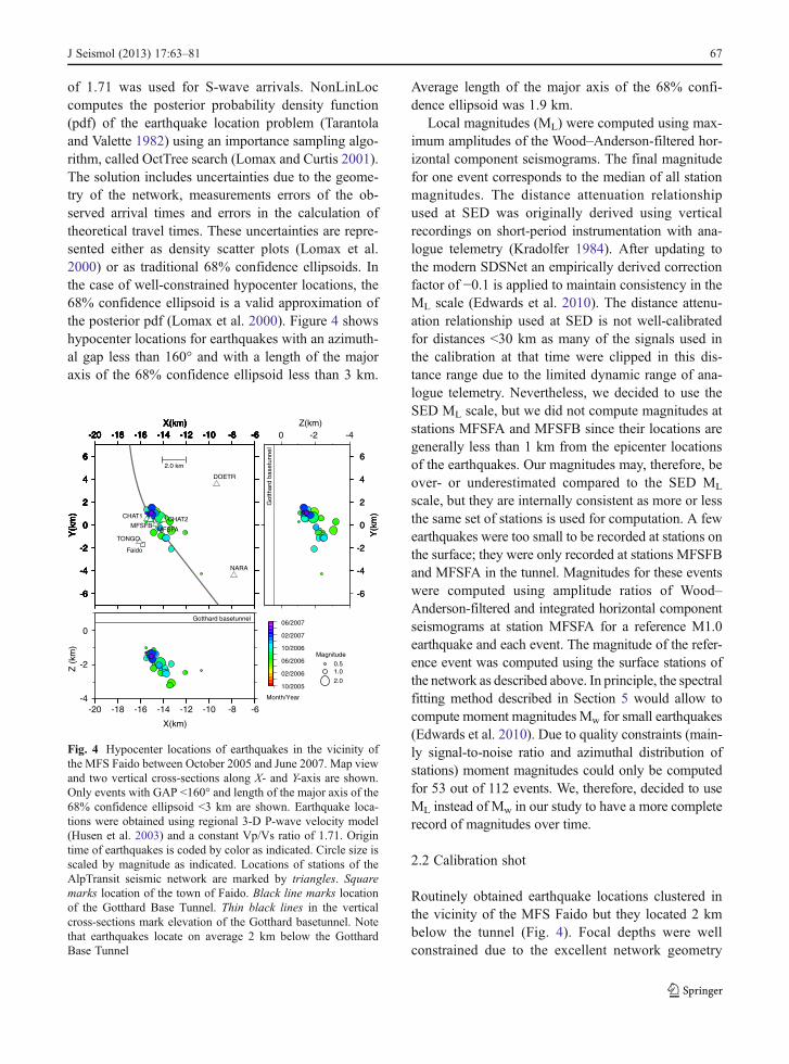
of 1.71 was used for S-wave arrivals. NonLinLoccomputes the posterior probability density function(pdf) of the earthquake location problem (Tarantolaand Valette 1982) using an importance sampling algo-rithm, called OctTree search (Lomax and Curtis 2001).The solution includes uncertainties due to the geome-try of the network, measurements errors of the ob-served arrival times and errors in the calculation oftheoretical travel times. These uncertainties are repre-sented either as density scatter plots (Lomax et al.2000) or as traditional 68% confidence ellipsoids. Inthe case of well-constrained hypocenter locations, the68% confidence ellipsoid is a valid approximation ofthe posterior pdf (Lomax et al. 2000). Figure 4 showshypocenter locations for earthquakes with an azimuth-al gap less than 160° and with a length of the majoraxis of the 68% confidence ellipsoid less than 3 km.
Average length of the major axis of the 68% confi-dence ellipsoid was 1.9 km.
Local magnitudes (ML) were computed using max-imum amplitudes of the Wood–Anderson-filtered hor-izontal component seismograms. The final magnitudefor one event corresponds to the median of all stationmagnitudes. The distance attenuation relationshipused at SED was originally derived using verticalrecordings on short-period instrumentation with ana-logue telemetry (Kradolfer 1984). After updating tothe modern SDSNet an empirically derived correctionfactor of −0.1 is applied to maintain consistency in theML scale (Edwards et al. 2010). The distance attenu-ation relationship used at SED is not well-calibratedfor distances <30 km as many of the signals used inthe calibration at that time were clipped in this dis-tance range due to the limited dynamic range of ana-logue telemetry. Nevertheless, we decided to use theSED ML scale, but we did not compute magnitudes atstations MFSFA and MFSFB since their locations aregenerally less than 1 km from the epicenter locationsof the earthquakes. Our magnitudes may, therefore, beover- or underestimated compared to the SED ML
scale, but they are internally consistent as more or lessthe same set of stations is used for computation. A fewearthquakes were too small to be recorded at stations onthe surface; they were only recorded at stations MFSFBand MFSFA in the tunnel. Magnitudes for these eventswere computed using amplitude ratios of Wood–Anderson-filtered and integrated horizontal componentseismograms at station MFSFA for a reference M1.0earthquake and each event. The magnitude of the refer-ence event was computed using the surface stations ofthe network as described above. In principle, the spectralfitting method described in Section 5 would allow tocompute moment magnitudes Mw for small earthquakes(Edwards et al. 2010). Due to quality constraints (main-ly signal-to-noise ratio and azimuthal distribution ofstations) moment magnitudes could only be computedfor 53 out of 112 events. We, therefore, decided to useML instead of Mw in our study to have a more completerecord of magnitudes over time.
2.2 Calibration shot
Routinely obtained earthquake locations clustered inthe vicinity of the MFS Faido but they located 2 kmbelow the tunnel (Fig. 4). Focal depths were wellconstrained due to the excellent network geometry
-20 -18 -16 -14 -12 -10 -8 -6X(km)
-20 -18 -16 -14 -12 -10 -8 -6X(km)
-20 -18 -16 -14 -12 -10 -8 -6X(km)
-20 -18 -16 -14 -12 -10 -8 -6X(km)
-20 -18 -16 -14 -12 -10 -8 -6X(km)
-20 -18 -16 -14 -12 -10 -8 -6X(km)
-20 -18 -16 -14 -12 -10 -8 -6X(km) Z(km)
-20 -18 -16 -14 -12 -10 -8 -6
X(km)
-6
-4
-2
0
2
4
6
Y(k
m)
-6
-4
-2
0
2
4
6
Y(k
m)
-6
-4
-2
0
2
4
6
Y(k
m)
-6
-4
-2
0
2
4
6
Y(k
m)
-6
-4
-2
0
2
4
6
Y(k
m)
-6
-4
-2
0
2
4
6
Y(k
m)
-6
-4
-2
0
-4
-2
0
2
4
6
Y(k
m)
Z (
km)
-6
-4
-2
0
2
4
6
Y(k
m)
-6
-4
-4
-2
-2
0
0
2
4
6
Y(k
m)
Gotthard basetunnel
Got
thar
d ba
setu
nnel
10/2005
Month/Year
02/2006
06/2006
10/2006
02/2007
06/2007
0.51.0
2.0
Magnitude
2.0 km
Faido
MFSFAMFSFB
CHAT1 CHAT2
TONGO
NARA
DOETR
Fig. 4 Hypocenter locations of earthquakes in the vicinity ofthe MFS Faido between October 2005 and June 2007. Map viewand two vertical cross-sections along X- and Y-axis are shown.Only events with GAP <160° and length of the major axis of the68% confidence ellipsoid <3 km are shown. Earthquake loca-tions were obtained using regional 3-D P-wave velocity model(Husen et al. 2003) and a constant Vp/Vs ratio of 1.71. Origintime of earthquakes is coded by color as indicated. Circle size isscaled by magnitude as indicated. Locations of stations of theAlpTransit seismic network are marked by triangles. Squaremarks location of the town of Faido. Black line marks locationof the Gotthard Base Tunnel. Thin black lines in the verticalcross-sections mark elevation of the Gotthard basetunnel. Notethat earthquakes locate on average 2 km below the GotthardBase Tunnel
J Seismol (2013) 17:63–81 67
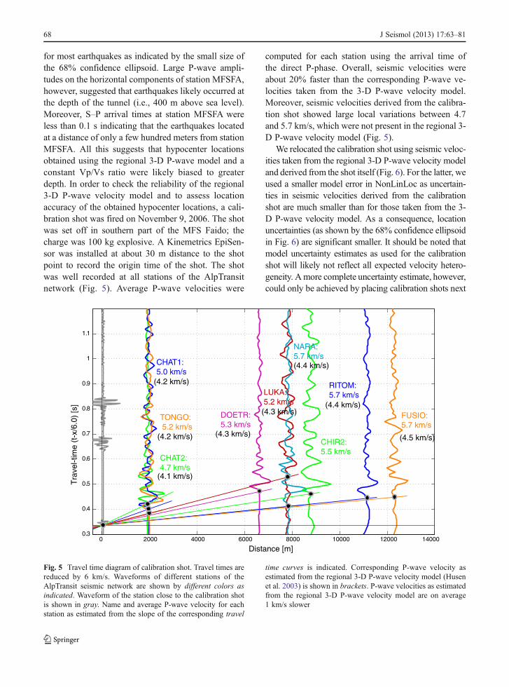
for most earthquakes as indicated by the small size ofthe 68% confidence ellipsoid. Large P-wave ampli-tudes on the horizontal components of station MFSFA,however, suggested that earthquakes likely occurred atthe depth of the tunnel (i.e., 400 m above sea level).Moreover, S–P arrival times at station MFSFA wereless than 0.1 s indicating that the earthquakes locatedat a distance of only a few hundred meters from stationMFSFA. All this suggests that hypocenter locationsobtained using the regional 3-D P-wave model and aconstant Vp/Vs ratio were likely biased to greaterdepth. In order to check the reliability of the regional3-D P-wave velocity model and to assess locationaccuracy of the obtained hypocenter locations, a cali-bration shot was fired on November 9, 2006. The shotwas set off in southern part of the MFS Faido; thecharge was 100 kg explosive. A Kinemetrics EpiSen-sor was installed at about 30 m distance to the shotpoint to record the origin time of the shot. The shotwas well recorded at all stations of the AlpTransitnetwork (Fig. 5). Average P-wave velocities were
computed for each station using the arrival time ofthe direct P-phase. Overall, seismic velocities wereabout 20% faster than the corresponding P-wave ve-locities taken from the 3-D P-wave velocity model.Moreover, seismic velocities derived from the calibra-tion shot showed large local variations between 4.7and 5.7 km/s, which were not present in the regional 3-D P-wave velocity model (Fig. 5).
We relocated the calibration shot using seismic veloc-ities taken from the regional 3-D P-wave velocity modeland derived from the shot itself (Fig. 6). For the latter, weused a smaller model error in NonLinLoc as uncertain-ties in seismic velocities derived from the calibrationshot are much smaller than for those taken from the 3-D P-wave velocity model. As a consequence, locationuncertainties (as shown by the 68% confidence ellipsoidin Fig. 6) are significant smaller. It should be noted thatmodel uncertainty estimates as used for the calibrationshot will likely not reflect all expected velocity hetero-geneity. Amore complete uncertainty estimate, however,could only be achieved by placing calibration shots next
0 2000 4000 6000 8000 10000 12000 140000.3
0.4
0.5
0.6
0.7
0.8
0.9
1
1.1
Distance [m]
Tra
vel-t
ime
(t-x
/6.0
) [s
]
CHAT2: 4.7 km/s
CHAT1: 5.0 km/s
(4.2 km/s)
(4.2 km/s) (4.3 km/s)
(4.3 km/s)
(4.5 km/s)
(4.4 km/s)
(4.4 km/s)
(4.1 km/s)
TONGO: 5.2 km/s
DOETR: 5.3 km/s
LUKA: 5.2 km/s
NARA: 5.7 km/s
CHIR2: 5.5 km/s
RITOM: 5.7 km/s
FUSIO: 5.7 km/s
Fig. 5 Travel time diagram of calibration shot. Travel times arereduced by 6 km/s. Waveforms of different stations of theAlpTransit seismic network are shown by different colors asindicated. Waveform of the station close to the calibration shotis shown in gray. Name and average P-wave velocity for eachstation as estimated from the slope of the corresponding travel
time curves is indicated. Corresponding P-wave velocity asestimated from the regional 3-D P-wave velocity model (Husenet al. 2003) is shown in brackets. P-wave velocities as estimatedfrom the regional 3-D P-wave velocity model are on average1 km/s slower
68 J Seismol (2013) 17:63–81
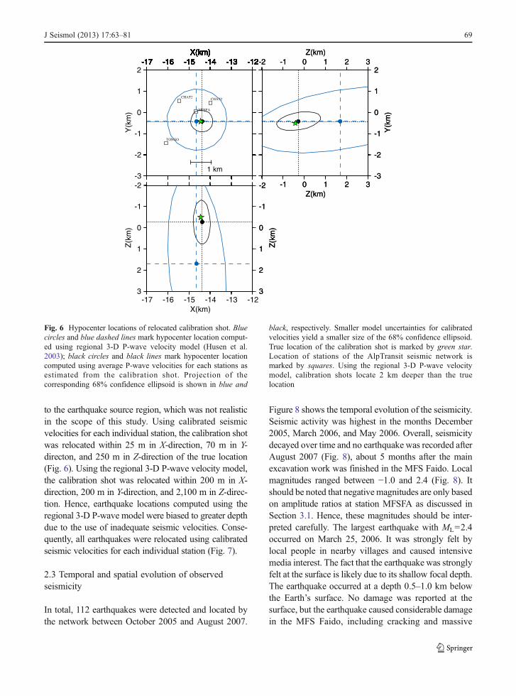
to the earthquake source region, which was not realisticin the scope of this study. Using calibrated seismicvelocities for each individual station, the calibration shotwas relocated within 25 m in X-direction, 70 m in Y-directon, and 250 m in Z-direction of the true location(Fig. 6). Using the regional 3-D P-wave velocity model,the calibration shot was relocated within 200 m in X-direction, 200 m in Y-direction, and 2,100 m in Z-direc-tion. Hence, earthquake locations computed using theregional 3-D P-wave model were biased to greater depthdue to the use of inadequate seismic velocities. Conse-quently, all earthquakes were relocated using calibratedseismic velocities for each individual station (Fig. 7).
2.3 Temporal and spatial evolution of observedseismicity
In total, 112 earthquakes were detected and located bythe network between October 2005 and August 2007.
Figure 8 shows the temporal evolution of the seismicity.Seismic activity was highest in the months December2005, March 2006, and May 2006. Overall, seismicitydecayed over time and no earthquake was recorded afterAugust 2007 (Fig. 8), about 5 months after the mainexcavation work was finished in the MFS Faido. Localmagnitudes ranged between −1.0 and 2.4 (Fig. 8). Itshould be noted that negative magnitudes are only basedon amplitude ratios at station MFSFA as discussed inSection 3.1. Hence, these magnitudes should be inter-preted carefully. The largest earthquake with ML02.4occurred on March 25, 2006. It was strongly felt bylocal people in nearby villages and caused intensivemedia interest. The fact that the earthquake was stronglyfelt at the surface is likely due to its shallow focal depth.The earthquake occurred at a depth 0.5–1.0 km belowthe Earth’s surface. No damage was reported at thesurface, but the earthquake caused considerable damagein the MFS Faido, including cracking and massive
Z(k
m)
-2
-1
0
1
2
3
Z(k
m)
-2
-1
0
1
2
3
-2
-1
0
1
2
3
Z(k
m)
-17 -16 -15 -14 -13 -12X(km)
0
Y(k
m)
-17 -16 -15 -14 -13 -12X(km)
MFSFA
-17 -16 -15 -14 -13 -12X(km)
CHAT2
-17 -16 -15 -14 -13 -12X(km)
-17 -16 -15 -14 -13 -12X(km)
CHAT2
-17 -16 -15 -14 -13 -12X(km)
TONGO
-17 -16 -15 -14 -13 -12X(km)
-17 -16 -15 -14 -13 -12X(km)
-17 -16 -15 -14 -13 -12X(km)
-17 -16 -15 -14 -13 -12X(km)
-17 -16 -15 -14 -13 -12X(km)
-17 -16 -15 -14 -13 -12X(km)
-17 -16 -15 -14 -13 -12X(km)
-17 -16 -15 -14 -13 -12X(km)
-3
-2
-1
1
2-17 -16 -15 -14 -13 -12
X(km)
1 km-3
-2
-1
0
1
2
Y(k
m)
-1 0 1 2 3Z(km)
-2 -1 0 1 2 3Z(km)
-3
-2
-1
0
1
2
Y(k
m)
-1 0 1 2 3Z(km)
-2 -1 0 1 2 3Z(km)
Fig. 6 Hypocenter locations of relocated calibration shot. Bluecircles and blue dashed lines mark hypocenter location comput-ed using regional 3-D P-wave velocity model (Husen et al.2003); black circles and black lines mark hypocenter locationcomputed using average P-wave velocities for each stations asestimated from the calibration shot. Projection of thecorresponding 68% confidence ellipsoid is shown in blue and
black, respectively. Smaller model uncertainties for calibratedvelocities yield a smaller size of the 68% confidence ellipsoid.True location of the calibration shot is marked by green star.Location of stations of the AlpTransit seismic network ismarked by squares. Using the regional 3-D P-wave velocitymodel, calibration shots locate 2 km deeper than the truelocation
J Seismol (2013) 17:63–81 69
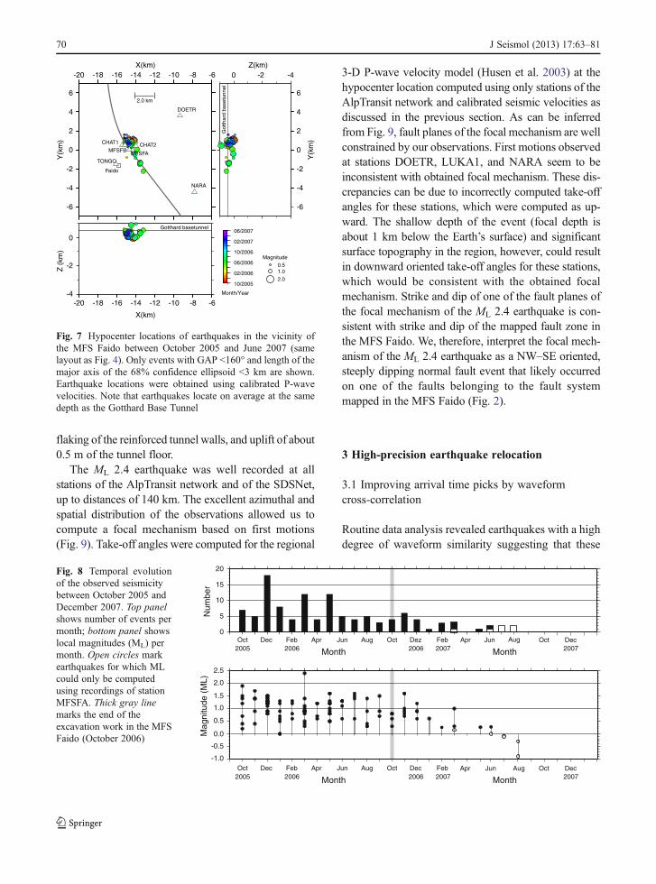
flaking of the reinforced tunnel walls, and uplift of about0.5 m of the tunnel floor.
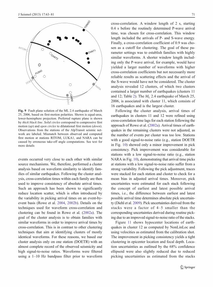
The ML 2.4 earthquake was well recorded at allstations of the AlpTransit network and of the SDSNet,up to distances of 140 km. The excellent azimuthal andspatial distribution of the observations allowed us tocompute a focal mechanism based on first motions(Fig. 9). Take-off angles were computed for the regional
3-D P-wave velocity model (Husen et al. 2003) at thehypocenter location computed using only stations of theAlpTransit network and calibrated seismic velocities asdiscussed in the previous section. As can be inferredfrom Fig. 9, fault planes of the focal mechanism are wellconstrained by our observations. First motions observedat stations DOETR, LUKA1, and NARA seem to beinconsistent with obtained focal mechanism. These dis-crepancies can be due to incorrectly computed take-offangles for these stations, which were computed as up-ward. The shallow depth of the event (focal depth isabout 1 km below the Earth’s surface) and significantsurface topography in the region, however, could resultin downward oriented take-off angles for these stations,which would be consistent with the obtained focalmechanism. Strike and dip of one of the fault planes ofthe focal mechanism of the ML 2.4 earthquake is con-sistent with strike and dip of the mapped fault zone inthe MFS Faido. We, therefore, interpret the focal mech-anism of the ML 2.4 earthquake as a NW–SE oriented,steeply dipping normal fault event that likely occurredon one of the faults belonging to the fault systemmapped in the MFS Faido (Fig. 2).
3 High-precision earthquake relocation
3.1 Improving arrival time picks by waveformcross-correlation
Routine data analysis revealed earthquakes with a highdegree of waveform similarity suggesting that these
-20 -18 -16 -14 -12 -10 -8 -6X(km) Z(km)
-20 -18 -16 -14 -12 -10 -8 -6
X(km)
-6
-4
-2
0
-4
-2
0
2
4
6
Y(k
m)
Z (
km)
-6
-4
-4
-2
-2
0
0
2
4
6
Y(k
m)
Gotthard basetunnelG
otth
ard
base
tunn
el
10/2005
Month/Year
02/2006
06/2006
10/2006
02/2007
06/2007
0.51.0
2.0
Magnitude
2.0 km
Faido
MFSFAMFSFB
CHAT1 CHAT2
TONGO
NARA
DOETR
Fig. 7 Hypocenter locations of earthquakes in the vicinity ofthe MFS Faido between October 2005 and June 2007 (samelayout as Fig. 4). Only events with GAP <160° and length of themajor axis of the 68% confidence ellipsoid <3 km are shown.Earthquake locations were obtained using calibrated P-wavevelocities. Note that earthquakes locate on average at the samedepth as the Gotthard Base Tunnel
0.5
0.0
-0.5
-1.0
1.0
1.5
2.0
2.5
Mag
nitu
de (
ML)
Oct Dec Feb Apr Jun Aug Oct FebDec
Month MonthApr Jun Aug Oct Dec
2005 2006 2006 2007 2007
Oct2005 2006 2006 2007 2007
Dec Feb Apr Jun Aug Oct Feb Apr Jun AugDez
Month Month
0
5
10
15
20
Num
ber
Oct Dec
Fig. 8 Temporal evolutionof the observed seismicitybetween October 2005 andDecember 2007. Top panelshows number of events permonth; bottom panel showslocal magnitudes (ML) permonth. Open circles markearthquakes for which MLcould only be computedusing recordings of stationMFSFA. Thick gray linemarks the end of theexcavation work in the MFSFaido (October 2006)
70 J Seismol (2013) 17:63–81
events occurred very close to each other with similarsource mechanisms. We, therefore, performed a clusteranalysis based on waveform similarity to identify fam-ilies of similar earthquakes. Following the cluster anal-ysis, cross-correlation times within each family are thenused to improve consistency of absolute arrival times.Such an approach has been shown to significantlyreduce location scatter, which is often introduced bythe variability in picking arrival times on an event-by-event basis (Rowe et al. 2004, 2002b). Details on thetechniques used for waveform cross-correlation andclustering can be found in Rowe et al. (2002a). Thegoal of the cluster analysis is to obtain families withsimilar waveforms in order to improve arrival times bycross-correlation. This is in contrast to other clusteringtechniques that aim at identifying clusters of mostlyidentical waveforms. For these reasons, we based ourcluster analysis only on one station (DOETR) with analmost complete record of the observed seismicity andhigh signal-to-noise ratios. Waveforms were filteredusing a 1–10 Hz bandpass filter prior to waveform
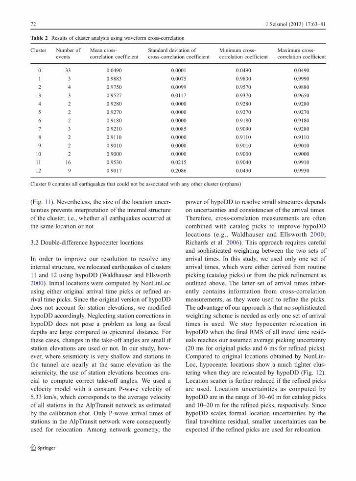
cross-correlation. A window length of 2 s, starting0.4 s before the routinely determined P-wave arrivaltime, was chosen for cross-correlation. This windowlength included the arrivals of P- and S-wave energy.Finally, a cross-correlation coefficient of 0.9 was cho-sen as a cutoff for clustering. The goal of these pa-rameter settings was to establish families with highlysimilar waveforms. A shorter window length includ-ing only the P-wave arrival, for example, would haveyielded a larger number of waveforms with highercross-correlation coefficients but not necessarily morereliable results as scattering effects and the arrival ofthe S-wave would have not be considered. The clusteranalysis revealed 12 clusters, of which two clusterscontained a larger number of earthquakes (clusters 11and 12; Table 2). TheML 2.4 earthquake of March 25,2006, is associated with cluster 11, which consists of16 earthquakes and is the largest cluster.
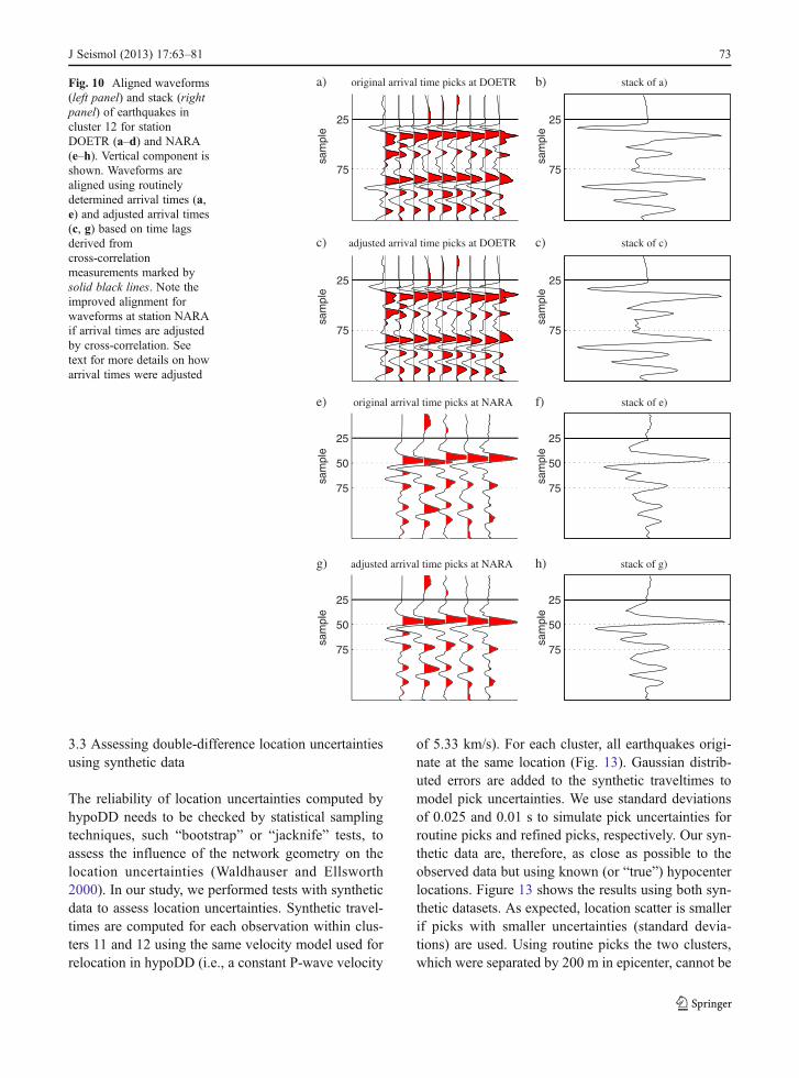
Following the cluster analysis, arrival times ofearthquakes in clusters 11 and 12 were refined usingcross-correlation time lags for each station following theapproach of Rowe et al. (2002a). Arrival times of earth-quakes in the remaining clusters were not adjusted, asthe number of events per cluster was too low. Stationswith a good signal-to-noise ratio (e.g., station DOETRin Fig. 10) showed only a minor improvement in pickconsistency. Pick improvement was considerable forstations with a low signal-to-noise ratio (e.g., stationNARA in Fig. 10), demonstrating that arrival time picksat stations with a low signal-to-noise ratio suffer from astrong variability. Following the pick adjustment, traceswere stacked for each station and cluster to check for amean bias in adjusted arrival times. Moreover, pickuncertainties were estimated for each stack followingthe concept of earliest and latest possible arrivaltimes, i.e., the difference between earliest and latestpossible arrival time determines absolute pick uncertain-ty (Diehl et al. 2009). Pick uncertainties derived from thestacks were a factor of 4–5 smaller than thecorresponding uncertainties derived during routine pick-ing due to an improved signal-to-noise ratio of the stacks.
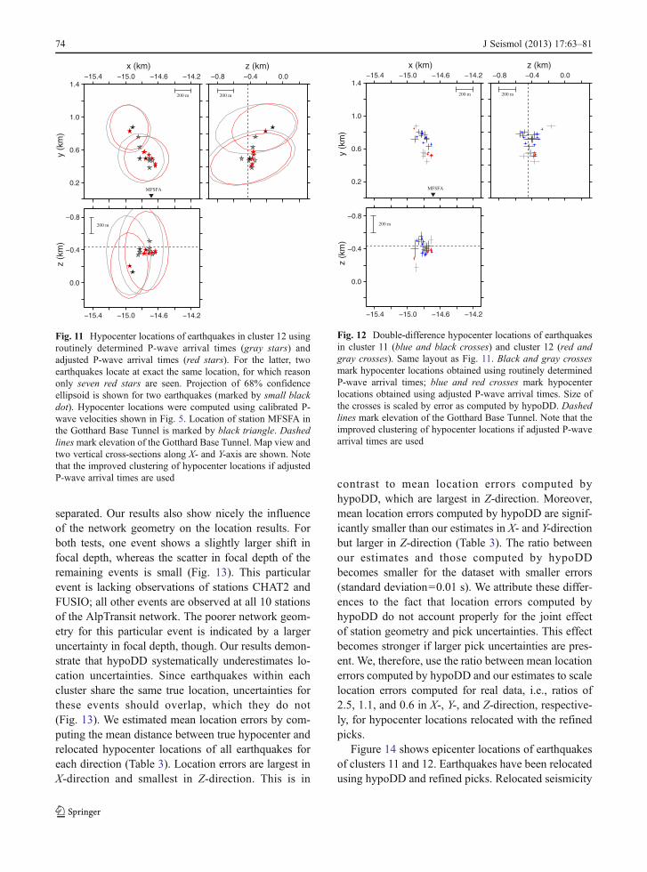
Figure 11 shows hypocenter locations of earth-quakes in cluster 12 as computed by NonLinLoc andusing velocities as estimated from the calibration shot.The improvement in picking consistency yields a tightclustering in epicenter location and focal depth. Loca-tion uncertainties as outlined by the 68% confidenceellipsoid were also slightly reduced due to reducedpicking uncertainties as estimated from the stacks
CHAT2
CHAT1
TON
GO
DOETR
LUK
A1
NARA
CH
IR2
RITOM
FUSIO
Fig. 9 Fault plane solution of the ML 2.4 earthquake of March25, 2006, based on first-motion polarities. Shown is equal-area,lower-hemisphere projection. Preferred rupture plane is shownby thick black line. Solid circles correspond to compressive firstmotion (up) and open circles to dilatational first motion (down).Observations from the stations of the AlpTransit seismic net-work are labeled. Mismatch between observed and computedfirst motion at stations RITOM, LUKA1, and NARA can becaused by erroneous take-off angle computations. See text formore details
J Seismol (2013) 17:63–81 71
(Fig. 11). Nevertheless, the size of the location uncer-tainties prevents interpretation of the internal structureof the cluster, i.e., whether all earthquakes occurred atthe same location or not.
3.2 Double-difference hypocenter locations
In order to improve our resolution to resolve anyinternal structure, we relocated earthquakes of clusters11 and 12 using hypoDD (Waldhauser and Ellsworth2000). Initial locations were computed by NonLinLocusing either original arrival time picks or refined ar-rival time picks. Since the original version of hypoDDdoes not account for station elevations, we modifiedhypoDD accordingly. Neglecting station corrections inhypoDD does not pose a problem as long as focaldepths are large compared to epicentral distance. Forthese cases, changes in the take-off angles are small ifstation elevations are used or not. In our study, how-ever, where seismicity is very shallow and stations inthe tunnel are nearly at the same elevation as theseismicity, the use of station elevations becomes cru-cial to compute correct take-off angles. We used avelocity model with a constant P-wave velocity of5.33 km/s, which corresponds to the average velocityof all stations in the AlpTransit network as estimatedby the calibration shot. Only P-wave arrival times ofstations in the AlpTransit network were consequentlyused for relocation. Among network geometry, the
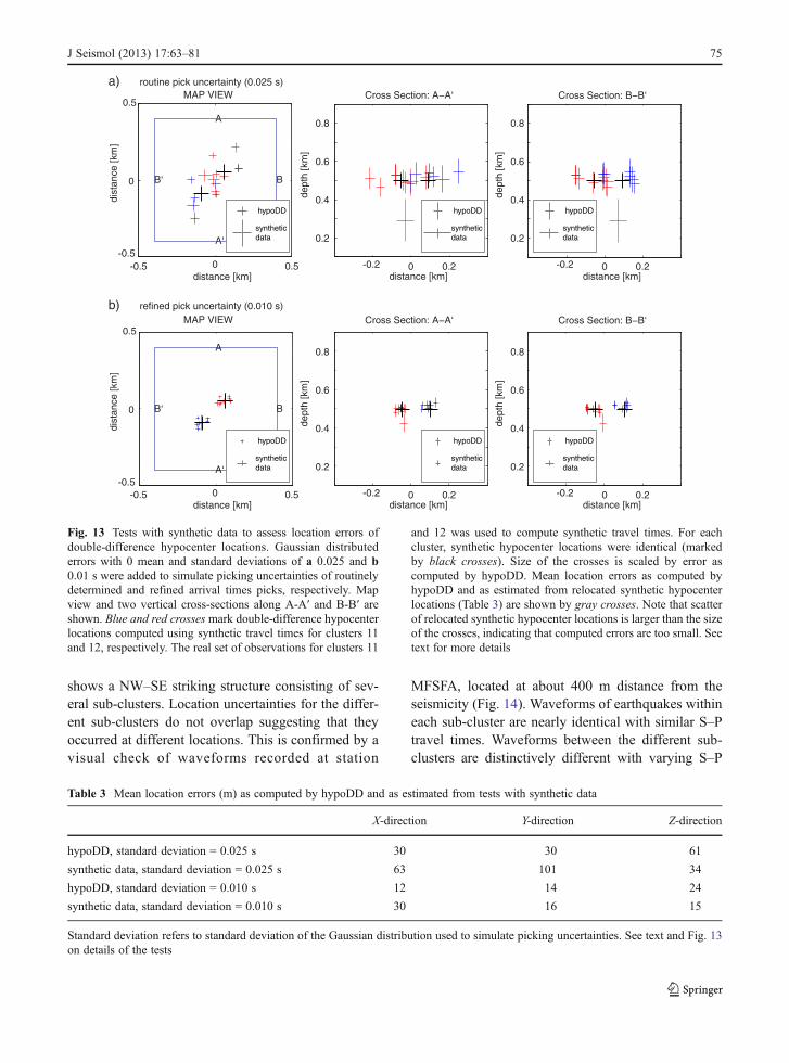
power of hypoDD to resolve small structures dependson uncertainties and consistencies of the arrival times.Therefore, cross-correlation measurements are oftencombined with catalog picks to improve hypoDDlocations (e.g., Waldhauser and Ellsworth 2000;Richards et al. 2006). This approach requires carefuland sophisticated weighting between the two sets ofarrival times. In this study, we used only one set ofarrival times, which were either derived from routinepicking (catalog picks) or from the pick refinement asoutlined above. The latter set of arrival times inher-ently contains information from cross-correlationmeasurements, as they were used to refine the picks.The advantage of our approach is that no sophisticatedweighting scheme is needed as only one set of arrivaltimes is used. We stop hypocenter relocation inhypoDD when the final RMS of all travel time resid-uals reaches our assumed average picking uncertainty(20 ms for original picks and 6 ms for refined picks).Compared to original locations obtained by NonLin-Loc, hypocenter locations show a much tighter clus-tering when they are relocated by hypoDD (Fig. 12).Location scatter is further reduced if the refined picksare used. Location uncertainties as computed byhypoDD are in the range of 30–60 m for catalog picksand 10–20 m for the refined picks, respectively. SincehypoDD scales formal location uncertainties by thefinal traveltime residual, smaller uncertainties can beexpected if the refined picks are used for relocation.
Table 2 Results of cluster analysis using waveform cross-correlation
Cluster Number ofevents
Mean cross-correlation coefficient
Standard deviation ofcross-correlation coefficient
Minimum cross-correlation coefficient
Maximum cross-correlation coefficient
0 33 0.0490 0.0001 0.0490 0.0490
1 3 0.9883 0.0075 0.9830 0.9990
2 4 0.9750 0.0099 0.9570 0.9880
3 3 0.9527 0.0117 0.9370 0.9650
4 2 0.9280 0.0000 0.9280 0.9280
5 2 0.9270 0.0000 0.9270 0.9270
6 2 0.9180 0.0000 0.9180 0.9180
7 3 0.9210 0.0085 0.9090 0.9280
8 2 0.9110 0.0000 0.9110 0.9110
9 2 0.9010 0.0000 0.9010 0.9010
10 2 0.9000 0.0000 0.9000 0.9000
11 16 0.9530 0.0215 0.9040 0.9910
12 9 0.9017 0.2086 0.0490 0.9930
Cluster 0 contains all earthquakes that could not be associated with any other cluster (orphans)
72 J Seismol (2013) 17:63–81
3.3 Assessing double-difference location uncertaintiesusing synthetic data
The reliability of location uncertainties computed byhypoDD needs to be checked by statistical samplingtechniques, such “bootstrap” or “jacknife” tests, toassess the influence of the network geometry on thelocation uncertainties (Waldhauser and Ellsworth2000). In our study, we performed tests with syntheticdata to assess location uncertainties. Synthetic travel-times are computed for each observation within clus-ters 11 and 12 using the same velocity model used forrelocation in hypoDD (i.e., a constant P-wave velocity
of 5.33 km/s). For each cluster, all earthquakes origi-nate at the same location (Fig. 13). Gaussian distrib-uted errors are added to the synthetic traveltimes tomodel pick uncertainties. We use standard deviationsof 0.025 and 0.01 s to simulate pick uncertainties forroutine picks and refined picks, respectively. Our syn-thetic data are, therefore, as close as possible to theobserved data but using known (or “true”) hypocenterlocations. Figure 13 shows the results using both syn-thetic datasets. As expected, location scatter is smallerif picks with smaller uncertainties (standard devia-tions) are used. Using routine picks the two clusters,which were separated by 200 m in epicenter, cannot be
25
75
original arrival time picks at DOETRa) b)
c)
f)
h)
c)
e)
g)
sam
ple
sam
ple
sam
ple
sam
ple
stack of a)
adjusted arrival time picks at DOETR stack of c)
25
75
25
75
25
75
25
50
75
25
50
75
25
50
75
25
50
75
original arrival time picks at NARA
sam
ple
sam
ple
sam
ple
sam
ple
stack of e)
adjusted arrival time picks at NARA stack of g)
Fig. 10 Aligned waveforms(left panel) and stack (rightpanel) of earthquakes incluster 12 for stationDOETR (a–d) and NARA(e–h). Vertical component isshown. Waveforms arealigned using routinelydetermined arrival times (a,e) and adjusted arrival times(c, g) based on time lagsderived fromcross-correlationmeasurements marked bysolid black lines. Note theimproved alignment forwaveforms at station NARAif arrival times are adjustedby cross-correlation. Seetext for more details on howarrival times were adjusted
J Seismol (2013) 17:63–81 73
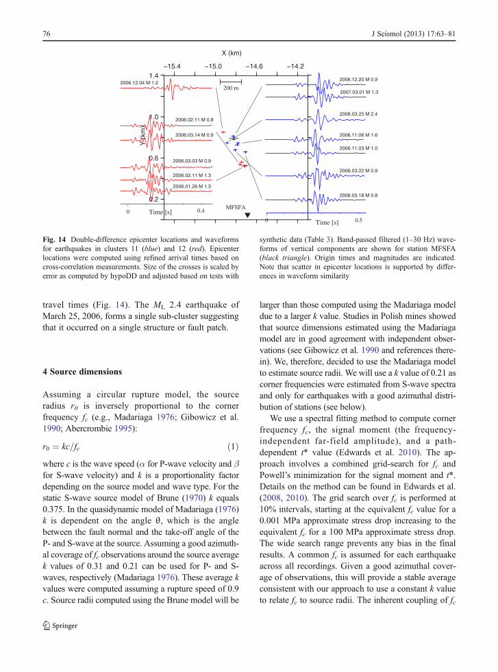
separated. Our results also show nicely the influenceof the network geometry on the location results. Forboth tests, one event shows a slightly larger shift infocal depth, whereas the scatter in focal depth of theremaining events is small (Fig. 13). This particularevent is lacking observations of stations CHAT2 andFUSIO; all other events are observed at all 10 stationsof the AlpTransit network. The poorer network geom-etry for this particular event is indicated by a largeruncertainty in focal depth, though. Our results demon-strate that hypoDD systematically underestimates lo-cation uncertainties. Since earthquakes within eachcluster share the same true location, uncertainties forthese events should overlap, which they do not(Fig. 13). We estimated mean location errors by com-puting the mean distance between true hypocenter andrelocated hypocenter locations of all earthquakes foreach direction (Table 3). Location errors are largest inX-direction and smallest in Z-direction. This is in
contrast to mean location errors computed byhypoDD, which are largest in Z-direction. Moreover,mean location errors computed by hypoDD are signif-icantly smaller than our estimates in X- and Y-directionbut larger in Z-direction (Table 3). The ratio betweenour estimates and those computed by hypoDDbecomes smaller for the dataset with smaller errors(standard deviation00.01 s). We attribute these differ-ences to the fact that location errors computed byhypoDD do not account properly for the joint effectof station geometry and pick uncertainties. This effectbecomes stronger if larger pick uncertainties are pres-ent. We, therefore, use the ratio between mean locationerrors computed by hypoDD and our estimates to scalelocation errors computed for real data, i.e., ratios of2.5, 1.1, and 0.6 in X-, Y-, and Z-direction, respective-ly, for hypocenter locations relocated with the refinedpicks.
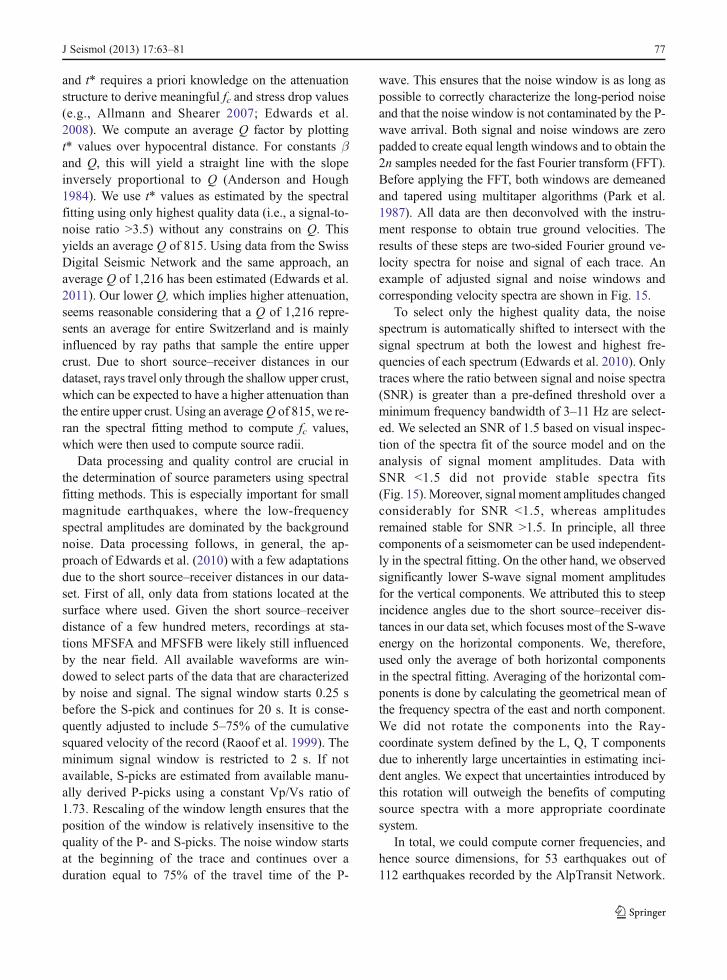
Figure 14 shows epicenter locations of earthquakesof clusters 11 and 12. Earthquakes have been relocatedusing hypoDD and refined picks. Relocated seismicity
−0.8
−0.4
0.0
−15.4 −15.0 −14.6 −14.2
0.2
0.6
1.0
1.4
y (k
m)
z (k
m)
−15.4 −15.0 −14.6 −14.2x (km) z (km)
−0.8 −0.4 0.0
MFSFA
200 m 200 m
200 m
Fig. 11 Hypocenter locations of earthquakes in cluster 12 usingroutinely determined P-wave arrival times (gray stars) andadjusted P-wave arrival times (red stars). For the latter, twoearthquakes locate at exact the same location, for which reasononly seven red stars are seen. Projection of 68% confidenceellipsoid is shown for two earthquakes (marked by small blackdot). Hypocenter locations were computed using calibrated P-wave velocities shown in Fig. 5. Location of station MFSFA inthe Gotthard Base Tunnel is marked by black triangle. Dashedlinesmark elevation of the Gotthard Base Tunnel. Map view andtwo vertical cross-sections along X- and Y-axis are shown. Notethat the improved clustering of hypocenter locations if adjustedP-wave arrival times are used
−0.8
−0.4
0.0
−15.4 −15.0 −14.6 −14.2
0.2
0.6
1.0
1.4
y (k
m)
z (k
m)
−15.4 −15.0 −14.6 −14.2x (km) z (km)
−0.8 −0.4 0.0
MFSFA
200 m 200 m
200 m
Fig. 12 Double-difference hypocenter locations of earthquakesin cluster 11 (blue and black crosses) and cluster 12 (red andgray crosses). Same layout as Fig. 11. Black and gray crossesmark hypocenter locations obtained using routinely determinedP-wave arrival times; blue and red crosses mark hypocenterlocations obtained using adjusted P-wave arrival times. Size ofthe crosses is scaled by error as computed by hypoDD. Dashedlines mark elevation of the Gotthard Base Tunnel. Note that theimproved clustering of hypocenter locations if adjusted P-wavearrival times are used
74 J Seismol (2013) 17:63–81
shows a NW–SE striking structure consisting of sev-eral sub-clusters. Location uncertainties for the differ-ent sub-clusters do not overlap suggesting that theyoccurred at different locations. This is confirmed by avisual check of waveforms recorded at station
MFSFA, located at about 400 m distance from theseismicity (Fig. 14). Waveforms of earthquakes withineach sub-cluster are nearly identical with similar S–Ptravel times. Waveforms between the different sub-clusters are distinctively different with varying S–P
MAP VIEWroutine pick uncertainty (0.025 s)a)
b)
distance [km]
0.5
0.8
0.6
0.4
0.2
-0.2 0.20-0.5-0.5
0.50
0
dist
ance
[km
]A
A‘
BB‘
Cross Section: A−A‘
distance [km]-0.2 0.20
distance [km]
dept
h [k
m]
0.8
0.6
0.4
0.2
dept
h [k
m]
Cross Section: B−B‘
MAP VIEW Cross Section: A−A‘ Cross Section: B−B‘
distance [km]
0.5
0.8
0.6
0.4
0.2
-0.2 0.20-0.5-0.5
0.50
0
dist
ance
[km
]
distance [km]-0.2 0.20
distance [km]
dept
h [k
m]
0.8
0.6
0.4
0.2
dept
h [k
m]
A
A‘
BB‘
refined pick uncertainty (0.010 s)
hypoDD
syntheticdata
hypoDD
syntheticdata
hypoDD
syntheticdata
hypoDD
syntheticdata
hypoDD
syntheticdata
hypoDD
syntheticdata
Fig. 13 Tests with synthetic data to assess location errors ofdouble-difference hypocenter locations. Gaussian distributederrors with 0 mean and standard deviations of a 0.025 and b0.01 s were added to simulate picking uncertainties of routinelydetermined and refined arrival times picks, respectively. Mapview and two vertical cross-sections along A-A′ and B-B′ areshown. Blue and red crosses mark double-difference hypocenterlocations computed using synthetic travel times for clusters 11and 12, respectively. The real set of observations for clusters 11
and 12 was used to compute synthetic travel times. For eachcluster, synthetic hypocenter locations were identical (markedby black crosses). Size of the crosses is scaled by error ascomputed by hypoDD. Mean location errors as computed byhypoDD and as estimated from relocated synthetic hypocenterlocations (Table 3) are shown by gray crosses. Note that scatterof relocated synthetic hypocenter locations is larger than the sizeof the crosses, indicating that computed errors are too small. Seetext for more details
Table 3 Mean location errors (m) as computed by hypoDD and as estimated from tests with synthetic data
X-direction Y-direction Z-direction
hypoDD, standard deviation 0 0.025 s 30 30 61
synthetic data, standard deviation 0 0.025 s 63 101 34
hypoDD, standard deviation 0 0.010 s 12 14 24
synthetic data, standard deviation 0 0.010 s 30 16 15
Standard deviation refers to standard deviation of the Gaussian distribution used to simulate picking uncertainties. See text and Fig. 13on details of the tests
J Seismol (2013) 17:63–81 75
travel times (Fig. 14). The ML 2.4 earthquake ofMarch 25, 2006, forms a single sub-cluster suggestingthat it occurred on a single structure or fault patch.
4 Source dimensions
Assuming a circular rupture model, the sourceradius r0 is inversely proportional to the cornerfrequency fc (e.g., Madariaga 1976; Gibowicz et al.1990; Abercrombie 1995):
r0 ¼ kc=fc ð1Þwhere c is the wave speed (α for P-wave velocity and βfor S-wave velocity) and k is a proportionality factordepending on the source model and wave type. For thestatic S-wave source model of Brune (1970) k equals0.375. In the quasidynamic model of Madariaga (1976)k is dependent on the angle θ, which is the anglebetween the fault normal and the take-off angle of theP- and S-wave at the source. Assuming a good azimuth-al coverage of fc observations around the source averagek values of 0.31 and 0.21 can be used for P- and S-waves, respectively (Madariaga 1976). These average kvalues were computed assuming a rupture speed of 0.9c. Source radii computed using the Brune model will be
larger than those computed using the Madariaga modeldue to a larger k value. Studies in Polish mines showedthat source dimensions estimated using the Madariagamodel are in good agreement with independent obser-vations (see Gibowicz et al. 1990 and references there-in). We, therefore, decided to use the Madariaga modelto estimate source radii. We will use a k value of 0.21 ascorner frequencies were estimated from S-wave spectraand only for earthquakes with a good azimuthal distri-bution of stations (see below).
We use a spectral fitting method to compute cornerfrequency fc, the signal moment (the frequency-independent far-field amplitude), and a path-dependent t* value (Edwards et al. 2010). The ap-proach involves a combined grid-search for fc andPowell’s minimization for the signal moment and t*.Details on the method can be found in Edwards et al.(2008, 2010). The grid search over fc is performed at10% intervals, starting at the equivalent fc value for a0.001 MPa approximate stress drop increasing to theequivalent fc for a 100 MPa approximate stress drop.The wide search range prevents any bias in the finalresults. A common fc is assumed for each earthquakeacross all recordings. Given a good azimuthal cover-age of observations, this will provide a stable averageconsistent with our approach to use a constant k valueto relate fc to source radii. The inherent coupling of fc
0.2
0.6
1.0
1.4−15.4 −15.0
X (km)
Y (
km)
−14.6 −14.2
MFSFA
200 m
2006.03.18 M 0.8
2006.03.22 M 0.9
2006.03.25 M 2.4
2006.11.03 M 1.0
2006.11.06 M 1.6
2007.03.01 M 1.3
2006.12.20 M 0.9
0 0.5Time [s]
2006.02.11 M 0.8
2006.12.04 M 1.2
2006.03.14 M 0.9
2006.02.11 M 1.3
2006.01.26 M 1.3
0 0.4Time [s]
2006.03.03 M 0.9
Fig. 14 Double-difference epicenter locations and waveformsfor earthquakes in clusters 11 (blue) and 12 (red). Epicenterlocations were computed using refined arrival times based oncross-correlation measurements. Size of the crosses is scaled byerror as computed by hypoDD and adjusted based on tests with
synthetic data (Table 3). Band-passed filtered (1–30 Hz) wave-forms of vertical components are shown for station MFSFA(black triangle). Origin times and magnitudes are indicated.Note that scatter in epicenter locations is supported by differ-ences in waveform similarity
76 J Seismol (2013) 17:63–81
and t* requires a priori knowledge on the attenuationstructure to derive meaningful fc and stress drop values(e.g., Allmann and Shearer 2007; Edwards et al.2008). We compute an average Q factor by plottingt* values over hypocentral distance. For constants βand Q, this will yield a straight line with the slopeinversely proportional to Q (Anderson and Hough1984). We use t* values as estimated by the spectralfitting using only highest quality data (i.e., a signal-to-noise ratio >3.5) without any constrains on Q. Thisyields an average Q of 815. Using data from the SwissDigital Seismic Network and the same approach, anaverage Q of 1,216 has been estimated (Edwards et al.2011). Our lower Q, which implies higher attenuation,seems reasonable considering that a Q of 1,216 repre-sents an average for entire Switzerland and is mainlyinfluenced by ray paths that sample the entire uppercrust. Due to short source–receiver distances in ourdataset, rays travel only through the shallow upper crust,which can be expected to have a higher attenuation thanthe entire upper crust. Using an averageQ of 815, we re-ran the spectral fitting method to compute fc values,which were then used to compute source radii.
Data processing and quality control are crucial inthe determination of source parameters using spectralfitting methods. This is especially important for smallmagnitude earthquakes, where the low-frequencyspectral amplitudes are dominated by the backgroundnoise. Data processing follows, in general, the ap-proach of Edwards et al. (2010) with a few adaptationsdue to the short source–receiver distances in our data-set. First of all, only data from stations located at thesurface where used. Given the short source–receiverdistance of a few hundred meters, recordings at sta-tions MFSFA and MFSFB were likely still influencedby the near field. All available waveforms are win-dowed to select parts of the data that are characterizedby noise and signal. The signal window starts 0.25 sbefore the S-pick and continues for 20 s. It is conse-quently adjusted to include 5–75% of the cumulativesquared velocity of the record (Raoof et al. 1999). Theminimum signal window is restricted to 2 s. If notavailable, S-picks are estimated from available manu-ally derived P-picks using a constant Vp/Vs ratio of1.73. Rescaling of the window length ensures that theposition of the window is relatively insensitive to thequality of the P- and S-picks. The noise window startsat the beginning of the trace and continues over aduration equal to 75% of the travel time of the P-
wave. This ensures that the noise window is as long aspossible to correctly characterize the long-period noiseand that the noise window is not contaminated by the P-wave arrival. Both signal and noise windows are zeropadded to create equal length windows and to obtain the2n samples needed for the fast Fourier transform (FFT).Before applying the FFT, both windows are demeanedand tapered using multitaper algorithms (Park et al.1987). All data are then deconvolved with the instru-ment response to obtain true ground velocities. Theresults of these steps are two-sided Fourier ground ve-locity spectra for noise and signal of each trace. Anexample of adjusted signal and noise windows andcorresponding velocity spectra are shown in Fig. 15.
To select only the highest quality data, the noisespectrum is automatically shifted to intersect with thesignal spectrum at both the lowest and highest fre-quencies of each spectrum (Edwards et al. 2010). Onlytraces where the ratio between signal and noise spectra(SNR) is greater than a pre-defined threshold over aminimum frequency bandwidth of 3–11 Hz are select-ed. We selected an SNR of 1.5 based on visual inspec-tion of the spectra fit of the source model and on theanalysis of signal moment amplitudes. Data withSNR <1.5 did not provide stable spectra fits(Fig. 15).Moreover, signal moment amplitudes changedconsiderably for SNR <1.5, whereas amplitudesremained stable for SNR >1.5. In principle, all threecomponents of a seismometer can be used independent-ly in the spectral fitting. On the other hand, we observedsignificantly lower S-wave signal moment amplitudesfor the vertical components. We attributed this to steepincidence angles due to the short source–receiver dis-tances in our data set, which focuses most of the S-waveenergy on the horizontal components. We, therefore,used only the average of both horizontal componentsin the spectral fitting. Averaging of the horizontal com-ponents is done by calculating the geometrical mean ofthe frequency spectra of the east and north component.We did not rotate the components into the Ray-coordinate system defined by the L, Q, T componentsdue to inherently large uncertainties in estimating inci-dent angles. We expect that uncertainties introduced bythis rotation will outweigh the benefits of computingsource spectra with a more appropriate coordinatesystem.
In total, we could compute corner frequencies, andhence source dimensions, for 53 earthquakes out of112 earthquakes recorded by the AlpTransit Network.
J Seismol (2013) 17:63–81 77
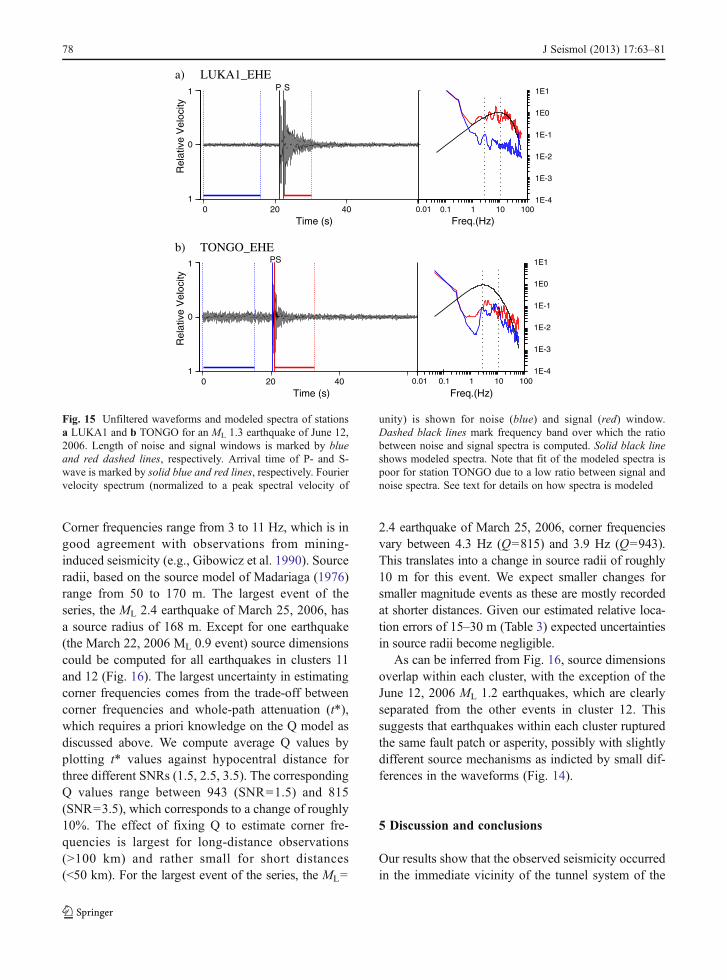
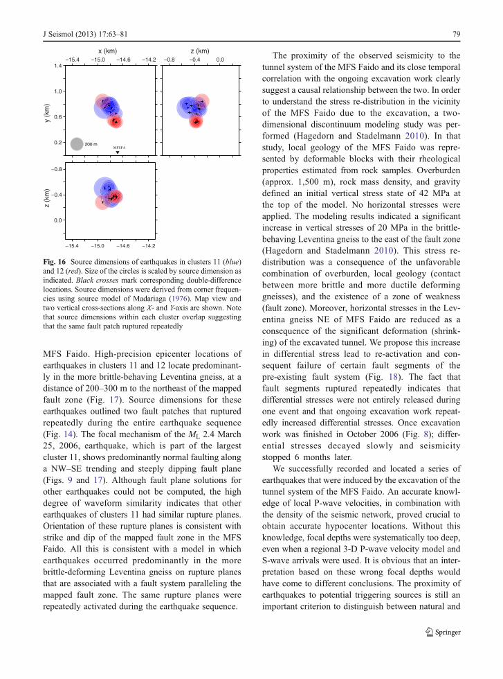
Corner frequencies range from 3 to 11 Hz, which is ingood agreement with observations from mining-induced seismicity (e.g., Gibowicz et al. 1990). Sourceradii, based on the source model of Madariaga (1976)range from 50 to 170 m. The largest event of theseries, the ML 2.4 earthquake of March 25, 2006, hasa source radius of 168 m. Except for one earthquake(the March 22, 2006 ML 0.9 event) source dimensionscould be computed for all earthquakes in clusters 11and 12 (Fig. 16). The largest uncertainty in estimatingcorner frequencies comes from the trade-off betweencorner frequencies and whole-path attenuation (t*),which requires a priori knowledge on the Q model asdiscussed above. We compute average Q values byplotting t* values against hypocentral distance forthree different SNRs (1.5, 2.5, 3.5). The correspondingQ values range between 943 (SNR01.5) and 815(SNR03.5), which corresponds to a change of roughly10%. The effect of fixing Q to estimate corner fre-quencies is largest for long-distance observations(>100 km) and rather small for short distances(<50 km). For the largest event of the series, the ML0
2.4 earthquake of March 25, 2006, corner frequenciesvary between 4.3 Hz (Q0815) and 3.9 Hz (Q0943).This translates into a change in source radii of roughly10 m for this event. We expect smaller changes forsmaller magnitude events as these are mostly recordedat shorter distances. Given our estimated relative loca-tion errors of 15–30 m (Table 3) expected uncertaintiesin source radii become negligible.
As can be inferred from Fig. 16, source dimensionsoverlap within each cluster, with the exception of theJune 12, 2006 ML 1.2 earthquakes, which are clearlyseparated from the other events in cluster 12. Thissuggests that earthquakes within each cluster rupturedthe same fault patch or asperity, possibly with slightlydifferent source mechanisms as indicted by small dif-ferences in the waveforms (Fig. 14).
5 Discussion and conclusions
Our results show that the observed seismicity occurredin the immediate vicinity of the tunnel system of the
1
0
1
Rel
ativ
e V
eloc
ity
1
0
1
Rel
ativ
e V
eloc
ity
0 20 40Time (s)
LUKA1_EHE a)
b)
P S
P S
0.01 0.1 1 10 100
Freq.(Hz)
1E-4
1E-3
1E-2
1E-1
1E0
1E1
0.10.01 1 10 100
Freq.(Hz)
1E-4
1E-3
1E-2
1E-1
1E0
1E1
0 20 40Time (s)
TONGO_EHE
Fig. 15 Unfiltered waveforms and modeled spectra of stationsa LUKA1 and b TONGO for an ML 1.3 earthquake of June 12,2006. Length of noise and signal windows is marked by blueand red dashed lines, respectively. Arrival time of P- and S-wave is marked by solid blue and red lines, respectively. Fouriervelocity spectrum (normalized to a peak spectral velocity of
unity) is shown for noise (blue) and signal (red) window.Dashed black lines mark frequency band over which the ratiobetween noise and signal spectra is computed. Solid black lineshows modeled spectra. Note that fit of the modeled spectra ispoor for station TONGO due to a low ratio between signal andnoise spectra. See text for details on how spectra is modeled
78 J Seismol (2013) 17:63–81
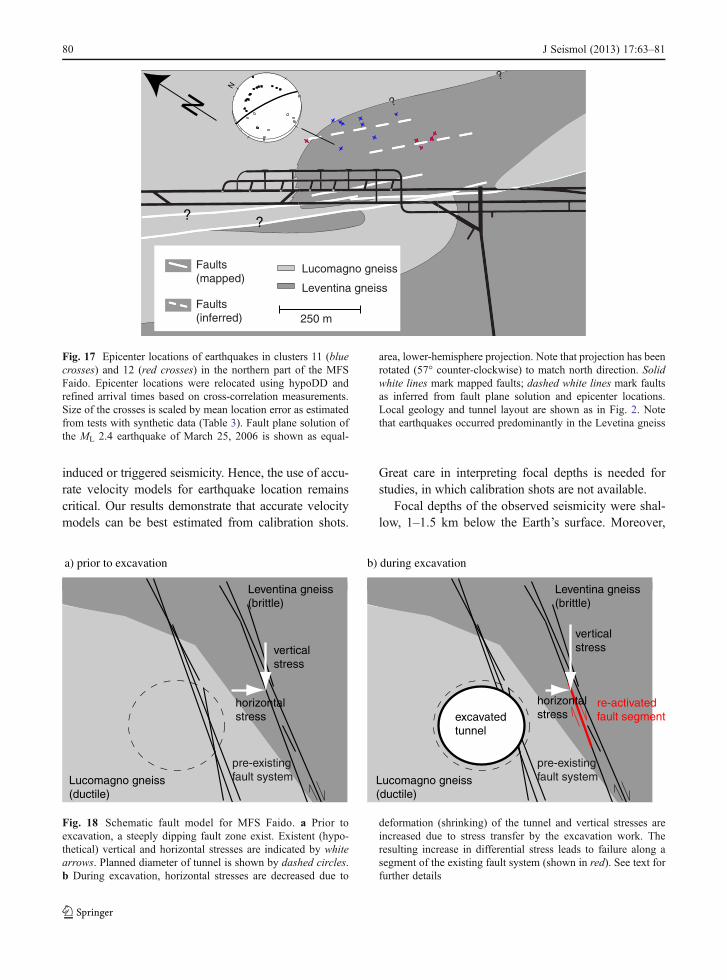
MFS Faido. High-precision epicenter locations ofearthquakes in clusters 11 and 12 locate predominant-ly in the more brittle-behaving Leventina gneiss, at adistance of 200–300 m to the northeast of the mappedfault zone (Fig. 17). Source dimensions for theseearthquakes outlined two fault patches that rupturedrepeatedly during the entire earthquake sequence(Fig. 14). The focal mechanism of the ML 2.4 March25, 2006, earthquake, which is part of the largestcluster 11, shows predominantly normal faulting alonga NW–SE trending and steeply dipping fault plane(Figs. 9 and 17). Although fault plane solutions forother earthquakes could not be computed, the highdegree of waveform similarity indicates that otherearthquakes of clusters 11 had similar rupture planes.Orientation of these rupture planes is consistent withstrike and dip of the mapped fault zone in the MFSFaido. All this is consistent with a model in whichearthquakes occurred predominantly in the morebrittle-deforming Leventina gneiss on rupture planesthat are associated with a fault system paralleling themapped fault zone. The same rupture planes wererepeatedly activated during the earthquake sequence.
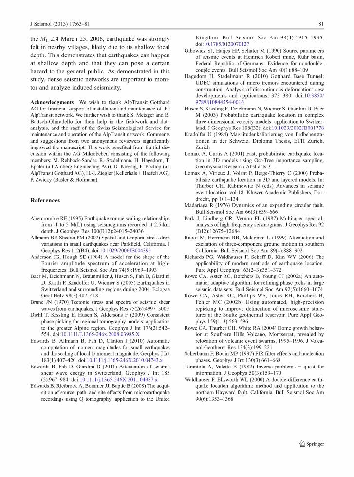
The proximity of the observed seismicity to thetunnel system of the MFS Faido and its close temporalcorrelation with the ongoing excavation work clearlysuggest a causal relationship between the two. In orderto understand the stress re-distribution in the vicinityof the MFS Faido due to the excavation, a two-dimensional discontinuum modeling study was per-formed (Hagedorn and Stadelmann 2010). In thatstudy, local geology of the MFS Faido was repre-sented by deformable blocks with their rheologicalproperties estimated from rock samples. Overburden(approx. 1,500 m), rock mass density, and gravitydefined an initial vertical stress state of 42 MPa atthe top of the model. No horizontal stresses wereapplied. The modeling results indicated a significantincrease in vertical stresses of 20 MPa in the brittle-behaving Leventina gneiss to the east of the fault zone(Hagedorn and Stadelmann 2010). This stress re-distribution was a consequence of the unfavorablecombination of overburden, local geology (contactbetween more brittle and more ductile deforminggneisses), and the existence of a zone of weakness(fault zone). Moreover, horizontal stresses in the Lev-entina gneiss NE of MFS Faido are reduced as aconsequence of the significant deformation (shrink-ing) of the excavated tunnel. We propose this increasein differential stress lead to re-activation and con-sequent failure of certain fault segments of thepre-existing fault system (Fig. 18). The fact thatfault segments ruptured repeatedly indicates thatdifferential stresses were not entirely released duringone event and that ongoing excavation work repeat-edly increased differential stresses. Once excavationwork was finished in October 2006 (Fig. 8); differ-ential stresses decayed slowly and seismicitystopped 6 months later.
We successfully recorded and located a series ofearthquakes that were induced by the excavation of thetunnel system of the MFS Faido. An accurate knowl-edge of local P-wave velocities, in combination withthe density of the seismic network, proved crucial toobtain accurate hypocenter locations. Without thisknowledge, focal depths were systematically too deep,even when a regional 3-D P-wave velocity model andS-wave arrivals were used. It is obvious that an inter-pretation based on these wrong focal depths wouldhave come to different conclusions. The proximity ofearthquakes to potential triggering sources is still animportant criterion to distinguish between natural and
200 m
−0.8
−0.4
0.0
−15.4 −15.0 −14.6 −14.2
0.2
0.6
1.0
1.4
y (k
m)
z (k
m)
−15.4 −15.0 −14.6 −14.2
x (km) z (km)−0.8 −0.4 0.0
MFSFA
Fig. 16 Source dimensions of earthquakes in clusters 11 (blue)and 12 (red). Size of the circles is scaled by source dimension asindicated. Black crosses mark corresponding double-differencelocations. Source dimensions were derived from corner frequen-cies using source model of Madariaga (1976). Map view andtwo vertical cross-sections along X- and Y-axis are shown. Notethat source dimensions within each cluster overlap suggestingthat the same fault patch ruptured repeatedly
J Seismol (2013) 17:63–81 79
induced or triggered seismicity. Hence, the use of accu-rate velocity models for earthquake location remainscritical. Our results demonstrate that accurate velocitymodels can be best estimated from calibration shots.
Great care in interpreting focal depths is needed forstudies, in which calibration shots are not available.
Focal depths of the observed seismicity were shal-low, 1–1.5 km below the Earth’s surface. Moreover,
?
?
?
N? ?
Faults (inferred)
Faults (mapped)
Lucomagno gneiss
Leventina gneiss
N
Fig. 17 Epicenter locations of earthquakes in clusters 11 (bluecrosses) and 12 (red crosses) in the northern part of the MFSFaido. Epicenter locations were relocated using hypoDD andrefined arrival times based on cross-correlation measurements.Size of the crosses is scaled by mean location error as estimatedfrom tests with synthetic data (Table 3). Fault plane solution ofthe ML 2.4 earthquake of March 25, 2006 is shown as equal-
area, lower-hemisphere projection. Note that projection has beenrotated (57° counter-clockwise) to match north direction. Solidwhite lines mark mapped faults; dashed white lines mark faultsas inferred from fault plane solution and epicenter locations.Local geology and tunnel layout are shown as in Fig. 2. Notethat earthquakes occurred predominantly in the Levetina gneiss
Leventina gneiss(brittle)
a) prior to excavation b) during excavation
pre-existing fault system
Leventina gneiss(brittle)
Lucomagno gneiss(ductile)
Lucomagno gneiss(ductile)
pre-existing fault system
re-activated fault segment
vertical stress
horizontalstress
vertical stress
horizontalstress excavated
tunnel
Fig. 18 Schematic fault model for MFS Faido. a Prior toexcavation, a steeply dipping fault zone exist. Existent (hypo-thetical) vertical and horizontal stresses are indicated by whitearrows. Planned diameter of tunnel is shown by dashed circles.b During excavation, horizontal stresses are decreased due to
deformation (shrinking) of the tunnel and vertical stresses areincreased due to stress transfer by the excavation work. Theresulting increase in differential stress leads to failure along asegment of the existing fault system (shown in red). See text forfurther details
80 J Seismol (2013) 17:63–81
the ML 2.4 March 25, 2006, earthquake was stronglyfelt in nearby villages, likely due to its shallow focaldepth. This demonstrates that earthquakes can happenat shallow depth and that they can pose a certainhazard to the general public. As demonstrated in thisstudy, dense seismic networks are important to moni-tor and analyze induced seismicity.
Acknowledgments We wish to thank AlpTransit GotthardAG for financial support of installation and maintenance of theAlpTransit network. We further wish to thank S. Metzger and B.Baitsch-Ghiradello for their help in the fieldwork and dataanalysis, and the staff of the Swiss Seismological Service formaintenance and operation of the AlpTransit network. Commentsand suggestions from two anonymous reviewers significantlyimproved the manuscript. This work benefited from fruitful dis-cussion within the AG Mikrobeben consisting of the followingmembers: M. Rehbock-Sander, R. Stadelmann, H. Hagedorn, T.Eppler (all Amberg Engineering AG), D. Kressig, F. Pochop (allAlpTransit Gotthard AG), H.-J. Ziegler (Kellerhals + Haefeli AG),P. Zwicky (Basler & Hofmann).
References
Abercrombie RE (1995) Earthquake source scaling relationshipsfrom -1 to 5 M(L) using seismograms recorded at 2.5-kmdepth. J Geophys Res 100(B12):24015–24036
Allmann BP, Shearer PM (2007) Spatial and temporal stress dropvariations in small earthquakes near Parkfield, California. JGeophys Res 112(B4). doi:10.1029/2006JB004395
Anderson JG, Hough SE (1984) A model for the shape of theFourier amplitude spectrum of acceleration at high-frequencies. Bull Seismol Soc Am 74(5):1969–1993
Baer M, Deichmann N, Braunmiller J, Husen S, Fah D, GiardiniD, Kastli P, Kradolfer U, Wiemer S (2005) Earthquakes inSwitzerland and surrounding regions during 2004. EclogaeGeol Helv 98(3):407–418
Brune JN (1970) Tectonic stress and spectra of seismic shearwaves from earthquakes. J Geophys Res 75(26):4997–5009
Diehl T, Kissling E, Husen S, Aldersons F (2009) Consistentphase picking for regional tomography models: applicationto the greater Alpine region. Geophys J Int 176(2):542–554. doi:10.1111/J.1365-246x.2008.03985.X
Edwards B, Allmann B, Fah D, Clinton J (2010) Automaticcomputation of moment magnitudes for small earthquakesand the scaling of local to moment magnitude. Geophys J Int183(1):407–420. doi:10.1111/j.1365-246X.2010.04743.x
Edwards B, Fah D, Giardini D (2011) Attenuation of seismicshear wave energy in Switzerland. Geophys J Int 185(2):967–984. doi:10.1111/j.1365-246X.2011.04987.x
Edwards B, Rietbrock A, Bommer JJ, Baptie B (2008) The acqui-sition of source, path, and site effects from microearthquakerecordings using Q tomography: application to the United
Kingdom. Bull Seismol Soc Am 98(4):1915–1935.doi:10.1785/0120070127
Gibowicz SJ, Harjes HP, Schafer M (1990) Source parametersof seismic events at Heinrich Robert mine, Ruhr basin,Federal Republic of Germany: Evidence for nondouble-couple events. Bull Seismol Soc Am 80(1):88–109
Hagedorn H, Stadelmann R (2010) Gotthard Base Tunnel:UDEC simulations of micro tremors encountered duringconstruction. Analysis of discontinuous deformation: newdevelopments and applications, 373–380. doi:10.3850/9789810844554-0016
Husen S, Kissling E, Deichmann N, Wiemer S, Giardini D, BaerM (2003) Probabilistic earthquake location in complexthree-dimensional velocity models: application to Switzer-land. J Geophys Res 108(B2). doi:10.1029/2002JB001778
Kradolfer U (1984) Magnitudenkalibrierung von Erdbebensta-tionen in der Schweiz. Diploma Thesis, ETH Zurich,Zurich
Lomax A, Curtis A (2001) Fast, probabilistic earthquake loca-tion in 3D models using Oct-Tree importance sampling.Geophysical Research Abstracts 3
Lomax A, Virieux J, Volant P, Berge-Thierry C (2000) Proba-bilistic earthquake location in 3D and layered models. In:Thurber CH, Rabinowitz N (eds) Advances in seismicevent location, vol 18. Kluwer Academic Publishers, Dor-drecht, pp 101–134
Madariaga R (1976) Dynamics of an expanding circular fault.Bull Seismol Soc Am 66(3):639–666
Park J, Lindberg CR, Vernon FL (1987) Multitaper spectral-analysis of high-frequency seismograms. J Geophys Res 92(B12):12675–12684
Raoof M, Herrmann RB, Malagnini L (1999) Attenuation andexcitation of three-component ground motion in southernCalifornia. Bull Seismol Soc Am 89(4):888–902
Richards PG, Waldhauser F, Schaff D, Kim WY (2006) Theapplicability of modern methods of earthquake location.Pure Appl Geophys 163(2–3):351–372
Rowe CA, Aster RC, Borchers B, Young CJ (2002a) An auto-matic, adaptive algorithm for refining phase picks in largeseismic data sets. Bull Seismol Soc Am 92(5):1660–1674
Rowe CA, Aster RC, Phillips WS, Jones RH, Borchers B,Fehler MC (2002b) Using automated, high-precisionrepicking to improve delineation of microseismic struc-tures at the Soultz geothermal reservoir. Pure Appl Geo-phys 159(1–3):563–596
Rowe CA, Thurber CH, White RA (2004) Dome growth behav-ior at Soufriere Hills Volcano, Montserrat, revealed byrelocation of volcanic event swarms, 1995–1996. J Volca-nol Geotherm Res 134(3):199–221
Scherbaum F, Bouin MP (1997) FIR filter effects and nucleationphases. Geophys J Int 130(3):661–668
Tarantola A, Valette B (1982) Inverse problems 0 quest forinformation. J Geophys 50(3):159–170
Waldhauser F, Ellsworth WL (2000) A double-difference earth-quake location algorithm: method and application to thenorthern Hayward fault, California. Bull Seismol Soc Am90(6):1353–1368
J Seismol (2013) 17:63–81 81