Millennia of Poverty: If Not Malthusian, Then Why?

Lemin Wu∗

April 11, 2013

Abstract

Living standards were constant for thousands of years before the industrial

revolution. Malthus explained it this way: population grows faster when living

standards rise; therefore, changes in technology alter the density of population

but not the average welfare. This paper challenges Malthus’s explanation of the

constancy and replaces it with the theory of group selection.

Malthusian theory is inadequate because it misses the fact that a dollar’s worth

of diamonds contributes less to survival and reproduction than a dollar’s worth of

grain. Grain is a subsistence commodity and a diamond is a surplus commodity.

The Malthusian force anchors the average level of subsistence, but not that of

surplus. If the surplus sector had grown faster than the subsistence sector, then

living standards could have grown steadily before the industrial revolution, but they

did not. The constancy of living standards thus implies that growth was balanced

between subsistence and surplus, something Malthus did not explain.

To explain the balanced growth, I propose the theory of group selection. Selec-

tion of group characteristics, including culture and technology, goes on by migration

and conquests. Since living standards rise with the ratio of surplus to subsistence,

migrants and invaders usually move from places relatively rich in subsistence to

those relatively rich in surplus. They spread the culture and technology of their

subsistence-rich origin to the surplus-rich destination - the bias of migration fa-

vors the spread of subsistence over that of surplus. Even if surplus cultures and

technologies would develop faster than subsistence ones in a local environment, the

offsetting biased migration balances the two sectors on a global scale. This explains

the constancy of living standards.

My new theory reinterprets why living standards declined after the Agricultural

Revolution and stagnated afterwards, how the Industrial Revolution happened and

where the prosperity of Roman Empire and Song Dynasty came from.

∗University of California, Berkeley. Email: wulm.03@gmail.com; Website: wulemin.weebly.com

1

Acknowledgement

I would like to thank Bradford DeLong, Ronald Lee, Gerard Roland, George Akerlof,

Pranab Bardhan, Martha Olney and Yingyi Qian for exceptional guiding. I also would like

to thank Yang Xie, Dominick Bartelme, Gregory Clark, Maria Coelho, Jeremie Cohen-

Setton, Carola Conces, Jan De Vries, Barry Eichengreen, Sigmund Ellingsrud, Fan Fei,

Simon Galle, Yuriy Gorodnichenko, Joshua Hausman, Sandile Hlatshwayo, Ye Jin, Hash-

mat Khan, Xiaohuan Lan, Peter Lindert, Israel Romen, Changcheng Song, Stephen Sun,

Michael Minye Tang, Holly Wang, Johannes Wieland, Jianhuan Xu, Lei Xu and the

attendants of Berkeley Economic History seminar and Berkeley Macroeconomics and

International economic seminar for thoughtful suggestions and essential encouragement.

2

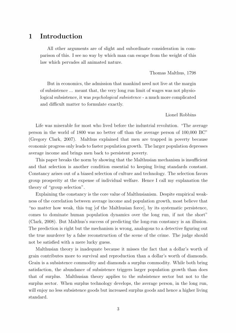
1 Introduction

All other arguments are of slight and subordinate consideration in com-

parison of this. I see no way by which man can escape from the weight of this

law which pervades all animated nature.

Thomas Malthus, 1798

But in economics, the admission that mankind need not live at the margin

of subsistence ... meant that, the very long run limit of wages was not physio-

logical subsistence, it was psychological subsistence - a much more complicated

and difficult matter to formulate exactly.

Lionel Robbins

Life was miserable for most who lived before the industrial revolution. “The average

person in the world of 1800 was no better off than the average person of 100,000 BC”

(Gregory Clark, 2007). Malthus explained that men are trapped in poverty because

economic progress only leads to faster population growth. The larger population depresses

average income and brings men back to persistent poverty.

This paper breaks the norm by showing that the Malthusian mechanism is insufficient

and that selection is another condition essential to keeping living standards constant.

Constancy arises out of a biased selection of culture and technology. The selection favors

group prosperity at the expense of individual welfare. Hence I call my explanation the

theory of “group selection”.

Explaining the constancy is the core value of Malthusianism. Despite empirical weak-

ness of the correlation between average income and population growth, most believe that

“no matter how weak, this tug [of the Malthusian force], by its systematic persistence,

comes to dominate human population dynamics over the long run, if not the short”

(Clark, 2008). But Malthus’s success of predicting the long-run constancy is an illusion.

The prediction is right but the mechanism is wrong, analogous to a detective figuring out

the true murderer by a false reconstruction of the scene of the crime. The judge should

not be satisfied with a mere lucky guess.

Malthusian theory is inadequate because it misses the fact that a dollar’s worth of

grain contributes more to survival and reproduction than a dollar’s worth of diamonds.

Grain is a subsistence commodity and diamonds a surplus commodity. While both bring

satisfaction, the abundance of subsistence triggers larger population growth than does

that of surplus. Malthusian theory applies to the subsistence sector but not to the

surplus sector. When surplus technology develops, the average person, in the long run,

will enjoy no less subsistence goods but increased surplus goods and hence a higher living

standard.

3

The division of surplus and subsistence is universal. For any commodity, calculate

its marginal effects, in per capita terms, on the growth rate of population and on an

average person’s utility. Define the ratio of the marginal population growth rate to the

marginal utility as the “subsistence index”. The index measures the demographic effect

of the commodity relative to its hedonistic value.

Grain has a higher subsistence index than diamonds, therefore grain is a relative

subsistence. In the same way, in pre-modern England, agricultural products are a sub-

sistence commodity relative to manufacture products; arables relative to pastures; and

barley and oats relative to wheat. We can order all the commodities by their subsistence

index. The order is complete and transitive so that we can divide the whole spectrum

into two groups. One forms the surplus sector and the other the subsistence sector. My

theory thus differs from the Malthusian model by having two sectors instead of one.

Changes of productivity in different sectors affect population growth differently. The

use of a better fertilizer feeds more people; but a smarter diamond cut does not. Progress

in surplus technology has little effect on population growth, so that the Malthusian force

cannot hinder the growth of average surplus.

Neither can it hinder the growth of living standards, because living standards depend

on average surplus: they are a function of average surplus and average subsistence. Since

average subsistence is fixed by the Malthusian force, average surplus solely determines

the equilibrium living standards.

Average surplus is equal to the ratio of surplus to subsistence multiplied by average

subsistence:Surplus

Population=

Surplus

Subsistence× Subsistence

Population.

Now that the last term - the average subsistence - is fixed, the living standards depend

on the ratio of surplus to subsistence only. The ratio varies from place to place. The

larger it is, the higher the living standards will be.

In the long run, living standards could have grown steadily. It would have happened

as long as surplus had grown faster than subsistence; and the Malthusian force would have

had no way to check it. The relative growth of surplus would even create a momentum

for itself: the higher the living standards, the larger the demand for surplus is - surplus

is a luxury and its demand rises with income - and the rise in surplus consumption would

further increase the living standards. But nothing of this sort ever happened before the

industrial revolution. The lack of growth implies that surplus had grown at the same rate

as subsistence. The puzzle of Malthusian constancy is essentially a puzzle of balanced

growth, which Malthus did not explain.

To explain the puzzle, I propose the theory of group selection. Selection takes place

in the spread of subsistence cultures and technologies. Subsistence technologies are those

methods of production that raise subsistence productivity more than they raise surplus

4

productivity. A subsistence technology lowers the ratio of surplus to subsistence. As a

result, it causes the equilibrium living standards to decline and drives the people who

adopt it to migrate abroad for a higher living standard. In contrast, a surplus technology

raises the living standards and attracts immigration. The natives who learn the surplus

technology are reluctant to go to the “gentiles” to spread the “gospel”. Therefore, mi-

gration is biased from the subsistence-rich regions to the surplus-rich regions. It spreads

subsistence technologies faster than surplus technologies.

Ironically, subsistence technologies get spread faster by making people worse off. The

paradox arises because individuals do not take into account the effect of their behavior on

group welfare. An 18th-century Irish peasant would not refrain from cultivating potato -

a crop imported from America - by foreseeing the misery of a denser population. Even if

he refrained, he could not stop the other peasants from tilling potato and bearing more

children. Everyone seeks a better life; each pursues her own agenda; but collectively, they

evoke “the tragedy of the commons”.

If there had been no such biased migration, then living standards would have grown

steadily as long as surplus productivity grows faster than subsistence productivity. How-

ever, migration offsets the local advantage of surplus growth by the global advantage

of subsistence spread. Left alone, every place would have prospered; but globally, they

are held in check by the interlock of selection - migration selects technologies by their

surplus-subsistence characteristics. Selection picks the poverty-stricken and makes their

lifestyle prevail.

The same logic extends from technology to culture. Culture is the social norm that

sorts out winners and losers. Winners gain status, respect and the favor of the other sex.

To be such a winner, people show off in galleries and theaters, on catwalks and boxing

rings. These surplus cultures divert resources from supporting a larger population to

promoting one’s relative status in society. In other words, if we define the growth rate

of population as the group fitness, surplus promotes individual fitness at the expense of

group fitness.

The demand for surplus is the individuals’ Nash equilibrium strategy, commonly held

and genetically programmed, that survives natural selection and makes us who we are. No

art or music would be possible but for the demand for surplus; and none would demand

surplus but for the conflict of interest between individual and group. By the measure of

fitness, surplus consumption is a prisoner dilemma; yet by the measure of utility, it is a

blessed curse.

Surplus culture makes people better off. It requires one to spend more on surplus

and less on subsistence. As a result, population is lower than if the surplus culture is

absent. In the long run, the average subsistence will hardly be affected but the average

surplus will become larger. Overall, surplus is “socially free”: when people desire more,

5

they receive more in the end; and they do not have to pay for it by sacrificing average

subsistence. The people who pay for the surplus are those who would have been born.

However, surplus culture has a limit. Hedonism is checked by migration and invasion.

It makes a people vulnerable to greedy neighbors: the high surplus attracts the invaders;

and the low subsistence means fewer people to defend it. This is why the “arms race” of

conspicuous consumption does not spiral out of control. Locally, the race might escalate;

globally, it is suppressed by group selection. I call the process group selection because

culture is a group characteristic. Culture affects the fate of the group; and by doing so, it

decides its own fate. By suppressing surplus culture, group selection traces out a path of

balanced growth. Along the path, mankind were trapped for tens of thousands of years

in the constancy of living standards.

In explaining the constancy, I develop my theory in two steps. First, I raise the

puzzle of balanced growth by the division of surplus and subsistence; then I use the

theory of group selection to solve the puzzle. I try to answer Malthus’s question: why

living standards had stagnated for such a long time.

Beyond explaining the constancy, the theory is rich with other implications. Consider

the ancient market economies, such as Roman empire and Song dynasty. The classical

theory portrays their prosperity as an ephemeral carnival, a temporary “disequilibrium” of

the Malthusian model. In contrast, my theory attributes the prosperity to the persistent

effect of long peace, wise governance, light tax and market economy. These “Smithian”

factors boost surplus productivity more than subsistence productivity. As a result, these

policies improve equilibrium living standards not only in Solow’s era but also in Malthus’s

time. Roman and Song civilizations later collapsed not because their population exceeded

the capacity of land but because the neighboring groups invaded and conquered them. In

particular, Roman economy was exhausted by the wars with Sassanid Empire; and the

city of Rome was sacked by the Visigoth immigrants.

The theory also addresses the twin puzzles of the agriculture revolution - why living

standards declined after men took up agriculture and why agriculture swept the world

despite its negative effect on living standards. In light of my theory, agriculture is a

subsistence technology. It lowers the equilibrium living standards and spreads fast by

biased migration.

Last but not the least, the theory puts the industrial revolution into perspective.

Explosive changes such as the appearance of agriculture, the rise of Islam, the march of

Genghis Khan and the industrial revolution all share the same pattern: some surplus

turns into subsistence - a local trait attempts global dominance by winning over group

selection from a constraint into a boost. These phenomena are called surplus explosions,

which I explore in detail in the third chapter of my dissertation.

6

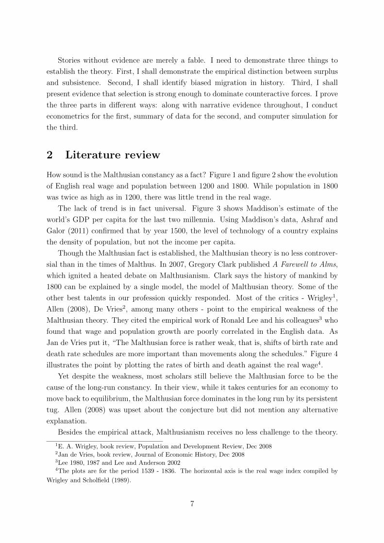
Stories without evidence are merely a fable. I need to demonstrate three things to

establish the theory. First, I shall demonstrate the empirical distinction between surplus

and subsistence. Second, I shall identify biased migration in history. Third, I shall

present evidence that selection is strong enough to dominate counteractive forces. I prove

the three parts in different ways: along with narrative evidence throughout, I conduct

econometrics for the first, summary of data for the second, and computer simulation for

the third.

2 Literature review

How sound is the Malthusian constancy as a fact? Figure 1 and figure 2 show the evolution

of English real wage and population between 1200 and 1800. While population in 1800

was twice as high as in 1200, there was little trend in the real wage.

The lack of trend is in fact universal. Figure 3 shows Maddison’s estimate of the

world’s GDP per capita for the last two millennia. Using Maddison’s data, Ashraf and

Galor (2011) confirmed that by year 1500, the level of technology of a country explains

the density of population, but not the income per capita.

Though the Malthusian fact is established, the Malthusian theory is no less controver-

sial than in the times of Malthus. In 2007, Gregory Clark published A Farewell to Alms,

which ignited a heated debate on Malthusianism. Clark says the history of mankind by

1800 can be explained by a single model, the model of Malthusian theory. Some of the

other best talents in our profession quickly responded. Most of the critics - Wrigley1,

Allen (2008), De Vries2, among many others - point to the empirical weakness of the

Malthusian theory. They cited the empirical work of Ronald Lee and his colleagues3 who

found that wage and population growth are poorly correlated in the English data. As

Jan de Vries put it, “The Malthusian force is rather weak, that is, shifts of birth rate and

death rate schedules are more important than movements along the schedules.” Figure 4

illustrates the point by plotting the rates of birth and death against the real wage4.

Yet despite the weakness, most scholars still believe the Malthusian force to be the

cause of the long-run constancy. In their view, while it takes centuries for an economy to

move back to equilibrium, the Malthusian force dominates in the long run by its persistent

tug. Allen (2008) was upset about the conjecture but did not mention any alternative

explanation.

Besides the empirical attack, Malthusianism receives no less challenge to the theory.

1E. A. Wrigley, book review, Population and Development Review, Dec 20082Jan de Vries, book review, Journal of Economic History, Dec 20083Lee 1980, 1987 and Lee and Anderson 20024The plots are for the period 1539 - 1836. The horizontal axis is the real wage index compiled by

Wrigley and Scholfield (1989).

7

Figure 1: English real wage, 1200 - 1800 (1860=100)

Figure 2: English population, 1200 - 1800 (million)

Figure 3: World per capita GDP 1-2001 AD, in 1990 dollars

8

Figure 4: Wrigley and Schofield’s real wage explains the birth and death rates weakly.

The critics are concerned with Malthus’s failure to capture the modern growth. Scholars

in the 19th century5 had noticed the potential of technological improvement to outpace

the population growth. They also forsaw the possibility of “moral restraint”, that people

might refrain from reproduction voluntarily.

Today’s theorists have a different agenda. They attempt to reconcile the Malthu-

sian constancy with modern growth by endogenizing the acceleration of productivity

growth.6 These models unanimously presumed the Malthusian mechanism to be the

cause of Malthusian constancy. They described how the shackle of Malthusian forces was

finally broken; but they never asked whether the binding shackle was truly Malthusian

or not.

I propose this question. The question is inevitable in a two-sector Malthusian model.

Rudimentary two-sector models did occasionally appear. Davies’s (1994) paper on Gif-

fen goods had beef and potato. Taylor’s (1998) classic on Easter island had food and

manufactures. Two-sector thinking also permeated empirical studies such as Broadberry

and Gupta (2005), which used the ratio of silver-grain wages to proxy for the relative

productivity of tradable goods. Unfortunately, the researchers never took a further step

to explore the long-run implication, that a directional change in production structure

could disturb the constancy of living standards.

This paper explores the long-run implications of the two-sector models. It turns out

I have to face a new puzzle, the puzzle of balanced growth, which I explain with the

theory of group selection. In the past decade, Bowles and Gintis7 revived the idea of

group selection in economic literature, asking why the cooperative traits got rooted in

5Malthus (5th ed., 1817/1963), Everett (1826), Carey (1840) and Engels.6Simon and Steinmann (1991), Jones (2001), Hansen and Prescott (2002), Galor and Weil (2002) and

Galor and Moav (2002), among many others.7Bowles and Gintis (2002) and Bowles (2006). Their work is summarized in the new book, A Coop-

erative Species: Human Reciprocity and Its Evolution (Bowles and Gintis 2011).

9

human nature, though they seem to conflict with individual fitness. The old label of

pseudo-science on group selection is gone. Now theorists have found many ways for

group selection to have an impact. In my theory, selection happens among the multiple

equilibria, so it is compatible with Nash criterion.

A caveat is that the notion of group selection in this paper is not genetic. My theory is

different from Clark’s idea in A Farewell to Alms. While Clark attributes the Industrial

Revolution to natural selection, I explain the Malthusian stagnation with selection of

culture and technology.

Levine and Modica (2011) is the closest research to mine. They use the idea of group

selection to challenge the Malthusian prediction of persistent poverty. Though we share

the same solution to Malthusian economics, we approach the issue in different ways and

reach different conclusions. They treat the constancy not as a solid fact to explain but as a

false prediction to challenge. They do not distinguish surplus and subsistence, but instead

focus on the allocation of resources between people and authority. Their equilibrium is

the maximization of resources the authority controls to engage in wars; while mine is

the balance of growth and constancy of living standards. My thesis is complementary to

theirs. Together we show how the idea of group selection can change our view on the part

of history which economists used to think is explained by a single model of Malthusian

theory.

3 Models

3.1 The mathematical definition of surplus

Surplus is what contributes little to population, relative to its contribution to utility.

Suppose an isolated group of homogeneous people. The level of population isH. There

are M kinds of commodities, j = 1, 2, ...,M . The representative agent’s consumption is

E ∈ RM+ . Within the choice set, he maximizes a utility function that is differentiable and

strictly increasing:

maxE∈C(N)

U(E)

The choice set C shrinks when population rises: ∀H1 < H2, C(H1) ⊃ C(H2).

Let the growth rate of population depend on the average consumption E,

H

H= n(E)

Now assume the population growth rate n(E) is differentiable and strictly increasing.

There exist a set S on which population does not change, n(S) = 0. Call it the constant

population set. When population stabilizes, the economy returns to its equilibrium on

the constant population set.

10

When U(E) is not a transformation of n(E), there must exist some bundle of con-

sumption E, at which one commodity is more of subsistence than another, i.e., ∃j1, j2 ∈{1, 2, ...,M} such that

∂n(E)∂Ej1

∂U(E)∂Ej1

>

∂n(E)∂Ej2

∂U(E)∂Ej2

Compared with j2, commodity j1 marginally contributes more to population growth than

to individual utility. It makes j1 a subsistence commodity relative to j2. In fact, we can

define a subsistence index for each commodity. ∀E ∈ RM+ , ∀j ≤ M , commodity j’s

subsistence index at E is∂n(E)∂Ej

∂U(E)∂Ej

Order the indices of all commodities from small to large. Then we get a spectrum of

commodities from surplus to subsistence. I then divide the spectrum into two groups,

the surplus sector and the subsistence sector.

The bottom line is, we can always distinguish surplus and subsistence as long as U(E)

is not a transformation of n(E). Later I shall discuss why the condition is important.

3.2 The two-sector Malthusian model

Figure 5 illustrates the above algebra. It features the representative agent’s consump-

tion space. In addition to the conventional indifference curve and production possibility

frontier, the diagram has a “constant population curve” (figure 5B): population stays

constant if consumption bundle is on the curve. If consumption lies to the left of the

curve - people consume less than what reproduction requires - population declines; if to

the right, population rises.

Figure 5: Adding the constant population curve

11

The change of population is reflected in the shift of production possibility frontier:

when population declines, the frontier expands, for each person is endowed with a larger

choice set; when population rises, the frontier contracts. The choice set decreases with

population because Malthusian economies are characterized by diminishing returns to

labor. There are diminishing returns to labor because land is an important factor of

production and its supply is inelastic.

Without loss of generality, I assume the expansion and contraction of the production

possibility frontier to be proportional between the sectors. In other words, the production

structure is independent of the size of population.8

The constant population curve crosses the indifference curve from above because sub-

sistence is more important to population growth than surplus.9 The curve is not perfectly

vertical because surplus can affect population growth as well, though the effect is smaller

than that of subsistence.

The equilibrium must lie on the constant population curve. As figure 6 illustrates,

if the economy deviates rightward, the temporary affluence raises the growth rate of

population. As population grows, individuals’ choice set contracts backward, until the

economy returns to the constant population curve.

Figure 6: The equilibrium is on the constant population curve.

Now a surplus technology can improve the equilibrium living standards. The sur-

8It would be an interesting extension to assume subsistence is more labor-intensive than surplus. But

I will stick to the simplifying assumption to highlight the effect of interest.9The definition of surplus and subsistence dictates the way the constant population curve crosses the

indifference curve. If we label subsistence as A and surplus as B,

∂n(E)∂EA

∂U(E)∂EA

>

∂n(E)∂EB

∂U(E)∂EB

=⇒∂n(E)∂EA

∂n(E)∂EB

>

∂U(E)∂EA

∂U(E)∂EB

i.e., MRSn > MRSU

so the constant population curve is steeper than the indifference curve.

12

plus technology expands the production possibility frontier vertically (figure 7A). After

population adjusts, the economy returns to the constant population curve in the end

(figure 7B). The new equilibrium (E ′′) is above the old one (E) because the production

possibility frontier becomes steeper after the surplus technology shock.

Figure 7: A surplus technology improves the equilibrium living standards.

In contrast, a subsistence technology causes living standards to decline. In figure 8A,

the production possibility frontier expands horizontally as subsistence sector expands.

The abundance of subsistence triggers the rise of population. After the economy returns

to the constant population curve, the new equilibrium stays below the old one, because the

production possibility frontier becomes flatter by the influence of subsistence technology.

In the long run, what matters for living standards is not the size but the shape of the

production possibility frontier.

Figure 8: A subsistence technology lowers the equilibrium living standards.

13

Culture affects the equilibrium as well. Suppose there appears a surplus culture.

It tilts the indifference curve into a flatter one (figure 9A). By trading subsistence for

surplus, population undergoes a gradual decline. But when the adjustment is over, the

remaining population enjoy a higher equilibrium living standard than in the old days

(figure 9B).

Figure 9: The surplus culture improves the equilibrium living standards.

The above results seem to suggest that a more surplus-oriented production structure is

always associated with a higher living standard; and so is social preference. Unfortunately,

exception exists: figure 10 shows the scenario where a surplus economy turns out to have

a lower living standard.

Figure 10: Counterexample: E1 has a steeper PPF but a lower living standard.

The exceptions are caused by multiple equilibria. In appendix A.3, I prove the follow-

ing theorems by a theoretical detour that avoids the ambiguity of multiple equilibria10:

10Appendix A.2 lists the assumptions I make.

14

Theorem 1 (First Production Structure Theorem) For an economy on a stable

equilibrium, a positive surplus technology shock always improves equilibrium living stan-

dards.

Theorem 2 (Second Production Structure Theorem) If the subsistence is not a

Giffen good, an economy of a more surplus-oriented production structure always has higher

equilibrium living standards, other things being equal.

Theorem 3 (First Free Surplus Theorem) For an economy on a stable equilibrium,

a surplus culture always improves equilibrium living standards.

Theorem 4 (Second Free Surplus Theorem) If the subsistence is not a Giffen good,

an economy of a more surplus-oriented social preference always has higher equilibrium

living standards, other things being equal.

Thus, we establish two comparative statics - culture and technology, which are missing

in Malthusian theory. Moreover, the framework works equally well with the old compar-

ative statics that the classical model has covered. When disease environment worsens,

or war becomes more frequent, or people marry later or give birth to fewer, the con-

stant population curve will shift rightward: each bundle of consumption is now related

to a lower rate of population growth (figure 11A). The decline of population expands

the choice set of an average person, so that the new equilibrium provides a higher living

standard than the old one (figure 11B) - the framework preserves the merit of the classical

theory.

Figure 11: The comparative statics of disease, war and fertility strategy

15

3.3 The key different assumption

Malthus made a lot of simplifying assumptions. I differ by relaxing only one of them.

It turns out the assumption I relax is a crucial one. Relaxing it, Malthus would have

predicted a different pattern of living standards growth.

Malthus’s prediction of constancy depends on his implicit assumption that the utility

function U is an increasing transformation of the population growth rate n. In the

diagram, it means that the constant population curve coincides with the indifference

curve.

If so, a surplus technology cannot affect the equilibrium living standards (figure 12).

After a surplus shock, when the economy comes back to the constant population curve

(figure 12C), the new equilibrium has the same level of utility as the old one. This is

because the indifference curve coincides with the constant population curve. As the new

equilibrium falls on the constant population curve, it falls on the same indifference curve

as well (figure 12C).

Figure 12: The Malthusian model as a special case

This is why the classical model predicts the constancy of living standards. If the

constant population curve does not cross the indifference curve, the two sectors can

be reduced into one sector. Malthusian theory is the special case that assumes away

the difference of demographic effect between commodities, assumes away the crossing of

curves, and assumes away the conflict of reproductive interest between individual and

group.

The reproductive conflict between individual and group is the fundamental reason why

the curves cross. In essence, the constant population curve is a curve of iso-group fitness,

along which the group achieves a certain rate of population growth. In parallel, the

indifference curve is a curve of iso-individual fitness: millions of years’ natural selection

16

programs the preference system to maximize the personal chance of reproduction. What

pleases is usually what benefits - it benefits the individual but not necessarily the group.

So the indifference curve is a close approximation of an iso-individual-fitness curve.

The conflict between group fitness and individual utility - which is manifest in the

crossing - is driven by the conflict of fitness between group and individual. Such a conflict

prevails in biology as well as in culture. As sure as the fitness conflict persists, the curves

always cross each other; and the division of surplus and subsistence is a perpetual human

condition.

3.4 The baseline model

The geometric model has presented three comparative statics. All of them can be cap-

tured by a single formula in the following algebraic model.

Let the representative agent maximize a Cobb-Douglas utility function that has con-

stant returns to scale on her subsistence consumption x and surplus consumption y.

U(x, y) = x1−βyβ (1)

Constant returns to scale makes it meaningful to calculate the growth rate of utility.

Utility doubles when consumption doubles.

Specify the subsistence production function as X = AL1−γAA HγA

A and the surplus

production function as Y = BL1−γBB HγB

B . LA and LB are the land used in subsistence

and surplus production. Their sum equals to total endowment of land, LA+LB = L. HA

and HB are the labor employed in subsistence and surplus production. Their sum equals

the total population, HA +HB = H.

To ensure the independence of production structure from the level of population, I

impose the following assumption.

Assumption 1 γA = γB ≡ γ < 1.

I assume γA = γB so that population growth affects surplus and subsistence production

in proportion. γA and γB are smaller than one because diminishing returns to labor is a

central feature of Malthusian economies.

Since the population is homogeneous, assume that

Assumption 2 Each person gets an equal share of social output.

Under assumption 2, by maximizing utility under the land and labor constraint, we

can derive the average surplus and average subsistence:

x = A(1− β)

(H

L

)γ−1

(2)

y = Bβ

(H

L

)γ−1

(3)

17

Substitute equation 2 and equation 3 into U = x1−βyβ. The level of utility is

U = A

(H

L

)γ−1(B

A

)β(1− β)1−βββ (4)

Since A(H/L)γ−1(1−β) = x (equation 2), we can alternatively express U as a function

of x, A and B.

U = x

(B

A

)β (β

1− β

)β(5)

The economy converges to equilibrium by the adjustment of population level. Since

there is no migration for the isolated economy, the net growth rate of population gH must

be equal to the natural growth rate of population n. For simplicity, assume n depends

on the average subsistence only.

Assumption 3 gH ≡ H/H = n = δ(lnx− ln x) and δ > 0.

where x is the level of average subsistence at which population keeps constant. The as-

sumption implies a vertical constant population curve - population growth is independent

of average surplus. The equilibrium of the isolated economy satisfies the condition x = x.

Therefore, in the equilibrium

Proposition 1

UE = x

(B

A

)β (β

1− β

)β(6)

The equilibrium level of utility increases with B/A, β and x.

The formula captures three comparative statics. The equilibrium utility can rise for three

reasons:

1. A rise in the ratio of surplus to subsistence, i.e. B/A rises.

2. A rise in the social preference for surplus, i.e. β rises.

3. A rise in the required consumption for population balance, i.e. x rises.

3.5 The puzzle of balanced growth and its explanations

The equilibrium utility increases with the ratio of surplus to subsistence. It implies that

living standards would have grown steadily if the growth rate of surplus had exceeded

that of subsistence. To see this, let A grow at the rate of gA and B grow at gB. If

gB > gA, what will happen to the growth rate of utility, gU?

First we need a utility formula that relates U to A and B. We cannot use the formula

of equilibrium utility (equation 6) because the continuous progress of technology pulls

the economy slightly away from the equilibrium state, x = x. Therefore we turn to

equation 4, which applies to all scenarios.

18

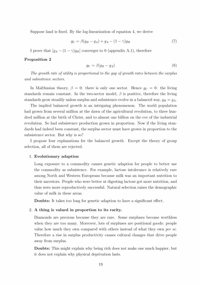
Suppose land is fixed. By the log-linearization of equation 4, we derive

gU = β(gB − gA) + gA − (1− γ)gH (7)

I prove that [gA − (1− γ)gH ] converges to 0 (appendix A.1), therefore

Proposition 2

gU = β(gB − gA) (8)

The growth rate of utility is proportional to the gap of growth rates between the surplus

and subsistence sectors.

In Malthusian theory, β = 0: there is only one sector. Hence gU = 0: the living

standards remain constant. In the two-sector model, β is positive, therefore the living

standards grow steadily unless surplus and subsistence evolve in a balanced way, gB = gA.

The implied balanced growth is an intriguing phenomenon. The world population

had grown from several million at the dawn of the agricultural revolution, to three hun-

dred million at the birth of Christ, and to almost one billion on the eve of the industrial

revolution. So had subsistence production grown in proportion. Now if the living stan-

dards had indeed been constant, the surplus sector must have grown in proportion to the

subsistence sector. But why is so?

I propose four explanations for the balanced growth. Except the theory of group

selection, all of them are rejected.

1. Evolutionary adaption

Long exposure to a commodity causes genetic adaption for people to better use

the commodity as subsistence. For example, lactose intolerance is relatively rare

among North and Western Europeans because milk was an important nutrition to

their ancestors. People who were better at digesting lactose got more nutrition, and

thus were more reproductively successful. Natural selection raises the demographic

value of milk in these areas.

Doubts: It takes too long for genetic adaption to have a significant effect.

2. A thing is valued in proportion to its rarity.

Diamonds are precious because they are rare. Some surpluses become worthless

when they are too many. Moreover, lots of surpluses are positional goods: people

value how much they own compared with others instead of what they own per se.

Therefore a rise in surplus productivity causes cultural changes that drive people

away from surplus.

Doubts: This might explain why being rich does not make one much happier, but

it does not explain why physical deprivation lasts.

19

3. Constant returns to scale

In a dynamic system such as

At+1 = FA(At, Bt)

Bt+1 = FB(At, Bt)

if functions FA and FB have constant returns to scale, A and B will grow in balance

on a stable path (Samuelson and Solow, 1953).

Doubts: Growth is about the generation of ideas. The theorem Samuelson and

Solow proved is not directly applicable to idea generation. There is no obvious

reason why there should be constant returns to scale in the context of surplus and

subsistence growth.

4. Group selection

I cannot reject this hypothesis. The rest of the paper will elaborate how group

selection works, why it causes constancy and what the evidence is for its relevance.

3.6 The model of source-sink migration

How does group selection work? As previously, before using algebra, I will first provide

a geometric model to highlight the intuition.

Suppose there is a sea of identical villages. All start at the equilibrium state in the

beginning (figure 13A). Assume that people migrate freely but never trade across borders.

I assume there is no trade because trade substitutes migration. If people of different

regions face the same relative price of surplus to subsistence, the Malthusian force will

make them choose the same bundle of consumption. Then there would be no need to

migrate. But when trade has a cost, the relative price will differ and migration will

emerge. In the ancient world, trade was never big enough to wipe out the difference of

lifestyle between the nomadic zones and the arable zones. The nomadic invasion and

immigration to the arable zones were a response to the difference of living standards. So

I can relax the assumption of no trade and introduce trade cost without affecting the

qualitative results. I assume the extreme case of no trade only to simplify the analysis.

The assumption is not crucial.

Suppose one of the villages discovers a new way to mine for diamonds. Thanks to the

surplus technology, its production possibility frontier expands vertically (figure 13B). If

migration were forbidden, the diamond village would end up with a higher living standard.

However, free migration equalizes the level of utility between the diamond village and

the others (figure 13C). With a steeper production possibility frontier tangent with the

same indifference curve, the diamond village stays to the left of the constant population

20

Figure 13: Difference of production structure causes source-sink migration.

curve - its death rate is higher than the birth rate. But the natural decrease of population

does not expand the production possibility frontier because the under-reproduction is

filled up by the continuous immigration from the other villages. The pattern lasts as long

as the relative price of surplus to subsistence differs between the villages. The diamond

village becomes a demographic sink and the surrounding villages serve as a demographic

source.

A similar pattern holds for regions that share the same production structure but

differ in social preference. Again, start with the identical villages at the equilibrium state

(figure 14A). Suppose somehow in one of the villages, girls begin to ask for more diamonds

from their suitors. As a result, the indifference curve becomes flatter (figure 14B): people

trade grain for diamonds. If the diamond village were isolated from the rest of world, the

girls would earn what they demand for free: in the long run, the average consumption of

grain would barely change.

But when migration is costless, the difference of social preference causes a similar

pattern of source-sink migration. The outsiders will not migrate in the beginning. They

will wait for the population of the diamond village to decline, from E ′ to E ′′ (figure 14C).

At E ′′, utility equalizes across the border, which triggers a continuous flow of immigration.

From then on, the diamond village stays to the left of the constant population curve -

the death rate is higher than the birth rate and the gap is met by the immigrants.11

The craze for diamonds will not last forever in the diamond village. The constant

flood of immigrants will dilute the diamond culture. This is the fate of most fads and

fashion. The arms race of conspicuous consumption is constrained not by the Malthusian

force, but by group selection, in the form of source-sink migration.

11The migrants are assumed to keep their old preference. If instead they convert to new culture, the

diagram will be slightly different but the source-sink pattern still remains.

21

Figure 14: Difference of culture causes source-sink migration.

Figure 15: The source-sink migration after a subsistence cultural shock

22

On the contrary, a subsistence culture can rise to global dominance by sending out

emigration (figure 15). Take monogamy as an example. Biologically speaking, the elites

would do better under polygamy, and they have the strength as well as the incentive to

bolster it. Yet most of us live in a monogamous society because monogamy is a subsistence

culture: by imposing equality of sexual opportunity, it shifts importance from attracting

the mates to feeding the children, from a surplus activity to a subsistence activity. The

local elites’ incentive and ability pale in the comparison with the power of group selection.

3.7 Selection against surplus growth

The above model geometrically describes how migration is biased to favor the spread of

subsistence culture and technology. Following the same intuition and setup, this section

provides two algebraic models. The first one shows how a single region’s surplus growth is

constrained when it is set against a sea of subsistence regions. The second model derives

the path of global average utility in the case of two regions. Assuming the same β across

regions, the models deal with the selection of technology but not the selection of culture;

the results could be easily extended to the cultural selection.

3.7.1 A sea-of-villages model

Suppose there is a sea of identical villages in the beginning. For each of them, the baseline

model specifies the utility and production functions as well as the population dynamics.

Suppose one of the villages differs from the others by having a different path of surplus

growth. In particular, all the other villages have a constant level of subsistence technology

A′ and a constant level of surplus technology B′, while that single village - though having

the same constant level of subsistence technology A∗ = A′ - has a variable level of surplus

technology B∗ that tends to grow at a constant rate g if unconstrained by immigration.

We call that village the surplus village and the others the subsistence villages.

When B∗ exceeds B′, the difference of production structure will trigger source-sink

migration. If the immigrants influence the technology of the surplus village, how will B∗

evolve? Can biased migration dominate the growth tendency of B∗?

First, we need the assumption of no trade and free migration to determine the migra-

tional equilibrium.12

Assumption 4 Trade is forbidden across the villages but migration is costless. Free

migration equalizes the level of utility between the surplus village and the subsistence

villages, U∗ = U ′.

12Trade cost can be introduced without affecting the qualitative results. In the beginning of section 3.6,

I have discussed the reasons for the assumption.

23

By equation 5, the equality U∗ = U ′ means

x∗(B∗

A∗

)β (β

1− β

)β= x′

(B′

A′

)β (β

1− β

)βwhere x∗ and x′ are the average consumption of subsistence in the surplus village and

the subsistence villages.

The equation can be rearranged into the following:

lnx∗ − lnx′ = −β[ln

(B∗

A∗

)− ln

(B′

A′

)](9)

With free migration, the net emigration rate m is equal to the natural growth rate

of population n, which in turn depends on the average subsistence x, n = δ(lnx∗ − ln x)

(assumption 3). In particular, for the surplus village,

m = n = δ(lnx∗ − ln x) (10)

Here x is the level of average subsistence that keeps the population in natural balance.

Since δ > 0 and x∗ < x, m is negative: migrants move into the surplus region. As

the effect of emigration is negligible on each of the subsistence villages, the subsistence

villages have the equilibrium level of average subsistence, i.e. x′ = x.

Denote s∗ ≡ ln(B∗/A∗) and s′ ≡ ln(B′/A′). Substituting x′ = x and equation 9 into

equation 10, we arrive at

Proposition 3

m = −βδ(s∗ − s′) (11)

The emigration rate is proportional to the difference of production structures. s measures

a region’s ratio of surplus to subsistence. Having a higher ratio of surplus to subsistence

than the neighboring regions causes net immigration.

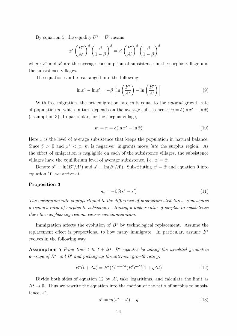
Immigration affects the evolution of B∗ by technological replacement. Assume the

replacement effect is proportional to how many immigrate. In particular, assume B∗

evolves in the following way.

Assumption 5 From time t to t + ∆t, B∗ updates by taking the weighted geometric

average of B∗ and B′ and picking up the intrinsic growth rate g.

B∗(t+ ∆t) = B∗(t)1−m∆t(B′)m∆t(1 + g∆t) (12)

Divide both sides of equation 12 by A′, take logarithms, and calculate the limit as

∆t→ 0. Thus we rewrite the equation into the motion of the ratio of surplus to subsis-

tence, s∗.

s∗ = m(s∗ − s′) + g (13)

24

Substitute equation 11 into equation 13:

s∗ = −δβ(s∗ − s′)2 + g (14)

As the phase diagram of figure 16 shows, in the equilibrium, the negative quadratic

term −βδ(s∗ − s′)2 balances the growth rate g. Therefore,

Proposition 4 In the long run, even if B∗ has an intrinsic tendency to grow at the

constant rate g, the surplus village’s ratio of surplus to subsistence, s∗ = ln(B∗/A∗) will

stabilize at

s′ +

√g

δβ

Figure 16: The phase diagram of s∗, the surplus-subsistence ratio of the sink area

Proposition 4 establishes the dominance of group selection over the growth advantage

of surplus. The growth advantage of surplus g contributes to the level but not the growth

rate of utility. The equilibrium utility of the surplus village increases with g but decreases

with δ: selection will be stronger when migration is more responsive.

3.7.2 A two-region model

The sea-of-village model solves the “partial equilibrium”: it describes the dynamics of a

single region but we are also curious about the “general equilibrium”. This section shows

how the global average surplus evolves in a two-region world.

The following two-region model inherits all the previous assumptions except the num-

ber of regions. Suppose region 1 and region 2 start identical; the baseline model specifies

everything inside each. Assume that their subsistence technologies, A1 and A2, grow at

the same constant rate gA and their surplus technologies, B1 and B2, grow at a variable

rate. In particular, if unconstrained by selection, B1 and B2 have an intrinsic tendency

to evolve as follows:

d lnBi = (gA + g)dt+ σdzi (15)

25

Here, g measures the growth advantage of surplus over subsistence. When g > 0, surplus

tends to grow faster than subsistence. The error terms zi’s (i = 1, 2) are independent

Brownian motions, Var(σdz) = σ2dt and z1 and z2 are independent with each other. I

introduce the stochastic growth of technology as the source of inter-regional variation in

the ratio of surplus to subsistence. The variation is the basis of group selection.

In the real world, both surplus and subsistence technologies, B and A, are subject

to drifts with random errors. But I fix the growth paths of A1 and A2 to keep the

levels of population equal between the regions. The equality of population simplifies the

calculation of the number of migrants and makes the model tractable. Now the inter-

regional variation comes from the randomness of the surplus growth only. The source of

the variation is not crucial to my result, for selection works on the difference of production

structures and the Brownian motion in the surplus growth has fully captured the variation

in the surplus-subsistence ratio.

Denote si ≡ ln(Bi/Ai), which measures the ratio of surplus to subsistence. Equa-

tion 15 implies the motion of si,

dsi = gdt+ σdzi (16)

Now assume that

Assumption 6

g > 0

If there were no migration, surplus sector would grow faster than subsistence sector.

The assumption allows both regions, if isolated, to grow steadily in living standards.

The question is under what condition group selection will suppress the trend of growth

when migration is allowed.

Group selection offsets the trend of growth by adding a “drag” term to the motion of

si. The drag arises when s1 6= s2. Following a similar derivation as we did for equation 14,

we can calculate the drag term as a quadratic of the difference between s1 and s2:

dsi = [g − I{si>sj}βδ(si − sj)2]dt+ σdzi

Here I{si>sj} is the indicator function that equals 1 if si > sj and 0 if otherwise. The

selection drag is conditional on the comparison of s1 and s2: if s1 > s2, region 1 is

relatively the surplus region. It attracts immigration from region 2, which drags s1 closer

to s2; if s1 < s2, region 1 is relatively the subsistence region. It receives no migration and

s1 will not be affected.

Since utility depends on the ratio of surplus to subsistence and we are interested in

the global average utility, the most interesting variables are the global average of si’s,

26

µ = 12(s1 + s2) and the inter-regional variation ν = 1

2(s1 − s2)2.13 The way µ evolves

describes the dynamics of the global living standards.

Applying Ito’s lemma, we can solve for the motion of µ and ν.

dµ = (g − βδν)dt+

√2

2σdz (17)

dν = (σ2 − 2√

2βδν32 )dt+ 2

√νσdz (18)

where z is a Brownian motion.

Ignoring the stochastic part, figure 17 graphs the phase diagrams of µ and ν. There

are two different scenarios. Which scenario arises depends on the relative positions of the

two nullclines, i.e. the curves of µ = 0 or ν = 0.

µ = 0 : ν =g

βδ(19)

ν = 0 : ν =1

2

(σ2

βδ

) 23

(20)

Comparing the relative positions of the nullclines solves the threshold condition for

the dominance of selection.

Proposition 5 If the growth advantage of surplus, g is larger than a threshold, e.g.

g >1

2(βδ)

13 (σ2)

23 (21)

µ will be rising: the growth advantage of surplus outpaces the force of selection. If g is

smaller than the threshold, µ will be declining: selection dominates the growth advantage

of surplus.

The possible decline of µ seems to contradict the constancy of living standards. To

address the problem, we can either set a lower bound of average surplus or specify that

the surplus growth rate increases with the relative rarity of surplus. Such modifications

appear ad hoc, but the ad hocery does not hurt my theory. First, these modifications are

reasonable features of reality; second, the theory is never meant to explain why living

standards had not been declining. The only thing that I need to show is the possibility

that selection can dominate the growth advantage of surplus. My model has derived the

condition when that happens.

The threshold in proposition 5 depends on σ2 because selection works on variation. If

surplus growth did not vary around the trend, surplus technology would grow at the same

rate in both regions and group selection would not take place between them. Increasing σ2

strengthens selection: it then requires a larger growth advantage of surplus to overcome

group selection.

13ν is equivalent to the sample variance: ν = 12 (s1 − s2)2 = [s1 − 1

2 (s1 + s2)]2 + [s2 − 12 (s1 + s2)]2

27

Figure 17: The phase diagrams of µ and ν

At a first look, selection appears weak. If β = 0.5, δ = 0.1 and σ = 0.02, the threshold

g is merely 0.1%, that is, living standards will be growing as long as surplus intrinsically

grows faster than subsistence by more than 0.1% per year. In the ancient times, global

population increased at about 0.1% per year. Therefore subsistence must have grown at

about 0.1%. It suggests, when gB < gA + g = 0.1% + 0.1% = 0.2%, living standards

cannot grow. In other words, group selection dominates the trend of growth even if

the intrinsic growth rate of surplus is twice as large as that of subsistence. Selection is

stronger than it appears.

However there is a serious limitation to the model. The model assumes a strong form of

selection: the immigrants’ technologies replace the natives’ technologies, no matter whose

methods of production are more efficient. The assumption is reasonable in the context of

wars but not in the other contexts. If people can choose what kind of technology to adopt

and if they always take up the more advanced technology when faced with a choice, will

group selection still dominate the growth advantage of surplus? The answer is yes. The

following simulations address the concern.

4 Simulation

4.1 Simulating group selection

The above models show how selection suppresses the growth of surplus. There are two

limitations. First, the sea-of-village model abstracts from the geographical feature of

28

the real world. Second, the models assume the immigrations’ technologies to replace

the natives’ technologies even if the latter might be more advanced. To address the two

concerns, I turn to computer simulation to study how strong and robust group selection

is indeed.

The strength of selection is of central interest because for my theory to be established,

selection must overcome a number of noises. Trade, cross-border learning, seasonal mi-

gration and distribution of books provide alternative ways for an idea to spread, ways

that are neutral to the surplus character of the idea. Group selection must overcome these

noises to suppress the growth of surplus. Empirically estimating these factors is difficult.

But if I can demonstrate the strength of group selection, that selection can dominate a

large advantage of surplus growth - hence the noises are relatively minor compared with

selection - then my theory should deserve more confidence.

To conduct the simulation, imagine a chess-board-like world divided into l × w grids

(figure 18). Each grid has the same production and utility functions and the same popu-

lation dynamics, as the baseline model specifies. Time is discrete. At period t, the state

of a grid economy (i, j) is {Aijt, Bijt, Hijt}, i.e. the subsistence technology, the surplus

technology and the level of population.

Figure 18: The chess-board world of 5× 5 grids

For grid (i, j), assume its levels of technology, Aij and Bij, evolve this way:

Aij(t+ 1) = Aij(t)(1 + gAij + σAεAij) + selection effect (22)

Bij(t+ 1) = Bij(t)(1 + gBij + σBεBij) + selection effect (23)

The error terms εA and εB both follow a normal distribution, εA, εB ∼ N(0, 1), i.i.d.

To prevent a downward trend of living standards when group selection dominates, assume

that gB rises with the relative rarity of surplus. In particular,

gBij = gB

[1 +

(Bij

Aij

)α](24)

To minimize the effect of the endogeneity of gBij, I set the parameter α = −10 so that the

adjustment term is negligible when Bij/Aij > 1. The endogeneity of gBij does not weaken

29

the robustness of my simulation because the adjustment raises the growth advantage of

surplus and thus is unfavorable to my hypothesis of surplus suppression.

I fix gAij across all grids: gAij = gA. The parameters gA, gB, σA, σB are set ex-

ogenously. In the baseline simulation, I set gB > gA: surplus intrinsically grows faster

than subsistence. I also assume σ ≡ σA = σB. I will show how the strength of selection

increases with σ.

In each period, people decide whether they should move to one of the neighboring

grids for higher living standards. For any pair of bordered grids, if grid 1 has a higher

utility than grid 2, some of the residents of grid 2 will move to grid 1. Assume the

migration rate to be equal to

Migrants

Population of grid 2= θ(lnU1 − lnU2) (25)

Equation 25 sets a different rule for migration than the theoretical model does. The

theoretical model rules out the difference of utility across regions by assuming instant

free migration. But equation 25 introduces θ, the measure of how responsive migration

is to the difference of utility. When θ → ∞, the simulated migration works in the same

way as in the theoretical model. Setting a finite θ makes the simulation closer to reality.

It also allows me to evaluate the variance of utility levels across different regions.

Migrants spread knowledge from hometowns to destinations. I simulate two different

scenarios, each assuming a different way of knowledge spread.

The first scenario is called “pure replacement”. It is the same mechanism the theoret-

ical model has adopted: the immigrants’ technologies replace the natives’ technologies.

The second scenario is called “combining the best”. People are allowed to choose what

technologies to adopt. If the immigrants bring a more advanced technology, the natives

will update their own in the same way as “pure replacement”; but if the immigrants’

technologies are inferior to the natives’, the natives will keep their old technologies, and

the immigrants will convert to the natives’ technologies as well.

Combining the best favors the spread of subsistence as pure replacement does. For two

regions that start identical, if one of them improves subsistence productivity, population

growth will lower its living standards, and people will emigrate to spread the improved

subsistence technology. However, if it is surplus productivity that improves, no emigration

will occur and the surplus technology has to remain local.

Overall, selection is weaker under combining the best than under pure replacement.

Pure replacement not only spreads subsistence but also degrades surplus. In contrast,

combining the best only spreads subsistence but never degrades surplus. The reality is

somewhere in between.

I simulate both scenarios. In my baseline simulation, I parameterize gA = 1%, gB =

0.5% and σA = σB = 5%. The other parameters are set to make a period roughly

30

equivalent to a decade.14

Including pure replacement and combining the best, I compare four different scenarios

in total (figure 19). The other two scenarios are purely Malthusian - they rule out group

selection. The first one forbids migration and the second one forbids the natives to learn

from the immigrants. After 1, 000 decades, the global average utility grows from 1.5 to 12

under both Malthusian scenarios: solely the Malthusian force fails to check the growth.

In contrast, group selection preserves the constancy of living standards: under either pure

replacement or combining the best, the average utility never exceeds twice the original

level throughout the simulated history that spans 10, 000 years.

Figure 19: The evolution of utility under different assumptions

The stability of living standards does not mean technology is stagnant. In fact, group

selection accelerates technological progress. Population grows faster under the selection

scenarios than under the Malthusian scenarios (figure 20).

Within each grid, the dynamics of utility are more volatile than the global average.

Figure 21 illustrates three particular regions: one in the corner, another on the side and

the other in the center. Despite the wild fluctuations of utility - with cycles that span

thousands of years - there is no trend of growth in any of the three regions.

14Appendix B table 9 lists the parameterizations for the baseline simulation.

31

Figure 20: The population growth under different assumptions (log)

Figure 21: The evolution of regional utility

32

4.2 Robustness

To check the robustness, I vary parameterization and observe when the constancy breaks.

There are two sets of parameters playing the key role: the growth advantage of surplus

(gB − gA) and the variation of the error terms (σA and σB).

I fix gA at 0.5%. Then I vary gB from 0% to 2%, and σ ≡ σA = σB from 0% to 15%.

For each pair of parameters gB and σ, I run a simulation that spans 600 decades on a

10 × 10 grid world. If the global average utility rises more than 25% between the 300th

decade and the 600th decade, I mark a triangle on figure 22; otherwise, I mark a circle.

Figure 22: Robustness check

Figure 22 shows the results. Growth is less likely to appear with a larger standard

deviation of the error terms. It confirms the finding in the theoretical model: the strength

of selection increases with variation. With enough variation, group selection can dominate

a significant growth advantage of surplus. For example, under pure replacement, when

σ = 5%, utility grows less than 25% over 3, 000 years when gB = 1.4% and gA = 0.5%.

Group selection is indeed a strong force.

As figure 22 shows, the area of growth (triangle) is larger under combining the best

than under pure replacement: selection is weaker under combining the best. But the

simulation has underestimated the strength of selection in this scenario. Here growth

is more likely to appear because sooner or later, some grids will emerge strong in both

surplus and subsistence; their neighbors are left so far behind that the immigration can

no longer affect the technologies of these grids. The living standards of these grids will

then grow steadily by the growth advantage of surplus.

In the real world, such groups do not last long. First, they trigger wars and invasions,

33

i.e. pure replacement. Second, even if there is no invasion from the outside, population

growth will split such a group into more groups, which border each other, share similar

technologies and thus compete with each other on an equal level. Selection among the

split groups will constrain the growth of living standards.

4.3 A duet dance between surplus and subsistence

The constancy of living standards requires surplus to grow at the same rate as subsistence

in the long run. But the mere equality of long-run average growth rates is not enough.

World population growth had accelerated for several times, which implies that subsistence

growth also occasionally accelerated (figure 23). Can surplus growth catch up at each

time when subsistence growth accelerates?

Figure 23: The historical world population, from 10000 BC to 1800 AD

Figure 24: The duet dance between surplus and subsistence

34

The answer is yes. Surplus growth closely matches subsistence growth like a duet

dance. I simulate a history of 2, 000 decades for a world of 10 by 10 grids. I fix gB at

1% throughout; but I make gA jump from 0.25% to 0.75% in the middle at the 1001st

decade. So there appears a kink in the middle of the path of global average subsistence

technology (figure 24).

Now I conduct a Chow test to check whether the path of surplus growth shows a kink

at the same date:

∆ log(Surplus) = 5e−3

(1e−3)+ 10e−3

(0.6e−3)× break dummy + ε

The test yields a p-value as low as 10−6, rejecting the null hypothesis of no kink. Notice

that the estimated coefficient of the break dummy, 10e−3 is exactly twice as large as

the constant term, 5e−3. It means that when the growth rate of subsistence triples, the

growth rate of surplus triples too. Though gB is fixed, surplus growth catches up with

subsistence growth fast and fully.

5 Evidence

Empirically, it takes three historical facts to establish my theory. I shall show that the

division of surplus and subsistence was a salient feature in the real world, that source-sink

migration existed in history and that migration and wars had hindered surplus growth.

5.1 The empirical division of surplus and subsistence

To establish the first fact, I turn to the English price series collected by Gregory Clark

(2004). I use the “affordability” of different goods to explain the birth and death rates

between 1539 and 1800.15

I calculate the indices of “arable wage” and “pasture wage” for the measure of af-

fordability. The arable wage, for example, is the logarithm of the ratio of the nominal

average income to the price index of arable goods.16 It measures the maximum amount

of arable goods that an average person could buy with all her income.

I regress the annual birth and death rates on the wage indices and other controls.17

In case an ordinary least square regression give biased estimates of the standard errors,

I use the Newey-West method for the consistent estimation of the standard errors.

15Wrigley and Schofield (1981) estimated the annual numbers of baptisms and burials in England. The

series is the most commonly used in the modern literature on English demography.16Arables include wheat, rye, barley, oats, peas, beans, potatoes, hops, straw, mustard seed and saffron.

Pastures include meat, dairy, wool and hay, of which meat includes beef, mutton, pork, bacon, tallow and

eggs. Clark (2004) compiled the annual price series for most of the products. He also derived aggregate

price indices of arables and pastures.17I control for the climate with data from Booty Meteorological Information.

35

With the guide of the Akaike information criterion, I choose to run the regressions

up to four years’ lags. But I only report the cumulative dynamic multipliers up to two

years’ lags. The coefficients sum up the effects of the impact year and the last two years

ahead.

I cannot reject the hypothesis that both the birth and death rates and the wage indices

have unit roots; but I can reject the hypothesis that their first-order differences have unit

roots. Therefore, I regress the difference of the birth and death rates on the difference of

the wage indices. If there are K wage indices up to lag l, I estimate an equation adapted

from the following one:

∆Yt = β0 +K∑i=1

l+1∑s=1

βis∆Xit−s+1 + Controls + µt (26)

I adapt the above equation into equation 27 to estimate the cumulative dynamic

multipliers and their standard errors.

∆Yt = δ0 +K∑i=1

(l∑

s=1

δis∆2X i

t−s+1 + δi l+1∆X it−l

)+ Controls + µt (27)

Here the coefficients δ’s are the cumulative dynamic multipliers: δis =∑s

j=1 βij.

I conduct three experiments with six pairs of regressions (table 1 and table 2).

In the first experiment, I compare the effects of the arable wage and the pasture wage

(columns B(1) and D(1)). The arable wage has significant effects on both the birth

rate and the death rate. Doubling the arable wage would raise the birth rate by 1.14

percentage points and lower the death rate by 1.11 percentage points within three years.

In contrast, the pasture wage has no significant effect on either rate. The difference of

effects is not caused by the difference of sectoral size - the size of the pastures as a share

of economy was about 3/4 that of the arables. Rather, it is evidence that the arables are

a relative subsistence to the pastures.

The second experiment (columns B(2) and D(2)) shows that within the category of

arable goods, barley and oats are a relative subsistence to wheat. In pre-modern England,

wheat had been a more expensive source of calorie than barley and oats. The rich had

wheat bread while the poor ate porridges. Though barley and oats combined were smaller

than wheat as a share of economy, the barley and oats wage has a much larger impact

on the birth rate and the death rate.

In fact, as the third experiment shows, the barley and oats wage explains most of

the demographic effect of the average income. Compare B(3) with B(4) and D(3) with

D(4). Adding the barley and oats wage as a regressor takes away the explanatory power

of the real income. But adding the pasture wage has no effect at all - columns B(6)

and D(6) report the placebo test. Accounting for merely a 10% share of the English

economy, barley and oats exerted a demographic impact far beyond proportion. The

36

Table 1: What affects the birth rate?

Dependent Variables ∆ Birth rate (%) (the mean birth rate=3.31%)

B(1) B(2) B(3) B(4) B(5) B(6)

∆ Arable wage1.14***

(0.23)

∆ Wheat wage0.07

(0.20)

∆ Barley and Oats wage1.03*** 0.83*** 0.72**

(0.32) (0.29) (0.28)

∆ Pasture wage0.84 0.76 0.70

(0.86) (0.80) (0.77)

∆ Clark real earning2.17*** 0.65 2.08***

(0.53) (0.59) (0.47)

∆ Wrigley real wage0.07

(0.41)

R2 0.24 0.25 0.20 0.23 0.33 0.25

Observations 262 262 262 262 257 262

Notes: All the coefficients are the sum of the first three years’ effects. The models

control for the linear, quadratic and cubic trends and include the climate and plague

dummies up to two years’ lags. Merely regressing the birth rate on the controls has

R2 = 0.06, and regressing the death rate on the controls has R2 = 0.23. *,** and ***

denote significance at the 90%, 95% and 99% levels respectively.

37

Table 2: What affects the death rate?

Dependent Variables ∆ Death rate (%) (the mean death rate=2.75%)

D(1) D(2) D(3) D(4) D(5) D(6)

∆ Arable wage-1.11**

(0.43)

∆ Wheat wage-0.11

(0.33)

∆ Barley and Oats wage-0.96 -0.93 -0.91

(0.60) (0.62) (0.63)

∆ Pasture wage1.06 1.32 0.99

(1.06) (1.09) (1.01)

∆ Clark real earning-1.65** -0.10 -1.81**

(0.73) (1.01) (0.85)

∆ Wrigley real wage-0.33

(0.85)

R2 0.31 0.32 0.26 0.29 0.35 0.29

Observations 262 262 262 262 257 262

Table 3: The comparison of different methods of regression

Dependent variable: birth rate

Difference Level

OLS SUR NW NW

Arable wage1.15*** 1.15*** 1.15*** 0.54***

(0.3) (0.28) (0.23) (0.12)

Pasture wage0.84 0.84 0.84 -0.09

(0.57) (0.53) (0.86) (0.3)

R2 0.24 0.24 0.24 0.66

Notes: “Difference” means regressing the difference of the birth rate on the differ-

ences of the explanatory variables. “Level” means regressing the level of the birth

rate on the levels of the explanatory variables. OLS, SUR and NW are abbrevia-

tions for ordinary least square, seemingly unrelated regression and Newey-West.

38

pattern is robust if I replace Clark’s series of real earning with Wrigley’s series of real

wage (columns B(5) and D(5)).

In Appendix B, table 5 and table 6 report the seemingly unrelated regressions (SUR)

that take into account the correlation of the error terms. Table 7 and table 8 report the

“level regressions” that do not take differences. I compare the different methods using the

regression of birth rate on arable wage and pasture wage as an example (table 3). OLS,

SUR and NW yield similar estimates under the regression of difference on difference. In

comparison, regressing level on level underestimates the difference of demographic effect

between surplus and subsistence. What is common among all these regressions is the

significance pattern: the arable wage significantly contributes to the birth rate but the

pasture wage does not.

5.2 The magnitude of source-sink migration

The empirical division of surplus and subsistence provides basis for the source-sink migra-

tion. Across different areas, equilibrium living standards vary as production structures

differ. Therefore the source-sink migration emerges.

The source-sink pattern is best documented in the context of rural-urban migration.18

Since John Graunt’s (1662) pioneering work, researchers have been fascinated by the

phenomenon of urban natural decrease. The death rate was higher than the birth rate in

the urban areas in pre-modern Europe; and the urban natural decrease often coincided

with the rural natural increase. Thus the rural area played the role of demographic source

and the urban area played the role of demographic sink.

Jan de Vries (1984) summarized the previous studies and decomposed the net change

of urban population into net immigration and the natural change.19 As figure 25 shows,

during most of the time between 1500 and 1800, urban population had been growing in

both Northern and Mediterranean Europe. However, despite the net increase, the urban

population had been declining “naturally” - the death rate was higher than the birth rate

in the cities. Take the period 1600−1650 for example. During that half century, Northern

Europe witnessed an annual growth of 0.32% in its urban population; but meanwhile,

the urban death rate exceeded the birth rate by 0.33%. So it took a flow of annual

rural migrants that amounted to 0.65% of the size of the urban population to achieve the

observed urban growth.

The pattern of migration exposes another weakness of Malthusianism. Between 1800

and 1850, there was a spike in the growth of urban population in Northern Europe. The

18Certainly, source-sink migration is not limited to the rural-urban context, neither is rural-urban

migration the most important channel for group selection to take effect. I use the rural-urban migration

as evidence that difference of production structures causes source-sink migration.19“The European Urbanization, 1500-1700”, p. 203 and p.208.

39

Figure 25: The source-sink migration in pre-modern Europe (De Vries, 1984)

spike suggests a rise in the urban living standards. According to the classical theory,

improvement in living standards would cause a faster natural growth of the urban popu-

lation. But in fact, the half century of 1800-1850 witnessed a widened gap between urban

death rate and urban birth rate.

Malthusian theory cannot account for the contradiction, but my theory can explain it

easily. In the years after 1800, manufacturing and commerce grew fast in the urban areas;

and agriculture grew fast in the rural areas. The rural-urban difference of production

structure was widened, so that the urban lifestyle attracted more immigrants than in the

centuries before. The flood of immigrants lowered the average subsistence by so much

that the natural growth rate of the urban population decreased further. As proposition 3

states, the depth of the demographic sink increases with the difference of production

structures.

5.3 Selection against surplus boom

The previous section establishes the historical relevance of source-sink migration. The

source-sink pattern makes it possible for group selection to suppress surplus growth. Since

surplus promotes individual fitness at the expense of group fitness, it is tautological to say

that group selection hinders surplus growth. What matters is the strength of selection,

i.e. the frequency and intensity of group competition.

Fatal clashes between groups are a perpetual human condition. Of the fourteen groups

studied in Mae Enga - a modern hunter-gatherer society in Papua New Guinea, five went

40

extinct in tribal clashes over a 50-year period (table 4).20 The extinction rate suggests a

harsh selection against surplus cultures and technologies.

Table 4: Group extinctions in Papua New Guinea and Irian Jaya

Region Groups Extinctions Year Extinction rate per century

Mae Enga 14 5 50 59%

Maring 32 1− 3 50 6− 18%

Mendi 9 3 50 56%

Fore/Usufura 8− 24 1 10 35− 74%

Tor 26 4 40 34%

Source: Soltis et al. (1995), table 1.

Heralding the end of the hunter-gatherer epoch, the agricultural revolution demon-

strated the strength of group selection. Despite its negative effect on living standards,

agriculture encroached on the hunter-gatherer territory as a subsistence technology.

After the agricultural revolution, the world was divided into the nomadic zones and

the arable zones. Clashes between them disrupted economic growth over and over again.

Around 1000 BC, the nomads from the hinterland of Europe destroyed a number of highly

developed kingdoms in Levant and Anatolia. The Hittites, the Minoans, the Mycenaeans

lost the complex social order they had built. Urban centers, artistic representation, elabo-

rate writing system, large-scale trading, shipping and construction vanished; civilizations

were reduced to impoverished, illiterate, technically backward and more violent small

communities. Underlying the economic decline is the pattern of source-sink migration -

“the invasions were not merely military operations, but involved the movements of large

populations, by land and sea, seeking new lands to settle” (Bryce, 1998).

Similar catastrophes came upon humanity frequently. The fall of western Rome under

the Visigoth and Hunnish intrusion, the overwhelming victory of the barbarian Jin over

the civilized Liao empire, the Mongol destruction of Baghdad - the “center of learning”

and then the largest city of the world - all exemplify the intense group selection that

suppresses surplus economies.

Moreover, people respond to selection by intentionally cutting down surplus for group

survival. For example, the warring period of China (476 BC - 221 BC) witnessed a series

of reforms in different kingdoms.21 In response to the constant nomadic harassment,

King WuLing of Zhao (340 BC - 295 BC) commanded his subordinates to take off the

conspicuous dress of wide sleeves and long robes and switch to the nomadic uniform

20In place of the extinct groups, new groups form out of the old groups that survive and expand.21To name a few, Li Hui conducted a reform in Wei, Wu Qi in Chu, Shen Buhai in Han, Shang Yang

in Qin and King Wuling in Zhao.

41

- pants, belts and boots - so that they could fight as cavalry. Acclaimed as China’s

Peter the Great, King Wuling transformed Zhao into a serious rival against Qin, then the

strongest kingdom.

Half a century before Zhao’s reform, Qin rose to dominance by Shang Yang ’s reforms

in 356 BC and 350 BC. The reformer punished merchants, rewarded peasants, forbid

migration, restricted entertainment and adopted censorship - in a word, he cut down sur-

plus and promoted subsistence. The living standards declined so much that the ordinary

people would flee the kingdom whenever they could evade the severe punishment of law.

But the kingdom stood out to be the strongest. It defeated all the rivals and united

China in the following one and a half centuries.

A contemporary philosopher, Xun Zi (313 BC - 238 BC) compared the military system

of Qin with that of the other kingdoms, saying, “Qin is different from all the others. The

people are poor and the government is cruel. Whoever hopes for a better life can do

nothing but combat hard. This makes Qin army the strongest of all.”22

Qin’s ideas of governance had a lasting impact on the later Chinese dynasties. They

were in sharp contradiction with Adam Smith’s economic views. The predecessors of

Adam Smith valued agriculture more than commerce, and restricted trade and private

property, not because they failed to appreciate market economy, light tax and division

of labor, but because their goal was not the individual’s welfare but the group’s survival

and expansion.

Adam Smith is unique not because he had a new theory that no one had raised before,

but because he lived on the eve of the modern era, when individual welfare is reconciled

with group survival and expansion. He prophesied the day at dawn.

6 Discussions

6.1 Smithian policies in Malthusian era

Published in 1776, The Wealth of Nations heralded the breaking of the humdrum Malthu-

sian constancy. Some believe Adam Smith to be slightly ahead of his time. They doubt

the Smithian policies could ever affect the equilibrium living standards before 1800. In

A Farewell to Alms, Gregory Clark said “[I]n 1776, when the Malthusian economy still

governed human welfare in England, the calls of Adam Smith for restraint in government

taxation and unproductive expenditure were largely pointless. ... [while] those scourges

of failed modern states - war, violence, disorder, harvest failures, collapsed public infras-

tructures, bad sanitation - were the friends of mankind before 1800.”

But my thesis is that Smithian policies can improve living standards, not only in

22An excerpt from Xun Zi, chapter Yi Bing (On Wars).

42

the short run but also in the long run, not only in Solow’s time but also in Smith’s

time. Adam Smith advocated laissez-faire, light tax and division of labor. Applying

these ideas to economic policies will raise productivity of all sectors, but manufacturing

and commerce benefit more from them than agriculture does. As the ratio of surplus

to subsistence increases, the economy enjoys a higher equilibrium living standard. This

explains the prosperity of ancient market economies, such as Roman empire and Song

dynasty.

As of the “friends of mankind” - wars, violence, disorder and collapsed public in-

frastructures, if they destroy more surplus than subsistence, they may cause the living

standards to decline to a lower equilibrium in the long run. This might be the reason why

it took more than a thousand years for Europe to economically recover from the collapse

of Western Roman Empire.

6.2 Why farm?

The two-sector model also explains why peasants were worse off than their hunter-gatherer

ancestors after the agricultural revolution. People had less leisure, worse nutrition and

larger inequality after they took up agriculture. In light of my theory, agriculture plays the

role of a subsistence technology. By tilting the production structure towards subsistence,

it caused the living standards to decline. But here follows another puzzle:

“Why [should people ever] farm? Why [did they] give up the 20-hour-work

week and the fun of hunting in order to toil in the sun? Why work harder,

for food less nutritious and a supply more capricious? Why invite famine,

plague, pestilence and crowded living conditions?” (Harlan, 1992)

Group selection addresses the second puzzle. Although hunter-gatherers enjoyed a

better life, they achieved their welfare by living a relatively surplus-rich lifestyle at the

expense of group fitness. When agriculture appears, the surplus-rich hunter-gatherer

societies cannot compete with the groups that have switched to agriculture. The bi-

ased migration from the agricultural areas to the hunter-gatherer areas completed the

transition.

6.3 Surplus explosion and the industrial revolution

How did the mankind finally break the shackle of group selection? How did the industrial

revolution happen? My theory provides a new perspective. In the other chapters of my

dissertation, I will work out a theory of surplus explosion as a natural extension of the

paper.23 Here let me sketch the idea briefly.

23The other two chapters are “Institutional Selection: A New Unified Growth Theory of Malthusian

Stagnation, Industrial Revolution and Modern Economic Growth” and “Horse, Agriculture, Islam and

43

Group selection constrains surplus and spreads subsistence. A commodity or behavior

can burst into wide adoption when it switches from surplus into subsistence. I call such

transitions a surplus explosion. For example, agriculture first arose for the production

of status goods (Mithen, 2007) - the tribal elites cultivated “crops” for festivals and

ceremonies. Such agricultural practice was less efficient than hunting and gathering in

producing calorie - it was a local surplus activity. Over time, domestication raised the

calorie productivity of the “status crops”, which finally exceeded that of hunting and

gathering. Thus agriculture switched into subsistence. It won over the force of group

selection to spread to the rest of the world.

Around 3500 BC, another surplus explosion took place on the Caucasian steppe where

horses were domesticated into a tool of war. The people that first domesticated horses

spread fast by military conquests. Caucasia became the origin of Indo-European language

family.

Likewise, Alexander the great spread hellenism by march and conquest. His army

inherited military techniques from the constant wars between Greek city states in the

older generations. The war skills turned from surplus into subsistence as Macedon united

Greece.

The industrial revolution follows the same pattern but with a different kind of surplus.

Following the spirit of Becker in a series of his work on the quality and quantity of children,

the literature of Unified Growth Theory has identified the quality of children - human

capital - as the pivot of transition.24 Either by genetic drift or population growth, what

used to be surplus - human capital - turned into subsistence. Human capital helped a

state develop science, defend territory and send out colonists.

Surplus explosions have happened many times before, in various forms. Among them,

the industrial revolution is unique by its content of surplus. The usual surpluses, dia-

monds and yachts cannot switch into subsistence; weapons switch but it does not improve

living standards. Human capital in scientific knowledge is different. With a persistent ef-

fect on economic growth, it strengthens the countries rich in it and brings about universal

welfare and steady progress.

6.4 The Evolutionary Biology of Economic Welfare

My theory implies that economic welfare is an evolutionary biological phenomenon. Wel-

fare improvement relies on surplus growth. Surplus growth is rooted in the conflict of

reproductive interest between individual and group. The same conflict gives rise to sur-

plus traits in plants and animals, the traits that help the individuals compete with the

others, but divert resources from supporting a denser population.

Science: Surplus Explosions in Human History.”24Galor and Moav (2002), Galor (2002), Clark (2007) and Galor (2011)

44

For example, peacocks bear the extravagant tails to signal their physical health to

peahens. The tail makes a credible signal because it is a handicap that exposes the

owner to a higher risk from predators. The density of peacocks would be larger if they

collectively refrained from the signaling game.

The animals’ conspicuous traits are constrained by group selection too. Guppy is

a popular aquarium fish species. Wild-type male guppies have colorful splashes, spots

and stripes on their bodies to attract females. Researchers moving the fish from a high-

predator environment to a low-predator one found that the male guppies become brighter

in color - the pressure on surplus is loosened when group competition is less intense.25

Personally, I realized the biological analogy at a trip to Muir Woods, a forest 19

kilometers north of San Francisco that features coastal redwoods. The redwoods can

grow up to 100 meters high, as they compete intensely with each other for sunshine. The

height serves the need of the individual trees but it diverts nutrition which could support

a denser forest. Pursuing the individual fitness hurts the group fitness.

The height of redwoods, the tails of peacocks, the colors of male guppy and the surplus

of human society all are governed by the same principle of evolutionary biology: conflict

is universal between group and individual, hence surplus is prevalent in nature. Surplus

tends to escalate under the force of individual competition, but group selection harshly

suppresses it.

Economists have understood “conspicuous consumption” for a long time. Thorstein

Veblen coined the phrase to describe how unproductive retinue and long skirts are used

to show off one’s wealth, to the effect of attracting mates. Spence (1973) gave the idea a

signaling model. Biologists use the same model to study conspicuous traits in the context

of sexual competition - in biology, surplus is mostly about sex. But in the real world, we

rarely associate our passion for art and status with sexual purposes; we do not intend to

impress the others as often as we consume surpluses. How can sex explain most of the

surplus?

In fact, sexual competition has a larger scope than signaling games. Complementary

to signaling, there is another mechanism of sexual competition that magnifies the con-

spicuous traits far beyond the level a signaling model would predict. That mechanism

is called “Fisherian runaway”, first proposed by biologist Ronald Fisher (1915). Under

runaway mechanism, a conspicuous trait that is first caused by signaling can run out of

control by a positive feedback “runaway” mechanism.

For example, suppose signaling produces a costly male trait - music playing - and

a female preference for the trait. At the signaling stage, females value music talents

because they reveal one’s sense of pitch, which makes a man more effective at hunting.

But now, the fact that the other females like the trait gives a female an extra reason to

25The Guppy Project of University of California, Riverside.

45

choose a musically talented man: he can pass on his genes of music talents to her son,

who in turn will be attractive to the females of the next generation. So the male trait

and the female preference coevolve to be strengthened; men become showier and showier

and women choosier and choosier. Since the mating choice is two-way between male and

female, females develop no less music talents than males; and males are as choosy as

females about the music talents in their partners. At last, runaway mechanism produces

talents as great as Lloyd Webber and Sarah Brightman.

Altogether, the positive feedback magnifies the conspicuous traits. Our talents of

music are far beyond the explanation of mere signaling. Yet the origin of the traits is

still within the domain of sexual competition - Fisherian runaway is a type of sexual

competition. The existence of the mechanism suggests, the conflict between group and

individual is much more intense than we might think with the signaling view. The

distinction of surplus and subsistence is deeply rooted in evolutionary biology.

6.5 Methodology

A believer in Milton Friedman’s methodology (Friedman 1953) might reject my theory.

Why challenge a theory that has made the right prediction? Why does it matter that

Malthus assumed away the conflict of interest between individual and group? Didn’t

Friedman say, the more unrealistic the assumption is, the better the theory?

Friedman was wrong. We accept unrealistic assumptions, except if the theory would

predict awry when we make the assumptions realistic. In other words, the unrealistic

assumptions cannot be crucial ones on which the prediction relies. Friedman himself

was using this extra condition to attack the traditional view of Phillips curve. When he

introduced inflation expectation, stagflation had not happened, yet Friedman figured out

the mistake in the conventional wisdom because he found the traditional theory sensitive

to the introduction of expectation, which was merely a more realistic assumption.

As Solow (1956) put it, “All theory depends on assumptions which are not quite true.

That is what makes it theory. The art of successful theorizing is to make the inevitable

simplifying assumptions in such a way that the final results are not very sensitive. A

‘crucial’ assumption is one on which the conclusions do depend sensitively, and it is

important that crucial assumptions be reasonably realistic. When the results of a theory

seem to flow specifically from a special crucial assumption, then if the assumption is

dubious, the results are suspect.”

This paper shows how crucial the one-sector assumption is to Malthusian theory.

Since the assumption is dubious, the classical theory is suspect.

46

7 Conclusion and Limitations

For more than two hundred years, scholars have taken for granted Malthus’s explanation

for the constancy of living standards. The conventional wisdom is wrong.

Different from the Malthusian version of history, this paper suggests the following

basic story. Imagine a world where people live on two things: grain and diamonds.

Population rises with grain production, therefore the average consumption of grain is fixed

in the long run. But population hardly responds to changes in diamond productivity. If

diamond productivity grows faster than grain productivity, people will live a better and

better life by having more and more diamonds each. Such had never happened until

1800. Throughout the thousands of years before that time, the diamond productivity

had grown at the same rate as the grain productivity.

The cause of the balanced growth is group selection. People organize themselves into

competing groups. When a group is relatively more productive in grain production, each

of its members will have fewer diamonds than their neighbors do. Greed drives them

to move abroad. As they move, they bring along the technology of their hometown and

spread it to the other places. The consequence is, grain technology spreads easily by

migration, but diamond technology is hard to disseminate. When the spread advantage

of grain offsets the growth advantage of diamonds, the growth of grain and diamonds are

balanced and the living standards are constant all over the world.

There are five major contributions the paper is meant to make.

• First and foremost, it shows that Malthusian theory cannot explain the constancy

of living standards. The paper provides a new explanation to replace it.

• Second, the two-sector framework explains why Malthusian theory is weak empir-

ically. The classical theory fails to capture the variation of birth and death rates

because it has missed two of the three factors that affect the long-run equilibrium.

• Third, the theory explains the puzzle of the agricultural revolution - why living

standards declined after the mankind took up agriculture and why agriculture dom-

inated the world despite its negative effect on living standards.

• Fourth, the paper shows how economic policies can improve long-run living stan-

dards even in the Malthusian epoch. What Adam Smith advocated - long-lasting

peace, light tax burden, property rights protection and laissez faire - raise living

standards by tilting the production structure. This explains the prosperity of the

ancient market economies, including the Roman and Song empires.

• Fifth, the theory reveals the hidden law of evolutionary biology in economic growth.

The Malthusian constancy, the industrial revolution and the burst of modern eco-

47

nomic growth can all be understood in an evolutionary biological framework, with

countless analogies in nature.

Altogether, this paper presents a multi-sector Malthusian framework, a source-sink

migration model, a theory of group selection and a sketch of the idea of surplus explosion.

These theories are not without limitations, but the limitations suggest future research

direction.

For example, I highlight the importance of migration at spreading subsistence ideas.

But there are many other ways for an idea to be spread - local learning, seasonal migration

and distribution of books. These channels do not favor either surplus or subsistence. It

is an empirical question whether migration is strong enough to dominate these noises.

In the paper, I turn to computer simulations to demonstrate the strength of selection;

yet the theory would be much strengthened if there were direct evidence on the relative

importance of migration.

Moreover, it is hard to categorize military strength to either surplus or subsistence.

Military strength is the best example of surplus explosions: it frequently switches between

surplus and subsistence. The flexibility makes it hard to interpret the early expansion of

Roman Empire. Rome built its military success on advanced weapons and organization

of troops, which resulted from its manufacturing advantage and sophistication of gover-

nance. This particular episode contradicts the law of surplus suppression. In another

dissertation chapter, I will develop a framework to understand “the third sector” - the

military sector of an economy.

Last but not the least, the theory is silent about internal disorder. Internal disorder is

no less important than external threat in the decline of civilizations. It is closely related

to social inequality, which I ruled out by assuming homogeneity of population. In my

future research, I shall put inequality back into my theory and study its interaction with

surplus growth. Surplus is meant for signaling one’s relative status - there would be no

need for surplus in a perfectly egalitarian society. In this sense, inequality breeds surplus

culture and thus contributes to long-run living standards. However, if inequality runs

out of control, social disorder and foreign invasion will fall upon the economy. Therefore

lasting economic progress cannot rely on the arms race of hedonism. This marks the

difference between the Roman prosperity and the modern economic growth. While the

Roman surplus were at the mercy of the political elites’ licentious spending, the modern

growth is bolstered by trade, science and good institutions - a comparison in the same

spirit as how the merchants’ cities outpaced the princes’ cities (Delong and Shleifer, 1993),

hence the theme of my next dissertation chapter, “Institutional Selection: A New Unified

Growth Theory of Malthusian Stagnation, Industrial Revolution and Modern Economic

Growth”.

48

Appendices

A Proofs

A.1 Proportionality between gA and gH

Proposition 6 If an isolated economy has constant growth rates of technology gA and

gB, then gA − (1− γ)gH converges to 0.

Population evolves in the following way:

gH = δ(lnx− ln x)

Since x = A(1− β)γHγ−1 (equation 2),

gH = δ[lnA+ γ ln(1− β) + (γ − 1) lnH − ln x]

Denote M ≡ lnA+ (γ − 1) lnH, then

gH = δ[M + γ ln(1− β)− ln x]

The motion of M follows

dM = gA + (γ − 1)gH

= gA + (γ − 1)δ[M + γ ln(1− β)− ln x]

Since (γ − 1)δ < 0, M will stabilize at

M∗ =gA

(1− γ)δ)− γ ln(1− β) + ln x

dM = gA − (1− γ)gH converges to 0.

A.2 Assumptions of the two-sector model

I make the following assumptions to prove the production structure theorems and “surplus

is free” theorems.

1. Conflict of interest: The utility function U(E) is not a transformation of the

growth rate of population n(E).

2. Homogeneity: People have the same preference.

3. Strict monotonicity: The utility function U(E) and the growth rate of population

n(E) are strictly increasing in consumption E.

49

4. Endowment economy: Assume an endowment economy where labor is not an

input. When the group size is H, the individual choice set is a 1H

fraction of the

aggregate set of production possibility.

5. Rank preservation: If a good is a relative surplus to another at a bundle of

consumption E, it is a relative surplus at all bundles of consumption.

6. Concavity and Continuity: The utility function is continuous, strictly concave

and continuously differentiable. The production possibility frontier is continuous

and strictly concave. The production function is the continuously differentiable.

A.3 Production structure theorem and surplus-is-free theorem

The production structure theorems state that:

1. For an economy on a stable equilibrium, a positive shock of surplus technology

always improves equilibrium living standards.

2. If the subsistence is not a Giffen good, an economy of a more surplus-oriented

production structure always has a higher equilibrium living standard, other things

being equal.

The “surplus is free” theorems state that:

1. For an economy on a stable equilibrium, a surplus culture always improves equilib-

rium living standards.

2. If the subsistence is not a Giffen good, an economy of a more surplus-oriented social

preference always has a higher equilibrium living standard, other things being equal.

Proof: As in figure 26A, draw a ray from the origin. Let the angle between the ray

and the horizontal axis be k ∈ [0, π/2]. The ray crosses the constant population curve at

E(k). Since preference is complete, there exists an indifference curve that passes through

E(k). Define u(k) as the absolute value of the slope of that indifference curve at point

E(k). u(k) varies as k changes.

Then shift the production possibility frontier in proportion to the place where it passes

through E(k). Define p(k) as the absolute value of the slope of the production possibility

frontier at point E(k). Since production possibility frontier is continuous and strictly

concave, p′(k) < 0.

The economy reaches an equilibrium if and only if u(k) = p(k). Put u(k) and p(k)

on the same diagram as curves (figure 27A). At certain equilibria, such as the second

crossing in figure 27A, u(k) crosses p(k) from above. These equilibria are unstable ones.

50

Figure 26: Slope functions: u(k) and p(k)

As Figure 27B illustrates, E(k1) is such an unstable equilibrium: the indifference curve

is tangent with the production possibility frontier at that point, u(k1) = p(k1). But

u(k) < p(k) for k’s that are slightly larger than k1 - the u(k) curve crosses the p(k)

curve from above. When a negative disturbance shocks the population, the bundle of

consumption will move to the left of the constant population curve (figure 27B). Then it

causes further decline of population and makes the economy diverge.

Figure 27: The unstable equilibrium

If there is only a stable equilibrium, it will be easy to show the theorems. When

the production structure is more surplus-oriented, the p(k) curve will shift upward: the

production possibility frontier becomes steeper. As figure 28A shows, the new equilibrium

k1 will be larger than k0 and the equilibrium living standard improves. Similarly, when

51

the social preference is more surplus-oriented, the u(k) curve will shift downward: the

indifference curve becomes flatter. As figure 28B shows, the new equilibrium has a larger

k as well. The equilibrium living standard improves.

Figure 28: Proof of the theorems

We need a theoretical detour to avoid such “bad” scenarios (figure 29): when the

surplus change comes together with a big drop of production, the economy can switch

from a superior equilibrium to an inferior one, and the benefit from the surplus change is

not enough to compensate the loss. This is why the first production possibility frontier

emphasizes “progress”, that is, the new choice set contains the old one after the change.

Now the equilibrium living standard will improve for sure.

Figure 29: The trouble with multiple equilibria

The second production structure theorem deals with the same problem in a different

way. In essence, the multiple equilibria arise partly because subsistence is a Giffen good.

52

When people’s income decreases, they spend even more on subsistence. As a result, the

level of population becomes even greater after the drop of income. When subsistence is

not a Giffen good, the multiple equilibria can no longer arise.

For the second theorem, we need to prove that the Giffen character of subsistence

is a necessary condition. Here is the reasoning. When there exists multiple (stable)

equilibria, the economy can always switch from a superior equilibrium to an inferior one.

When it does so, p(k) is higher since it is decreasing in k. Though the relative price of

subsistence p(k) rises, the equilibrium average consumption of subsistence rises as well -

the equilibrium moves downward along the constant population curve. So subsistence is

a Giffen goods when there are multiple equilibria. If subsistence is not Giffen, there will

not be multiple equilibria and the production structure theorem is proved. The “surplus

is free” theorems are proved in the same way.

53

B Tables

Below are the results of two sets of regressions. Table 5 and table 6 report the first set, the

seemingly unrelated regression. By taking into account the correlation of the error terms

across the equations, it makes more efficient estimates than the ordinary least square

method. Table 7 and table 8 are the results of the second set which regresses the levels

of birth and death rates on the levels of wage indices. Regressing levels on levels suffers

the risk of spurious regression, among other problems.

All the reported estimators are dynamic multipliers that sum up the effects of the

first three years after the impact.

Table 5: What affects the birth rate? (Seemingly Unrelated Regression)

Dependent Variables ∆ Birth rate (%) (the mean birth rate=3.31%)

B(1) B(2) B(3) B(4) B(5) B(6)

∆ Arable wage1.15***

(0.28)

∆ Wheat wage0.07

(0.31)

∆ Barley and Oats wage1.03*** 0.83** 0.72**

(0.39) (0.39) (0.24)

∆ Pasture wage0.84 0.76 0.70

(0.53) (0.54) (0.54)

∆ Clark real earning2.17*** 0.65 2.08***

(0.52) (0.85) (0.57)

∆ Wrigley real wage0.08

(0.44)

R2 0.24 0.25 0.20 0.23 0.33 0.25

Observations 262 262 262 262 257 262

Notes: All the coefficients are the sum of the first three years’ effects. The models

control for the linear, quadratic and cubic trends and include the climate and plague

dummies up to two years’ lags. *,** and *** denote significance at the 90%, 95% and

99% levels respectively.

54

Table 6: What affects the death rate? (Seemingly Unrelated Regression)

Dependent Variables ∆ Death rate (%) (the mean death rate=2.75%)

D(1) D(2) D(3) D(4) D(5) D(6)

∆ Arable wage-1.11***

(0.36)

∆ Wheat wage-0.11

(0.41)

∆ Barley and Oats wage-0.96* -0.94* -0.91*

(0.5) (0.51) (0.47)

∆ Pasture wage1.06 1.33* 0.99

(0.7) (0.71) (0.72)

∆ Clark real earning-1.65** -0.1 -1.81**

(0.68) (1.12) (0.76)

∆ Wrigley real wage-0.33

(0.87)

R squared 0.31 0.32 0.26 0.29 0.35 0.29

Observations 262 262 262 262 257 262

Table 7: What affects the birth rate? (Regressing levels on levels)

Dependent Variables Birth rate (%) (mean=3.31)

B(1) B(2) B(3) B(4) B(5) B(6)

Arable wage0.54***

(0.12)

Wheat wage-0.03

(0.16)

Barley and Oats wage0.66*** 0.59*** 0.61**

(0.23) (0.22) (0.25)

Pasture wage-0.09 -0.19 -0.10

(0.30) (0.24) (0.29)

Clark real earning0.95*** -0.06 1.04***

(0.26) (0.44) (0.23)

Wrigley real wage-0.32

(0.30)

R2 0.66 0.69 0.64 0.67 0.65 0.65

Observations 262 262 262 262 257 262

55

Table 8: What affects the death rate? (Regressing levels on levels)

Dependent Variables Death rate (%) (mean=2.75)

D(1) D(2) D(3) D(4) D(5) D(6)

Arable wage-0.65**

(0.30)

Wheat wage0.48

(0.35)

Barley and Oats wage-1.46** -1.55** -1.56**

(0.60) (0.62) (0.69)

Pasture wage-0.53 -0.23 -0.66

(0.59) (0.52) (0.58)

Clark real earning-1.57** 1.06 -1.01

(0.68) (0.87) (0.62)

Wrigley real wage1.03

(0.71)

R2 0.34 0.41 0.30 0.38 0.37 0.34

Observations 262 262 262 262 257 262

Table 9: Parameterization of the baseline simulation

Parameter Value Interpretation

gA 0.5% Subsistence growth rate

gB 1% Surplus growth rate

σA 5% Std. of subsistence growth

σB 5% Std. of surplus growth

δ 0.2 n = δ(lnx− ln x)

γ 0.5 X = AL1−γA Hγ

A, Y = BL1−γB Hγ

B

x 1 n = δ(lnx− ln x)

θ 0.05 migrational rate

β 0.5 U = x1−βyβ

α −10 gBij = gB[1 + (Bij/Aij)α]

56

References

[1] Aiyar, Shekhar and Carl-Johan Dalgaard and Omer Moav. 2008. “Technological

Progress And Regress in Pre-industrial Times.” Journal of Economic Growth.

[2] Allen, Robert, Tommy Bengtsson and Martin Drive eds. 2005. “Living Standards in

the Past: New Perspectives on Well Being in Asia and Europe.” Oxford University

Press.

[3] Allen, Robert. 2008. “A review of Gregory Clark’s A Farewell to Alms: A brief

economic history of the world.” Journal of Economic Literature.

[4] Allen, Robert. 2009. “The British Industrial Revolution in Global Perspective.” Cam-

bridge University Press.

[5] Allen, Robert, Bassino, Jean-Pascal, Ma De-bin, Moll-Murata, Christine, and van

Zanden, Jan Luiten. 2011.“Wages, Prices, and Living Standards in China, Japan,

and Europe, 1738-1925.” Economic History Review.

[6] Ashraf, Quamrul and Oded Galor, 2011. “Dynamics and Stagnation in the Malthu-

sian Epoch,” American Economic Review.

[7] Bowles, Samuel and Herbert Gintis. 2002. “Behavioral science: Homo reciprocans.”

Nature.

[8] Bowles, Samuel. 2006. “Group Competition, Reproductive Leveling, and the Evolu-

tion of Human Altruism.” Science.

[9] Bowles, Samuel and Herbert Gintis. 2011. “A Cooperative Species: Human Reci-

procity and Its Evolution.” Princeton University Press.

[10] Broadberry, Stephen and Bishnupriya Gupta, 2005. “The Early Modern Great Diver-

gence: Wages, Prices and Economic Development in Europe and Asia, 1500-1800.”

CEPR Discussion Papers 4947, C.E.P.R. Discussion Papers.

[11] Broadberry, Stephen, 2011. “Recent developments in the theory of very long run

growth: A historical appraisal,” CAGE Online Working Paper Series 55, Competitive

Advantage in the Global Economy (CAGE).

[12] Bryce, Trevor. 1998. “The Kingdom of the Hittites.” Oxford University Press.

[13] Carey, Henry C. 1840. “Principles of Political Economy.” Philadelphia: Lea and

Blanchard.

57

[14] Chen, Shuo and James K. Kung, 2012. “A Malthusian Quagmire? Maize, Population

Growth, and Economic Development in China.” Department of Economics, Fudan

University Working paper.

[15] Clark, Gregory, 2004. “The Price History of English Agriculture, 1209-1904”. Re-

search in Economic History.

[16] Clark, Gregory, 2005. “The Condition of the Working Class in England, 1209-2004”.

Journal of Political Economy.

[17] Clark, Gregory, 2007a. “A Farewell to Alms: A Brief Economic History of the

World”. Princeton University Press.

[18] Clark, Gregory, 2007b. “The Long March of History: Farm Wages, Population and

Economic Growth, England 1209-1869. Economic History Review.

[19] Clark, Gregory, 2010. “The Macroeconomic Aggregates for England, 1209-2008”.

Research in Economic History.

[20] Crafts, Nicholas and Terence Mills, 2007. “From Malthus to Solow: How Did the

Malthusian Economy Really Evolve?” Working paper.

[21] Davies, John. 1994. “Giffen Goods, the Survival Imperative, and the Irish Potato

Culture.” Journal of Political Economy.

[22] De Vries, J. 1984. “European urbanization 1500-1800”. Harvard University Press.

[23] Delong, Brad and Andrei Shleifer. 1993. “Princes and Merchants: European City

Growth before the Industrial Revolution.” Journal of Law and Economics.

[24] Everett, Alexander. 1826/1970. “New Ideas on Population, With Remarks on the

Theories of Malthus and Godwin. New York: Augustus M. Kelley.

[25] Fisher, Ronald. 1915. “The Evolution of Sexual Preference.” Eugenics Review 7:

184-192.

[26] Friedman, Milton. 1953. “The Methodology of Positive Economics.” in Essays in

Positive Economics, edited by Milton Friedman. Chicago: University of Chicago

Press.

[27] Galor, Oded and Andrew Mountford, A. 2006. “Trade and the great divergence: the

family connection.” American Economic Review.

58

[28] Galor, Oded and David Weil. 2000. “Population, technology, and growth: From

Malthusian stagnation to the demographic transition and beyond”. American Eco-

nomic Review.

[29] Galor, Oded and Omar Moav. 2002. “Natural selection and the origin of economic

growth”. Quarterly Journal of Economics.

[30] Galor, Oded. 2011. “Unified Growth Theory.” Princeton University Press.

[31] Hansen, Gary D., and Edward C. Prescott. 2002. “Malthus to Solow.” American

Economic Review.

[32] Harlan, J. R. 1992. “Crops and Man.” Maddison, Wisconsin: American Society of

Agronomy.

[33] Heather, Peter. 2007. “The Fall of the Roman Empire: A New History of Rome and

the Barbarians.” Oxford University Press, USA.

[34] Jones, Charles. 2001. “Was an Industrial Revolution Inevitable? Economic Growth

Over the Very Long Run.” The B.E. Journal of Macroeconomics.

[35] Kremer, Michael. 1993. “Population Growth and Technological Change: One Million

BC to 1990.” Quarterly Journal of Economics.

[36] Lee, Ronald. 1980. “A Historical Perspective on Economic Aspects of the Population

Explosion: The Case of Preindustrial England. In Population and Economic Change

in Developing Countries, ed. Richard A. Easterlin, 51766. Chicago and London:

University of Chicago Press.

[37] Lee, Ronald. 1986. “Malthus and Boserup: A Dynamic Synthesis.” in David Coleman

and Roger Schofield, eds., The State of Population Theory. Basil Blackwell. pp. 96-

130.

[38] Lee, Ronald. 1988. “Induced Population Growth and Induced Technological Progress:

Their Interaction in the Accelerating Phase.” Mathematical Population Studies.

[39] Lee, Ronald. 1987. “Population Dynamics of Humans and Other Animals.” Demog-

raphy.

[40] Lee, Ronald. 1993. “Accidental and Systematic Change in Population History:

Homeostasis in a Stochastic Setting.” Explorations in Economic History.

[41] Lee, Ronald and Michael Anderson. 2002. “Malthus in State Space: Marco

Economic-Demographic Relations in English History, 15401870. Journal of Popu-

lation Economics.

59

[42] Levine, David and Salvatore Modica. 2011. “Anti-Malthus: Evolution, Population,

and the Maximization of Free Resources.” working paper.

[43] Maddison, Angus. 2006. “The World Economy: Historical Statistics”. Organisation

for Economic Co-operation and Development. Development Centre

[44] Malthus, Thomas. 1798. “An Essay on the principle of population, as it affects the

future improvements of society”. London: J. Johnson.

[45] Malthus, Thomas. 1817. “Principles of Population, fifth edition”. Homewood: Irwin,

1817/1963.

[46] Mithen, Steven. 2007. “Did farming arise from a misapplication of social intelli-

gence?”. Philosophical Transactions of the Royal Society.

[47] Persson, Karl G. 1988. “Pre-industrial Economic Growth.” Oxford: Basil Blackwell.

[48] Putterman, Louis. 2008. “Agriculture, Diffusion and Development: Ripple Effects of

the Neolithic Revolution.” Economica.

[49] Samuelson, Paul and Robert Solow. 1953. “Balanced Growth under Constant Re-

turns to Scale.” Econometrica.

[50] Simon, J.L. and Gunter Steinmann. 1991. “Population Growth, Farmland and the

Long-run Standard of Living.” Journal of Population Economics.

[51] Solow, Rober. 1956. “A Contribution to the Theory of Economic Growth.” Quarterly

Journal of Economics.

[52] Soltis, Joseph, Robert Boyd and Peter J. Richerson. 1995. “Can Group-functional

Behaviro Evolve by Cultural Group Selection: An Empirical Test,” Current Anthro-

pology.

[53] Spence, Michael. 1973. “Job Market Signaling.” Quarterly Journal of Economics.

[54] Steckel, Richard and Joseph Prince. 2001. “Tallest in the World: Native Americans

of the Great Plains in the Nineteenth Century.” American Economic Review.

[55] Talor, Scott and James Brander. 1998. “The Simple Economics of Easter Island:

A Ricardo-Malthus Model of Renewable Resource Use”. The American Economic

Review.

[56] Temin, Peter. 2001. “A market economy in the early Roman Empire.” The Journal

of Roman Studies.

60

[57] Veblen, Thorstein. 1899. “The Theory of the Leisure Class.”

[58] Wrigley, Edward and Roger Schofield. 1981, The Population History of England,

1541-1871, A Reconstruction. Edward Arnold.

[59] Weisdof, Jacod. 2005. “From foraging to farming: Explaining the Neolithic revolu-

tion.” Journal of Economic Surveys.

61