
Micromechanics of Unidirectional Fibre Composites … on mechanics/ppt... · Micromechanics of...
137
Micromechanics of Unidirectional Fibre Composites A School on Mechanics of Fibre Reinforced Polymer Composites Knowledge Incubation for TEQIP Indian Institute of Technology Kanpur PM Mohite Department of Aerospace Engineering Indian Institute of Technology Kanpur 22-25 January 2017
Transcript of Micromechanics of Unidirectional Fibre Composites … on mechanics/ppt... · Micromechanics of...
Micromechanics of Unidirectional Fibre Composites
A School on Mechanics of Fibre Reinforced Polymer Composites
Knowledge Incubation for TEQIPIndian Institute of Technology Kanpur
PM Mohite
Department of Aerospace Engineering
Indian Institute of Technology Kanpur
22-25 January 2017
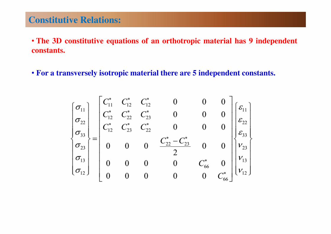
• The 3D constitutive equations of an orthotropic material has 9 independent
constants.
• For a transversely isotropic material there are 5 independent constants.
Constitutive Relations:
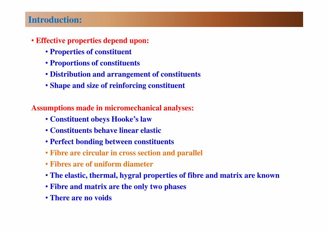
• Effective properties depend upon:
• Properties of constituent
• Proportions of constituents
• Distribution and arrangement of constituents
• Shape and size of reinforcing constituent
Assumptions made in micromechanical analyses:
• Constituent obeys Hooke’s law
• Constituents behave linear elastic
• Perfect bonding between constituents
• Fibre are circular in cross section and parallel
• Fibres are of uniform diameter
• The elastic, thermal, hygral properties of fibre and matrix are known
• Fibre and matrix are the only two phases
• There are no voids
Introduction:

• Idealization of cross-section
• Most commonly preferred arrangements are square and hexagonal packed
arrays of fibres in matrix.
Fibre Arrangement in Matrix Material:
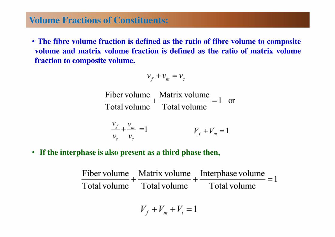
• The fibre volume fraction is defined as the ratio of fibre volume to composite
volume and matrix volume fraction is defined as the ratio of matrix volume
fraction to composite volume.
• If the interphase is also present as a third phase then,
Volume Fractions of Constituents:
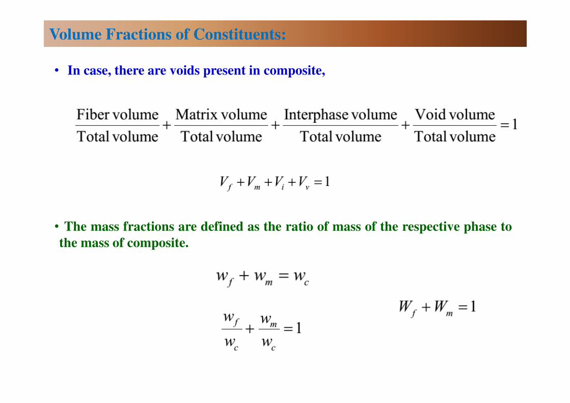
• In case, there are voids present in composite,
• The mass fractions are defined as the ratio of mass of the respective phase to
the mass of composite.
Volume Fractions of Constituents:
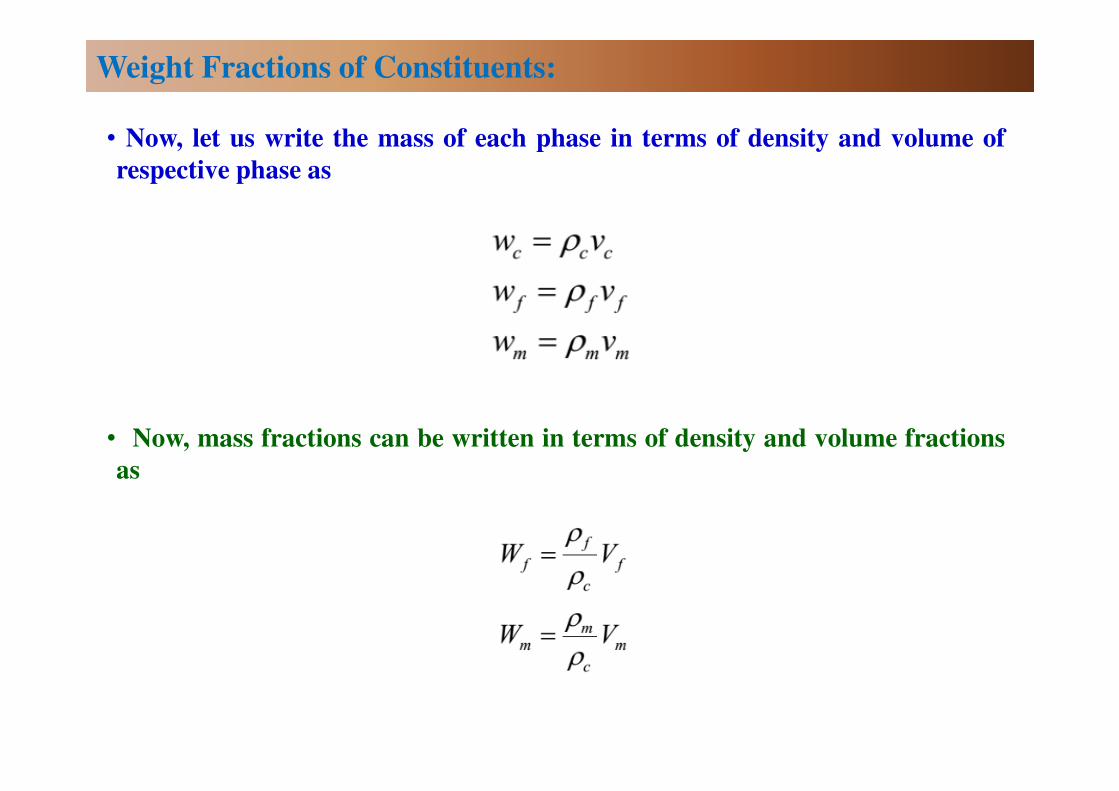
• Now, let us write the mass of each phase in terms of density and volume of
respective phase as
• Now, mass fractions can be written in terms of density and volume fractions
as
Weight Fractions of Constituents:
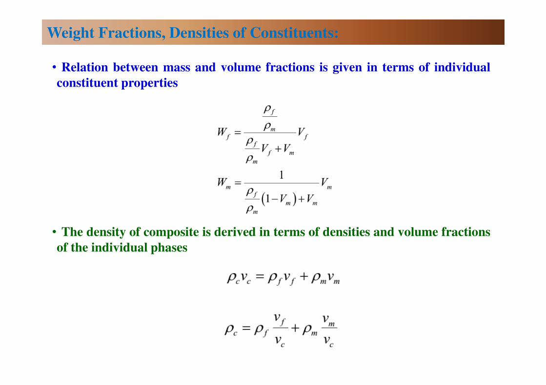
• Relation between mass and volume fractions is given in terms of individual
constituent properties
• The density of composite is derived in terms of densities and volume fractions
of the individual phases
Weight Fractions, Densities of Constituents:
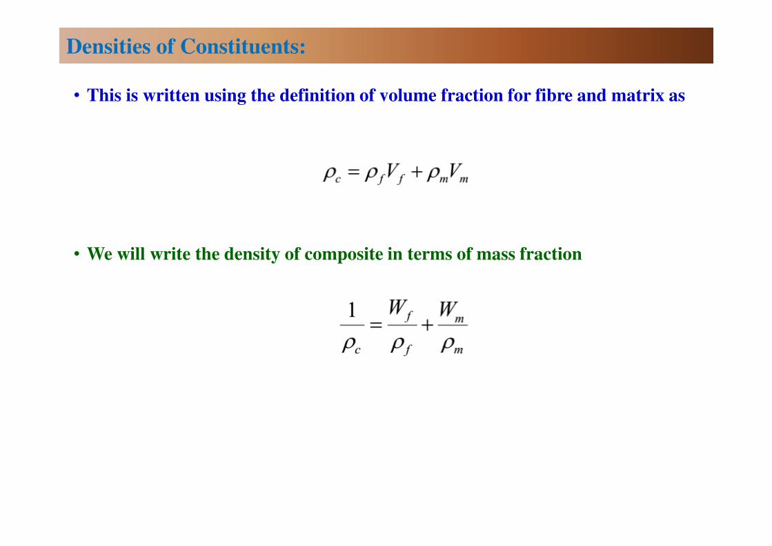
• This is written using the definition of volume fraction for fibre and matrix as
• We will write the density of composite in terms of mass fraction
Densities of Constituents:
Strength of Materials Approach
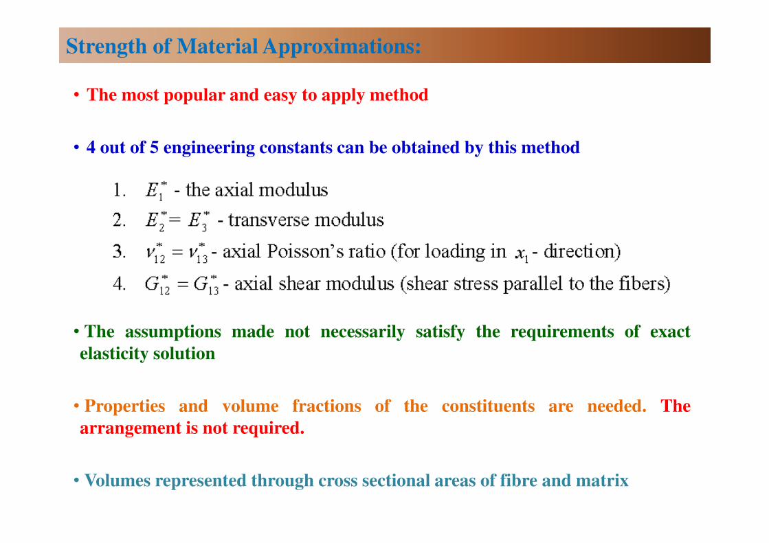
• The most popular and easy to apply method
• 4 out of 5 engineering constants can be obtained by this method
• The assumptions made not necessarily satisfy the requirements of exact
elasticity solution
• Properties and volume fractions of the constituents are needed. The
arrangement is not required.
• Volumes represented through cross sectional areas of fibre and matrix
Strength of Material Approximations:
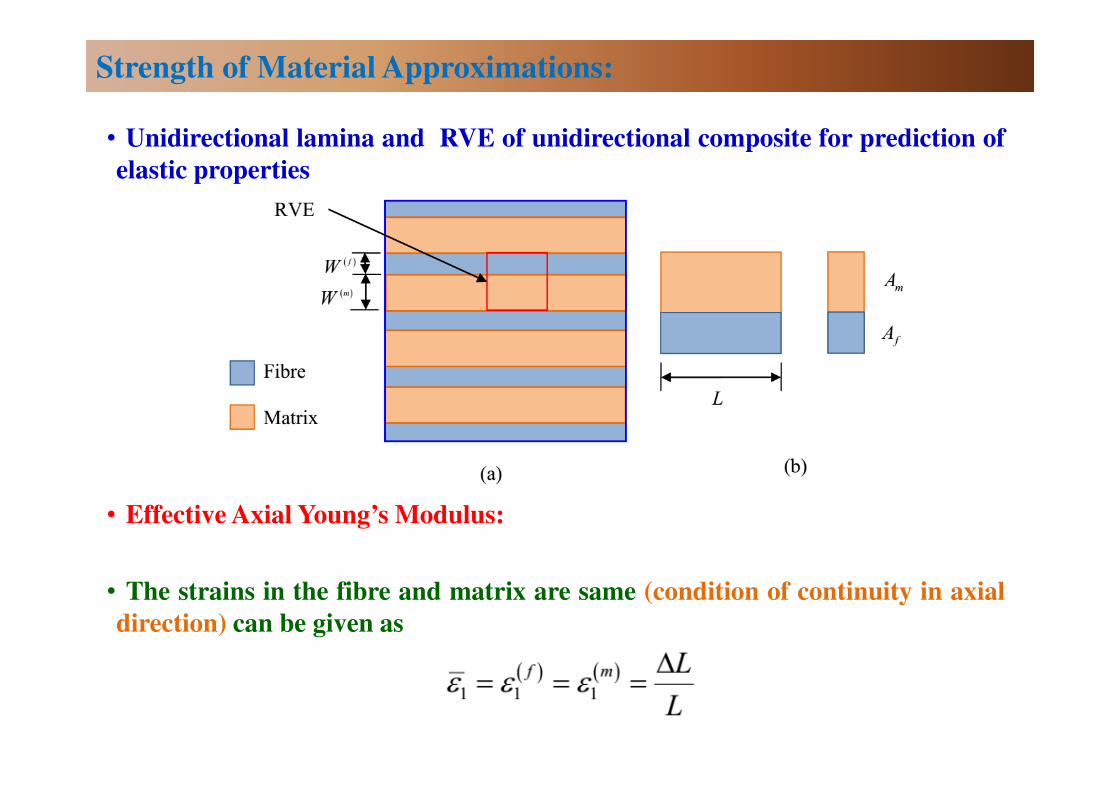
• Unidirectional lamina and RVE of unidirectional composite for prediction of
elastic properties
• Effective Axial Young’s Modulus:
• The strains in the fibre and matrix are same (condition of continuity in axial
direction) can be given as
Strength of Material Approximations:
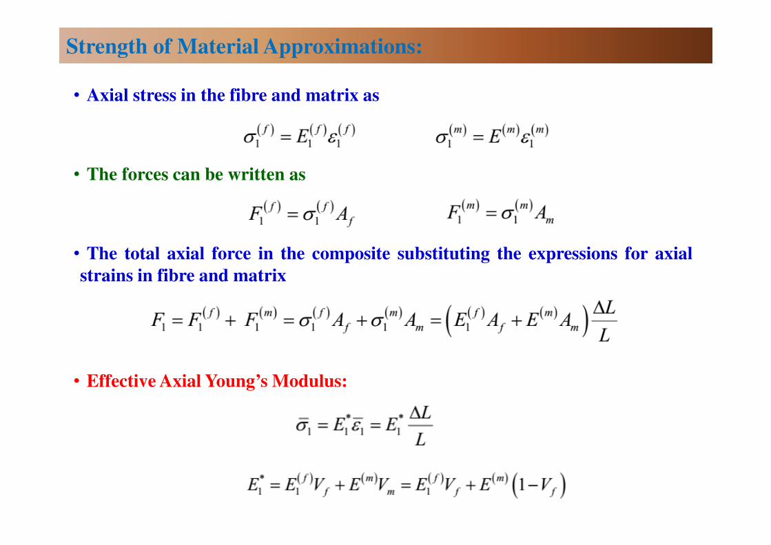
• Axial stress in the fibre and matrix as
• The forces can be written as
• The total axial force in the composite substituting the expressions for axial
strains in fibre and matrix
• Effective Axial Young’s Modulus:
Strength of Material Approximations:

• Undeformed unit cell under average axial stress and deformed individual
constituents of the unit cell
Strength of Material Approximations:
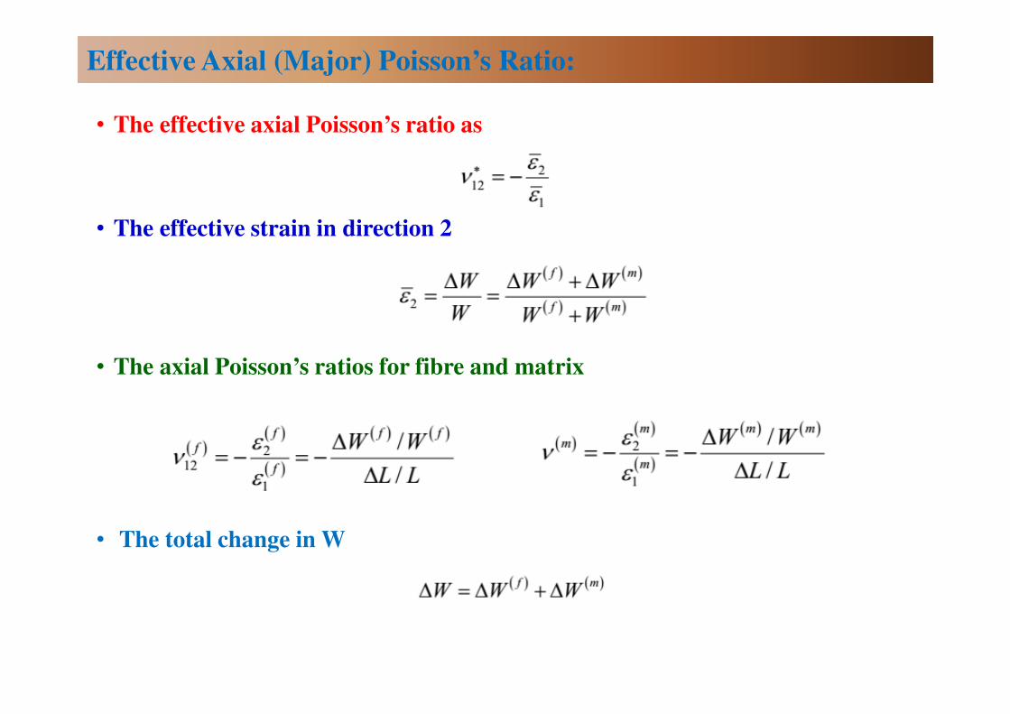
• The effective axial Poisson’s ratio as
• The effective strain in direction 2
• The axial Poisson’s ratios for fibre and matrix
• The total change in W
Effective Axial (Major) Poisson’s Ratio:
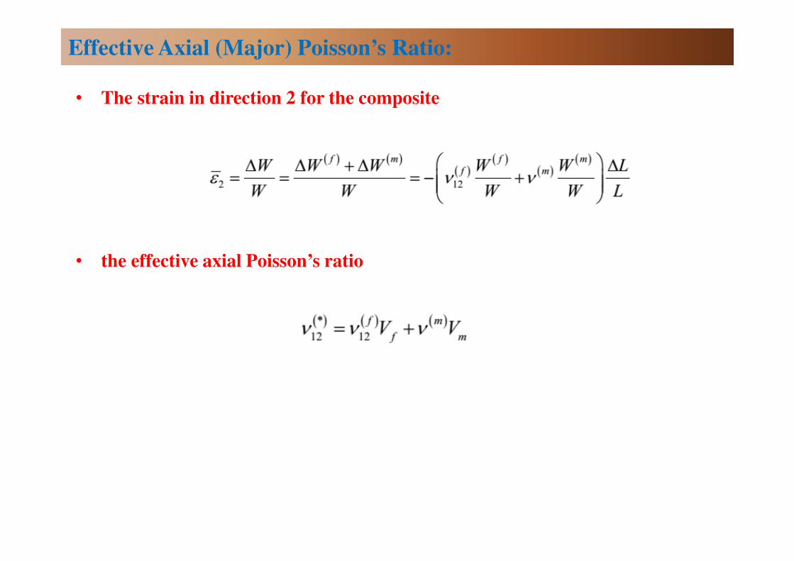
• The strain in direction 2 for the composite
• the effective axial Poisson’s ratio
Effective Axial (Major) Poisson’s Ratio:
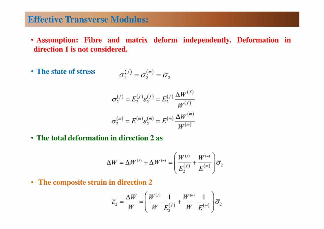
• Assumption: Fibre and matrix deform independently. Deformation in
direction 1 is not considered.
• The state of stress
• The total deformation in direction 2 as
• The composite strain in direction 2
Effective Transverse Modulus:
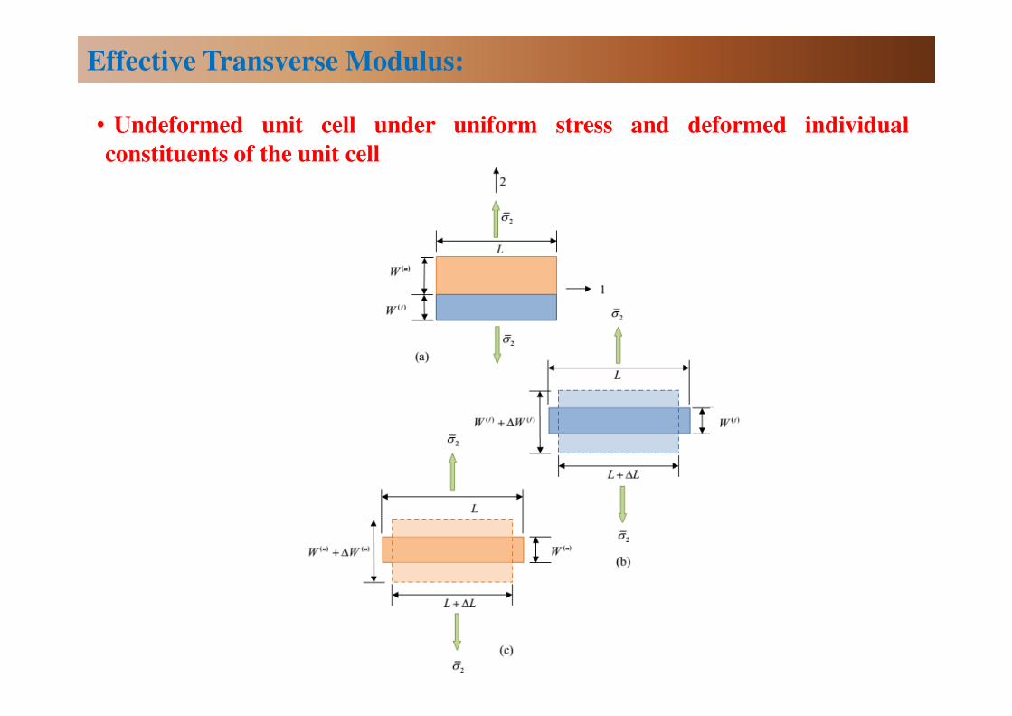
• Undeformed unit cell under uniform stress and deformed individual
constituents of the unit cell
Effective Transverse Modulus:
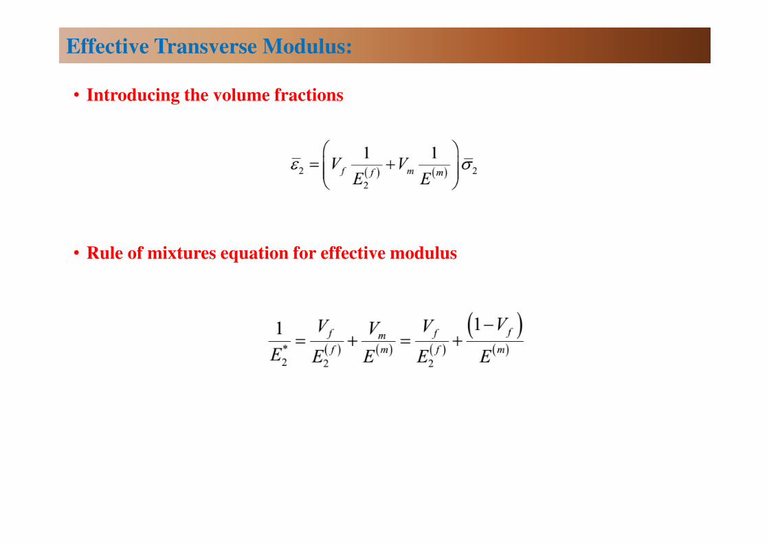
• Introducing the volume fractions
• Rule of mixtures equation for effective modulus
Effective Transverse Modulus:
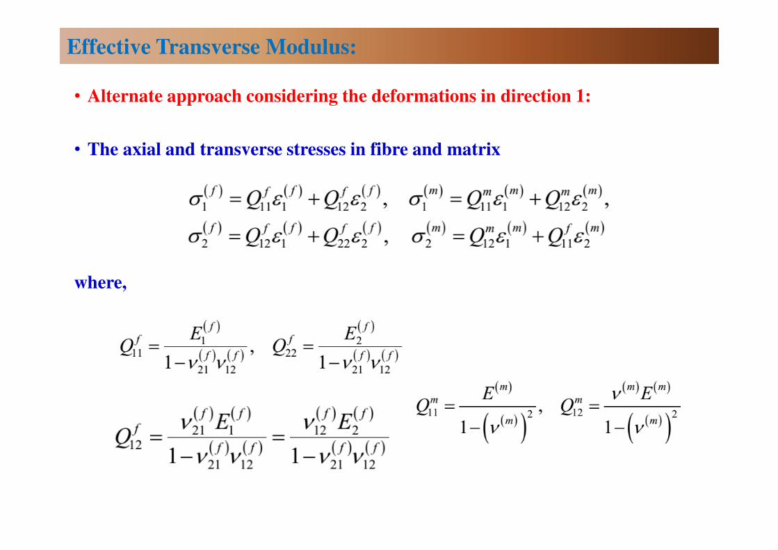
• Alternate approach considering the deformations in direction 1:
• The axial and transverse stresses in fibre and matrix
where,
Effective Transverse Modulus:
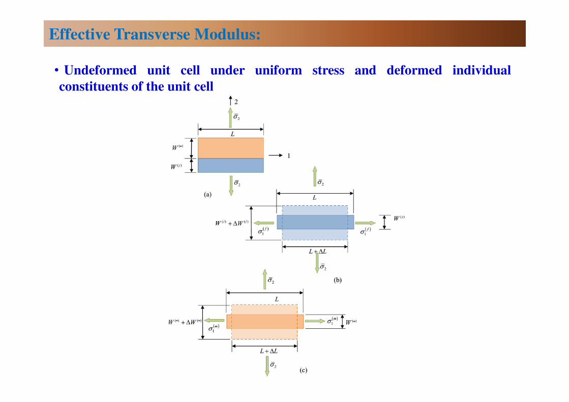
• Undeformed unit cell under uniform stress and deformed individual
constituents of the unit cell
Effective Transverse Modulus:
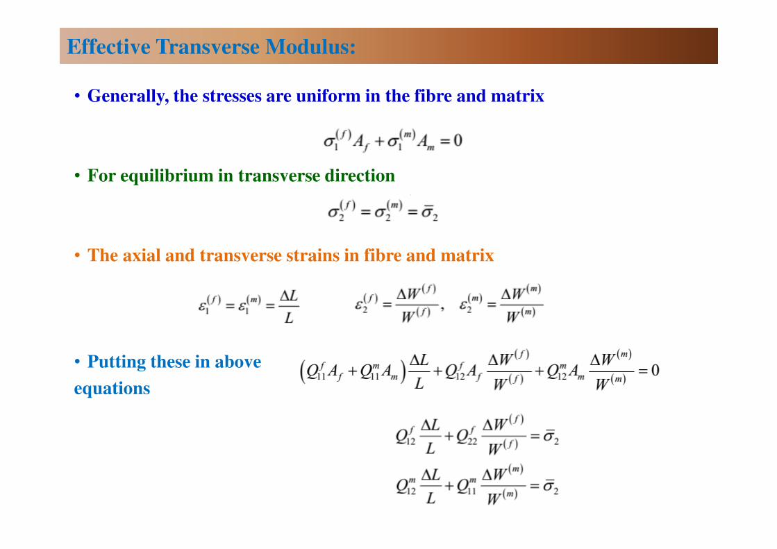
• Generally, the stresses are uniform in the fibre and matrix
• For equilibrium in transverse direction
• The axial and transverse strains in fibre and matrix
• Putting these in above
equations
Effective Transverse Modulus:
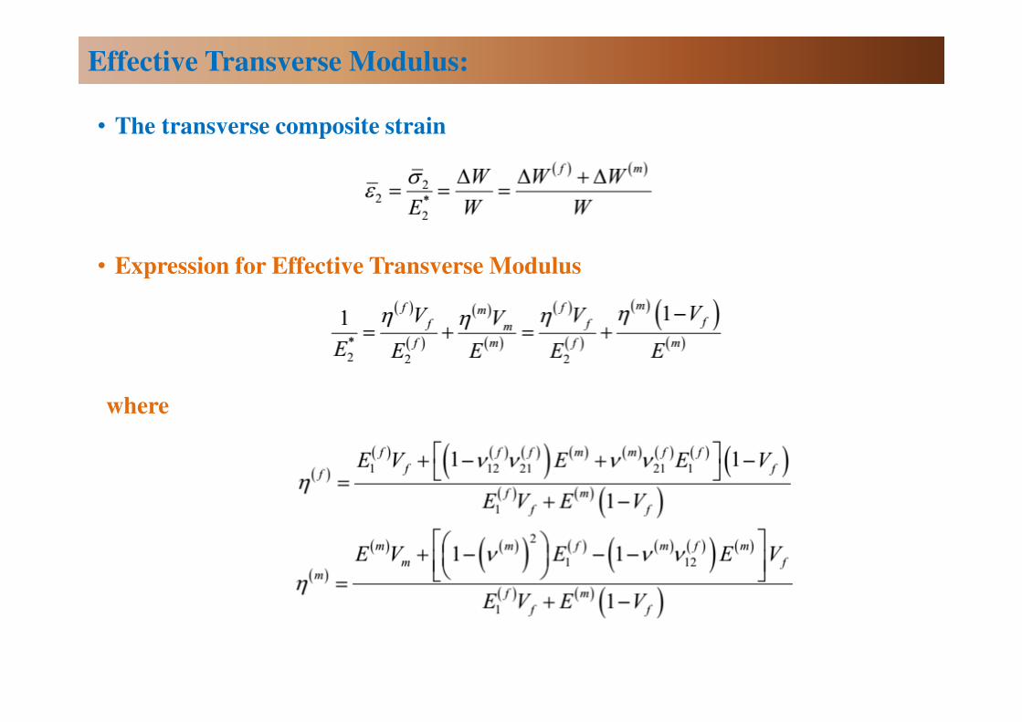
• The transverse composite strain
• Expression for Effective Transverse Modulus
where
Effective Transverse Modulus:
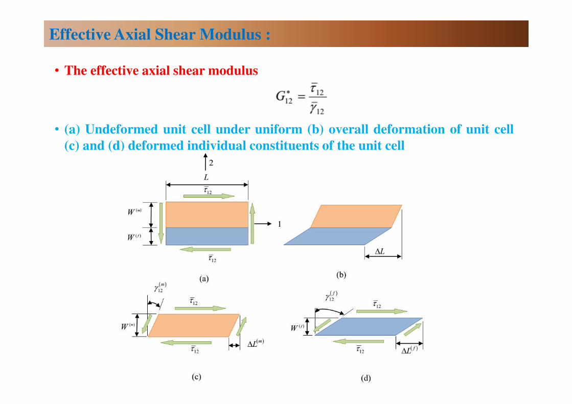
• The effective axial shear modulus
• (a) Undeformed unit cell under uniform (b) overall deformation of unit cell
(c) and (d) deformed individual constituents of the unit cell
Effective Axial Shear Modulus :
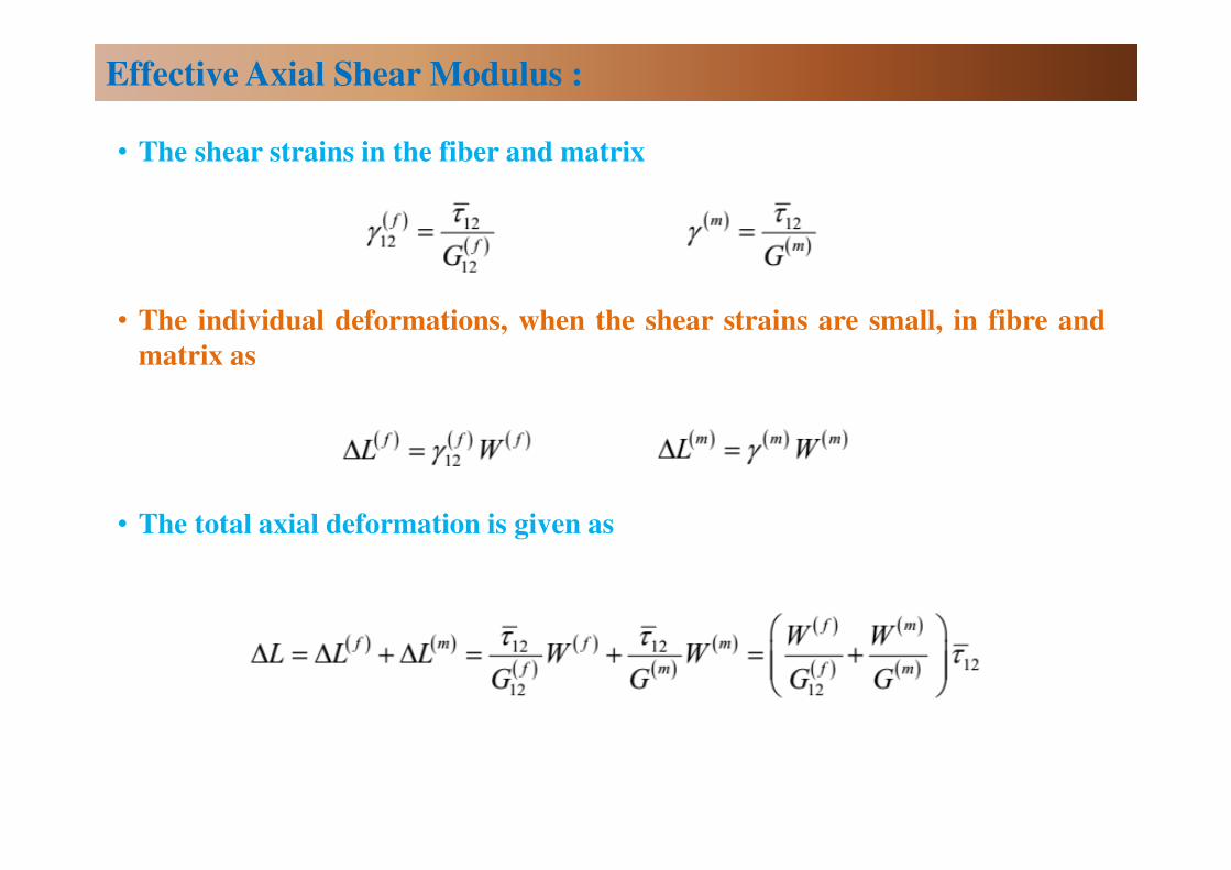
• The shear strains in the fiber and matrix
• The individual deformations, when the shear strains are small, in fibre and
matrix as
• The total axial deformation is given as
Effective Axial Shear Modulus :
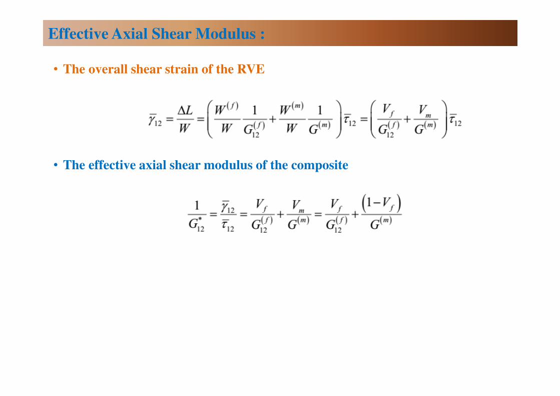
• The overall shear strain of the RVE
• The effective axial shear modulus of the composite
Effective Axial Shear Modulus :
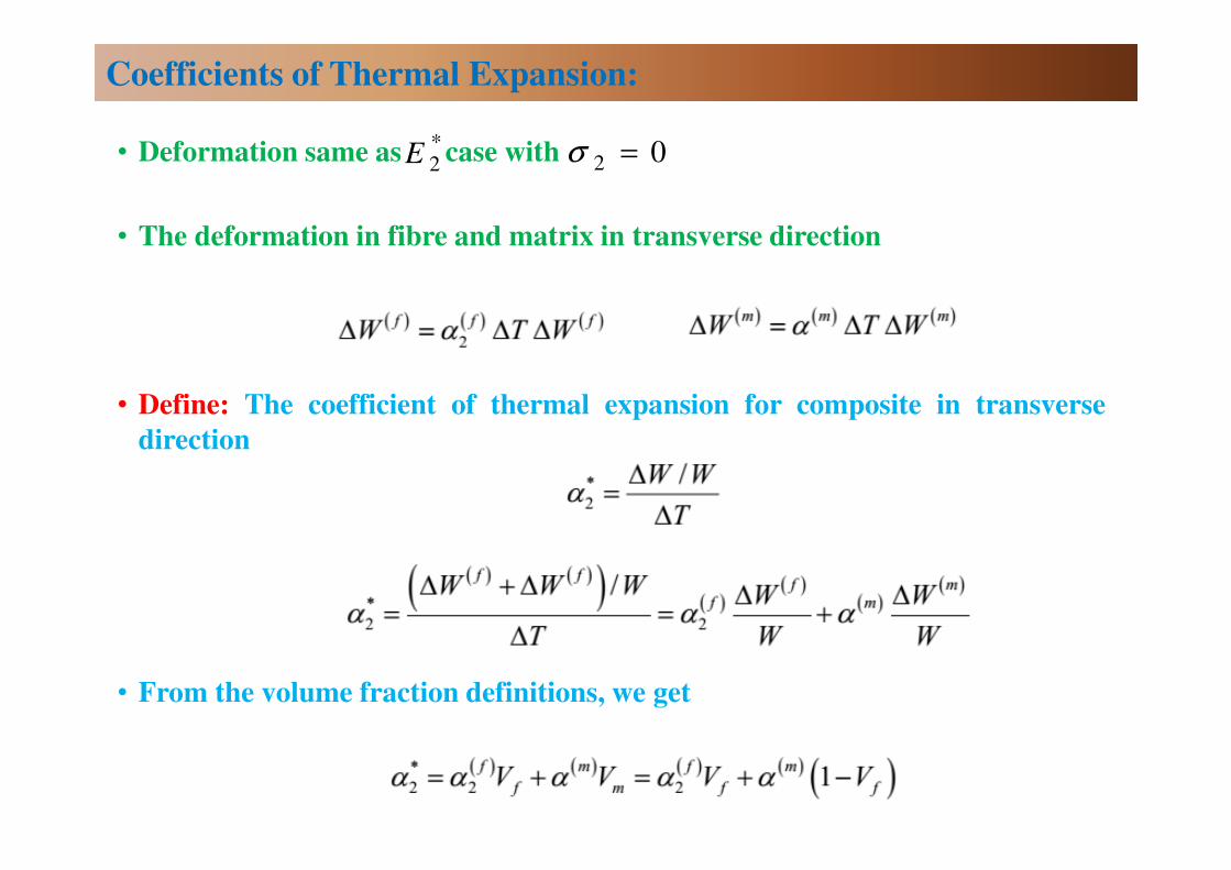
• Deformation same as case with
• The deformation in fibre and matrix in transverse direction
• Define: The coefficient of thermal expansion for composite in transverse
direction
• From the volume fraction definitions, we get
Coefficients of Thermal Expansion:
*
2E 2 0σ =
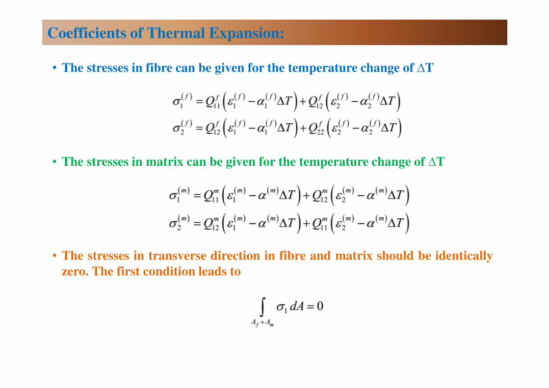
• The stresses in fibre can be given for the temperature change of ȂT
• The stresses in matrix can be given for the temperature change of ȂT
• The stresses in transverse direction in fibre and matrix should be identically
zero. The first condition leads to
Coefficients of Thermal Expansion:
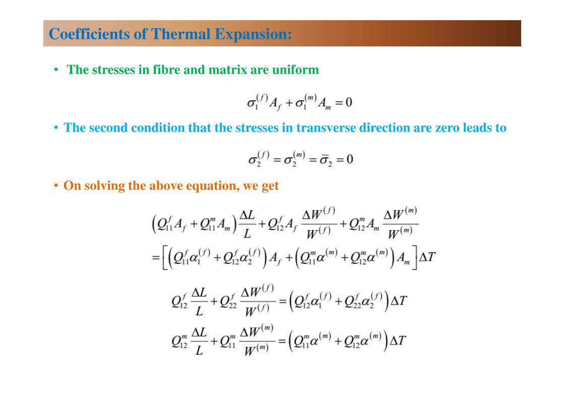
• The stresses in fibre and matrix are uniform
• The second condition that the stresses in transverse direction are zero leads to
• On solving the above equation, we get
Coefficients of Thermal Expansion:
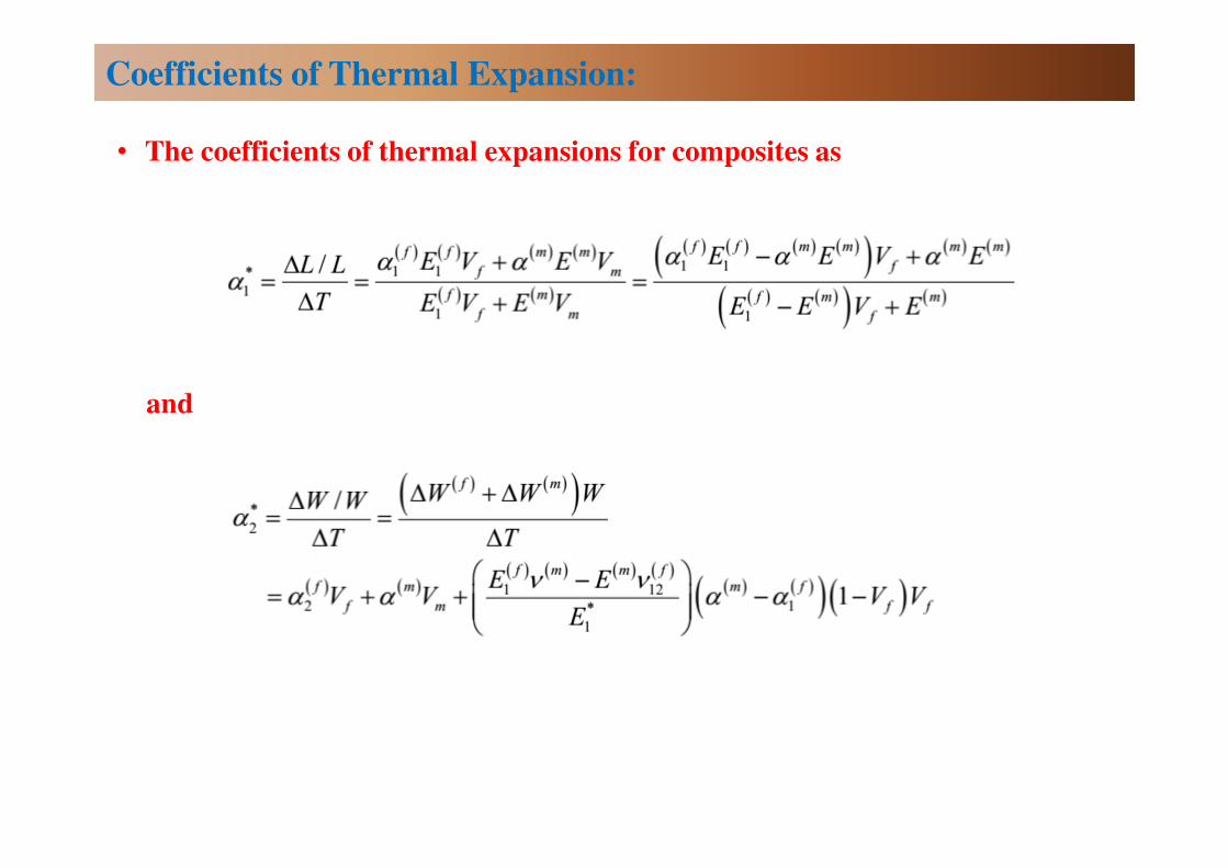
• The coefficients of thermal expansions for composites as
and
Coefficients of Thermal Expansion:
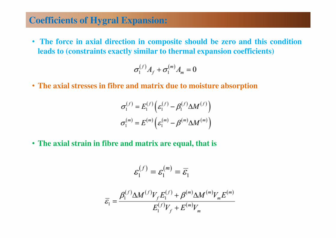
• The force in axial direction in composite should be zero and this condition
leads to (constraints exactly similar to thermal expansion coefficients)
• The axial stresses in fibre and matrix due to moisture absorption
• The axial strain in fibre and matrix are equal, that is
Coefficients of Hygral Expansion:
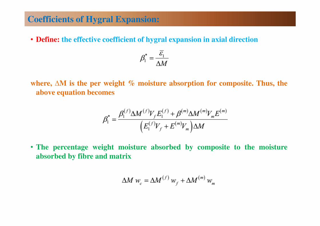
• Define: the effective coefficient of hygral expansion in axial direction
where, ȂM is the per weight % moisture absorption for composite. Thus, the
above equation becomes
• The percentage weight moisture absorbed by composite to the moisture
absorbed by fibre and matrix
Coefficients of Hygral Expansion:
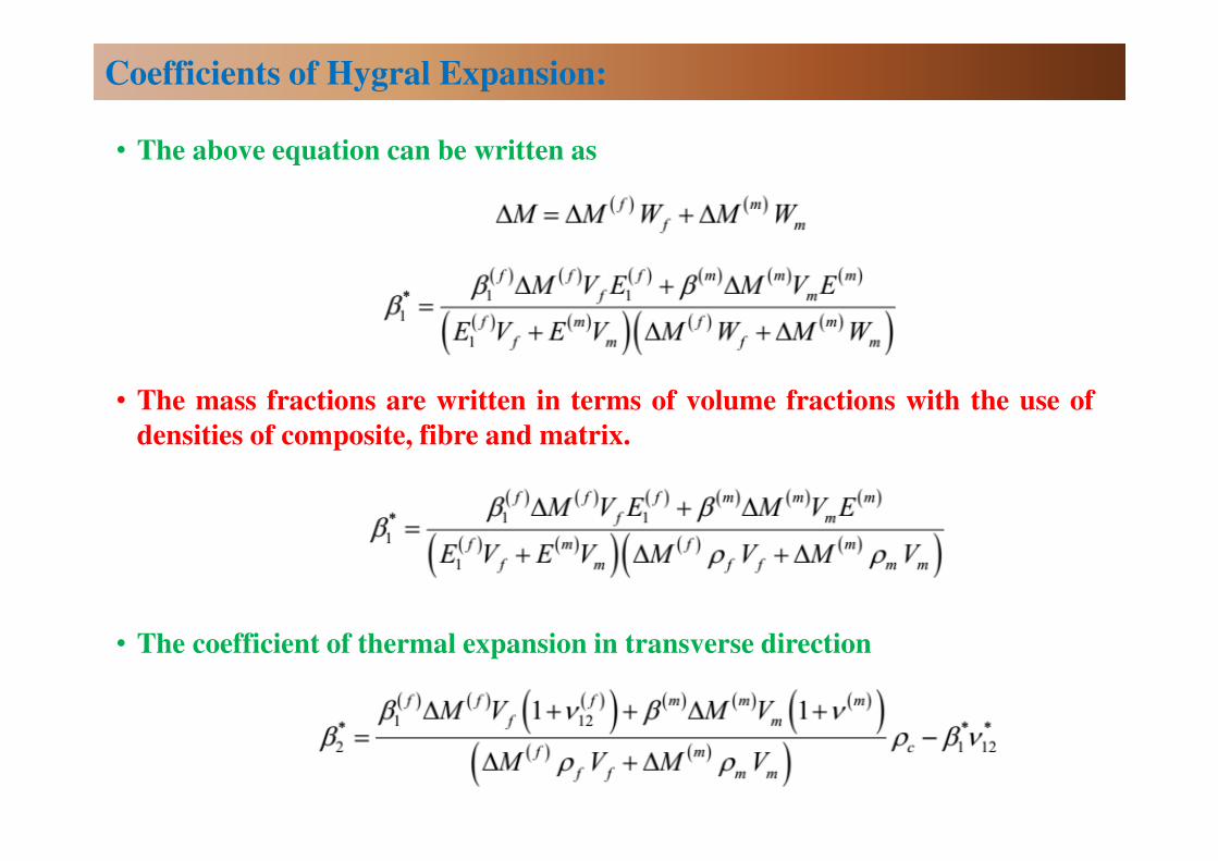
• The above equation can be written as
• The mass fractions are written in terms of volume fractions with the use of
densities of composite, fibre and matrix.
• The coefficient of thermal expansion in transverse direction
Coefficients of Hygral Expansion:
Statistical Homogeneity

• Scale of inhomogeneity and averaging of properties along with an RVE
(a) continuous variation of heterogeneity
(b) abrupt variation of heterogeneity
λ – characteristic dimension of
inhomogeneity
δ – length scale of averaging
δ>> λ
δ – must be large enough to represent the microstructural details and
interaction between fibres and matrix.
Other terms: effective, equivalent, macroscopic or statistical homogeneity
The Concept of Equivalent Homogeneity:
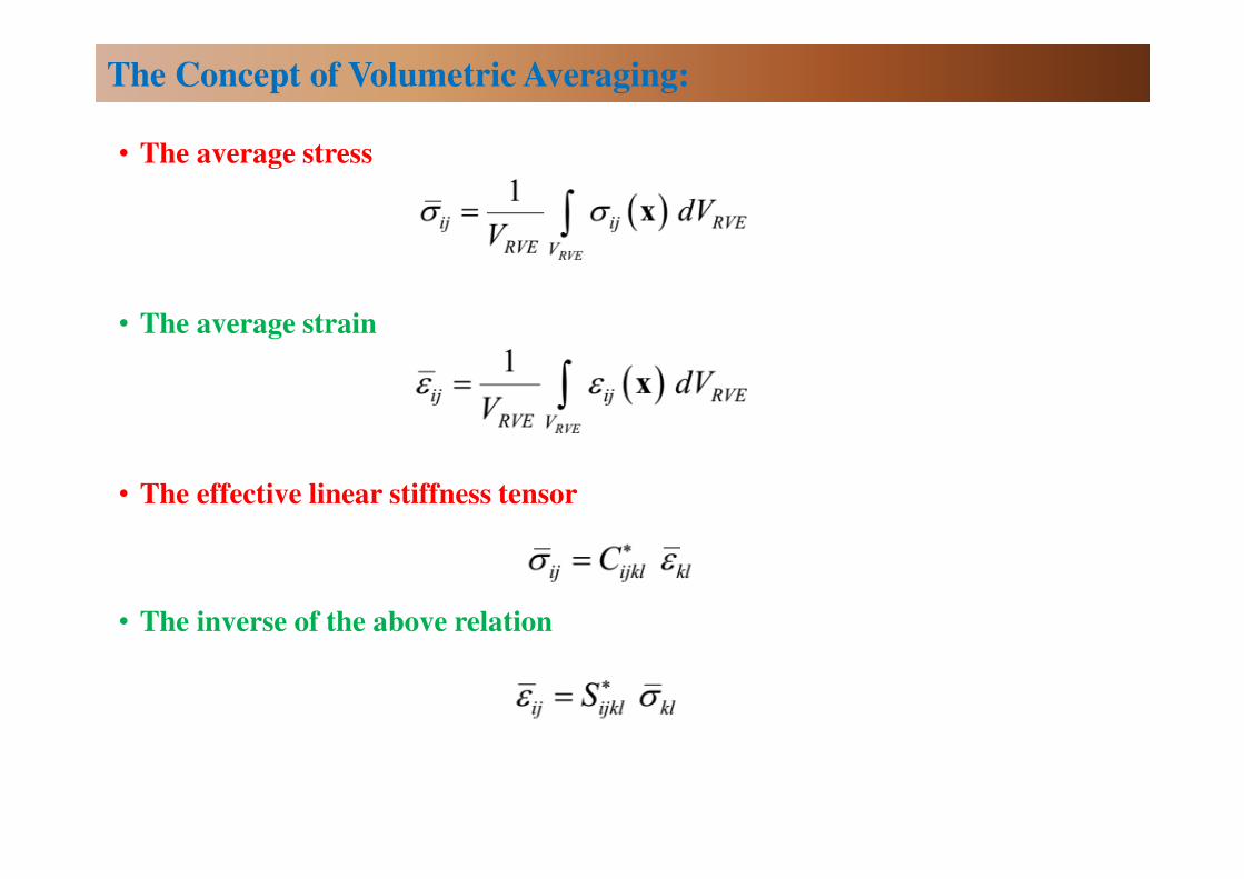
• The average stress
• The average strain
• The effective linear stiffness tensor
• The inverse of the above relation
The Concept of Volumetric Averaging:
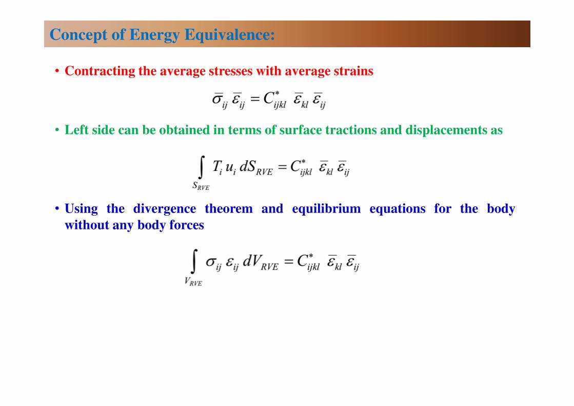
Concept of Energy Equivalence:
• Contracting the average stresses with average strains
• Left side can be obtained in terms of surface tractions and displacements as
• Using the divergence theorem and equilibrium equations for the body
without any body forces
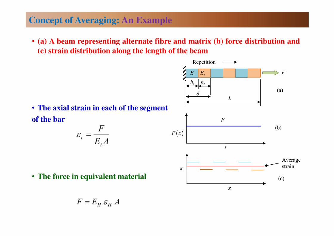
• (a) A beam representing alternate fibre and matrix (b) force distribution and
(c) strain distribution along the length of the beam
• The axial strain in each of the segment
of the bar
• The force in equivalent material
Concept of Averaging: An Example
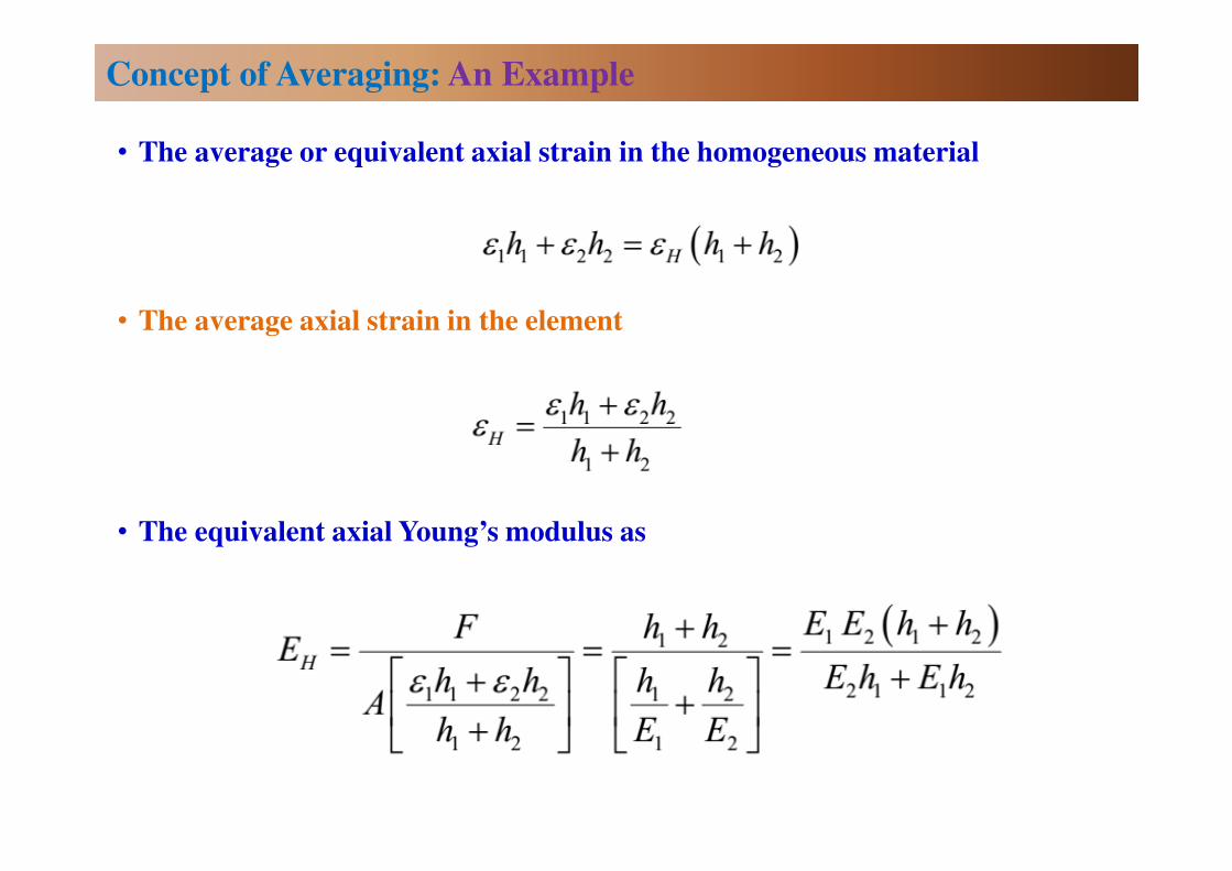
• The average or equivalent axial strain in the homogeneous material
• The average axial strain in the element
• The equivalent axial Young’s modulus as
Concept of Averaging: An Example

• The strain energies of the non-homogeneous and homogeneous materials
which upon simplification gives
Concept of Averaging: An Example
Standard Mechanics Approach
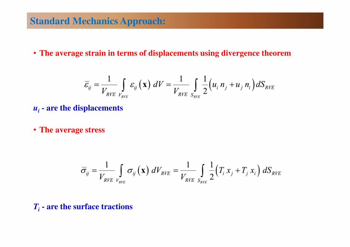
• The average strain in terms of displacements using divergence theorem
ui - are the displacements
• The average stress
Ti - are the surface tractions
Standard Mechanics Approach:

• Boundary conditions that produce average strain or stress
• Uniform boundary conditions on an RVE
• In case of the applied displacements the weak form of the RVE equilibrium
equations
Standard Mechanics Approach:
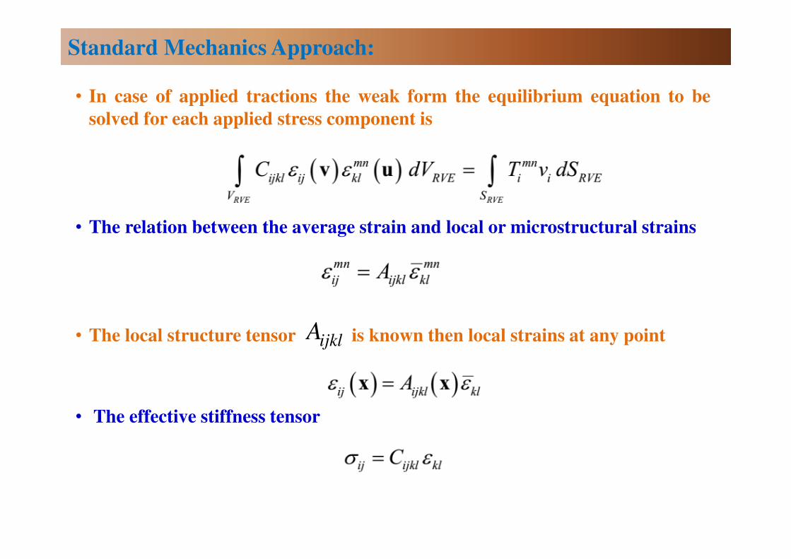
• In case of applied tractions the weak form the equilibrium equation to be
solved for each applied stress component is
• The relation between the average strain and local or microstructural strains
• The local structure tensor is known then local strains at any point
• The effective stiffness tensor
Standard Mechanics Approach:
ijklA
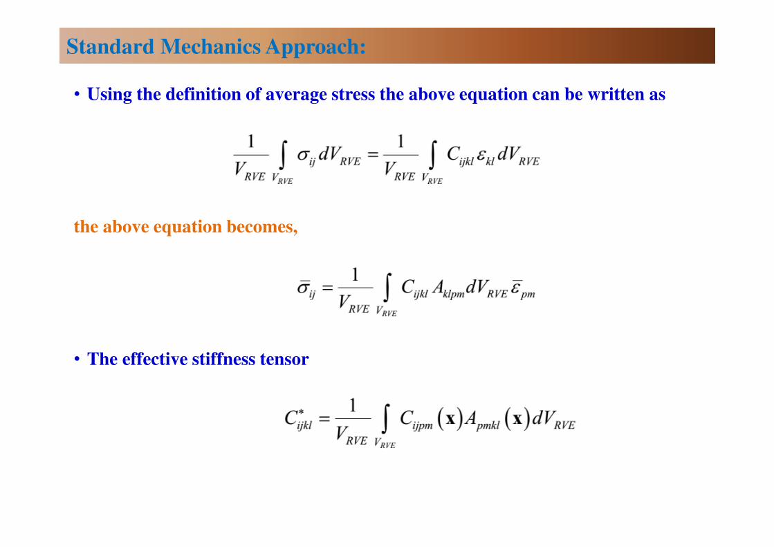
• Using the definition of average stress the above equation can be written as
the above equation becomes,
• The effective stiffness tensor
Standard Mechanics Approach:
Hills Concentration Factors Approach
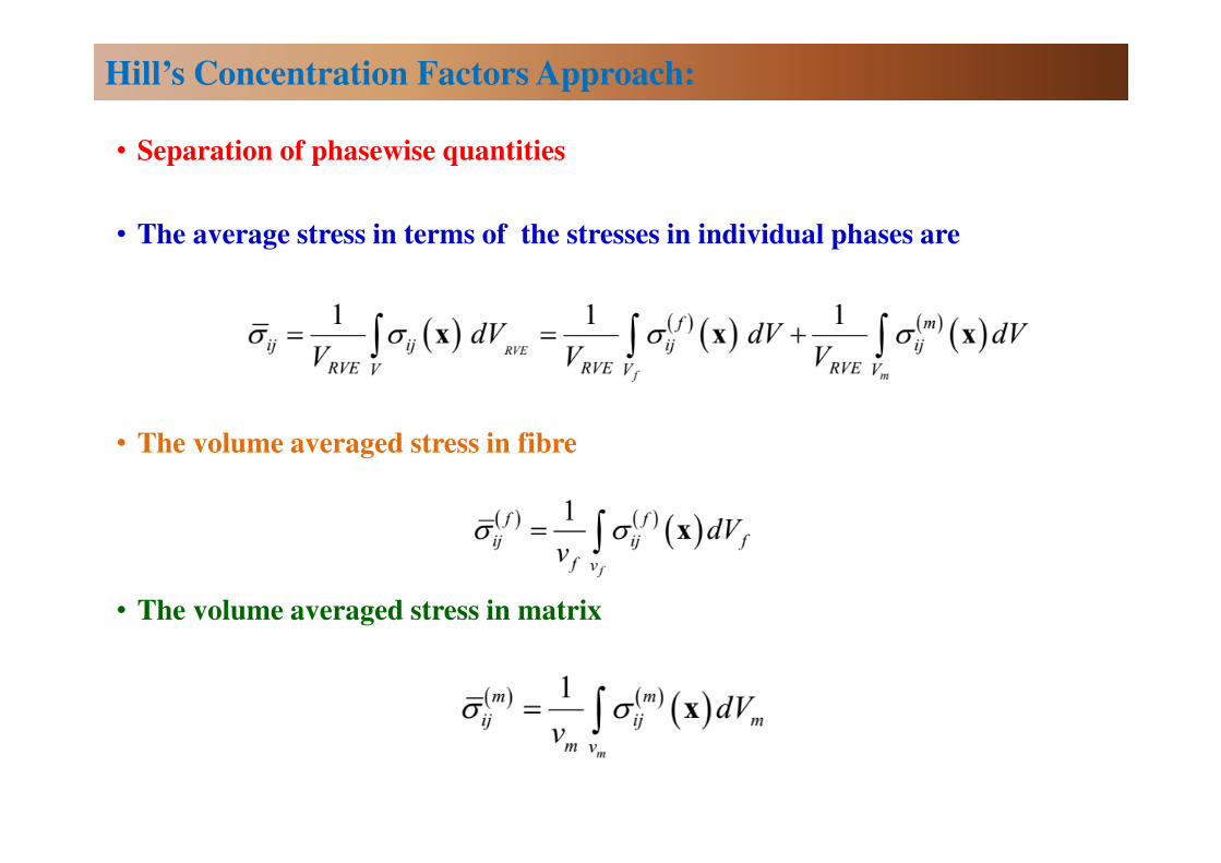
• Separation of phasewise quantities
• The average stress in terms of the stresses in individual phases are
• The volume averaged stress in fibre
• The volume averaged stress in matrix
Hill’s Concentration Factors Approach:
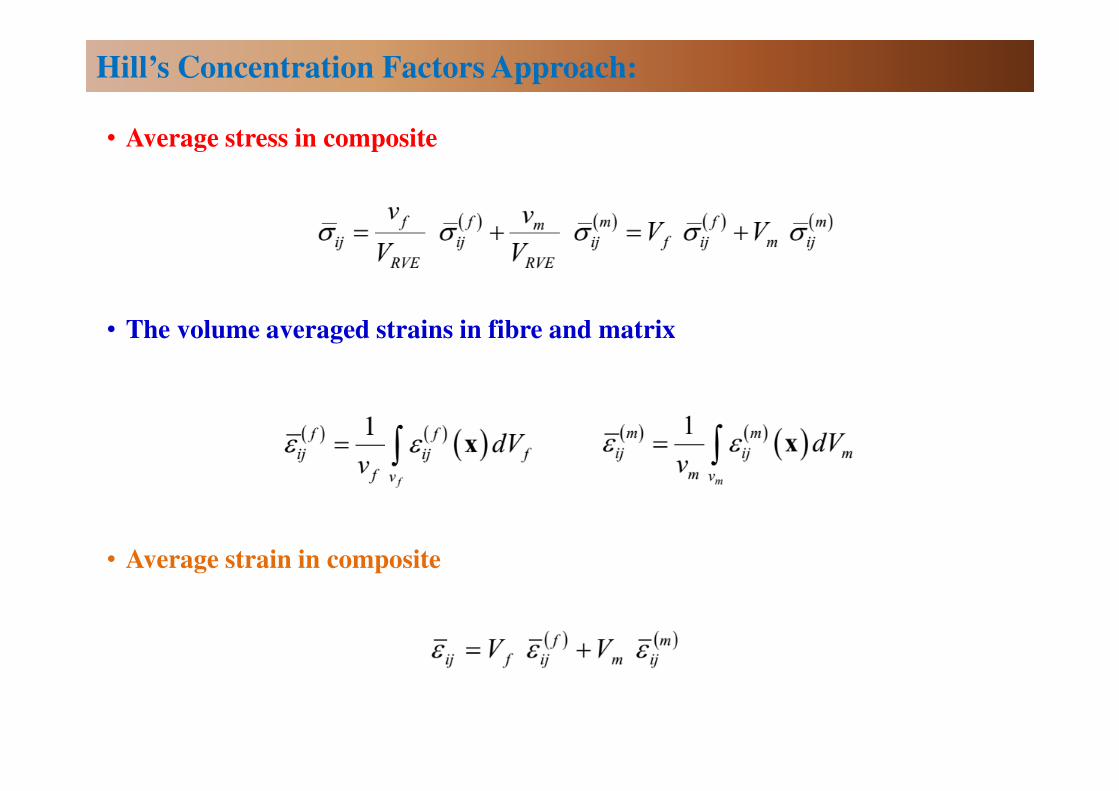
• Average stress in composite
• The volume averaged strains in fibre and matrix
• Average strain in composite
Hill’s Concentration Factors Approach:
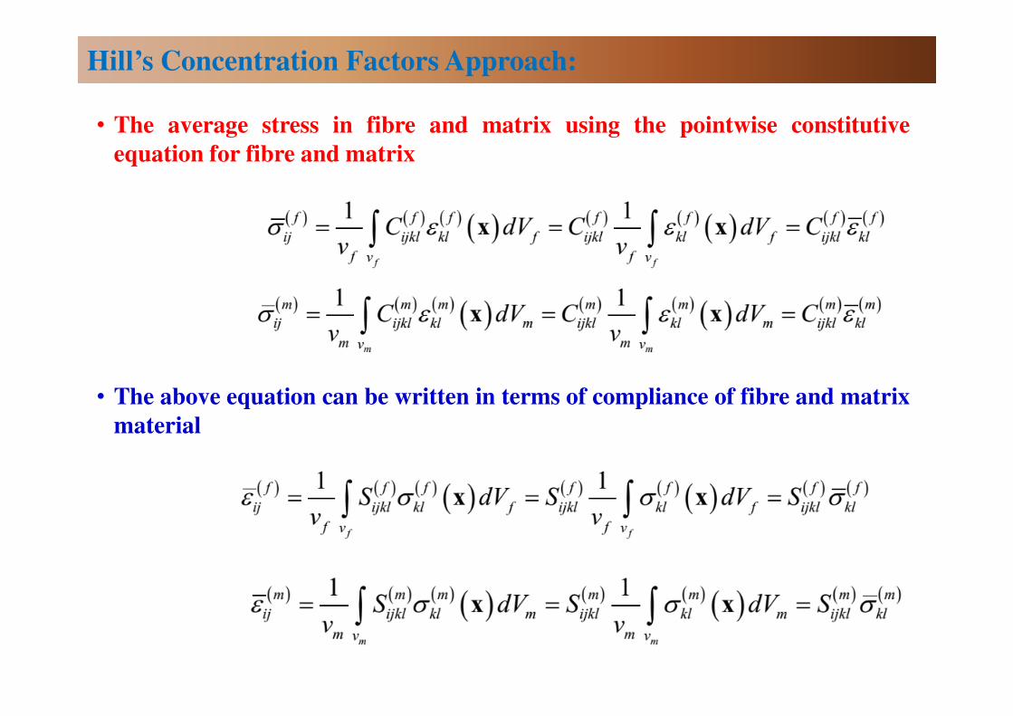
• The average stress in fibre and matrix using the pointwise constitutive
equation for fibre and matrix
• The above equation can be written in terms of compliance of fibre and matrix
material
Hill’s Concentration Factors Approach:
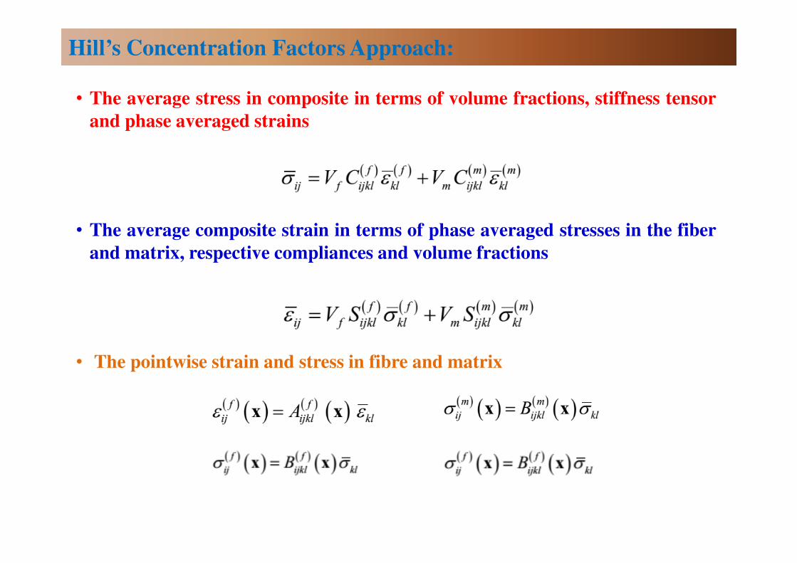
• The average stress in composite in terms of volume fractions, stiffness tensor
and phase averaged strains
• The average composite strain in terms of phase averaged stresses in the fiber
and matrix, respective compliances and volume fractions
• The pointwise strain and stress in fibre and matrix
Hill’s Concentration Factors Approach:
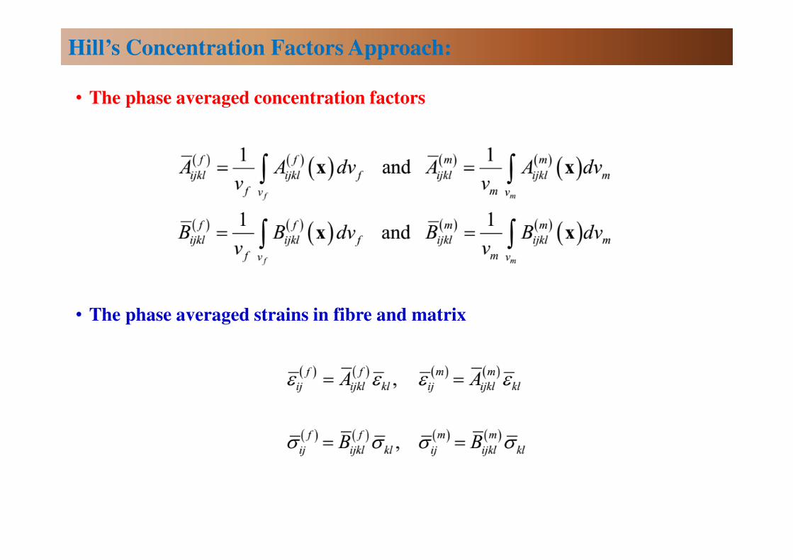
• The phase averaged concentration factors
• The phase averaged strains in fibre and matrix
Hill’s Concentration Factors Approach:
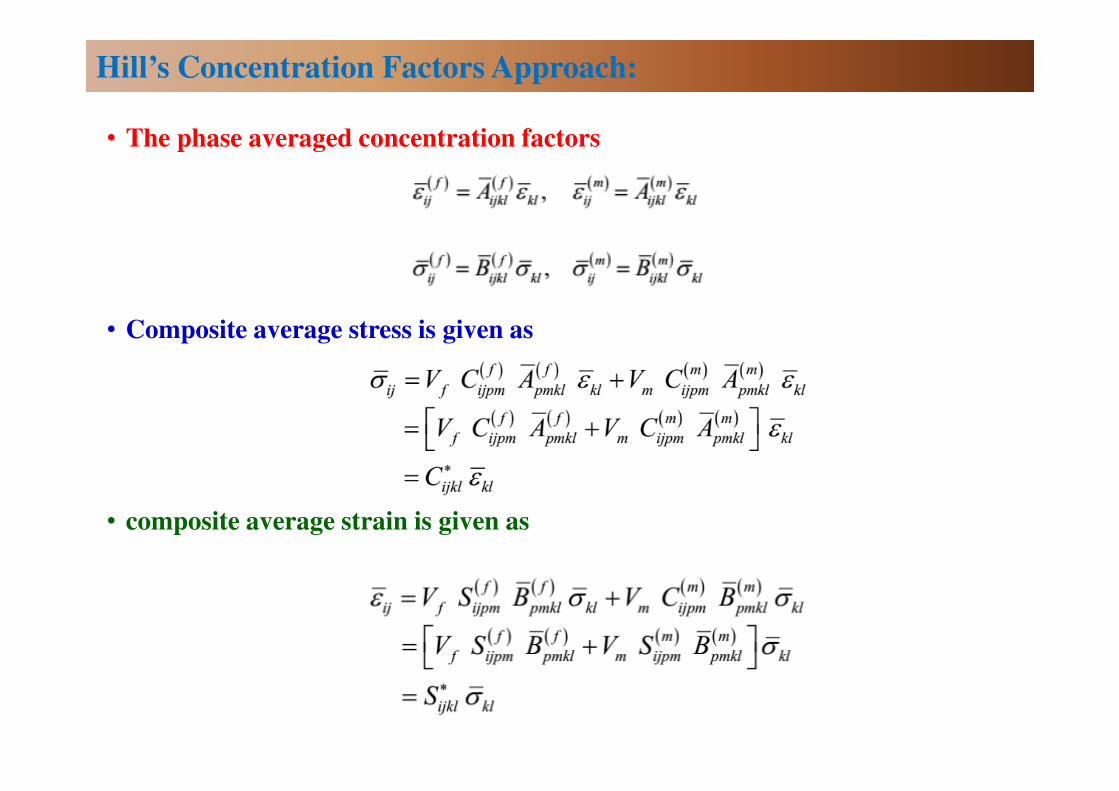
• The phase averaged concentration factors
• Composite average stress is given as
• composite average strain is given as
Hill’s Concentration Factors Approach:
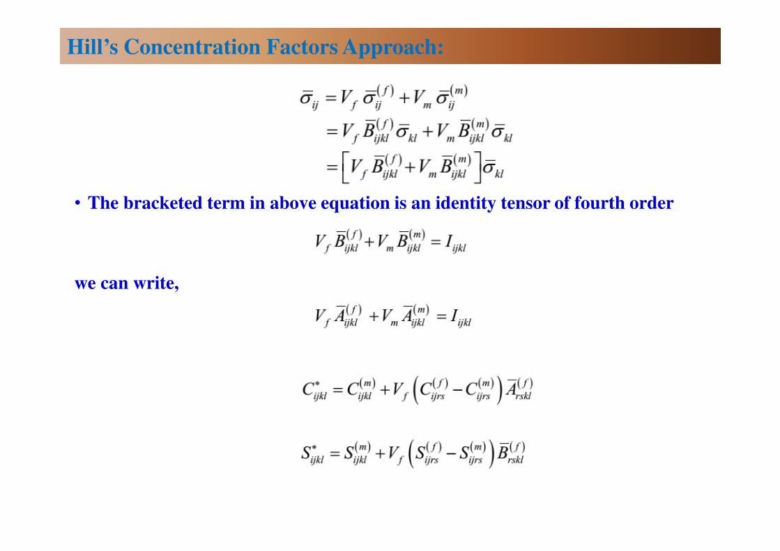
• The bracketed term in above equation is an identity tensor of fourth order
we can write,
Hill’s Concentration Factors Approach:

• Voigt assumed that the strains are constants throughout the composite
this leads to,
• We can write,
Voigt Approximation:
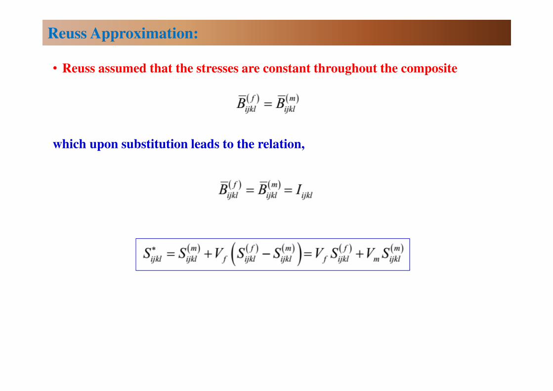
• Reuss assumed that the stresses are constant throughout the composite
which upon substitution leads to the relation,
Reuss Approximation:
Mathematical Theory of
Homogenization

• (a) A bar representing alternate fibre and matrix (b) actual and average
strain (c) actual and average displacement and (d) periodic nature of
displacement difference over RVE length
Concept of Homogenization:
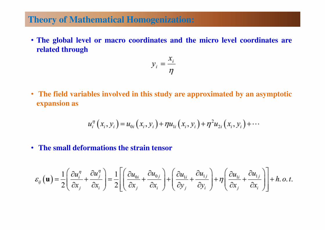
• The global level or macro coordinates and the micro level coordinates are
related through
• The field variables involved in this study are approximated by an asymptotic
expansion as
• The small deformations the strain tensor
Theory of Mathematical Homogenization:
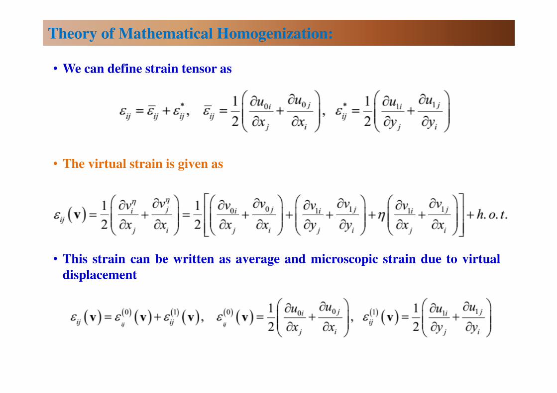
• We can define strain tensor as
• The virtual strain is given as
• This strain can be written as average and microscopic strain due to virtual
displacement
Theory of Mathematical Homogenization:
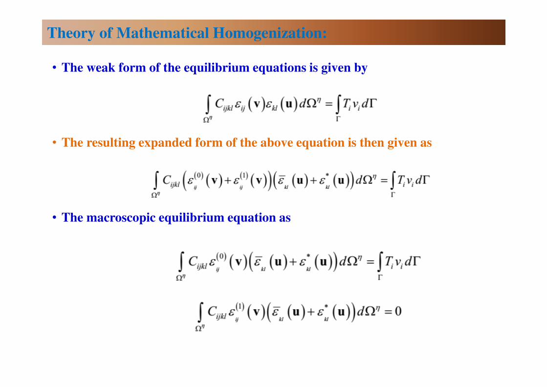
• The weak form of the equilibrium equations is given by
• The resulting expanded form of the above equation is then given as
• The macroscopic equilibrium equation as
Theory of Mathematical Homogenization:

• The above equation may be simplified assuming η approaching zero in the
limit as
and
• In the above equation the integration term over the RVE should be zero, this
leads to the following condition:
Theory of Mathematical Homogenization:
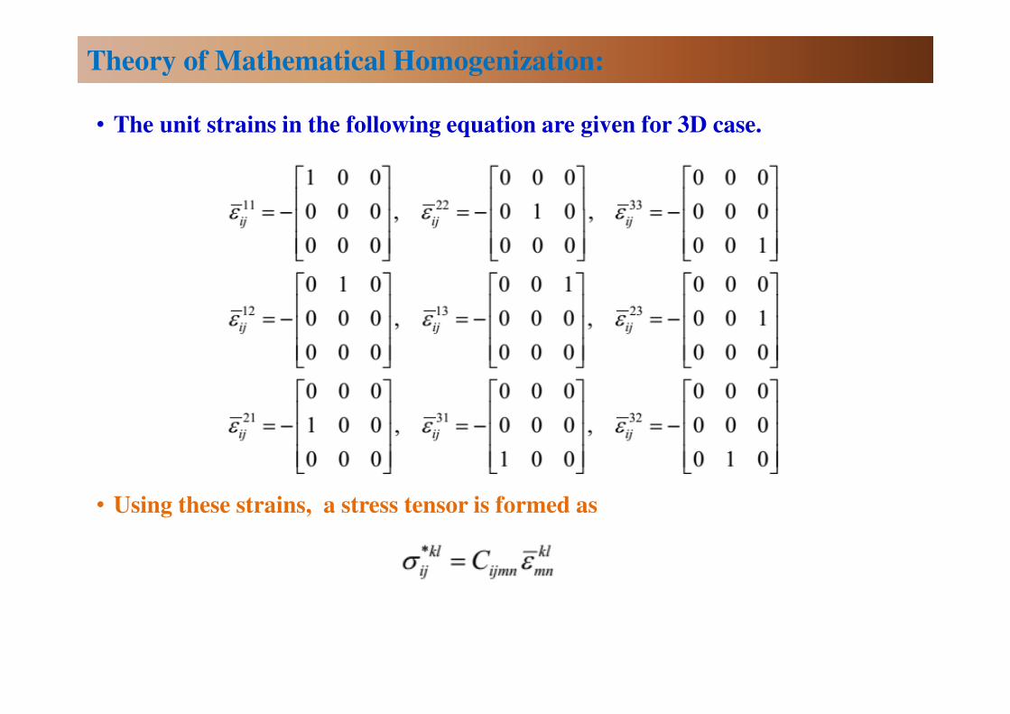
• The unit strains in the following equation are given for 3D case.
• Using these strains, a stress tensor is formed as
Theory of Mathematical Homogenization:
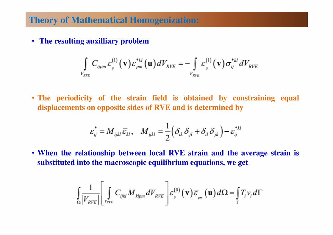
• The resulting auxilliary problem
• The periodicity of the strain field is obtained by constraining equal
displacements on opposite sides of RVE and is determined by
• When the relationship between local RVE strain and the average strain is
substituted into the macroscopic equilibrium equations, we get
Theory of Mathematical Homogenization:
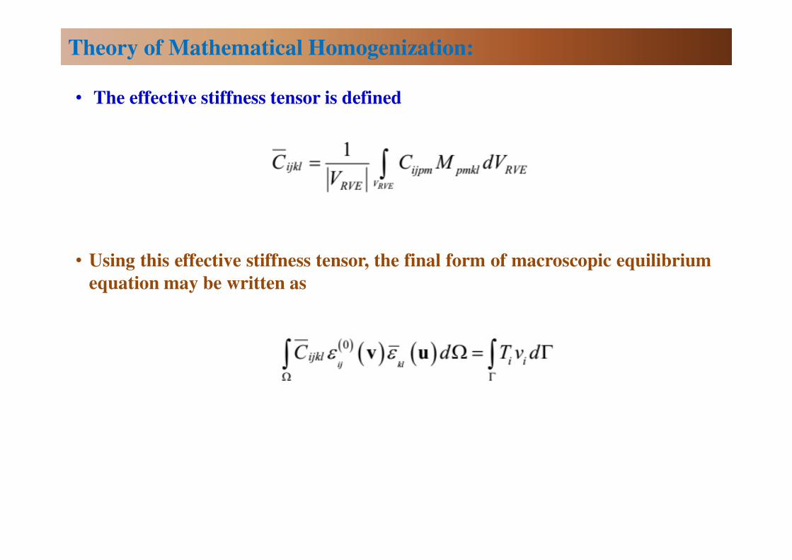
• The effective stiffness tensor is defined
• Using this effective stiffness tensor, the final form of macroscopic equilibrium
equation may be written as
Theory of Mathematical Homogenization:
Concentric Cylinder Assemblage
Model
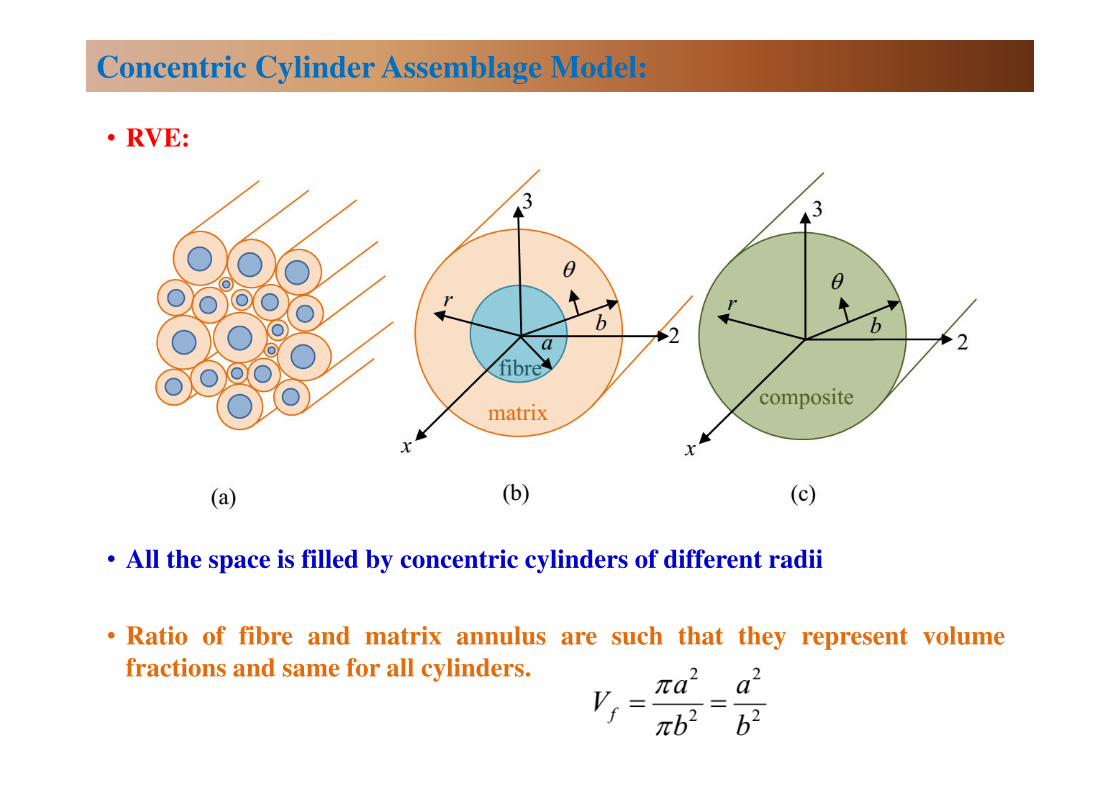
• RVE:
• All the space is filled by concentric cylinders of different radii
• Ratio of fibre and matrix annulus are such that they represent volume
fractions and same for all cylinders.
Concentric Cylinder Assemblage Model:
Background to Concentric Cylinder Assemblage Model:
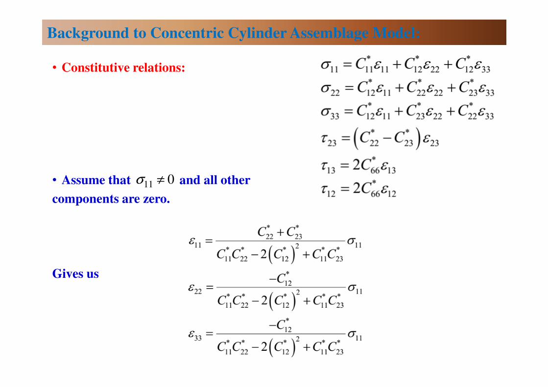
• Constitutive relations:
• Assume that and all other
components are zero.
Gives us
11 0σ ≠

Background to Concentric Cylinder Assemblage Model:
• From the relation
• Define
to give
• Similarly, define
which gives
Further, we get
Background to Concentric Cylinder Assemblage Model:
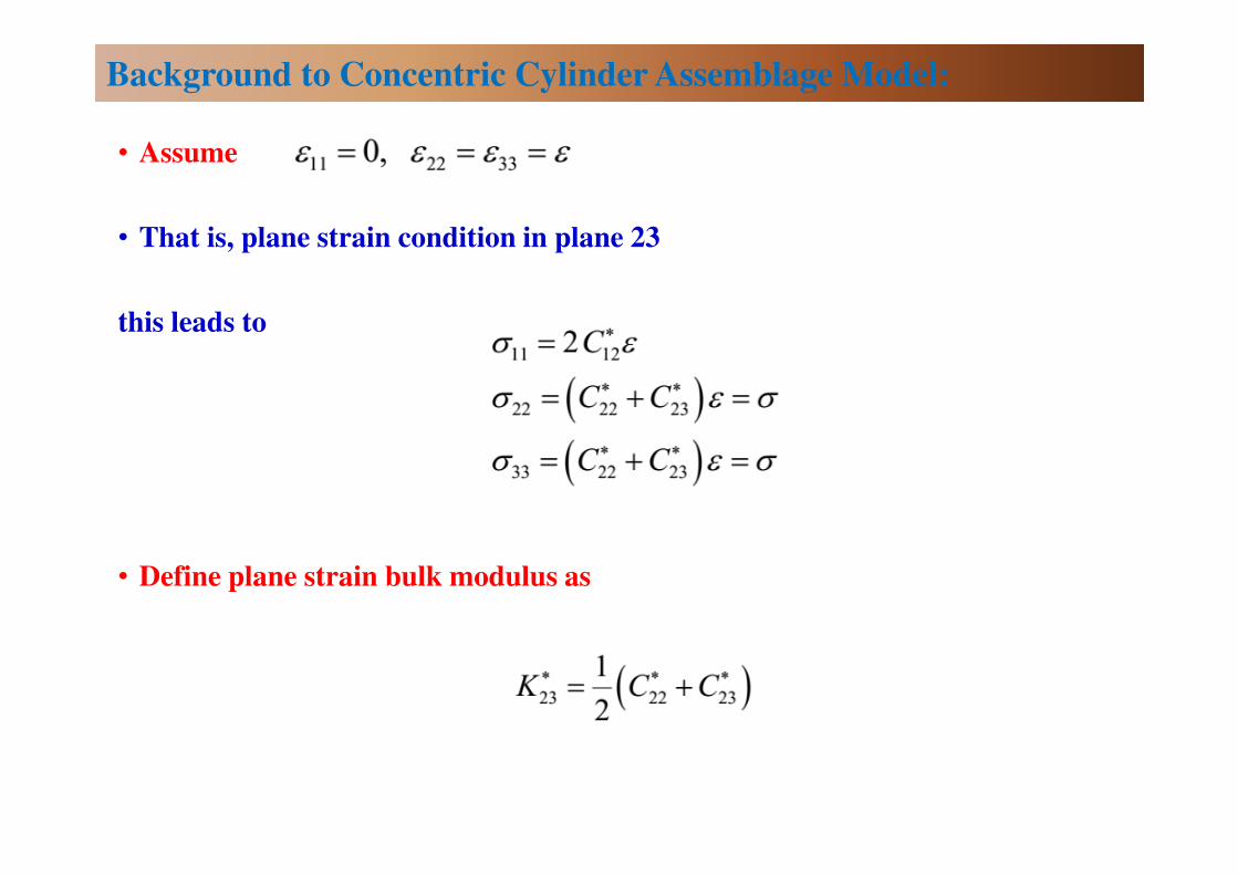
• Assume
• That is, plane strain condition in plane 23
this leads to
• Define plane strain bulk modulus as

• Finally, we get all constants
in terms of four engineering
constants!
• Other engineering constants can be obtained indirectly.
Let and all other
stresses be zero.
Background to Concentric Cylinder Assemblage Model:
22 0σ ≠

• From the second equation define
• Similarly, define
which gives
• Further,
Background to Concentric Cylinder Assemblage Model:
Background to Concentric Cylinder Assemblage Model:
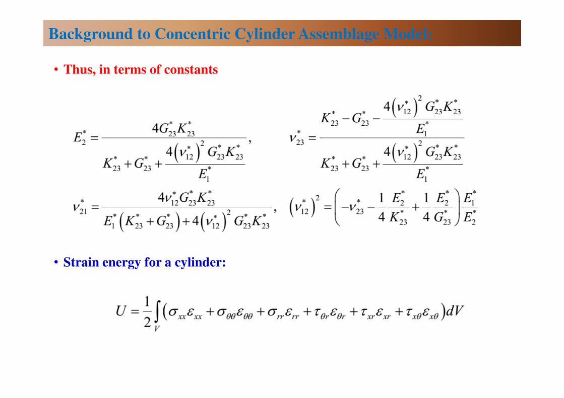
• Thus, in terms of constants
• Strain energy for a cylinder:
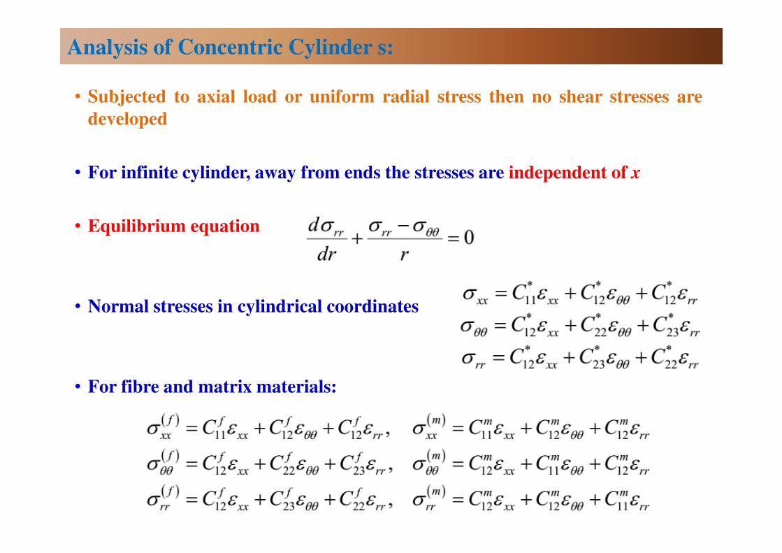
• Subjected to axial load or uniform radial stress then no shear stresses are
developed
• For infinite cylinder, away from ends the stresses are independent of x
• Equilibrium equation
• Normal stresses in cylindrical coordinates
• For fibre and matrix materials:
Analysis of Concentric Cylinder s:
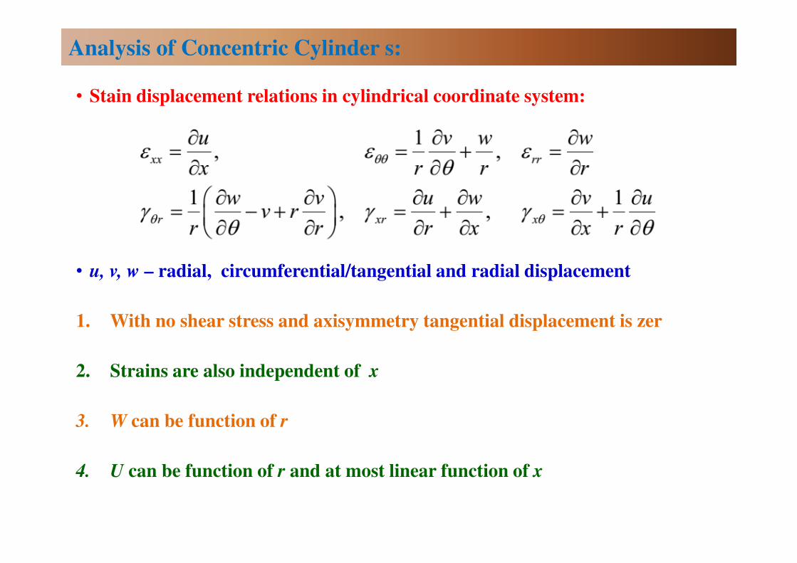
• Stain displacement relations in cylindrical coordinate system:
• u, v, w – radial, circumferential/tangential and radial displacement
1. With no shear stress and axisymmetry tangential displacement is zer
2. Strains are also independent of x
3. W can be function of r
4. U can be function of r and at most linear function of x
Analysis of Concentric Cylinder s:
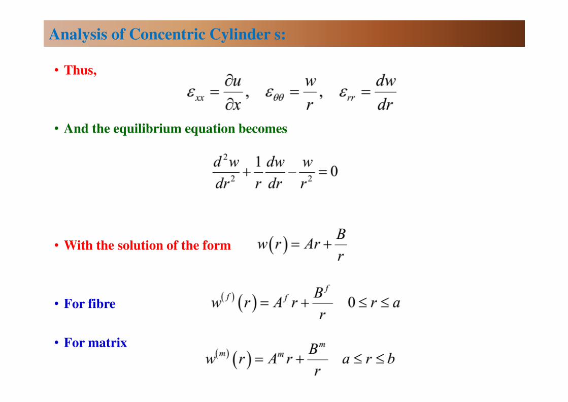
• Thus,
• And the equilibrium equation becomes
• With the solution of the form
• For fibre
• For matrix
Analysis of Concentric Cylinder s:
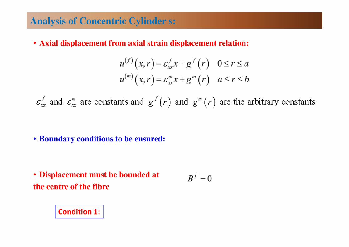
• Axial displacement from axial strain displacement relation:
• Boundary conditions to be ensured:
• Displacement must be bounded at
the centre of the fibre
Analysis of Concentric Cylinder s:
Condition 1:
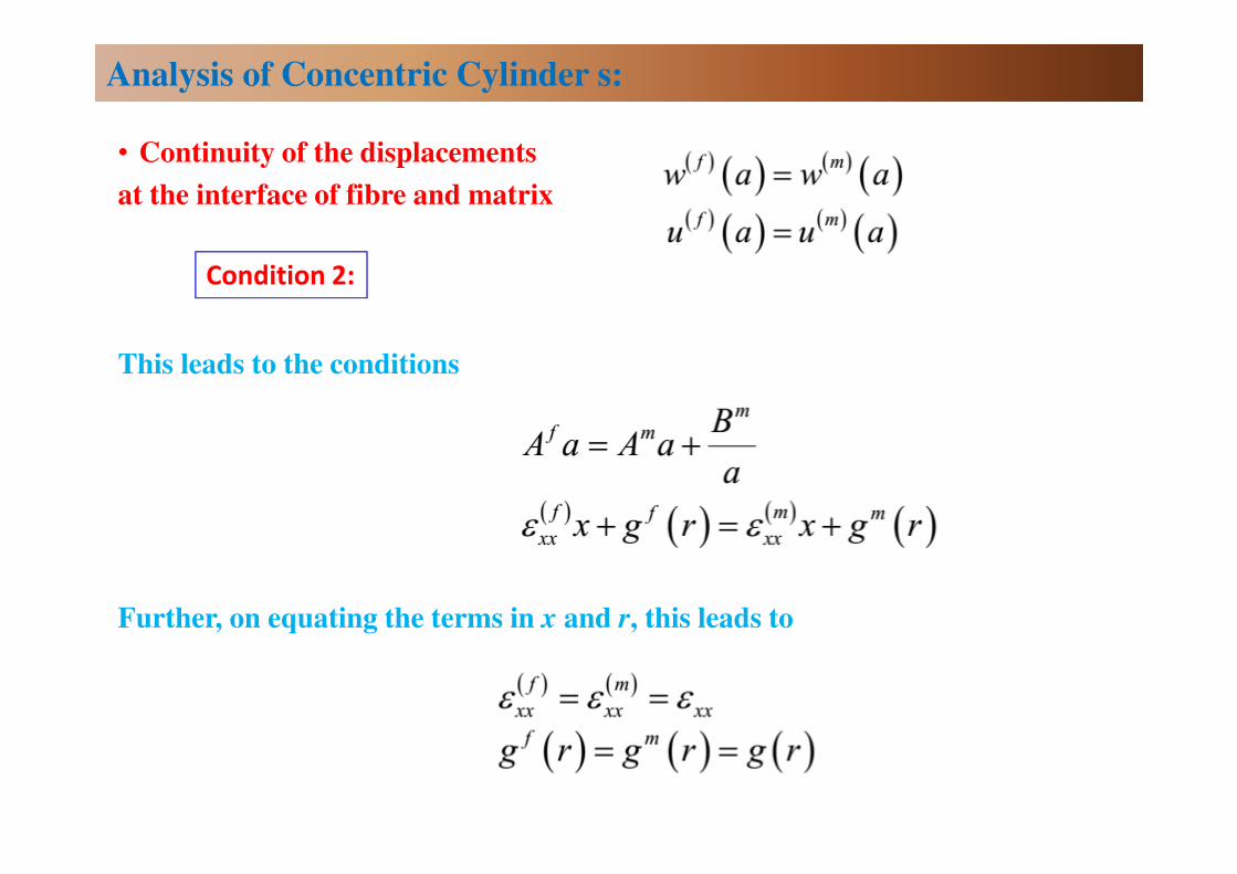
• Continuity of the displacements
at the interface of fibre and matrix
This leads to the conditions
Further, on equating the terms in x and r, this leads to
Analysis of Concentric Cylinder s:
Condition 2:
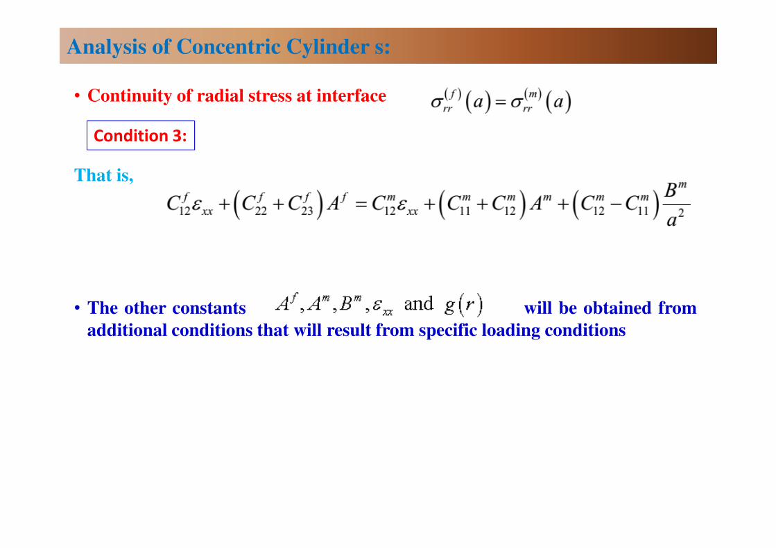
• Continuity of radial stress at interface
That is,
• The other constants will be obtained from
additional conditions that will result from specific loading conditions
Analysis of Concentric Cylinder s:
Condition 3:
Analysis of Concentric Cylinder s:
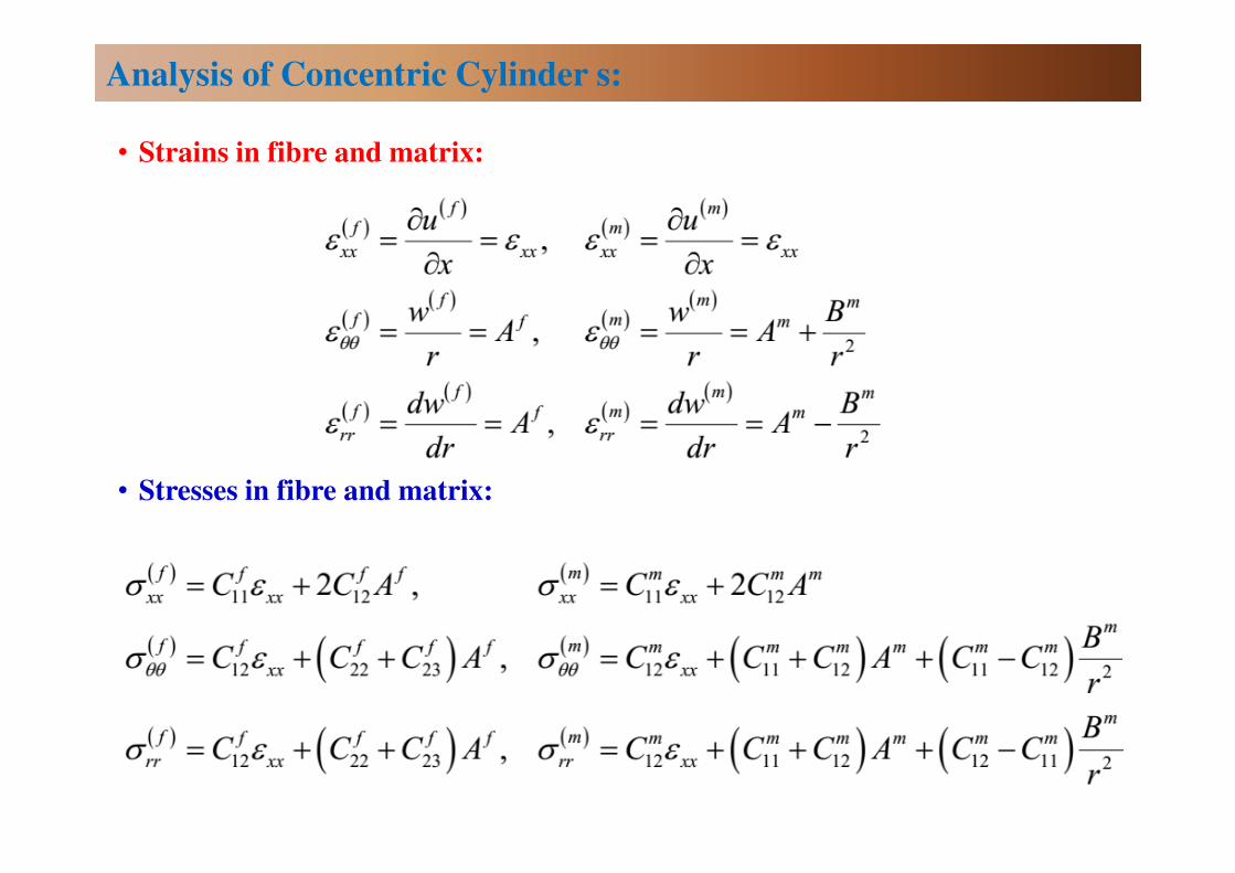
• Strains in fibre and matrix:
• Stresses in fibre and matrix:
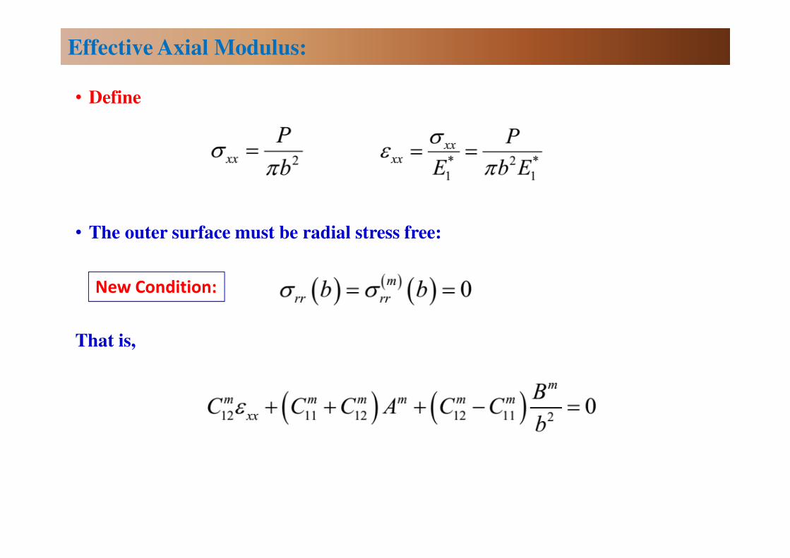
• Define
• The outer surface must be radial stress free:
That is,
Effective Axial Modulus:
New Condition:

Effective Axial Modulus:
• The axial force is obtained as
which gives
Unknowns are solved as
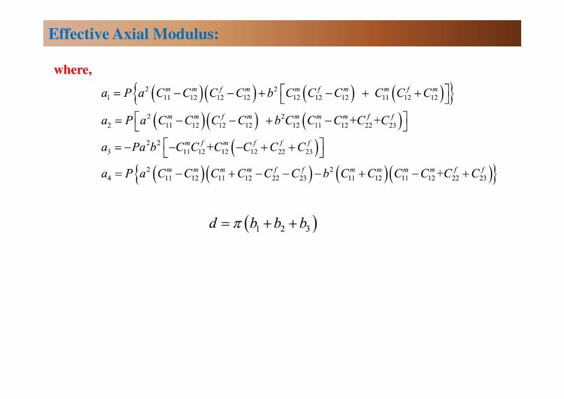
where,
Effective Axial Modulus:
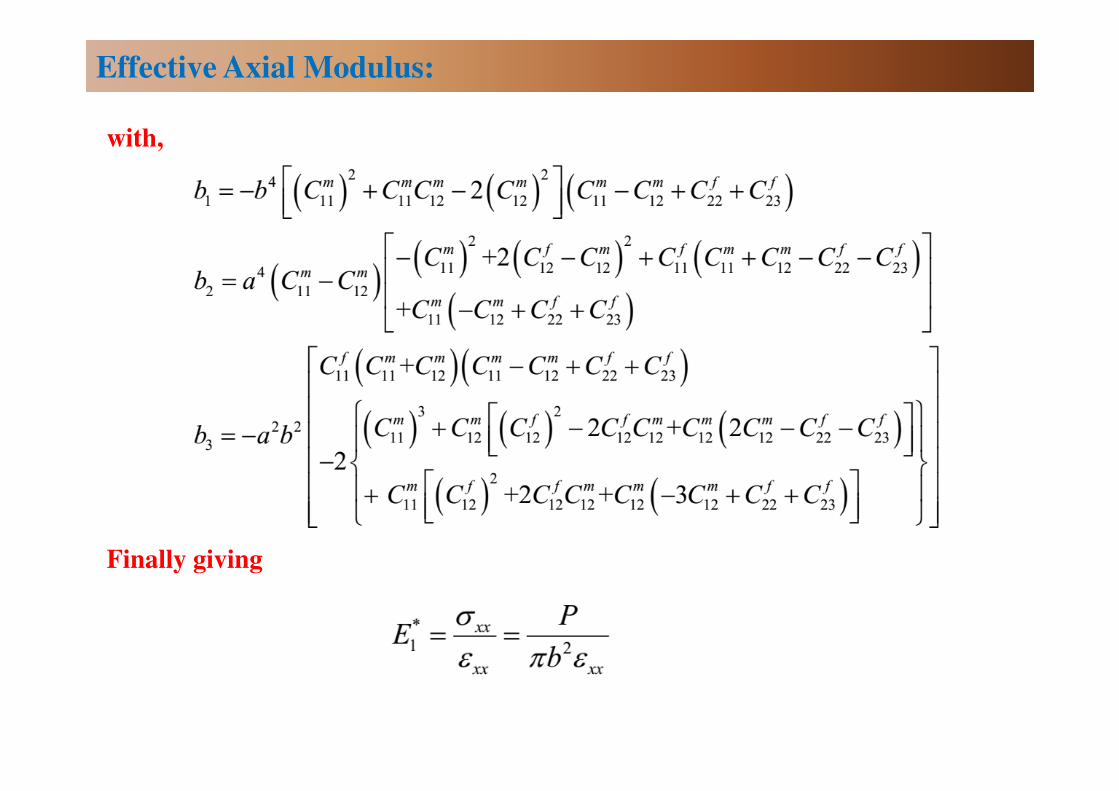
Effective Axial Modulus:
with,
Finally giving
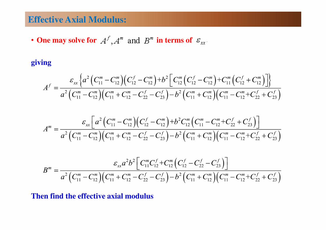
• One may solve for in terms of
giving
Then find the effective axial modulus
Effective Axial Modulus:
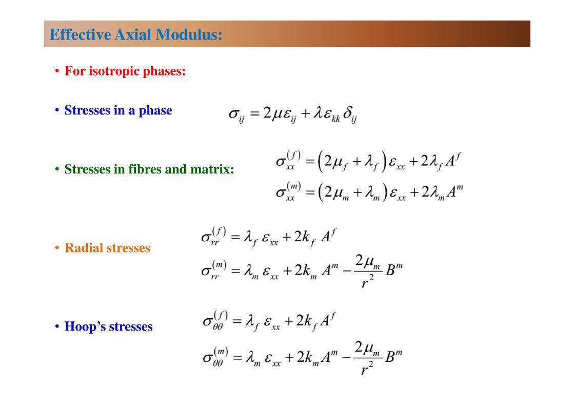
• For isotropic phases:
• Stresses in a phase
• Stresses in fibres and matrix:
• Radial stresses
• Hoop’s stresses
Effective Axial Modulus:
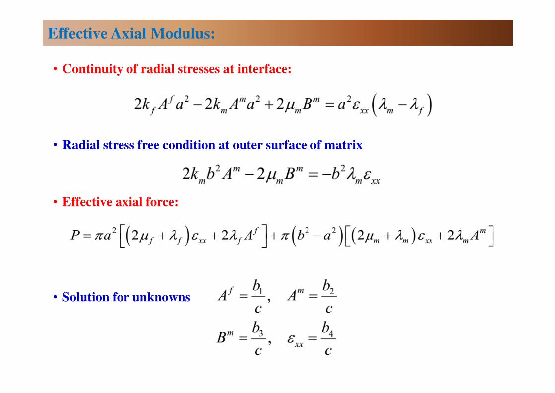
• Continuity of radial stresses at interface:
• Radial stress free condition at outer surface of matrix
• Effective axial force:
• Solution for unknowns
Effective Axial Modulus:
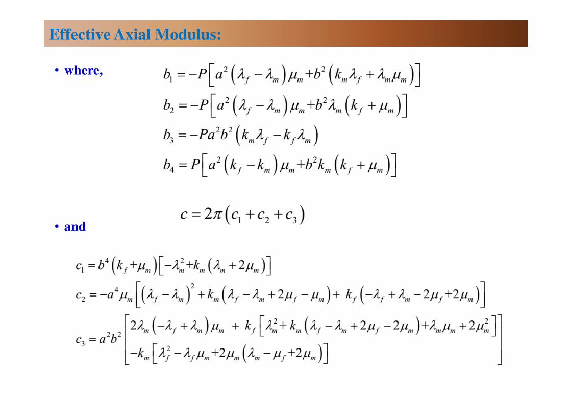
• where,
• and
Effective Axial Modulus:
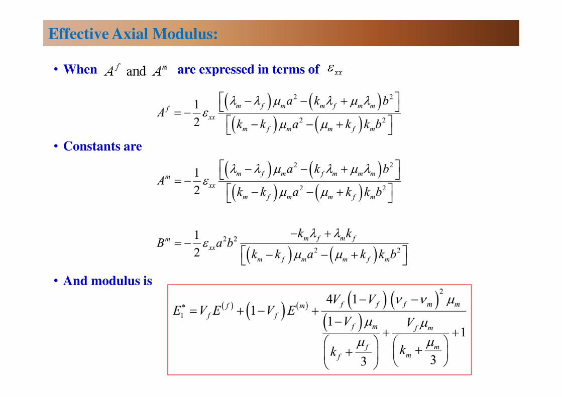
• When are expressed in terms of
• Constants are
• And modulus is
Effective Axial Modulus:
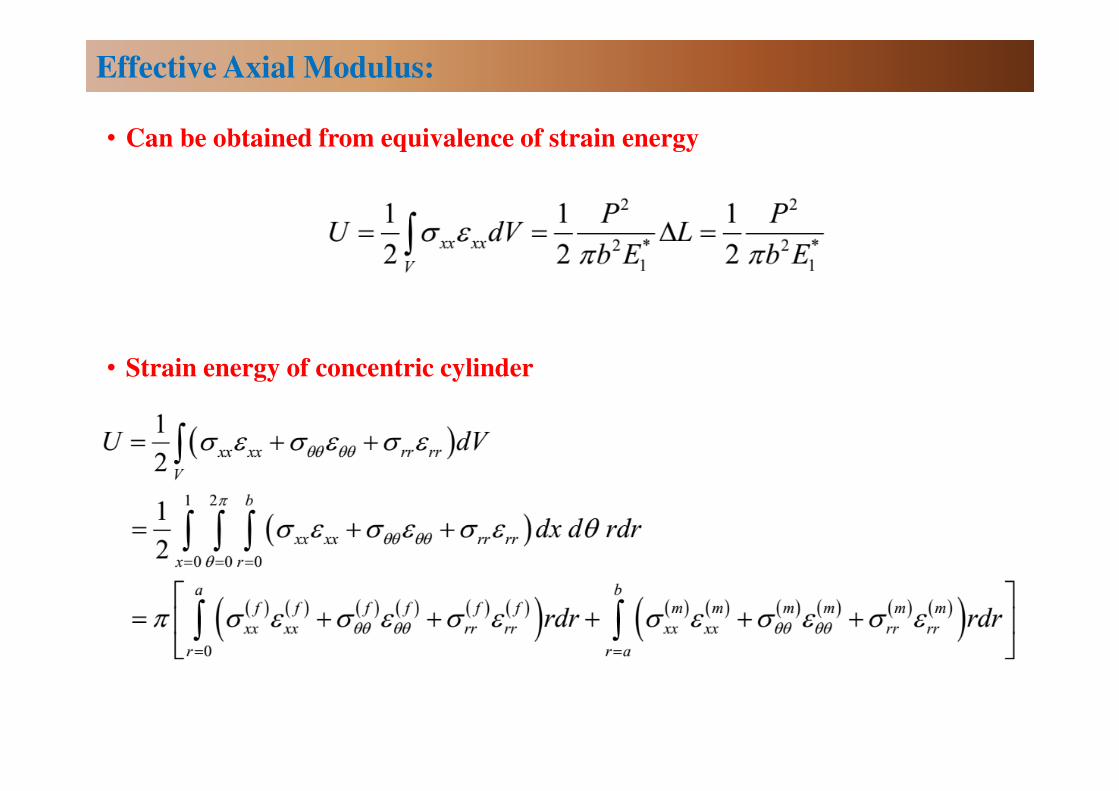
• Can be obtained from equivalence of strain energy
• Strain energy of concentric cylinder
Effective Axial Modulus:
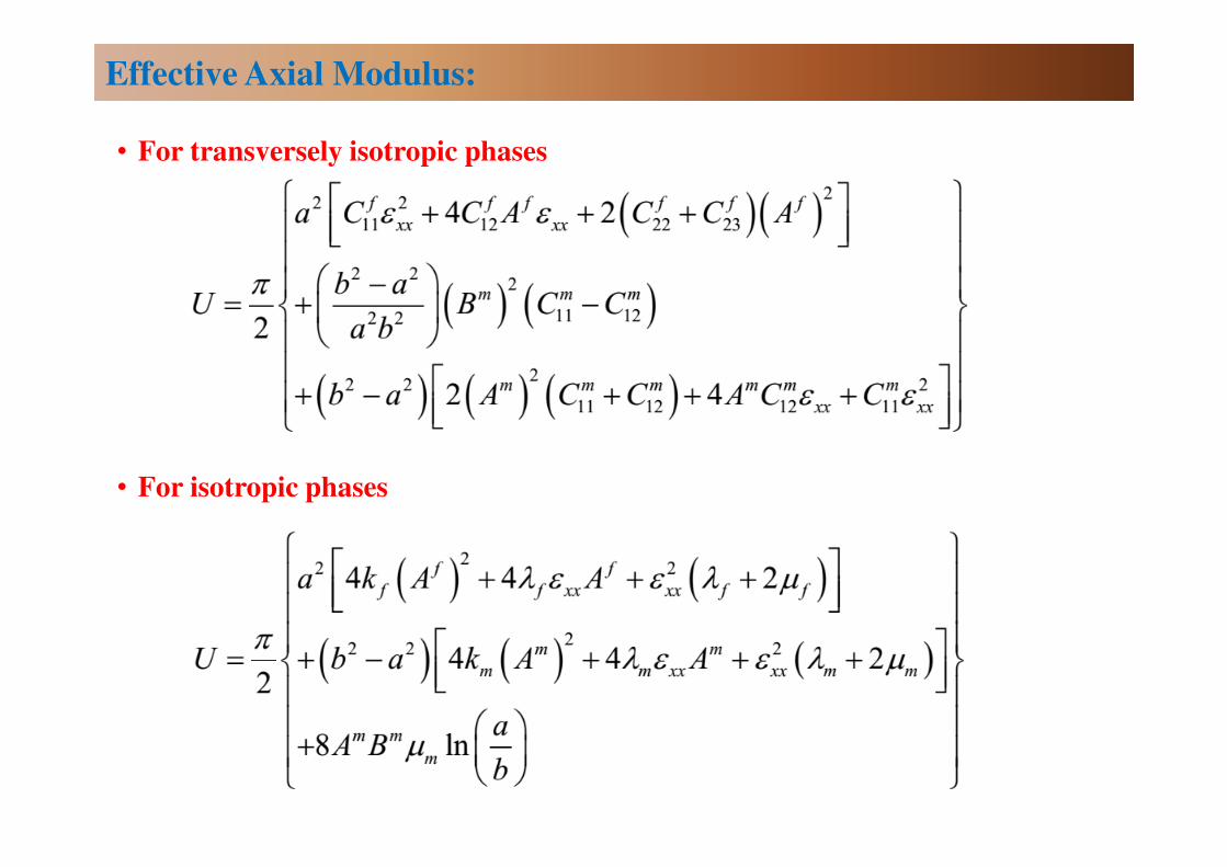
• For transversely isotropic phases
• For isotropic phases
Effective Axial Modulus:
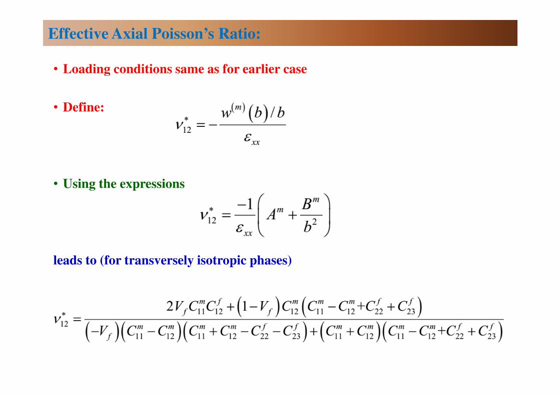
• Loading conditions same as for earlier case
• Define:
• Using the expressions
leads to (for transversely isotropic phases)
Effective Axial Poisson’s Ratio:
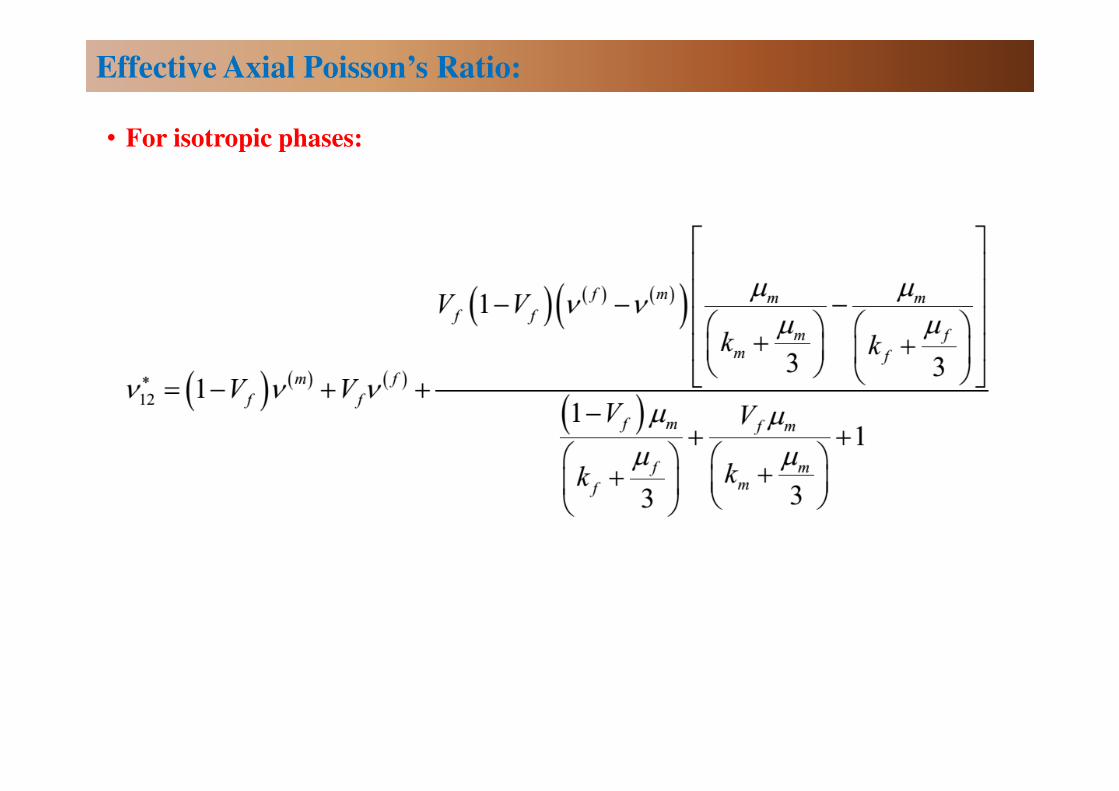
• For isotropic phases:
Effective Axial Poisson’s Ratio:
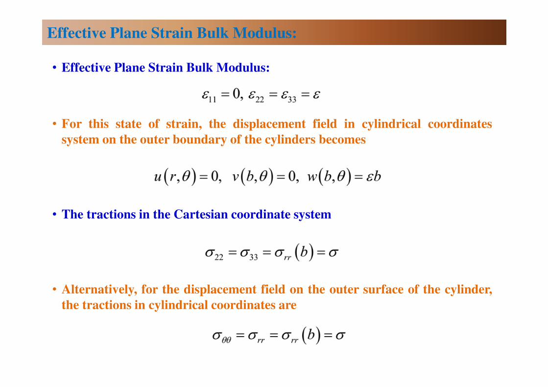
• Effective Plane Strain Bulk Modulus:
• For this state of strain, the displacement field in cylindrical coordinates
system on the outer boundary of the cylinders becomes
• The tractions in the Cartesian coordinate system
• Alternatively, for the displacement field on the outer surface of the cylinder,
the tractions in cylindrical coordinates are
Effective Plane Strain Bulk Modulus:
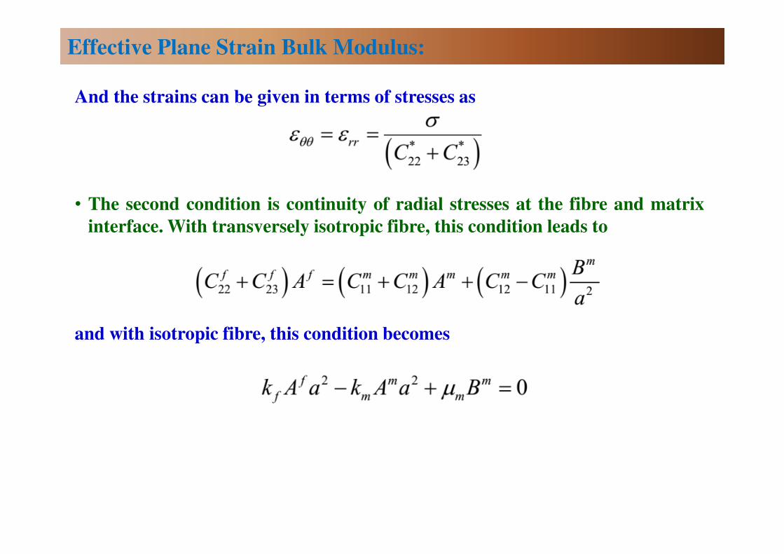
And the strains can be given in terms of stresses as
• The second condition is continuity of radial stresses at the fibre and matrix
interface. With transversely isotropic fibre, this condition leads to
and with isotropic fibre, this condition becomes
Effective Plane Strain Bulk Modulus:
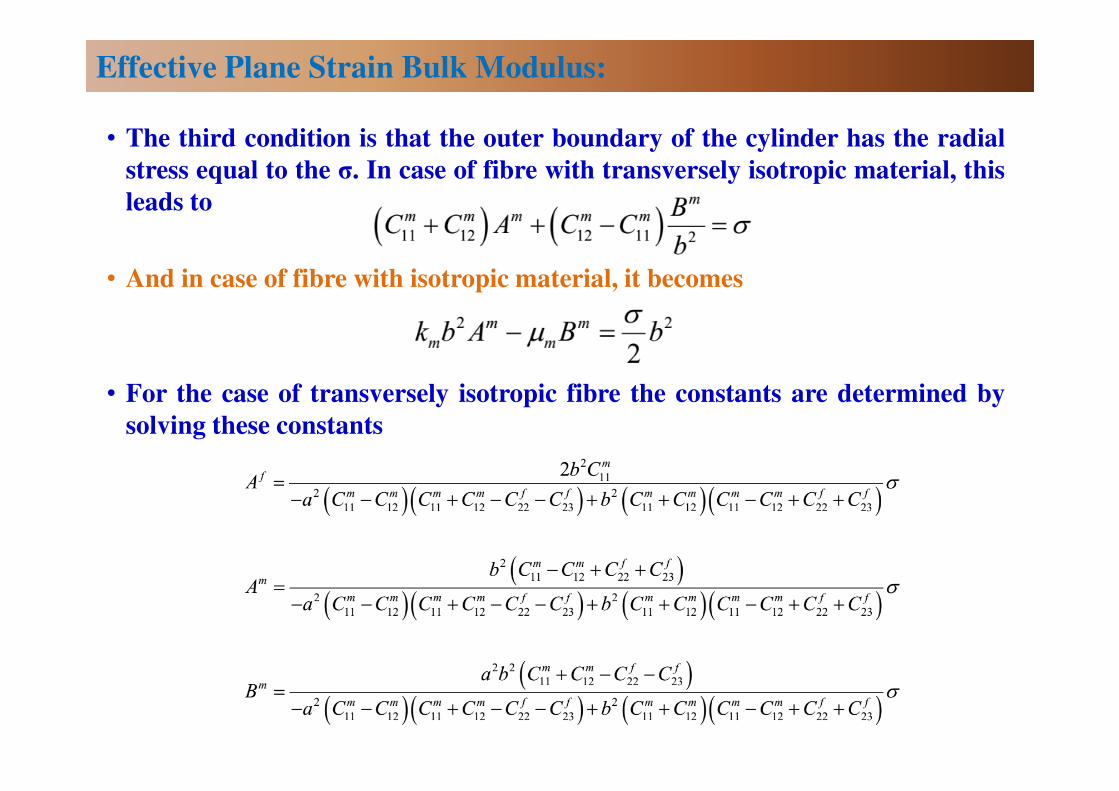
• The third condition is that the outer boundary of the cylinder has the radial
stress equal to the σ. In case of fibre with transversely isotropic material, this
leads to
• And in case of fibre with isotropic material, it becomes
• For the case of transversely isotropic fibre the constants are determined by
solving these constants
Effective Plane Strain Bulk Modulus:
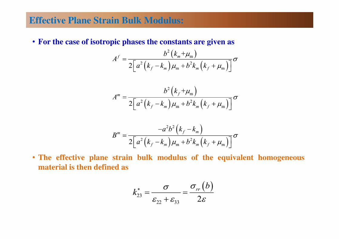
• For the case of isotropic phases the constants are given as
• The effective plane strain bulk modulus of the equivalent homogeneous
material is then defined as
Effective Plane Strain Bulk Modulus:
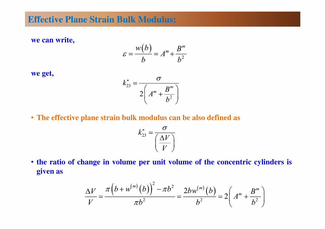
we can write,
we get,
• The effective plane strain bulk modulus can be also defined as
• the ratio of change in volume per unit volume of the concentric cylinders is
given as
Effective Plane Strain Bulk Modulus:
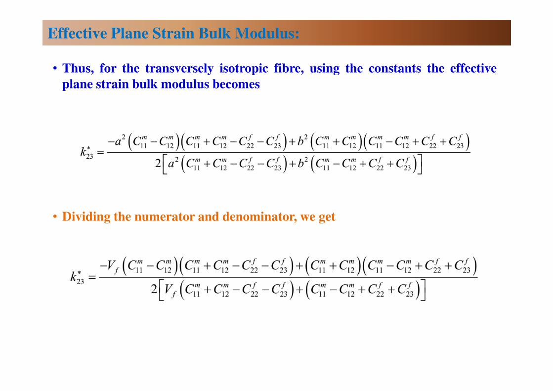
• Thus, for the transversely isotropic fibre, using the constants the effective
plane strain bulk modulus becomes
• Dividing the numerator and denominator, we get
Effective Plane Strain Bulk Modulus:
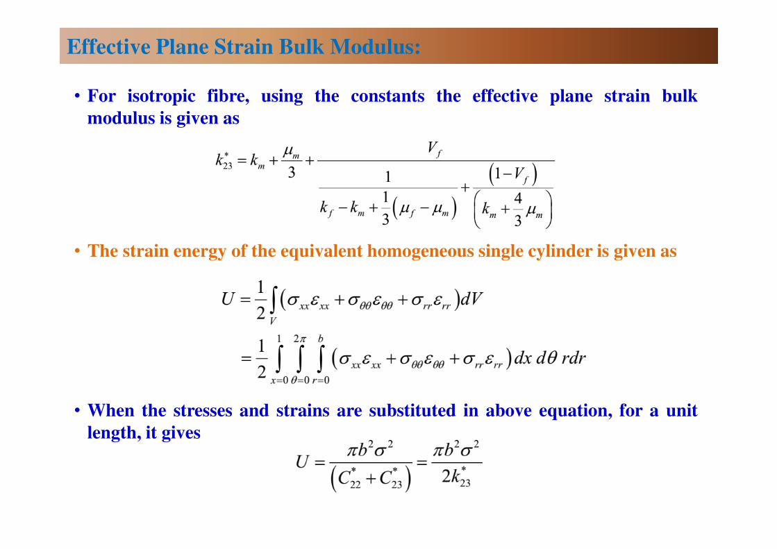
• For isotropic fibre, using the constants the effective plane strain bulk
modulus is given as
• The strain energy of the equivalent homogeneous single cylinder is given as
• When the stresses and strains are substituted in above equation, for a unit
length, it gives
Effective Plane Strain Bulk Modulus:
Effective Axial Shear Modulus:
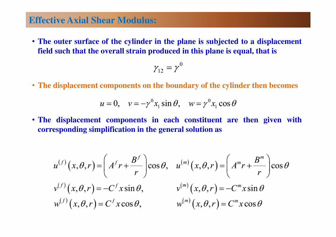
• The outer surface of the cylinder in the plane is subjected to a displacement
field such that the overall strain produced in this plane is equal, that is
• The displacement components on the boundary of the cylinder then becomes
• The displacement components in each constituent are then given with
corresponding simplification in the general solution as
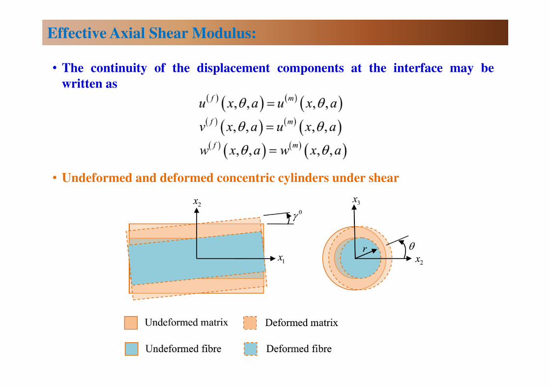
• The continuity of the displacement components at the interface may be
written as
• Undeformed and deformed concentric cylinders under shear
Effective Axial Shear Modulus:

• The first continuity condition (radial displacement) of the above equation
gives the relation
• The remaining two displacement continuity conditions give
• The non-zero stresses resulting from the displacement field
Effective Axial Shear Modulus:

• The continuity of the stresses in radial direction leads the continuity of the
stress at the interface and this condition becomes
• Now, at the outer boundary of the concentric cylinders the displacements
must match the following boundary conditions.
• Note that from the second and the third of the above condition, we get
Effective Axial Shear Modulus:
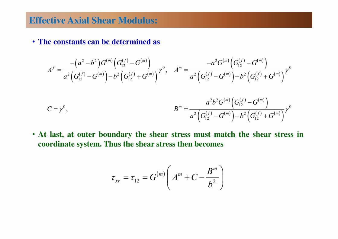
• The constants can be determined as
• At last, at outer boundary the shear stress must match the shear stress in
coordinate system. Thus the shear stress then becomes
Effective Axial Shear Modulus:
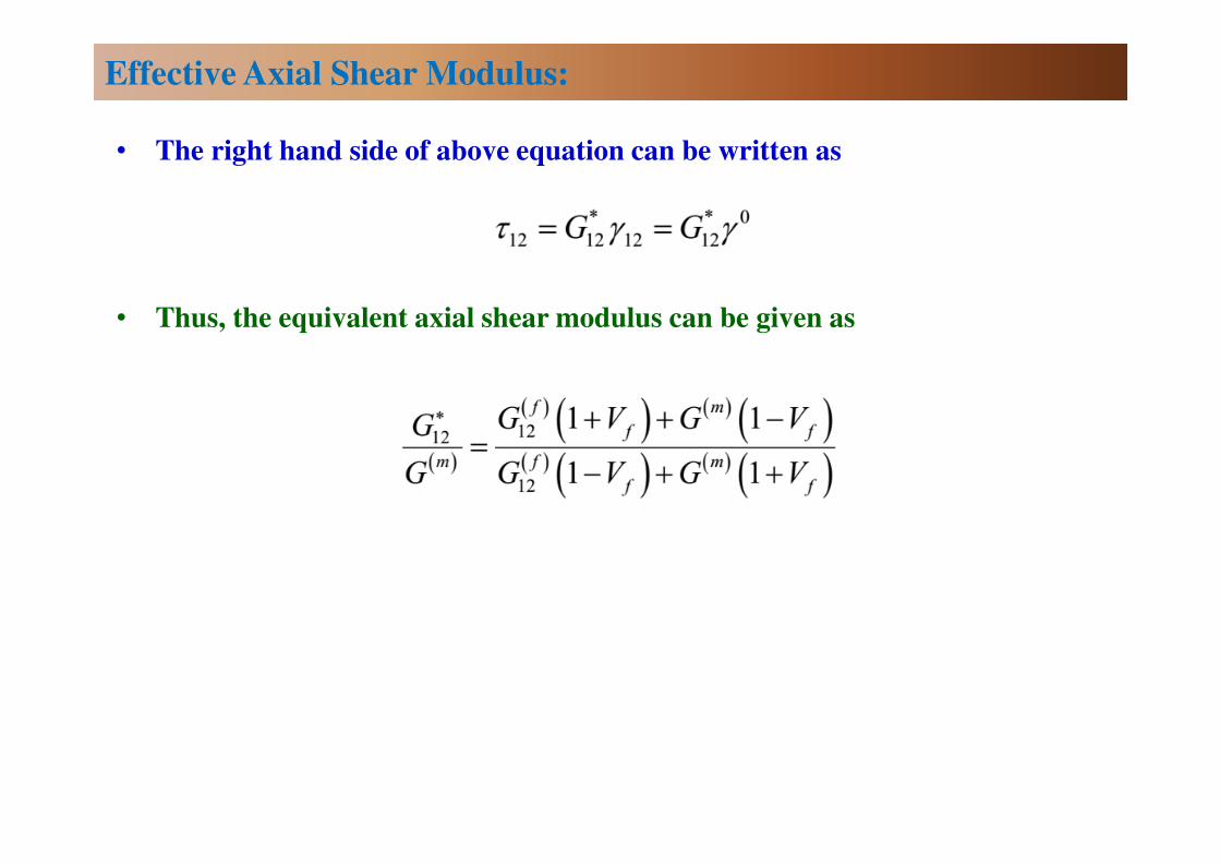
• The right hand side of above equation can be written as
• Thus, the equivalent axial shear modulus can be given as
Effective Axial Shear Modulus:
Three Phase Concentric Cylinder
Assemblage Model
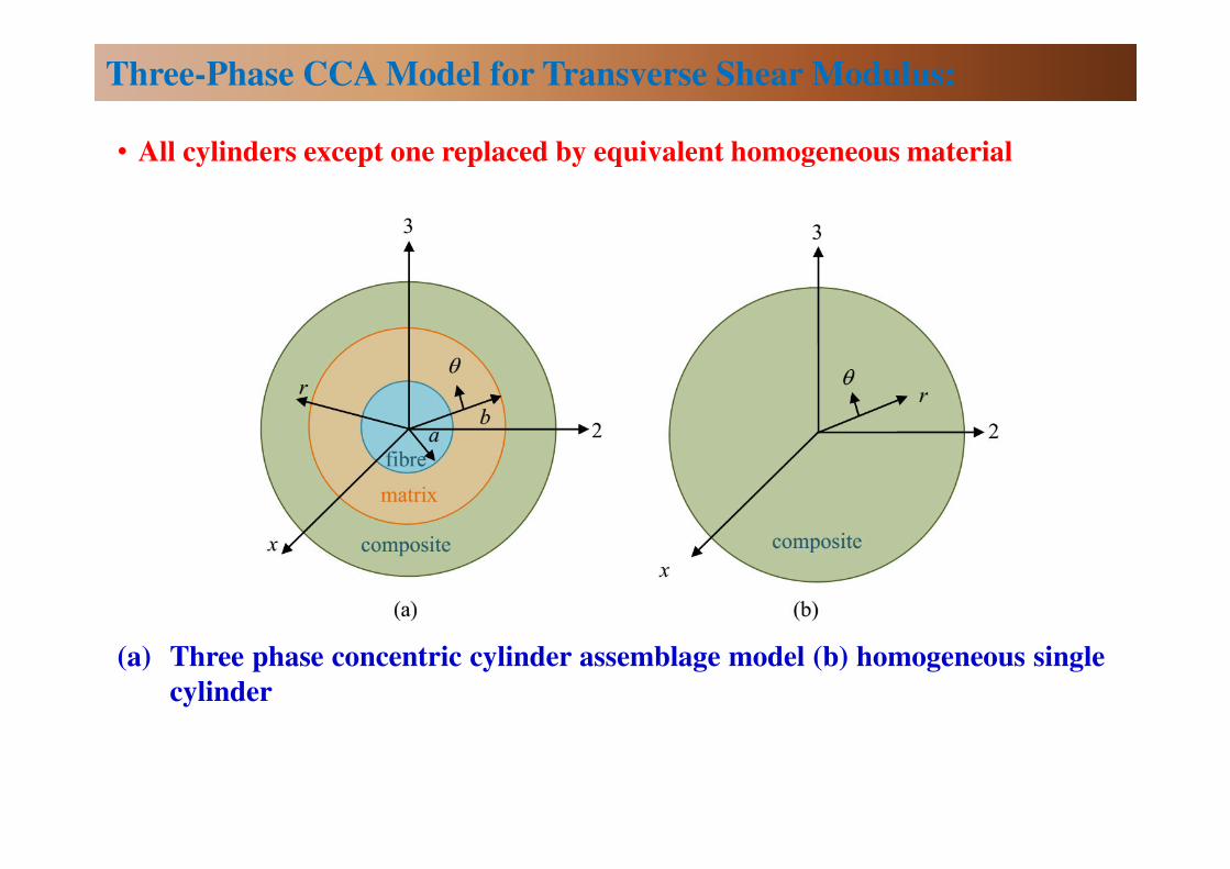
• All cylinders except one replaced by equivalent homogeneous material
(a) Three phase concentric cylinder assemblage model (b) homogeneous single
cylinder
Three-Phase CCA Model for Transverse Shear Modulus:
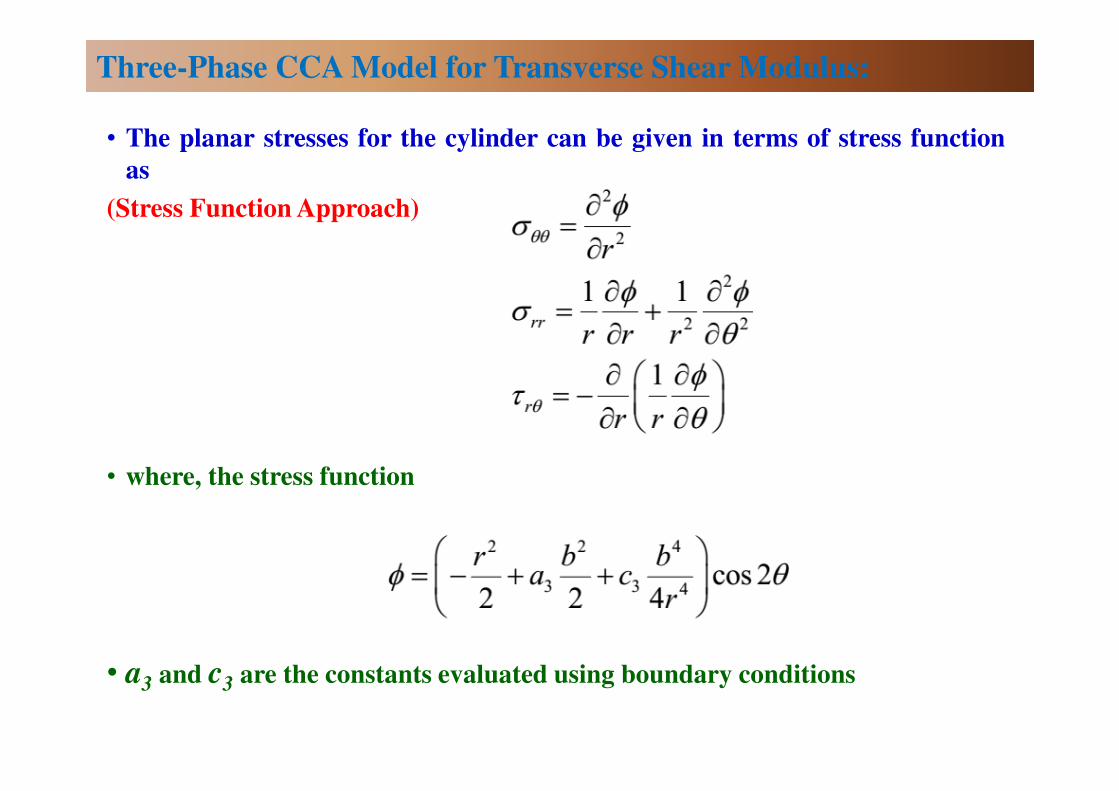
• The planar stresses for the cylinder can be given in terms of stress function
as
(Stress Function Approach)
• where, the stress function
• a3 and c3 are the constants evaluated using boundary conditions
Three-Phase CCA Model for Transverse Shear Modulus:
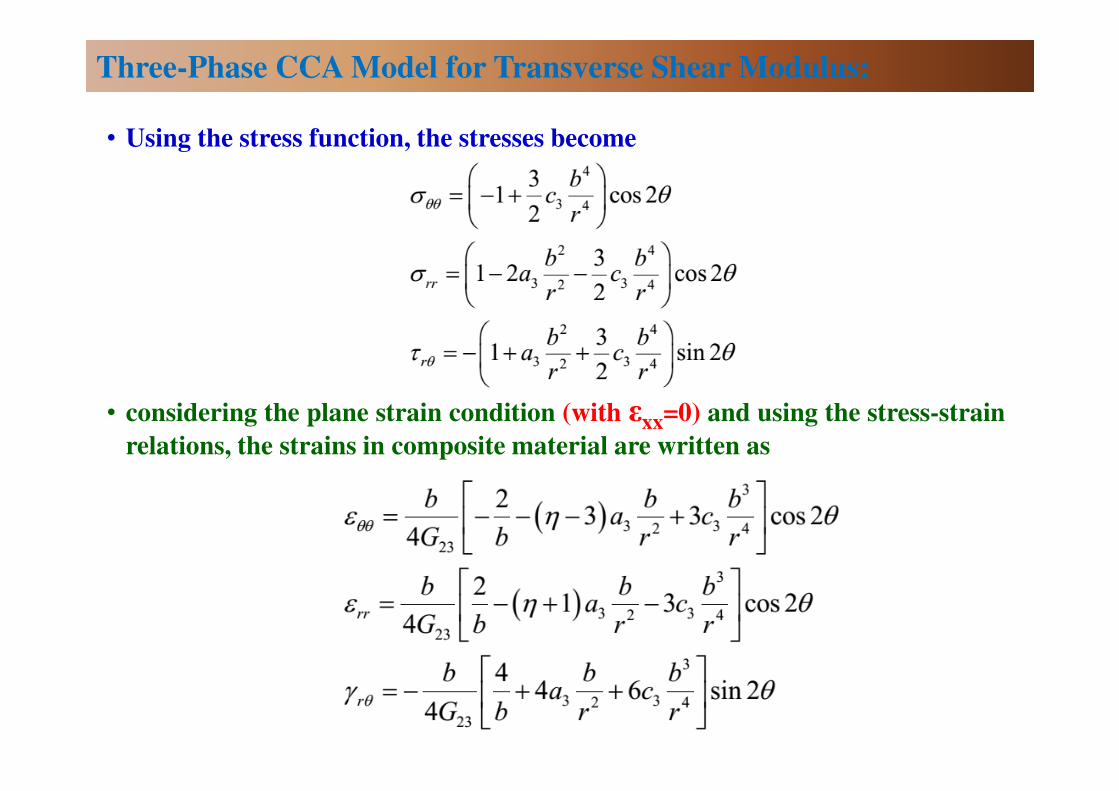
• Using the stress function, the stresses become
• considering the plane strain condition (with εxx=0) and using the stress-strain
relations, the strains in composite material are written as
Three-Phase CCA Model for Transverse Shear Modulus:
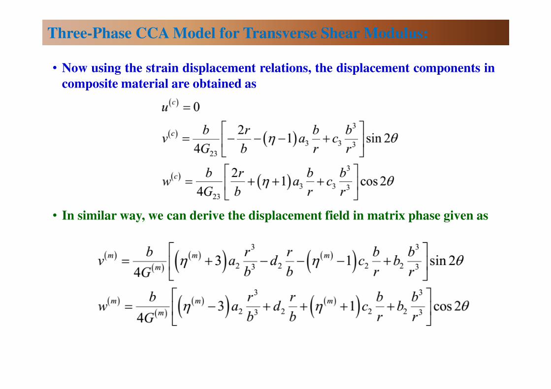
• Now using the strain displacement relations, the displacement components in
composite material are obtained as
• In similar way, we can derive the displacement field in matrix phase given as
Three-Phase CCA Model for Transverse Shear Modulus:
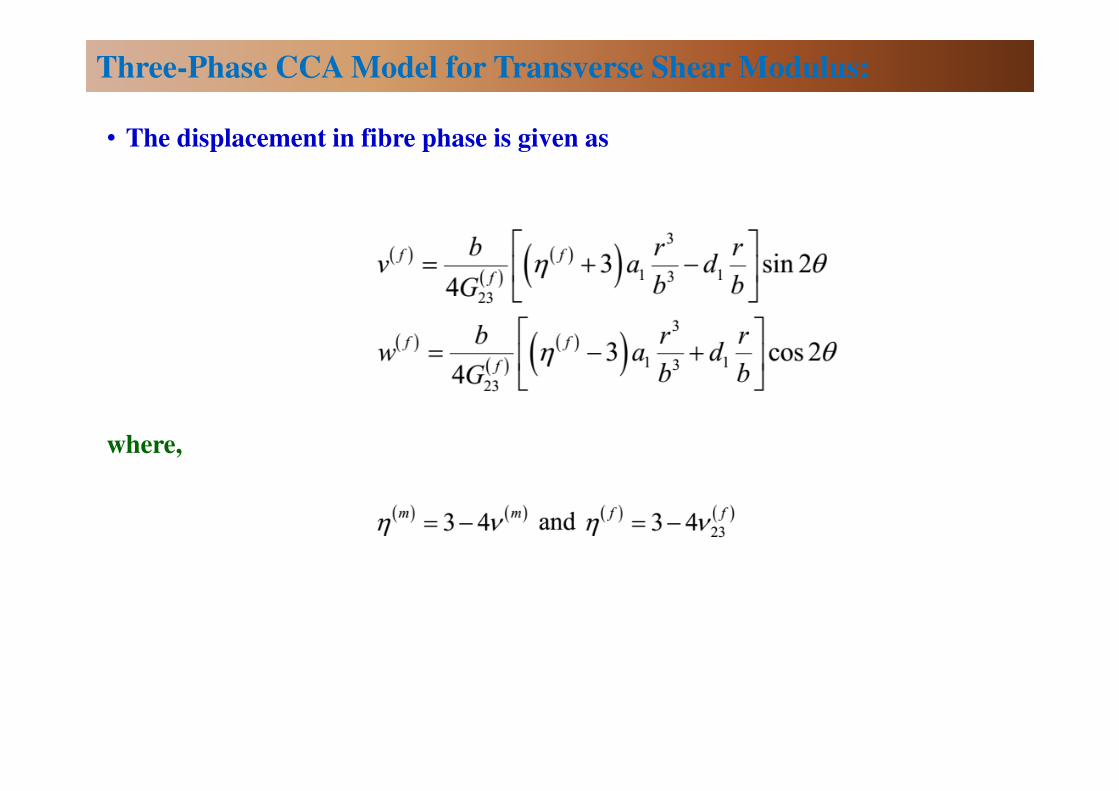
• The displacement in fibre phase is given as
where,
Three-Phase CCA Model for Transverse Shear Modulus:

• The displacement continuity at r = a gives the relations
• The displacement continuity at r = b gives
Three-Phase CCA Model for Transverse Shear Modulus:
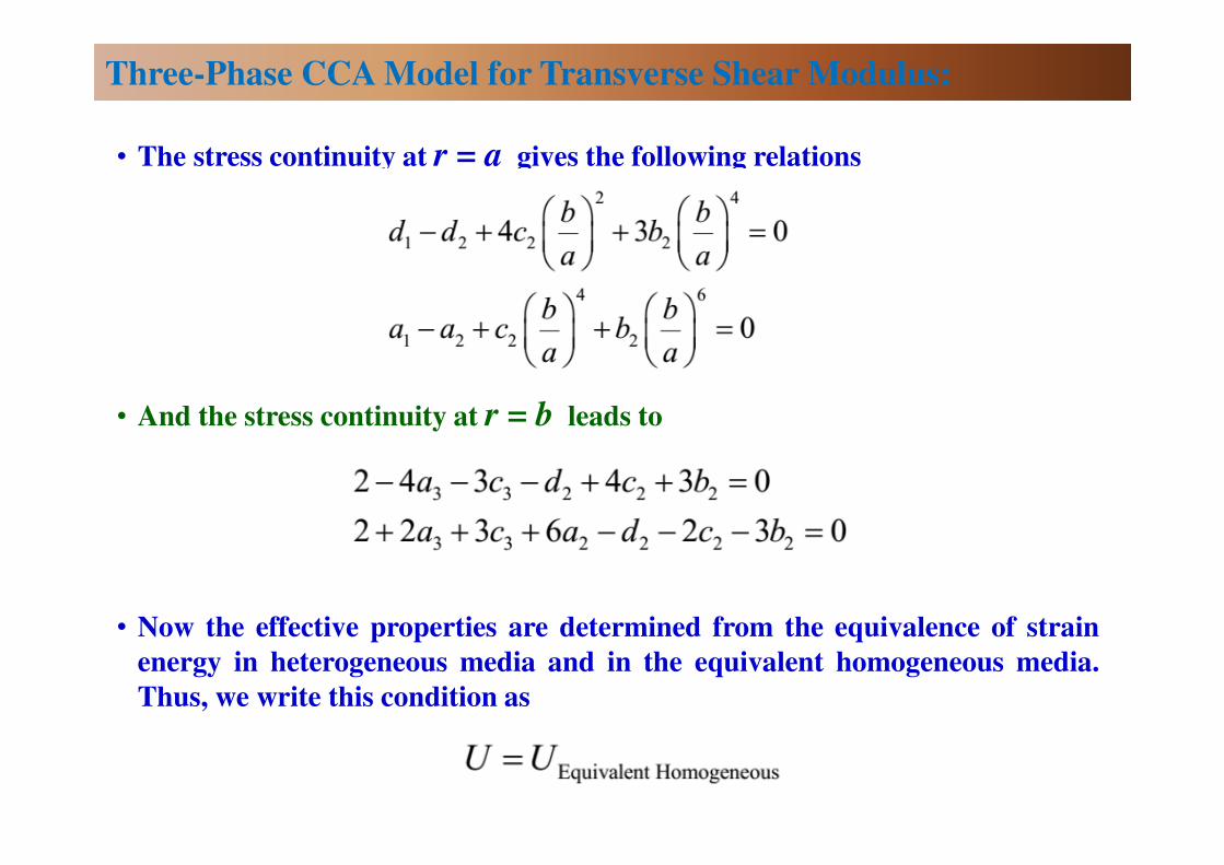
• The stress continuity at r = a gives the following relations
• And the stress continuity at r = b leads to
• Now the effective properties are determined from the equivalence of strain
energy in heterogeneous media and in the equivalent homogeneous media.
Thus, we write this condition as
Three-Phase CCA Model for Transverse Shear Modulus:
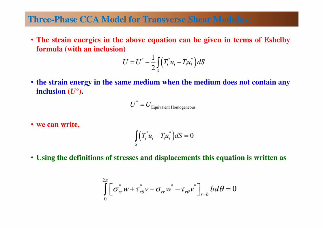
• The strain energies in the above equation can be given in terms of Eshelby
formula (with an inclusion)
• the strain energy in the same medium when the medium does not contain any
inclusion (U°).
• we can write,
• Using the definitions of stresses and displacements this equation is written as
Three-Phase CCA Model for Transverse Shear Modulus:
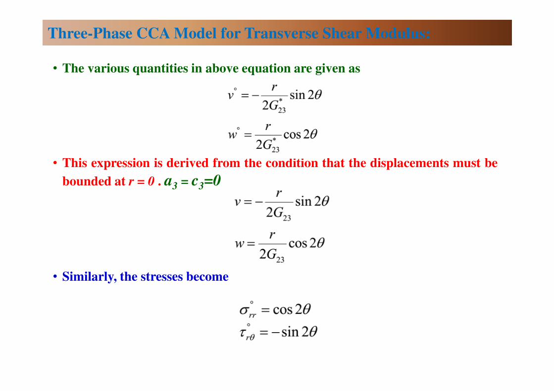
• The various quantities in above equation are given as
• This expression is derived from the condition that the displacements must be
bounded at r = 0 . a3 = c3=0
• Similarly, the stresses become
Three-Phase CCA Model for Transverse Shear Modulus:
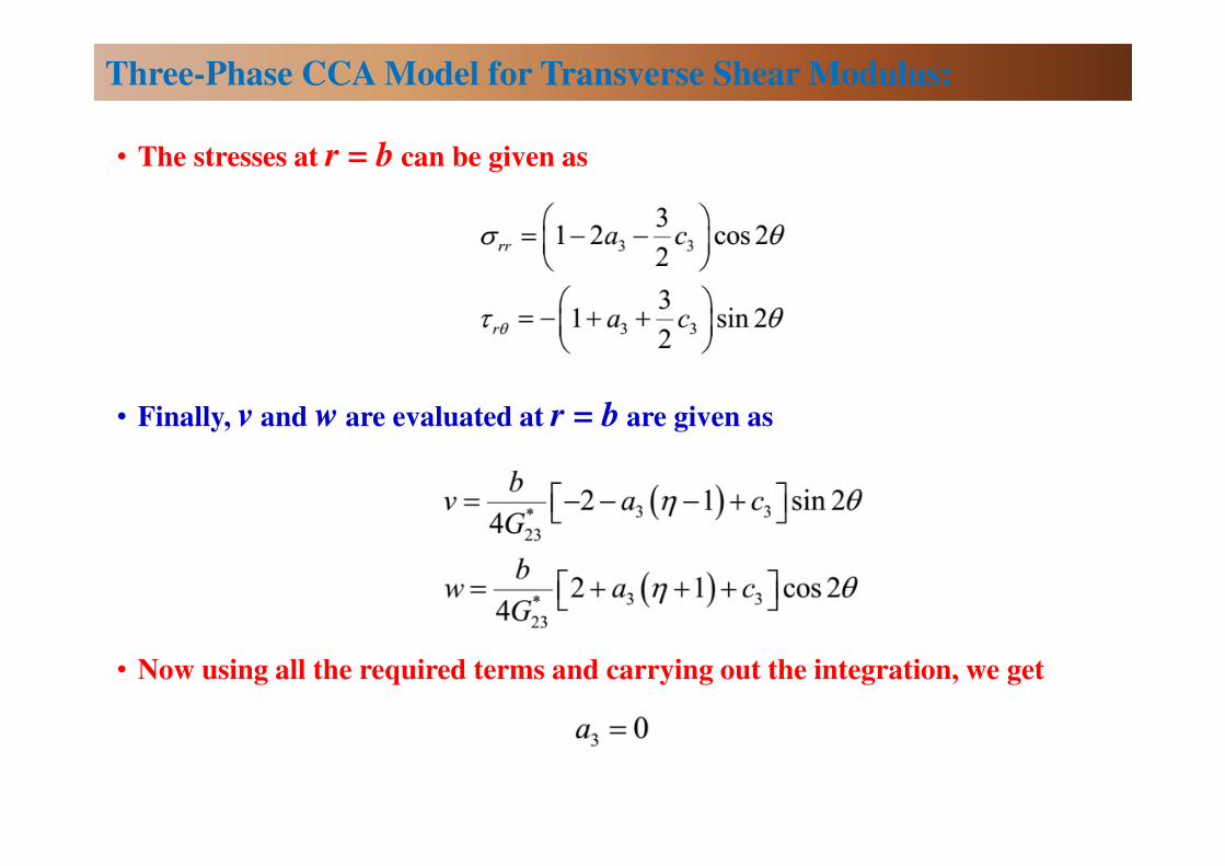
• The stresses at r = b can be given as
• Finally, v and w are evaluated at r = b are given as
• Now using all the required terms and carrying out the integration, we get
Three-Phase CCA Model for Transverse Shear Modulus:
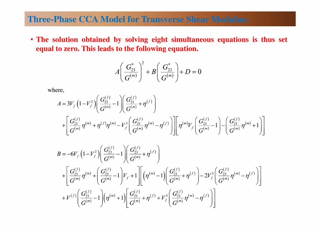
• The solution obtained by solving eight simultaneous equations is thus set
equal to zero. This leads to the following equation.
Three-Phase CCA Model for Transverse Shear Modulus:
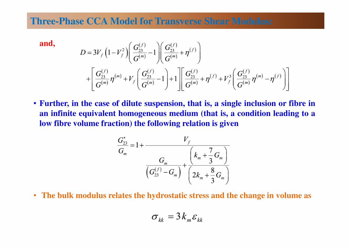
and,
• Further, in the case of dilute suspension, that is, a single inclusion or fibre in
an infinite equivalent homogeneous medium (that is, a condition leading to a
low fibre volume fraction) the following relation is given
• The bulk modulus relates the hydrostatic stress and the change in volume as
Three-Phase CCA Model for Transverse Shear Modulus:
Self Consistent Method
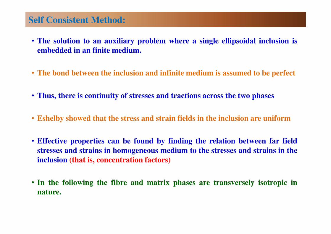
• The solution to an auxiliary problem where a single ellipsoidal inclusion is
embedded in an finite medium.
• The bond between the inclusion and infinite medium is assumed to be perfect
• Thus, there is continuity of stresses and tractions across the two phases
• Eshelby showed that the stress and strain fields in the inclusion are uniform
• Effective properties can be found by finding the relation between far field
stresses and strains in homogeneous medium to the stresses and strains in the
inclusion (that is, concentration factors)
• In the following the fibre and matrix phases are transversely isotropic in
nature.
Self Consistent Method:
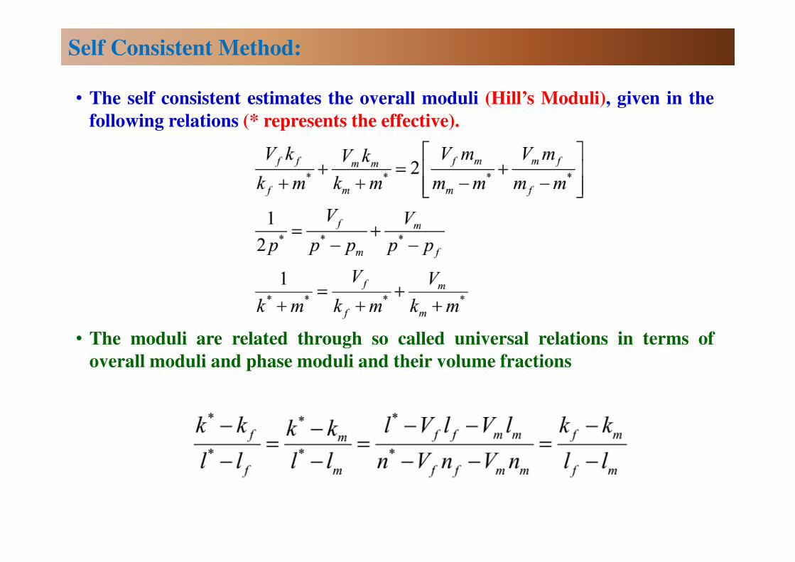
• The self consistent estimates the overall moduli (Hill’s Moduli), given in the
following relations (* represents the effective).
• The moduli are related through so called universal relations in terms of
overall moduli and phase moduli and their volume fractions
Self Consistent Method:
Mori Tanaka Method
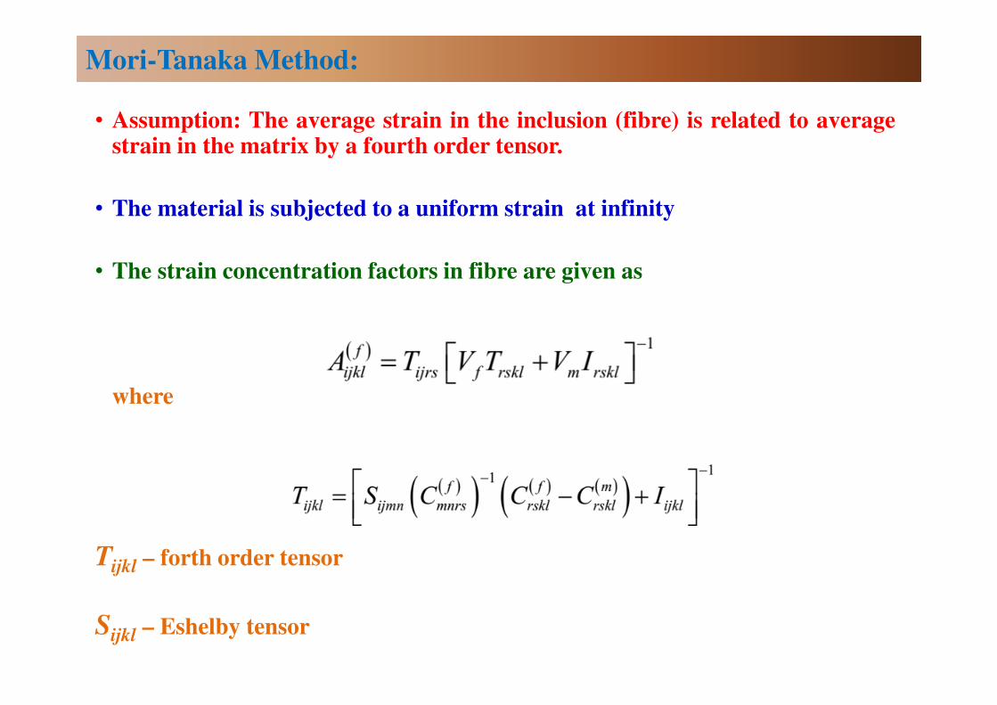
• Assumption: The average strain in the inclusion (fibre) is related to averagestrain in the matrix by a fourth order tensor.
• The material is subjected to a uniform strain at infinity
• The strain concentration factors in fibre are given as
where
Tijkl – forth order tensor
Sijkl – Eshelby tensor
Mori-Tanaka Method:
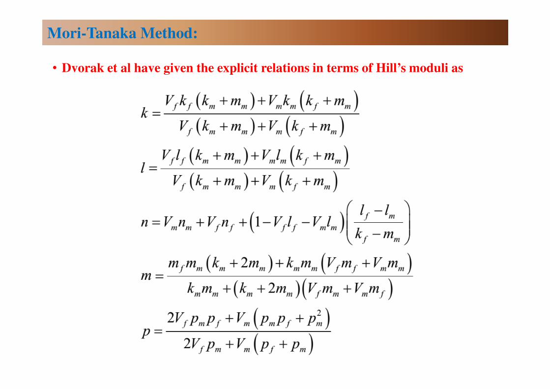
• Dvorak et al have given the explicit relations in terms of Hill’s moduli as
Mori-Tanaka Method:

• In case of transversely isotropic material in 23 plane, the constitutive
relations are given as
and
Hill’s Moduli:
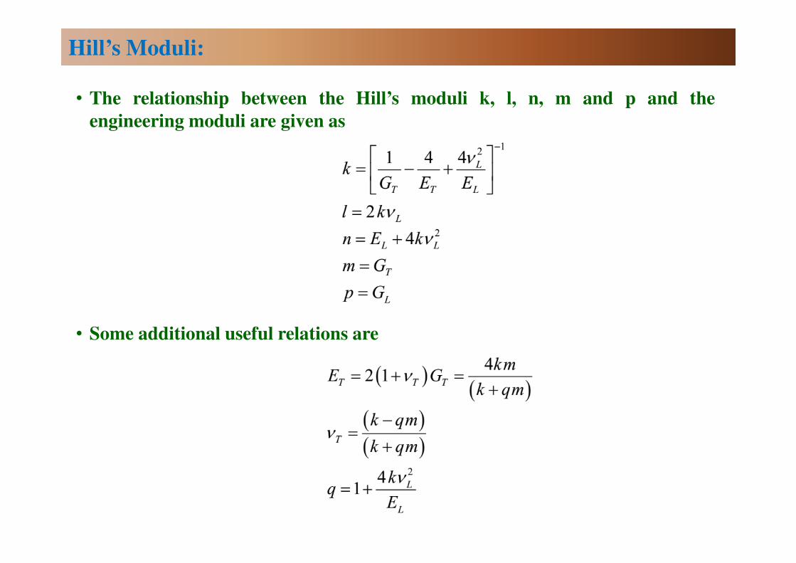
• The relationship between the Hill’s moduli k, l, n, m and p and the
engineering moduli are given as
• Some additional useful relations are
Hill’s Moduli:
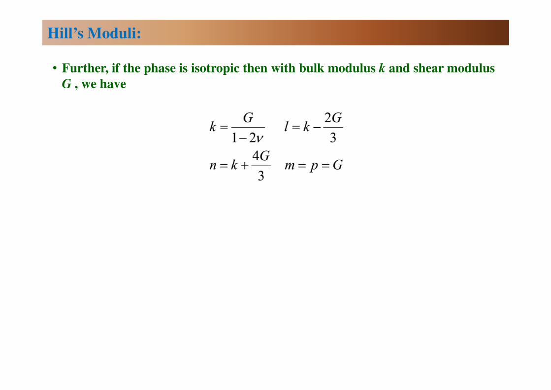
• Further, if the phase is isotropic then with bulk modulus k and shear modulus
G , we have
Hill’s Moduli:
Halpin Tsai Models
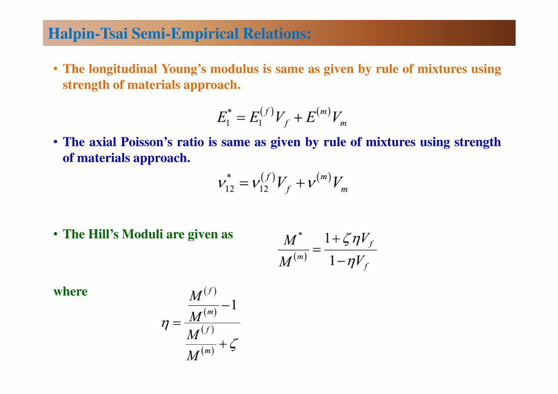
• The longitudinal Young’s modulus is same as given by rule of mixtures using
strength of materials approach.
• The axial Poisson’s ratio is same as given by rule of mixtures using strength
of materials approach.
• The Hill’s Moduli are given as
where
Halpin-Tsai Semi-Empirical Relations:
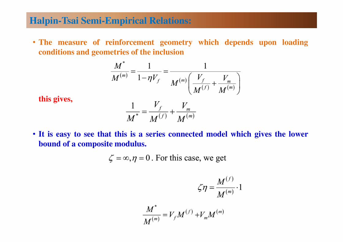
• The measure of reinforcement geometry which depends upon loading
conditions and geometries of the inclusion
this gives,
• It is easy to see that this is a series connected model which gives the lower
bound of a composite modulus.
Halpin-Tsai Semi-Empirical Relations:

Hashin Shtrikman Bounds
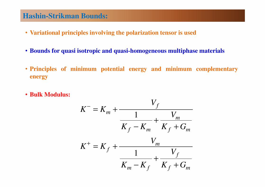
• Variational principles involving the polarization tensor is used
• Bounds for quasi isotropic and quasi-homogeneous multiphase materials
• Principles of minimum potential energy and minimum complementary
energy
• Bulk Modulus:
Hashin-Strikman Bounds:
1
1
f
mm
f m f m
mf
f
m f f m
VK K
V
K K K G
VK K
V
K K K G
−
+
= +
+− +
= +
+− +
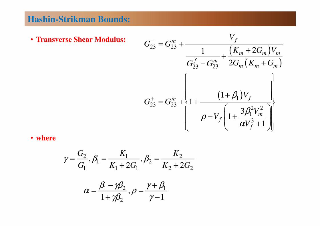
• Transverse Shear Modulus:
• where
Hashin-Strikman Bounds:
( )( )
( )
23 23
2323
1
23 232 2
1
3
21
2
11
31
1
fm
m m m
f mm m m
fm
mf
f
VG G
K G V
G K GG G
VG G
VV
V
β
βρ
α
−
+
= ++
++−
+
= + + − + +
2 1 21 2
1 1 1 2 2
, ,2 2
G K K
G K G K Gγ β β= = =
+ +
1 2 1
2
,1 1
β γβ γ βα ρ
γβ γ
− += =
+ −
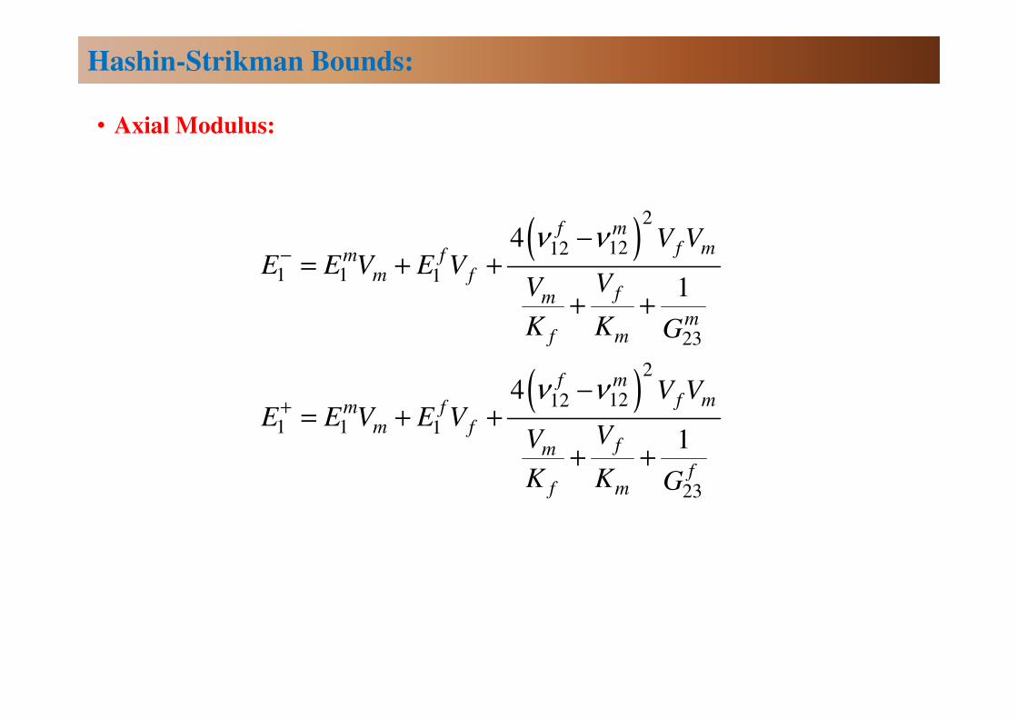
• Axial Modulus:
Hashin-Strikman Bounds:
( )
( )
2
1212
1 1 1
23
2
1212
1 1 1
23
4
1
4
1
f mf mfm
m ffm
mf m
f mf mfm
m ffm
ff m
V VE E V E V
VV
K K G
V VE E V E V
VV
K K G
ν ν
ν ν
−
+
−= + +
+ +
−= + +
+ +
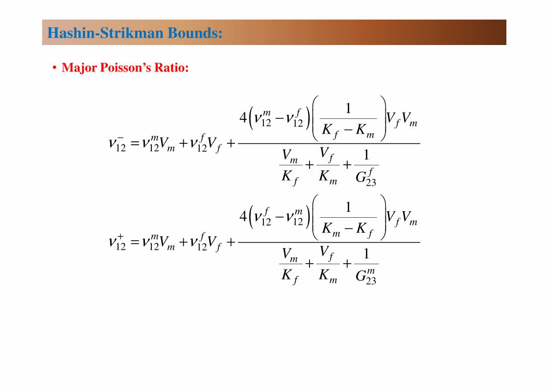
• Major Poisson’s Ratio:
Hashin-Strikman Bounds:
( )
( )
12 12
12 12 12
23
1212
12 12 12
23
14
1
14
1
fmf m
f mfmm f
fmf
f m
f mf m
m ffmm f
fmm
f m
V VK K
V VVV
K K G
V VK K
V VVV
K K G
ν ν
ν ν ν
ν ν
ν ν ν
−
+
−
− = + +
+ +
−
− = + +
+ +
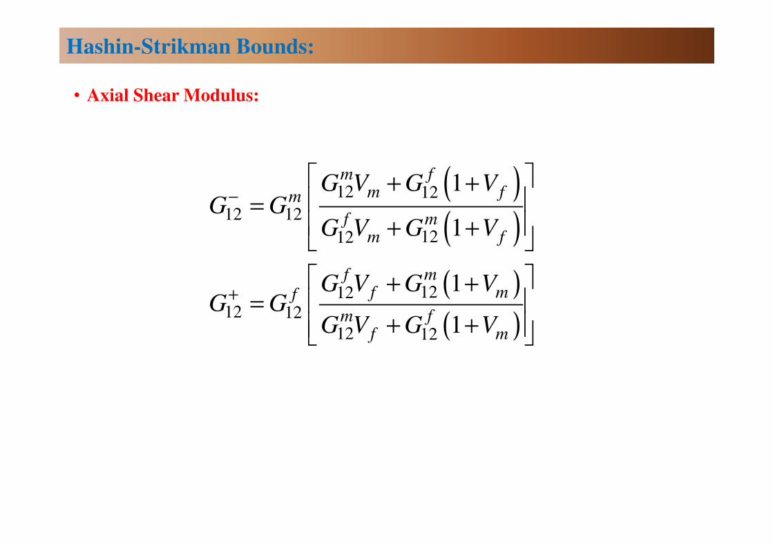
• Axial Shear Modulus:
Hashin-Strikman Bounds:
( )( )
( )
( )
12 12
12 12
1212
1212
12 12
12 12
1
1
1
1
fmm fm
f mm f
f mf mf
fmf m
G V G VG G
G V G V
G V G VG G
G V G V
−
+
+ + = + +
+ + =
+ +

Thank You


![A Review on Natural Fibre Reinforced Polymer Composites · natural fibre reinforced polymer composites increase with increasing fibre loading. Khoathane et al. [1] found that the](https://static.fdocuments.net/doc/165x107/5e21837fc2d50e18910e61ca/a-review-on-natural-fibre-reinforced-polymer-composites-natural-fibre-reinforced.jpg)


![Azoti, Wiyao and Elmarakbi, Ahmed (2016) Micromechanics ...sure.sunderland.ac.uk/9227/1/4. ASME.pdfmechanics in particle and fibre-reinforced composites [8]. Then, the accuracy of](https://static.fdocuments.net/doc/165x107/6123e666f770d113196f6486/azoti-wiyao-and-elmarakbi-ahmed-2016-micromechanics-sure-asmepdf-mechanics.jpg)
