The CAPM, National Stock Market Betas, and Macroeconomic Covariates: A Global Analysis.

Michael Curran, Villanova University

Adnan Velic, Dublin Institute of Technology

TEP Working Paper No. 0618

August 2018

Trinity Economics Papers Department of Economics

The CAPM, National Stock Market Betas, andMacroeconomic Covariates: A Global Analysis∗

Michael Curran†

Villanova University

Adnan Velic‡

Dublin Institute of Technology

August 3, 2018

Abstract

Using global data on aggregate stock market prices, this paper finds that the stan-

dard capital asset pricing model (CAPM) fares much better than suggested in the

literature. At shorter time horizons, our results also show that the positive risk-reward

relation can collapse during times of high volatility. Compared to advanced and emerg-

ing markets, we retrieve evidence of lower systematic risks across frontier stock market

portfolios. We find that countries characterized by higher levels of financial and trade

openness, exchange rate volatility, and larger economic size are exposed to higher sys-

tematic covariances with the world stock market. Conversely, we obtain evidence of an

inverse link between international reserves and systematic risks in national equity.

Keywords: portfolios, stock market, cross-country, systematic risk, capital asset pricing model,macroeconomic covariates

JEL: F30, F31, F41, G15

∗We thank Charles Calomiris, Scott Dressler, Vahagn Galstyan, and Erasmus Kersting for helpful comments. Ryan Zalla,Bernard Zaritsky, Riley McCarten, Yanyao Shi, Ibrahim Annabi, and Rashaad Robinson provided diligent research assistance.

†Email: michael.curran@villanova.eduAddress: Economics Dept., Villanova School of Business, Villanova University, 800 E Lancaster Ave, PA 19085, USA.

‡Email: adnan.velic@dit.ieAddress: College of Business, Dublin Institute of Technology, Aungier Street, Dublin 2, Ireland.

THE CAPM, NATIONAL STOCK MARKET BETAS, AND MACROECONOMIC COVARIATES 1

1 Introduction

The capital asset pricing model (CAPM) is often presented as one of the cornerstones of

financial economics (Lo, 2017; Campbell, 2018), and highlighted to be of particular relevance

to those interested in the long run (Jagannathan and McGrattan, 1995). From the pool

of asset pricing models in the literature, Berk and van Binsbergen (2016) find that the

CAPM is closest to the model that investors use in making capital allocation decisions.

Despite providing an intuitive and elegant explanation of asset returns, the theory has enjoyed

scant success in empirical assessments (Black et al., 1972; Stambaugh, 1982; Campbell and

Vuolteenaho, 2004; Fama and French, 1992, 1993, 2004, 2006, 2015, 2016; Bai et al., 2018).

According to such tests, the popularity of the CAPM is rather puzzling. In contrast, our

paper provides more favorable global evidence using national-level data. A further novelty

of our work is that we probe into the macroeconomic covariates of systematic risks (betas)

in national equity markets.

While most studies focus on the performance of the CAPM intranationally, our paper

offers evidence at the international level. Instead of designating individual firm-level stocks,

we concentrate on entire national stock markets across a large sample of developed, emerging

and frontier economies, employing them as our micro-level assets. We find overall that the

CAPM performs much better than suggested in the literature. Our results indicate that the

systematic risks of national stock markets adequately explain corresponding excess portfolio

returns in many samples. We in turn find that a number of macroeconomic factors, such

as openness and exchange rate stability, play crucial roles in the variation of national stock

market betas.

Our paper presents the first truly global study of the CAPM and systematic risk drivers

in the context of national stock market portfolios. It comprises over eighty countries and

time horizons of up to five decades. Much of the literature asserts that the market portfolio

of stocks has strong explanatory power for the comovement in stock returns. However, the

associated betas, lacking dispersion in many cases, fail to account for the cross-sectional varia-

tion in individual expected returns (Fama and MacBeth, 1973; Reinganum, 1981; Lakonishok

and Shapiro, 1986; Roll and Ross, 1994; Fama and French, 1992, 2004, 2015). We endeavour

to rectify this issue by appealing to a large group of more diverse assets in the form of an

eclectic mix of national stock market portfolios. Given a global portfolio at the macro level

and suitable risk-free rate, the security market line (SML) that emerges from the CAPM

2 CURRAN AND VELIC

in our study ultimately relates country-level stock market portfolio returns to country-level

stock market systematic risks.1 In many instances, our SML regressions reveal an estimated

reward per unit of systematic risk that is consistent with the risk premium on the world

portfolio, as predicted by the theory. Such congruency between slope estimates and the data

is non-existent in past studies.

Scrutinizing the data at shorter time horizons, we retrieve evidence indicating that the

usual risk-reward relation can collapse, as suggested by the adaptive markets hypothesis.

This typically arises in periods of crisis when significant equity volatility causes investors

to sharply reduce their holdings through a fight-or-flight response. Assessing cross-country

discrepancies in betas, we find that frontier markets tend to be characterized by lower levels

of systematic risk. According to general performance indicators, frontier markets have also on

average performed better than emerging and developed markets, while the relation between

alphas and betas in the full panel of countries is flat.2

We next turn to identifying the main drivers of national stock market betas. Our results

highlight that trade openness, international finacial integration, economic size, and exchange

rate volatility covary positively with the systematic risks of national stock markets. Con-

versely, due to their insulation properties, we obtain evidence that international reserves

correlate negatively with national equity betas. Notably, our findings imply that deepening

international trade ties diminish the incentives of cross-border portfolio diversification.

The remainder of the paper is structured as follows. Section 2 outlines the theoretical

framework of our study. Specifically, subsection 2.1 lays out the basic capital asset pricing

model, while subsection 2.2 documents the potential macroeconomic covariates of national

stock market betas. In section 3 we describe the empirical framework adopted, with section

4 providing data details. Empirical findings are discussed in section 5. The first subsection

on results, 5.1, assesses CAPM regression estimates for long and short time horizons. Next,

subsection 5.2 analyzes if discrepancies in national equity betas are present across developed,

emerging and frontier markets. Subsection 5.3 examines national stock market performance

across countries. Finally, subsection 5.4 studies the relation between systematic risks in

national stock markets and a number of macroeconomic covariates using cross-section gross

correlations and panel regressions. Section 6 concludes.

1We confine our analysis to the traditional CAPM alone, as multi-factor models (i.e. augmented CAPMs)are known to diminish the dispersion in market portfolio betas, pushing them toward unity (Ahn et al., 2013;Fama and French, 1992, 1996, 2015).

2Alpha is the return above that predicted by the CAPM.

THE CAPM, NATIONAL STOCK MARKET BETAS, AND MACROECONOMIC COVARIATES 3

2 Theoretical Framework

2.1 Asset Pricing

In this section, similar to the approaches of Cochrane (2005) and Coeurdacier and Guibaud

(2011), we derive the CAPM equation from a simple one-period model of portfolio asset

holdings. As we only aim to provide a basic guide for the empirical analysis that follows,

we ignore the role of possible frictions, such as transaction or information costs, and the

exchange rate.

The preferences of the international investor over consumption C are given by the negative

exponential utility function

Et[U(Ct+1)] = −Et[e−γCt+1] (1)

where γ > 0 is the coefficient of absolute risk aversion. The investor has initial wealth, Wt,

which is allocated across a global risk-free asset with rate of return rf and N risky assets

with respective rates of return rn. The budget constraint that the investor faces is thus

Ct+1 =Wt+1 = Af,tRf,t+1 +A′

n,tRn,t+1 =Wt +Af,trf,t+1 +A′

n,trn,t+1 (2)

where R = 1 + r, rn = [r1 r2 . . . rN]′, Af is the absolute amount of wealth allocated to the

risk-free asset, and An = [A1 A2 . . .AN]′ is the vector of absolute wealth quantities allocated

to the N risky assets.

The objective is to select the dollar amounts to be invested in each security,A = [A1 A2 . . .

AN Af ]′, such that (1) is maximized subject to (2). Asset returns are assumed to be mul-

tivariate normal where rn = E[rn] is the vector of expected returns on the N risky assets

and Σ is the corresponding non-singular N ×N variance-covariance matrix of returns. The

expected dollar amount return on the portfolio and corresponding return variance can there-

fore be written as ARp = E[Wt+1 −Wt] = Afrf +A′

nrn and σ2p =A′

nΣAn respectively. With

ARp =Wt+1 −Wt being normally distributed, U(C) is lognormally distributed. The expected

value of U(C) is then given by

E[U(C)] = −ηe−γ(Af rf+A′

nrn)+12γ2A′

nΣAn (3)

where η = e−γr and γr ≡ γWt is the coefficient of relative risk aversion at initial wealth.

Noting that the expected utility function is monotonic in its exponent, we can write the

4 CURRAN AND VELIC

maximization problem as

maxA

E[U(C)] = Afrf +A′

nrn −1

2γA′

nΣAn. (4)

The maximand is now linear in the expected portfolio return and variance. The corresponding

N -vector of first-order conditions for risky assets is

∇Anf = −rf .ι + rn − γΣAn

²risk premia

= 0. (5)

Solving for An gives the optimal dollar amounts invested in risky assets

A∗

n = Σ−1 rn − rf .ιγ

. (6)

The optimal dollar demand for the risk-free asset is therefore given by A∗

f =Wt −A∗′

n .ι.

Equation (6) indicates that the investor allocates more funds to risky assets that, ceteris

paribus, have higher expected returns, with elements of the covariance matrix determining

the relative weights. Meanwhile, ceteris paribus, riskier assets command lower investment.

Finally, holding all other factors constant, the solution indicates that the investor will invest

less in risky assets if his coefficient of risk aversion is higher.

Rearranging equation (6), if all investors are the same, we obtain

rn − rf .ι = γΣAn = γ cov[rn, rm]. (7)

The total risky portfolio of the investor is described by A′

nrn. Thus, ΣAn provides the

covariance of each return with A′

nrn and the overall portfolio return ARp = Afrf +A′

nrn. In

the case of homogeneous investors, the portfolio of the individual investor is the same as the

market portfolio. Put differently, all investors hold risky assets in the same proportions as

their relative values in the market. This implies that ΣAn also gives the correlation of each

risky asset return with the market portfolio return ARm = Afrf +A′

nrn. With differences in

risk aversion across investors, the same result can be obtained, but with an aggregate risk

aversion coefficient. Applying equation (7) to the market portfolio, we retrieve

E[rm] − rf = γσ2m (8)

THE CAPM, NATIONAL STOCK MARKET BETAS, AND MACROECONOMIC COVARIATES 5

where σ2m is the variance of the market portfolio return. Equation (8) ties the coefficient of

risk aversion, γ, to the market price of risk,E[rm]−rf

σ2m

i.e. the slope of the capital market line

(CML) multiplied by σ−1m . Combining equation (8) with equation (7) for any risky asset n,

we obtain the standard CAPM equation

E[rn] − rf = βn(E[rm] − rf) (9)

where βn = cov[rn,rm]

var[rm]is the systematic risk of asset n.3

In our setup, the individual micro-level risky assets n = {1,2, . . .N} are country-level total

stock market portfolios, such as the FTSE 100. Meanwhile, the macro-level market portfolio

is the world stock market portfolio, such as the MSCI All Country World Index. This

contrasts with the standard approach of employing firm-level stocks and narrower country-

level market portfolios. Hence, through the portfolio betas, our approach allows us to identify

the systematic risk of each country’s overall stock market. Denoting the country-specific

aggregate stock market portfolio return by rc, and the world stock market portfolio return

by rw, we rewrite equation (9) as

E[rc] − rf = βc (E[rw] − rf)´¹¹¹¹¹¹¹¹¹¹¹¹¹¹¹¹¹¹¹¹¹¹¹¹¹¹¹¹¸¹¹¹¹¹¹¹¹¹¹¹¹¹¹¹¹¹¹¹¹¹¹¹¹¹¹¹¹¹¶

SML slope

. (10)

2.2 Macroeconomic Covariates of Beta

The macro finance literature suggests a number of potential reasons for comovements between

national and world stock markets. Positive correlations may emanate from, for example,

global disturbances, such as world interest rate shocks, or common institutional character-

istics. Comovements can also arise from the international transmission of country-specific

disturbances via cross-border financial asset holdings and trade in goods and services. Specifi-

cally, the degree of international trade and financial integration influences the extent to which

cross-country business cycles are synchronized, and thus in turn stock market correlations

(Frankel and Rose, 1998; Kalemli-Ozcan et al., 2001; Bordo and Helbling, 2003; Kose et al.,

2003; Chinn and Forbes, 2004; Imbs, 2004, 2006; Calderon et al., 2007; Bruno and Shin, 2015;

Obstfeld, 2015). Overall, theory is equivocal about the net effects of cross-border linkages on

3A perfect negative correlation between the market portfolio return and the marginal utility of consump-tion implies that the CCAPM and CAPM are parallel representations. The negative exponential utilityfunction allows such a link. See Cochrane (2005) for other utility formulations that achieve the same result.

6 CURRAN AND VELIC

stock market comovements, with the matter left to empirical assessment. We next discuss in

greater detail some of the factors affecting stock market covariances.

2.2.1 Financial Openness

From a theoretical perspective, the implications of heightened international financial integra-

tion for cross-country business and financial cycle comovements are ambiguous. To illustrate,

if the equities of a particular country feature significantly in foreign investor portfolios, then

fluctuations in that national stock market will impart wealth effects in the rest of the world.

Such domestic developments consequently affect foreign consumer demand, thereby inducing

greater cross-border business cycle and stock market synchronization. Conversely, increased

financial openness with the rest of the world can also reduce cross-border comovements by

enabling consumption smoothing through internationally diversified portfolios, without the

need for diversified production. Put differently, stronger international financial linkages may

imply greater output specialization, and therefore an attenuation of business cycle correla-

tions across countries.

2.2.2 Trade Openness

Although it is often associated with enhanced business cycle synchronization, the net effect

of higher international trade in goods and services is in fact ambiguous at the theoretical

level. From the lens of the demand side, a fraction, that depends partly on trade openness,

of aggregate expenditure in a country will be allocated toward imports. An increase in

the aggregate demand of the country will therefore raise demand for foreign goods and in

turn foreign income levels, thereby engendering output, and thus stock market, comovements

across nations.

On the other hand, from the lens of the supply side, the predictions are more mixed.

International trade integration may lead to production specialization in countries based on

comparative advantage. Hence, in the case of inter-industry trade, comovements across

economies weaken. In the context of intra-industry trade, however, trade specialization is

suppressed as home and foreign varieties of a particular good are imperfect substitutes.

Models of trade within industries typically highlight similar production structures and factor

endowments across countries. If intra-industry trade is the dominant form of trade, expan-

sions in some industries will lead to stronger comovements in cross-country output levels.

THE CAPM, NATIONAL STOCK MARKET BETAS, AND MACROECONOMIC COVARIATES 7

More generally, the net contribution of greater trade openness will depend on the extent to

which intra-industry trade dynamics subdue inter-industry trade dynamics.

2.2.3 Economic Size

National market size is predicted to covary positively with the degree to which the stocks of

a country feature in global investment portfolios. According to “gravity” models, countries

of larger economic size also tend to have stronger economic ties. As a result, higher business

cycle and stock market correlations may be more likely amongst such countries. Many supply-

side models indicate that equity returns have their roots in the productivity of the underlying

real economy, with gains following the path of economic growth. Similar-growth countries can

thus observe higher equity market correlations. Under the “financing” hypothesis based on

Tobin’s q theory for example, countries characterised by larger or more developed financial

markets, as proxied by higher market capitalisation, can exhibit a more pronounced link

between growth and stock returns. On the other hand, technology improvements contributing

to rising output levels may not imply higher profits, and thus equity gains, if firm competition

results in proceeds being distributed to consumers and workers. Finally, in the presence of

more domestic multinationals in the country, national stock market performance can rely

more heavily on trends in global income and equity growth.

2.2.4 Exchange Rate Volatility

Theory offers two different views on the link between exchange rate stability and international

correlations of stock markets. The first line of argument is based on the fundamental approach

to asset pricing and indicates that a credibly fixed exchange rate, associated with lower

volatility, augments cross-country correlations. Under a peg or currency union for example,

lower exchange rate volatility implies that cross-border investments carry lower transaction

costs. Moreover, fixed regimes can lead to a convergence in inflation and real risk-free rates

across relevant countries. Overall, such cross-country symmetry in monetary policies, which

may be more likely amongst nations geographically closer to one another, can eliminate

disruptive exchange rate shocks to the tradable sector and induce strong business cycle, and

in turn stock market, correlations across economies.

Conversely, flexible exchange rates tend to diminish the effects arising from the transmis-

sion of country-specific real shocks, thus reducing international comovements. While floating

8 CURRAN AND VELIC

exchange rates are thought to shield domestic interest rates from foreign interest rates (Ob-

stfeld et al., 2004, 2005), it is not entirely clear that this insulation extends to risk appetite

and risk premia more broadly (Rey, 2013). Non-credible pegs, yielding greater exchange rate

volatility, can also induce lower asset return correlations transnationally as regular changes

in the likelihood of realignment imply a high variance of interest rate differentials.

The second line of reasoning is based on the contagion explanation of asset price fluc-

tuations (King and Wadhwani, 1990). This strand of the literature, in contrast, points to

an increase in global correlations when currency markets are more volatile. In particular,

contagion effects are highest in volatile markets as a result of herd behavior or noise trading,

when significant discrepancies in expectations about fundamentals cause investors to turn

to asset prices abroad as an indicator of probable trends in the home market. However,

contagion effects are less likely and international correlations fall in the presence of credibly

fixed exchange rates that decrease uncertainty about fundamentals. Pegs lacking credibility

would culminate in the opposite scenario, with volatility spillovers across economies.

2.2.5 International Reserves

Countries holding larger stocks of foreign exchange reserves are more likely to be able to

insulate their economies from global shocks, safely riding out periods of international finan-

cial stress. As the literature has documented, however, the build-up of reserves may work

against the intended purpose of the accumulation by encouraging greater private-sector risk-

taking. Such developments could induce volatility and contagion in the region, with enhanced

comovements among stock markets.

Using model simulations, Chutasripanich and Yetman (2015) demonstrate how interven-

tion designed to restrict exchange rate volatility can heighten speculative activity amongst

risk-averse speculators, and, hence, may be counterproductive. Caballero and Krishnamurthy

(2004) contend that policies of foreign exchange intervention constrain the growth of domestic

financial markets and so contribute to the underinsurance of foreign currency risks. Burnside

et al. (2004) show how implicit guarantees to foreign creditors of banks can be the underlying

cause of self-fulfilling twin banking-currency crises, with banks encouraged to take unhedged

foreign currency exposures. Meanwhile, Cook and Yetman (2012) provide empirical evidence

that higher foreign exchange reserves offer banks insurance against exchange rate shocks, such

that their equity prices become less sensitive to movements in the exchange rate. Lastly, re-

THE CAPM, NATIONAL STOCK MARKET BETAS, AND MACROECONOMIC COVARIATES 9

serve accumulation could depress foreign interest rates, stimulating higher risk-taking abroad

too and globally transmitted financial crises (Gerlach-Kristen et al., 2016).

3 Empirical Framework

According to the security market line (SML) embodied in the CAPM, discrepancies in av-

erage returns in a cross-section of country stock market portfolios will be linearly related to

discrepancies in portfolio betas. Our preliminary CAPM analysis in the context of country

stock market portfolios entails two phases.

First, employing real returns and assuming that the country portfolio betas, βc, are

constant over the sample period, we estimate the time series regression

(rc − rf)t = αc + βc(rw − rf)t + εc,t (11)

for each country portfolio c. The equation is also estimated for non-overlapping five-year

periods in order to examine changes in systematic risk. We note that working with portfolios,

as opposed to individual securities, improves the precision of estimated betas (Blume and

Friend, 1970, 1973; Fama and French, 2004).

Second, using the estimates of βc across country portfolios, we estimate the cross-section

regression

rc = ψ0 + ψ1βc + εi (12)

for the entire sample period and the five-year sample periods, where rc is the average monthly

return for country portfolio c. Noting that a bar indicates the monthly average, we expect

ψ0 ≈ rf and ψ1 ≈ rw − rf > 0 (i.e. average risk premium on world portfolio) which is the slope

of the security market line.4

Concluding our analysis, we examine the potential covariates of systematic risk in national

stock markets by estimating the basic reduced-form panel regression

βc,t = αc + δt +Φ′Xc,t + uc,t (13)

where five-year data are used, αc and δt are country and time fixed effects repsectively, and

4Following Fama and MacBeth (1973), we also estimate month-by-month and year-by-year cross-sectionregressions, obtaining time series means of the intercepts and slopes for testing. This approach yielded similarresults.

10 CURRAN AND VELIC

X is a vector of controls in log form. The inclusion of time dummies allows for the relation

between beta and covariate xi for country c at time t to be captured relative to worldwide

common patterns in beta and xi at time t. Additionally, this core regression is supplemented

with pooled panel estimation. While the fixed effects estimator focuses on within-country

data variation, the pooled estimator exploits the full cross-sectional variation in the data.

4 Data

4.1 Stock and Bond Market Variables

We are able to obtain national equity data for 82 countries, comprising 23 developed, 36

emerging and 23 frontier markets. In addition, we gather Morgan Stanley Capital Inter-

national (MSCI) aggregate indexes covering the three aforementioned groups as well as the

euro area. Table 1 provides the list of countries and corresponding stock market indexes

(country portfolios) employed. We choose country stock market indexes that represent the

largest firms by market capitalization. We use the MSCI All Country World Index (ACWI

MXWD) as the global stock market index (world portfolio). “Adjusted” stock market prices

are adopted, which are total return indexes that assume dividends are reinvested in the in-

dex.5 The 10-year government bond yields of 34 countries are also included in our analysis.

The global risk-free rate employed is the 3-month U.S. Treasury Bill return. For the pur-

poses of calculating real returns from the perspective of a U.S. investor, we also retrieve

U.S. consumer price index (CPI) and cross-country nominal exchange rate data. All data

are collected at the monthly frequency over the period 1968:1-2017:12. Stock market data

are gathered from the Bloomberg repository, while CPI and exchange rate data are retrieved

from both Bloomberg and IMF’s International Financial Statistics (IFS).

The real return on a given foreign stock market portfolio to a U.S. investor is defined as

Rp,t+1 = 1 + rp,t+1 =S∗t+1S∗0

Et+1

E0

PUSt+1

PUS0

PUSt

PUS0

S∗tS∗0

Et

E0

= (1 + rnomp,t+1)(1 + ∆Et+1Et

)( 1

1 + πUSt+1)

⇒ rp,t+1 ≈ rnomp,t+1 +∆Et+1Et

− πUSt+1 ≈ rnomp,t+1 +∆et+1 − πUSt+1 (14)

where S∗t is the foreign “adjusted” stock market price index in local currency terms, Et is

5See MSCI methodology for construction details.

THE CAPM, NATIONAL STOCK MARKET BETAS, AND MACROECONOMIC COVARIATES 11

the nominal exchange rate quoted in U.S. dollar per unit of foreign currency terms, PUSt

is the U.S. consumer price index in national currency terms, πUSt is the U.S. inflation rate,

et = lnEt and t = 0 is the common base year across indexes. That is, the real return to a

U.S. resident is the nominal local currency return adjusted for exchange rate appreciation

and U.S. inflation. Real returns on the U.S. Treasury Bill, long-term government bonds, and

world stock market portfolio are calculated similarly. We note that the real return on the

foreign investment to the U.S. resident is equal to the real local currency return, rnomp − π∗,if relative purchasing power parity (PPP) holds i.e. πUS − π∗ = ∆e.

4.2 Systematic Risk Drivers

Following our discussion in sub-section 2.2, we accordingly collect data on some of the poten-

tial macroeconomic covariates of beta. Exports and imports of goods and services, market

capitalization, international reserves minus gold, ease of doing business indicators, GDP and

GDP per capita are retrieved from the World Bank’s World Development Indicators. Data

on stocks of external assets and liabilities are gathered from the updated External Wealth of

Nations II repository of Lane and Milesi-Ferretti (2007). Finally, a measure of geographical

proximity to the U.S. is obtained from the CEPII Distances database.

We adopt the volume-based measure of international financial integration, reflecting the

sum of total external assets and liabilities for each country, from Lane and Milesi-Ferretti

(2007). Meanwhile, the sum of import and export flows is employed to define international

trade integration in goods and services. Lastly, real and nominal exchange rate volatility are

each calculated as the standard deviation of the annual growth rate of the exchange rate over

the period of concern.

5 Empirical Results

5.1 CAPM Regressions

5.1.1 Long Time Horizons

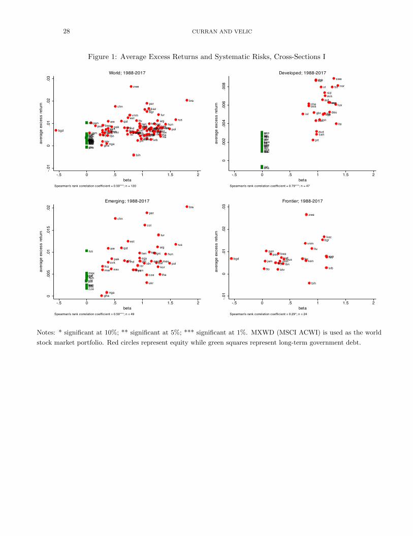
For the period 1988-2017, Figure 1 plots the cross-section of average excess returns on national

stock market indexes and 10-year government bonds against the corresponding betas obtained

from equation (11). The betas in this figure are estimated using the MSCI All Country World

Index as the global portfolio. Figure 2 repeats the exercise for the extended time interval 1968-

12 CURRAN AND VELIC

2017 by employing the MSCI Developed Markets Index as a proxy for the global portfolio.

Over the common time period, the MSCI world and developed market indexes are highly

correlated.

Figures 1 and 2 both indicate a strong positive association between the excess returns

and systematic risks of assets in world, developed, emerging and frontier market samples.

This salient feature of the graphs stands in stark contrast to the typical evidence proffered

by the literature, namely, that CAPM betas bear at best a weak postive relation with excess

returns. The graphs highlight that there is significant dispersion in country betas, with

values ranging from approximately -0.40 to 2. Moreover, beta estimates across the two

figures prove to be quite similar. As expected, long-term government bonds typically carry

the lowest betas, where the former are given by green squares while equities are denoted by

red circles. The removal of these assets however does not adversely affect the rank correlation

coefficients of world, developed, and emerging country cohorts, which lie around 0.60, 0.80,

and 0.60 respectively.6 Overall, the preliminary graphical evidence of pronounced positive

correlations suggests that market betas should have significant explanatory power in cross-

section regressions.

Table 2 displays the results of the cross-section CAPM regressions (equation (12)) for the

four aforementioned country cohorts and four different regional portfolios approximating the

global portfolio. For each global portfolio proxy, the average excess return observed in the

data is reported under the regression results, along with the average risk-free rate for the

period.

Panel A of the table uses the MSCI All Country World Index (mxwd) as the global

portfolio, and thus is based on the period 1988-2017. The panel shows that market betas

have notable explanatory power in most country samples, with the R-squared value reaching

as high as 0.63 for developed markets. Regression standard errors are relatively low too.

The estimate of the slope coefficient on beta in the case of world and developed samples

falls exactly in line with the average monthly excess global portfolio return of 0.004 (or 0.4

percent) over the period, as predicted by the CAPM.7 Such congruency with the slope of the

theoretical security market line is practically non-existent in the literature.

At 0.005, the slope estimate for emerging markets marginally overshoots the average

global portfolio risk premium, in contrast to the regular findings of significant undershooting

6Parametric Pearson correlations (unreported) are also similar.7The annualized rate is approximately 5 percent.

THE CAPM, NATIONAL STOCK MARKET BETAS, AND MACROECONOMIC COVARIATES 13

in the literature. We note, however, that an estimate of 0.004 is obtained for this group

when government bonds are omitted from the regression. Meanwhile, in the relatively small

cohort of frontier markets, the slope estimate of 0.003 marginally undershoots the target,

although it narrowly falls short of statistical significance. Despite the latter, at conventional

significance levels, additional statistical tests (unreported) in each sample still stress that one

cannot reject the null hypothesis of a slope coefficient equal to 0.004.

Intercept estimates are generally larger than the average T-Bill rate in the data (0.001)

and these differences tend to be statistically significant, as indicated by excess return regres-

sions. Nevertheless, we highlight that the intercept estimate for developed markets (0.002)

is relatively close to our average risk-free rate. Furthermore, the intercept estimate in this

sample turns out to be consistent with the average risk-free rate when bonds are excluded

from the analysis, while the slope coefficient estimate is unaffected. That is, a regression of

excess returns on betas yields a statistically insignificant constant term. Thus, a perfect fit

is retrieved in the case of equities alone in the developed markets sample. Figure 3 shows

the corresponding security market line.

Panel B of Table 2 employs the MSCI Developed Markets Index (mxwo) as the global

portfolio and covers the extended period 1968-2017. The results yielded in this panel are

virtually identical to those found in panel A, reflecting the high degree of correlation between

the aggregate world and developed market portfolios. Panel B deviates from Panel A only

with respect to the average excess global portfolio return in the data, which now stands at

0.003, making the theoretical security market line slightly flatter than before.

In panel C of the table, the MSCI Emerging Markets Index (mxef) proxies for the global

portfolio and results pertain to the interval 1988-2017 as in panel A. The coefficient estimates

on beta for world, developed and emerging market samples stand typically around 0.007, or

an annualized rate of approximately 8.7 percent. These point estimates are almost equal

to the historical average excess return of 0.008 on the global portfolio proxy. On the other

hand, the frontier market sample estimate of 0.004 is marginally statistically insignificant,

although one cannot reject the null hypothesis of a 0.008 value. In relation to the intercept

term, estimates across the four columns remain relatively similar to those in previous panels.

Overall, three of the four samples observe a higher R-squared under the emerging markets

global portfolio proxy. Most notably, market betas now explain 42 percent of the variation

in emerging market average excess returns (column (3)).

Finally, panel D in Table 2 adopts the MSCI Frontier Markets Index (mxfm) as the global

14 CURRAN AND VELIC

portfolio and spans the period 2002-2017. As in panel C, the slope coefficient estimates lie

around 0.007 for world, developed and emerging market groups. In addition now, the frontier

markets sample generates a statistically significant slope coefficient of 0.007. As can be seen

from the panel, these estimates on beta across the four samples tend to be in symmetry with

the mean monthly excess return on the global portfolio proxy, namely 0.7 percent. Intercept

terms still generally suggest overshooting of the average risk-free rate, which is approximately

zero during the period. However, this parameter now reaches its peak at 0.003 across columns,

with emerging and frontier market samples observing declines in the estimate. In particular,

the frontier market intercept estimate is borderline statistically significant at the 10 percent

level, arguably equating the empirical security market line of the sample with the theoretical

one. Relative to previous panels, the R-squared value in the frontier markets sample is higher.

5.1.2 Short Time Horizons

Given that the systematic risks of national stock markets can fluctuate over time, we also exe-

cute our time series and cross-section CAPM regressions for shorter time horizons. Long-term

averages can conceal many pertinent features of the financial landscape. This is especially

true when the time horizon is so long that it includes substantial changes in the underlying

finanical infrastructure, such as institutional and regulatory framework developments.

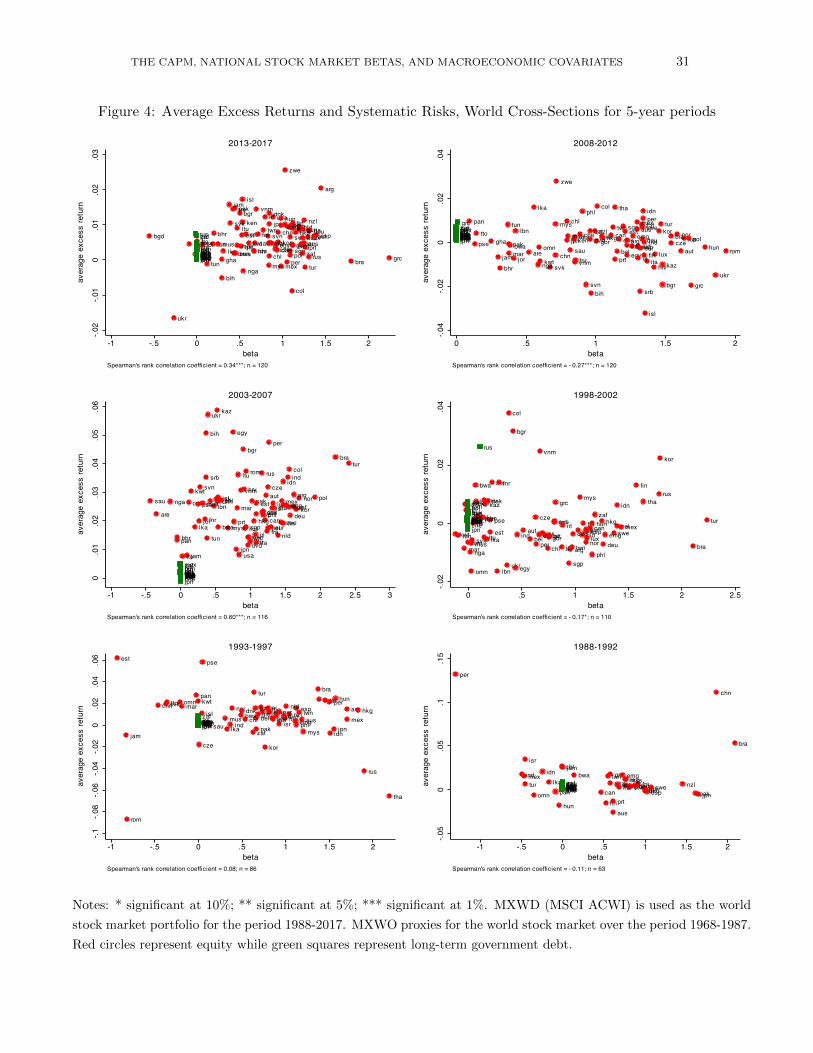
Taking a closer look at the data, Figure 4 plots cross-country average excess returns

against corresponding market betas for non-overlapping five-year periods. The graphs con-

vey the message that the risk-reward relation is not broadly consistent over the entire sample

period. For instance, in the five-year period 2003-2007 immediately prior to the global finan-

cial crisis and great recession, we observe a strong positive relation (rank correlation of 0.60)

between average excess returns on passive “buy and hold” national stock market indexes and

systematic risk. However, this relation turns significantly negative during the recessionary,

crisis period of 2008-2012 (rank correlation of -0.27), before reverting to significantly positive

in the recovery phase of 2013-2017 (rank correlation of 0.34). Other unconventional cases of

distinct negative correlations in the graphs include the period 1998-2002 when the dot com

bubble burst and 1973-1977 when the first major oil crisis of the decade hit.

Using Figure 5 we can discern that these episodes of pronounced negative correlations

coincide heavily with episodes of large return volatility in the world stock market index. For

example, the 2008-2012 interval is characterized by an annualized return volatility level of

THE CAPM, NATIONAL STOCK MARKET BETAS, AND MACROECONOMIC COVARIATES 15

approximately 21.5 percent, compared to the average level of roughly 14 percent over the full

interval 1968-2017. According to the adaptive markets hypothesis, the standard risk-reward

nexus can break down during phases of heightened equity volatility. Specifically, large abrupt

increases in stock market volatility cause a non-negligible fraction of investors to swiftly lower

their holdings through a fight-or-flight response, or, “freaking out”. Panic selling during crises

places downward pressure on equity prices and upward pressure on the prices of safer assets,

as investors reconfigure their portfolios to hold more of the latter. Such dynamics engender

a temporary violation of the positive risk-reward relation. Once overreactions subside, the

wisdom of the crowds prevails and the standard investment paradigm spawned by the efficient

markets hypothesis is restored. Thus, financial markets can be bipolar, featuring excessive

downward price spirals at times, but exhibiting normal behavior on most occasions (Lo,

2017).

Another potential explanation for the ostensibly backward relation between risk and re-

ward is the so-called “leverage effect”. Deteriorating stock markets inflict negative returns

on investors. This produces higher volatility as firms featuring debt in their capital structure

are now more highly leveraged. In turn, this can also increase national covariances with the

global market. Overall, periodic slumps may not have a significant impact over long time

horizons. Although we observe a general upward trend in equities over the very long run (e.g.

50 years), most investors do not adopt such holding positions. Examining shorter five-year

horizons can therefore be more informative.

Tables 3-5 shows the results of cross-section regressions of average returns on market betas

for different five-year periods. The MSCI world index (mxwd) is used as the global portfolio

over the interval 1988-2017, while the MSCI developed markets index (mxwo) is used as the

global portfolio over the interval 1968-1987. Panel C of Table 3 indicates that slope coefficient

estimates on beta over the 2003-2007 period were largely consistent with the corresponding

excess global portfolio return of 0.013. Indeed, the null hypothesis that 0.013 is the true

value cannot be rejected at conventional significance levels across samples. However, with

the exception of the developed markets sample, intercept estimates significantly overshoot

the average real risk-free rate of roughly zero. All country cohorts observe relatively high

R-squareds, with the developed group attaining the highest value of 0.82.

During the period 2008-2012, panel B suggests that riskier assets received a lower return.

Deviating significantly from the excess world portfolio return of 0.001, point slope estimates

are -0.004 for world and developed groups, -0.002 for emerging markets, although statisti-

16 CURRAN AND VELIC

cally insignificant, and -0.009 for frontier markets. Intercept estimates overshoot once again.

Overall, R-squared values indicate much lower explanatory power compared to the previous

period.

However, in the recovery phase of 2013-2017 following the great recession, the positive

return-beta link is restored as shown in panel A. Standing at 0.004 and 0.005 respectively,

coefficient estimates on market beta for world and developed groups fall short of the excess

global portfolio return of 0.008. Meanwhile, the frontier markets sample attains a point

estimate of 0.007 which cannot be statistically differentiated from the excess world return.

Conversely, we find a statistically insignificant estimate on beta of 0.001 for emerging markets.

According to relatively recent Geneva reports on the world economy (e.g. Buttiglione et al.

(2014)), global debt accumulation post financial crisis (2010 in particular) has continued

under the stimulus of emerging markets, with notable increases in corporate debt. This may

consequently have dampened the standard return-beta nexus for emerging markets in 2013-

2017. Intercept estimates lie around zero and are closer to the observed real risk-free rate of

-0.001. Moreover, R-squared values are higher for world and developed samples.

Panel D reveals that a negative relation between return and systematic risk generally

prevailed over the period 1998-2002, except in the case of frontier markets. In particular,

column (2) indicates that the slope and intercept point estimates for developed markets are

perfectly aligned with the average excess global portfolio return of -0.004 and average risk-free

rate of 0.002. For the entire world sample, the slope estimate is -0.002, while the intercept

estimate is 0.002 again.

Panels E, G and H of Table 4 show that the relation between beta and return is typically

positive across country samples for the periods 1993-1997, 1983-1987 and 1978-1982. In panel

E, while the point estimate on beta is 0.005 for the world sample, the corresponding estimate

for developed markets falls in line with the mean excess return on the global portfolio of 0.008.

Meanwhile, intercept estimates tend to overshoot, although not by as much in the case of

world and developed samples, and R-squareds are relatively high. In panel G, slope estimates

tend to be consistent with the excess global portfolio return of 0.010, while intercept estimates

are quite close to the risk-free rate of 0.004. In fact, at standard significance levels across

samples, normally one cannot reject the null hypotheses that slope and intercept parameters

are 0.010 and 0.004 respectively. Panel H predominantly displays statistically insignificant

coefficient estimates. At the 5 percent level across all columns, one is unable to reject the null

hypothesis of a slope coefficient equal to the average world portfolio excess return of -0.002

THE CAPM, NATIONAL STOCK MARKET BETAS, AND MACROECONOMIC COVARIATES 17

over the period 1978-1982. Furthermore, at all conventional significance levels, intercept

estimates are statistically indistinguishable from the average risk-free rate of 0.001 during

the interval.

Finally, Table 5 gives results for the periods 1973-1977 and 1968-1972. For the first of

these intervals, Panel I reveals that there is a negative link between systematic risk and

return across country samples, with slope estimates lying around the average excess global

portfolio return of -0.007. Indeed, in all cases, one cannot reject the null hypothesis that the

slope parameter is -0.007. Intercept estimates, nevertheless, overshoot the average risk-free

rate. For the second time interval, panel J highlights a positive risk-reward relation, with

slope estimates equalling approximately 0.002. These estimates fall below the excess world

portfolio return of 0.004. In contrast, the intercept estimates of around 0.002 lie above the

average risk-free rate of 0.001.

5.2 Systematic Risk in National Stock Markets

Table 6 shows the discrepancies in equity systematic risks across developed, emerging and

frontier markets over full time intervals. Regardless of the global portfolio used, panels A-D

indicate that frontier markets exhibit the lowest betas. Employing the world and developed

market indexes respectively as proxies for the global portfolio, panels A and B report median

(mean) betas of around 1.09 (1.08) for developed markets, 0.94 (0.92) for emerging markets,

and 0.38 (0.54) for frontier markets. As column (5) of the table shows, these differences

are statistically significant. With the emerging markets global potfolio proxy, panel C also

displays statistically significant differences. However, median and mean betas across samples

are now lower, with frontier markets characterized by a median beta of 0.25 compared to the

high of 0.75 for emerging markets. Using the frontier markets index as the global portfolio,

panel D indicates that group differences are not statistically significant. Based on estimates

alone, nevertheless, frontier markets have a lower median beta (roughly 0.60) than developed

and emerging markets (roughly 0.70 for both).

Providing an intertemporal decomposition, Table 7 examines country group betas over

shorter time horizons of five years. World and developed market indexes are used as the

global portfolio, with panels A-F using the former and panels G-J using the latter. We find

that frontier stock markets display the lowest levels of systematic risk in each period, while

developed stock markets are typically at the other end of the spectrum. Differences across

18 CURRAN AND VELIC

country cohorts in each period tend to be statistically significant.

Frontier markets observe the lowest level of systematic risk during 1993-1997, with a

median beta of approximately -0.01. Conversely, they are exposed to the highest level of

systematic risk during 2008-2012, with a median beta of approximately 0.72. Similarly, the

median beta for developed markets is also highest, at 1.30, in 2008-2012. The lowest beta,

on the other hand, for this group is found during 1973-1977. The relatively stronger betas

of advanced economies, particularly in more recent times, can partly be attributed to the

harmonization of national risk appetites, arising from the transmission effects induced by

monetary policy in global financial centres (Jorda et al., 2018). Meanwhile, emerging market

median betas range from 0.36 over the period 1968-1972 to 1.19 over 2003-2007. Tests of

mean and median equality over time for each country group, including the full world sample,

point to statistically significant intertemporal differences in betas.

Lastly, assessing the means and medians of pooled five-year estimates over 1968-2017,

the bottom of Table 7 shows results consistent with panels A and B of Table 6. Developed

markets carry the highest equity betas, followed by emerging, and then frontier markets.

The corresponding pooled median (mean) betas are 1.01 (1.02), 0.86 (0.86) and 0.30 (0.36)

respectively. These figures are marginally smaller than those in Table 6.

5.3 Performance

Figure 6 summarizes general stock market performance for each country over the sample

period by plotting average and median five-year Sharpe ratios and Morningstar risk-adjusted

returns. The Sharpe ratio is the reward-to-variability ratio, defined as (rp − rf)/σp. The

Morningstar rating on the other hand can be interpreted as the risk-free equivalent excess

return for an investor with a level of risk aversion γ. Specifically, with annualized values, it is

defined as [T −1∑Tt=1[(1 + rp,t)(1 + rf,t)−1]−γ]−12/γ − 1. In line with the literature, we set γ = 2.

The graphs indicate that the two general performance indicators are highly correlated,

with parametric and non-parametric correlations in excess of 0.50. Notably, the graphs sug-

gest that frontier stock markets are typically among the better performers in our sample.8 We

find pooled median 5-year Sharpe ratios of 0.29, 0.27 and 0.47 for developed, emerging and

frontier markets over the full period, where the data are annualized. Looking at pooled me-

dian 5-year Morningstar returns over the same time horizon, we obtain corresponding values

8Quite similar patterns are found over the shorter interval 1988-2017 too.

THE CAPM, NATIONAL STOCK MARKET BETAS, AND MACROECONOMIC COVARIATES 19

of 0.004, -0.053 and 0.036 respectively. These group differences are statistically significant.

However, Jensen’s alpha, which is defined as the average return on the national stock

market index over and above that predicted by the CAPM, does not suggest that frontier

markets are systematically better performers.9 Figure 7 shows that 5-year alphas across

countries and over time tend to be clustered around zero. Figure 8 in turn plots 5-year

alphas against 5-year betas across countries over the entire sample period. In contrast to

previous studies, the graph suggests that countries with higher levels of non-diversifiable

stock market risk are not systematically associated with negative alphas. In particular, we

find that the median beta across countries with positive alphas is 0.84, while it is 0.94 across

countries with negative alphas, with this discrepancy being statisitically insignificant at the

10 percent level. As the graph illustrates, there does not appear to be an unequivocally

strong inverse relation between alpha and beta.

5.4 Betas and Covariates

5.4.1 Cross-Section Correlations

Figure 9 provides cross-section plots of systematic risks in national stock markets against a

number of potential macroeconomic covariates over the full sample period of the world port-

folio index, where time-averages of the latter variables are employed.10 The initial graphical

evidence suggests strong links between country betas and corresponding macro variables.

Almost all of the supporting non-parametric gross correlation coefficients are statistically

significant at the 1 percent level.

Plots 9(a) and 9(b) show that financial and trade openness, measured by volumes of

respective stocks and flows, are positively associated with systematic risk in national equity

markets. This suggests that enhanced cross-border financial and trade linkages induce higher

comovements across countries. Economies in which it is easier to conduct business, as a result

of greater political stability or less rigid regulation for example, are expected to have more

pronounced global ties through higher levels of international portfolio investment, foreign

direct investment etc. Importantly, better business environments are more conducive to

successes among domestic firms, that, building on their foundations, can go on to compete

robustly on the world stage with their exports. As Figure 9(c) illustrates, there is a positive

9That is, Jensen’s alpha can be obtained as the intercept from time series regression (11).10The graphs do not change significantly by using median values of macro variables or the sample period

of the developed markets portfolio index.

20 CURRAN AND VELIC

relation between market betas and ease-of-doing business rankings.

Figures 9(d)-9(f) show that economic size and development factors, such as market cap-

italization and real GDP, are positively correlated with systematic risks in national equity.

Bigger economic players can impart far-reaching effects more regularly. For instance, larger

developed markets, especially global financial centres, are likely to covary more with world

markets through national monetary policy spillovers or familiarity bias in the international

portfolios of foreign investors. Conversely, local events in developing markets are less likely

to have the ubiquitous effects that induce such comovements.

The next three figures, 9(g)-9(i), depict a positive link between exchange rate volatility

(nominal or real) and beta, while a negative one between geographical distance from the

U.S. and beta. The former correlation is consistent with Bordo and Helbling (2003) who

find that fixing the exchange rate does not enhance output synchronization across countries.

Moreover, recent research finds that, post 1945, the transmission effects of financial centre

monetary policy are sizable under floats, leading to an increased synchronization of national

risk appetites that bind equity markets together (Jorda et al., 2018). The latter correlation

on the other hand may indicate that countries further away from the main actor on the world

stage are less exposed to contagion effects from the region. This may be related to weaker

financial and trade linkages with the U.S. as a result of larger information asymmetries or

transportation costs. The final plot, Figure 9(j), suggests that international reserve holdings

correlate positively with systematic risk in equity markets.

5.4.2 Five-Year Panel Regressions

Examining the macroeconomic covariates of national equity betas in a more refined longitu-

dinal setup, Table 8 provides the results of fixed effects and pooled OLS panel regressions

using five-year data. Betas in columns (1)-(3) are based on the all-country world portfolio

(acwi mxwd), with regressions corresponding to the interval 1988-2017. Betas in columns

(4)-(6) meanwhile are based on the developed markets world portfolio proxy, with regressions

corresponding to the 1968-2017 interval. Panel A of the table employs nominal exchange rate

volatility in the specifications, while panel B uses real exchange rate volatility instead. Finan-

cial openness, trade openness, market capitalization, and international reserves are employed

as fractions of national GDP.

Consistent with the preliminary cross-section analysis of gross correlations, the core fixed

THE CAPM, NATIONAL STOCK MARKET BETAS, AND MACROECONOMIC COVARIATES 21

effects panel regressions of Table 8 (columns (1) and (4)) show that financial and trade open-

ness have relatively strong positive links with national stock market betas. The parameter

estimates are all statistically significant at one or more of the conventional levels. In panel

A of the table, the estimated coefficients on financial openness stand around 0.21 and are

statistically significant at the 1 percent level. This implies that a 10 percent increase in

financial openness (i.e. percentage change in variable) is associated with a 0.021 increase

in beta. In panel B, the comparable average estimate is 0.39. Trade openness coefficient

estimates are quite sizable in fixed effects regressions, ranging from 0.56 in panel B to 0.88

in panel A. The average estimate across the four specifications suggests that a 10 percent

increase in trade openness is related to a 0.075 increase in beta, which is over twice as much

as the typical effect of a similar increase in international financial integration. Although they

are smaller, trade openness coefficients remain positive and mostly statistically significant in

pooled regressions.

Reflecting financial or economic size and development, market capitalization and relative-

to-world GDP are statistically significant covariates across all specifications in both panels

of the table. Unequivocally, all estimates point to a positive association between each of

these variables and beta. Pooled regressions, however, yield slope estimates that are less

economically significant. In particular, market capitalization coefficients across fixed effects

regressions lie around 0.16, while in pooled regressions the typical value is around 0.09. There

is a more pronounced positive relation between relative GDP and beta. Slope estimates in

this instance range from about 0.14 in pooled regressions to values of approximately 0.56 and

0.85 in fixed effects specifications.

In contrast to indications along the cross section, panel estimates suggest an inverse link

between international reserves and systematic risk in national stock markets. In panel A,

within-regression estimates for reserves of around -1.25 are much larger in absolute terms

than corresponding pooled estimates, although the latter are statistically insignificant. In

panel B, on the other hand, all slope coefficients on reserves are relatively similar in size.

They average around -0.49, but only pooled estimates are statistically significant. Overall,

our results suggest that international reserves assist in insulating national markets against

foreign shocks, thereby decoupling domestic and foreign output and equity movements.

In almost all specifications, higher exchange rate volatility is associated with a higher

equity beta. In panel B of the table, coefficients on real effective exchange rate volatility across

columns are all positive and statistically significant at the 5 percent level. The estimates are

22 CURRAN AND VELIC

similar in magnitude with a typical value of 0.13, implying that a 10 percent increase in

real exchange rate volatility contributes to a 0.013 increase in beta. For bilateral nominal

exchange rate volatility in panel A, pooled estimates are clustered around 0.05 and are

statistically significant at the 1 percent level. Conversely, corresponding estimates in fixed

effects regressions are indifferent from zero.

The primary reason for the discrepancy between pooled and within estimates of volatility

coefficients in panel A is that the nominal exchange rate exhibits much greater variation

across countries than over time for individual countries. For example, certain peggers in the

Middle East observe virtually zero nominal exchange rate volatility over the sample period.

Put differently, given that pooled regressions focus on between-country variation, while fixed

effects regressions focus on within-country variation, the former are better suited to capturing

the role of nominal exchange rate volatility. In summary, our estimates are consistent with the

notion that lower nominal exchange rate volatility raises consensus among domestic investors

about the likely direction of home fundamentals, thereby attenuating the need to look abroad

for guidance, and thus cross-border comovements.

6 Conclusions

Employing national stock market prices across the globe, this paper finds that the basic

CAPM performs much better than documented in the literature. At shorter time horizons

we also obtain evidence indicating that the positive risk-reward relation can break down

during times of high volatility, as suggested by the adaptive markets hypothesis. Relative

to advanced and emerging markets, our results point to lower systematic risk in frontier

equity markets. Moreover, general return indicators reveal that frontier stock markets have

on average fared better than more developed ones, while the relation between alphas and

betas across countries is quite flat. Examining government bond markets across nations, we

find that they are weakly related to the world portfolio, bearing very low absolute betas in

comparison to typical equities.

We next investigate the macroeconomic covariates of national stock market betas. Our

results show that countries characterized by higher levels of financial and trade openness,

exchange rate volatility, and larger economic size feature greater systematic risk in their

equity markets. On the other hand, by protecting the economy from external pressures,

international reserves are found to attenuate the systematic link between national and world

THE CAPM, NATIONAL STOCK MARKET BETAS, AND MACROECONOMIC COVARIATES 23

stock markets. Importantly, our results suggest that with increasing trade globalization, the

transmitted effects of country-specific developments are likely to be more profoundly felt in

foreign markets. In addition, such integration into the world economy implies a reduction in

the benefits of portfolio diversification across countries.

24 CURRAN AND VELIC

References

Ahn, S., Perez, M. F. and Gadarowski, C. (2013). Two-Pass Estimation of Risk Premiums

with Multicollinear and Near-Invariant Betas. Journal of Empirical Finance, 20 (C), 1–17.

Bai, H., Hou, K., Kung, H., Li, E. X. N. and Zhang, L. (2018). The CAPM Strikes Back? An

Equilibrium Model with Disasters. Journal of Financial Economics, forthcoming.

Berk, J. B. and van Binsbergen, J. H. (2016). Assessing Asset Pricing Models Using Revealed

Preference. Journal of Financial Economics, 119 (1), 1–23.

Black, F., Jensen, M. C. and Scholes, M. (1972). The Capital Asset Pricing Model: Some

Empirical Tests. In M. C. Jensen (ed.), Studies in the Theory of Capital Markets, New York:

Praeger, pp. 79–121.

Blume, M. and Friend, I. (1970). Measurement of Portfolio Performance under Uncertainty.

American Economic Review, 60 (4), 607–636.

— and — (1973). A New Look at the Capital Asset Pricing Model. Journal of Finance, 28 (1),

19–33.

Bordo, M. D. and Helbling, T. (2003). Have National Business Cycles Become More Synchro-

nized? NBER Working Paper No. 10130.

Bruno, V. and Shin, H. S. (2015). Cross-Border Banking and Global Liquidity. Review of Eco-

nomic Studies, 82 (2), 535–564.

Burnside, C., Eichenbaum, M. and Rebelo, S. (2004). Government Guarantees and Self-

Fulfilling Speculative Attacks. Journal of Economic Theory, 119 (1), 31–63.

Buttiglione, L., Lane, P. R., Reichlin, L. and Reinhart, V. (2014). Deleveraging? What

Deleveraging? Geneva Reports on the World Economy 16.

Caballero, R. and Krishnamurthy, A. (2004). Smoothing Sudden Stops. Journal of Economic

Theory, 119 (1), 104–127.

Calderon, C., Chong, A. and Stein, E. (2007). Trade Intensity and Business Cycle Synchro-

nization: Are Developing Countries Any Different? Journal of International Economics, 71 (1),

2–21.

Calomiris, C. W. and Mamaysky, H. (2018). How News and Its Context Drive Risk and Returns

Around the World. NBER Working Paper No. 24430.

THE CAPM, NATIONAL STOCK MARKET BETAS, AND MACROECONOMIC COVARIATES 25

Campbell, J. Y. (2018). Financial Decisions and Markets: A Course in Asset Pricing. Princeton,

NJ: Princeton University Press.

— and Vuolteenaho, T. (2004). Bad Beta, Good Beta. American Economic Review, 94 (5),

1249–1275.

Chinn, M. D. and Forbes, K. J. (2004). A Decomposition of Global Linkages in Financial Markets

Over Time. Review of Economics and Statistics, 86 (3), 705–722.

Chutasripanich, N. and Yetman, J. (2015). Foreign Exchange Intervention: Strategies and

Effectiveness. BIS Working Paper No. 499.

Cochrane, J. H. (2005). Asset Pricing. Princeton, NJ: Princeton University Press, revised edn.

Coeurdacier, N. and Guibaud, S. (2011). International Portfolio Diversification Is Better Than

You Think. Journal of International Money and Finance, 30 (2), 289–308.

Cook, D. and Yetman, J. (2012). Expanding Central Bank Balance Sheets in Emerging Asia:

A Compendium of Risks and Some Evidence. In Are Central Bank Balance Sheets in Asia Too

Large?, 66, BIS Papers, pp. 30–75.

Fama, E. F. and French, K. R. (1992). The Cross-Section of Expected Stock Returns. Journal

of Finance, 47 (2), 427–465.

— and — (1993). Common Risk Factors in the Returns on Stocks and Bonds. Journal of Financial

Economics, 33 (1), 3–56.

— and — (1996). Multifactor Explanations of Asset Pricing Anomolies. Journal of Finance, 51 (1),

55–84.

— and — (2004). The Capital Asset Pricing Model: Theory and Evidence. Journal of Economic

Perspectives, 18 (3), 25–46.

— and — (2006). The Value Premium and the CAPM. Journal of Finance, 61 (5), 2163–2185.

— and — (2015). A Five-Factor Asset Pricing Model. Journal of Financial Economics, 116 (1),

1–22.

— and — (2016). Dissecting Anomalies with a Five-Factor Model. Review of Financial Studies,

29 (1), 69–103.

— and MacBeth, J. D. (1973). Risk, Return, and Equilibrium: Empirical Tests. Journal of

Political Economy, 81 (3), 607–636.

26 CURRAN AND VELIC

Frankel, J. A. and Rose, A. K. (1998). The Endogeneity of the Optimum Currency Area

Criteria. Economic Journal, 108 (449), 1009–1025.

Gerlach-Kristen, P., McCauley, R. and Ueda, K. (2016). Currency Intervention and the

Global Portfolio Balance Effect: Japanese Lessons. Journal of the Japanese and International

Economies, 39 (C), 1–16.

Imbs, J. M. (2004). Trade, Finance, Specialization, and Synchronization. Review of Economics and

Statistics, 86 (3), 723–734.

— (2006). The Real Effects of Financial Integration. Journal of International Economics, 68 (2),

296–324.

Jagannathan, R. and McGrattan, E. R. (1995). The CAPM Debate. Federal Reserve Bank of

Minneapolis Quarterly Review, 19 (4), 2–17.

Jorda, O., Schularick, M., Taylor, A. M. and Ward, F. (2018). Global Financial Cycles

and Risk Premiums. CEPR Discussion Paper No. 12969.

Kalemli-Ozcan, S., Sorensen, B. E. and Yosha, O. (2001). Economic Integration, Industrial

Specialization, and the Asymmetry of Macroeconomic Fluctuations. Journal of International

Economics, 55 (1), 107–137.

King, M. and Wadhwani, S. (1990). Transmission of Volatility between Stock Markets. Review

of Financial Studies, 3 (1), 5–33.

Kose, M. A., Prasad, E. S. and Terrones, M. E. (2003). How Does Globalization Affect the

Synchronization of Business Cycles? American Economic Review, 93 (2), 57–62.

Lakonishok, J. and Shapiro, A. C. (1986). Systematic Risk, Total Risk and Size as Determinants

of Stock Market Returns. Journal of Banking and Finance, 10 (1), 115–132.

Lane, P. R. and Milesi-Ferretti, G. M. (2007). The External Wealth of Nations Mark II:

Revised and Extended Estimates of Foreign Assets and Liabilities, 1970-2004. Journal of Inter-

national Economics, 73 (2), 223–250.

Lo, A. W. (2017). Adaptive Markets: Financial Evolution at the Speed of Thought. Princeton, NJ:

Princeton University Press.

Obstfeld, M. (2015). Trilemmas and Trade-Offs: Living with Financial Globalization. BIS Work-

ing Paper No. 480.

—, Shambaugh, J. C. and Taylor, A. M. (2004). Monetary Sovereignty, Exchange Rates, and

Capital Controls: The Trilemma in the Interwar Period. IMF Staff Papers, 51 (1), 75–108.

THE CAPM, NATIONAL STOCK MARKET BETAS, AND MACROECONOMIC COVARIATES 27

—, — and — (2005). The Trilemma in History: Tradeoffs Among Exchange Rates, Monetary

Policies, and Capital Mobility. Review of Economics and Statistics, 87 (3), 423–438.

Reinganum, M. R. (1981). A New Empirical Perspective on the CAPM. Journal of Financial and

Quantitative Analysis, 16 (4), 439–462.

Rey, H. (2013). Dilemma not Trilemma: The Global Financial Cycle and Monetary Policy In-

dependence. Proceedings, Economic Policy Symposium, Jackson Hole, Federal Reserve Bank of

Kansas City. August 23-24. pp. 285–333.

Roll, R. and Ross, S. A. (1994). On the Cross-Sectional Relation between Expected Returns and

Betas. Journal of Finance, 49 (1), 101–121.

Stambaugh, R. F. (1982). On the Exclusion of Assets from Tests of the Two-Parameter Model:

A Sensitivity Analysis. Journal of Financial Economics, 10 (3), 237–268.

28 CURRAN AND VELIC

Figure 1: Average Excess Returns and Systematic Risks, Cross-Sections I

usagbrche

swe

espsgp

nornzlnld

luxita

isl deufra

findnk

bel

aus

are

ukr

tur

tha

zafsvnsau

rusqat

polmexmysken

isrind

gha

egy

cze

colchn

chl

arg

bhr

bgd

bih

bgr

hrv

jor

kaz

kwt

lbn

ltu

maromn

pakpsepan

rom

srb

lkatun

vnm

zwe

kor

prtjpn

irlgrc

can

aut

twnsvk phl

per

nga

idnhunhkg

est

bra

bwa

jam mus

ttousa

zaf

svksvnswe

rus

prtpolnzlnornld

mex

luxkor

jpn

itaislisrirlhungrcgbrfrafinespdnkdeuczechl

che

canbelausaut

dvd

emgfnr eur

-.01

0.0

1.0

2.0

3

aver

age

exce

ss re

turn

-.5 0 .5 1 1.5 2beta

Spearman's rank correlation coefficient = 0.59***; n = 120

World; 1988-2017

usa

gbr

che

swe

esp

sgp

nornzl

nld

lux

ita

isl deufra

fin

dnk

bel

aus

prt

jpn

irl

can

aut

usa

swe

prtnzlnor

nldlux

jpn

ita

isl

irl

gbrfrafin

esp

dnk

deu

che

canbel

aus

aut

dvd

eur

0.0

02.0

04.0

06.0

08

aver

age

exce

ss re

turn

-.5 0 .5 1 1.5 2beta

Spearman's rank correlation coefficient = 0.79***; n = 47

Developed; 1988-2017

are

ukr

tur

tha

zaf

svnsau

rusqat

polmex

mysisr

ind

gha

egy

cze

col

chn

chl

arg

mar

pak

lka kor

grctwn

svk phl

per

nga

idn

hunhkg

est

bra

zaf

svksvn

rus

pol

mex

korisr

hungrc

cze

chl

emg

0.0

05.0

1.0

15.0

2

aver

age

exce

ss re

turn

-.5 0 .5 1 1.5 2beta

Spearman's rank correlation coefficient = 0.59***; n = 49

Emerging; 1988-2017

ken

bhr

bgd

bih

bgr

hrv

jor

kaz

kwt

lbn

ltu

omn

psepan

rom

srbtun

vnm

zwe

bwa

jam mus

tto

fnr

-.01

0.0

1.0

2.0

3

aver

age

exce

ss re

turn

-.5 0 .5 1 1.5 2beta

Spearman's rank correlation coefficient = 0.29*; n = 24

Frontier; 1988-2017

Notes: * significant at 10%; ** significant at 5%; *** significant at 1%. MXWD (MSCI ACWI) is used as the world

stock market portfolio. Red circles represent equity while green squares represent long-term government debt.

THE CAPM, NATIONAL STOCK MARKET BETAS, AND MACROECONOMIC COVARIATES 29

Figure 2: Average Excess Returns and Systematic Risks, Cross-Sections II

usagbrche

swe

espsgp

nornzlnld

luxita

isl deufra

findnk

bel

aus

are

ukr

tur

tha

zafsvnsau

rusqat

polmexmysken

isrind

gha

egy

cze

colchn

chl

arg

bhr

bgd

bih

bgr

hrv

jor

kaz

kwt

lbn

ltu

maromn

pakpsepan

rom

srb

lkatun

vnm

zwe

kor

prtjpn

irlgrc

can

aut

twnsvk phl

per

nga

idnhunhkg

est

bra

bwa

jam mus

ttousa

zaf

svksvnswe

rus

prtpolnzlnornld

mex

luxkor

jpn

itaislisrirlhungrcgbrfrafinespdnkdeuczechl

che

canbelausaut

wld

emgfnr eur

-.01

0.0

1.0

2.0

3

aver

age

exce

ss re

turn

-.5 0 .5 1 1.5 2beta

Spearman's rank correlation coefficient = 0.57***; n = 120

World; 1968-2017

usa

gbr

che

swe

esp

sgp

nornzl

nld

lux

ita

isl deufra

fin

dnk

bel

aus

prt

jpn

irl

can

aut

usa

swe

prtnzlnor

nldlux

jpn

ita

isl

irl

gbrfrafin

esp

dnk

deu

che

canbel

aus

aut

eur

0.0

02.0

04.0

06.0

08

aver

age

exce

ss re

turn

-.5 0 .5 1 1.5 2beta

Spearman's rank correlation coefficient = 0.78***; n = 46

Developed; 1968-2017

are

ukr

tur

tha

zaf

svnsau

rusqat

polmex

mysisr

ind

gha

egy

cze

col

chn

chl

arg

mar

pak

lka kor

grctwn

svk phl

per

nga

idn

hunhkg

est

bra

zaf

svksvn

rus

pol

mex

korisr

hungrc

cze

chl

emg

0.0

05.0

1.0

15.0

2

aver

age

exce

ss re

turn

-.5 0 .5 1 1.5 2beta

Spearman's rank correlation coefficient = 0.58***; n = 49

Emerging; 1968-2017

ken

bhr

bgd

bih

bgr

hrv

jor

kaz

kwt

lbn

ltu

omn

psepan

rom

srbtun

vnm

zwe

bwa

jam mus

tto

fnr

-.01

0.0

1.0

2.0

3

aver

age

exce

ss re

turn

-.5 0 .5 1 1.5 2beta

Spearman's rank correlation coefficient = 0.26*; n = 24

Frontier; 1968-2017

Notes: * significant at 10%; ** significant at 5%; *** significant at 1%. MXWO is used as the world stock market

portfolio. Red circles represent equity while green squares represent long-term government debt.

30 CURRAN AND VELIC

Figure 3: Empirical Security Market Line, 1988-2017

usa

gbr

che

swe

esp

sgp

nor

nzl

nld

lux

ita

isl

deufra

findnk

bel

aus

prt

jpn

irl

can

aut

dvd

eur

.002

.004

.006

.008

.01

aver

age

mon

thly

retu

rn (%

)

.6 .8 1 1.2 1.4beta

Notes: Sample consists of developed national stock markets. Global portfolio employed is the MSCI All Country World

Index (MXWD). Security market line (SML) plotted is both the empirical and theoretical one. SML has a slope of

0.004, consistent with the average monthly excess return on the world portfolio over the period. When national stock

market beta is equal to 0, SML shows an average monthly return equal to 0.001, consistent with the average risk-free

rate over the period.

THE CAPM, NATIONAL STOCK MARKET BETAS, AND MACROECONOMIC COVARIATES 31

Figure 4: Average Excess Returns and Systematic Risks, World Cross-Sections for 5-year periods

usa

gbr

cheswe esp

sgpnor

nzlnld

luxita

isl

deufrafin

dnk

bel

aus

are

ukr

tur

thazaf

svnsau

rusqat

pol

mexmys

ken

isr

ind

gha

egycze

col

chn

chl

arg

bhrbgd

bih

bgr

hrvjor

kazkwtlbn

ltu

maromn

pak

psepan

romsrb

lka

tun

vnm

zwe

korprt

jpnirl

grccan

auttwn

svk

phl

pernga

idn

hun

hkgest

brabwa

jam

mustto

usa

zaf

svksvnswe

rus

prtpolnzlnornld

mex

luxkorjpnitaislisrirlhun

grc

gbrfrafinespdnkdeuczechl

checanbelausaut

dvd

emg

fnreur

-.02

-.01

0.0

1.0

2.0

3

aver

age

exce

ss re

turn

-1 -.5 0 .5 1 1.5 2beta

Spearman's rank correlation coefficient = 0.34***; n = 120

2013-2017

usagbr

cheswe

esp

sgpnornzl

nldlux

ita

isl

deufra

fin

dnk

bel

aus

are

ukr

tur

tha

zaf

svn

sau

rusqat

pol

mexmys

ken isrindgha

egy

cze

col

chn

chl

arg

bhr

bihbgr

hrvjor

kazkwt

lbn

ltumar

omnpakpse

pan

rom

srb

lka

tun

vnm

zwe

kor

prt

jpn

irl

grc

can

aut

twn

svk

phlper

nga

idn

hunhkg

estbra

bwa

jam

musttousazafsvksvnswerusprtpolnzlnornldmexluxkorjpnitaislisrirlhungrc

gbrfrafinespdnkdeuczechlchecanbelausaut dvd emg

fnr

eur

-.04

-.02

0.0

2.0

4

aver

age

exce

ss re

turn

0 .5 1 1.5 2beta

Spearman's rank correlation coefficient = - 0.27***; n = 120

2008-2012

usa

gbrche

sweesp

sgp

nor

nzlnld

lux

ita

isl

deu

frafin

dnk

bel

ausare

ukr

tur

tha zaf

svn

sau

rus

qat polmex

mys

isr

ind

egy

cze

col

chn

chl

arg

bhr

bih

bgr

hrv

jor

kaz

kwt

lbn

ltu

maromn pakpse

pan

romsrb

lka

tun

vnm

kor

prt

jpn

irl

grc

can

aut

twn

svkphl

per

nga

idn

hun

hkg

est

bra

bwa

jam

mus

tto

usazafsvksvnswerusprtpolnzlnornld

mex

luxkorjpnitaislisrirlhungrcgbrfrafinespdnkdeuczechlchecanbelausaut

dvd

emg

fnreur

0.0

1.0

2.0

3.0

4.0

5.0

6

aver

age

exce

ss re

turn

-1 -.5 0 .5 1 1.5 2 2.5 3beta

Spearman's rank correlation coefficient = 0.60***; n = 116

2003-2007

usagbrche sweesp

sgp

nor

nzl

nldlux

isl

deu

fra

fin

dnkbel

aus

are

ukr

tur

tha

zafsau

rusqat

polmex

mys

isrind

egy

cze

col

chn

chl arg

bgr

hrv

jor

kaz

kwt

lbn

ltu

mar

omn

pak

psepan

rom lkatun

vnmkor

prt

jpn

irl

grc

canaut

twnsvk

phlper

nga

idn

hunhkg

est

bra

bwa

jam

mus

ttousa

zafsvksvn

swe

rus

prt

polnzlnornld

mex

luxkor

jpnitaislisrirlhungrcgbrfrafinespdnkdeuczechecanbelausaut

dvd emg

fnr

eur

-.02

0.0

2.0

4

aver

age

exce

ss re

turn

0 .5 1 1.5 2 2.5beta

Spearman's rank correlation coefficient = - 0.17*; n = 110

1998-2002

usagbrche

sweespnor

nzlnld

isl deufra

findnk

bel aus

tur

tha

zafsau

rus

pol mex

mysisrind

cze

chn

chlarg

kwt

lbn

maromn

pak

pse

pan

rom

lka

kor

prt

jpn

irlgrc canaut

twnsvk

phl

per

idn

hun

hkg

est

bra

bwa

jam

mus

tto

usazafsweprtnzlnornldluxjpnitaislisrirlgrcgbrfrafinespdnkdeuchecanbelausaut

dvdemg

eur

-.1-.0

8-.0

6-.0

4-.0

20

.02

.04

.06

aver

age

exce

ss re

turn

-1 -.5 0 .5 1 1.5 2beta

Spearman's rank correlation coefficient = 0.08; n = 86

1993-1997

usagbrche sweesp

nzlnlddeufra

finaus

turmex mys

isr

ind

chn

chl

omn pakpanlka

kor

prtjpnirl

grc

canaut

twnphl

per

idn

hun

hkg

bra

bwajam

musttousa

zafswenzlnornldjpnitaislirlgbrfrafinespdnkdeuchecanbelausaut dvd

emg

-.05

0.0

5.1

.15

aver

age

exce

ss re

turn

-1 -.5 0 .5 1 1.5 2beta

Spearman's rank correlation coefficient = - 0.11; n = 63

1988-1992

Notes: * significant at 10%; ** significant at 5%; *** significant at 1%. MXWD (MSCI ACWI) is used as the world

stock market portfolio for the period 1988-2017. MXWO proxies for the world stock market over the period 1968-1987.

Red circles represent equity while green squares represent long-term government debt.

32 CURRAN AND VELIC

Figure 4 (continued): Average Excess Returns and Systematic Risks, World Cross-Sections for 5-yearperiods

usagbr

che

swe

espnlddeu

fra

fin

mysind

lka korjpn irl

grc

canaut

twn

phl

idn

hkg

jamtto

usazafswenzlnornldirlgbrfraespdnkdeuchecanbelaus

-.06

-.04

-.02

0.0

2.0

4.0

6.0

8.1

aver

age

exce

ss re

turn

-.5 0 .5 1 1.5beta

Spearman's rank correlation coefficient = 0.28*; n = 40

1983-1987

usa

deu

mys

ind

kor

jpn can

twn

hkg

usazafnzl

nld

irl

gbrfraesp

deu

che

canbelaus

-.01

-.005

0.0

05.0

1

aver

age

exce

ss re

turn

0 .5 1 1.5beta

Spearman's rank correlation coefficient = 0.18; n = 22

1978-1982

usa

deu

mys

jpn

can

twn

hkgusazaf

nzlnld

irlgbrfradeu

che

canbelaus

-.01

0.0

1.0

2

aver

age

exce

ss re

turn

0 .5 1 1.5 2beta

Spearman's rank correlation coefficient = - 0.32*; n = 19

1973-1977

usa

deu

jpn

can

twn

hkg

usazafnzlnld

irlgbrfradeuchecanbelaus0

.01

.02

.03

.04

aver

age

exce

ss re

turn

0 .2 .4 .6 .8 1beta

Spearman's rank correlation coefficient = 0.50**; n = 18

1968-1972

Notes: * significant at 10%; ** significant at 5%; *** significant at 1%. MXWD (MSCI ACWI) is used as the world

stock market portfolio for the period 1988-2017. MXWO proxies for the world stock market over the period 1968-1987.

Red circles represent equity while green squares represent long-term government debt.

THE CAPM, NATIONAL STOCK MARKET BETAS, AND MACROECONOMIC COVARIATES 33

Figure 5: World Stock Market Index, Rolling 5-year Return Volatility

.03

.04

.05

.06

retu

rn v

olat

ility

1970:12 1980:12 1990:12 2000:12 2010:12 2020:125-year period

Notes: The horizontal axis marks the end of each 5-year period. The red dashed line marks the average return volatility

over the entire sample period.

34 CURRAN AND VELIC

Figure 6: Average (left) and Median (right) 5-Year Performance Indicators, 1968-2017

aus

autbel

can

che

deu

dnk

dvd

esp

eurfin

fra

gbr

irlisl

ita jpn

lux

nldnor

nzl

prt sgp

sweusawld

are

arg

bra chlchn

col

cze egy

emg

est

gha

grc hkg

hunidn

ind

isr

kor

lka

mar

mex

mys

nga

pak

per

phl

pol

qat

russau

svk

svn

tha

turtwn

ukr

zaf

bgd

bgr

bhr

bih

bwa

fnr

hrv

jam

jor

kaz

ken

kwt

lbn

ltu

mus

omn

pan

pse

rom

srb

tto tun

vnm

zwe

0.3

.6.9

1.2

shar

pe ra

tio

-.2 -.1 0 .1morningstar risk-adjusted return

ausaut

bel

canche

deu

dnk

dvd

esp

eur

fin

fragbr

irl

isl

ita

jpnlux

nld

nor

nzl

prt

sgpswe

usawld

are

arg

brachlchn

col

czeegy

emg

est

gha

grchkg

hun

idnind

isrkorlka

mar

mex

mys

nga

pak

per

phl

pol

qat

russau

svk

svn

tha

tur

twn

ukr

zaf

bgd

bgr

bhr

bih

bwa

fnr

hrv

jamjor

kazken

kwtlbn

ltu mus

omn

pan

pse

rom

srb

tto

tun

vnm zwe

-.6-.3

0.3

.6.9

1.2

shar

pe ra

tio

-.3 -.2 -.1 0 .1 .2morningstar risk-adjusted return

Notes: Blue circles, red squares, and green triangles correspond to developed, emerging, and frontier stock markets

respectively. Annualized figures are shown.

THE CAPM, NATIONAL STOCK MARKET BETAS, AND MACROECONOMIC COVARIATES 35

Figure 7: 5-Year Alphas

ausaus aus aus

ausautaut

aut aut

aut

aut autbel belbel belcan can

cancan can can can can can

canche

cheche che che chedeu

deu

deudeu deu deu

deu deu deu deudnk

dnkdnk

dnkdnk

dvd dvd dvd dvd dvd dvd dvd dvd dvd dvdespesp esp

espesp esp

eur eur eureur eur

fin

finfin

finfin

finfra

fra fra fra fra fragbr gbr gbrgbr gbr gbr gbr

irlirl

irlirl irl

irlirlisl

isl

isl

isl

islita

itaita

jpn

jpn jpnjpn

jpnjpn

jpn jpn jpn jpnluxlux

lux luxnld nld nld

nld nld nld nldnor

nornor

nornor

nzl nzl nzl nzl nzlprt

prtprt

prt

prt prtsgp

sgp sgpsgp

swe

sweswe

swe swe swesweusa usa usa

usausa usa usa usa usa usawld wld wld wld wld wld

areare

are

arearg

arg

argarg

arg

bra

bra

bra

bra

bra

bra

chl

chlchl

chl chl

chl

chn

chn

chn

chn

chnchn

col col

colcze

czecze

cze czeegy

egy

egy egy

emg

emgemg

emgemg

emg

est

est

estest estgha gha

grcgrc grc grc

grc grc

hkg

hkghkg hkg

hkghkg

hkg hkghkg hkg

hun

hunhun hun

hunhun

idn

idn

idn

idn idn idn

idnind ind

ind

ind ind

ind

ind indisr isrisr

isr isrkor

korkor

kor

kor

kor korkor

lkalka

lka lka

lka lka

lka

mar

mar

mar

mar marmex

mexmex mex mex

mex

mys

mys

mys

mys

mys mys mys

mysnga

nga

nga ngapak pak

pakpak

pakpak

per

per

per

per

per

per

phlphl phl

phlphl

phlpol pol pol polpol

qat

qat

qat qat

rusrus

rusrus

sau sau

sau

sau sau

svk

svk

svk

svk

svk

svn

svn

svn

tha

tha thatha

thatur

tur

tur tur tur

tur

twntwn

twn

twntwn

twntwn

twn twn twn

ukr

ukr

ukr ukrzaf

zaf zaf zaf

zaf

bgd

bgr bgr

bgr

bgrbhr

bhr

bhr

bih

bih

bih

bwabwa

bwa bwabwa bwa

fnr

fnrfnr

hrv

hrvhrv

jam

jamjam jam

jam

jamjor

jor

jorjorkaz

kaz

kazkazkenken

kwt

kwt

kwt

kwtkwtlbn

lbn

lbn

lbn lbnltu

ltu

ltultumus mus

mus

mus

mus mus

omn

omn

omn

omn omn

pan

panpan pan

panpse

pse

psepse

rom

rom

romrom

srb

srb

srb

tto

tto

tto

tto tto tto ttotun

tun tuntun

vnmvnm

vnm

vnm

zwezwe

-.1-.0

50

.05

.1.1

5je

nsen

's a

lpha

1970 1980 1990 2000 2010 20205-year period

Notes: Blue circles, red squares, and green triangles correspond to developed, emerging, and frontier stock markets

respectively. The horizontal axis marks the final year of each non-overlapping 5-year period. Jensen’s alpha is the

average return on the national stock market portfolio over and above that predicted by the CAPM.

Figure 8: Alphas vs Betas

-.1-.0

50

.05

.1.1

5je

nsen

's a

lpha

-1 0 1 2 3beta

Notes: Blue circles, red squares, and green triangles correspond to developed, emerging, and frontier stock markets

respectively. 5-year alphas and betas are employed. Jensen’s alpha is the average return on the national stock market

portfolio over and above that predicted by the CAPM. Parametric and non-parametric correlations between alpha

and beta are close to zero.

36 CURRAN AND VELIC

Figure 9: Betas vs. Covariates over the Cross Section

usagbr

che

sweesp

sgp

nor

nzl

nld

luxita

isl

deufra

fin

dnk bel

aus

are

ukr

turthazaf

svn

sau

rus

qat

pol

mex

myskenisr

ind

gha

egyczecol

chn

chl

arg

bhr

bgd

bih

bgrhrv

jor

kaz

kwtlbn

ltu

maromnpak

psepan

romsrb

lka tun

vnmzwe

kor

prtjpnirl

grc

canaut

twn

svk

phlper

nga

idn

hun

hkg

est

bra

bwa

jam

mus

tto

eur

-.50

.51

1.5

2be

ta

8 10 12 14 16 18ln(financial openness)

Spearman's rank correlation coefficient = 0.58***; n = 83

usagbr

che

sweespsgp

nor

nzl

nld

lux ita

isl

deufra

fin

dnk bel

aus

are

ukr

turthazaf

svn

sau

rus

qat

pol

mex

myskenisr

ind

gha

egyczecol

chn

chl

arg

bhr

bgd

bih

bgrhrv kaz

kwtlbn

ltu

maromnpak

psepan

romsrb

lkatun

vnmzwe

kor

prtjpnirl

grc

canaut

svk

phlper

nga

idn

hun

hkg

est

bra

bwa

jam

mus

tto

eur

-.50

.51

1.5

2be

ta

8 10 12 14 16ln(trade openness)

Spearman's rank correlation coefficient = 0.55***; n = 82

(a) (b)

usagbr

che

sweesp

sgp

nor

nzl

nld

luxita

isl

deufra

fin

dnk bel

aus

are

ukr

turthazaf

svn

sau

rus

qat

pol

mex

mys kenisr

ind

gha

egycze col

chn

chl

arg

bhr

bgd

bih

bgrhrv

jor

kaz

kwt lbn

ltu

maromnpak

psepan

romsrb

lkatun

vnm zwe

kor

prtjpnirl

grc

canaut

svk

phlper

nga

idn

hun

hkg

est

bra

bwa

jam

mus

tto

-.50

.51

1.5

2be

ta

0 50 100 150 200doing business indicator

Spearman's rank correlation coefficient = - 0.45***; n = 82

usagbr

che

sweesp

sgp

nor

nzl

nld

lux itadeu

frafin

dnk bel

aus

are

ukr

turthazaf

svn

sau

rus

qat

pol

mex

myskenisr

ind

gha

egycze col

chn

chl

arg

bhr

bgd

bgrhrv

jor

kaz

kwtlbnmaromn

pak

psepan

romsrb

lkatun

vnmzwe

kor

prtjpnirl

grc

canaut

svk

phlper

nga

idn

hun

hkg

bra

bwa

jam

mus

tto

eur

-.50

.51

1.5

2be

ta

6 8 10 12 14 16ln(market capitalization)

Spearman's rank correlation coefficient = 0.50***; n = 78

(c) (d)

usagbr

che

sweesp

sgp

nor

nzl

nld

lux ita

isl

deufra

fin

dnkbel

aus

are

ukr

turthazaf

svn

sau

rus

qat

pol

mex

myskenisr

ind

gha

egyczecol

chn

chl

arg

bhr

bgd

bih

bgrhrv

jor

kaz

kwtlbn

ltu

maromnpak

psepan

romsrb

lkatun

vnmzwe

kor

prtjpnirl

grc

canaut

svk

phlper

nga

idn

hun

hkg

est

bra

bwa

jam

mus

tto

eur

-.50

.51

1.5

2be

ta

8 10 12 14 16 18ln(real GDP)

Spearman's rank correlation coefficient = 0.58***; n = 82

usagbr

che

sweesp

sgp

nor

nzl

nld

luxita

isl

deufrafin

dnkbel

aus

are

ukr

turthazaf

svn

sau

rus

qat

pol

mex

myskenisr

ind

gha

egyczecol

chn

chl

arg

bhr

bgd

bih

bgrhrv

jor

kaz

kwtlbn

ltu

mar omnpak

psepan

romsrb

lka tun

vnmzwe

kor

prtjpnirl

grc

canaut

svk

phlper

nga

idn

hun

hkg

est

bra

bwa

jam

mus

tto

eur

-.50

.51

1.5

2be

ta

6 8 10 12ln(real GDP per capita)

Spearman's rank correlation coefficient = 0.35***; n = 82

(e) (f)

THE CAPM, NATIONAL STOCK MARKET BETAS, AND MACROECONOMIC COVARIATES 37

Figure 9 (continued): Betas vs. Covariates over the Cross Section

gbrche

sweesp

sgp

nor

nzl

nld

luxita

isl

deufra

fin

dnkbel

aus

are

ukr

turthazaf

svn

sau

ruspol

mex

myskenisr

ind

gha

egyczecol

chn

chl

arg

bhr

bgd

bih

bgrhrv

jor

kaz

kwt lbn

ltu

maromnpak

romsrb

lkatun

vnm zwe

kor

prtjpnirl

grc

canaut

svk

phlper

nga

idn

hun

hkg

est

bra

bwa

jam

mus

tto

eur

-.50

.51

1.5

2be

ta

-20 -15 -10 -5 0 5 10ln(nominal exchange rate volatility)

Spearman's rank correlation coefficient = 0.41***; n = 81

usagbr

che

sweesp

sgp

nor

nzl

nld

lux ita

isl

deufra

fin

dnkbel

aus ukr

zaf

sau

ruspol

mex

mysisr

gha

cze col

chn

chl

bhr

bgrhrv

mar

pak

rom

tun

kor

prtjpnirl

grc

canaut

svk

phl

nga

hun

bra

tto

-.50

.51

1.5

2be

ta

-4 -3.5 -3 -2.5 -2 -1.5ln(real exchange rate volatility)

Spearman's rank correlation coefficient = 0.09; n = 51

(g) (h)

usagbr

che

sweesp

sgp

nor

nzl

nld

lux ita

isl

deufra

fin

dnkbel

aus

are

ukr

tur thazaf

svn

sau

rus

qat

pol

mex

myskenisr

ind

gha

egyczecol

chn

chl

arg

bhr

bgd

bih

bgrhrv

jor

kaz

kwtlbn

ltu

mar omnpak

pan

romsrb

lkatun

vnmzwe

kor

prtjpnirl

grc

canaut

twn

svk

phlper

nga

idn

hun

hkg

est

bra

bwa

jam

mus

tto

-.50

.51

1.5

2be

ta

0 5000 10000 15000 20000distance (km)

Spearman's rank correlation coefficient = - 0.20*; n = 82

usagbr

che

sweesp

sgp

nor

nzl

nld

lux ita

isl

deufra

fin

dnkbel

aus

are

ukr

tur thazaf

svn

sau

rus

qat

pol

mex

myskenisr

ind

gha

egyczecol

chn

chl

arg

bhr

bgd

bih

bgrhrv

jor

kaz

kwtlbn

ltu

maromnpak

pan

romsrb

lka tun

vnmzwe

kor

prtjpnirl

grc

canaut

svk

phlper

nga

idn

hun

est

bra

bwa

jam

mus

tto

-.50

.51

1.5

2be

ta

6 8 10 12 14ln(reserves)

Spearman's rank correlation coefficient = 0.47***; n = 79

(i) (j)

Notes: * significant at 10%; ** significant at 5%; *** significant at 1%. Period employed is 1988-2017.

38 CURRAN AND VELIC

Tab

le1:

Cou

ntry

and

Corresp

ondin

gSto

ckM

arketIn

dex

Lists

Develop

edC

ountries

Em

erging

Cou

ntries

Fron

tierC

ountries

Cou

ntry

Code

BB

GIn

dex

Cou

ntry

Code

BB

GIn

dex

Cou

ntry

Code

BB

GIn

dex

1A

ustralia

AU

SA

S52

1A

rgentin

aA

RG

BU

RC

AP

1B

ahrain

BH

RB

HSE

ASI

2A

ustria

AU

TA

TX

2B

razilB

RA

IBO

V2

Ban

gladesh

BG

DD

SE

X3

Belgiu

mB

EL

BE

LP

RC

3C

hile

CH

LIG

PA

3B

osnia

&H

erzegovin

aB

IHSA

SX

-104

Can

ada

CA

NSP

TSX

4C

hin

a(P

RC

)C

HN

SH

CO

MP

4B

otswan

aB

WA

BG

SM

DC

5D

enm

arkD

NK

KA

X5

Colom

bia

CO

LC

OL

CA

P5

Bulgaria

BG

RSO

FIX

6F

inlan

dF

INH

EX

6C

zechR

epublic

CZ

EP

X6

Croatia

HR

VC

RO

7F

rance

FR

AC

AC

7E

gypt

EG

YE

GX

307

Jam

aicaJA

MJM

SM

X8

Germ

any

DE

UD

AX

8E

stonia

EST

TA

LSE

8Jord

anJO

RJO

SM

GN

FF

9Icelan

dIS

LIC

EX

I9

Ghan

aG

HA

GG

SE

CI

9K

azakhstan

KA

ZK

ZK

AK

10Irelan

dIR

LIS

EQ

10G

reeceG

RC

ASE

10K

enya

KE

NN

SE

ASI

11Italy

ITA

ITL

MS

11H

ong

Kon

gH

KG

HSI

11K

uw

aitK

WT

KW

SE

IDX

12Jap

anJP

NN

KY

12H

ungary

HU

NB

UX

12L

eban

onL

BN

BL

OM

13L

uxem

bou

rgL

UX

LU

XX

X13

India

IND

SE

NSE

X13

Lith

uan

iaLT

UV

ILSE

14N

etherlan

ds

NL

DA

EX

14In

don

esiaID

NJC

I14

Mau

ritius

MU

SSE

MD

EX

15N

ewZ

ealand

NZ

LN

ZSE

15Israel

ISR

TA

-3515

Om

anO

MN

MSM

3016

Norw

ayN

OR

OSE

BX

16K

orea,R

ep.

KO

RK

OSP

I16

Palestin

eP

SE

PA

SIS

I17

Portu

galP

RT

BV

LX

17M

alaysia

MY

SF

BM

KL

CI

17P

anam

aP

AN

BV

PSB

VP

S18

Sin

gapore

SG

PST

I18

Mex

icoM

EX

INM

EX

18R

oman

iaR

OM

BE

T19

Spain

ESP

IBE

X19

Moro

ccoM

AR

MC

SIN

DE

X19

Serb

iaSR

BB

EL

EX

LIN

20Sw

eden

SW

EO

MX

20N

igeriaN

GA

NG

SE

IND

X20

Trin

idad

&T

obago

TT

OT

TC

OM

P21

Sw

itzerland

CH

ESP

I21

Pak

istanP

AK

KSE

10021

Tunisia

TU

NT

USIS

E22

United

Kin

gdom

GB

RU

KX

22P

eruP

ER

SP

BL

25PT

22V

ietnam

VN

MV

NIN

DE

X23

United

States

USA

SP

X23

Philip

pin

esP

HL

PC

OM

P23

Zim

bab

we

ZW

EZ

HIN

DU

SD

24P

oland

PO

LW

IG20

AW

orld

Mark

ets

WL

DM

XW

D25

Qatar

QA

TD

SM

EFro

ntie

rM

ark

ets

FN

RM

XF

MB

Develo

ped

Mark

ets

DV

DM

XW

O26

Russia

RU

SIN

DE

XC

FC

Eu

roM

ark

ets

EU

RM

XE

M27

Sau

di

Arab

iaSA

USA

SE

IDX

28Slovak

iaSV

KSK

SM

29Sloven

iaSV

NSB

ITO

P30

Sou

thA

fricaZ

AF

JA

LSH

31Sri

Lan

kaL

KA

CSE

AL

L32

Taiw

anT

WN

TW

SE

33T

hailan

dT

HA

SE

T50

34T

urkey

TU

RX

U100

35U

krain

eU

KR

PF

TS

36U

AE

AR

EA

DSM

I

DE

merg

ing

Mark

ets

EM

GM

XE

F

Notes:

Country

classifi

cations

arebased

up

onth

oseavailab

lefrom

MSC

Iand

Calom

irisand

Mam

aysk

y(201

8).M

ostcou

ntries

have

asin

glecon

stant

classification

overth

etim

ein

terval.F

or

eachcou

ntry

we

use

the

classification

that

fits

the

country

forth

em

ajo

rityof

the

sample

perio

d.

THE CAPM, NATIONAL STOCK MARKET BETAS, AND MACROECONOMIC COVARIATES 39

Table 2: Cross-Section CAPM Regressions: Long Time Horizons

(1) (2) (3) (4)Sample World Developed Emerging Frontier

A. world portfolio: acwi mxwd

Beta 0.004∗∗∗ 0.004∗∗∗ 0.005∗∗∗ 0.003(0.001) (0.000) (0.001) (0.002)

Constant 0.003∗∗∗ 0.002∗∗∗ 0.004∗∗∗ 0.005∗∗∗

(0.000) (0.000) (0.001) (0.001)Sigma 0.004 0.002 0.004 0.006R-squared 0.26 0.63 0.34 0.05Observations 120 47 49 24

Average excess world portfolio return 0.004Average risk-free rate 0.001

B. world portfolio: mxwo

Beta 0.004∗∗∗ 0.004∗∗∗ 0.005∗∗∗ 0.003(0.001) (0.000) (0.001) (0.002)

Constant 0.003∗∗∗ 0.002∗∗∗ 0.004∗∗∗ 0.005∗∗∗

(0.000) (0.000) (0.001) (0.001)Sigma 0.004 0.002 0.004 0.006R-squared 0.25 0.65 0.33 0.05Observations 120 46 49 24

Average excess world portfolio return 0.003Average risk-free rate 0.001

C. world portfolio: mxef

Beta 0.007∗∗∗ 0.006∗∗∗ 0.007∗∗∗ 0.004(0.001) (0.001) (0.001) (0.003)

Constant 0.003∗∗∗ 0.002∗∗∗ 0.003∗∗∗ 0.006∗∗∗

(0.000) (0.000) (0.001) (0.001)Sigma 0.004 0.002 0.004 0.006R-squared 0.32 0.59 0.42 0.06Observations 120 47 48 24

Average excess world portfolio return 0.008Average risk-free rate 0.001

D. world portfolio: mxfm

Beta 0.007∗∗∗ 0.006∗∗∗ 0.007∗∗∗ 0.007∗

(0.001) (0.001) (0.002) (0.004)Constant 0.003∗∗∗ 0.002∗∗∗ 0.003∗∗∗ 0.003∗

(0.000) (0.000) (0.001) (0.002)Sigma 0.004 0.002 0.004 0.006R-squared 0.32 0.62 0.29 0.14Observations 120 47 49 23

Average excess world portfolio return 0.007Average risk-free rate 0.000

Notes: * significant at 10%; ** significant at 5%; *** significant at 1%. Robuststandard errors in parentheses.

40 CURRAN AND VELIC

Table 3: Cross-Section CAPM Regressions: Short Time Horizons I

(1) (2) (3) (4)Sample World Developed Emerging Frontier

A. 2013-2017

Beta 0.004∗∗∗ 0.005∗∗∗ 0.001 0.007∗

(0.001) (0.001) (0.002) (0.004)Constant 0.001∗∗∗ 0.000∗∗ 0.002 0.003∗

(0.001) (0.000) (0.002) (0.002)Sigma 0.005 0.003 0.006 0.006R-squared 0.10 0.48 0.01 0.17Observations 120 47 49 24

Average excess world portfolio return 0.008Average risk-free rate −0.001

B. 2008-2012

Beta −0.004∗∗∗ −0.004∗∗∗ −0.002 −0.009∗∗

(0.001) (0.001) (0.002) (0.004)Constant 0.002∗∗∗ 0.002∗∗∗ 0.003∗∗ 0.002

(0.001) (0.000) (0.001) (0.003)Sigma 0.008 0.006 0.008 0.010R-squared 0.07 0.17 0.02 0.18Observations 120 47 49 24

Average excess world portfolio return 0.001Average risk-free rate −0.001

C. 2003-2007

Beta 0.013∗∗∗ 0.015∗∗∗ 0.012∗∗∗ 0.024∗∗∗

(0.001) (0.001) (0.002) (0.005)Constant 0.010∗∗∗ 0.001∗∗ 0.014∗∗∗ 0.018∗∗∗

(0.002) (0.001) (0.003) (0.003)Sigma 0.012 0.004 0.012 0.011R-squared 0.32 0.82 0.35 0.32Observations 116 47 48 21

Average excess world portfolio return 0.013Average risk-free rate 0.000

D. 1998-2002

Beta −0.002∗∗ −0.004∗∗∗ −0.000 0.038∗∗∗

(0.001) (0.001) (0.002) (0.011)Constant 0.002∗∗ 0.002∗∗∗ 0.003 −0.001

(0.001) (0.000) (0.002) (0.002)Sigma 0.009 0.010R-squared 0.00 0.36Observations 110 45 46 18

Average excess world portfolio return −0.004Average risk-free rate 0.002

Notes: * significant at 10%; ** significant at 5%; *** significant at 1%. Robuststandard errors in parentheses. Robust regressions employed where appropri-ate.

THE CAPM, NATIONAL STOCK MARKET BETAS, AND MACROECONOMIC COVARIATES 41

Table 4: Cross-Section CAPM Regressions: Short Time Horizons II

(1) (2) (3) (4)Sample World Developed Emerging Frontier

E. 1993-1997

Beta 0.005∗∗∗ 0.008∗∗∗ −0.012 0.050(0.002) (0.002) (0.007) (0.032)

Constant 0.006∗∗∗ 0.005∗∗∗ 0.015∗∗∗ 0.016(0.001) (0.001) (0.005) (0.010)

Sigma 0.005 0.020 0.030R-squared 0.42 0.17 0.34Observations 86 44 32 10

Average excess world portfolio return 0.008Average risk-free rate 0.002

F. 1988-1992

Beta −0.001 −0.003∗ −0.001 0.048∗∗∗

(0.011) (0.002) (0.017) (0.011)Constant 0.010∗∗ 0.003∗∗∗ 0.026∗∗ 0.009

(0.005) (0.001) (0.011) (0.005)Sigma 0.024 0.007 0.037 0.011R-squared 0.002 0.04 0.000 0.42Observations 63 37 20 6

Average excess world portfolio return −0.001Average risk-free rate 0.002

G. 1983-1987

Beta 0.010∗∗∗ 0.010∗∗∗ 0.014(0.002) (0.002) (0.022)

Constant 0.006∗∗∗ 0.005∗∗∗ 0.009(0.001) (0.001) (0.013)

SigmaR-squaredObservations 40 28 10

Average excess world portfolio return 0.010Average risk-free rate 0.004

H. 1978-1982

Beta 0.002 −0.000 0.010(0.002) (0.002) (0.005)

Constant 0.001 0.002∗∗ −0.004(0.001) (0.001) (0.004)

Sigma 0.005 0.004 0.007R-squared 0.06 0.001 0.42Observations 22 16 6

Average excess world portfolio return −0.002Average risk-free rate 0.001

Notes: * significant at 10%; ** significant at 5%; *** significant at 1%. Robuststandard errors in parentheses. Robust regressions employed where appropri-ate.

42 CURRAN AND VELIC

Table 5: Cross-Section CAPM Regressions: Short Time Horizons III

(1) (2) (3) (4)Sample World Developed Emerging Frontier

I. 1973-1977

Beta −0.004∗ −0.007∗∗∗ −0.007(0.002) (0.002) (0.005)

Constant 0.003∗ 0.001 0.012(0.002) (0.001) (0.008)

Sigma 0.006 0.010R-squared 0.11 0.38Observations 19 15 6

Average excess world portfolio return −0.007Average risk-free rate −0.001

J. 1968-1972

Beta 0.002∗ 0.002∗

(0.001) (0.001)Constant 0.002∗∗∗ 0.002∗∗∗

(0.000) (0.000)SigmaR-squaredObservations 18 15

Average excess world portfolio return 0.004Average risk-free rate 0.001

Notes: * significant at 10%; ** significant at 5%; *** significant at 1%. Robuststandard errors in parentheses. Robust regressions employed where appropri-ate.

THE CAPM, NATIONAL STOCK MARKET BETAS, AND MACROECONOMIC COVARIATES 43

Table 6: Systematic Risks: Long Time Horizons

Equity (1) (2) (3) (4) (5)World Developed Emerging Frontier Test of Equality

A. world portfolio: acwi mxwdmean 0.87 1.08 0.94 0.54 0.000median 0.96 1.09 0.96 0.39 0.000observations 86 25 37 24 86

B. world portfolio: dm mxwomean 0.85 1.09 0.90 0.55 0.000median 0.95 1.09 0.92 0.38 0.000observations 86 24 37 24 85

C. world portfolio: em mxefmean 0.58 0.60 0.72 0.36 0.000median 0.58 0.59 0.75 0.25 0.007observations 86 25 36 24 85

D. world portfolio: fm mxfmmean 0.67 0.68 0.72 0.58 0.127median 0.70 0.69 0.71 0.61 0.252observations 86 25 37 23 85

Notes: P-values reported for tests of equality in column (5). F*-test used for test of equal sub-group means. Mood’s median test used for test of equal sub-group medians. In correspondingorder, panels A, B, C and D pertain to the time intervals 1988-2017, 1968-2017, 1988-2017 and2002-2017 respectively.

44 CURRAN AND VELIC

Table 7: Systematic Risks: Short Time Horizons

Equity (1) (2) (3) (4) (5)World Developed Emerging Frontier Test of Equality

A. 2013-2017mean 0.82 1.11 0.88 0.42 0.000median 0.87 1.12 0.87 0.44 0.000observations 86 25 37 24 86

B. 2008-2012mean 1.05 1.22 1.10 0.77 0.001median 1.14 1.30 1.14 0.72 0.014observations 86 25 37 24 86

C. 2003-2007mean 0.92 1.14 1.06 0.41 0.000median 0.96 1.18 1.19 0.37 0.000observations 82 25 36 21 82

D. 1998-2002mean 0.70 0.93 0.84 0.14 0.000median 0.70 0.97 0.75 0.10 0.000observations 77 24 35 18 77

E. 1993-1997mean 0.70 0.89 0.85 −0.13 0.000median 0.77 0.88 0.85 −0.01 0.002observations 61 22 29 10 61

F. 1988-1992mean 0.52 0.89 0.36 −0.04 0.001median 0.62 0.88 0.55 −0.00 0.004observations 42 17 19 6 42

G. 1983-1987mean 0.67 0.90 0.46 0.14 0.002median 0.85 0.94 0.39 0.14 0.014observations 24 13 9 2 24

H. 1978-1982mean 0.78 0.99 0.61 0.201median 0.80 0.90 0.44 0.294observations 9 4 5 0 9

I. 1973-1977mean 0.83 0.85 0.80 0.946median 0.79 0.84 0.66 0.270observations 7 4 3 0 7

J. 1968-1972mean 0.73 0.92 0.36 0.132median 0.79 0.97 0.36 0.083observations 6 4 2 0 6

Test of Equality Over Timemeans 0.000 0.000 0.014 0.000medians 0.006 0.003 0.005 0.000

1968-2017, panel over 5-year intervalsmean 0.81 1.02 0.86 0.36 0.000median 0.86 1.01 0.86 0.30 0.000observations 479 163 212 104 479

Notes: P-values reported for tests of equality in column (5) and Test of Equality Over Time. F*-test used for test ofequal sub-group/period means. Mood’s median test used for test of equal sub-group/period medians.

THE CAPM, NATIONAL STOCK MARKET BETAS, AND MACROECONOMIC COVARIATES 45

Table 8: 5-Year Panel Regressions

world portfolio: acwi mxwd dm mxwo(1) (2) (3) (4) (5) (6)

Fixed Pooled Pooled Fixed Pooled PooledEffects OLS I OLS II Effects OLS I OLS II

A.

financial openness 0.216∗∗∗ −0.019 −0.006 0.210∗∗∗ −0.012 0.010(0.069) (0.042) (0.042) (0.080) (0.040) (0.040)

trade openness 0.877∗∗ 0.067 0.133 0.783∗∗ 0.084 0.160∗

(0.378) (0.098) (0.104) (0.387) (0.095) (0.100)market cap. 0.150∗∗ 0.074∗∗ 0.084∗∗ 0.177∗∗ 0.092∗∗∗ 0.112∗∗∗

(0.075) (0.038) (0.041) (0.077) (0.035) (0.037)relative gdp 0.552∗ 0.151∗∗∗ 0.148∗∗∗ 0.564∗∗ 0.147∗∗∗ 0.134∗∗∗

(0.323) (0.026) (0.025) (0.283) (0.025) (0.024)reserves −1.207∗ −0.135 −0.095 −1.286∗ −0.168 −0.113

(0.701) (0.157) (0.154) (0.688) (0.161) (0.158)exchange rate vol. I −0.019 0.050∗∗∗ 0.047∗∗∗ −0.024 0.047∗∗∗ 0.044∗∗∗

(0.054) (0.019) (0.016) (0.050) (0.018) (0.015)Time dummies yes yes no yes yes noWithin R-squared 0.38 0.41Between R-squared 0.25 0.27Overall R-squared 0.16 0.33 0.22 0.17 0.35 0.22

B.

financial openness 0.340∗ −0.031 0.008 0.429∗∗ −0.022 0.016(0.210) (0.055) (0.052) (0.214) (0.055) (0.051)

trade openness 0.791∗∗ 0.196∗ 0.232∗∗ 0.556∗ 0.208∗∗ 0.249∗∗

(0.331) (0.110) (0.110) (0.326) (0.108) (0.109)market cap. 0.145∗ 0.093∗∗ 0.072∗ 0.160∗ 0.097∗∗∗ 0.076∗

(0.089) (0.041) (0.043) (0.088) (0.038) (0.041)relative gdp 0.878∗∗∗ 0.109∗∗∗ 0.138∗∗∗ 0.813∗∗∗ 0.111∗∗∗ 0.143∗∗∗

(0.255) (0.033) (0.031) (0.275) (0.033) (0.031)reserves −0.444 −0.598∗∗∗ −0.397∗∗ −0.418 −0.644∗∗∗ −0.423∗∗

(0.686) (0.199) (0.191) (0.688) (0.193) (0.190)exchange rate vol. II 0.095∗∗ 0.145∗∗ 0.145∗∗ 0.117∗∗ 0.135∗∗ 0.133∗∗

(0.050) (0.062) (0.063) (0.053) (0.059) (0.059)Time dummies yes yes no yes yes noWithin R-squared 0.48 0.48Between R-squared 0.19 0.21Overall R-squared 0.12 0.29 0.21 0.12 0.31 0.23

Notes: * significant at 10%; ** significant at 5%; *** significant at 1%. Robust standard errors inparentheses. Dependent variable is the national stock market beta. Exchange rate vol. I (II) is nominal(real) exchange rate volatility.