
user's guide gua de usuario user's guide gua de usuario user's guide gua de usuario
Upload
julian1972mxCategory
view
214download
0
8/20/2019 MFRAC User's Guide
http://slidepdf.com/reader/full/mfrac-users-guide 1/1019
User’s Guide Ninth Edition
M eyer Frac turing
Simulators
Meyer & Associates, Inc.

8/20/2019 MFRAC User's Guide
http://slidepdf.com/reader/full/mfrac-users-guide 2/1019
ii
Meyer & Associates, Inc. Meyer User’s Guide
Information in this document is subject to change without notice. No part of this document or theassociated software may be reproduced or transmitted in any form or by any means, electronic or mechanical, for any purpose, other than as permitted in the license agreement, without the expressedwritten permission of Meyer & Associates, Inc. (Meyer).
Copyright © 1997, 1999, 2003-2011 Meyer & Associates, Inc. All rights reserved. Printed in the
United States of America.
MFrac, MF2d, MAcid, MPwri, MView, MAcq, MinFrac, MProd, MNpv, MFast, MFrac-Lite,MShale, and MWell are trademarks of Meyer & Associates, Inc.
Microsoft, MS-DOS, Windows and Word are registered trademarks of the Microsoft Corporation.
All names of companies, wells, persons or products contained in this documentation are part of ficti-tious scenarios and are used solely to document the use of a Meyer & Associates, Inc. product.
Software License Agreement
License Grant
This License Agreement permits you to use one copy of the Meyer software program(s) included inthe package. Meyer grants to the end user, a nonexclusive, nontransferable license, with no right tosublicense or prepare derivative works from the program(s) in connection with your computers.
Warranty
Meyer hereby warrants that it has the right to license the program(s). Meyer agrees to defend, indem-nify and hold harmless the end user against claims or alleged claims of infringement of any patent,copyright or other intellectual property rights.
The licensed software is provided “as-is.” All warranties and representations of any kind with regardto the licensed software are hereby disclaimed, including the implied warranties of merchantabilityand fitness for a particular purpose. Under no circumstances will Meyer & Associates, Inc. be liablefor any consequential, incidental, special or exemplary damages even if appraised of the likelihood of such damages occurring.
The licensed software includes libraries which are licensed under the Common Public License (CPL).Any provisions of this agreement which differ from the CPL are offered by Meyer alone and not byany other party.
Vendor Databases
The databases provided with the software are based on sound engineering practices, but because of variable well conditions and other information which must be relied upon, Meyer & Associates, Inc.

8/20/2019 MFRAC User's Guide
http://slidepdf.com/reader/full/mfrac-users-guide 3/1019
Meyer User’s Guide Meyer & Associates, Inc.
i
and its database suppliers make, no warranty, express or implied, as to the accuracy of their data or of any calculations or opinions expressed therein or derived therefrom. You agree that Meyer & Associ-ates, Inc. and its database suppliers shall not be liable for any loss or damage whether do to negli-gence or otherwise arising out of or concerning such data, calculations or opinions.
Third Party Acknowledgements
ICU License - ICU 1.8.1 and later
COPYRIGHT AND PERMISSION NOTICE
Copyright © 1995-2008 International Business Machines Corporation and others
All rights reserved.
Permission is hereby granted, free of charge, to any person obtaining a copy of this software and asso-ciated documentation files (the "Software"), to deal in the Software without restriction, includingwithout limitation the rights to use, copy, modify, merge, publish, distribute, and/or sell copies of theSoftware, and to permit persons to whom the Software is furnished to do so, provided that the abovecopyright notice(s) and this permission notice appear in all copies of the Software and that both theabove copyright notice(s) and this permission notice appear in supporting documentation.
THE SOFTWARE IS PROVIDED "AS IS", WITHOUT WARRANTY OF ANY KIND, EXPRESSOR IMPLIED, INCLUDING BUT NOT LIMITED TO THE WARRANTIES OF MERCHANT-ABILITY, FITNESS FOR A PARTICULAR PURPOSE AND NONINFRINGEMENT OF THIRDPARTY RIGHTS. IN NO EVENT SHALL THE COPYRIGHT HOLDER OR HOLDERSINCLUDED IN THIS NOTICE BE LIABLE FOR ANY CLAIM, OR ANY SPECIAL INDIRECTOR CONSEQUENTIAL DAMAGES, OR ANY DAMAGES WHATSOEVER RESULTING FROMLOSS OF USE, DATA OR PROFITS, WHETHER IN AN ACTION OF CONTRACT, NEGLI-GENCE OR OTHER TORTIOUS ACTION, ARISING OUT OF OR IN CONNECTION WITHTHE USE OR PERFORMANCE OF THIS SOFTWARE.
Except as contained in this notice, the name of a copyright holder shall not be used in advertising or otherwise to promote the sale, use or other dealings in this Software without prior written authoriza-tion of the copyright holder.
All trademarks and registered trademarks mentioned herein are the property of their respective own-ers.
UNICODE, INC. LICENSE AGREEMENT - DATA FILES AND SOFTWARE
Unicode Data Files include all data files under the directories http://www.unicode.org/Public/, http://www.unicode.org/reports/, and http://www.unicode.org/cldr/data/ . Unicode Software includes any

8/20/2019 MFRAC User's Guide
http://slidepdf.com/reader/full/mfrac-users-guide 4/1019
iv
Meyer & Associates, Inc. Meyer User’s Guide
source code published in the Unicode Standard or under the directories http://www.unicode.org/Pub-lic/, http://www.unicode.org/reports/, and http://www.unicode.org/cldr/data/.
NOTICE TO USER: Carefully read the following legal agreement. BY DOWNLOADING,INSTALLING, COPYING OR OTHERWISE USING UNICODE INC.'S DATA FILES ("DATAFILES"), AND/OR SOFTWARE ("SOFTWARE"), YOU UNEQUIVOCALLY ACCEPT, AND
AGREE TO BE BOUND BY, ALL OF THE TERMS AND CONDITIONS OF THIS AGREE-MENT. IF YOU DO NOT AGREE, DO NOT DOWNLOAD, INSTALL, COPY, DISTRIBUTE OR USE THE DATA FILES OR SOFTWARE.
COPYRIGHT AND PERMISSION NOTICE
Copyright © 1991-2007 Unicode, Inc. All rights reserved. Distributed under the Terms of Use inhttp://www.unicode.org/copyright.html.
Permission is hereby granted, free of charge, to any person obtaining a copy of the Unicode data filesand any associated documentation (the "Data Files") or Unicode software and any associated docu-mentation (the "Software") to deal in the Data Files or Software without restriction, including withoutlimitation the rights to use, copy, modify, merge, publish, distribute, and/or sell copies of the DataFiles or Software, and to permit persons to whom the Data Files or Software are furnished to do so,
provided that (a) the above copyright notice(s) and this permission notice appear with all copies of theData Files or Software, (b) both the above copyright notice(s) and this permission notice appear inassociated documentation, and (c) there is clear notice in each modified Data File or in the Softwareas well as in the documentation associated with the Data File(s) or Software that the data or softwarehas been modified.
THE DATA FILES AND SOFTWARE ARE PROVIDED "AS IS", WITHOUT WARRANTY OFANY KIND, EXPRESS OR IMPLIED, INCLUDING BUT NOT LIMITED TO THE WARRAN-TIES OF MERCHANTABILITY, FITNESS FOR A PARTICULAR PURPOSE AND NONIN-FRINGEMENT OF THIRD PARTY RIGHTS. IN NO EVENT SHALL THE COPYRIGHTHOLDER OR HOLDERS INCLUDED IN THIS NOTICE BE LIABLE FOR ANY CLAIM, OR ANY SPECIAL INDIRECT OR CONSEQUENTIAL DAMAGES, OR ANY DAMAGES WHAT-SOEVER RESULTING FROM LOSS OF USE, DATA OR PROFITS, WHETHER IN AN ACTIONOF CONTRACT, NEGLIGENCE OR OTHER TORTIOUS ACTION, ARISING OUT OF OR INCONNECTION WITH THE USE OR PERFORMANCE OF THE DATA FILES OR SOFTWARE.
Except as contained in this notice, the name of a copyright holder shall not be used in advertising or otherwise to promote the sale, use or other dealings in these Data Files or Software without prior writ-ten authorization of the copyright holder.
Independent JPEG Group
The Meyer software is based in part on the work of the Independent JPEG Group.

8/20/2019 MFRAC User's Guide
http://slidepdf.com/reader/full/mfrac-users-guide 5/1019
Meyer User’s Guide Meyer & Associates, Inc.
Libpng
The Meyer software includes libpng, which is:
Copyright © 1998-2008 Glenn Randers-Pehrson
Copyright © 1996-1997 Andreas Dilger
Copyright © 1995-1996 Guy Eric Schalnat, Group 42, Inc.
The Meyer software includes software developed by Greg Roelofs and contributers for the book,“PNG: The Definitive Guide,” published by O’Reilly and Associates.
Lua License
Lua is licensed under the terms of the MIT license reproduced below. This means that Lua is free soft-ware and can be used for both academic and commercial purposes at absolutely no cost.
For details and rationale, see http://www.lua.org/license.html .
Copyright © 1994-2008 Lua.org, PUC-Rio.
Permission is hereby granted, free of charge, to any person obtaining a copy of this software and asso-ciated documentation files (the "Software"), to deal in the Software without restriction, includingwithout limitation the rights to use, copy, modify, merge, publish, distribute, sublicense, and/or sellcopies of the Software, and to permit persons to whom the Software is furnished to do so, subject tothe following conditions:
• The above copyright notice and this permission notice shall be included in all copies or substan-tial portions of the Software.
THE SOFTWARE IS PROVIDED "AS IS", WITHOUT WARRANTY OF ANY KIND, EXPRESSOR IMPLIED, INCLUDING BUT NOT LIMITED TO THE WARRANTIES OF MERCHANT-ABILITY, FITNESS FOR A PARTICULAR PURPOSE AND NONINFRINGEMENT. IN NOEVENT SHALL THE AUTHORS OR COPYRIGHT HOLDERS BE LIABLE FOR ANY CLAIM,DAMAGES OR OTHER LIABILITY, WHETHER IN AN ACTION OF CONTRACT, TORT OR OTHERWISE, ARISING FROM, OUT OF OR IN CONNECTION WITH THE SOFTWARE OR THE USE OR OTHER DEALINGS IN THE SOFTWARE.
PCRE LICENSE
PCRE is a library of functions to support regular expressions whose syntax and semantics are as closeas possible to those of the Perl 5 language.

8/20/2019 MFRAC User's Guide
http://slidepdf.com/reader/full/mfrac-users-guide 6/1019
vi
Meyer & Associates, Inc. Meyer User’s Guide
Release 7 of PCRE is distributed under the terms of the "BSD" licence, as specified below. The docu-mentation for PCRE, supplied in the "doc" directory, is distributed under the same terms as the soft-ware itself.
The basic library functions are written in C and are freestanding. Also included in the distribution is aset of C++ wrapper functions.
THE BASIC LIBRARY FUNCTIONS
Written by: Philip Hazel
Email local part: ph10
Email domain: cam.ac.uk
University of Cambridge Computing Service,
Cambridge, England.
Copyright © 1997-2009 University of Cambridge
All rights reserved.
THE C++ WRAPPER FUNCTIONS
Contributed by: Google Inc.
Copyright © 2007-2008, Google Inc.
All rights reserved.
THE "BSD" LICENCE
Redistribution and use in source and binary forms, with or without modification, are permitted pro-vided that the following conditions are met:
• Redistributions of source code must retain the above copyright notice, this list of conditions andthe following disclaimer.
• Redistributions in binary form must reproduce the above copyright notice, this list of conditionsand the following disclaimer in the documentation and/or other materials provided with the dis-
tribution.• Neither the name of the University of Cambridge nor the name of Google Inc. nor the names of
their contributors may be used to endorse or promote products derived from this software withoutspecific prior written permission.

8/20/2019 MFRAC User's Guide
http://slidepdf.com/reader/full/mfrac-users-guide 7/1019
Meyer User’s Guide Meyer & Associates, Inc.
v
THIS SOFTWARE IS PROVIDED BY THE COPYRIGHT HOLDERS AND CONTRIBUTORS"AS IS" AND ANY EXPRESS OR IMPLIED WARRANTIES, INCLUDING, BUT NOT LIMITEDTO, THE IMPLIED WARRANTIES OF MERCHANTABILITY AND FITNESS FOR A PARTICU-LAR PURPOSE ARE DISCLAIMED. IN NO EVENT SHALL THE COPYRIGHT OWNER OR CONTRIBUTORS BE LIABLE FOR ANY DIRECT, INDIRECT, INCIDENTAL, SPECIAL,EXEMPLARY, OR CONSEQUENTIAL DAMAGES (INCLUDING, BUT NOT LIMITED TO,
PROCUREMENT OF SUBSTITUTE GOODS OR SERVICES; LOSS OF USE, DATA, OR PROF-ITS; OR BUSINESS INTERRUPTION) HOWEVER CAUSED AND ON ANY THEORY OF LIA-BILITY, WHETHER IN CONTRACT, STRICT LIABILITY, OR TORT (INCLUDING
NEGLIGENCE OR OTHERWISE) ARISING IN ANY WAY OUT OF THE USE OF THIS SOFT-WARE, EVEN IF ADVISED OF THE POSSIBILITY OF SUCH DAMAGE.
WTL
The Meyer software uses a modified version of the Windows Template Library (WTL). Source codefor this modified version is available on our website.
yaml-cpp License
The Meyer software uses the yaml-cpp library which is:
Copyright © 2008 Jesse Beder.
Permission is hereby granted, free of charge, to any person obtaining a copy of this software and asso-ciated documentation files (the "Software"), to deal in the Software without restriction, includingwithout limitation the rights to use, copy, modify, merge, publish, distribute, sublicense, and/or sellcopies of the Software, and to permit persons to whom the Software is furnished to do so, subject tothe following conditions:
• The above copyright notice and this permission notice shall be included in all copies or substan-tial portions of the Software.
THE SOFTWARE IS PROVIDED "AS IS", WITHOUT WARRANTY OF ANY KIND, EXPRESSOR IMPLIED, INCLUDING BUT NOT LIMITED TO THE WARRANTIES OF MERCHANT-ABILITY, FITNESS FOR A PARTICULAR PURPOSE AND NONINFRINGEMENT. IN NOEVENT SHALL THE AUTHORS OR COPYRIGHT HOLDERS BE LIABLE FOR ANY CLAIM,DAMAGES OR OTHER LIABILITY, WHETHER IN AN ACTION OF CONTRACT, TORT OR OTHERWISE, ARISING FROM, OUT OF OR IN CONNECTION WITH THE SOFTWARE OR THE USE OR OTHER DEALINGS IN THE SOFTWARE.

8/20/2019 MFRAC User's Guide
http://slidepdf.com/reader/full/mfrac-users-guide 8/1019
viii
Meyer & Associates, Inc. Meyer User’s Guide
“A fact is a simple statement that everyone believes. It is innocent,unless found guilty. A hypothesis is a novel suggestion that no onewants to believe. It is guilty, until found effective.”
- Edward Teller

8/20/2019 MFRAC User's Guide
http://slidepdf.com/reader/full/mfrac-users-guide 9/1019
ix Meyer & Associates, Inc.
Table of Contents
Introduction _________________________________________ xxxvi
Overview . . . . . . . . . . . . . . . . . . . . . . . . . . . . . . . . . . . . . . . . . .xxxvii
Program Descriptions. . . . . . . . . . . . . . . . . . . . . . . . . . . . . . . xxxviii
MFrac . . . . . . . . . . . . . . . . . . . . . . . . . . . . . . . . . . . . . . . . . . . . . . . . . xxxviiiMView . . . . . . . . . . . . . . . . . . . . . . . . . . . . . . . . . . . . . . . . . . . . . . . . . . xxxixMinFrac . . . . . . . . . . . . . . . . . . . . . . . . . . . . . . . . . . . . . . . . . . . . . . . . . xxxixMProd . . . . . . . . . . . . . . . . . . . . . . . . . . . . . . . . . . . . . . . . . . . . . . . . . . xxxix
MNpv . . . . . . . . . . . . . . . . . . . . . . . . . . . . . . . . . . . . . . . . . . . . . . . . . . . . . .xlMFast. . . . . . . . . . . . . . . . . . . . . . . . . . . . . . . . . . . . . . . . . . . . . . . . . . . . . .xlMPwri. . . . . . . . . . . . . . . . . . . . . . . . . . . . . . . . . . . . . . . . . . . . . . . . . . . . . .xlMFrac-Lite . . . . . . . . . . . . . . . . . . . . . . . . . . . . . . . . . . . . . . . . . . . . . . . . . .xlMWell. . . . . . . . . . . . . . . . . . . . . . . . . . . . . . . . . . . . . . . . . . . . . . . . . . . . . xliMShale . . . . . . . . . . . . . . . . . . . . . . . . . . . . . . . . . . . . . . . . . . . . . . . . . . . xli
About this Guide . . . . . . . . . . . . . . . . . . . . . . . . . . . . . . . . . . . . . . .xli
What’s in this Guide?. . . . . . . . . . . . . . . . . . . . . . . . . . . . . . . . . . . . . . . . . xliiTechnical Support Documentation . . . . . . . . . . . . . . . . . . . . . . . . . . xliv
How to use this Guide . . . . . . . . . . . . . . . . . . . . . . . . . . . . . . . . . . . . . . . xlviLimited Experience with Meyer Software and Fracture Design . . . . xlviGeneral Knowledge of Meyer Software and Fracturing . . . . . . . . . . xlviExperienced with Meyer Software and Fracturing . . . . . . . . . . . . . . xlvi
Symbols and Conventions. . . . . . . . . . . . . . . . . . . . . . . . . . . . . .xlvi
Chapter 1
Getting Started _________________________________________ 1.1 Introduction . . . . . . . . . . . . . . . . . . . . . . . . . . . . . . . . . . . . . . . . .1
1.2 System & Hardware Requirements . . . . . . . . . . . . . . . . . . . . . .1

8/20/2019 MFRAC User's Guide
http://slidepdf.com/reader/full/mfrac-users-guide 10/1019
x Table of Contents
Meyer & Associates, Inc. Meyer User’s Guide
1.3 Installing the Meyer Software . . . . . . . . . . . . . . . . . . . . . . . . . 2
Before Installing. . . . . . . . . . . . . . . . . . . . . . . . . . . . . . . . . . . . . . . . . . . . . . 2To Install the Meyer Applications . . . . . . . . . . . . . . . . . . . . . . . . . . . . . . . . 3Program Maintenance - Modify, Repair or Remove . . . . . . . . . . . . . . . . . . 4Database Installation. . . . . . . . . . . . . . . . . . . . . . . . . . . . . . . . . . . . . . . . . . 5
1.4 General Application Information . . . . . . . . . . . . . . . . . . . . . . . 5 Application Installation Directories . . . . . . . . . . . . . . . . . . . . . . . . . . . . . . . 6 Application Data Folder Support . . . . . . . . . . . . . . . . . . . . . . . . . . . . . . . . . 6 Application File Name Extensions. . . . . . . . . . . . . . . . . . . . . . . . . . . . . . . . 6
General . . . . . . . . . . . . . . . . . . . . . . . . . . . . . . . . . . . . . . . . . . . . . . . . . 6 Application File Extension Summary. . . . . . . . . . . . . . . . . . . . . . . . . . . . . . 7Long File Name Support . . . . . . . . . . . . . . . . . . . . . . . . . . . . . . . . . . . . . . . 8Working Files. . . . . . . . . . . . . . . . . . . . . . . . . . . . . . . . . . . . . . . . . . . . . . . . 8Read Only Files. . . . . . . . . . . . . . . . . . . . . . . . . . . . . . . . . . . . . . . . . . . . . . 9Last Opened Files . . . . . . . . . . . . . . . . . . . . . . . . . . . . . . . . . . . . . . . . . . . . 9
1.5 Starting the Software . . . . . . . . . . . . . . . . . . . . . . . . . . . . . . . . 9
Connecting the Hardware Security Key . . . . . . . . . . . . . . . . . . . . . . . . . . . 9
1.6 Quick Start . . . . . . . . . . . . . . . . . . . . . . . . . . . . . . . . . . . . . . . . 10
Program Check List. . . . . . . . . . . . . . . . . . . . . . . . . . . . . . . . . . . . . . . . . . 10
1.7 Customer Support. . . . . . . . . . . . . . . . . . . . . . . . . . . . . . . . . . 10
Updating Your Hardware Key - MKey Utility . . . . . . . . . . . . . . . . . . . . . . . 11
1.8 Windows Fundamentals . . . . . . . . . . . . . . . . . . . . . . . . . . . . . 11
1.9 Meyer Program Basics . . . . . . . . . . . . . . . . . . . . . . . . . . . . . . 11
Button Conventions. . . . . . . . . . . . . . . . . . . . . . . . . . . . . . . . . . . . . . . . . . 11File Management. . . . . . . . . . . . . . . . . . . . . . . . . . . . . . . . . . . . . . . . . . . . 12
Opening a File. . . . . . . . . . . . . . . . . . . . . . . . . . . . . . . . . . . . . . . . . . . 12Creating a New File . . . . . . . . . . . . . . . . . . . . . . . . . . . . . . . . . . . . . . 14Saving a File . . . . . . . . . . . . . . . . . . . . . . . . . . . . . . . . . . . . . . . . . . . . 14
Selecting a Printer . . . . . . . . . . . . . . . . . . . . . . . . . . . . . . . . . . . . . . . . . . . 15Defining the System Units . . . . . . . . . . . . . . . . . . . . . . . . . . . . . . . . . . . . . 17
Setting the Input and Output Units . . . . . . . . . . . . . . . . . . . . . . . . . . . 19
Getting Help . . . . . . . . . . . . . . . . . . . . . . . . . . . . . . . . . . . . . . . . . . . . . . . 19 Accessing Help . . . . . . . . . . . . . . . . . . . . . . . . . . . . . . . . . . . . . . . . . . 19Error Checking . . . . . . . . . . . . . . . . . . . . . . . . . . . . . . . . . . . . . . . . . . . . . 20
Data Entry Errors . . . . . . . . . . . . . . . . . . . . . . . . . . . . . . . . . . . . . . . . 20Run-Time Error Checking . . . . . . . . . . . . . . . . . . . . . . . . . . . . . . . . . . 21
8/20/2019 MFRAC User's Guide
http://slidepdf.com/reader/full/mfrac-users-guide 11/1019
Meyer User’s Guide Meyer & Associates, Inc.
Table of Contents x
File Version Checking . . . . . . . . . . . . . . . . . . . . . . . . . . . . . . . . . . . . . 23Working with Spreadsheets and Dialogs . . . . . . . . . . . . . . . . . . . . . . . . . . 23
Spreadsheet Keyboard Commands . . . . . . . . . . . . . . . . . . . . . . . . . . 23Spreadsheet Mouse Actions . . . . . . . . . . . . . . . . . . . . . . . . . . . . . . . . 25Freezing Spreadsheet Panes . . . . . . . . . . . . . . . . . . . . . . . . . . . . . . . 26Spreadsheet Options Dialog . . . . . . . . . . . . . . . . . . . . . . . . . . . . . . . . 27
Spreadsheet Speed Buttons . . . . . . . . . . . . . . . . . . . . . . . . . . . . . . . . 28Dialog and Spreadsheet Column Sizing . . . . . . . . . . . . . . . . . . . . . . . 30Spreadsheets With Movable Columns . . . . . . . . . . . . . . . . . . . . . . . . 31
Working with Plots . . . . . . . . . . . . . . . . . . . . . . . . . . . . . . . . . . . . . . . . . . . 33 Arranging Plot Windows . . . . . . . . . . . . . . . . . . . . . . . . . . . . . . . . . . . 33Moving Plots . . . . . . . . . . . . . . . . . . . . . . . . . . . . . . . . . . . . . . . . . . . . 34Zooming . . . . . . . . . . . . . . . . . . . . . . . . . . . . . . . . . . . . . . . . . . . . . . . 36Printing Plots . . . . . . . . . . . . . . . . . . . . . . . . . . . . . . . . . . . . . . . . . . . . 37Plot Menu . . . . . . . . . . . . . . . . . . . . . . . . . . . . . . . . . . . . . . . . . . . . . . 38Configuring Plots. . . . . . . . . . . . . . . . . . . . . . . . . . . . . . . . . . . . . . . . . 51Plot Templates . . . . . . . . . . . . . . . . . . . . . . . . . . . . . . . . . . . . . . . . . . 64
Run Menu for Other Meyer Applications . . . . . . . . . . . . . . . . . . . . . . . . . . 67Simulation Data Windows . . . . . . . . . . . . . . . . . . . . . . . . . . . . . . . . . . . . . 67Run Options. . . . . . . . . . . . . . . . . . . . . . . . . . . . . . . . . . . . . . . . . . . . . . . . 69
Display the following data windows when the simulator is run . . . . . . 70Scale plots based on the last run while calculating. . . . . . . . . . . . . . . 70Beep after each time step . . . . . . . . . . . . . . . . . . . . . . . . . . . . . . . . . . 70Disable MIN MAX error checking . . . . . . . . . . . . . . . . . . . . . . . . . . . . 70Show template before running simulator. . . . . . . . . . . . . . . . . . . . . . . 70
Generating Reports . . . . . . . . . . . . . . . . . . . . . . . . . . . . . . . . . . . . . . . . . . 71Viewing Reports . . . . . . . . . . . . . . . . . . . . . . . . . . . . . . . . . . . . . . . . . 71Report Configuration . . . . . . . . . . . . . . . . . . . . . . . . . . . . . . . . . . . . . . 71Exporting Reports . . . . . . . . . . . . . . . . . . . . . . . . . . . . . . . . . . . . . . . . 72
1.10 Unicode Compatibility . . . . . . . . . . . . . . . . . . . . . . . . . . . . . .73
Overview . . . . . . . . . . . . . . . . . . . . . . . . . . . . . . . . . . . . . . . . . . . . . . . . . . 73Pre-Unicode . . . . . . . . . . . . . . . . . . . . . . . . . . . . . . . . . . . . . . . . . . . . 73Unicode . . . . . . . . . . . . . . . . . . . . . . . . . . . . . . . . . . . . . . . . . . . . . . . . 74
Text Files . . . . . . . . . . . . . . . . . . . . . . . . . . . . . . . . . . . . . . . . . . . . . . . . . . 75Known Issues . . . . . . . . . . . . . . . . . . . . . . . . . . . . . . . . . . . . . . . . . . . . . . 75

8/20/2019 MFRAC User's Guide
http://slidepdf.com/reader/full/mfrac-users-guide 12/1019
xii Table of Contents
Meyer & Associates, Inc. Meyer User’s Guide
Chapter 2
MFrac ___________________________________________________ 77
2.1 Introduction . . . . . . . . . . . . . . . . . . . . . . . . . . . . . . . . . . . . . . . 77
Menu . . . . . . . . . . . . . . . . . . . . . . . . . . . . . . . . . . . . . . . . . . . . . . . . . . . . . 78Exporting to Exodus . . . . . . . . . . . . . . . . . . . . . . . . . . . . . . . . . . . . . . . . . 79
2.2 Options. . . . . . . . . . . . . . . . . . . . . . . . . . . . . . . . . . . . . . . . . . . 79
General Options . . . . . . . . . . . . . . . . . . . . . . . . . . . . . . . . . . . . . . . . . . . . 80Simulation Method . . . . . . . . . . . . . . . . . . . . . . . . . . . . . . . . . . . . . . . 81Reservoir Coupling . . . . . . . . . . . . . . . . . . . . . . . . . . . . . . . . . . . . . . . 81Real-Time . . . . . . . . . . . . . . . . . . . . . . . . . . . . . . . . . . . . . . . . . . . . . . 82Net Present Value. . . . . . . . . . . . . . . . . . . . . . . . . . . . . . . . . . . . . . . . 82Fluid Loss Model. . . . . . . . . . . . . . . . . . . . . . . . . . . . . . . . . . . . . . . . . 83
Treatment Type. . . . . . . . . . . . . . . . . . . . . . . . . . . . . . . . . . . . . . . . . . 84Treatment Design Options . . . . . . . . . . . . . . . . . . . . . . . . . . . . . . . . . 84Wellbore Hydraulics Model . . . . . . . . . . . . . . . . . . . . . . . . . . . . . . . . . 84Fracture Solution. . . . . . . . . . . . . . . . . . . . . . . . . . . . . . . . . . . . . . . . . 86Heat Transfer . . . . . . . . . . . . . . . . . . . . . . . . . . . . . . . . . . . . . . . . . . . 88
Fracture Options . . . . . . . . . . . . . . . . . . . . . . . . . . . . . . . . . . . . . . . . . . . . 88Fracture Geometry . . . . . . . . . . . . . . . . . . . . . . . . . . . . . . . . . . . . . . . 89Flowback. . . . . . . . . . . . . . . . . . . . . . . . . . . . . . . . . . . . . . . . . . . . . . . 93Simulate to Closure. . . . . . . . . . . . . . . . . . . . . . . . . . . . . . . . . . . . . . . 93Fracture Fluid Gradient . . . . . . . . . . . . . . . . . . . . . . . . . . . . . . . . . . . . 94Propagation Parameters. . . . . . . . . . . . . . . . . . . . . . . . . . . . . . . . . . . 94
Fracture Initiation Interval . . . . . . . . . . . . . . . . . . . . . . . . . . . . . . . . . . 95Fracture Friction Model . . . . . . . . . . . . . . . . . . . . . . . . . . . . . . . . . . . . 95Wall Roughness . . . . . . . . . . . . . . . . . . . . . . . . . . . . . . . . . . . . . . . . . 96Tip Effects. . . . . . . . . . . . . . . . . . . . . . . . . . . . . . . . . . . . . . . . . . . . . . 97
Proppant Options . . . . . . . . . . . . . . . . . . . . . . . . . . . . . . . . . . . . . . . . . . . 99Proppant Solution . . . . . . . . . . . . . . . . . . . . . . . . . . . . . . . . . . . . . . . 100Proppant Ramp. . . . . . . . . . . . . . . . . . . . . . . . . . . . . . . . . . . . . . . . . 101Proppant Flowback . . . . . . . . . . . . . . . . . . . . . . . . . . . . . . . . . . . . . . 101Perforation Erosion . . . . . . . . . . . . . . . . . . . . . . . . . . . . . . . . . . . . . . 101Proppant Transport Methodology . . . . . . . . . . . . . . . . . . . . . . . . . . . 101Proppant Settling Options. . . . . . . . . . . . . . . . . . . . . . . . . . . . . . . . . 103Wellbore-Proppant Effects . . . . . . . . . . . . . . . . . . . . . . . . . . . . . . . . 106Fracture-Proppant Effects. . . . . . . . . . . . . . . . . . . . . . . . . . . . . . . . . 107
2.3 Data Input. . . . . . . . . . . . . . . . . . . . . . . . . . . . . . . . . . . . . . . . 108
8/20/2019 MFRAC User's Guide
http://slidepdf.com/reader/full/mfrac-users-guide 13/1019
Meyer User’s Guide Meyer & Associates, Inc.
Table of Contents xi
Description. . . . . . . . . . . . . . . . . . . . . . . . . . . . . . . . . . . . . . . . . . . . . . . . 109Wellbore Hydraulics. . . . . . . . . . . . . . . . . . . . . . . . . . . . . . . . . . . . . . . . . 109
General Data. . . . . . . . . . . . . . . . . . . . . . . . . . . . . . . . . . . . . . . . . . . 110Deviation Data. . . . . . . . . . . . . . . . . . . . . . . . . . . . . . . . . . . . . . . . . . 113Casing/Tubing Data . . . . . . . . . . . . . . . . . . . . . . . . . . . . . . . . . . . . . 115Restrictions Data. . . . . . . . . . . . . . . . . . . . . . . . . . . . . . . . . . . . . . . . 119
BHTP References . . . . . . . . . . . . . . . . . . . . . . . . . . . . . . . . . . . . . . . 120Profile . . . . . . . . . . . . . . . . . . . . . . . . . . . . . . . . . . . . . . . . . . . . . . . . 121
Zones. . . . . . . . . . . . . . . . . . . . . . . . . . . . . . . . . . . . . . . . . . . . . . . . . . . . 122 Active . . . . . . . . . . . . . . . . . . . . . . . . . . . . . . . . . . . . . . . . . . . . . . . . 123Zone Name . . . . . . . . . . . . . . . . . . . . . . . . . . . . . . . . . . . . . . . . . . . . 123Perforation and Fracture Intervals. . . . . . . . . . . . . . . . . . . . . . . . . . . 123Zone Data . . . . . . . . . . . . . . . . . . . . . . . . . . . . . . . . . . . . . . . . . . . . . 124
Treatment Schedule . . . . . . . . . . . . . . . . . . . . . . . . . . . . . . . . . . . . . . . . 134 Auto Design - Treatment Schedule . . . . . . . . . . . . . . . . . . . . . . . . . . 135Input - General Treatment Schedule. . . . . . . . . . . . . . . . . . . . . . . . . 144
Acid Frac Treatment Schedule . . . . . . . . . . . . . . . . . . . . . . . . . . . . . 152Real-Time/Replay Treatment Schedule . . . . . . . . . . . . . . . . . . . . . . 154Graphical Treatment Scheduling. . . . . . . . . . . . . . . . . . . . . . . . . . . . 155Foam Schedule . . . . . . . . . . . . . . . . . . . . . . . . . . . . . . . . . . . . . . . . . 159
Rock Properties . . . . . . . . . . . . . . . . . . . . . . . . . . . . . . . . . . . . . . . . . . . . 163Rock Property Data. . . . . . . . . . . . . . . . . . . . . . . . . . . . . . . . . . . . . . 164Insert from Database. . . . . . . . . . . . . . . . . . . . . . . . . . . . . . . . . . . . . 171Log File Importing . . . . . . . . . . . . . . . . . . . . . . . . . . . . . . . . . . . . . . . 172
Fluid Loss Data . . . . . . . . . . . . . . . . . . . . . . . . . . . . . . . . . . . . . . . . . . . . 182Constant Fluid Loss Model . . . . . . . . . . . . . . . . . . . . . . . . . . . . . . . . 183Harmonic and Dynamic Fluid Loss Models . . . . . . . . . . . . . . . . . . . . 185Time Dependent Fluid Loss . . . . . . . . . . . . . . . . . . . . . . . . . . . . . . . 189Pressure Dependent Fluid Loss . . . . . . . . . . . . . . . . . . . . . . . . . . . . 190Fluid Type Dependent Fluid Loss . . . . . . . . . . . . . . . . . . . . . . . . . . . 191
Proppant Criteria . . . . . . . . . . . . . . . . . . . . . . . . . . . . . . . . . . . . . . . . . . . 192Minimum Number of Proppant Layers to Prevent Bridging. . . . . . . . 193Minimum Concentration/Area for Propped Frac . . . . . . . . . . . . . . . . 194Embedment Concentration/Area. . . . . . . . . . . . . . . . . . . . . . . . . . . . 194Closure Pressure on Proppant . . . . . . . . . . . . . . . . . . . . . . . . . . . . . 194Non-Darcy Effects . . . . . . . . . . . . . . . . . . . . . . . . . . . . . . . . . . . . . . . 194
Heat Transfer. . . . . . . . . . . . . . . . . . . . . . . . . . . . . . . . . . . . . . . . . . . . . . 196 Acid Data . . . . . . . . . . . . . . . . . . . . . . . . . . . . . . . . . . . . . . . . . . . . . . . . . 197
Conductivity Damage Factor. . . . . . . . . . . . . . . . . . . . . . . . . . . . . . . 198Minimum Conductivity for Etched Length . . . . . . . . . . . . . . . . . . . . . 199
Acid Fracture Closure Stress . . . . . . . . . . . . . . . . . . . . . . . . . . . . . . 199Rock Embedment Strength . . . . . . . . . . . . . . . . . . . . . . . . . . . . . . . . 199In-situ Acid Temperature. . . . . . . . . . . . . . . . . . . . . . . . . . . . . . . . . . 200
8/20/2019 MFRAC User's Guide
http://slidepdf.com/reader/full/mfrac-users-guide 14/1019
xiv Table of Contents
Meyer & Associates, Inc. Meyer User’s Guide
Carbonate Specific Gravity . . . . . . . . . . . . . . . . . . . . . . . . . . . . . . . . 200Fraction of Non-Reactive Fines . . . . . . . . . . . . . . . . . . . . . . . . . . . . 201
2.4 Run/Performing Calculations. . . . . . . . . . . . . . . . . . . . . . . . 201
Calculation Menu Bar . . . . . . . . . . . . . . . . . . . . . . . . . . . . . . . . . . . . . . . 201Stop Menu. . . . . . . . . . . . . . . . . . . . . . . . . . . . . . . . . . . . . . . . . . . . . 202Simulate Closure. . . . . . . . . . . . . . . . . . . . . . . . . . . . . . . . . . . . . . . . 202Simulation Data Windows . . . . . . . . . . . . . . . . . . . . . . . . . . . . . . . . . 202
2.5 Plots - Graphical Presentation. . . . . . . . . . . . . . . . . . . . . . . 203
Viewing Plots . . . . . . . . . . . . . . . . . . . . . . . . . . . . . . . . . . . . . . . . . . . . . . 203To Create a Plot:. . . . . . . . . . . . . . . . . . . . . . . . . . . . . . . . . . . . . . . . 203
Plot Categories . . . . . . . . . . . . . . . . . . . . . . . . . . . . . . . . . . . . . . . . . . . . 204Fracture Characteristics . . . . . . . . . . . . . . . . . . . . . . . . . . . . . . . . . . 204Leakoff/Rheology . . . . . . . . . . . . . . . . . . . . . . . . . . . . . . . . . . . . . . . 204Wellbore Hydraulics . . . . . . . . . . . . . . . . . . . . . . . . . . . . . . . . . . . . . 204Diagnostic . . . . . . . . . . . . . . . . . . . . . . . . . . . . . . . . . . . . . . . . . . . . . 205Treatment . . . . . . . . . . . . . . . . . . . . . . . . . . . . . . . . . . . . . . . . . . . . . 206Proppant Transport. . . . . . . . . . . . . . . . . . . . . . . . . . . . . . . . . . . . . . 206
Acid Transport. . . . . . . . . . . . . . . . . . . . . . . . . . . . . . . . . . . . . . . . . . 206Heat Transfer . . . . . . . . . . . . . . . . . . . . . . . . . . . . . . . . . . . . . . . . . . 206Net Present Value. . . . . . . . . . . . . . . . . . . . . . . . . . . . . . . . . . . . . . . 206Input Treatment Schedule. . . . . . . . . . . . . . . . . . . . . . . . . . . . . . . . . 206
Multilayer Plots . . . . . . . . . . . . . . . . . . . . . . . . . . . . . . . . . . . . . . . . . . . . 207Multilayer Selection. . . . . . . . . . . . . . . . . . . . . . . . . . . . . . . . . . . . . . 207Multilayer Legends . . . . . . . . . . . . . . . . . . . . . . . . . . . . . . . . . . . . . . 207
Composite Plots . . . . . . . . . . . . . . . . . . . . . . . . . . . . . . . . . . . . . . . . . . . 208
Multi-Axes Plots. . . . . . . . . . . . . . . . . . . . . . . . . . . . . . . . . . . . . . . . . . . . 209Three-Dimensional Plots . . . . . . . . . . . . . . . . . . . . . . . . . . . . . . . . . . . . . 210
2.6 Generating Reports. . . . . . . . . . . . . . . . . . . . . . . . . . . . . . . . 215
Viewing a Report . . . . . . . . . . . . . . . . . . . . . . . . . . . . . . . . . . . . . . . . . . . 215Explanation of the Report Output . . . . . . . . . . . . . . . . . . . . . . . . . . . . . . 217
2.7 Program Databases . . . . . . . . . . . . . . . . . . . . . . . . . . . . . . . 218
Fluid Database . . . . . . . . . . . . . . . . . . . . . . . . . . . . . . . . . . . . . . . . . . . . 218Fluid Code and Name . . . . . . . . . . . . . . . . . . . . . . . . . . . . . . . . . . . . 220Specific Gravity . . . . . . . . . . . . . . . . . . . . . . . . . . . . . . . . . . . . . . . . . 220Shear Rate - Viscosity at . . . . . . . . . . . . . . . . . . . . . . . . . . . . . . . . . 221Rheology Data . . . . . . . . . . . . . . . . . . . . . . . . . . . . . . . . . . . . . . . . . 221Friction Data . . . . . . . . . . . . . . . . . . . . . . . . . . . . . . . . . . . . . . . . . . . 223
Proppant Database . . . . . . . . . . . . . . . . . . . . . . . . . . . . . . . . . . . . . . . . . 226Proppant Database Parameters . . . . . . . . . . . . . . . . . . . . . . . . . . . . 227

8/20/2019 MFRAC User's Guide
http://slidepdf.com/reader/full/mfrac-users-guide 15/1019
Meyer User’s Guide Meyer & Associates, Inc.
Table of Contents x
Proppant Database Plots . . . . . . . . . . . . . . . . . . . . . . . . . . . . . . . . . 230Non-Darcy Database . . . . . . . . . . . . . . . . . . . . . . . . . . . . . . . . . . . . . . . . 233
Non-Darcy Database Parameters . . . . . . . . . . . . . . . . . . . . . . . . . . . 234 Acid Database . . . . . . . . . . . . . . . . . . . . . . . . . . . . . . . . . . . . . . . . . . . . . 235
Description of the Acid Database Parameters . . . . . . . . . . . . . . . . . 237Casing and Tubing Databases . . . . . . . . . . . . . . . . . . . . . . . . . . . . . . . . 241
Rock Properties Database. . . . . . . . . . . . . . . . . . . . . . . . . . . . . . . . . . . . 2422.8 Tools. . . . . . . . . . . . . . . . . . . . . . . . . . . . . . . . . . . . . . . . . . . . .243
Proppant Calculator. . . . . . . . . . . . . . . . . . . . . . . . . . . . . . . . . . . . . . . . . 243Beta Correlation . . . . . . . . . . . . . . . . . . . . . . . . . . . . . . . . . . . . . . . . 244Proppant Property Data . . . . . . . . . . . . . . . . . . . . . . . . . . . . . . . . . . 245
2.9 References. . . . . . . . . . . . . . . . . . . . . . . . . . . . . . . . . . . . . . . .248
Chapter 3MView _________________________________________________ 25
3.1 Introduction . . . . . . . . . . . . . . . . . . . . . . . . . . . . . . . . . . . . . . .251
Menu . . . . . . . . . . . . . . . . . . . . . . . . . . . . . . . . . . . . . . . . . . . . . . . . . . . . 253
3.2 Parameters. . . . . . . . . . . . . . . . . . . . . . . . . . . . . . . . . . . . . . . .253
Creating a Parameter List . . . . . . . . . . . . . . . . . . . . . . . . . . . . . . . . . . . . 254Using Parameter List Templates . . . . . . . . . . . . . . . . . . . . . . . . . . . . . . . 255
3.3 Data . . . . . . . . . . . . . . . . . . . . . . . . . . . . . . . . . . . . . . . . . . . . .256
Data Sets . . . . . . . . . . . . . . . . . . . . . . . . . . . . . . . . . . . . . . . . . . . . . . . . . 256Importing Real-Time Data . . . . . . . . . . . . . . . . . . . . . . . . . . . . . . . . . 257Importing a Replay Data File. . . . . . . . . . . . . . . . . . . . . . . . . . . . . . . 257Importing data from a Text File . . . . . . . . . . . . . . . . . . . . . . . . . . . . . 258Setup. . . . . . . . . . . . . . . . . . . . . . . . . . . . . . . . . . . . . . . . . . . . . . . . . 258Importing an MFrac or Mpwri Data File. . . . . . . . . . . . . . . . . . . . . . . 261Setup Templates . . . . . . . . . . . . . . . . . . . . . . . . . . . . . . . . . . . . . . . . 263
Editing Data . . . . . . . . . . . . . . . . . . . . . . . . . . . . . . . . . . . . . . . . . . . . . . . 263
Save Data as a Text File . . . . . . . . . . . . . . . . . . . . . . . . . . . . . . . . . . . . . 264Merge Data Sets . . . . . . . . . . . . . . . . . . . . . . . . . . . . . . . . . . . . . . . . . . . 265Preferences . . . . . . . . . . . . . . . . . . . . . . . . . . . . . . . . . . . . . . . . . . . . . . . 266
3.4 Real-Time Menu. . . . . . . . . . . . . . . . . . . . . . . . . . . . . . . . . . . .267

8/20/2019 MFRAC User's Guide
http://slidepdf.com/reader/full/mfrac-users-guide 16/1019
xvi Table of Contents
Meyer & Associates, Inc. Meyer User’s Guide
Acquisition Toolbar . . . . . . . . . . . . . . . . . . . . . . . . . . . . . . . . . . . . . . . . . 268Setup. . . . . . . . . . . . . . . . . . . . . . . . . . . . . . . . . . . . . . . . . . . . . . . . . 270Making a Modem Connection . . . . . . . . . . . . . . . . . . . . . . . . . . . . . . 279Troubleshooting Modem Problems. . . . . . . . . . . . . . . . . . . . . . . . . . 280
Real-Time Data Window . . . . . . . . . . . . . . . . . . . . . . . . . . . . . . . . . . . . . 280Raw Data View . . . . . . . . . . . . . . . . . . . . . . . . . . . . . . . . . . . . . . . . . 280
Translated Data View . . . . . . . . . . . . . . . . . . . . . . . . . . . . . . . . . . . . 281Digital Data View. . . . . . . . . . . . . . . . . . . . . . . . . . . . . . . . . . . . . . . . 282Configuring the Real-Time Data Window . . . . . . . . . . . . . . . . . . . . . 283
Add Log Entry . . . . . . . . . . . . . . . . . . . . . . . . . . . . . . . . . . . . . . . . . . . . . 284Clear Real-Time Data . . . . . . . . . . . . . . . . . . . . . . . . . . . . . . . . . . . . . . . 285Recover Real-Time Data. . . . . . . . . . . . . . . . . . . . . . . . . . . . . . . . . . . . . 285Real-Time Status Bar . . . . . . . . . . . . . . . . . . . . . . . . . . . . . . . . . . . . . . . 286
3.5 Simulation Setup. . . . . . . . . . . . . . . . . . . . . . . . . . . . . . . . . . 286
Sending Data To MFrac and/or MinFrac . . . . . . . . . . . . . . . . . . . . . . . . . 286
3.6 Plots . . . . . . . . . . . . . . . . . . . . . . . . . . . . . . . . . . . . . . . . . . . . 288Building Plots. . . . . . . . . . . . . . . . . . . . . . . . . . . . . . . . . . . . . . . . . . . . . . 289Viewing Plots . . . . . . . . . . . . . . . . . . . . . . . . . . . . . . . . . . . . . . . . . . . . . . 290Graphically Editing Data . . . . . . . . . . . . . . . . . . . . . . . . . . . . . . . . . . . . . 291
Graphical Edit Menu Bar. . . . . . . . . . . . . . . . . . . . . . . . . . . . . . . . . . 294
Chapter 4
MinFrac ________________________________________________ 299
4.1 Introduction . . . . . . . . . . . . . . . . . . . . . . . . . . . . . . . . . . . . . . 299
Methodology . . . . . . . . . . . . . . . . . . . . . . . . . . . . . . . . . . . . . . . . . . . . . . 301Definitions . . . . . . . . . . . . . . . . . . . . . . . . . . . . . . . . . . . . . . . . . . . . . . . . 302
Fracture Closure Pressure . . . . . . . . . . . . . . . . . . . . . . . . . . . . . . . . 303Fracture Efficiency . . . . . . . . . . . . . . . . . . . . . . . . . . . . . . . . . . . . . . 303Total Leakoff Coefficient . . . . . . . . . . . . . . . . . . . . . . . . . . . . . . . . . . 303Fracture Geometry Models . . . . . . . . . . . . . . . . . . . . . . . . . . . . . . . . 304Pressure During Injection . . . . . . . . . . . . . . . . . . . . . . . . . . . . . . . . . 304
Determining Closure . . . . . . . . . . . . . . . . . . . . . . . . . . . . . . . . . . . . . 305Basic Concepts . . . . . . . . . . . . . . . . . . . . . . . . . . . . . . . . . . . . . . . . . . . . 308
Step Rate Analysis . . . . . . . . . . . . . . . . . . . . . . . . . . . . . . . . . . . . . . 309Step Down Analysis . . . . . . . . . . . . . . . . . . . . . . . . . . . . . . . . . . . . . 309Horner Analysis. . . . . . . . . . . . . . . . . . . . . . . . . . . . . . . . . . . . . . . . . 309

8/20/2019 MFRAC User's Guide
http://slidepdf.com/reader/full/mfrac-users-guide 17/1019
Meyer User’s Guide Meyer & Associates, Inc.
Table of Contents xv
Regression Analysis . . . . . . . . . . . . . . . . . . . . . . . . . . . . . . . . . . . . . 310Derivative Method . . . . . . . . . . . . . . . . . . . . . . . . . . . . . . . . . . . . . . . 311
After Closure Analysis. . . . . . . . . . . . . . . . . . . . . . . . . . . . . . . . . . . . 312Permeability and Reservoir Pressure . . . . . . . . . . . . . . . . . . . . . . . . 312Diagnostic Plots and Derivatives. . . . . . . . . . . . . . . . . . . . . . . . . . . . 313
Menu . . . . . . . . . . . . . . . . . . . . . . . . . . . . . . . . . . . . . . . . . . . . . . . . . . . . 316
4.2 Options. . . . . . . . . . . . . . . . . . . . . . . . . . . . . . . . . . . . . . . . . . .316
General Options . . . . . . . . . . . . . . . . . . . . . . . . . . . . . . . . . . . . . . . . . . . 318Graphical Technique - Use data from a text file . . . . . . . . . . . . . . . . 318Graphical Technique - Use real-time data from MView . . . . . . . . . . 319User Specified Closure . . . . . . . . . . . . . . . . . . . . . . . . . . . . . . . . . . . 319
Graphical Options . . . . . . . . . . . . . . . . . . . . . . . . . . . . . . . . . . . . . . . . . . 319User Specified Pumping Data . . . . . . . . . . . . . . . . . . . . . . . . . . . . . . 320Derivative . . . . . . . . . . . . . . . . . . . . . . . . . . . . . . . . . . . . . . . . . . . . . 321
Fracture Options . . . . . . . . . . . . . . . . . . . . . . . . . . . . . . . . . . . . . . . . . . . 322Fracture Friction Model . . . . . . . . . . . . . . . . . . . . . . . . . . . . . . . . . . . 322Wall Roughness . . . . . . . . . . . . . . . . . . . . . . . . . . . . . . . . . . . . . . . . 323Tip Effects . . . . . . . . . . . . . . . . . . . . . . . . . . . . . . . . . . . . . . . . . . . . . 324Proppant Effects . . . . . . . . . . . . . . . . . . . . . . . . . . . . . . . . . . . . . . . . 326
4.3 Data Input. . . . . . . . . . . . . . . . . . . . . . . . . . . . . . . . . . . . . . . . .327
Description. . . . . . . . . . . . . . . . . . . . . . . . . . . . . . . . . . . . . . . . . . . . . . . . 327Base Data . . . . . . . . . . . . . . . . . . . . . . . . . . . . . . . . . . . . . . . . . . . . . . . . 328
Young's Modulus. . . . . . . . . . . . . . . . . . . . . . . . . . . . . . . . . . . . . . . . 329Fracture Toughness . . . . . . . . . . . . . . . . . . . . . . . . . . . . . . . . . . . . . 330Poisson’s Ratio . . . . . . . . . . . . . . . . . . . . . . . . . . . . . . . . . . . . . . . . . 331
Total Leakoff Height . . . . . . . . . . . . . . . . . . . . . . . . . . . . . . . . . . . . . 332Total Fracture Height . . . . . . . . . . . . . . . . . . . . . . . . . . . . . . . . . . . . 333Ellipsoidal Aspect Ratio. . . . . . . . . . . . . . . . . . . . . . . . . . . . . . . . . . . 333Flow Behavior Index . . . . . . . . . . . . . . . . . . . . . . . . . . . . . . . . . . . . . 333Consistency Index . . . . . . . . . . . . . . . . . . . . . . . . . . . . . . . . . . . . . . 333Spurt Loss Coefficient . . . . . . . . . . . . . . . . . . . . . . . . . . . . . . . . . . . . 333Total Vertical Depth. . . . . . . . . . . . . . . . . . . . . . . . . . . . . . . . . . . . . . 334Wellbore Fluid Specific Gravity . . . . . . . . . . . . . . . . . . . . . . . . . . . . . 334Flowback Time (after ISIP) . . . . . . . . . . . . . . . . . . . . . . . . . . . . . . . . 334Flowback Rate . . . . . . . . . . . . . . . . . . . . . . . . . . . . . . . . . . . . . . . . . 334
Leakoff Data . . . . . . . . . . . . . . . . . . . . . . . . . . . . . . . . . . . . . . . . . . . . . . 334
Average Reservoir Fluid Pressure . . . . . . . . . . . . . . . . . . . . . . . . . . 335Total Reservoir Compressibility . . . . . . . . . . . . . . . . . . . . . . . . . . . . 335Equivalent Reservoir Porosity . . . . . . . . . . . . . . . . . . . . . . . . . . . . . 336Equivalent Reservoir Viscosity . . . . . . . . . . . . . . . . . . . . . . . . . . . . . 336Frac Fluid Leakoff Viscosity . . . . . . . . . . . . . . . . . . . . . . . . . . . . . . . 336

8/20/2019 MFRAC User's Guide
http://slidepdf.com/reader/full/mfrac-users-guide 18/1019
xviii Table of Contents
Meyer & Associates, Inc. Meyer User’s Guide
Filter Cake Coefficient . . . . . . . . . . . . . . . . . . . . . . . . . . . . . . . . . . . 337Closure Data . . . . . . . . . . . . . . . . . . . . . . . . . . . . . . . . . . . . . . . . . . . . . . 337
Injection Rate (2-wings) . . . . . . . . . . . . . . . . . . . . . . . . . . . . . . . . . . 338Pumping Time. . . . . . . . . . . . . . . . . . . . . . . . . . . . . . . . . . . . . . . . . . 338Closure Time (after ISIP) . . . . . . . . . . . . . . . . . . . . . . . . . . . . . . . . . 338Closure Pressure . . . . . . . . . . . . . . . . . . . . . . . . . . . . . . . . . . . . . . . 338
History Match Data . . . . . . . . . . . . . . . . . . . . . . . . . . . . . . . . . . . . . . . . . 339Import Data File. . . . . . . . . . . . . . . . . . . . . . . . . . . . . . . . . . . . . . . . . . . . 340
Selecting a Data File. . . . . . . . . . . . . . . . . . . . . . . . . . . . . . . . . . . . . 340Edit Imported Data . . . . . . . . . . . . . . . . . . . . . . . . . . . . . . . . . . . . . . . . . 342
4.4 Analysis . . . . . . . . . . . . . . . . . . . . . . . . . . . . . . . . . . . . . . . . . 343
Select Ranges. . . . . . . . . . . . . . . . . . . . . . . . . . . . . . . . . . . . . . . . . . . . . 344 Analysis Wizard. . . . . . . . . . . . . . . . . . . . . . . . . . . . . . . . . . . . . . . . . . . . 347
Select Analyses . . . . . . . . . . . . . . . . . . . . . . . . . . . . . . . . . . . . . . . . 347Wizard Window. . . . . . . . . . . . . . . . . . . . . . . . . . . . . . . . . . . . . . . . . 351
Step Rate Analysis . . . . . . . . . . . . . . . . . . . . . . . . . . . . . . . . . . . . . . . . . 361Select Ranges. . . . . . . . . . . . . . . . . . . . . . . . . . . . . . . . . . . . . . . . . . 362Select Points. . . . . . . . . . . . . . . . . . . . . . . . . . . . . . . . . . . . . . . . . . . 363Pressure Table . . . . . . . . . . . . . . . . . . . . . . . . . . . . . . . . . . . . . . . . . 365Diagnostic Plot . . . . . . . . . . . . . . . . . . . . . . . . . . . . . . . . . . . . . . . . . 367
Step Down Analysis . . . . . . . . . . . . . . . . . . . . . . . . . . . . . . . . . . . . . . . . 368Select Ranges. . . . . . . . . . . . . . . . . . . . . . . . . . . . . . . . . . . . . . . . . . 369Select Points. . . . . . . . . . . . . . . . . . . . . . . . . . . . . . . . . . . . . . . . . . . 370Pressure Table . . . . . . . . . . . . . . . . . . . . . . . . . . . . . . . . . . . . . . . . . 372Diagnostic Plot . . . . . . . . . . . . . . . . . . . . . . . . . . . . . . . . . . . . . . . . . 374
Horner Analysis . . . . . . . . . . . . . . . . . . . . . . . . . . . . . . . . . . . . . . . . . . . . 376Select Ranges. . . . . . . . . . . . . . . . . . . . . . . . . . . . . . . . . . . . . . . . . . 377Select Points. . . . . . . . . . . . . . . . . . . . . . . . . . . . . . . . . . . . . . . . . . . 378
Regression Analysis . . . . . . . . . . . . . . . . . . . . . . . . . . . . . . . . . . . . . . . . 380Select Ranges. . . . . . . . . . . . . . . . . . . . . . . . . . . . . . . . . . . . . . . . . . 381Select Points. . . . . . . . . . . . . . . . . . . . . . . . . . . . . . . . . . . . . . . . . . . 382History Match . . . . . . . . . . . . . . . . . . . . . . . . . . . . . . . . . . . . . . . . . . 394
After Closure Analysis . . . . . . . . . . . . . . . . . . . . . . . . . . . . . . . . . . . . . . . 397Select Ranges. . . . . . . . . . . . . . . . . . . . . . . . . . . . . . . . . . . . . . . . . . 398Select TC . . . . . . . . . . . . . . . . . . . . . . . . . . . . . . . . . . . . . . . . . . . . . 398Select Points. . . . . . . . . . . . . . . . . . . . . . . . . . . . . . . . . . . . . . . . . . . 399
4.5 Output . . . . . . . . . . . . . . . . . . . . . . . . . . . . . . . . . . . . . . . . . . 403
Simulation Calculations . . . . . . . . . . . . . . . . . . . . . . . . . . . . . . . . . . . . . . 404Base Data Calculations. . . . . . . . . . . . . . . . . . . . . . . . . . . . . . . . . . . 404History Match Calculations . . . . . . . . . . . . . . . . . . . . . . . . . . . . . . . . 406
Reports . . . . . . . . . . . . . . . . . . . . . . . . . . . . . . . . . . . . . . . . . . . . . . . . . . 408

8/20/2019 MFRAC User's Guide
http://slidepdf.com/reader/full/mfrac-users-guide 19/1019
Meyer User’s Guide Meyer & Associates, Inc.
Table of Contents xi
Manage Points. . . . . . . . . . . . . . . . . . . . . . . . . . . . . . . . . . . . . . . . . . . . . 409
4.6 References. . . . . . . . . . . . . . . . . . . . . . . . . . . . . . . . . . . . . . . .409
Chapter 5MProd _________________________________________________ 413
5.1 Introduction . . . . . . . . . . . . . . . . . . . . . . . . . . . . . . . . . . . . . . .413
5.2 Options. . . . . . . . . . . . . . . . . . . . . . . . . . . . . . . . . . . . . . . . . . .415
General Options . . . . . . . . . . . . . . . . . . . . . . . . . . . . . . . . . . . . . . . . . . . 417Simulation Options . . . . . . . . . . . . . . . . . . . . . . . . . . . . . . . . . . . . . . 417Well Orientation. . . . . . . . . . . . . . . . . . . . . . . . . . . . . . . . . . . . . . . . . 420Reservoir. . . . . . . . . . . . . . . . . . . . . . . . . . . . . . . . . . . . . . . . . . . . . . 420Solutions . . . . . . . . . . . . . . . . . . . . . . . . . . . . . . . . . . . . . . . . . . . . . . 421Fluid Type . . . . . . . . . . . . . . . . . . . . . . . . . . . . . . . . . . . . . . . . . . . . . 422Internal PVT Table . . . . . . . . . . . . . . . . . . . . . . . . . . . . . . . . . . . . . . 423Production Boundary Condition . . . . . . . . . . . . . . . . . . . . . . . . . . . . 423
Fracture Options . . . . . . . . . . . . . . . . . . . . . . . . . . . . . . . . . . . . . . . . . . . 424Non-Darcy Effects . . . . . . . . . . . . . . . . . . . . . . . . . . . . . . . . . . . . . . . 424Permeability Options. . . . . . . . . . . . . . . . . . . . . . . . . . . . . . . . . . . . . 426Fractured Well. . . . . . . . . . . . . . . . . . . . . . . . . . . . . . . . . . . . . . . . . . 426Fracture - Multi-Case (NPV) . . . . . . . . . . . . . . . . . . . . . . . . . . . . . . . 427Variable Conductivity . . . . . . . . . . . . . . . . . . . . . . . . . . . . . . . . . . . . 428
5.3 Data Input. . . . . . . . . . . . . . . . . . . . . . . . . . . . . . . . . . . . . . . . .428Description. . . . . . . . . . . . . . . . . . . . . . . . . . . . . . . . . . . . . . . . . . . . . . . . 429Formation Data . . . . . . . . . . . . . . . . . . . . . . . . . . . . . . . . . . . . . . . . . . . . 430
Reservoir Drainage Area. . . . . . . . . . . . . . . . . . . . . . . . . . . . . . . . . . 431Dimensionless Reservoir Aspect Ratio . . . . . . . . . . . . . . . . . . . . . . . 431Dimensionless Well Location . . . . . . . . . . . . . . . . . . . . . . . . . . . . . . 431Total Pay Zone Height . . . . . . . . . . . . . . . . . . . . . . . . . . . . . . . . . . . 432Initial Reservoir Pressure . . . . . . . . . . . . . . . . . . . . . . . . . . . . . . . . . 432Total Reservoir Compressibility . . . . . . . . . . . . . . . . . . . . . . . . . . . . 432Equivalent Reservoir Permeability . . . . . . . . . . . . . . . . . . . . . . . . . . 434Equivalent Reservoir Porosity . . . . . . . . . . . . . . . . . . . . . . . . . . . . . . 435Equivalent Reservoir Viscosity . . . . . . . . . . . . . . . . . . . . . . . . . . . . . 435Gas Specific Gravity . . . . . . . . . . . . . . . . . . . . . . . . . . . . . . . . . . . . . 435Bubble Point Pressure . . . . . . . . . . . . . . . . . . . . . . . . . . . . . . . . . . . 435Oil API . . . . . . . . . . . . . . . . . . . . . . . . . . . . . . . . . . . . . . . . . . . . . . . . 435

8/20/2019 MFRAC User's Guide
http://slidepdf.com/reader/full/mfrac-users-guide 20/1019
xx Table of Contents
Meyer & Associates, Inc. Meyer User’s Guide
Reservoir Temperature . . . . . . . . . . . . . . . . . . . . . . . . . . . . . . . . . . . 436Fracture Characteristics . . . . . . . . . . . . . . . . . . . . . . . . . . . . . . . . . . . . . 436
Fracture Characteristics Tab. . . . . . . . . . . . . . . . . . . . . . . . . . . . . . . 437Stages/Cluster Tab . . . . . . . . . . . . . . . . . . . . . . . . . . . . . . . . . . . . . . 440
Variable Fracture Conductivity Data . . . . . . . . . . . . . . . . . . . . . . . . . . . . 442Fracture Position. . . . . . . . . . . . . . . . . . . . . . . . . . . . . . . . . . . . . . . . 442
Fracture Conductivity . . . . . . . . . . . . . . . . . . . . . . . . . . . . . . . . . . . . 443Dimensionless Conductivity . . . . . . . . . . . . . . . . . . . . . . . . . . . . . . . 443Conductivity Gradient . . . . . . . . . . . . . . . . . . . . . . . . . . . . . . . . . . . . 443
History Match Parameters. . . . . . . . . . . . . . . . . . . . . . . . . . . . . . . . . . . . 443No Fracture Case - Properties . . . . . . . . . . . . . . . . . . . . . . . . . . . . . 445Fracture Case - Properties . . . . . . . . . . . . . . . . . . . . . . . . . . . . . . . . 445
Multi-Case (NPV) Fracture Characteristics . . . . . . . . . . . . . . . . . . . . . . . 445Fracture Characteristics Tab. . . . . . . . . . . . . . . . . . . . . . . . . . . . . . . 446Stages/Cluster Tab . . . . . . . . . . . . . . . . . . . . . . . . . . . . . . . . . . . . . . 449
Gas PVT Data . . . . . . . . . . . . . . . . . . . . . . . . . . . . . . . . . . . . . . . . . . . . . 451Proppant Data . . . . . . . . . . . . . . . . . . . . . . . . . . . . . . . . . . . . . . . . . . . . . 452Design Optimization Data . . . . . . . . . . . . . . . . . . . . . . . . . . . . . . . . . . . . 454
Total Proppant Mass. . . . . . . . . . . . . . . . . . . . . . . . . . . . . . . . . . . . . 454Pay Zone Proppant Mass . . . . . . . . . . . . . . . . . . . . . . . . . . . . . . . . . 454Proppant Number . . . . . . . . . . . . . . . . . . . . . . . . . . . . . . . . . . . . . . . 454
Production Data. . . . . . . . . . . . . . . . . . . . . . . . . . . . . . . . . . . . . . . . . . . . 455Measured Data . . . . . . . . . . . . . . . . . . . . . . . . . . . . . . . . . . . . . . . . . . . . 457Well Data. . . . . . . . . . . . . . . . . . . . . . . . . . . . . . . . . . . . . . . . . . . . . . . . . 457
No Fracture. . . . . . . . . . . . . . . . . . . . . . . . . . . . . . . . . . . . . . . . . . . . 458Fractured Well. . . . . . . . . . . . . . . . . . . . . . . . . . . . . . . . . . . . . . . . . . 461
5.4 Run/Performing Calculations. . . . . . . . . . . . . . . . . . . . . . . . 462
5.5 Plots . . . . . . . . . . . . . . . . . . . . . . . . . . . . . . . . . . . . . . . . . . . . 462
Plot Categories . . . . . . . . . . . . . . . . . . . . . . . . . . . . . . . . . . . . . . . . . . . . 463Viewing Plots . . . . . . . . . . . . . . . . . . . . . . . . . . . . . . . . . . . . . . . . . . . . . . 463
5.6 Generating Reports. . . . . . . . . . . . . . . . . . . . . . . . . . . . . . . . 464
Viewing a Report . . . . . . . . . . . . . . . . . . . . . . . . . . . . . . . . . . . . . . . . . . . 464Explanation of the Report Output . . . . . . . . . . . . . . . . . . . . . . . . . . . . . . 464Production Solution . . . . . . . . . . . . . . . . . . . . . . . . . . . . . . . . . . . . . . . . . 465
5.7 Program Database . . . . . . . . . . . . . . . . . . . . . . . . . . . . . . . . 465
Non-Darcy Database. . . . . . . . . . . . . . . . . . . . . . . . . . . . . . . . . . . . . . . . 465Non-Darcy Database Parameters. . . . . . . . . . . . . . . . . . . . . . . . . . . 466
5.8 Tools. . . . . . . . . . . . . . . . . . . . . . . . . . . . . . . . . . . . . . . . . . . . 467

8/20/2019 MFRAC User's Guide
http://slidepdf.com/reader/full/mfrac-users-guide 21/1019
Meyer User’s Guide Meyer & Associates, Inc.
Table of Contents xx
Proppant Calculator. . . . . . . . . . . . . . . . . . . . . . . . . . . . . . . . . . . . . . . . . 468
5.9 References. . . . . . . . . . . . . . . . . . . . . . . . . . . . . . . . . . . . . . . .468
Chapter 6MNpv __________________________________________________ 469
6.1 Introduction . . . . . . . . . . . . . . . . . . . . . . . . . . . . . . . . . . . . . . .469
6.2 Options. . . . . . . . . . . . . . . . . . . . . . . . . . . . . . . . . . . . . . . . . . .470
Fluid Type . . . . . . . . . . . . . . . . . . . . . . . . . . . . . . . . . . . . . . . . . . . . . . . . 471Well Orientation . . . . . . . . . . . . . . . . . . . . . . . . . . . . . . . . . . . . . . . . . . . . 472Revenue/Unit Volume . . . . . . . . . . . . . . . . . . . . . . . . . . . . . . . . . . . . . . . 472Unit Costs . . . . . . . . . . . . . . . . . . . . . . . . . . . . . . . . . . . . . . . . . . . . . . . . 472Partner Share Option. . . . . . . . . . . . . . . . . . . . . . . . . . . . . . . . . . . . . . . . 473MProd Output File with NPV/Multi-Case Data . . . . . . . . . . . . . . . . . . . . . 473
6.3 Data Input. . . . . . . . . . . . . . . . . . . . . . . . . . . . . . . . . . . . . . . . .474
Description. . . . . . . . . . . . . . . . . . . . . . . . . . . . . . . . . . . . . . . . . . . . . . . . 474Economic Data . . . . . . . . . . . . . . . . . . . . . . . . . . . . . . . . . . . . . . . . . . . . 475
Frac Fluid Unit Cost . . . . . . . . . . . . . . . . . . . . . . . . . . . . . . . . . . . . . 476Proppant Unit Cost . . . . . . . . . . . . . . . . . . . . . . . . . . . . . . . . . . . . . . 477Hydraulic Power Unit Cost . . . . . . . . . . . . . . . . . . . . . . . . . . . . . . . . 477Transverse Fracture Unit Cost . . . . . . . . . . . . . . . . . . . . . . . . . . . . . 478
Fixed Equipment Cost. . . . . . . . . . . . . . . . . . . . . . . . . . . . . . . . . . . . 478Miscellaneous Cost . . . . . . . . . . . . . . . . . . . . . . . . . . . . . . . . . . . . . . 479Currency Escalation Rate . . . . . . . . . . . . . . . . . . . . . . . . . . . . . . . . . 479Unit Revenue for Produced Oil or Gas . . . . . . . . . . . . . . . . . . . . . . . 479Unit Revenue Escalation Rate . . . . . . . . . . . . . . . . . . . . . . . . . . . . . 480Share of Cost . . . . . . . . . . . . . . . . . . . . . . . . . . . . . . . . . . . . . . . . . . 480Share of Revenue . . . . . . . . . . . . . . . . . . . . . . . . . . . . . . . . . . . . . . . 480
Variable Unit Revenue Table. . . . . . . . . . . . . . . . . . . . . . . . . . . . . . . . . . 480Variable Share% Table . . . . . . . . . . . . . . . . . . . . . . . . . . . . . . . . . . . . . . 482Variable Unit Cost Table . . . . . . . . . . . . . . . . . . . . . . . . . . . . . . . . . . . . . 484
6.4 Run/Performing Calculations. . . . . . . . . . . . . . . . . . . . . . . . .4856.5 Plots - Graphical Presentation. . . . . . . . . . . . . . . . . . . . . . . .486
Plot Categories . . . . . . . . . . . . . . . . . . . . . . . . . . . . . . . . . . . . . . . . . . . . 486Viewing Plots . . . . . . . . . . . . . . . . . . . . . . . . . . . . . . . . . . . . . . . . . . . . . . 486

8/20/2019 MFRAC User's Guide
http://slidepdf.com/reader/full/mfrac-users-guide 22/1019
xxii Table of Contents
Meyer & Associates, Inc. Meyer User’s Guide
6.6 Generating Reports. . . . . . . . . . . . . . . . . . . . . . . . . . . . . . . . 487
Viewing a Report . . . . . . . . . . . . . . . . . . . . . . . . . . . . . . . . . . . . . . . . . . . 487Explanation of the Report Output . . . . . . . . . . . . . . . . . . . . . . . . . . . . . . 488
Treatment Cost . . . . . . . . . . . . . . . . . . . . . . . . . . . . . . . . . . . . . . . . . 488Net Present Value Solution. . . . . . . . . . . . . . . . . . . . . . . . . . . . . . . . 488
6.7 Units . . . . . . . . . . . . . . . . . . . . . . . . . . . . . . . . . . . . . . . . . . . . 488
Chapter 7
MFast __________________________________________________ 491
7.1 Introduction . . . . . . . . . . . . . . . . . . . . . . . . . . . . . . . . . . . . . . 491
Menu . . . . . . . . . . . . . . . . . . . . . . . . . . . . . . . . . . . . . . . . . . . . . . . . . . . . 492
7.2 Data . . . . . . . . . . . . . . . . . . . . . . . . . . . . . . . . . . . . . . . . . . . . 492
Options . . . . . . . . . . . . . . . . . . . . . . . . . . . . . . . . . . . . . . . . . . . . . . . . . . 493Input . . . . . . . . . . . . . . . . . . . . . . . . . . . . . . . . . . . . . . . . . . . . . . . . . 493Fracture Friction Model . . . . . . . . . . . . . . . . . . . . . . . . . . . . . . . . . . . 494Wall Roughness . . . . . . . . . . . . . . . . . . . . . . . . . . . . . . . . . . . . . . . . 495Tip Effects. . . . . . . . . . . . . . . . . . . . . . . . . . . . . . . . . . . . . . . . . . . . . 496Proppant Type . . . . . . . . . . . . . . . . . . . . . . . . . . . . . . . . . . . . . . . . . 498
Description . . . . . . . . . . . . . . . . . . . . . . . . . . . . . . . . . . . . . . . . . . . . . . . 498Base Data . . . . . . . . . . . . . . . . . . . . . . . . . . . . . . . . . . . . . . . . . . . . . . . . 499
Young's Modulus . . . . . . . . . . . . . . . . . . . . . . . . . . . . . . . . . . . . . . . 500Fracture Toughness . . . . . . . . . . . . . . . . . . . . . . . . . . . . . . . . . . . . . 501Poisson’s Ratio . . . . . . . . . . . . . . . . . . . . . . . . . . . . . . . . . . . . . . . . . 502Total Pay Zone Height . . . . . . . . . . . . . . . . . . . . . . . . . . . . . . . . . . . 503Total Fracture Height . . . . . . . . . . . . . . . . . . . . . . . . . . . . . . . . . . . . 504Ellipsoidal Aspect Ratio . . . . . . . . . . . . . . . . . . . . . . . . . . . . . . . . . . 504Injection Rate . . . . . . . . . . . . . . . . . . . . . . . . . . . . . . . . . . . . . . . . . . 504Flow Behavior Index . . . . . . . . . . . . . . . . . . . . . . . . . . . . . . . . . . . . 504Consistency Index . . . . . . . . . . . . . . . . . . . . . . . . . . . . . . . . . . . . . . 504Total Leakoff Coefficient . . . . . . . . . . . . . . . . . . . . . . . . . . . . . . . . . . 504Spurt Loss Coefficient. . . . . . . . . . . . . . . . . . . . . . . . . . . . . . . . . . . . 505Input Total Volume Injected . . . . . . . . . . . . . . . . . . . . . . . . . . . . . . . 505Input Fracture Length . . . . . . . . . . . . . . . . . . . . . . . . . . . . . . . . . . . . 505Maximum Proppant Concentration . . . . . . . . . . . . . . . . . . . . . . . . . . 505
7.3 Output . . . . . . . . . . . . . . . . . . . . . . . . . . . . . . . . . . . . . . . . . . 506

8/20/2019 MFRAC User's Guide
http://slidepdf.com/reader/full/mfrac-users-guide 23/1019
Meyer User’s Guide Meyer & Associates, Inc.
Table of Contents xxi
Run . . . . . . . . . . . . . . . . . . . . . . . . . . . . . . . . . . . . . . . . . . . . . . . . . . . . . 506Plot . . . . . . . . . . . . . . . . . . . . . . . . . . . . . . . . . . . . . . . . . . . . . . . . . . . . . 507Reports . . . . . . . . . . . . . . . . . . . . . . . . . . . . . . . . . . . . . . . . . . . . . . . . . . 508
7.4 References. . . . . . . . . . . . . . . . . . . . . . . . . . . . . . . . . . . . . . . .509
Chapter 8
MPwri __________________________________________________ 51
8.1 Introduction . . . . . . . . . . . . . . . . . . . . . . . . . . . . . . . . . . . . . . .511
Menu . . . . . . . . . . . . . . . . . . . . . . . . . . . . . . . . . . . . . . . . . . . . . . . . . . . . 512
8.2 Options. . . . . . . . . . . . . . . . . . . . . . . . . . . . . . . . . . . . . . . . . . .513
General Options . . . . . . . . . . . . . . . . . . . . . . . . . . . . . . . . . . . . . . . . . . . 514Reservoir Coupling . . . . . . . . . . . . . . . . . . . . . . . . . . . . . . . . . . . . . . 514Thermal and Poro-Elastic Stresses. . . . . . . . . . . . . . . . . . . . . . . . . . 515Fluid Temperature. . . . . . . . . . . . . . . . . . . . . . . . . . . . . . . . . . . . . . . 516Fluid Loss Model . . . . . . . . . . . . . . . . . . . . . . . . . . . . . . . . . . . . . . . . 516
Fracture Options . . . . . . . . . . . . . . . . . . . . . . . . . . . . . . . . . . . . . . . . . . . 517
8.3 Data Input. . . . . . . . . . . . . . . . . . . . . . . . . . . . . . . . . . . . . . . . .518
Treatment Schedule . . . . . . . . . . . . . . . . . . . . . . . . . . . . . . . . . . . . . . . . 518General Tab . . . . . . . . . . . . . . . . . . . . . . . . . . . . . . . . . . . . . . . . . . . 518Stage Tab . . . . . . . . . . . . . . . . . . . . . . . . . . . . . . . . . . . . . . . . . . . . . 519
Thermal/Poro-elastic Stresses. . . . . . . . . . . . . . . . . . . . . . . . . . . . . . . . . 520Zone Depth . . . . . . . . . . . . . . . . . . . . . . . . . . . . . . . . . . . . . . . . . . . . 521Initial Stress. . . . . . . . . . . . . . . . . . . . . . . . . . . . . . . . . . . . . . . . . . . . 521Coefficient of Thermal Expansion . . . . . . . . . . . . . . . . . . . . . . . . . . . 521Layer Temperature . . . . . . . . . . . . . . . . . . . . . . . . . . . . . . . . . . . . . . 522Biot’s Constant . . . . . . . . . . . . . . . . . . . . . . . . . . . . . . . . . . . . . . . . . 522
Thermal/Water Front Data . . . . . . . . . . . . . . . . . . . . . . . . . . . . . . . . . . . . 522Injected Fluid. . . . . . . . . . . . . . . . . . . . . . . . . . . . . . . . . . . . . . . . . . . 523Reservoir Lithology . . . . . . . . . . . . . . . . . . . . . . . . . . . . . . . . . . . . . . 523In-situ Fluid . . . . . . . . . . . . . . . . . . . . . . . . . . . . . . . . . . . . . . . . . . . . 523
Minimum Reservoir Height . . . . . . . . . . . . . . . . . . . . . . . . . . . . . . . . 523Reservoir Half-Length . . . . . . . . . . . . . . . . . . . . . . . . . . . . . . . . . . . . 524Drainage Area . . . . . . . . . . . . . . . . . . . . . . . . . . . . . . . . . . . . . . . . . . 524
Fluid Loss Data . . . . . . . . . . . . . . . . . . . . . . . . . . . . . . . . . . . . . . . . . . . . 524Constant Fluid Loss Model . . . . . . . . . . . . . . . . . . . . . . . . . . . . . . . . 525

8/20/2019 MFRAC User's Guide
http://slidepdf.com/reader/full/mfrac-users-guide 24/1019
xxiv Table of Contents
Meyer & Associates, Inc. Meyer User’s Guide
Dynamic Fluid Loss Model . . . . . . . . . . . . . . . . . . . . . . . . . . . . . . . . 527Time Dependent Fluid Loss . . . . . . . . . . . . . . . . . . . . . . . . . . . . . . . 532Pressure Dependent Fluid Loss . . . . . . . . . . . . . . . . . . . . . . . . . . . . 533
Cake Properties. . . . . . . . . . . . . . . . . . . . . . . . . . . . . . . . . . . . . . . . . . . . 533Model . . . . . . . . . . . . . . . . . . . . . . . . . . . . . . . . . . . . . . . . . . . . . . . . 534Internal Deposition . . . . . . . . . . . . . . . . . . . . . . . . . . . . . . . . . . . . . . 534
External Deposition. . . . . . . . . . . . . . . . . . . . . . . . . . . . . . . . . . . . . . 5358.4 Run/Performing Calculations. . . . . . . . . . . . . . . . . . . . . . . . 536
8.5 Plots - Graphical Presentation. . . . . . . . . . . . . . . . . . . . . . . 536
Waterflooding Plots . . . . . . . . . . . . . . . . . . . . . . . . . . . . . . . . . . . . . . . . . 536Particulate Transport Plots . . . . . . . . . . . . . . . . . . . . . . . . . . . . . . . . . . . 542
8.6 Program Database . . . . . . . . . . . . . . . . . . . . . . . . . . . . . . . . 546
Damage Model Database . . . . . . . . . . . . . . . . . . . . . . . . . . . . . . . . . . . . 547Internal Damage Parameters . . . . . . . . . . . . . . . . . . . . . . . . . . . . . . 548External Damage Parameters. . . . . . . . . . . . . . . . . . . . . . . . . . . . . . 551
8.7 References. . . . . . . . . . . . . . . . . . . . . . . . . . . . . . . . . . . . . . . 554
Chapter 9
MFrac-Lite _____________________________________________ 555
9.1 Introduction . . . . . . . . . . . . . . . . . . . . . . . . . . . . . . . . . . . . . . 555
9.2 Options and Features . . . . . . . . . . . . . . . . . . . . . . . . . . . . . . 556
General Options . . . . . . . . . . . . . . . . . . . . . . . . . . . . . . . . . . . . . . . . . . . 556Fracture Options . . . . . . . . . . . . . . . . . . . . . . . . . . . . . . . . . . . . . . . . . . . 557Proppant Options . . . . . . . . . . . . . . . . . . . . . . . . . . . . . . . . . . . . . . . . . . 558
9.3 Data Input. . . . . . . . . . . . . . . . . . . . . . . . . . . . . . . . . . . . . . . . 559
Zones . . . . . . . . . . . . . . . . . . . . . . . . . . . . . . . . . . . . . . . . . . . . . . . . . . . 559Zone Data . . . . . . . . . . . . . . . . . . . . . . . . . . . . . . . . . . . . . . . . . . . . . 560
Rock Properties. . . . . . . . . . . . . . . . . . . . . . . . . . . . . . . . . . . . . . . . . . . . 561Fluid Loss Data . . . . . . . . . . . . . . . . . . . . . . . . . . . . . . . . . . . . . . . . . . . . 561
Constant Fluid Loss Model . . . . . . . . . . . . . . . . . . . . . . . . . . . . . . . . 561Harmonic or Dynamic Fluid Loss Models . . . . . . . . . . . . . . . . . . . . . 562

8/20/2019 MFRAC User's Guide
http://slidepdf.com/reader/full/mfrac-users-guide 25/1019
Meyer User’s Guide Meyer & Associates, Inc.
Table of Contents xx
Chapter 10
MWell __________________________________________________ 563
10.1 Introduction . . . . . . . . . . . . . . . . . . . . . . . . . . . . . . . . . . . . . .563
Menu . . . . . . . . . . . . . . . . . . . . . . . . . . . . . . . . . . . . . . . . . . . . . . . . . . . . 564
10.2 Options. . . . . . . . . . . . . . . . . . . . . . . . . . . . . . . . . . . . . . . . . .565
General Options . . . . . . . . . . . . . . . . . . . . . . . . . . . . . . . . . . . . . . . . . . . 566Simulation Method . . . . . . . . . . . . . . . . . . . . . . . . . . . . . . . . . . . . . . 566Real-Time . . . . . . . . . . . . . . . . . . . . . . . . . . . . . . . . . . . . . . . . . . . . . 566Treatment Type. . . . . . . . . . . . . . . . . . . . . . . . . . . . . . . . . . . . . . . . . 567Treatment Design Options . . . . . . . . . . . . . . . . . . . . . . . . . . . . . . . . 567Wellbore Hydraulics Model . . . . . . . . . . . . . . . . . . . . . . . . . . . . . . . . 567Wellbore Solution . . . . . . . . . . . . . . . . . . . . . . . . . . . . . . . . . . . . . . . 569
Fluid Temperature. . . . . . . . . . . . . . . . . . . . . . . . . . . . . . . . . . . . . . . 570Proppant Options. . . . . . . . . . . . . . . . . . . . . . . . . . . . . . . . . . . . . . . . . . . 570Proppant Ramp. . . . . . . . . . . . . . . . . . . . . . . . . . . . . . . . . . . . . . . . . 571Wellbore-Proppant Effects . . . . . . . . . . . . . . . . . . . . . . . . . . . . . . . . 571
10.3 Data Input. . . . . . . . . . . . . . . . . . . . . . . . . . . . . . . . . . . . . . . .573
Wellbore Hydraulics. . . . . . . . . . . . . . . . . . . . . . . . . . . . . . . . . . . . . . . . . 573Zones. . . . . . . . . . . . . . . . . . . . . . . . . . . . . . . . . . . . . . . . . . . . . . . . . . . . 573
Zone Name . . . . . . . . . . . . . . . . . . . . . . . . . . . . . . . . . . . . . . . . . . . . 574Perforation and Fracture Intervals. . . . . . . . . . . . . . . . . . . . . . . . . . . 574Zone Data . . . . . . . . . . . . . . . . . . . . . . . . . . . . . . . . . . . . . . . . . . . . . 574
Chapter 11
MShale ________________________________________________ 579
11.1 Introduction . . . . . . . . . . . . . . . . . . . . . . . . . . . . . . . . . . . . . .579
11.2 Zones Dialog . . . . . . . . . . . . . . . . . . . . . . . . . . . . . . . . . . . . .580
Active . . . . . . . . . . . . . . . . . . . . . . . . . . . . . . . . . . . . . . . . . . . . . . . . 581Zone Name . . . . . . . . . . . . . . . . . . . . . . . . . . . . . . . . . . . . . . . . . . . . 581Perforation and Fracture Intervals. . . . . . . . . . . . . . . . . . . . . . . . . . . 581
Zone Data . . . . . . . . . . . . . . . . . . . . . . . . . . . . . . . . . . . . . . . . . . . . . . . . 582Perforations. . . . . . . . . . . . . . . . . . . . . . . . . . . . . . . . . . . . . . . . . . . . 583

8/20/2019 MFRAC User's Guide
http://slidepdf.com/reader/full/mfrac-users-guide 26/1019
xxvi Table of Contents
Meyer & Associates, Inc. Meyer User’s Guide
Pay Zone. . . . . . . . . . . . . . . . . . . . . . . . . . . . . . . . . . . . . . . . . . . . . . 586Fracture Network Options . . . . . . . . . . . . . . . . . . . . . . . . . . . . . . . . . 588
Appendix A
Hydraulic Fracturing Theory _________________________ 611
A.1 Introduction. . . . . . . . . . . . . . . . . . . . . . . . . . . . . . . . . . . . . . 611
A.2 Governing Equations . . . . . . . . . . . . . . . . . . . . . . . . . . . . . . 611
Mass Conservation . . . . . . . . . . . . . . . . . . . . . . . . . . . . . . . . . . . . . . . . . 612During Pumping . . . . . . . . . . . . . . . . . . . . . . . . . . . . . . . . . . . . . . . . 612
After Pumping . . . . . . . . . . . . . . . . . . . . . . . . . . . . . . . . . . . . . . . . . . 612Continuity . . . . . . . . . . . . . . . . . . . . . . . . . . . . . . . . . . . . . . . . . . . . . . . . 612
Momentum Conservation . . . . . . . . . . . . . . . . . . . . . . . . . . . . . . . . . . . . 613Width-Opening Pressure Elasticity Condition . . . . . . . . . . . . . . . . . . . . . 613Fracture Propagation Criteria . . . . . . . . . . . . . . . . . . . . . . . . . . . . . . . . . 613
A.3 Solution Methodology . . . . . . . . . . . . . . . . . . . . . . . . . . . . . 614
A.4 Parametric Relationships . . . . . . . . . . . . . . . . . . . . . . . . . . 615
A.5 Nomenclature . . . . . . . . . . . . . . . . . . . . . . . . . . . . . . . . . . . . 623
A.6 References . . . . . . . . . . . . . . . . . . . . . . . . . . . . . . . . . . . . . . 625
Appendix B
Multilayer Fracturing _________________________________ 627
B.1 Introduction. . . . . . . . . . . . . . . . . . . . . . . . . . . . . . . . . . . . . . 627
B.2 Governing Equations . . . . . . . . . . . . . . . . . . . . . . . . . . . . . . 629
Mass Conservation . . . . . . . . . . . . . . . . . . . . . . . . . . . . . . . . . . . . . . . . . 629
Momentum Conservation . . . . . . . . . . . . . . . . . . . . . . . . . . . . . . . . . . . . 630B.3 Numerical Solution. . . . . . . . . . . . . . . . . . . . . . . . . . . . . . . . 631
Momentum Eqns. (i=1,…,n) . . . . . . . . . . . . . . . . . . . . . . . . . . . . . . . . . . 631Mass Conservation . . . . . . . . . . . . . . . . . . . . . . . . . . . . . . . . . . . . . . . . . 632

8/20/2019 MFRAC User's Guide
http://slidepdf.com/reader/full/mfrac-users-guide 27/1019
Meyer User’s Guide Meyer & Associates, Inc.
Table of Contents xxvi
B.4 Nomenclature . . . . . . . . . . . . . . . . . . . . . . . . . . . . . . . . . . . . .634
B.5 References . . . . . . . . . . . . . . . . . . . . . . . . . . . . . . . . . . . . . . .635
Appendix CMultiple Fractures ____________________________________ 63
C.1 Introduction. . . . . . . . . . . . . . . . . . . . . . . . . . . . . . . . . . . . . . .637
C.2 Far Field - Multiple Fractures . . . . . . . . . . . . . . . . . . . . . . . .638
Governing Equations . . . . . . . . . . . . . . . . . . . . . . . . . . . . . . . . . . . . . . . . 638Interaction Factors. . . . . . . . . . . . . . . . . . . . . . . . . . . . . . . . . . . . . . . . . . 638
Flow Rate . . . . . . . . . . . . . . . . . . . . . . . . . . . . . . . . . . . . . . . . . . . . . 638
Stiffness . . . . . . . . . . . . . . . . . . . . . . . . . . . . . . . . . . . . . . . . . . . . . . 639Fluid Loss . . . . . . . . . . . . . . . . . . . . . . . . . . . . . . . . . . . . . . . . . . . . . 639Momentum Conservation . . . . . . . . . . . . . . . . . . . . . . . . . . . . . . . . . 639Width-Opening Pressure. . . . . . . . . . . . . . . . . . . . . . . . . . . . . . . . . . 640
C.3 Discussion . . . . . . . . . . . . . . . . . . . . . . . . . . . . . . . . . . . . . . .640
Net Pressure for Multiple Fractures . . . . . . . . . . . . . . . . . . . . . . . . . . . . . 641Viscous Dominated . . . . . . . . . . . . . . . . . . . . . . . . . . . . . . . . . . . . . . 641Toughness Dominated . . . . . . . . . . . . . . . . . . . . . . . . . . . . . . . . . . . 642Constant Critical Stress. . . . . . . . . . . . . . . . . . . . . . . . . . . . . . . . . . . 642
Net Pressure Ratio . . . . . . . . . . . . . . . . . . . . . . . . . . . . . . . . . . . . . . . . . 642
Viscous Dominated . . . . . . . . . . . . . . . . . . . . . . . . . . . . . . . . . . . . . . 643Toughness Dominated . . . . . . . . . . . . . . . . . . . . . . . . . . . . . . . . . . . 643Constant Critical Stress. . . . . . . . . . . . . . . . . . . . . . . . . . . . . . . . . . . 643
C.4 Near Wellbore - Multiple Fractures . . . . . . . . . . . . . . . . . . . .644
Governing Equations . . . . . . . . . . . . . . . . . . . . . . . . . . . . . . . . . . . . . . . . 645Momentum Conservation . . . . . . . . . . . . . . . . . . . . . . . . . . . . . . . . . . . . 645
Laminar Flow. . . . . . . . . . . . . . . . . . . . . . . . . . . . . . . . . . . . . . . . . . . 645Turbulent Flow . . . . . . . . . . . . . . . . . . . . . . . . . . . . . . . . . . . . . . . . . 646
Width-Opening Pressure . . . . . . . . . . . . . . . . . . . . . . . . . . . . . . . . . . . . . 646Near Wellbore Pressure Loss . . . . . . . . . . . . . . . . . . . . . . . . . . . . . . . . . 646
GDK Model . . . . . . . . . . . . . . . . . . . . . . . . . . . . . . . . . . . . . . . . . . . . 647PKN Model . . . . . . . . . . . . . . . . . . . . . . . . . . . . . . . . . . . . . . . . . . . . 647
General Near Wellbore Dissipation Function. . . . . . . . . . . . . . . . . . . . . . 647
C.5 Conclusions . . . . . . . . . . . . . . . . . . . . . . . . . . . . . . . . . . . . . .649

8/20/2019 MFRAC User's Guide
http://slidepdf.com/reader/full/mfrac-users-guide 28/1019
Appendix D
Fluid Loss _____________________________________________ 651
D.1 Introduction. . . . . . . . . . . . . . . . . . . . . . . . . . . . . . . . . . . . . . 651
D.2 Leakoff. . . . . . . . . . . . . . . . . . . . . . . . . . . . . . . . . . . . . . . . . . 651
C - Total Leakoff Coefficient . . . . . . . . . . . . . . . . . . . . . . . . . . . . . . . . . . 652CI - Coefficient. . . . . . . . . . . . . . . . . . . . . . . . . . . . . . . . . . . . . . . . . . . . . 652CII - Coefficient . . . . . . . . . . . . . . . . . . . . . . . . . . . . . . . . . . . . . . . . . . . . 652CIII - Coefficient. . . . . . . . . . . . . . . . . . . . . . . . . . . . . . . . . . . . . . . . . . . . 653
D.3 Spurt Loss. . . . . . . . . . . . . . . . . . . . . . . . . . . . . . . . . . . . . . . 654
Appendix EWellbore Friction Factor _____________________________ 657
E.1 Introduction. . . . . . . . . . . . . . . . . . . . . . . . . . . . . . . . . . . . . . 657
E.2 Friction Factor Model . . . . . . . . . . . . . . . . . . . . . . . . . . . . . . 657
E.3 References . . . . . . . . . . . . . . . . . . . . . . . . . . . . . . . . . . . . . . 660
Appendix F
Minifrac Methodology ________________________________ 661
F.1 Introduction . . . . . . . . . . . . . . . . . . . . . . . . . . . . . . . . . . . . . . 661
F.2 Governing Equations . . . . . . . . . . . . . . . . . . . . . . . . . . . . . . 662
Conservation of Momentum . . . . . . . . . . . . . . . . . . . . . . . . . . . . . . . . . . 662Width-Opening Pressure . . . . . . . . . . . . . . . . . . . . . . . . . . . . . . . . . . . . . 663
Fracture Propagation Solution. . . . . . . . . . . . . . . . . . . . . . . . . . . . . . . . . 664Mass Conservation . . . . . . . . . . . . . . . . . . . . . . . . . . . . . . . . . . . . . . . . . 665Fluid Loss During Pumping . . . . . . . . . . . . . . . . . . . . . . . . . . . . . . . . . . . 666Mass Conservation After Shut-In . . . . . . . . . . . . . . . . . . . . . . . . . . . . . . 668Minifrac Closure Equations . . . . . . . . . . . . . . . . . . . . . . . . . . . . . . . . . . . 671

8/20/2019 MFRAC User's Guide
http://slidepdf.com/reader/full/mfrac-users-guide 29/1019
Meyer User’s Guide Meyer & Associates, Inc.
Table of Contents xxix
Dimensionless Net Pressure Slope . . . . . . . . . . . . . . . . . . . . . . . . . . . . . 674Pressure Decline . . . . . . . . . . . . . . . . . . . . . . . . . . . . . . . . . . . . . . . . . . . 677
F.3 Minifrac Numerical Solution . . . . . . . . . . . . . . . . . . . . . . . . .679
F.4 Conclusions . . . . . . . . . . . . . . . . . . . . . . . . . . . . . . . . . . . . . .681
F.5 Nomenclature . . . . . . . . . . . . . . . . . . . . . . . . . . . . . . . . . . . . .683F.6 References. . . . . . . . . . . . . . . . . . . . . . . . . . . . . . . . . . . . . . . .686
Appendix G
Production Model Theory ____________________________ 689
G.1 Introduction . . . . . . . . . . . . . . . . . . . . . . . . . . . . . . . . . . . . . .689
G.2 Governing Equations. . . . . . . . . . . . . . . . . . . . . . . . . . . . . . .690
Dimensionless Parameters . . . . . . . . . . . . . . . . . . . . . . . . . . . . . . . . . . . 690Pseudopressure . . . . . . . . . . . . . . . . . . . . . . . . . . . . . . . . . . . . . . . . . . . 691Trilinear Solution . . . . . . . . . . . . . . . . . . . . . . . . . . . . . . . . . . . . . . . . . . . 692
Constant Flow Rate. . . . . . . . . . . . . . . . . . . . . . . . . . . . . . . . . . . . . . 692Constant Pressure . . . . . . . . . . . . . . . . . . . . . . . . . . . . . . . . . . . . . . 692
Pseudosteady-State Pressure Solution. . . . . . . . . . . . . . . . . . . . . . . . . . 693Pseudosteady-State Resistivity Solution . . . . . . . . . . . . . . . . . . . . . . . . . 693Wellbore Choked Skin Effect . . . . . . . . . . . . . . . . . . . . . . . . . . . . . . . . . . 694
Pseudo-Radial Flow Solution . . . . . . . . . . . . . . . . . . . . . . . . . . . . . . . . . 694Horizontal Well Solution . . . . . . . . . . . . . . . . . . . . . . . . . . . . . . . . . . . . . 694Productivity Increase . . . . . . . . . . . . . . . . . . . . . . . . . . . . . . . . . . . . . . . . 696
Constant Pressure . . . . . . . . . . . . . . . . . . . . . . . . . . . . . . . . . . . . . . 697Desuperposition. . . . . . . . . . . . . . . . . . . . . . . . . . . . . . . . . . . . . . . . . . . . 697Method of Images - Generate Closed Systems. . . . . . . . . . . . . . . . . . . . 698
No Fracture: . . . . . . . . . . . . . . . . . . . . . . . . . . . . . . . . . . . . . . . . . . . 700Fracture: . . . . . . . . . . . . . . . . . . . . . . . . . . . . . . . . . . . . . . . . . . . . . . 700
Multiple Transverse Fractures in Horizontal Wells . . . . . . . . . . . . . . . . . 700Single Vertical Fracture. . . . . . . . . . . . . . . . . . . . . . . . . . . . . . . . . . . 700Multiply Fractures . . . . . . . . . . . . . . . . . . . . . . . . . . . . . . . . . . . . . . . 701
Multiple Equally Spaced Transverse Fractures - Lateral Length . . . 703Multiple Stage/Cluster Transverse Fractures . . . . . . . . . . . . . . . . . . 704
Transverse Fracture Interference . . . . . . . . . . . . . . . . . . . . . . . . . . . . . . 706
G.3 Nomenclature . . . . . . . . . . . . . . . . . . . . . . . . . . . . . . . . . . . . .709

8/20/2019 MFRAC User's Guide
http://slidepdf.com/reader/full/mfrac-users-guide 30/1019
xxx Table of Contents
Meyer & Associates, Inc. Meyer User’s Guide
G.4 References . . . . . . . . . . . . . . . . . . . . . . . . . . . . . . . . . . . . . . 711
Appendix H
Net Present Value Theory ____________________________ 715
H.1 Introduction. . . . . . . . . . . . . . . . . . . . . . . . . . . . . . . . . . . . . . 715
H.2 General Equations . . . . . . . . . . . . . . . . . . . . . . . . . . . . . . . . 717
Fracture Net Present Value (NPV) . . . . . . . . . . . . . . . . . . . . . . . . . . . . . 717Discount Well Revenue (DWR) . . . . . . . . . . . . . . . . . . . . . . . . . . . . . . . . 718Discounted Return on Investment (DROI). . . . . . . . . . . . . . . . . . . . . . . . 719
Appendix I
TSO & Frac-Pack Methodology ______________________ 721
I.1 Introduction . . . . . . . . . . . . . . . . . . . . . . . . . . . . . . . . . . . . . . 721
I.2 Methodology. . . . . . . . . . . . . . . . . . . . . . . . . . . . . . . . . . . . . . 722
Design Criteria. . . . . . . . . . . . . . . . . . . . . . . . . . . . . . . . . . . . . . . . . . . . . 723Procedures . . . . . . . . . . . . . . . . . . . . . . . . . . . . . . . . . . . . . . . . . . . . . . . 723
I.3 Numerical Simulation . . . . . . . . . . . . . . . . . . . . . . . . . . . . . . 726
I.4 Results and Conclusions . . . . . . . . . . . . . . . . . . . . . . . . . . . 731
I.5 References . . . . . . . . . . . . . . . . . . . . . . . . . . . . . . . . . . . . . . . 732
Appendix J
Produced Water Reinjection Fracturing ____________ 733J.1 Introduction . . . . . . . . . . . . . . . . . . . . . . . . . . . . . . . . . . . . . . 733
J.2 Thermal and Water Front Equations . . . . . . . . . . . . . . . . . . 733

8/20/2019 MFRAC User's Guide
http://slidepdf.com/reader/full/mfrac-users-guide 31/1019
Meyer User’s Guide Meyer & Associates, Inc.
Table of Contents xxx
J.3 Thermoelastic and Poroelastic Stresses . . . . . . . . . . . . . . .736
Thermoelastic Stresses . . . . . . . . . . . . . . . . . . . . . . . . . . . . . . . . . . . . . . 736Poroelastic Stresses . . . . . . . . . . . . . . . . . . . . . . . . . . . . . . . . . . . . . . . . 738
J.4 Governing Fluid Loss Equations. . . . . . . . . . . . . . . . . . . . . .739
Carter’s Solution - Linear Fluid loss. . . . . . . . . . . . . . . . . . . . . . . . . . . . . 740Dimensionless Pressure Solution . . . . . . . . . . . . . . . . . . . . . . . . . . . . . . 741The uniform fracture flux solution . . . . . . . . . . . . . . . . . . . . . . . . . . . . . . 742The infinite-conductivity solution . . . . . . . . . . . . . . . . . . . . . . . . . . . . . . . 742Dimensionless Rate Solution. . . . . . . . . . . . . . . . . . . . . . . . . . . . . . . . . . 743Linear Solution. . . . . . . . . . . . . . . . . . . . . . . . . . . . . . . . . . . . . . . . . . . . . 743
General Dimensionless Rate Solution . . . . . . . . . . . . . . . . . . . . . . . 746
J.5 Fracture Skin . . . . . . . . . . . . . . . . . . . . . . . . . . . . . . . . . . . . . .748
External Skin . . . . . . . . . . . . . . . . . . . . . . . . . . . . . . . . . . . . . . . . . . . . . . 748Internal Skin. . . . . . . . . . . . . . . . . . . . . . . . . . . . . . . . . . . . . . . . . . . . . . . 750
General Formulation . . . . . . . . . . . . . . . . . . . . . . . . . . . . . . . . . . . . . 750Implementation . . . . . . . . . . . . . . . . . . . . . . . . . . . . . . . . . . . . . . . . . 755
J.6 Internal and External Filter Cakes . . . . . . . . . . . . . . . . . . . . .757
Filtration Damage Model . . . . . . . . . . . . . . . . . . . . . . . . . . . . . . . . . . . . 757Internal Filtration Equations . . . . . . . . . . . . . . . . . . . . . . . . . . . . . . . 758
Displacement Damage Model . . . . . . . . . . . . . . . . . . . . . . . . . . . . . . . . . 766Deposition Saturation and Porosity. . . . . . . . . . . . . . . . . . . . . . . . . . 766Internal Cake Saturation Distribution . . . . . . . . . . . . . . . . . . . . . . . . 767Internal Cake Permeability . . . . . . . . . . . . . . . . . . . . . . . . . . . . . . . . 768
External Cake Filtration Equations . . . . . . . . . . . . . . . . . . . . . . . . . . . . . 769Filter Cake Coefficient, Thickness, and Other Relationships . . . . . . 771Filter Cake Resistance . . . . . . . . . . . . . . . . . . . . . . . . . . . . . . . . . . . 772Filter Cake Build Rate . . . . . . . . . . . . . . . . . . . . . . . . . . . . . . . . . . . . 773Filter Cake Erosion Rate . . . . . . . . . . . . . . . . . . . . . . . . . . . . . . . . . . 774
J.7 MPwri Input Dialog Nomenclature. . . . . . . . . . . . . . . . . . . . .776
J.1 References. . . . . . . . . . . . . . . . . . . . . . . . . . . . . . . . . . . . . . . .776

8/20/2019 MFRAC User's Guide
http://slidepdf.com/reader/full/mfrac-users-guide 32/1019
xxxii Table of Contents
Meyer & Associates, Inc. Meyer User’s Guide
Appendix K
After-Closure Analysis _______________________________ 779
K.1 Introduction. . . . . . . . . . . . . . . . . . . . . . . . . . . . . . . . . . . . . . 779
K.2 Superposition or Duhamel’s Theorem: General Solution 780
K.3 Impulse Injection . . . . . . . . . . . . . . . . . . . . . . . . . . . . . . . . . 781
K.4 Linear Solution - Background . . . . . . . . . . . . . . . . . . . . . . . 785
Constant Velocity Boundary Condition . . . . . . . . . . . . . . . . . . . . . . . . . . 785Constant Pressure Boundary Condition . . . . . . . . . . . . . . . . . . . . . . . . . 786Time Dependent Velocity Boundary Condition . . . . . . . . . . . . . . . . . . . . 788
Variable Injection Rate followed by a Shut-in . . . . . . . . . . . . . . . . . . 789Constant Injection Rate followed by a Shut-in . . . . . . . . . . . . . . . . . 791
Apparent Closure Time. . . . . . . . . . . . . . . . . . . . . . . . . . . . . . . . . . . 792Linear Solution Summary . . . . . . . . . . . . . . . . . . . . . . . . . . . . . . . . . . . . 793
K.5 Radial Solution - Infinite-acting time period . . . . . . . . . . . 794
Horner Time . . . . . . . . . . . . . . . . . . . . . . . . . . . . . . . . . . . . . . . . . . . . . . 795Nolte’s After-Closure Radial Time Function . . . . . . . . . . . . . . . . . . . . . . 797
K.6 Summary and Implementation of After Closure Analysis 798
Impulse Injection . . . . . . . . . . . . . . . . . . . . . . . . . . . . . . . . . . . . . . . . . . . 798Horner Time . . . . . . . . . . . . . . . . . . . . . . . . . . . . . . . . . . . . . . . . . . . . . . 799Nolte After Closure Time . . . . . . . . . . . . . . . . . . . . . . . . . . . . . . . . . . . . . 800
Graphical Method . . . . . . . . . . . . . . . . . . . . . . . . . . . . . . . . . . . . . . . . . . 801General Equation . . . . . . . . . . . . . . . . . . . . . . . . . . . . . . . . . . . . . . . 801Permeability and Reservoir Pressure . . . . . . . . . . . . . . . . . . . . . . . . 801Diagnostic Plots and Derivatives . . . . . . . . . . . . . . . . . . . . . . . . . . . 801
K.7 References . . . . . . . . . . . . . . . . . . . . . . . . . . . . . . . . . . . . . . 804
Appendix L
Pseudosteady State Analysis of Finite ConductivityVertical Fractures ____________________________________ 807
L.1 Introduction . . . . . . . . . . . . . . . . . . . . . . . . . . . . . . . . . . . . . . 807

8/20/2019 MFRAC User's Guide
http://slidepdf.com/reader/full/mfrac-users-guide 33/1019
Meyer User’s Guide Meyer & Associates, Inc.
Table of Contents xxxii
Dimensionless Parameters . . . . . . . . . . . . . . . . . . . . . . . . . . . . . . . . . . . 808
L.2 Pseudosteady Equations . . . . . . . . . . . . . . . . . . . . . . . . . . . .809
Dimensionless Pressure . . . . . . . . . . . . . . . . . . . . . . . . . . . . . . . . . . . . . 809Effective Wellbore Radius . . . . . . . . . . . . . . . . . . . . . . . . . . . . . . . . . . . . 810
L.3 Pseudosteady Fractured System Model. . . . . . . . . . . . . . . .812Resistivity . . . . . . . . . . . . . . . . . . . . . . . . . . . . . . . . . . . . . . . . . . . . . . . . 812
Reservoir Resistivity . . . . . . . . . . . . . . . . . . . . . . . . . . . . . . . . . . . . . 813Fracture Resistivity . . . . . . . . . . . . . . . . . . . . . . . . . . . . . . . . . . . . . . 813
Inverse Dimensionless Productivity Index . . . . . . . . . . . . . . . . . . . . . . . . 814No Fracture . . . . . . . . . . . . . . . . . . . . . . . . . . . . . . . . . . . . . . . . . . . . 814Finite Conductivity Vertical Fracture System . . . . . . . . . . . . . . . . . . 818Square Reservoir . . . . . . . . . . . . . . . . . . . . . . . . . . . . . . . . . . . . . . . 819Rectangular Reservoir . . . . . . . . . . . . . . . . . . . . . . . . . . . . . . . . . . . 821
L.4 Pseudosteady Fracture Solutions. . . . . . . . . . . . . . . . . . . . .824
Slot Flow . . . . . . . . . . . . . . . . . . . . . . . . . . . . . . . . . . . . . . . . . . . . . . . . . 825Uniform Flux . . . . . . . . . . . . . . . . . . . . . . . . . . . . . . . . . . . . . . . . . . . 826Summary. . . . . . . . . . . . . . . . . . . . . . . . . . . . . . . . . . . . . . . . . . . . . . 827Effective Wellbore Radius . . . . . . . . . . . . . . . . . . . . . . . . . . . . . . . . . 829
L.5 Pseudosteady Cases . . . . . . . . . . . . . . . . . . . . . . . . . . . . . . .830
Constant Finite Conductivity Fracture. . . . . . . . . . . . . . . . . . . . . . . . 830Non-Uniform Fracture Conductivity. . . . . . . . . . . . . . . . . . . . . . . . . . 834Tail-in . . . . . . . . . . . . . . . . . . . . . . . . . . . . . . . . . . . . . . . . . . . . . . . . 837Over Flush. . . . . . . . . . . . . . . . . . . . . . . . . . . . . . . . . . . . . . . . . . . . . 838
L.6 Infinite Fracture Conductivity . . . . . . . . . . . . . . . . . . . . . . . .841
Vertical Fracture in an Infinite System . . . . . . . . . . . . . . . . . . . . . . . . . . . 842Uniform Flux Vertical Fracture . . . . . . . . . . . . . . . . . . . . . . . . . . . . . 842
Vertical Fracture in a Rectangular Closed Reservoir. . . . . . . . . . . . . . . . 844Effective Wellbore Radius - Infinite Conductivity . . . . . . . . . . . . . . . . . . . 852
L.7 Shape Factor . . . . . . . . . . . . . . . . . . . . . . . . . . . . . . . . . . . . . .854
L.8 Fracture Skin. . . . . . . . . . . . . . . . . . . . . . . . . . . . . . . . . . . . . .857
External Skin . . . . . . . . . . . . . . . . . . . . . . . . . . . . . . . . . . . . . . . . . . . . . . 858Internal Skin. . . . . . . . . . . . . . . . . . . . . . . . . . . . . . . . . . . . . . . . . . . . . . . 858
L.9 Radial Flow Differential Equations . . . . . . . . . . . . . . . . . . . .859
Derivation of Radial Diffusivity Equation . . . . . . . . . . . . . . . . . . . . . . . . . 860

8/20/2019 MFRAC User's Guide
http://slidepdf.com/reader/full/mfrac-users-guide 34/1019
xxxiv Table of Contents
Meyer & Associates, Inc. Meyer User’s Guide
Linearization of Radial Diffusivity Equation . . . . . . . . . . . . . . . . . . . . . . . 861Pseudo-Pressure and Pseudo-Time Functions . . . . . . . . . . . . . . . . 861Improved Pseudo-Pressure and Pseudo-Time Functions . . . . . . . . 866Pseudopressure Relationships and Limits . . . . . . . . . . . . . . . . . . . . 869
L.10 Dimensionless Rate & Pressure Solutions . . . . . . . . . . . 873
Infinite or Infinitely Acting System . . . . . . . . . . . . . . . . . . . . . . . . . . . . . . 874Constant Rate. . . . . . . . . . . . . . . . . . . . . . . . . . . . . . . . . . . . . . . . . . 874Constant Flowing Pressure. . . . . . . . . . . . . . . . . . . . . . . . . . . . . . . . 877
Closed System . . . . . . . . . . . . . . . . . . . . . . . . . . . . . . . . . . . . . . . . . . . . 882Constant Mass Rate . . . . . . . . . . . . . . . . . . . . . . . . . . . . . . . . . . . . . 882Constant Flowing Pressure. . . . . . . . . . . . . . . . . . . . . . . . . . . . . . . . 883Numerical Solution -Total Mass and Mass Rate. . . . . . . . . . . . . . . . 894
L.11 Real Gas Potential and Related Equations. . . . . . . . . . . . 901
Agarwal Pseudopressure . . . . . . . . . . . . . . . . . . . . . . . . . . . . . . . . . 901General Pseudopressure . . . . . . . . . . . . . . . . . . . . . . . . . . . . . . . . . 902
L.12 Forchheimer Equation . . . . . . . . . . . . . . . . . . . . . . . . . . . . 903
Effective Conductivity . . . . . . . . . . . . . . . . . . . . . . . . . . . . . . . . . . . . 907
L.13 References. . . . . . . . . . . . . . . . . . . . . . . . . . . . . . . . . . . . . . 908
Appendix M
Discrete Fracture Network Methodology ___________ 911
M.1 Introduction . . . . . . . . . . . . . . . . . . . . . . . . . . . . . . . . . . . . . 911
M.2 Momentum Equation . . . . . . . . . . . . . . . . . . . . . . . . . . . . . . 912
Laminar Flow. . . . . . . . . . . . . . . . . . . . . . . . . . . . . . . . . . . . . . . . . . . . . . 913Slot Flow . . . . . . . . . . . . . . . . . . . . . . . . . . . . . . . . . . . . . . . . . . . . . . 913Elliptical Slot Flow. . . . . . . . . . . . . . . . . . . . . . . . . . . . . . . . . . . . . . . 914Limiting Narrow Slot Ellipsoidal Solution. . . . . . . . . . . . . . . . . . . . . . 915
Turbulent Flow. . . . . . . . . . . . . . . . . . . . . . . . . . . . . . . . . . . . . . . . . . . . . 918
M.3 DFN Momentum Equations . . . . . . . . . . . . . . . . . . . . . . . . . 919Laminar Flow. . . . . . . . . . . . . . . . . . . . . . . . . . . . . . . . . . . . . . . . . . . . . . 919Turbulent Flow. . . . . . . . . . . . . . . . . . . . . . . . . . . . . . . . . . . . . . . . . . . . . 920Time Dependent Cross-Sectional Area. . . . . . . . . . . . . . . . . . . . . . . . . . 921

8/20/2019 MFRAC User's Guide
http://slidepdf.com/reader/full/mfrac-users-guide 35/1019
Meyer User’s Guide Meyer & Associates, Inc.
Table of Contents xxxv
M.4 DFN Characteristics. . . . . . . . . . . . . . . . . . . . . . . . . . . . . . . .921
Fracture Network . . . . . . . . . . . . . . . . . . . . . . . . . . . . . . . . . . . . . . . . . . . 921Number of Discrete Fractures . . . . . . . . . . . . . . . . . . . . . . . . . . . . . . 922DFN Geometric Characteristics . . . . . . . . . . . . . . . . . . . . . . . . . . . . 923DFN Ratios . . . . . . . . . . . . . . . . . . . . . . . . . . . . . . . . . . . . . . . . . . . . 925
Specific DFN Characteristics . . . . . . . . . . . . . . . . . . . . . . . . . . . . . . 925Stimulated Reservoir Volume Ratios . . . . . . . . . . . . . . . . . . . . . . . . 926
M.5 Mass Conservation . . . . . . . . . . . . . . . . . . . . . . . . . . . . . . . .926
M.6 DFN Interaction . . . . . . . . . . . . . . . . . . . . . . . . . . . . . . . . . . .927
Fluid Loss Interaction . . . . . . . . . . . . . . . . . . . . . . . . . . . . . . . . . . . . . . . 927Stiffness Interaction . . . . . . . . . . . . . . . . . . . . . . . . . . . . . . . . . . . . . . . . . 928
Empirical Correlation. . . . . . . . . . . . . . . . . . . . . . . . . . . . . . . . . . . . . 928
M.7 Proppant Distribution . . . . . . . . . . . . . . . . . . . . . . . . . . . . . .929
Uniform Proppant Distribution . . . . . . . . . . . . . . . . . . . . . . . . . . . . . . . . . 930Dominant Fracture Proppant Distribution . . . . . . . . . . . . . . . . . . . . . . . . 931User Specified Proppant Distribution. . . . . . . . . . . . . . . . . . . . . . . . . . . . 933
M.8 Midfield Fracture Complexity . . . . . . . . . . . . . . . . . . . . . . . .935
Fluid Loss- During Pumping . . . . . . . . . . . . . . . . . . . . . . . . . . . . . . . . . . 938Fluid Loss- After Pumping . . . . . . . . . . . . . . . . . . . . . . . . . . . . . . . . . . . . 938
Midfield or Extended Wellbore Storage Region . . . . . . . . . . . . . . . . 938
M.9 References . . . . . . . . . . . . . . . . . . . . . . . . . . . . . . . . . . . . . . .940
Subject Index______________________________943

8/20/2019 MFRAC User's Guide
http://slidepdf.com/reader/full/mfrac-users-guide 36/1019
xxxvi Table of Contents
Meyer & Associates, Inc. Meyer User’s Guide

8/20/2019 MFRAC User's Guide
http://slidepdf.com/reader/full/mfrac-users-guide 37/1019
xxxvii Meyer & Associates, Inc.
Introduction
OverviewThis User's Guide is designed to explain the installation and use of the suite of hydraulic fracture design and analysis software developed by Meyer & Associates,Inc. The suite of computer programs include MFrac, MView, MPwri, MinFrac,MFast, MProd, MNpv, MFrac-Lite, MWell, and MShale . The Meyer software isdesigned for use with the following Microsoft operating systems: Windows 7, Win-dows Vista, Windows 2003, and Windows XP SP3.
This guide explains the available options and basic procedures used for running theMeyer programs. A number of example files are included with the software. Theseexamples demonstrate the utility of many of the program features, as well as, themanipulation of data. In addition to the examples and the explanation of programoptions, supplementary technical information is contained in the appendices.

8/20/2019 MFRAC User's Guide
http://slidepdf.com/reader/full/mfrac-users-guide 38/1019
xxxviii
Meyer & Associates, Inc. Meyer User’s Guide
The figure below shows an overall simulation flowchart for the Meyer intergratedsuite of software.
Program DescriptionsA brief description of each of the programs in the Meyer suite of software is given
below. Please refer to the corresponding chapter for specific information.
MFrac
MFrac is a comprehensive design and evaluation simulator containing a variety of options including three-dimensional fracture geometry, auto design features, andintegrated acid fracturing solutions. Fully coupled proppant transport and heattransfer routines, together with a flexible user interface and object oriented devel-opment approach, permit use of the program for fracture design, as well as treat-

8/20/2019 MFRAC User's Guide
http://slidepdf.com/reader/full/mfrac-users-guide 39/1019
Meyer User’s Guide Meyer & Associates, Inc.
xxxix
ment analysis. MFrac is the calculation engine for real-time and replay fracturesimulation. When operating in this manner, the program works in conjunction withour real-time data acquisition and display program, MView .
MView
This program provides a data handling system and display module for real-timehydraulic fracturing and minifrac analysis. MView was intended primarily for usewith the MFrac and MinFrac hydraulic fracturing design and analysis simulators;however, its flexible structure also makes it functional as a general data handlingsystem. This program was created as a separate utility in order to provide a simplesystem that would be reliable and operate in a straight-forward independent man-ner.
MinFrac
The MinFrac program has been specifically designed for use as an analysis tool for injection tests and minifrac analysis. The program provides a means of examiningrate and pressure data during and after a period of injection. This includes, pump-in/shut-in tests for the determination of stress, step rate interpretation and conven-tional or “unconventional” pressure decline analysis. MinFrac , like MFrac , can alscommunicate dynamically in real-time with MView to share data. This allows datainterpretation during real-time acquisition.
The primary purpose of MinFrac is to calculate closure pressure, fracture effi-ciency, individual fracture geometry leakoff coefficients and near wellbore effects.
MProdMProd is a single phase analytical production simulator developed by Meyer &Associates, Inc. primarily for hydraulic fracturing applications. The program isused to assess the production benefit for a variety of treatment scenarios with com-
parison of unfractured wells. Mprod includes an objective methodology for deter-mining unknown or uncertain parameters through regression analysis of simulatedand measured data by history matching. A Fracture Design Optimization optionenables the user to determine the optimum fracture design (length, width, conduc-tivity) that will maximize production for a given amount of proppant mass.
As part of a treatment optimization methodology, MProd is integrated and fullycompatible with MFrac . Output produced by MFrac (propped fracture characteris-tics) can be used by this program as input. Once calculations are performed usingMProd , the results are available for use by MNpv .

8/20/2019 MFRAC User's Guide
http://slidepdf.com/reader/full/mfrac-users-guide 40/1019
xl
Meyer & Associates, Inc. Meyer User’s Guide
MNpv
MNpv provides a tool for forecasting fractured well net present value (NPV) or return on investment (ROI). Simply stated, fracture treatment optimization is amethodology used for maximizing well profitability. This process requires a com-
parison of the cost penalties and revenue benefits associated with any proposedtreatment scenario. The program has been designed for use with MProd to automat-ically determine and compare various NPV fracture scenarios in order to identify anoptimum design.
MFast
MFast is a two-dimensional analytical hydraulic fracturing simulator for aiding thefracturing engineer in designing 2D fractures. The simulator illustrates the impor-tance of various parameters and provides a fast first order solution to fracturegeometry, net pressure, fracture efficiency and treatment design. This simulator
provides the capability to compare the fracture geometries for Geerstma-deKlerk (GDK), Perkins-Kern (PKN) and ellipsoidal type two dimensional models. SinceMFast was developed from analytical solutions it has the inherent limitations of steady state injection, constant mechanical properties, time independent fluid rheol-ogy and single layer properties.
MPwri
MPwri is a highly specialized simulator for predicting the pressure and geometry of hydraulic fractures associated with waterflooding. The program was specifically
designed for evaluating the effects of injecting large fluid volumes over long peri-ods and for fracture efficiencies approaching zero. Thermal and poro-elastic effectsare also include.
MPwri has options for conventional (diffusion controlled) and ellipsoidal (non-dif-fusion) fluid loss. At early times, fluid loss from the fracture is generally diffusioncontrolled, but at large times the fluid loss is governed by steady-state or pseudoste-ady-state leakoff. This fluid loss option has a marked effect on fracture geometrywith larger leakoff rates at later times as compared to diffusion alone.
MFrac-Lite
MFrac-Lite is a three-dimensional hydraulic fracturing simulator similar to MFrac but with a limited number of MFrac features and capabilities (i.e., a lite version).This simplified three-dimensional simulator provides ease of use with less input

8/20/2019 MFRAC User's Guide
http://slidepdf.com/reader/full/mfrac-users-guide 41/1019
Meyer User’s Guide Meyer & Associates, Inc.
x
data and fewer options to choose from for applications which do not require someof the advanced features in MFrac.
MFrac-Lite uses the same numerical routines as MFrac but without some of themore advanced and user specified options. MFrac-Lite has similar real-time capa-
bilities as MFrac and is designed to be compatible with like features in MFrac. This
simulator is designed for those who do not need the full functionality of MFrac .
MWell
MWell is a wellbore hydraulics simulator for calculating surface or bottomhole pressures, gravitational head, restrictions, transport times and hydraulic power requirements in the wellbore. Near wellbore and perforation pressure losses arealso calculated to determine the bottomhole treating pressure in the formation.
MWell was designed for real-time analysis to calculate BHTP’s, from surface con-ditions but can also be used as a design tool for determining wellbore pressure char-acteristics prior to the treatment. MWell is essentially a subset of the MFrasimulator without the fracture simulation. MWell however does provide the capabil-ity to simulate a time dependent formation pressures with a user specified table thatfor inputting the minimum horizontal stress and a time dependent net pressure(pressure above or below the reference minimum stress). If the formation is notfracture the reference pressure should be the reservoir pressure.
MShale
MShale is a Discrete Fracture Network (DFN) simulator designed for simulating
three-dimensional (x-z, y-z, and x-y planes) hydraulic fracture propagation in dis-crete fracture networks. MShale accounts for the coupled parameters affecting frac-ture propagation (and proppant transport) in multiple planes.
MShale is a very specialized fracturing simulator designed to simulate multiple,cluster, and discrete type fractures in shales and coal bed methane (CBM). Discretefractures in naturally fractured or faulted formations can be modeled by specifyinga fracture network grid to simulate fracture propagation in multiple planes (not just
perpendicular to the minimum horizontal stress).
About this GuideThis guide assumes the user is familiar with basic Windows operations and termi-nology. When practical, screen displays are shown to demonstrate an operation or result. It is important to realize that depending on the options selected, the input or

8/20/2019 MFRAC User's Guide
http://slidepdf.com/reader/full/mfrac-users-guide 42/1019
xlii
Meyer & Associates, Inc. Meyer User’s Guide
output displayed in the program may vary from the examples shown. All of thescreens depicted in this manual correspond to the Windows convention established
by the Microsoft Corporation.
What’s in this Guide?
This guide begins by covering topics that are general and common to all programs.To find information specific to an individual program, refer to the chapter for the
program in question. Each program chapter is organized to correspond to the typi-cal steps needed to begin working with the software. Selecting options, enteringdata, performing calculations and viewing the output are covered. To assist you infinding answers to your questions quickly, an index is provided at the end of thisguide.
Chapter 1 , “Getting Started,” covers the hardware and system requirements to runthe software, as well as, installation procedures and program initiation techniques.Program basics, such as, opening and saving files, as well as, entering and editingvalues in data fields are discussed. This chapter outlines the hardware and systemrequirements for the Meyer suite of software. Specific instructions for installingand running the software are also given.
Chapter 2 , “MFrac , Hydraulic Fracturing Simulator,” provides detailed instruc-tions for using the MFrac simulator. This chapter begins with a discussion of the
program’s options and their influence on the modeling methodology used. Each of the data input screens is described with logical steps for data entry. In addition, theuse and maintenance of program databases, performing calculations and viewing
program output are discussed. Application to replay and real-time simulation is also presented.
Chapter 3 , “MView , Acquired Data Visualization,” describes how to use MView tosetup, connect and transfer replay or real-time fracture treatment data. This includesthe procedures for acquiring data from a service company, either via a serial cableor remotely using a modem. This chapter also outlines how to send data to MFracand MinFrac for use as simulation input (e.g., rate, pressure, volume, proppant con-centration, …). The program’s graphical capability for viewing and analyzing frac-turing data is covered and directions for specifying plot data and configuring plot
preferences are given. In addition, instructions for graphical editing of data are dis-cussed. This includes the application of shifting and statistical curve fitting func-tions.
Chapter 4 , “MinFrac , Minifrac Analysis,” begins by explaining the proceduresinvolved in importing, formatting and editing injection test data. The options asso-ciated with the analysis of minifrac data and the techniques used in performing an

8/20/2019 MFRAC User's Guide
http://slidepdf.com/reader/full/mfrac-users-guide 43/1019
Meyer User’s Guide Meyer & Associates, Inc.
xli
analysis are described. An Analysis Wizard is provided for the systematic methodof selecting and performing minifrac analyses. The MinFrac analyses include: StepRate, Step Down, Horner and Regression with history matching. Various time func-tions and pressure derivatives are provided for analyzing rate-pressure data.
Chapter 5 , “ MProd , Analytical Production Simulator,” explains the function and
use of MProd. It describes the available options and the basic procedures needed torun the program. This includes importing MFrac output data for forecasting frac-tured well performance. Examples are given to demonstrate MProd’s role in treat-ment optimization, as well as, its use as a standalone production forecast tool for fractured and unfractured reservoirs.
Chapter 6 , “ MNpv , Economic Analysis,” outlines economic analysis as part of atreatment optimization method. All of the procedures and options available inMNpv are covered in this chapter. A description of all required input is also given.The use of MProd output data is discussed and examples are given to demonstratethe basic program functions.
Chapter 7 , “ MFast , An Analytical 2D Fracturing Simulator,” begins by explain-ing the basic 2D fracture models and the associated input data. This simulator pro-vides the capability to compare the fracture geometries for Geerstma-deKlerk (GDK), Perkins-Kern (PKN) and ellipsoidal type two dimensional models. SinceMFast was developed from analytical solutions it has the inherent limitations of steady state injection, constant mechanical properties, time independent fluid rheol-ogy and single layer properties. The main advantage of this program is the ease of use and ability to provide solutions quickly. It is also a great tool for the first timeuser in that it demonstrates parametric effects how various input parameters affectthe fracture propagation process.
Chapter 8 , “MPwri , Produced Water Re-Injection Fracturing Simulator,” explainsthe function and use of our highly specialized simulator. Mpwri includes thermal-and poro-elastic stresses for large injection volumes, low fluid efficiencies frac-tures, and thermal and water front tracking in each layer. All of the procedures andoptions available in MPwri are covered in this chapter. A description of all MPwrirequired input is also given. The use of MPwri output data is discussed and exam-
ples are given to demonstrate the basic program functions.
Chapter 9 , “MFrac-Lite, Hydraulic Fracturing Simulator - Lite Version,” providesdetailed instructions for using the MFrac-Lite simulator. This chapter begins with a
comparison of the MFrac-Lite and MFrac features. Only the options and data inputscreens that are different than those in MFrac are presented in the chapter. Theseinclude the Options, Zones, Rock Properties, and Fluid Loss Data dialogs. Thereader is referred to the MFrac chapter for a description of all other comparable dia-logs.

8/20/2019 MFRAC User's Guide
http://slidepdf.com/reader/full/mfrac-users-guide 44/1019
xliv
Meyer & Associates, Inc. Meyer User’s Guide
Chapter 10 , “MWell, A Wellbore Hydraulics Simulator,” begins by describing thethe utility and application of the software to calculate surface or bottomhole pres-sures, gravitational head, restrictions, transport times and hydraulic power require-ments in the wellbore. The Main Menu, Options and Input data are discussed indetail. The reader is referred to the MFrac chapter for a description of all other comparable dialogs.
Chapter 11 , “ MShale , A Three Dimensional Discrete Fracture Network Simula-tor,” provides a detailed description of the MShale simulator and the features thatset it apart from MFrac and the other simulators. Input screens and terminologyunique to MShale are discussed in detail throughout the chapter. Refer to the MFracchapter for descriptions of application features and screens that are not presentedwithin the MShale chapter.
Technical Support DocumentationAdditional technical support documentation and theory may be found in the Manu-als directory on both the CD and the install directory. The Meyer Appendices existat the end of the mhelp.chm file and in pdf format within the Manuals directory.
Appendix A , “Hydraulic Fracturing Theory,” provides a technical reference for the analytical and numerical methods used for fracture simulation. Appendix A is asupplement to the technical presentations provided elsewhere in this guide. It is
provided as a source of information for users who want to develop a better under-standing of fracture modeling concepts.
Appendix B , “Multilayer Fracturing,” explains the methodology used in the pro-gram for simulating the propagation of multiple fractures from multilayer perfo-
rated intervals. The general concept and theory are discussed.
Appendix C , “Multiple Fractures,” documents the simulation methods used whenmodeling far field and near wellbore multiple fractures in a single perforated inter-val or layer. Multiple parallel and dendritic fractures which may or may not interactare presented.
Appendix D , “Fluid Loss,” outlines the numerical procedures used to model fluiddiffusion or leakoff to the reservoir. The theory behind various fluid loss options isgiven.
Appendix E , “Wellbore Friction Factor,” presents the correlations and methodsused to simulate frictional pressure dissipation in the wellbore. The correlations aredeveloped in terms of the Fanning friction factor.

8/20/2019 MFRAC User's Guide
http://slidepdf.com/reader/full/mfrac-users-guide 45/1019
Meyer User’s Guide Meyer & Associates, Inc.
xl
Appendix F , “Minifrac Methodology,” describes some of the fundamental rela-tionships associated with the interpretation of minifrac pressure records and the
basic theory implemented in the MinFrac software.
Appendix G , “Production Model Theory,” contains a description of the basic the-ory behind the computational methods used in MProd.
Appendix H , “Net Present Value Theory,” provides a brief overview of the meth-ods used for conducting economic analyses of fracture treatments. The concepts of fracture Net Present Value (NPV) and Discounted Return On Investment (DROI)are presented.
Appendix I , “TSO & Frac-Pack Methodology,” presents the basic methodologiesof TSO and frac-packs. A discussion of the design criteria, procedures, differencesand benefits of each are given.
Appendix J , “Produced Water Reinjection Theory or Waterflood Theory” pres-ents the solution methodology and governing equations for our hydraulic fracturing
produced water reinjection simulator. A summary of the governing waterfront, ther-mal front, thermal- and poro-elastic stresses, and ellipsoidal fluid loss equations are
presented. The theory building internal and external skins and cakes due to particu-late matter in the injected fluid is also presented.
Appendix K , “After-Closure Analysis” presents the solution methodology for determining formation permeability after hydraulic fracturing is formulated in thisreport. A summary of the governing linear and radial flow equations are presentedalong with the graphical method to determine permeability and reservoir pressurefrom the infinite-acting time period. This appendix sets forth the methodology anddocumentation of the governing equations for after-closure analysis as originally
presented by Gu et al. (1993) and Nolte (1997).
Appendix L , “Pseudosteady State Analysis of Finite Conductivity Vertical Frac-tures” presents the solution methodology for pseudosteady behavior of a well witha finite conductivity vertical fracture in rectangular shaped formations based on anew reservoir/fracture domain resistivity concept. The formulation encompasses atransformed resistivity domain that utilizes an equivalent or effective wellboreradius. The resulting pseudosteady solution is presented in the form of the dimen-sionless productivity index ( ).
Appendix M , “Discrete Fracture Network Methodology” presents the solutionmethodology for our Discrete Fracture Network (DFN) simulator ( MShale ). Th boundary conditions necessary to create multiple fractures and major assumptionsare presented along with the governing equations.
J D

8/20/2019 MFRAC User's Guide
http://slidepdf.com/reader/full/mfrac-users-guide 46/1019
xlvi
Meyer & Associates, Inc. Meyer User’s Guide
How to use this Guide
The Meyer software has been designed to minimize the time required to becomefamiliar with its use. Depending on your level of experience, we recommend one of the following methods to familiarize yourself with the software:
Limited Experience with Meyer Software and Frac-ture DesignIf you are just learning fracture design and analysis, we recommend you read thisguide from beginning to end to familiarize yourself with the program features,menus and options. This approach will provide a thorough understanding of the
programs and prepare a base from which more advanced applications can beexplored. We recommend starting with the simple analytical 2D fracturing simula-tor MFast .
General Knowledge of Meyer Software and Frac-turingReview the contents of this guide for installation and a basic understanding of thegeneral operations and options. Working through each of the examples providedwith the software will demonstrate the general operation of each program. Many of the operational details can be picked up as needed using the on-line Help feature.
Experienced with Meyer Software and Fracturing
Browse the contents of this guide, exploring those topics you are least familiar within more detail. To optimize your time and sample the program features quickly, werecommend working through the demo examples provided with the software. Theseexample files demonstrate many of the program’s primary features. Secondaryoptions and preferences can then be investigated as time permits.
Symbols and ConventionsThroughout this User’s Guide, special fonts and/or icons are used to emphasize spe-cific steps, instructions and procedures in the program as shown below:
ALL CAPS Represent directories, file names, and commands.
Italics Used to emphasize certain points of information.

8/20/2019 MFRAC User's Guide
http://slidepdf.com/reader/full/mfrac-users-guide 47/1019
Meyer User’s Guide Meyer & Associates, Inc.
xlv
KeycapBold italics are used to indicate a specific action or command to betaken. For example: “Click OK to proceed to the next screen.”
MView Program names are written as shown.
Menu Command To avoid repeating the phrase “Click the File menu and choose theOpen command,” we use the File Open convention.
Emphasizes specific information to be entered or a point of inter-est.
To Step-by-step instructions normally start with a bold To .

8/20/2019 MFRAC User's Guide
http://slidepdf.com/reader/full/mfrac-users-guide 48/1019
xlviii
Meyer & Associates, Inc. Meyer User’s Guide

8/20/2019 MFRAC User's Guide
http://slidepdf.com/reader/full/mfrac-users-guide 49/1019
1 Meyer & Associates, Inc.
Chapter 1
Getting Started The Meyer Software
1.1 IntroductionThe Meyer Software is a powerful suite of engineering programs for the design,analysis and monitoring of hydraulic fractures.
This chapter outlines the hardware and system requirements for the Meyer suite of software. Specific instructions for installing and running the software are alsogiven.
After reading this chapter and installing the software, you will be ready to beginusing the programs. This guide assumes you have a working knowledge of the Win-dows terminology and procedures. If you are unfamiliar with the Windows operat-ing system, we recommend reading the relevant sections concerning Windows,menus and using a mouse found in your “Microsoft Windows User's Guide.”
1.2 System & Hardware RequirementsTable 1.1 shows the minimum system and hardware requirements for satisfactoryinstallation and performance of the Meyer Software. Additional resources, such asadditional RAM and a faster processor may greatly improve the performance of thesoftware.
Table 1.1: Minimum System Requirements.
Computer: Intel Pentium III (or equivalent) microprocessor. We recommendPentium 4 or better.A Meyer & Associates, Inc. authorized software protection key.
OperatingSystem:
Windows 7, Windows Vista, Windows 2003, and Windows XP SP3.

8/20/2019 MFRAC User's Guide
http://slidepdf.com/reader/full/mfrac-users-guide 50/1019
2 Getting Started: The Meyer Software
Meyer & Associates, Inc. Meyer User’s Guide
1.3 Installing the Meyer SoftwareAlthough it is possible to run the Meyer applications from the installation CD, wehighly recommend that you perform a traditional installation according to the stepsdetailed below. Additional installation instructions are provided in the Readme fileon the CD.
Before Installing
Before installing the software, you should first do the following:
1. Close any open applications.
2. Close any virus-detection application.
3. Make sure your computer meets the minimum system requirements listedabove in Table 1.1 .
4. Determine the drive where the software will be installed.
5. Check the amount of space available on the selected drive.
Memory: Most parts of the Meyer software require a minimum of 256MB for smooth operation. MView, however, can require MUCH more than thisamount of RAM for Real-Time data sets with a large number of parame-ters, and/or for large Replay data sets.Also, note that starting with Windows Vista, Microsoft operating systemsrequire vastly more than 256MB of RAM to function. For these configu-rations we recommend 3GB of RAM with the /3GB boot.ini switch. (32-
bit Windows applications cannot easily take advantage of morethan 3GB of RAM.)
Disk Drive: A hard disk with at least 500 MB of free disk space is recommended. Atleast 200MB must be available in the Application Data folder (accordingto the %AppData% environmental variable).
Mouse: A Windows compatible pointing device (e.g. mouse, trackball) is recom-mended.
OptionalEquipment:
Windows supported printers.A CD or DVD drive (to install the software).USB or Parallel port (to install the security key).Modem (for remote real-time).
Table 1.1: Minimum System Requirements.

8/20/2019 MFRAC User's Guide
http://slidepdf.com/reader/full/mfrac-users-guide 51/1019
Meyer User’s Guide Meyer & Associates, Inc.
1.3 Installing the Meyer Software
6. Verify that you have the necessary access rights (administrative privileges) tocreate directories, files and to install device drivers on the designated drive.
To Install the Meyer Applications
The software can be installed from a CD drive. Figure 1.1 shows the Install Soft-ware Setup screen.
Figure 1.1: Install Software Setup Menu
The Meyer Setup application is capable of installing all of the main applicationsand components. Please read the directions below, and then follow the instructionsin the Setup program to complete the installation.
1. Insert the Meyer CD into the CD-ROM drive. After inserting the CD, a menuscreen as shown in Figure 1.1 will appear. If the Meyer Install Setup screendoes not display, click the Start button on the Windows taskbar, and click Run.Type D:\Setup (where D is the letter corresponding to the CD-ROM drive) inthe Open box.
2. Click Install Software. If you want to view the Readme HTML file, click on
the View Readme button. The Readme file contains FAQ’s, installation tips,new features and other information that may be important prior to installationor other information that was not available at press time.
3. Click the Next > button and follow the instructions.

8/20/2019 MFRAC User's Guide
http://slidepdf.com/reader/full/mfrac-users-guide 52/1019
4 Getting Started: The Meyer Software
Meyer & Associates, Inc. Meyer User’s Guide
4. Type in the Customer Information User Name and Organization. Also selectone of the Install this application for options and click the Next > button.
5. Destination Folder. Click Next > to install this folder, or click Change... toinstall to a different directory. Choose a directory where the software will beinstalled. It is recommended that a directory name that does not exist be speci-
fied. Setup will then create the new directory.
6. Setup Type. Choose the setup type option that best suits your needs:
• Complete. All program features will be installed (requires the most disk space).
• Custom. Choose which program features you want installed and wherethey will be installed. Recommended for advanced users. Click on the iconin the list to change how the feature is installed. If you are not authorizedto use all of the Meyer application software, you may wish to excludethese components by clicking “This feature will not be available”. Somecomponents have sub-components. To change the sub-component selec-tions, highlight the component in the list and click the appropriate desiredfeature.
7. Click the Next > button, and follow the installation instructions in the SetupWizard. Click the Install > button to begin the installation. When the installa-tion is completed, click the Finish > button to return to the Install SoftwareSetup Menu.
Program Maintenance - Modify, Repair or Remove
After installing the Meyer software, you can Modify, Repair or Remove the soft-ware. Simply follow the steps above for starting the Setup program. The ProgramMaintenance menu will then be displayed as shown in Figure 1.2 giving you thefollowing options:
1. Modify. Change which program features are installed.
2. Repair. Repair installation errors in the Meyer Software.
3. Remove. Remove the Meyer Software from your computer.
4. Click the Next > button, and follow the instructions in the Wizard.
To change selections in the Setup Wizard, click the < Back button.

8/20/2019 MFRAC User's Guide
http://slidepdf.com/reader/full/mfrac-users-guide 53/1019
Meyer User’s Guide Meyer & Associates, Inc.
1.4 General Application Information
Figure 1.2: Install - Program Maintenance Menu
These options give you the capability to free up disk space, update components torefresh their configurations settings and to repair or reinstall any components whichyou have inadvertently deleted.
Database InstallationWhen the applications are ran for the first time, they will attempt to find user data-
bases from previous versions of the software. If a suitable database is found, it will be copied (and update if necessary) to the required location so that it is usable bythe most recent version of the software. If any of your user databases are deleted,this process will be repeated.
1.4 General Application Information
This section presents general information on the application installation directories,file name extensions, application directories, long file name support, applicationfolder support and other support information.

8/20/2019 MFRAC User's Guide
http://slidepdf.com/reader/full/mfrac-users-guide 54/1019
6 Getting Started: The Meyer Software
Meyer & Associates, Inc. Meyer User’s Guide
Application Installation Directories
The applications store the user databases, plots, etc. in the user profile. Technically,we store this information in the “roaming profile per-user application data folder.”The location of this folder depends on the version of Windows and the version of the Meyer Software you are running.
For Meyer 2010 the application data folder is “Meyer 2010”.
This folder may be found under the “Meyer & Associates, Inc” folder, which inturn may be found under the Windows application data folder.
1. The Windows application data folder is determined by the %AppData% envi-ronmental variable, some example locations are shown below:
• For a user called Bruce on Windows XP, our folder might be C:\Docu-ments and Settings\Bruce\Application Data\Meyer & Associates, Inc\
Meyer 2010
• For a user called Bruce on Windows Vista, the application data folder might be C:\Users\Bruce\AppData\Roaming\Meyer & Associates, Inc\Meyer 2010
Application Data Folder Support
All working files, user databases, plot configuration files are stored in a sub-folder of the user profile’s Application Data folder. In previous versions of the software,this was stored in the application folder. By having these files in the user profile, if more than one person uses a computer, each user will have their own copies of these files. Locked down environment is also supported.
Application File Name Extensions
GeneralTable 1.2 provides a list and description of general file extensions.
Table 1.2: General File Extensions.
Extension Description
adb Acid Database (generic)

8/20/2019 MFRAC User's Guide
http://slidepdf.com/reader/full/mfrac-users-guide 55/1019
Meyer User’s Guide Meyer & Associates, Inc.
1.4 General Application Information
Application File Extension Summary
Table 1.3 provides a summary of the Meyer application specific file extensions.
adtAcquired data text file or MACQ output data file
aie Acid Import/export file
csv Comma separated value file
dat Data file
dbs Database Files (pipe and rock)
emf Exodus export file
fdb Fluid database file (vendor)
fie Fluid import/export file
fpc Fracture plot configuration file
key MKey file
las Log data file pdb Proppant database
pie Proppant import/export file
plt Default plot configuration file
stp MACQ setup file
txt Text file
user-dbUser Database (acid, damage,fluid, non-Darcy, and proppant)
vhd MView Import header filevtp MView Plot template file
wrlVirtual Reality Modeling Lan-guage file
Table 1.3: Application File Extension Summary.
Application Main Data File Plot Template File Units File
MFrac mfrac mtp mfu
MFrac-Lite mfrac-lite mtp mfu
Table 1.2: General File Extensions.

8/20/2019 MFRAC User's Guide
http://slidepdf.com/reader/full/mfrac-users-guide 56/1019
8 Getting Started: The Meyer Software
Meyer & Associates, Inc. Meyer User’s Guide
Long File Name Support
All of the Meyer applications use long file names for input, output, database, unitand configuration files. Following is a list of general Windows limitations for longfile names:
1. The path and file name cannot exceed 255 characters (i.e., WindowsMAX_PATH).
2. The following characters not allowed in a path or file name are < > : “ / \ |.These characters are reserved for Windows.
3. The application must not use reserved words, such as aux, con, and prn, as file-names or directory names.
4. Long file name support when displaying an opened file in the title bar, MostRecent File list, and Window menu.
Working Files
The Meyer applications use temporary working files not only for input files, butalso for output and other configuration files associated with the input files. Thisallows you to open and run read-only files because the original (including the out-
put) files are only changed when you save them. This also allows you to create andrun untitled projects without having to save to a file first.
MWell mwell mtp mfu
MPwri mpwri mtp mfu
MShale mshale mtp mfu
MView mview vtp mvuMinFrac minfrac mwz mmu
MProd mprod ptp mpu
MNpv mnpv ntp mnu
MFast mfast atp mtu
Table 1.3: Application File Extension Summary.

8/20/2019 MFRAC User's Guide
http://slidepdf.com/reader/full/mfrac-users-guide 57/1019
Meyer User’s Guide Meyer & Associates, Inc.
1.5 Starting the Software
Read Only Files
Read Only input files can be opened. However, during the save operation you will be prompted to use the file Save As command.
Last Opened FilesThe Meyer applications remember the last 12 files opened. Any file that does notexist in the Most Recent Used file (MRU) list that is selected/opened will bedeleted from the list.
1.5 Starting the SoftwareThe Meyer programs can be started using one of several methods. A program can
be started from the Windows desktop by double-clicking the associated icon or
using the Start menu. A program can also be started by “Running” the main execut-able module (e.g., MFrac.exe) from the desktop File or Start menus. It is also possi- ble to start an executable file from the Windows File Manager or Explorer.
Connecting the Hardware Security Key
The security key must be attached to the parallel (printer) port or USB port. If youhave a USB key it must be plugged into the USB port. If you are using securitykeys for other software, some experimentation with the order and compatibilitymay be required.
If you are using a network security key, it is not necessary to have an individualsecurity key on your PC. Your network administrator should install the network security key and configure your PC to access the network security key server.
Before starting a Meyer application, make sure the hardware security key is con-nected to your PC. If your PC is on a network with a network security key server,check with your network administrator to ensure that your PC is properly con-
figured.
WARNING; Do not connect the parallel security key to a serial port, as this candamage the key and/or your PC.

8/20/2019 MFRAC User's Guide
http://slidepdf.com/reader/full/mfrac-users-guide 58/1019
10 Getting Started: The Meyer Software
Meyer & Associates, Inc. Meyer User’s Guide
1.6 Quick Start
Program Check List
To ensure trouble-free processing and access to the Meyer software , please check the following:
1. Sufficient disk space is available. Approximately 200 MB is required for pro-gram installation. Additional free space is needed for data, output and data-
bases files. A minimum of 500 MB free space is recommended.
2. The software protection key can be either a USB or Parallel port device. TheUSB key is connected to the USB port and the parallel port key to the Parallel
printer port . Do Not connect the key to the serial port, as this can damage thekey or your PC.
3. The software protection key is firmly in place to ensure a good connection. If the key is loose, the program may not be able to access it.
4. The PC system date is set to the current date and time (i.e., today's date).
1.7 Customer SupportIf a question cannot be resolved by referring to the User’s Guide or on-line help,any user with a current maintenance contract can obtain Technical Support duringregular business hours (8:30 A.M. - 5:00 P.M. U.S. Eastern Standard Time) at thefollowing numbers;
Telephone: (724) 224-1440
FAX: (724) 224-1442
Information concerning our products, updates and upcoming events can beaccessed by visiting our home page on the Internet. To send data files or correspondwith us via email, our address is
Home Page - http://www.mfrac.com
Email - [email protected]
When requesting Technical Support, please include the program and version num- ber listed in the About Box.

8/20/2019 MFRAC User's Guide
http://slidepdf.com/reader/full/mfrac-users-guide 59/1019
Meyer User’s Guide Meyer & Associates, Inc.
1.8 Windows Fundamentals 1
Updating Your Hardware Key - MKey Utility
All Meyer software requires a hardware protection device to run. The utility pro-gram, MKey , allows Meyer technical support to access your key remotely as neces-sary. MKey is also used to upgrade your device to run new software versions.
1.8 Windows FundamentalsIf you are unfamiliar with the graphical environment of the Windows operating sys-tem, we suggest reading the first few chapters of the “Microsoft Windows User'sGuide.” Some of the fundamental techniques can be acquired by using any of theon-line Windows Tutorials that are available.
1.9 Meyer Program BasicsThis section covers the essential features of data management for the Meyer pro-grams. The procedures used to open, save and print files, define system units andobtain on-line help are discussed. The options and procedures discussed in the fol-lowing sections are found under the File , Units , and Help menus of a program.
Button Conventions
The Meyer software buttons are used to control many of the program functions.The conventions used for these buttons are summarized in Table 1.4 .
In general, you should not need to use MKey unless specifically instructed to do so by Meyer or for software upgrades. In such cases, you will be given system-atic instructions on how to use MKey .
Table 1.4: Button Conventions.
Name Function
BrowseThe Browse button can be used to specify the path in the Directories dia-log box.
CancelSelecting Cancel at any time during an editing session closes the activedialog box without accepting any changes made during the session.
Clear All Use this button to clear all selected plot choices in a dialog box.
Config. PlotThis button is found in the plot frames. Use it to access the Plot Configu-ration screen.

8/20/2019 MFRAC User's Guide
http://slidepdf.com/reader/full/mfrac-users-guide 60/1019
12 Getting Started: The Meyer Software
Meyer & Associates, Inc. Meyer User’s Guide
File Management
The following section describes the File menu commands available within theMeyer programs.
Opening a FileWhen starting a Meyer program, the file last accessed during the previous session isautomatically opened. If you do not want to work with this file, other data files can
be opened quickly and easily using standard Windows procedures.
CopyUse this button to send a copy of the plot to the clipboard. This providesa way to copy the plot as a Windows bitmap.
Done This button is used to close the current screen.
Help
The Help button is used to access the corresponding help information for the dialog box that is open. Once Help is accessed, additional contextsensitive topics may be available and will be shown in green. Clickingone of these topics will display additional information related to a partic-ular parameter.
Load Units Use this button to apply a template of a units configuration.
OKThe OK button is used to close and accept the contents of a screen keep-ing all changes which have occurred during the active editing session.
PrintFound on the Plot frame, this button is used to send the active plot to theWindows specified plotter or printer.
Printer Setup This button, found in the Select Printer dialog box, is used to access theWindows printer properties options.
Save UnitsThe Save Units button is used to save a template of the current units con-figuration. A saved configuration may then be used as a template at alater time.
Select AllThis button can be used to choose all available plot choices in a dialog
box.
Zoom-Out
Zooming-in on a plot is accomplished by dragging a box around the areayou want to zoom with the left mouse button. For a framed plot, this but-ton provides a way of quickly returning to the starting magnification. Onnon-framed plots, (i.e., normal ones) you can zoom-out by clicking theright mouse button to reveal a shortcut menu containing a zoom-outcommand.
Table 1.4: Button Conventions.

8/20/2019 MFRAC User's Guide
http://slidepdf.com/reader/full/mfrac-users-guide 61/1019
Meyer User’s Guide Meyer & Associates, Inc.
1.9 Meyer Program Basics 1
A list of the last twelve data files accessed is always maintained at the bottom of theFile menu. You can select from this list to access one of these files. Otherwise, toopen a file, choose File Open . The program checks to see if data has been modi-fied since the last time the file was saved. If it has, the screen shown in Figure 1.3 displayed prompting you to save before the current file is closed. If no changeshave been made, the file Open dialog box, as shown in Figure 1.4 , is presented.
Figure 1.3: Program File Close Message.
Figure 1.4: Program File Open Dialog Box.
The File Open dialog box alphabetically lists the available files matching your selection criteria. The files in the default data directory are automatically shownfirst.
To Open a File, Use One of the Following Methods:
1. Type in the complete name of the file in the File Name box and press ENTER

8/20/2019 MFRAC User's Guide
http://slidepdf.com/reader/full/mfrac-users-guide 62/1019
14 Getting Started: The Meyer Software
Meyer & Associates, Inc. Meyer User’s Guide
2. Click the Files box anywhere but on a filename, type the first letter of the file-name and press ENTER repeatedly until the desired filename is highlighted.
3. Use the TAB key to move to the Files selection box, next use the arrow key tohighlight the desired file and press ENTER .
4. Double-click on the filename.If the file is not listed, it is possible that:
• the file is in a different sub-directory,
• the file is on a different drive, or
• the file is of a different type.
To change the directory or drive, type in the correct path in the directory field or scroll to and click on the directory you want.
Creating a New FileTo create a new file choose File New. The program clears the application screen,title bar and re-initializes the program input/output data. When creating a new file,it is necessary to specify a file name using the Save As command as described
below.
Saving a FileTo save a file, choose either File Save or File Save As. The Save command storeschanges made to the current active file and overwrites the previously saved data.By default, the Save command saves a file under its original name to the drive anddirectory last selected. To save the file in a different directory or to another name,select Save As . After selecting Save As, a screen will appear as shown in Figure1.5.

8/20/2019 MFRAC User's Guide
http://slidepdf.com/reader/full/mfrac-users-guide 63/1019
Meyer User’s Guide Meyer & Associates, Inc.
1.9 Meyer Program Basics 1
Figure 1.5: Save As File Dialog Box.
Enter the new file name in the field provided or choose an existing file to overwrite.The file may be stored in any existing directory by making a choice from the Direc-tories selection box. To accept the new name and directory select OK .
Selecting a Printer
Before a report or plot can be printed, the printer hardware must be specified and
set up properly to work with Windows. First, make sure that the correct printer driver(s) are loaded by accessing the Control Panel from the Windows Desktop.Refer to the “Windows User's Guide” if you are unfamiliar with this procedure.From the Desktop, select the Printers icon to display the list of available printers. If your printer is not among the list displayed, follow the instructions given in theWindows Guide to install the necessary driver. After making this verification or installation return to the application and specify the printer for output.
To Select and Set Up a Printer:
Select Printer Setup from the File Menu. The screen shown in Figure 1.6 will theappear.
Choose from the list of printers displayed and click OK . Only printers installedunder Windows are displayed. Make sure the port specified is correct. If it is not,

8/20/2019 MFRAC User's Guide
http://slidepdf.com/reader/full/mfrac-users-guide 64/1019
16 Getting Started: The Meyer Software
Meyer & Associates, Inc. Meyer User’s Guide
refer to your Windows User's Guide for instructions or access the Control Panelfrom the Desktop and select the Connect button to change the setting.
Select the Properties button to configure your specific printer.
Figure 1.6: Selected Printer Dialog Box.
When the Properties button found in the Select Printer dialog shown in Figure 1.6is used the dialog box displayed corresponds to the printer device selected. All
printers have varying printing capabilities; however, most printers allow you toselect the paper size and source, as well as the page orientation and number of cop-ies. The example shown in Figure 1.7 is for a HP Laser Jet 4000 Series PCL printer.

8/20/2019 MFRAC User's Guide
http://slidepdf.com/reader/full/mfrac-users-guide 65/1019
Meyer User’s Guide Meyer & Associates, Inc.
1.9 Meyer Program Basics 1
Figure 1.7: Example Printer Specific Setup Screen.
Defining the System Units
The Units menu is used to define the units that are applied to the program dialog
boxes and output displays. All of the Meyer programs use a flexible system of unitsthat are user defined for each variable. This flexibility makes it possible to custom-ize the units system to suit personal preferences or change the units to correspondwith data reports supplied by service companies.
The Meyer software also allows for mixing and matching of input and output unitsets. To create a custom unit template, make selections from the categories avail-able and save the modified units system under a new name by clicking the Sav
button found at the bottom of the Units dialog box. To apply a saved units template,use the Load button also found on the Units screen. English and metric default tem-
plates are provided.
The units are not associated with data files. All changes to the units are kept for alldata files and work sessions. In general, once the units are set to your preferences, itshould not be necessary to enter the units box again.

8/20/2019 MFRAC User's Guide
http://slidepdf.com/reader/full/mfrac-users-guide 66/1019
18 Getting Started: The Meyer Software
Meyer & Associates, Inc. Meyer User’s Guide
To access the Units menu, click the menu name. The dialog box shown in Figure1.8 will be displayed. To list the parameters in alphabetical order (or reverse order)click on the triangular sort marker in the right hand corner of the parameters col-umn.
Figure 1.8: Meyer Units System.
The Units screen is divided into the following areas:
• Measurement variables, which lists all the variables currently used in a pro-gram,
• Input and Output unit group categories to the left and right of the screen, and
• Command buttons.

8/20/2019 MFRAC User's Guide
http://slidepdf.com/reader/full/mfrac-users-guide 67/1019
Meyer User’s Guide Meyer & Associates, Inc.
1.9 Meyer Program Basics 1
Setting the Input and Output UnitsTo select the input and output units system, you may want to start with a predefinedunits template. To do this, click on the Load button and select a template.
To view the units list, move the scroll box up or down until your choice appears onthe list. The corresponding input and output unit categories will scroll simultane-ously. To select a unit, click the unit to highlight the item. Click again on the newunit you want. If you prefer using the keyboard, use the TAB key to scroll to a
parameter and then use the directional or arrows to scroll to the unit itemdesired. When all the parameters are set to their desired unit click OK or presENTER .
Unit templates can be applied or changed at any time during an active program ses-sion. Simply open the Units dialog box and make the desired changes. All units dis-
played or contained in any open plot will be automatically converted.
Getting Help
The Meyer User’s Guide (this document) can be used as a standalone reference, or for context sensitive help while using the Meyer applications. It is available inCHM (Microsoft HTML Help) and PDF formats.
Accessing HelpWhen information is needed quickly, use one of the following methods to displaythe help file:
Help through the MenuFrom the menu bar, choose Help Contents and select the desired subject from thelist of Help topics provided. Additional capabilities are also offered, including anindex, search, and favorites tab. A PDF version of the User’s Guide is available bychoosing Help More Documentation Meyer User’s Guide (PDF) . A PDF vieweis required to view the PDF version of the Meyer User’s Guide.
Getting Help using Help ButtonsCommand buttons found within dialog boxes can also be used to access help.Clicking a Help button directs the help function to information about the current
For English language versions of the software, the units default to the Englishoilfield units; however, for the Russian version of the software, the units default to metric units.

8/20/2019 MFRAC User's Guide
http://slidepdf.com/reader/full/mfrac-users-guide 68/1019
20 Getting Started: The Meyer Software
Meyer & Associates, Inc. Meyer User’s Guide
dialog box and its components. Pressing the F1 key also accesses context sensitivehelp depending on what dialog or window is currently opened.
Error Checking
The error checking routines contained in the Meyer programs provide an extra levelof protection when working within the Windows environment. This protection isrequired because Windows, unlike other environments such as DOS, does notrequire sequential display and input for the data screens. The Windows’ user inter-face allows multiple entry points into the data input dialogs.
Extensive error checking procedures contained in the programs check that anyentered parameter is within defined limits; and also verifies the existence of datarelative to the options that are set. The objective is to avoid taking a step in the pro-gram that will cause a problem during the calculations or during any subsequent
process (e.g., plotting, etc.).
Data Entry ErrorsWhen entering data in any dialog box, the program checks the data after it isentered to ensure that it falls within the limits set by the program. If it does not, amessage similar to the one shown in Figure 1.9 is displayed. The example showncorresponds to a case where Young's modulus has been entered incorrectly.
Figure 1.9: Example Error Checking Message for Young's Modulus.
When the program posts an error checking message, you must respond by either clicking the Change button to return to the data entry dialog to correct the problemor the Ignore button to continue.

8/20/2019 MFRAC User's Guide
http://slidepdf.com/reader/full/mfrac-users-guide 69/1019
Meyer User’s Guide Meyer & Associates, Inc.
1.9 Meyer Program Basics 2
When an Error Message is Displayed During Data Entry:
1. Select either the Change or Ignore button located at the bottom of the messagescreen.
2. If the Ignore button is selected, the program will attempt to use the dataentered. When the Change button is used the program returns to the data fieldwhich caused the error and allows you to re-enter a value.
3. When re-entering a value, make sure that it is within the acceptable limits as posted by the error message tolerance range.
The programs use general solutions that are open to very broad ranges of data input.The ranges limited by the program are typically adequate for handling most cases.
It is important to realize that even though the programs do allow you to override thelimits, the out of range values may cause a problem with the calculations.
When a dialog box is closed by selecting the OK , Next Page or Previous Page buttons, the program again checks to make sure that the data is within the rangesrequired and that all rows containing data are complete. This process is repeated for each dialog box that is opened. The program provides a message when an out of
bounds error occurs.
Run-Time Error Checking
The next level of error checking occurs once the data has been entered and the Rucommand has been selected. Prior to performing calculations, the program onceagain checks the data relative to the options selected. Whenever the programencounters a problem, whether it is out of range or missing data, the program postsa message and terminates the simulation (see Figure 1.10 ). Before continuing withthe calculations, it is necessary to correct the error indicated. After the correctionshave been made, return to the Run menu and initiate the simulation again. If another data error is found the program will display another message requiring thecorrection process to be repeated. This procedure is repeated until all errors are cor-rected. The program will then automatically proceed with the simulation.
In order to run the calculations when the Ignore button is used, disable the min /max checking from the Run Options dialog.

8/20/2019 MFRAC User's Guide
http://slidepdf.com/reader/full/mfrac-users-guide 70/1019
22 Getting Started: The Meyer Software
Meyer & Associates, Inc. Meyer User’s Guide
Figure 1.10: Example Run-Time Error Checking Message.
When a Run-Time Error Checking Message is Displayed:
1. Select the OK button located at the bottom of the message screen.
2. Return to the appropriate dialog box to correct or add data as required.
3. Return to the Run menu and re-initiate the calculations.
For those instances when the Ignore button has been used during data entry it isnecessary to disable the min/max error checking in order to continue with the cal-culations. This is accomplished by selecting the appropriate check box from theRun Options dialog (e.g., See “Run Options” on page 69 ). If this is not done the
program will continuously detect an out of bounds error and not permit the simula-tion to continue.
Once again, the error checking has been designed to cover as much of the programstructure as possible; however, to prevent the possible loss of data, a recoverymechanism has been implemented in the program. As a “last ditch effort,” if a prob-
lem occurs with one of the data sets or other Windows applications that results in a program “crash”, the next time the program is started, an option to recover the datais provided. After a crash the message shown in Figure 1.11 is displayed. SelectYes to recover your data. If the program crashes while recovering a data file, youshould select No the next time the recover message appears.
Figure 1.11: Recover Unsaved Data File Message.

8/20/2019 MFRAC User's Guide
http://slidepdf.com/reader/full/mfrac-users-guide 71/1019
Meyer User’s Guide Meyer & Associates, Inc.
1.9 Meyer Program Basics 2
File Version CheckingThere is a system in place that compares the data file version for compatibility withdata files from previous versions of the program. If a message like the one shown inFigure 1.12 appears, choose Upgrade to upgrade the file to the current version.
Note that after doing this, the file will not be compatible with the previous version
of the program.
Figure 1.12: Program Version Checking Message.
If the file was created by an application prior to Meyer 2009, an InternationalOptions preference will be available. The international text encoding specifiedunder Internation Options determines the source language when converting text toUnicode. See “Unicode Compatibility” on page 73 for more information.
Working with Spreadsheets and Dialogs
Spreadsheet controls are used throughout the software to input tabular data. Thissection describes the special functionality of these controls and the use of thespreadsheet speed buttons.
Spreadsheet Keyboard Commands
Table 1.5 lists the action keys used to edit data and move the active cell within aselection.
Table 1.6 lists the movement keys used to move the active cell within a spreadsheetand to display different sections in the spreadsheet.

8/20/2019 MFRAC User's Guide
http://slidepdf.com/reader/full/mfrac-users-guide 72/1019
24 Getting Started: The Meyer Software
Meyer & Associates, Inc. Meyer User’s Guide
Table 1.5: Action Keys.
Key Description
ENTER When in edit mode; accepts the current entry. The next cell is selectedaccording to the user preference specified in the spreadsheet options dia-log ( Tools Options... ).
SHIFT+ENTER
When in edit mode; accepts the current entry. The next cell is selectedaccording to the user preference specified in the spreadsheet options dia-log, but in the opposite direction.
TABWhen in edit mode; accepts the current entry and moves active cell hori-zontally to next cell in selection.
SHIFT+ TABWhen in edit mode; accepts the current entry. When a range is selected,accepts the current entry and moves active cell horizontally to previouscell in selection.
F2 Enters edit mode.
DEL Clears current selection.ESC Cancels current data entry or editing operation.
CTRL + A Selects all rows and columns that contain data.
CTRL + C Copies selection to the clipboard.
CTRL + - Deletes/removes the selected rows. (Speed button shortcut)
CTRL + D Fill down. (Speed button shortcut)
CTRL + + Inserts rows. (Speed button shortcut)
CTRL + O Opens/imports a file into the spreadsheet. (Speed button shortcut)
CTRL + P Prints the spreadsheet. (Speed button shortcut)
CTRL + S Saves/exports the contents of the spreadsheet. (Speed button shortcut)
CTRL + TOpens the linear transformation dialog based on the current selection.(Speed button shortcut)
CTRL + V Pastes from the clipboard to the current selection.
CTRL + Z When in edit mode, will undo a current active cell input.
Table 1.6: Movement Keys.
Key Description
Up Arrow Moves active cell up one row.
Down Arrow Moves active cell down one row.

8/20/2019 MFRAC User's Guide
http://slidepdf.com/reader/full/mfrac-users-guide 73/1019
Meyer User’s Guide Meyer & Associates, Inc.
1.9 Meyer Program Basics 2
Table 1.7 lists the keys used to modify the action of the movement keys.
Spreadsheet Mouse ActionsTable 1.8 lists the mouse actions used in the spreadsheet.
Left Arrow Move active cell left one column.
Right Arrow Moves active cell right one column.
Page Up Moves up one screen.
Page Down Moves down one screen.Home Goes to first column of current row.
End Goes to last column of current row that contains data.
CTRL Home Goes to first row, first column.
CTRL End Goes to last row and last column that contains data.
Table 1.7: Modifying keys.
Key Description
SHIFT + any movement key
Extends the current selection.
Table 1.8: Mouse Actions.
Action DescriptionLeft Click Moves the active cell to the pointer position.
Left Click in RoworColumn Headings
Selects entire row or column.
Left Click in TopLeft Corner
Selects entire spreadsheet.
Left Double-Click Invokes in-cell editing.
Left Click and Drag
Selects a range. The previous selected ranges are deselected. You
can also freeze spreadsheet panes by dragging the pane freezing bar (located above the first spreadsheet row) to the desired location.
Table 1.6: Movement Keys.

8/20/2019 MFRAC User's Guide
http://slidepdf.com/reader/full/mfrac-users-guide 74/1019
26 Getting Started: The Meyer Software
Meyer & Associates, Inc. Meyer User’s Guide
Freezing Spreadsheet PanesThe rows of a spreadsheet can be frozen or locked to the top of the screen whilescrolling. This is accomplished by right clicking on a highlighted row and selectingFreeze Panes from the right-click menu. All rows above the selected line will
become ‘frozen,’ and the other lines will scroll normally (See Figure 1.13 ). Theother way to freeze panes is to left click and drag the pane freezing bar to thedesired location.
SHIFT + Left Click and Drag
Extends the current selection.
Right Click Opens the right-click menu.
Table 1.8: Mouse Actions.

8/20/2019 MFRAC User's Guide
http://slidepdf.com/reader/full/mfrac-users-guide 75/1019
Meyer User’s Guide Meyer & Associates, Inc.
1.9 Meyer Program Basics 2
Figure 1.13: Freezing Spreadsheet Panes
Spreadsheet Options DialogThe spreadsheet options dialog is opened by choosing Tools Options... from thmain application menu and clicking the Spreadsheet Options tab. It can also beopened by right clicking on a spreadsheet field and choosing Options... from thright click menu. All of the options within the Spreadsheet Options dialog areglobal and apply to all of the Meyer applications.
A bold face font within the Spreadsheet Options Dialog identifies a non-default value.

8/20/2019 MFRAC User's Guide
http://slidepdf.com/reader/full/mfrac-users-guide 76/1019
28 Getting Started: The Meyer Software
Meyer & Associates, Inc. Meyer User’s Guide
Move selection after enter (direction)
This option determines what happens when the ENTER key is pressed while editinga spreadsheet cell. The Enter key direction can be set to move the cursor Down,Right, Up, Left, or to simply toggle a spreadsheet cell in and out of edit mode if thecheckbox is left unchecked.
Display ellipsis for truncated strings
When set to ‘Yes’ (default), an ellipse will appear at the end of spreadsheet text thatdoes not fit entirely in a cell. If this option is set to ‘No’, the text will be truncated.
Active cell border style
This allows the user to specify the visual cue that is used to identify the currentactive spreadsheet cell.
Alternate background color
When set to ‘User Defined,’ the background of every other spreadsheet row will befilled using the specified color.
Frozen rows background color
When set to ‘User Defined’ the background color of frozen cells will be filled usingthe specified color. This allows frozen rows to stand out better from non-frozenrows.
Spreadsheet Speed ButtonsAt the top of dialog boxes that contain spreadsheet controls is a group of small but-tons. These are the spreadsheet speed buttons. If there is more than one spreadsheetcontrol in a dialog box then these buttons affect the one that was most recentlyactive. Table 1.9 lists the speed buttons used with spreadsheets.
Table 1.9: Spreadsheet Speed Buttons.
Button Description
Imports spreadsheet file into spreadsheet control. The file should be in ExcelBIFF 4 format with the XLS file extension. It is recommend that only filesexported from the same control are imported.
Exports spreadsheet control into a spreadsheet file. The file should havethe.XLS extension and will be in Excel BIFF 4 format.
Prints the active spreadsheet to the currently selected printer ( Printer Setup... in the File Menu).

8/20/2019 MFRAC User's Guide
http://slidepdf.com/reader/full/mfrac-users-guide 77/1019
Meyer User’s Guide Meyer & Associates, Inc.
1.9 Meyer Program Basics 2
Data Shift provides an easy way to shift numerical data. Data shift can be selected
by clicking on . To use Data Shift, highlight the numbers you want to adjust,select the Data Shift icon and add, subtract, or multiply by a fraction. This is a con-venient way to calibrate stress, stress gradient, or Young's modulus from actualminifrac results.
Figure 1.14 shows the data shift (linear transformation) screen. The New Values arecalculated from the Old Values by a simple linear transformation ( ). Atable of new and old column values is displayed. Selecting OK will replace the oldvalues with the new values.
Cut operation removes the selection and copies it to the Clipboard. Similar tothe copy command below.
Copies current selection to the Clipboard. Copied selections can then be pasted in another selection in this or other spreadsheet controls or in Excel.
Pastes from the Clipboard to the current selection. The Clipboard selectioncan come from other spreadsheet controls or Excel.
Inserts rows at the current selection.
Deletes rows of the current selection.
Fills down the top cells of the selection to the cells below in a column.
Linear transformation provides an easy way to shift and multiply numericaldata.
Table 1.9: Spreadsheet Speed Buttons.
y mx b+=

8/20/2019 MFRAC User's Guide
http://slidepdf.com/reader/full/mfrac-users-guide 78/1019
30 Getting Started: The Meyer Software
Meyer & Associates, Inc. Meyer User’s Guide
Figure 1.14: Data Shift Screen.
Dialog and Spreadsheet Column SizingAll dialogs can be moved and scaled. To resize a dialog, grab the gripper bar on thelower right corner of the dialog box by holding down on the left mouse button anddragging. The dialog size and position is preserved and will be restored the nexttime you access the dialog. The default dialog and spreadsheet layout can be reset
by clicking Window Restore Default Layout .
The column widths in a spreadsheet can be resized by 1) placing the cursor on thecolumn separation line in the header, 2) holding down on the left mouse button, and3) dragging the column to a given width. To adjust the spreadsheet within the dia-log to have equal column widths, highlight the columns to be resized (see Figure
1.15) and resize as discussed above.

8/20/2019 MFRAC User's Guide
http://slidepdf.com/reader/full/mfrac-users-guide 79/1019
Meyer User’s Guide Meyer & Associates, Inc.
1.9 Meyer Program Basics 3
Figure 1.15: Spreadsheet Column Sizing to Equal Widths.
Spreadsheets With Movable ColumnsCertain spreadsheets allow the columns to be rearranged. The simulation data win-dows in all of the applications support this feature. To move a spreadsheet columngraphically, click and drag the column header to a new location. Columns may also
be rearranged or hidden via the Spreadsheet Column Configuration dialog accessi- ble from the context menu of spreadsheets that support the feature ( Figure 1.16 ).

8/20/2019 MFRAC User's Guide
http://slidepdf.com/reader/full/mfrac-users-guide 80/1019
32 Getting Started: The Meyer Software
Meyer & Associates, Inc. Meyer User’s Guide
Figure 1.16: Spreadsheet Column Setup Menu.
Clicking Column Setup... will open up the Spreadsheet Column Configuration dia-log ( Figure 1.17 ).
Figure 1.17: Spreadsheet Column Configuration Dialog.

8/20/2019 MFRAC User's Guide
http://slidepdf.com/reader/full/mfrac-users-guide 81/1019
Meyer User’s Guide Meyer & Associates, Inc.
1.9 Meyer Program Basics 3
Columns may be hidden by unchecking the check box and made visible by check-ing the check box associated with the column. The columns may also be rearrangedusing the Move Up and Move Down buttons.
Working with Plots
All of the Meyer programs use plots as a graphical method to display information.These plots can be moved, zoomed, printed, exported and configured as describedin the following sections.
Arranging Plot WindowsAll plots are in separate windows that are located within the main program window.There can be any number of plot windows open at any given time; however, onlyone document window is active at a time. This is indicated by a highlighted title bar and its foreground position in front of all other opened plots. When plot windows
are open, their position may be adjusted by accessing commands located under theWindows menu as shown in Figure 1.18 .
Figure 1.18: Window Command Menu.

8/20/2019 MFRAC User's Guide
http://slidepdf.com/reader/full/mfrac-users-guide 82/1019
34 Getting Started: The Meyer Software
Meyer & Associates, Inc. Meyer User’s Guide
Plot windows can be “cascaded” from the upper left or “tiled” so that each plot win-dow is fully visible. This sub-menu also has a list of all the plot windows that areopen. Selecting from the list moves the associated window to the foreground desig-nating it as the active window. Any opened report windows will also be listed in theWindow menu and will be affected by the Window commands.
After the desired plots are displayed, they can be positioned and arranged accordingto your preferences. Plots are treated much the same as any window on the Win-dows desktop. Plots can be moved, sized and arranged relative to each other for comparison. Figure 1.19 illustrates the Tile arrangement for displaying plots. Fig-ure 1.20 illustrates the Cascade form of displaying all the plots in a single window.
Moving PlotsMouse
1. Click the title bar of the plot to move and hold the left mouse button down
while dragging the plot to its new position.2. Release the mouse button. To cancel the move, press ESC before you release
the mouse button.
Keyboard
1. Select the plot to move.
2. Press ALT + SPACEBAR to open the Control menu.
3. From the Control menu choose Move. The pointer changes to a four-headed
arrow.4. Use the arrow keys to move the plot to its new location.
5. Press ENTER .
To Arrange Opened Plots:
1. Access the available commands from the Window menu ( ALT + W ).
2. Select either Tile ( ALT + T ), Cascade ( ALT + C ), or Arrange Icons ( ALT + A ) toaffect the arrangement of the plots ( Figure 1.19 and Figure 1.20 ).
To Close a Plot:
1. In Window 3.x, select the Control menu of the plot you want to close. Click thecontrol box or press ALT + SPACEBAR .

8/20/2019 MFRAC User's Guide
http://slidepdf.com/reader/full/mfrac-users-guide 83/1019
Meyer User’s Guide Meyer & Associates, Inc.
1.9 Meyer Program Basics 3
2. From the Control menu choose Close ( C ).
To Close All Opened Plots:
1. Select Close All ( ALT + L ) from the Window menu.
Figure 1.19: The Tile Arrangement.

8/20/2019 MFRAC User's Guide
http://slidepdf.com/reader/full/mfrac-users-guide 84/1019
36 Getting Started: The Meyer Software
Meyer & Associates, Inc. Meyer User’s Guide
Figure 1.20: The Cascade Arrangement.
ZoomingAll of the Meyer plots have the ability to zoom in on a specific area. You may zoomin on a zoomed area as many times as you like. Use the Zoom Out command toreturn to the previous magnification. Use the Zoom Out 100% (Zoom 100% ) toreturn to the original magnification.
To Zoom in on a Plot:
1. Position the cursor cross hair at one corner of the plot area.
2. Hold the left mouse button down and drag a box around the area to be zoomed.
3. Release the mouse button when the new visible plot area has been defined.
4. To return to the previous magnification, select Zoom Out from the Plot menuor the right mouse button menu, or simply press F5 .

8/20/2019 MFRAC User's Guide
http://slidepdf.com/reader/full/mfrac-users-guide 85/1019
Meyer User’s Guide Meyer & Associates, Inc.
1.9 Meyer Program Basics 3
5. To return to the original magnification select Zoom 100% from the Plot menor the right mouse button menu, or simply press F6 .
Printing PlotsPlot windows may be printed using any Windows compatible printer. To print, youmust first select and configure the printer hardware for operation with Windows.This can be done with the Printer Setup command in the File menu, which allowsyou to select a printer and set its properties.
To Print a Plot on a Windows Compatible Output Device:
1. Open the desired plots and configure them according to your preferences.
2. Select the Print command from the File menu. The Print Graphics dialogappears listing the available print options ( Figure 1.21 ). Select the plot optionand page orientation.
3. Click OK to accept the selections and complete the printing process.
4. While the Print Manager is sending the information to the printer, a message isdisplayed. During this time the printing process may be aborted by clicking theCancel button or pressing ENTER .
Figure 1.21: Program Print Graphics Dialog Box.
When zooming in on a plot with both left and right axes, both axes will be zoomed to display exactly what was in the selected area. To change the left and right scales independently, use the Scales section of the Plot Configuration box.

8/20/2019 MFRAC User's Guide
http://slidepdf.com/reader/full/mfrac-users-guide 86/1019
38 Getting Started: The Meyer Software
Meyer & Associates, Inc. Meyer User’s Guide
The progress of any printing operation can be monitored and controlled with theWindows’ Print Manager. Refer to the Windows User's Guide for complete instruc-tions for using the Print Manager.
On each printout, the program adds a footer (small identifier) in the lower left cor-ner of each plot that contains the file name and date. An option to hide the footer is
also available.
Plot MenuAll Meyer programs have a Plot menu that is used to create and manipulate plots.The menu commands used to manipulate plots are common to all programs.
If a plot is displayed, the Plot menu can be accessed from the Main Plot menu asshown in Figure 1.22 . Figure 1.23 shows the resulting Plot Menu screen by clickingon the right mouse button.
Figure 1.22: Plot Menu Screen from Main Menu.
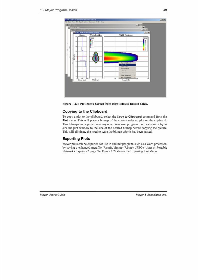
8/20/2019 MFRAC User's Guide
http://slidepdf.com/reader/full/mfrac-users-guide 87/1019
Meyer User’s Guide Meyer & Associates, Inc.
1.9 Meyer Program Basics 3
Figure 1.23: Plot Menu Screen from Right Mouse Button Click.
Copying to the ClipboardTo copy a plot to the clipboard, select the Copy to Clipboard command from thePlot menu. This will place a bitmap of the current selected plot on the clipboard.This bitmap can be pasted into any other Windows program. For best results, try tosize the plot window to the size of the desired bitmap before copying the picture.This will eliminate the need to scale the bitmap after it has been pasted.
Exporting PlotsMeyer plots can be exported for use in another program, such as a word processor,
by saving a enhanced metafile (*.emf), bitmap (*.bmp), JPEG (*.jpg) or Portable Network Graphics (*.png) file. Figure 1.24 shows the Exporting Plot Menu.

8/20/2019 MFRAC User's Guide
http://slidepdf.com/reader/full/mfrac-users-guide 88/1019
40 Getting Started: The Meyer Software
Meyer & Associates, Inc. Meyer User’s Guide
Figure 1.24: Exporting Plot Menu.
It is recommended that metafiles be used whenever possible, since they produce better quality output generally. A metafile is stored as a series of vectors, which can
be scaled to any size, but a bitmap is a fixed size and does not scale well. Portable Network Graphics (*.png) is also scalable. Most figures in this Guide are png files.
To save a plot as a metafile, select Enhanced MetaFile (*.emf) from the Save Fileas Type menu. Then enter a file name for the metafile. This will create a standardwindows metafile of the currently active plot, which can be imported into manygraphics packages and word processors. For example, to insert the metafile intoMicrosoft Word, choose Picture from the Insert menu in Word. Then specify themetafile that was saved from the Meyer program. This will insert the picture intoyour document. Note that the picture can be stretched without losing quality.
Default Plot AttributesThe default plot attributes for all plots can be configured by selecting the DefaultPlot Attributes under the Plot Menu from the Main Menu (see Figure 1.22 ). Thismenu is comprised of the Colors, Fonts and Layout attributes as shown in Figure1.25 .

8/20/2019 MFRAC User's Guide
http://slidepdf.com/reader/full/mfrac-users-guide 89/1019
Meyer User’s Guide Meyer & Associates, Inc.
1.9 Meyer Program Basics 4
Figure 1.25: Default Plot Attributes Menu.
ColorsThe Colors command allows you to specify which colors are used in the plots. The
background, text, frame and grid colors are user specified. By default, all plots usethe colors selected in this box; however, a plot can be configured to have a differentset of colors if desired. For more information on configuring colors, see the PlotConfiguration section below.
General Colors
The default background, text, frame and grid colors are user specified under theGeneral Colors Menu.
To select the default background color click on the color box. A color menu willthen be displayed as shown in Figure 1.26 . Select the color you want and press theOK button.

8/20/2019 MFRAC User's Guide
http://slidepdf.com/reader/full/mfrac-users-guide 90/1019
42 Getting Started: The Meyer Software
Meyer & Associates, Inc. Meyer User’s Guide
Figure 1.26: Default Color Menu.
Curve Attributes
To change the default curve attributes click on the Curve Attributes color box. Thiswill bring up the Line & Curve Attributes dialog box shown in Figure 1.27 .
Figure 1.27: Default Line & Curve Attributes Selection Screen.

8/20/2019 MFRAC User's Guide
http://slidepdf.com/reader/full/mfrac-users-guide 91/1019
Meyer User’s Guide Meyer & Associates, Inc.
1.9 Meyer Program Basics 4
The attributes of a specific line or curve can be modified by clicking on the buttonrepresenting the curve. This will bring up the dialog box shown in Figure 1.27From here the Line Color, Marker Style, Line Style and Line Width can bchanged. Setting the Marker Style to Off turns off the markers for an individualcurve. Likewise, setting the Line Style to Off allows you to plot only the markerswithout lines connecting them. Choosing a Line Width greater than one will take a
longer time to draw the plot.
FontsThe Meyer programs support all True Type fonts installed and available in Win-dows. Clicking on the Font tab will display the font selection screen shown in Figure 1.28 . This will allow you to modify the font and its size.
Figure 1.28: Fonts Selection Screen.
To change the Main Title, X-axis Label, Y-axis Labels, Scale or Legend fonts click on the appropriate selection cell. Figure 1.29 displays the default Plot Font Selec-tion screen. Since font size is always scaled based on the window size, it is impossi-
ble to select an exact point size; however, you may modify the ratio of the font sizeto window size with the Font Size list box.

8/20/2019 MFRAC User's Guide
http://slidepdf.com/reader/full/mfrac-users-guide 92/1019
44 Getting Started: The Meyer Software
Meyer & Associates, Inc. Meyer User’s Guide
Figure 1.29: Default Plot Font Selection Screen.
LayoutFigure 1.30 shows the Default Layout folder which allows you to specify some
basic attributes (Plot Layout, Mouse Coordinates, and Left and Right Axes) used todraw plots. All of these attributes may be overridden in any specific plot by choos-ing the Plot Attributes button in the configuration screen as discussed below.
Figure 1.30: Layout Selection Dialog Box.

8/20/2019 MFRAC User's Guide
http://slidepdf.com/reader/full/mfrac-users-guide 93/1019
Meyer User’s Guide Meyer & Associates, Inc.
1.9 Meyer Program Basics 4
Plot Layout
The different options for determining how the plot is drawn in the window are:
1. Standard plot layout : The plot is always drawn such that the frame has a con-stant aspect ratio, regardless of the size of the window.
2. Maximize plot area : The plot is drawn such that no empty space is wasted. Theaspect ratio of the plot will change as the plot window is sized
3. Allow graphical arrangement : The elements of the plot can be arrangedgraphically. By using the Switch Mouse to Arrange Mode command, the ele-ments of the plot can be manipulated with the mouse. The aspect ratio of the
plot can be user defined.
Mouse Coordinates
The mouse coordinates option allows the coordinates of the current mouse positionto be continuously updated on the screen. When using the graphical plot layoutoption, the coordinates may be positioned anywhere in the window. The coordi-nates are drawn using the same font as the labels on the axes. To view mouse coor-dinates of multi-axes plots place the mouse cursor on the existing mousecoordinates, click the right mouse button and select the desired curve. Figure 1.3illustrates the mouse button selection dialog box.

8/20/2019 MFRAC User's Guide
http://slidepdf.com/reader/full/mfrac-users-guide 94/1019
46 Getting Started: The Meyer Software
Meyer & Associates, Inc. Meyer User’s Guide
Figure 1.31: Mouse Coordinate Selection.
Left and Right Axes
There are four options for how the curves of an axis (left or right) are drawn on the plot. These options are 1) default, 2) like curves share an axis, 3) all curves drawnon one axis, and 4) each curve has its own axis. Figure 1.32 illustrates the case of all curves drawn on one axis. Figure 1.33 shows a plot where each curve has itsown axis. When they each have their own scale, there are labels for each curvealong the axis. The order of the curves in the legend is the same order of the labelson the axis. This option is most useful when there are different kinds of parameterson the same axis, for example rate and concentration.

8/20/2019 MFRAC User's Guide
http://slidepdf.com/reader/full/mfrac-users-guide 95/1019
Meyer User’s Guide Meyer & Associates, Inc.
1.9 Meyer Program Basics 4
Figure 1.32: Axes Label – All Curves on One Axis with Maximize Area.

8/20/2019 MFRAC User's Guide
http://slidepdf.com/reader/full/mfrac-users-guide 96/1019
48 Getting Started: The Meyer Software
Meyer & Associates, Inc. Meyer User’s Guide
Figure 1.33: Axes Label – Each Curve has Its Own Axis.
Slope LinesThe Slope Lines section, as seen in Figure 1.34 , contains global preferences for the
behavior of plot slope lines.
1. The Show Balloon tip checkbox determines whether or not a balloon tip will be displayed while hovering over or moving a plot slope line.
2. The Show ghost line checkbox determines whether or not a temporary line(a.k.a. ghost line) will be drawn while plot slope lines are being moved.

8/20/2019 MFRAC User's Guide
http://slidepdf.com/reader/full/mfrac-users-guide 97/1019
Meyer User’s Guide Meyer & Associates, Inc.
1.9 Meyer Program Basics 4
Figure 1.34: General Plot Slope Line Configuration.
ConfigurationThis will bring up the Plot Configuration dialog box described in detail belowunder Configuring Plots.
Add Text BlockA block of text may be added to any plot by selecting Add a Text Block from thPlot menu or the right mouse button menu as illustrated in Figure 1.35 . Then clicon the plot at the desired location to create a new text block (clicking and draggingallows you to specify the text block width). To edit an existing text block, click on itonce to select it, and again to enter edit mode. Once in edit mode, pressing ENTERwill go to the next line, and CTRL+Z will undo the last change. Press ESCAPE o
click elsewhere in the plot to exit edit mode.

8/20/2019 MFRAC User's Guide
http://slidepdf.com/reader/full/mfrac-users-guide 98/1019
50 Getting Started: The Meyer Software
Meyer & Associates, Inc. Meyer User’s Guide
Figure 1.35: Adding a Text Block to a Plot.
By double clicking on the block, or selecting configuration from the right mouse button menu ( Figure 1.35 ), the attributes of the text block, such as colors, frame,and font, can be configured. Figure 1.36 shows the text block configuration dialog
box. A text block can be deleted by using the right mouse button menu, or pressingDELETE when a text block is selected. The text blocks can also be moved and sizedwith the mouse.

8/20/2019 MFRAC User's Guide
http://slidepdf.com/reader/full/mfrac-users-guide 99/1019
Meyer User’s Guide Meyer & Associates, Inc.
1.9 Meyer Program Basics 5
Figure 1.36: Text Block Configuration.
Zoom OutThis will return the currently selected plot to the previous magnification. For moreinformation on zooming, see the Zoom section above.
Zoom 100%This will return the currently selected plot to the original magnification. For moreinformation on zooming, see the Zoom section above.
Configuring PlotsThe attributes of an open plot may be re-configured by either double-clicking theactive plot in the main plot area or by selecting the Configuration command fromthe Plot menu. This action displays the configuration dialog shown in Figure 1.37
All of these commands are easily accessible at any time by clicking the right mouse button within a plot window.

8/20/2019 MFRAC User's Guide
http://slidepdf.com/reader/full/mfrac-users-guide 100/1019
52 Getting Started: The Meyer Software
Meyer & Associates, Inc. Meyer User’s Guide
Figure 1.37: Plot Configuration Screen.
The Plot Configuration screen provides a method for modifying the text, colors andscales as described in the sections below.
When finished editing the configuration, choose one of the buttons in Table 1.10 toclose the configuration box.
Plot LabelsTo change a plot label, edit the appropriate text in the Plot Labels section at the topof the box. To change the text on the plot legend, see the Legend section below.
Table 1.10: Buttons For Closing Plot Configuration Box.
OK Changes only the current plot in the Plot Configuration screen.
Change Default Applies the changes to this plot and all future plots of the same typethat are plotted, even in different data files.
Cancel Cancels all changes.

8/20/2019 MFRAC User's Guide
http://slidepdf.com/reader/full/mfrac-users-guide 101/1019
Meyer User’s Guide Meyer & Associates, Inc.
1.9 Meyer Program Basics 5
MarkersTurn on the Markers checkbox to see markers on the curve. Fill in the Draw mark-ers every ith point to specify how often to draw markers. For example, a value of two will specify to draw a marker at every other data point. To turn off markers for all curves of the plot, turn this option off. To turn off markers for only selectedcurves of the plot, turn this option on and modify the marker type for the curves onwhich markers are not wanted.
General Sub CategoriesThe sub categories of the General section are shown in Figure 1.38 . This menu icomprised of the Colors, Fonts and Layout attributes.
Figure 1.38: Individual Plot Attributes.
General ColorsOne set of colors, the default colors, is used for all plots. To change these defaultcolors, check the Apply to defaults check box. However, individual plots may havetheir own color scheme.
To use colors other than the defaults, turn off the Use Defaults check box. Then
configure the individual colors by clicking on them, which brings up a palette.Choose the desired color from the palette and click OK . Double-click on the colorsin the palette for quick selection. The definition of the different colors is describedin Table 1.11 .

8/20/2019 MFRAC User's Guide
http://slidepdf.com/reader/full/mfrac-users-guide 102/1019
54 Getting Started: The Meyer Software
Meyer & Associates, Inc. Meyer User’s Guide
Curve AttributesThe attributes of a specific curve can be modified by un-checking the Use Defaults
box and clicking on the box representing the curve. This will bring up the dialogscreen shown in Figure 1.39 . From here the Line Color, Marker Style, Line Styleand Line Width can be changed. Setting the Marker Style to Off turns off the mark-
ers for an individual curve. Likewise, setting the Line Style to Off allows you to plot only the markers without lines connecting them. Choosing a Line Widthgreater than one will slow down the plot drawing process. Clicking Line Color will
bring up the color selection dialog as shown in Figure 1.26 .
To return to the curve defaults, select Use Defaults . From this box, the attributes of any curve can be changed.
Figure 1.39: Line & Curve Attributes Selection Screen.
Table 1.11: Plot General Colors.
Area Definition
BackgroundColor
All the area inside and outside of the plot frame.
Text Color All of the labels, but not the legends (the legends are drawn with thecurve colors).
Frame Color The rectangle that separates the curves from the labels.
Grid Color The grid drawn inside the frame.

8/20/2019 MFRAC User's Guide
http://slidepdf.com/reader/full/mfrac-users-guide 103/1019
Meyer User’s Guide Meyer & Associates, Inc.
1.9 Meyer Program Basics 5
FontsThe Meyer programs support all True Type fonts installed and available in Win-dows. Clicking on the Font tab will display the font selection screen shown in Figure 1.40 . This will allow you to modify the font and its size. Since font size isalways scaled based on the window size, it is impossible to select an exact pointsize; however, you may modify the ratio of the font size to window size with theFont Size list box.
Figure 1.40: Plot Font Selection Screen.
LayoutSee “Layout” on page 44 .
ScalesOn certain plots, it may be desirable to have the X and Y-axes use the same scale.To force them to use the same scale, click on the Scales button in the Plot Control.This will bring up the scales dialog box as shown in Figure 1.41 . Then check X-scales have same Aspect Ratio . To turn off this feature, leave the checkboxunchecked. Only use this feature when the X and Y scales are in the same unit, for example the width contour plot in MFrac . In this plot, the Y scale represents depthand the X scale represents fracture length.

8/20/2019 MFRAC User's Guide
http://slidepdf.com/reader/full/mfrac-users-guide 104/1019
56 Getting Started: The Meyer Software
Meyer & Associates, Inc. Meyer User’s Guide
Figure 1.41: X-Y Aspect Ratio Selection Screen.
Axes
The X and Y axis may be plotted on a linear or log scale. Select Linear or Log asdesired.
The Upper , Lower and Increment may be specified for each axis. The Upper andLower define the range of the scale and the Increment defines how often gridlines,tick marks and numeric labels are drawn. The Increment must be less than theUpper minus the Lower (for positive numbers).
To have the program automatically pick the appropriate settings, check the Autoscale box. This is the default. To manually specify the parameters, turn off theAuto scale box. Note that the X, Y Left and Y Right , and Z axes may be configuredindividually; however the Y Left and Y Right axes share Auto scale and Linear/Log buttons.
To temporarily zoom in on a section of the plot, the Zoom feature as describedabove may be easier to use than manually specifying the scale.

8/20/2019 MFRAC User's Guide
http://slidepdf.com/reader/full/mfrac-users-guide 105/1019
Meyer User’s Guide Meyer & Associates, Inc.
1.9 Meyer Program Basics 5
LegendThe plot legend is used to reference a curve that corresponds or represents a given
parameter. To modify the legend’s attributes, click on the Legend button in the PloAttributes tree view. The Legend Control dialog box for the vertical orientation isshown in Figure 1.42 .
Figure 1.42: Legend Control Dialog Box - Vertical.
To hide the Legend , make sure the Show Legend checkbox is not checked. Toeliminate showing a given curve, enter the Line & Curve Attributes and set bothLine Style and Marker Style to Off.
The legends Show Units option has three radial button choices: 1) Yes - to showthe units, 2) No - do not show units, and 3) Automatic - the code will display unitswhen more than one parameter with different units is present on a given axes. Threeoptions are available for under
The legend Orientation also has three radial button choices: 1) Vertical - the legendwill be placed in the vertical position, 2) Horizontal - the legends will be orientedhorizontally, and 3) Automatic - the legend will be place vertically for a single vari-able on each axes and in the Horizontal position for multiple variables with theoption that each has it’s own axis

8/20/2019 MFRAC User's Guide
http://slidepdf.com/reader/full/mfrac-users-guide 106/1019
58 Getting Started: The Meyer Software
Meyer & Associates, Inc. Meyer User’s Guide
There are five fixed locations for the vertical legend orientation as illustrated inFigure 1.42 , the four corners of the plot and along the right side of the plot. TheLegend Control dialog box for the Horizontal Orientation is shown in Figure 1.43 .There are three locations for the Horizontal legend orientation: 1) Across the Top,2) Position with Mouse, and 3) Across the Bottom.
To allow movement of the legend, anywhere on the screen, select Position withMouse. If Allow graphical arrangement is checked in the Layout dialog box, thelegend can be arranged anywhere on the plot and the Legend Control dialog boxwill be dimmed. Choose the desired location with the corresponding radio button.
Figure 1.43: Legend Control Dialog Box - Horizontal.
To modify the legend font, click on the Fonts button in the tree view. This font can be modified like the label fonts, described above.
To change the legend text, click on the corresponding button at the bottom of thescreen. The left and right buttons allow you to change the text for the curves on theleft and right scales, respectively. After clicking on either of these buttons, a dialog
box will be displayed that contains all of the legends. Modify them as desired andclick OK . To revert to the original legend text, click on the Default button.

8/20/2019 MFRAC User's Guide
http://slidepdf.com/reader/full/mfrac-users-guide 107/1019
Meyer User’s Guide Meyer & Associates, Inc.
1.9 Meyer Program Basics 5
For help with the Multilayer Legend Names section see “Multilayer Legends” on page 207 .
GridlinesTo draw a grid on the plot, click the Gridlines section. The grid is drawn at inter-vals specified by the Increment section of the X and Y-axes. Figure 1.44 shows thgrid selection screen.
Figure 1.44: Grid Selection Screen.
Slope LinesSlope lines can be added to almost any line plot where the x-axis is the independentaxis. Figure 1.45 shows the slope line configuration screen.

8/20/2019 MFRAC User's Guide
http://slidepdf.com/reader/full/mfrac-users-guide 108/1019
60 Getting Started: The Meyer Software
Meyer & Associates, Inc. Meyer User’s Guide
Figure 1.45: Slope Line Configuration Screen.
Each slope line is associated with a left or right curve specified within the CurveNumber column. Toggling the Sync slope and curve colors checkbox synchro-nizes the plot slope line colors to the curve colors.
To manipulate plot slope lines graphically, set the plot mouse mode to Select (pressF4 to toggle between mouse modes). Once in select mode, the slope lines can bemoved by dragging and dropping the points or lines. The plot cursor will changewhen hovering over a slope line to indicate which operation is available.
Color FillWith contour plots, it is possible to show a shaded, color filled or a plain contour
plot. To change this option, click on the Contours button in the Plot Attributes treeview. This will bring up the contour selection screen as shown in Figure 1.46 . Then
choose Shaded, Color Filled Contour, or Plain Contour .

8/20/2019 MFRAC User's Guide
http://slidepdf.com/reader/full/mfrac-users-guide 109/1019
Meyer User’s Guide Meyer & Associates, Inc.
1.9 Meyer Program Basics 6
Figure 1.46: Color Fill Contour Selection Screen.
Shading ColorsThe shading colors are dependent on the Color Fill Contour Selection shown in Figure 1.46 . Figure 1.47 shows the Shaded Contour Color Selection Screen.
Figure 1.47: Shading Colors Selection Screen.
Figure 1.48 shows the Color Filled and Plain Contour Selection Screen. To changea Filled Area Color , click on the color or curve you wish to change. This will bring

8/20/2019 MFRAC User's Guide
http://slidepdf.com/reader/full/mfrac-users-guide 110/1019
62 Getting Started: The Meyer Software
Meyer & Associates, Inc. Meyer User’s Guide
up a dialog box for interactively choosing the color values for Red, Green and Blue.The values must be in the range of 0 to 255.
Figure 1.48: Filled Area Colors Selection Screen.
To return to the defaults for the Filled Area Colors , select Area Color from theDefault section. To make all the Filled Area Colors be shades of a certain color,click on the Shading button and select a base color.
Chart TypeFor chart plots, it is possible to change the chart type. Click on the Chart button inthe Plot Attributes tree view. This brings up the chart dialog as shown in Figure1.49 . Then choose the desired type of plot from the list. The number displayed inthe legend can also be configured. Select either Stage Number, Percentage (percentof total) or Unit Values (the value for the stage).

8/20/2019 MFRAC User's Guide
http://slidepdf.com/reader/full/mfrac-users-guide 111/1019
Meyer User’s Guide Meyer & Associates, Inc.
1.9 Meyer Program Basics 6
Figure 1.49: Chart Type Selection Screen.
Real-TimeMView supports additional configuration for real-time data sets. The Real-Timeconfiguration screen, as seen in Figure 1.50 , is available when an MView plot contains at least one real-time data curve.
Figure 1.50: Real-Time Configuration Screen
The Sliding X Axis option is used to change the auto scaling behavior of the plotsuch that the last X Axis Size units of time are visible within the plot area each timethe plot is rescaled. When the Sliding X Axis option is enabled, the Scale X Axis to
Real-Time option is not available.
The Scale X Axis to Real-Time and Scale Y Axes to Real-Time options modifythe auto scaling behavior of plots that contain both replay and real-time data. To
prevent auto-scaling the X axis according to the replay data on the plot, enable the

8/20/2019 MFRAC User's Guide
http://slidepdf.com/reader/full/mfrac-users-guide 112/1019
64 Getting Started: The Meyer Software
Meyer & Associates, Inc. Meyer User’s Guide
Scale X Axis to Real-Time option. To prevent auto scaling the Y axes according tothe replay data, enable the Scale Y Axes to Real-Time option.
Plot TemplatesThe current state of all the plots on the screen can be saved into a template file. Thistemplate can then be recalled later to view the same plots again, even for a differentsimulation. This makes it easy to recall groups of plots that are always viewedtogether. Any template that is saved can be added directly on the Template menufor easy access.
The template contains the current plot default attributes, identifies opened plots andrelative window positions, and the plot configuration for each of these open plots.Any options associated with these plots (e.g., plotted versus time or volume) arealso saved.
To Save a TemplateOnce the windows are arranged properly, select Save Template from the Template
pop-up menu that is under the Plot menu as shown in Figure 1.51 .

8/20/2019 MFRAC User's Guide
http://slidepdf.com/reader/full/mfrac-users-guide 113/1019

8/20/2019 MFRAC User's Guide
http://slidepdf.com/reader/full/mfrac-users-guide 114/1019
66 Getting Started: The Meyer Software
Meyer & Associates, Inc. Meyer User’s Guide
To Recall a TemplateIf the template is listed on the Template menu, just select it. Otherwise, select LoadTemplate from the Template menu. Then specify the template file. The plots savedin the template will appear.
Organize Template MenuThe Organize Template Menu screen allows for user customization of the Templatemenu. Any template that has been saved may be added to the Template menu for easy access as shown in Figure 1.53 . Within this screen, the templates and the order in which they appear in the menu can be configured.
Figure 1.53: Plot Template Menu Organization Screen.
Figure 1.53 shows the current configuration of the menu, the template descriptionand file location.
To add a template Click on the Add button and select the desired template file. Todelete a Template select the desired template in the list. Then click on the Delete
button. To Move a Template Up in the list select the desired template and click onthe Up button as many times as needed. To Move a Template Down in the list selectthe desired template and click on the Down button as many times as needed.
Click on the OK button after the menu has been configured.

8/20/2019 MFRAC User's Guide
http://slidepdf.com/reader/full/mfrac-users-guide 115/1019
Meyer User’s Guide Meyer & Associates, Inc.
1.9 Meyer Program Basics 6
Run Menu for Other Meyer Applications
Figure 1.54 shows the Run Menu for other Meyer Applications. Simply click on theMeyer Application you wish to execute.
Figure 1.54: Run Menu for Other Meyer Applications.
Simulation Data Windows
Simulation Data Windows (Figure 1.55 ) are available in all of the applications thatcontain a simulator. An application can be identified as having a simulator if thereis a Run item in the main application menu. The Simulation Data Windows provide a read only view of the simulation output data while the simulator is running,and after it has finished running. The data columns within these windows can berearranged or hidden as desired ( See “Spreadsheets With Movable Columns” on
page 31 )

8/20/2019 MFRAC User's Guide
http://slidepdf.com/reader/full/mfrac-users-guide 116/1019
68 Getting Started: The Meyer Software
Meyer & Associates, Inc. Meyer User’s Guide
Figure 1.55: Simulation Data Windows.
Right clicking on any of the Simulation Data Window spreadsheets will display acontext menu providing additional options. To reset the Simulation Data Windowcolumns to their original positions and original visibility, select Restore DefaultColumn Layout from the spreadsheet context menu.
To open a Simulation Data Window at any time, the Show Simulation Data Win-dows sub menu under Plots provides a full list of available windows and a user interface for opening or closing more than one window at a time.
The Simulation Data Windows are magnetic, when a data window is moved or sized too close to another magnetic window, the two windows will ‘snap’ together.To override this feature, hold the CTRL key while sizing or moving the SimulationData Windows .

8/20/2019 MFRAC User's Guide
http://slidepdf.com/reader/full/mfrac-users-guide 117/1019
Meyer User’s Guide Meyer & Associates, Inc.
1.9 Meyer Program Basics 6
When the simulation is started, various Simulation Data Windows are openedaccording to the current Run Options described in the next section.
Run Options
The Run Options dialog box is shown in Figure 1.56 and is available in all applica-tions that contain simulators. To open the Run Options dialog, choose Options...from the Run menu. These options are used during the program execution (Run-ning) and provide flexibility for auto scaling of plots, beeping after each iterationand min./max. error checking.
Figure 1.56: Run Options Dialog Box.
Simulation Data Windows are magnetic; they will snap together if they get closeto one another. Holding the CTRL key overrides this feature.

8/20/2019 MFRAC User's Guide
http://slidepdf.com/reader/full/mfrac-users-guide 118/1019
70 Getting Started: The Meyer Software
Meyer & Associates, Inc. Meyer User’s Guide
Display the following data windows when the sim-ulator is runWhen the simulator is run, the selected windows are automatically opened. This
preference is ignored if the ‘Show template before running simulation’ option ischecked.
Scale plots based on the last run while calculatingWhen running a simulation, all open plots are automatically updated each time step.Since most output parameters are growing during the simulation, this causes the
plot scales to change. Use this option to prevent the scale from changing so often.During a simulation, if the option is on, the plots will automatically use the scale of the last simulation. If an output parameter goes beyond the scale of the last simula-tion, the plots will then automatically rescale. It is advised to leave this option on.
Beep after each time stepIf desired, MFrac can provide audio feedback on the progress of the calculations bygenerating a system beep for each time step. This may be desirable for complicatedsimulations when the calculation times are long. To use this feature click the Beepafter each time step check box.
Disable MIN MAX error checkingThis will disable error checking. Error checking ensures that all input parametersare within the minimum and maximum allowable range when starting a simulation.
Use this option if you have elected to enter a value that is out of range, by clickingon the Ignore button. Otherwise, it is advisable to keep this option off.
Show template before running simulator The current state of all the plots on the screen can be saved into a template file. Thistemplate can then be recalled later to view the same plots again, even for a differentsimulation.
Any template that is saved can be shown during running by selecting the Templatefile using the browse button (The button containing an ellipse; see Figure 1.56 ).
See “Plot Templates” on page 64 for additional information.

8/20/2019 MFRAC User's Guide
http://slidepdf.com/reader/full/mfrac-users-guide 119/1019
Meyer User’s Guide Meyer & Associates, Inc.
1.9 Meyer Program Basics 7
Generating Reports
All of the Meyer programs can generate reports which can be viewed on the screenor exported to a file.
Viewing ReportsTo view a report, choose the View Report command from the Report menu anselect the report type. A report window will then appear. Use the arrow keys or thescroll bars to scroll around the report. The appearance of the report can be config-ured as described below.
Report ConfigurationTo configure the appearance of on-screen reports, select Report Configurationfrom the Report menu. This will bring up the Report Configuration dialog box
shown in Figure 1.57 .
Figure 1.57: Report Configuration Dialog Box.

8/20/2019 MFRAC User's Guide
http://slidepdf.com/reader/full/mfrac-users-guide 120/1019
72 Getting Started: The Meyer Software
Meyer & Associates, Inc. Meyer User’s Guide
To include a bitmap, such as a company logo, at the top of the report, click on theBitmap at top of Report checkbox. Then click on the Select File button to selectthe bitmap file. The bitmap can be left, center or right justified.
There are four different levels of text in reports: the Main Title, Title, Subtitle andMain Text. For each, the justification and font may be configured. Choose the
desired justification with the Left , Center and Right radio buttons. The Main Text justification is not configurable. To select the font for a text level, click on theappropriate Select Font button. From the Font dialog box, select the desired Font,Font style and Size.
The table justification is used to configure how tables are displayed. Select Left ,Center or Right .
To make report windows automatically maximized when they come up, check theAutomatically maximize report windows check box.
Exporting ReportsThere are three options for exporting a report, either as a text, HTML or RTF file. Atext file is formatted by spaces and tabs. An RTF file contains all of the formattingthat is in a report window; however, an RTF file can only be read by word proces-sors that support RTF files.
Save Report as a Text FileTo save a report as a text file, select the text File command from the Report menu.After selecting desired kind of report, enter a file name for the text file.
Save Report as an HTML FileTo save a report as an HTML file, select the HTML command from the Reportmenu. After selecting desired kind of report, enter a file name for the HTML file.
Save Report as an RTF FileTo save a report as an RTF file, select the Save Report as an RTF File commandfrom the Report menu. After selecting desired kind of report, enter a file name for the RTF file.

8/20/2019 MFRAC User's Guide
http://slidepdf.com/reader/full/mfrac-users-guide 121/1019
Meyer User’s Guide Meyer & Associates, Inc.
1.10 Unicode Compatibility 7
1.10 Unicode Compatibility
Overview
As of Meyer 2009, all of the applications included in the Meyer software suite areUnicode compatible. Prior to Meyer 2009, characters were interpreted according tothe Windows “language for non-Unicode programs” setting as seen in Figure 1.58
Figure 1.58: Language for non-Unicode programs.
Pre-Unicode• Characters were represented by a single byte and interpreted according to the
Windows “language for non-Unicode programs” setting.

8/20/2019 MFRAC User's Guide
http://slidepdf.com/reader/full/mfrac-users-guide 122/1019
74 Getting Started: The Meyer Software
Meyer & Associates, Inc. Meyer User’s Guide
• Only 256 distinct characters were representable at a given time.
• Many common symbols could not be used in the user interface due to character encoding limitations.
Unicode• Characters are represented by one or more bytes and interpreted according to
the Unicode standard.
• Thousands of characters are representable depending on available fonts andoperating system compatibility.
• The Windows “language for non-Unicode programs” setting no longer influ-ences how the Meyer applications display characters.
Now that the applications are Unicode compatible, any non-Unicode text loadedfrom a file is converted to Unicode when the file is opened. This applies to most of the file formats that applications prior to Meyer 2009 were capable of saving or exporting. A prompt for choosing an international text encoding will be displayed if this conversion process cannot be completed automatically. An example of this
prompt is show in Figure 1.59 .
Figure 1.59: International Text Encoding Prompt
If a file is opened with an incorrect international text encoding, the text mayappear to be corrupt. If this happens, reopen the file and try choosing a different international text encoding.

8/20/2019 MFRAC User's Guide
http://slidepdf.com/reader/full/mfrac-users-guide 123/1019

8/20/2019 MFRAC User's Guide
http://slidepdf.com/reader/full/mfrac-users-guide 124/1019
76 Getting Started: The Meyer Software
Meyer & Associates, Inc. Meyer User’s Guide

8/20/2019 MFRAC User's Guide
http://slidepdf.com/reader/full/mfrac-users-guide 125/1019
77 Meyer & Associates, Inc.
Chapter 2
MFrac A Three Dimensional HydraulicFracturing Simulator
2.1 IntroductionMFrac is a three-dimensional hydraulic fracturing simulator that is designed to beused as an everyday tool. MFrac accounts for the coupled parameters affecting frac-ture propagation and proppant transport. MFrac is not a fully 3-D model. It is how-ever formulated between a pseudo-3D and full 3-D type model with an applicablehalf-length to half-height aspect ratio greater than about 1/3 (Meyer 15). MFrac alshas options for 2-D type fracture models.
This chapter covers the available menu options and basic procedures required torun MFrac . Please refer to the Meyer Appendices and listed references for specificdetails regarding the governing equations, modeling techniques, methodology andnumerical procedures. Example files are provided with the software to demonstrateMFrac’s features, utility and general data entry procedures.
An outline of the basic steps for using MFrac is shown in Table 2.1 .
Table 2.1: MFrac Basic Steps.
Step Program Area
1. Open an existing MFrac data file (*.mfrac) or create a newdata file.
File Menu
2. Specify Units (optional) Units Menu
3. Select Program Options Data Menu
4. For a real-time or replay case, start MView and import theacquired data.
MView
5. Input Required Data Data Menu

8/20/2019 MFRAC User's Guide
http://slidepdf.com/reader/full/mfrac-users-guide 126/1019
78 MFrac: A Three Dimensional Hydraulic Fracturing Simulator
Meyer & Associates, Inc. Meyer User’s Guide
Menu
The MFrac menu bar is shown in Figure 2.1 . Generally, the menus are accessedfrom left to right with the exception of the Units and Database menus.
Figure 2.1: MFrac Main Menu.
A description of each menu item is described in the following chapters or sectionsas given in Table 2.2 :
6. Run Simulation Run Menu
7. View Plots during or after the simulation Plot Menu
8. Generate Report Report Menu
Table 2.2: Description and Location of Menu Items
Main Menu Item Description Location
File File Management Chapter 1
Options Model Options Section 2.2
Data
DescriptionWellbore Hydraulics
ZonesTreatment ScheduleFoam ScheduleRock propertiesFluid loss DataProppant CriteriaAcid dataHeat Transfer
Section 2.3
Run Start Simulation Section 2.4
Plots Graphical Presentation Section 2.5
Table 2.1: MFrac Basic Steps.

8/20/2019 MFRAC User's Guide
http://slidepdf.com/reader/full/mfrac-users-guide 127/1019
Meyer User’s Guide Meyer & Associates, Inc.
2.2 Options 7
Exporting to Exodus
After the simulation has completed, the propped fracture characteristics may beexported for use with T.T. & Associates Exodus reservoir simulator. To do this,select the Export to Exodus Reservoir Simulator command from the File menu. Ithere is more than one active zone, MFrac will ask which zone to export. Make aselection by choosing the desired zone in the list box and pressing OK . Then MFrawill ask for the file name. Specify the desired file name and press OK . Use this filname when importing data into Exodus.
For more information on the Exodus reservoir simulator, contact T.T. & Associates.
2.2 Options
The Options screen is the first input dialog box under the Data menu in MFrac . It used to establish the primary model options in the program. Each option relates to aspecific aspect of the fracture and proppant/acid modeling approach.
To access the Options screen, select Options from the Data menu by clicking themenu name. The dialog box displayed in Figure 2.2 will then be presented.
Reports Generating Reports Section 2.6
Databases
Fluid DatabaseProppant
Non-Darcy
AcidCasingTubingCoiled-TubingRock Properties
Section 2.7
Table 2.2: Description and Location of Menu Items

8/20/2019 MFRAC User's Guide
http://slidepdf.com/reader/full/mfrac-users-guide 128/1019
80 MFrac: A Three Dimensional Hydraulic Fracturing Simulator
Meyer & Associates, Inc. Meyer User’s Guide
Figure 2.2: Data Options Screen.
The Options screen determines what information is needed for a particular type of analysis. The specific data displayed in a screen or the existence of a data screenitself varies depending on the options selected. This “smart-menu” approach, mini-mizes data input and prevents unnecessary or misleading data entry. Simply decidethe relevant options for a specific simulation and the program will only displaythose menus and input fields necessary. Any time the options are changed the inputdata screens will be updated to enable new input or hide data that is not needed.This hierarchy methodology is used throughout MFrac .
The selections made in the Data Options screen set the scope for all data enteredinto the MFrac program. These options establish the input data required and specifythe nature of the calculations to be performed.
To select an option, click the radio button adjacent to the option preference. A black diamond will then appear in the center of the button selected. Continuing, select aradio button within the next option section or use the TAB button to move sequen-tially through the choices. Once within a section, the current selection for thatoption is highlighted with a dotted rectangle. The option choice may be changed byusing either the mouse or the arrow keys.
General OptionsThe General Options screen allows the user to specify the type of analysis to be per-formed. The choices available for each of the General Options are summarized asfollows:

8/20/2019 MFRAC User's Guide
http://slidepdf.com/reader/full/mfrac-users-guide 129/1019
Meyer User’s Guide Meyer & Associates, Inc.
2.2 Options 8
Simulation MethodDesign ModeThis option is the traditional methodology used for hydraulic fracturing design. The
program flexibility allows for running in standard mode based on a given inputfracture length, slurry volume or treatment schedule. Depending on other optionsspecified, the program uses the formation and treatment data in the calculation of associated fracture and proppant transport characteristics. Design Mode refers tthe fact that the design engineer must design (and optimize) the fracture treatment.
Replay/Real-TimeThe Replay/Real-Time option is required for replaying or performing real-timefracture analysis using the data collected during a treatment. This procedurerequires the use of MView as the real-time or replay data handler. Please refer toChapter 3 for instructions on the use of MView .
With respect to MFrac , there is essentially no difference in the procedures used for performing real-time or replay simulations. The difference between these methodsonly involves the source data input which is handled by MView . Either method permits pressures matching, geometry prediction and proppant transport simulation.
Reservoir CouplingThe mechanisms which control fluid loss from a propagating fracture are discussedin the Appendices. Typically, for general fracturing applications where the leakoff distance perpendicular to the fracture face is small compared to the fracture lengthCarters one-dimensional fluid loss model is adequate. However, for cases with
large fluid loss volumes (e.g., produced water reinjection and large scale frac- packs), the fluid loss behavior is two-dimensional or ellipsoidal. The ellipsoid fluidloss option should be used for cases when the leakoff distance becomes greater thana small fraction of the fracture length.
Linear (Conventional)This is the classic linear fluid loss model as proposed by Carter and assumes thatthe fluid loss is one-dimensional. This option can be used for most applications andis the most common fluid loss model used for propagating fractures.
Ellipsoidal (Koning)This option allows for ellipsoidal (2D) fluid loss from the fracture and generallyresults in lower fracture efficiencies in high permeability formations when largevolumes of fluid are injected. This option requires selection of either the Harmonic

8/20/2019 MFRAC User's Guide
http://slidepdf.com/reader/full/mfrac-users-guide 130/1019
82 MFrac: A Three Dimensional Hydraulic Fracturing Simulator
Meyer & Associates, Inc. Meyer User’s Guide
or Dynamic Fluid Loss Model. The Ellipsoidal model should be selected for pro-duced water reinjection and high permeability large volume frac-packs.
Real-TimeThe Real-Time options are only available if the Replay/Real-Time radio button isclicked On in the Simulation Method dialog. If MView Concentration is selectedthe proppant concentration will be taken from the replay/real-time data as sent toMFrac from MView . If the Input Concentration button is selected the proppantconcentration used by MFrac will be taken from the values specified in the Treat-ment Schedule. Generally, the MView Concentration is desirable unless the actual
proppant concentration injected is not available.
The Synchronize Well Solution radio button is used to synchronize the numeri-cally calculated time steps for wellbore events with the replay/real-time data.
Synchronizing the wellbore solution with the incoming real-time or replay data
enables for very refined calculations of the wellbore and near-wellbore frictional pressure losses. Since the fracture net pressure is not as dependent on the instanta-neous rate changes, this provides the capability to run the fracture model with agreater time step while still simulating the effects of rate changes on frictionallosses in the wellbore and near well region.
Net Present ValueThe Net Present Value option can only be activated if the Simulation Method isDesign Mode .
When the NPV option is turned On , MFrac automatically sets the TreatmentDesign to Auto Design and the Treatment Type to Proppant . For this option, amaximum fracture length is specified in the treatment schedule. MFrac then auto-matically calculates the proppant distribution and fracture conductivity for a num-
ber of incremental fracture lengths up to the maximum value specified. The purpose of this type of analysis is to optimize the design length and conductivity for propped fractures. This process is accomplished by coupling our analytical produc-tion simulator MProd to forecast productivity for each subdivision of the fracturelength. MProd , in turn, produces output used by MNpv to perform Net PresentValue economic optimization calculations.
Turning NPV Off enables the simulator to perform in standard Design, Replay/Real-time or Auto Design mode. This is the general mode of operation unless an NPVanalysis to optimize fracture length is desired.

8/20/2019 MFRAC User's Guide
http://slidepdf.com/reader/full/mfrac-users-guide 131/1019
Meyer User’s Guide Meyer & Associates, Inc.
2.2 Options 8
Fluid Loss ModelThe rate of fluid loss to the formation is governed by the total leakoff coefficient .The three types of flow resistance mechanisms making up are: 1) - leakoff
viscosity and relative permeability effects, 2) - reservoir viscosity and com-
pressibility effects, and 3) - wall building effects.
This option determines which fluid leakoff model is used. The fluid loss modeloptions include specifying the total leakoff coefficient (Constant Model) or the
coefficient and the corresponding components which comprise and (Har-
monic or Dynamic Models). A detailed description of the components characteriz-ing the Harmonic and Dynamic models is given in Appendix D of the Appendicesand in the Fluid Loss Data section of this chapter.
If Constant is selected, the total leakoff coefficient, , is entered in the Fluid Loss
Data screen. The total leakoff and spurt loss coefficients are then input as a functionof depth to characterize fluid loss in the fracture at different intervals.
When either the Harmonic or Dynamic models are chosen, the filter cake coeffi-cient ( ) and reservoir diffusivity parameters are input in the Fluid Loss Data
screen for each layer. The and coefficients are then calculated from the
input reservoir data and fracture propagation characteristics. The total leakoff coef-ficient is then calculated internally as a function of differential pressure.
The weighting of the individual leakoff coefficients for the Harmonic anDynamic models is given in Appendix D.
When the Fluid Type Dependent check box under Fluid Loss Model option ischecked, different total leakoff coefficients (C and Spurt Loss) for each fluid can beentered for the Constant Leakoff model. When the Harmonic or Dynamic Leakoff model is chosen the user can input different wall building coefficients ( ), fil-
trate viscosities, and spurt loss coefficient for each fluid.
This option is useful when large volumes of 2% KCl or treated fluids are in thewellbore prior to pumping the main fracturing treatment. The option is also helpfulfor modeling leakoff during acid fracturing treatments with alternating pad/acid
stages.If the Include Fluid Loss History check box under Fluid Loss Model option ischecked, the simulator will remember the fluid loss history if the fracture closesand then re-opens. This option should be selected to include the effect of the mini-
C
C C I
C II
C II I
C I
C I C II
C
C II I
C I C II
C II I

8/20/2019 MFRAC User's Guide
http://slidepdf.com/reader/full/mfrac-users-guide 132/1019
84 MFrac: A Three Dimensional Hydraulic Fracturing Simulator
Meyer & Associates, Inc. Meyer User’s Guide
frac on the main fracture treatment and when multiple open/close cycles are gener-ated. If this option is checked, the model assumes that the filter cake, viscosity, andcompressibility effects from the previous fracture remain upon re-opening.
Treatment Type
This selection determines the type of fracture treatment. The Treatment Type can be either a propped ( Proppant ) or acid ( Acid ) fracture. In addition, the treatmentcan accommodate an optional foam schedule by checking the Foam box. WhenFoam is checked, MFrac will include compressibility effects.
Treatment Design OptionsThe treatment design options are only available if the Simulation Method is inDesign Mode and the Treatment Type selected is Proppant with no Foam . Thedefault setting is Input for all other cases.
In MFrac , either the pumping schedule can be input manually or determined auto-matically. When Auto Design is chosen, the desired design fracture length or totalslurry volume is input in the treatment schedule dialog box. Depending on theProppant Transport Methodology selected, specific criteria for controlling the
proppant scheduling will also be required.
When Input is chosen, the pumping parameters must be entered into the TreatmentSchedule screen. The exact data input required will depend on selections made for other options (e.g., ramped proppant scheduling, user specified proppant settling,acid fracturing, etc.).
Wellbore Hydraulics ModelThis option determines the wellbore hydraulics model to be used in calculating fric-tional pressure losses in the wellbore. Surface and bottomhole pressures, gravita-tional head, restrictions, transport times and hydraulic power requirements are alsocalculated. The near wellbore and perforation pressure losses are calculated sepa-rately below the BHP reference point for each fracture and coupled to the wellbore.The available wellbore model options are listed below:
When the Net Present Value Option is On the Treatment Schedule Option isautomatically set to Auto Design . For Replay/Real-Time this option is automat-ically set to Input .

8/20/2019 MFRAC User's Guide
http://slidepdf.com/reader/full/mfrac-users-guide 133/1019
Meyer User’s Guide Meyer & Associates, Inc.
2.2 Options 8
NoneWhen this option is selected, wellbore hydraulics calculations are still performed;however, the frictional pressure loss is assumed to be zero. The wellbore hydraulicsoutput data is also not displayed or written to file.
EmpiricalThe Empirical option is an internal correlation for calculating the frictional pres-sure loss of Newtonian and non-Newtonian fluids. This option provides a combinedcorrelation that is applicable for a variety of fluids ranging from linear systems tohighly non-Newtonian and viscoelastic fluids that exhibit drag reduction due to slipor shear thinning during turbulent flow. Three distinct types of behavior are possi-
ble with the combined correlation used in MFrac . These behaviors are illustrated inFigure 2.3 and summarized in the explicit expressions for the Fanning friction fac-tor outlined in Table 2.3
Figure 2.3: Pipe Friction Empirical Correlations.
Table 2.3: Fanning Friction Factors
Maximum Drag Reduction, P.S. Virk 1 (Predicts Minimum Friction)
1 f
----- 19 Re s f log 32.4 – =

8/20/2019 MFRAC User's Guide
http://slidepdf.com/reader/full/mfrac-users-guide 134/1019
86 MFrac: A Three Dimensional Hydraulic Fracturing Simulator
Meyer & Associates, Inc. Meyer User’s Guide
When a value for the Relative Pipe Roughness is entered into one of the WellboreHydraulics dialog boxes, the expression for friction factor based on Prandtl’s “Uni-versal” Law is modified. See Appendix E for additional information.
To include the effects of proppant concentration on friction, the program has a builtin correlation for slurry rheology. The relationship used, originally described byKeck, et al., is also presented in Appendix E.
User DatabaseWhen User Database is selected, the information specified in the fluid database isused for calculating the frictional pressure loss in the tubing, annulus, and casing.This data can be edited and plotted by accessing the database. The information inthe database does not represent proppant-laden fluid. Consequently, if the proppantconcentration wellbore option is selected in the proppant option screen, the frictionfactor will be adjusted for proppant concentration in a manner similar to the methoddescribed in Appendix E for the Empirical option.
Fracture SolutionThese options provide control and flexibility for the time dependent discretizationmethodology used in the program. To enable time step size control for capturingvarious time dependent events, the user can specify the number of fracture Itera-tions and the Maximum Time Step . MFrac will also automatically adjust the timestep size as necessary to control local and global errors. For Replay/Real-Timeanalysis, the data Restart Time can also be specified.
The base time step used for discretization in the numerical simulation will be theminimum of the values calculated from either the number of Iterations or MaxTime Step input.
IterationsThe value for the number of Iterations determines the target number of time stepsto be used for the fracture propagation solution. The total or estimated simulationtime is then divided by the number of iterations to determine the time step size.
Transitional Flow, Keck, et al. 2
No Drag Reduction, Prandtl, et al. 3
(Predicts Maximum Friction)
Table 2.3: Fanning Friction Factors
1 f
----- A Re s f log B+=
1
f ----- 4 Re s f log 0.4 – =

8/20/2019 MFRAC User's Guide
http://slidepdf.com/reader/full/mfrac-users-guide 135/1019
Meyer User’s Guide Meyer & Associates, Inc.
2.2 Options 8
For example, if the number of iterations is 100 and the pump time is 100 minutes,the average time step would be one (1) minute. The actual time step may varydepending on other numerical considerations. For most simulations, a value of 20to 30 iterations is sufficient.
Generally, the number of iterations is most effectively used for design and auto
design. For Replay/Real-Time, the Max Time Step constraint may be more applica- ble.
The number of time steps should be increased for cases with order-of-magnitudechanges in the injection rate or fluid rheology properties (e.g., pad/acid). It shouldalso be increased if the fracture encounters numerous layers in a given time step(especially with diverse properties) or when the injection times are very large (e.g.,years as in water flooding). The maximum time step can also be specified to mini-mize the time step.
If the Alpha Plots accessed from the Fracture Characteristics Plot dialog bo
appear erratic, the number of iterations specified may be too small. Generally, thesolution will not be very sensitive to the number of time steps because of the solu-tion technique used. If the governing equations cannot be solved within a specifictolerance, an alternate solution method is used for that time step. The number of actual fracture solution iterations will always be slightly greater than the valuespecified. The larger this value is, the longer the program will take to run.
Max Time StepThe Max Time Step can be used to control the program time step. This is especiallyuseful when performing real-time or replay simulations. To simulate events thatoccur over a very narrow range of time (e.g., rate changes or pressure spikes) the
time step size must be small enough to capture the event. If the time step is toolarge, significant rate and pressure changes may be missed. Also, the smaller theMax Time Step the longer it will take the program to run.
The Real-Time option of synchronizing the wellbore solution to the input dataenables time refinement for wellbore and near-wellbore pressure losses. This isvery useful for history matching pressure changes due to rate. Also, as stated in theReal-Time options section, the fracture net pressure is a weaker function of ratethan frictional pressure dissipation. This provides the capability to limit the fracturetime step while still maintaining the time refinement necessary to accurately modelwellbore friction.
Restart TimeThe Restart Time is used to start or restart a simulation at a time other than the firstentry point in the data file for real-time or replay simulations. This option is nor-

8/20/2019 MFRAC User's Guide
http://slidepdf.com/reader/full/mfrac-users-guide 136/1019
88 MFrac: A Three Dimensional Hydraulic Fracturing Simulator
Meyer & Associates, Inc. Meyer User’s Guide
mally used when earlier data is not relevant or multiple injection cycles (i.e., mini-frac) are pumped and only the later time cycle data (i.e., main frac) is to beanalyzed. Consequently, this option provides the flexibility to restart a simulation atthe beginning or middle of any injection cycle. Enter the time in the replay/real-time data at which the simulation should begin.
Heat Transfer When turned On , the heat transfer solution can be used to predict the heat-up of thefracturing fluid in the wellbore and the exchange of heat transfer in the fracture tothe reservoir during fracture propagation. The heat transfer solution accounts for conservation of energy and results in simulating the effects of temperature on fluidrheology. The fluid rheology properties as a function of time and temperature arespecified in the Fluid Database.
If heat transfer is turned Off , the in-situ Fluid Temperature is required. The fluidrheological properties are then calculated from the fluid database as a function of
time based on this temperature.
Fracture Options
This group of options is accessed by clicking the Fracture tab found on the DataOptions screen. The Fracture Options provide choices for the fracture geometrymodel and constitutive relationships that affect the fracture solution methodology(see Figure 2.4 ). The choices are as follows:
Figure 2.4: Fracture Options.

8/20/2019 MFRAC User's Guide
http://slidepdf.com/reader/full/mfrac-users-guide 137/1019

8/20/2019 MFRAC User's Guide
http://slidepdf.com/reader/full/mfrac-users-guide 138/1019
90 MFrac: A Three Dimensional Hydraulic Fracturing Simulator
Meyer & Associates, Inc. Meyer User’s Guide
Figure 2.6 shows a vertical ellipsoidal fracture and illustrates the height, width, andlength coordinates.
Figure 2.6: Vertical Ellipsoidal Fracture Geometry.
This model is similar to the Horizontal Ellipsoidal model in appearance only. Themajor differences are related to orientation, intersection effects, influence of in-situstresses, proppant transport and a number of other constitutive relationships.
GDKThe GDK option invokes a constant height fracture geometry model with a verti-cally constant fracture width. That is a vertically unbounded geometry with slip atthe upper and lower extremities as shown in Figure 2.7 . This model is characterized
by a decreasing net pressure with time. This option is most applicable for fractureswith length to height aspect ratios less than unity or for fractureswhich display slip at the upper and lower boundaries. Slip may be an appropriateassumption when rock interfaces are “weak” due to rock competence or when nor-mal stresses may be low (e.g., at shallow depths). The GDK model typically pre-dicts greater wellbore widths and shorter fracture lengths than the PKN model for fractures with aspect ratios greater than unity. The major difference between thePKN and GDK models is in the width-opening pressure relationship as shown
below:
2 L H = 1
GDK - W w pL E PKN - W w pH E

8/20/2019 MFRAC User's Guide
http://slidepdf.com/reader/full/mfrac-users-guide 139/1019
Meyer User’s Guide Meyer & Associates, Inc.
2.2 Options 9
where is the maximum wellbore width, is the half-length, is the height
and is the fracture net pressure.
Figure 2.7: GDK Geometry.
PKNThe PKN model, like the GDK model, is also a constant height model but differs byhaving an elliptically shaped width in the vertical plane (vertically bounded geome-try). Unlike the GDK model, the PKN net pressure increases with time for a con-stant injection rate. The PKN fracture model is most applicable when the totalfracture length is greater than the total fracture height ( ). The major difference between the GDK and PKN model is in the width-opening pressure rela-tionship given above. Figure 2.8 shows the PKN fracture geometry profile.
W w L H
p
2 L H = 1

8/20/2019 MFRAC User's Guide
http://slidepdf.com/reader/full/mfrac-users-guide 140/1019
92 MFrac: A Three Dimensional Hydraulic Fracturing Simulator
Meyer & Associates, Inc. Meyer User’s Guide
Figure 2.8: PKN Geometry.
3-DimensionalThis is a 3-dimensional planar fracture model with both lateral and vertical frac-ture propagation. For large length to height aspect ratios, the model approaches thePKN constant height type geometry. When no confining stress, toughness or mod-uli contrast are entered, the model approaches a vertical radial-type geometry. Thismodel produces the most realistic geometries and is applicable for all length toheight aspect ratios. Figure 2.9 shows a typical 3-Dimensional fracture geometry
profile. As illustrated, the model assumes a bounded geometry at the leading edge(perimeter).
The GDK vertically constant width and PKN elliptical width profiles do not con-trol either models characteristic behavior. It’s all in the width-opening pressure
constitutive relationship. See Meyer 4 for additional comments on model differ-ences.

8/20/2019 MFRAC User's Guide
http://slidepdf.com/reader/full/mfrac-users-guide 141/1019
Meyer User’s Guide Meyer & Associates, Inc.
2.2 Options 9
Figure 2.9: Three-Dimensional Fracture Geometry.
To use a 3-D model effectively, the formation should be characterized sufficientlyto adequately describe the rock and fluid loss properties. To better characterize theformation, the model currently allows up to one thousand (1000) layers for the rock and reservoir properties.
A detailed explanation, formulation and solution methodology for our three-dimen-sional fracturing simulator ( MFrac ) is presented in the appendices.
FlowbackThis option provides the user with the capability to allow fluid and proppant toflowback (negative injection rates and/or cross-flow) from the fracture. To simulatecross-flow between multilayer fractures, this option must be On . If this option iOff , cross-flow during closure and flowback will not be permitted.
This option must be clicked on to simulate flowback, since a negative rate must beinput into the treatment schedule.
Simulate to Closure
When Simulate to Closure is On, the program will simulate closure after pumping.Simulate to closure assumes the spatial fracture compliance factors used during clo-sure remain constant and equal to the values at the end of pumping. This method isless rigorous than the alternative (i.e., when this option is Off ) when closure is sim-ulated with a treatment schedule rate of zero.

8/20/2019 MFRAC User's Guide
http://slidepdf.com/reader/full/mfrac-users-guide 142/1019
94 MFrac: A Three Dimensional Hydraulic Fracturing Simulator
Meyer & Associates, Inc. Meyer User’s Guide
When Simulate to Closure is Off the program will not simulate fracture propagationor lateral proppant transport during closure, unless a zero rate is input in the treat-ment schedule. The proppant transport solution during closure can accommodate
both simulate to closure and a zero rate stage (shut-in) in the treatment schedule.
To maximize compliance precision and propagation accuracy during closure, turn
this option Off and enter a zero rate stage in the Treatment Schedule. Keep in mindthat Simulate to Closure may affect the pressure decline behavior, especially for fractures that grow into multi-stress layers and close with multiple inflection points.
Simulate to closure may not be an appropriate choice for multilayer fractures whichexhibit cross-flow.
Fracture Fluid GradientThis option is only used for the three-dimensional model and allows the user toInclude or Exclude the effect of the fluid gradient on fracture pressure. When
Include is checked, the pressure distribution within the fracture will include thehydrostatic pressure changes as a function of depth (fracture height). The pressuredistribution in turn will affect the fracture propagation.
Normally this option has little effect on the fracture geometry, except for caseswhen the hydrostatic head difference in the fracture is of the same order of magni-tude or greater than the fracture net pressure. This can happen in soft formations(low Young’s modulus) when the fracture height is large.
Propagation ParametersThe options for Propagation Parameters are Default Growth , No Growth During Shut-in , and Positive Growth Only . This option is used to override the propagationrate calculated by the mass conservation, continuity and momentum equations.Fracture propagation will be set to zero during closure if no growth during shut-inis selected. If the Positive Growth Only option is selected the fracture will not beallowed to recede.
These options may be helpful for interference closure, proppant effects, flowback and history matching pressure declines. Low permeability rocks fractured with highefficiency fluids may continue to propagate even after the pumps have shut down.To model the pressure decline the user may want to select Default Growth or Posi-tive Growth Only.
When fracturing wells with large stress contrasts between the reservoir rock and the bounding layers, the upper and/or lower zones may close before the reservoir rock

8/20/2019 MFRAC User's Guide
http://slidepdf.com/reader/full/mfrac-users-guide 143/1019
Meyer User’s Guide Meyer & Associates, Inc.
2.2 Options 9
closes. This will effect the fracture compliance changing the slope of the pressuredecline.
Fracture Initiation IntervalThis option is used to select the manner in which the program initiates the fracture.MFrac , like other fracture models, is a fracture propagation simulator which doesnot simulate the initial formation break down process. Normally for conditionswhere the final fracture geometry is much greater than the initiation geometry, thisinitial boundary condition becomes insignificant in the solution. The choices for fracture initiation are explained below.
Perforated IntervalWhen this option is chosen, the program uses the entire Perforated Interval as thinitial fracture height. The effective closure pressure is then calculated as the mini-mum fracture pressure necessary to keep the fracture open over the perforated inter-
val. This initiation pressure may not be (and usually is not) equal to the minimumhorizontal stress in this interval.
Min. Stress IntervalThe Min. Stress Interval option invokes a routine that uses an initial fracture heightequal to ten (10) percent of the total perforation interval. For this option, the pro-gram examines the formation stress profile and identifies the portion of the perfo-rated interval that contains the zone with the minimum closure pressure required tokeep the fracture open over this limited depth of the perforated interval. This maynot be the interval which contains the lowest minimum horizontal stress. Thisnumerically selected depth interval is then used as the location for fracture initia-
tion.
Fracture Friction Model Normally, laminar flow exists in the fracture and this option may not be needed(i.e., select Off ). For this case, the classical solution for fluid flow in a rectangular slot (as modified for an ellipsoidal fracture width) is used and the Darcy frictionfactor takes the form
where is the Reynolds number ( and )
Deviations from laminar flow affect the frictional dissipation in the fracture and,therefore, on the pressure predicted by a model. Turbulent flow in the fracture may
D 24 Re =
Re Re w = dp dx 1 2 f D2 w – =

8/20/2019 MFRAC User's Guide
http://slidepdf.com/reader/full/mfrac-users-guide 144/1019
96 MFrac: A Three Dimensional Hydraulic Fracturing Simulator
Meyer & Associates, Inc. Meyer User’s Guide
also occur when very low viscosity fluids (e.g., gas) at high rates are pumped. Toaccount for these phenomena and improve the ability to predict non-laminar fric-tional pressure loss in a fracture, the following friction factor expression is usedwhen the Fracture Friction Model is turned On :
Irregularities along the fracture face (e.g., tortuosity, bifuraction and wall rough-ness) that interrupt and disturb fluid flow can also result in greater energy dissipa-tion. These effects can be modeled by increasing the coefficient or modifying thewall roughness factor discussed below.
The approximations for the a and b coefficients in Table 2.4 have been developedempirically in accordance with Prandtl's Universal Law of the Wall (seeSchlichting 3).
Wall RoughnessWhen this option is turned Off , the Darcy friction factor inside the fracture is usedwithout modification as determined from the selections made in the Fracture Fric-tion Model option. This selection assumes that the fracture surface is a smooth pla-nar feature without roughness.
To include the effects of roughness (or waviness) on the frictional dissipation, turn
this option On . This will result in an increase in the frictional pressure drop andfracture width, as well as, a decrease in fracture length. If this option is used, thefriction factor defined in the Fracture Friction Model option will be modified usinga Friction Factor Multiplier. The relationship used is defined in the expressionshown below:
Table 2.4: Typical a and b Friction Coefficients.
Laminar flow Re < 750; a=24; b=1
Transitional flow 750 < Re < 2000; a=0.5; b=0.44
Turbulent flow 2000 < Re < 30,000; a=0.13; b=0.25
Turbulent flow 30,000 < Re < 10 6; a=0.08; b=0.20
Turbulent flow Re > 10 6; a=0.035; b=0.14
MFrac does not use apparent viscosity. The above formulation is based on a power-law Reynolds number to provide the user with insight on the effect of these energy dissipation mechanisms.
Da Re b =
a

8/20/2019 MFRAC User's Guide
http://slidepdf.com/reader/full/mfrac-users-guide 145/1019
Meyer User’s Guide Meyer & Associates, Inc.
2.2 Options 9
where
An empirically derived correlation 5-8 for determining the Friction Factor Multi-plier is shown in Figure 2.10 .
Figure 2.10: Friction Factor Multiplier Empirical Correlation.
Tip EffectsThe observed field pressures for some treatments may at times be much higher thanthe simulated pressure. This discrepancy in measured pressure can be minimized ina number of ways. Typically, the friction factor multiplier, fracture toughness, near-wellbore effects, confining stress or rock/reservoir properties are modified to obtain
= modified Darcy friction factor = Darcy friction factor = friction factor multiplier
D M f f D=
D
D
M f

8/20/2019 MFRAC User's Guide
http://slidepdf.com/reader/full/mfrac-users-guide 146/1019

8/20/2019 MFRAC User's Guide
http://slidepdf.com/reader/full/mfrac-users-guide 147/1019
Meyer User’s Guide Meyer & Associates, Inc.
2.2 Options 9
storage (i.e., if the rate drops suddenly and the BHTP follows, this is not excess pressure but frictional dissipation in the near wellbore region).
Figure 2.11: Fracture Tip Width Reduction due to Non-Linear Elastic Effects.
Proppant Options
This group of options is accessed by clicking the Proppant tab found on the DataOptions screen. The proppant options specify the proppant transport methodologyto be employed. Figure 2.12 illustrates the proppant options available. Theseoptions are discussed below.
The phenomena of tip over-pressure has been referred to as “dilatancy” by someresearchers. It is not clear whether these researchers are referring to rock dilat-ancy or fluid dilatancy. Fluid dilatancy refers to a shear-thickening fluid. Rock
dilatancy describes volumetric expansion of a material that is rapidly approach-ing failure and is usually associated with the micro-cracking process. There hasbeen no published explanation on the effects of rock dilatancy on net pressure ina crack, and to our knowledge, no correlations exist. The desired effect (i.e., anincrease in pressure) can be achieved due to viscosity effects (i.e., fluid dilat-ancy) or as a result of stress dependent rock properties that may or may not berelated to rock dilatancy. This is commonly referred to as nonlinear elasticdeformation. Figure 2.11 illustrates one possibility.

8/20/2019 MFRAC User's Guide
http://slidepdf.com/reader/full/mfrac-users-guide 148/1019
100 MFrac: A Three Dimensional Hydraulic Fracturing Simulator
Meyer & Associates, Inc. Meyer User’s Guide
Figure 2.12: Proppant Options.
Proppant SolutionThe Proppant Solution may be turned On or Off . If Off is chosen, no proppanttransport calculations will be performed and all other options related to the prop-
pant transport will be dimmed. If Off is selected, there will be no coupling betweenthe fracture propagation and proppant transport solutions. Consequently, the frac-ture may propagate backward (negative growth) during closure depending on theR.O.C. of energy and mass conservation. If the proppant transport solution is Onand the Proppant Transport Methodology is not on conventional, negative growthwill not be allowed (this assumes proppant interaction).
When the Proppant Solution option is turned On , proppant transport calculationswill be performed.
If Input is chosen for the Treatment Schedule Options, MFrac calculates the geom-etry and proppant distribution based on the input treatment schedule.
When Auto Design is selected, either the desired fracture length or designed slurryvolume must be entered in the Treatment Schedule screen. The program then auto-matically designs a treatment schedule to satisfy the design criteria. For AutoDesign , the Proppant Type, Initial Proppant Concentration, Incremental Proppant
Concentration, Final Proppant Concentration, Maximum Proppant Concentrationand Proppant Damage Factor must be entered. Depending on the Proppant Trans-port Methodology option selected, the program will internally calculate therequired PAD and proppant schedule to prevent (or create) a screen-out andachieve, if possible, the optimum treatment specified.

8/20/2019 MFRAC User's Guide
http://slidepdf.com/reader/full/mfrac-users-guide 149/1019
Meyer User’s Guide Meyer & Associates, Inc.
2.2 Options 10
Proppant RampThe ramp option controls the ability to ramp the proppant concentration between aspecified range. When this option is On , the concentration of proppant will beramped linearly from an initial value ( From ) to a final ( To ) value for each fluidstage in the Treatment Schedule dialog box. This results in a linear proppant ramp
with liquid volume.
When this option is turned Off , a uniform proppant concentration is assumed for each stage. The Treatment Schedule screen will then permit only one entry valuefor concentration.
Proppant FlowbackThe Proppant Flowback may be turned On or Off . This option when selected Osimulates the flow of proppant back towards the wellbore.
Perforation ErosionThis option allows for perforation erosion during the treatment. If this option isturned On the perforation frictional pressure loss will decrease as the mass of prop-
pant through each perforation increases.
Limited entry designs require a certain differential pressure across the perforationsto ensure that each zone accepts a proportionate amount of fluid and proppant. Dur-ing the limited entry treatment, perforations are exposed to a proppant and liquidslurry. The effect of proppant is to increase the discharge coefficient, , and the
hydraulic diameter of the perforation. The increase in the discharge coefficient can be described as a rounding of the perforation.
Proppant Transport MethodologyThe selection determines how the proppant transport model is linked or coupled tothe fracture propagation calculations. When the Net Present Value option is Onthis option is set to Conventional automatically. The proppant transport methodol-ogy options are: 1) Conventional , 2) Conventional (link proppant ), 3) TiScreen-Out (TSO) , and 4) Frac Pack . With the exception of Conventional , all othe other options couple the proppant transport and fracture propagation solutions.
The TSO and Frac-Pack options are normally used with the Auto Design optionHowever, they are handled the same as the Conventional (link proppant) optiowhen the treatment schedule is Input . The above proppant transport choices are dis-cussed below. Please refer to Appendix I for a detailed description of TSOs andFrac-Packs.
C D

8/20/2019 MFRAC User's Guide
http://slidepdf.com/reader/full/mfrac-users-guide 150/1019
102 MFrac: A Three Dimensional Hydraulic Fracturing Simulator
Meyer & Associates, Inc. Meyer User’s Guide
ConventionalThis option disables the link between the proppant transport and fracture propaga-tion solutions. When this option is selected, the proppant transport calculations willnot affect the fracture propagation behavior. Consequently, for a bridge-out or screen-out the condition of an increasing net pressure will not occur. The proppantcalculations will be performed after each fracture iteration but the results will not
be coupled.
Conventional (Link Proppant)This option links or couples the proppant transport solution with the fracture propa-gation solution to simulate the effects of slurry transport on fracture pressure distri-
bution and propagation. When this option is used, the program will calculateincrementally (i.e., at each time step) a unit of fracture propagation followed by thecorresponding proppant transport time step. If a bridge-out or screen-out conditionoccurs or exists it will affect the pressure distribution in the fracture and subsequentfracture propagation behavior. The resulting change in fracture geometry in turn
influences the overall proppant transport.
When the Auto Design option is used, the choice of Conventional (Link Prop- pant) will cause the program to calculate an optimum proppant transport schedulewithout screening-out. To simulate a TSO or Frac-Pack please refer to one of theoptions described below.
Tip Screen-Out (TSO)This is a specialized form of Meyer & Associates’ proprietary, linked proppantsolution methodology used in MFrac (see Appendix I). The TSO option was specif-ically developed to automatically design a TSO and output the corresponding treat-
ment schedule. This option also couples the proppant transport solution with thefracture solution as does the Conventional (Link Proppant) option when the Treat-ment Schedule Option is on Input . It only differs from the Conventional (Link Proppant) option when the Auto Design feature is used.
Therefore, the following discussion will be directed toward using the TSO option asit pertains to the Auto Design capabilities.
For this option, based on user specified criteria (e.g., target Frac Length, Initial andMax. Inlet Concentration, Average Concentration/Area and Max. BHP), the pro-gram will automatically design a pumping schedule that optimizes a tip screen-out
condition (TSO). Once a screen-out occurs, the net pressure will continue risingduring the remaining part of the treatment to meet the desired design criteria. Dur-ing this type of simulation, the linked solution methodology permits continuous
proppant transport calculations as the slurry is concentrating in the fracture due toleakoff.

8/20/2019 MFRAC User's Guide
http://slidepdf.com/reader/full/mfrac-users-guide 151/1019
Meyer User’s Guide Meyer & Associates, Inc.
2.2 Options 10
The program always satisfies the specified length and then, if possible, the averageconcentration per unit area. User specified constraints are used as absolute limitsand maintain the following priority: Maximum BHP has first priority, Max. Prop-
pant Concentration (lbm/ft 2) in the fracture is second and Maximum Inlet Con-centration is last. If any of the specified criteria are not met, it means that a higher
priority constraint was imposed.
The result is a proppant distribution that approaches a uniform concentration per unit volume throughout the fracture based on the target concentration per unit areaspecified.
Frac-PackThis is a more aggressive variation of the TSO solution technique described above.Once again, it only differs from the Conventional (Link Proppant) option whethe automatic design feature is used.
Like the TSO option, it is also based on the user specified criteria, Frac Length, Ini-tial and Max. Inlet Concentration, Average Concentration/Area and MaximumBHP. When this option is used, the program will automatically determine a pump-ing schedule to first produce a tip screen-out and then pack the fracture. Unlike theTip Screen-out option described above, the Frac-Pack method prevents excessivewidth growth (ballooning) by decreasing the injection rate after the maximum inletconcentration is attained.
The basic premise of this methodology is to control excessive ballooning by match-ing the injection rate to the leakoff rate once the desired geometry is achieved.Please refer to Appendix I for a comparison of the TSO and Frac-Pack Methodolo-gies.
Proppant Settling Options
Four correlations are available for simulating proppant transport and settling 9-12 :
Empirical - lowest settling velocity.
Convective Transport - medium settling velocity.
Cluster Settling - highest settling velocity.
User Specified - user defined settling velocity.
A description of each method is as follows:

8/20/2019 MFRAC User's Guide
http://slidepdf.com/reader/full/mfrac-users-guide 152/1019
104 MFrac: A Three Dimensional Hydraulic Fracturing Simulator
Meyer & Associates, Inc. Meyer User’s Guide
Empirical
This single particle settling velocity correlation is based on the work of Bird, et al. 9
Extension of this work to non-Newtonian fluids for all flow regimes from StokesLaw to Newtonian flow results in the friction factor equations listed below bySlatery 11. The terminology upper and lower bound refers to the coefficient used
in these equations. Wall and slurry concentration (bulk viscosity) effects areincluded in this option to account for hindered settling. These effects are based onmodified density and viscosity correlations.
where
and
Convective TransportThe characteristic dimension that has the most significant influence on the particlesettling velocity for classical ( Empirical ) proppant transport solutions is the particlediameter. Experimental results have demonstrated for certain fluid/proppant combi-nations that this approach, based on modified forms of Stokes Law, significantlyunderestimates vertical settling velocity when large fluid bulk gradients exist.These conditions may occur when large pad volumes, high proppant concentra-tions, or significant stage density contrasts exist.
To account for bulk flow effects, a convective transport correlation is included. Asimplified form of the equation is shown below:
= friction factor = non-Newtonian Reynolds number = 1.1= 0.9= 7.5
Lower Bound 12 ( )
Empirical 9,11
Upper Bound 12 ( )
X
24
Re a--------- 24
Re b--------- X 2 c+ Re 500;=
0.44 500 Re 2.0 x10⁵;=
Reabc
X 3n -1 n 2+3n
--------------n
= X 1
X 1=
X 1 0.8 1 n – 0.7+= X 1

8/20/2019 MFRAC User's Guide
http://slidepdf.com/reader/full/mfrac-users-guide 153/1019
Meyer User’s Guide Meyer & Associates, Inc.
2.2 Options 10
where
The vertical velocity determined from the relationship shown above is corrected for hindered settling using a power law model substitution for apparent viscosity andeffective density approach. The single particle velocity, calculated for an individualstage using the Empirical method described above, is superimposed over the bulk settling solution to characterize the complete settling history of the treatment.
Cluster SettlingLike the convective transport methodology described above, Cluster Settling includes the effects of bulk density gradients and can, therefore, be used to simulategravity induced flow. The formulations developed for this option are given below.The cluster settling rates produced may be higher than convective transport becauseof the differences in the rheology and density corrections used. These correctionsresult in an apparent viscosity that is lower than predicted by convection and aneffective density that is higher. This has the result of reducing the drag or walleffects that are calculated; hence higher settling velocity.
In addition, with Cluster Settling , only the bulk flow is considered. No single par-ticle, Stokes-type settling velocity is included. Consequently, there is no internal
particle settling assumed within an individual cluster.
This correlation may be most applicable when base fluid viscosity is low and prop- pant concentrations are relatively high (e.g., when you are pumping a bankingfluid). The cluster settling formulation is:
where
= vertical (bulk) fluid velocity= fracture width= apparent slurry viscosity
= potential gradient due to gravity, density, and pressure
= vertical (bulk) fluid velocity
v sw2
12 a------------
z =
v s
w
a
z
v s g d eq
2
18a
-------------------=
v s

8/20/2019 MFRAC User's Guide
http://slidepdf.com/reader/full/mfrac-users-guide 154/1019
106 MFrac: A Three Dimensional Hydraulic Fracturing Simulator
Meyer & Associates, Inc. Meyer User’s Guide
and
A power law correlation for apparent viscosity is used for proppant settling.
User Specified SettlingThis option allows the user to input the proppant settling rates manually. Whenselected an additional column or data box will be displayed in the Treatment Sched-ule screen that will allow you to enter a Proppant Settling Rate for each stage. Thevalue entered will be used as a constant rate of settling for that stage.
Wellbore-Proppant EffectsThis option controls the methodology used to simulate the effects of proppant con-centration on pipe friction. The options are as follows:
NoneFor this selection, proppant has no effect on the friction factors used in the wellborehydraulics calculations.
EmpiricalThis option includes the effects of proppant concentration on pipe friction as origi-nally described by Keck, et al. 2 This correlation uses an expression for relativeslurry viscosity to account for the effects of proppant on increased friction. Therelationship is shown below:
= particle diameter = equivalent or characteristic diameter = apparent slurry viscosity= proppant void fraction= packed proppant void fraction
= density difference of particulates and fluid= gravitational acceleration= fracture width
d d eq
a
s
g w
d eq s d w 1 s d – d +=
r 1 0.75 e1.5 n 1 – e 1 n – 1000 – 1.251 1.5 – -------------------+ 2
=

8/20/2019 MFRAC User's Guide
http://slidepdf.com/reader/full/mfrac-users-guide 155/1019
Meyer User’s Guide Meyer & Associates, Inc.
2.2 Options 10
where
For laminar flow, the friction factor multiplier, M, for proppant-laden fluids is equalto the value of . For proppant-laden fluids in turbulent flow, the expression
shown below is used to estimate the effect of proppant on friction:
and
where
User SpecifiedFor some slurry systems, adequate characterization of the frictional dissipation isnot possible with the empirical correlation contained in MFrac . If this occurs, thefriction factor multiplier as a function of proppant concentration can be specified intabular form.
Fracture-Proppant EffectsThis option controls the effect of proppant concentration on frictional pressurelosses in the fracture. The options are summarized below:
= relative slurry viscosity= power-law behavior index for base fluid= Newtonian shear rate= proppant void or particle volume fraction
= friction factor multiplier = base density= relative slurry density;
= slurry density= relative slurry viscosity= friction factor of base fluid= friction factor of slurry
r
n'
r
M f r 0.55
r 0.45=
s M f f b=
M f
b
r r s b =
s
r
b
s

8/20/2019 MFRAC User's Guide
http://slidepdf.com/reader/full/mfrac-users-guide 156/1019
108 MFrac: A Three Dimensional Hydraulic Fracturing Simulator
Meyer & Associates, Inc. Meyer User’s Guide
NoneFor this selection, proppant has no effect on the friction factor calculated in thefracture.
Empirical
This option includes the effects of proppant concentration on fracture friction basedon the empirical expressions shown below. The procedure involves a correction tothe base viscosity to produce a relative viscosity term. Once this is done, the fric-tion factor is calculated based on the Fracture Friction Model selected and theFriction Factor Multiplier (if the Wall Roughness option is activated). The gen-eral correlation as a function of proppant void fraction is:
where
User SpecifiedFor some slurry systems, adequate characterization may not be possible with theempirical correlation contained in MFrac . If this occurs, the friction factor multi-
plier as a function of proppant concentration can be input in tabular form. The val-ues entered are then used to determine the relative viscosity term based on thesolids fraction present. Like in the Wellbore Proppant Effects , the friction factor iscalculated based on the Fracture Friction Model and friction factor multiplier spec-ified (if the Wall Roughness is enabled).
2.3 Data InputOnce the Options are selected the scope of a simulation is set. Data may then beentered by accessing the various dialog boxes from the Data menu. As previouslystated, the option screens determine what information is needed for a particular type of analysis. Consequently, the specific data displayed in a screen or the exis-tence of the data screen will vary depending on the options selected. This approachminimizes data input and prevents unnecessary or misleading data entry. Simplydecide what options are relevant to your simulation and the program will automati-cally display only those menus and input fields necessary. Any time an option ischanged, the input screens will vary to enable new input or hide data that is notneeded. This methodology is used throughout MFrac .
= relative slurry viscosity= exponent coefficient= proppant void or particle volume fraction
r 1 – =
r

8/20/2019 MFRAC User's Guide
http://slidepdf.com/reader/full/mfrac-users-guide 157/1019

8/20/2019 MFRAC User's Guide
http://slidepdf.com/reader/full/mfrac-users-guide 158/1019

8/20/2019 MFRAC User's Guide
http://slidepdf.com/reader/full/mfrac-users-guide 159/1019
Meyer User’s Guide Meyer & Associates, Inc.
2.3 Data Input 11
Injection DownPerforming wellbore hydraulics calculations requires that the wellbore configura-tion and perforations be described. Numerous configurations are possible. Injectioncan be simulated down tubing, casing, annulus or both. To select the configuration,choose one of the radio buttons found in the Injection Down section of the GeneralWellbore Hydraulics screen shown in Figure 2.14 .
The different Injection Down configurations are:
1. Casing - Injection is down the casing. This option assumes there is no tubingin the wellbore. Therefore, tubing data is ignored for this option. If you onlywant to pump down the casing/tubing annulus, check Annulus rather thaCasing .
2. Tubing - Fluid is pumped down the tubing string. When the fluid reaches theend of the tubing it will flow through the casing to the perforations.
3. Coiled Tubing - Fluid is pumped down the coiled tubing. When the fluidreaches the end of the coiled tubing it will flow through the casing to the perfo-rations.
4. Annulus - Fluid is pumped down the annulus between the casing and tubing.Both casing and tubing data must be entered.
5. Tubing and Annulus - For this option, flow will be simulated down both thetubing and annulus. Both tubing and casing data are required for this option.
Horizontal Wells and Frac-Packs
Special wellbore configurations are also available for Horizontal Wells and FracPacks using screen and crossover assemblies. To use one of these configurations,enable the appropriate check box located in the General Wellbore Hydraulicsscreen.
When Horizontal Well is selected, the user can input the MD at the center of the perforations rather than TVD. This provides the capability for locating the perfora-tions on a horizontal section of the casing.
When selecting Frac-Pack Screen , the Screen O.D. and Crossover PressureLoss Coefficient must be entered. This provides the added capability of simulating
flow around the screen (pressure loss) and storage volume reduction due to thedecreased flow area. Once the frac-pack screen diameter is entered it will be dis- played on the wellbore schematic extending from the end of tubing to the end of thecasing. The Crossover Pressure Loss Coefficient is used to calculate the minor
pressure loss associated with the crossover port:

8/20/2019 MFRAC User's Guide
http://slidepdf.com/reader/full/mfrac-users-guide 160/1019
112 MFrac: A Three Dimensional Hydraulic Fracturing Simulator
Meyer & Associates, Inc. Meyer User’s Guide
where
Typical values for the loss coefficient are between two and ten.
Surface Line VolumeThe Surface Line Volume is the volume of fluid/slurry in the service line(s)upstream of the well entrance. Normally this volume is negligible; however, thisline volume may be significant at times (e.g., on Frac Boats). If all the treatment
parameters (rate, volume and staging) are referenced at the well entrance this valueshould be set to zero; however, if all treatment references (measurements and vol-umes) are upstream of the well entrance, this line volume should be specified.
Wellbore Volume Reference DepthThe Wellbore Volume Reference Depth is the depth used for calculating the vol-ume of the wellbore. Either the Measured Depth (MD) or True Vertical Depth(TVD) may be entered. This reference depth must be below the bottom of the tub-ing and above the bottom of the casing. This only applies if there is tubing in thewellbore.
Maximum BHTPThis is the maximum allowable BHTP at the BHTP Reference Depth . If this valueis exceeded during the simulation a warning message will be displayed. This Maxi-mum BHTP is also used as a design criteria in Auto Design mode to ensure that theoptimum design does not exceed this value.
VolumeOn the top of the General tab of the Wellbore Hydraulics dialog box, a Volume isdisplayed. This volume is calculated based on the wellbore configuration andincludes the surface line volume. This volume is also used as the wellbore/flushvolume in the Treatment Schedule.
= pressure loss= loss coefficient= slurry density= velocity
p K s2
2----------- – =
p K
s
v

8/20/2019 MFRAC User's Guide
http://slidepdf.com/reader/full/mfrac-users-guide 161/1019
Meyer User’s Guide Meyer & Associates, Inc.
2.3 Data Input 11
Deviation DataThe first step in describing the wellbore configuration is to enter the wellbore devi-ation survey. To do this, click the Deviation tab found on the Wellbore Hydraulicsdialog box, as shown in Figure 2.15 . A table for wellbore survey stations will then
be displayed.
Figure 2.15: Wellbore Hydraulics - Deviation Tab.
Wellbore Survey MethodThe five standard methods for wellbore survey calculations are supported: AverageAngle, Balanced Tangential, Minimum Curvature, radius of Curvature, and Tan-gential.
Average Angle Method
This method models the well path between two stations as being along a straightline whose length is the measured depth difference between the two stations andwhose inclination and azimuth angles are the average of the stations’ values.

8/20/2019 MFRAC User's Guide
http://slidepdf.com/reader/full/mfrac-users-guide 162/1019
114 MFrac: A Three Dimensional Hydraulic Fracturing Simulator
Meyer & Associates, Inc. Meyer User’s Guide
Balanced Tangential Method
This method models the well path between two stations as two line segments, eachhaving a length that is half the measured depth difference between the stations. Thefirst segment having the inclination and azimuth angles of the first station and thesecond segment have those of the second station.
Minimum Curvature Method
This method is a refinement of the Balanced Tangential Method where the two linesegments are replaced by a circular arc lying in the same plane as the line segments,
but where the arc length is equal to the difference in measured depths of the sta-tions. The implementation is based on the formulation of Sawaryn et al. (see SPE84246)
Radius of Curvature Method
This method models the well path between two stations as a circular arc lying on avertical plane which is then curved along a horizontal circular arc.
Tangential Method
This method, like the Average Angle method, models the well path between twostations as being along a straight line whose length is the measured depth difference
between the two stations, but whose inclination and azimuth are those of the secondstation only.
Deviation InputThe deviation input option determines what data needs to be entered in the devia-tion table. For 3D directional surveys, choose Inclination and Azimuth (3D) (this isthe only option available for the Minimum Curvature method). For 2D inclinationsurveys you have the option of entering the inclination angle or true vertical depth(TVD).
Deviation TableThe table allows input of the wellbore survey stations. It is composed of variouscolumns depending on which input option is selected. For 3D surveys, the mea-sured depth (MD), inclination angle and azimuth angle values are entered, and thenorthing, easting and TVD values are calculated based on the wellbore survey
method selected. For 2D surveys, the table has columns for MD , Inclination Angleand TVD. The input option determines which of the two (inclination angle or TVD)is enter and which is calculated.

8/20/2019 MFRAC User's Guide
http://slidepdf.com/reader/full/mfrac-users-guide 163/1019
Meyer User’s Guide Meyer & Associates, Inc.
2.3 Data Input 11
When using the radius of curvature method, the table includes the Angle BuildRate feature that allows the deviation angle or angle build rate to be specified. If the deviation angle is input, the angle build rate will be calculated. If the angle buildrate is specified the deviation angle will be calculated.
Depths Enter ElsewhereIn several other places, such as the Rock Properties, Fluid Loss, and Zones dialogs,the user can enter depth values in either MD or TVD. This option specifies whichof the two values is keep (while the other is recalculated based on the deviationmodel. This also applies to reference MDs and TVDs on the General and BHTReference tabs in the Wellbore Hydraulics dialog.
When you are finished entering the deviation data, or want to view the data graphi-cally to check its validity, click on the View Deviation Plots button. A dialog boxwill open with a set of tabbed plots: The first is the cross-section that plots the devi-ation’s TVD versus horizontal displacement. The second plots TVD versus MD.The third plots the inclination angle versus MD. For 3D surveys, three addition
plots are included: TVD versus North, TVD versus. East, and North versus. East.
Casing/Tubing DataTo enter pipe data, choose either the Casing and/or Tubing tabs found on the Well-
bore Hydraulics screen, depending upon your application. The program uses theinformation entered to calculate the pipe volume and/or flush volume. The valuecalculated is displayed in the upper left corner of the General Wellbore Hydraulicsscreen and also in the Wellbore section of the Treatment Schedule. Make sure thatthe volume calculated is correct if you are planning to evaluate under- or over-dis-
placement conditions. This is especially important for real-time and replay simula-tion.
For Casing , enter the Measured Depth and Section Length for the portion of thecasing you want to describe ( Figure 2.16 ). Selecting Allow Casing Overlapenables the user to input both the measured depth and section length. If no overlapexists, do not check this box.

8/20/2019 MFRAC User's Guide
http://slidepdf.com/reader/full/mfrac-users-guide 164/1019
116 MFrac: A Three Dimensional Hydraulic Fracturing Simulator
Meyer & Associates, Inc. Meyer User’s Guide
Figure 2.16: Wellbore Hydraulics - Casing Tab.
To specify the OD , ID and pipe Weight , scroll through the Casing Database , found
at the bottom of the Casing screen to locate the correct pipe size. When you havefound the size, click the corresponding database row and the data will automatically
be entered in the casing data table. If the data is not present in the database, it caneither be entered directly in the table or it can be added to the database.
In MFrac , the entry of Casing and Tubing data is handled in a similar manner. For Tubing data, however, it is only necessary to enter the Measured Depth , as nooverlap in sizes is allowed ( Figure 2.17 ). Like the Casing data, once the depthshave been specified, fill in the table with the correct pipe sizes from the TubingDatabase . As each row of data is entered, it is displayed in the wellbore configura-tion diagram located on the left side of the Wellbore Hydraulics screen. The pipe
components and their positions are drawn with the same relative scaling.

8/20/2019 MFRAC User's Guide
http://slidepdf.com/reader/full/mfrac-users-guide 165/1019

8/20/2019 MFRAC User's Guide
http://slidepdf.com/reader/full/mfrac-users-guide 166/1019
118 MFrac: A Three Dimensional Hydraulic Fracturing Simulator
Meyer & Associates, Inc. Meyer User’s Guide
Figure 2.18: Wellbore Hydraulics - Coiled Tubing Tab.
The Total Coiled Tubing Length is the total length of tubing on the reel and in thewell. The Measured Depth is the length of tubing in the well. Length of Coil on theReel is difference between the Total Coiled Tubing Length and the Measure Depth.
The Reel Core Mean Diameter is required input if the User-defined Coiled-TubingReel Friction-Loss Multiplier is unchecked. The friction factor multiplier for thecoil on the reel is then calculated from a modified McCann’s correlation (SPE36345) as given by
where is the fanning friction factor for the coiled-tubing, is the fanning fric-
tion factor for straight tubing, is the coil tubing inside diameter, and is the reelcore diameter (i.e., mean diameter), and the coefficients and are
ct f st 1 a d D b+ =
ct st
d D
a 1.5= b 0.1=

8/20/2019 MFRAC User's Guide
http://slidepdf.com/reader/full/mfrac-users-guide 167/1019
Meyer User’s Guide Meyer & Associates, Inc.
2.3 Data Input 11
representative values. The reel friction multiplier ( , relative to straight tubing) is
given by
If the User-defined Coiled-Tubing Reel Friction-Loss Multiplier is checked, thuser must enter the Reeled-Tubing Friction Loss Multiplier for the coil. Thi
parameter is applied as an additional frictional pressure loss multiplier for the tub-ing on the reel.
In general, the frictional loss multiplier for the tubing on the reel is an additionalmultiplier to the straight tubing friction factor times the straight tubing multiplier.
Pipe roughness is also included in the frictional pressure loss calculation when theWellbore Hydraulics Model is selected as Empirical . When a value is entered forthe Relative Pipe Roughness , the expression used for friction factor is modified in
accordance with Prandtl’s “Universal” law expression. Refer to Appendix E for addition information regarding the effect of wall roughness on the friction factor.
Restrictions DataThe last component included in the wellbore configuration is the description of anyrestrictions that may exist in the tubing. Restriction data is optional and can beentered by clicking the Restrictions tab found on the Wellbore Hydraulics dialog
box as shown in Figure 2.19 . The table that is displayed requires the measureddepth, inside diameter and optional Friction Loss Multiplier for each restrictionThis feature can be used to simulate the effects of various tool or pipe configura-tions.
m
m 1 a d D b+=

8/20/2019 MFRAC User's Guide
http://slidepdf.com/reader/full/mfrac-users-guide 168/1019
120 MFrac: A Three Dimensional Hydraulic Fracturing Simulator
Meyer & Associates, Inc. Meyer User’s Guide
Figure 2.19: Wellbore Hydraulics - Restrictions Tab.
BHTP ReferencesFigure 2.20 shows the BHTP reference depth table. Three (3) BHTP referencedepths can be specified for reporting BHTP in the wellbore. Either the MeasuredDepth (MD) or True Vertical Depth (TVD) may be entered. If the reference depthis above the tubing and you are pumping down both tubing and casing, the BHTP inthe tubing will be reported.

8/20/2019 MFRAC User's Guide
http://slidepdf.com/reader/full/mfrac-users-guide 169/1019
Meyer User’s Guide Meyer & Associates, Inc.
2.3 Data Input 12
Figure 2.20: Wellbore Hydraulics - BHTP References Tab.
ProfileAfter configuring the wellbore components, click the Profile tab on the WellboreHydraulics dialog box to view a graphical representation of the components andwellbore deviation (see Figure 2.21 ). Clicking on the Plot button will open a dialog
box to allow reconfiguring, zooming and printing of the plot.

8/20/2019 MFRAC User's Guide
http://slidepdf.com/reader/full/mfrac-users-guide 170/1019
122 MFrac: A Three Dimensional Hydraulic Fracturing Simulator
Meyer & Associates, Inc. Meyer User’s Guide
Figure 2.21: Wellbore Hydraulics - Profile Tab.
Zones
The Zones dialog box is used to specify the number and location of the perforatedintervals and corresponding Zone Data ( Figure 2.22 ). A maximum of ten different
perforated intervals or limited entry type fractures can be specified. The methodol-ogy and governing equations for multilayer or limited entry fracturing is discussedin Appendix B.
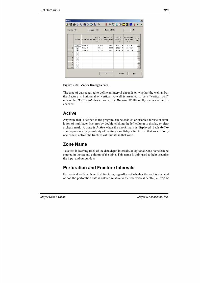
8/20/2019 MFRAC User's Guide
http://slidepdf.com/reader/full/mfrac-users-guide 171/1019
Meyer User’s Guide Meyer & Associates, Inc.
2.3 Data Input 12
Figure 2.22: Zones Dialog Screen.
The type of data required to define an interval depends on whether the well and/or the fracture is horizontal or vertical. A well is assumed to be a “vertical well”unless the Horizontal check box in the General Wellbore Hydraulics screen ischecked.
ActiveAny zone that is defined in the program can be enabled or disabled for use in simu-
lation of multilayer fractures by double-clicking the left column to display or clear a check mark. A zone is Active when the check mark is displayed. Each Activezone represents the possibility of creating a multilayer fracture in that zone. If onlyone zone is active, the fracture will initiate in that zone.
Zone NameTo assist in keeping track of the data depth intervals, an optional Zone name can beentered in the second column of the table. This name is only used to help organizethe input and output data.
Perforation and Fracture IntervalsFor vertical wells with vertical fractures, regardless of whether the well is deviatedor not, the perforation data is entered relative to the true vertical depth (i.e., Top o

8/20/2019 MFRAC User's Guide
http://slidepdf.com/reader/full/mfrac-users-guide 172/1019
124 MFrac: A Three Dimensional Hydraulic Fracturing Simulator
Meyer & Associates, Inc. Meyer User’s Guide
Perfs TVD , Bottom of Perfs TVD ) or measured depths (i.e., Top of Perfs MD , Bot-tom of Perfs MD ).
If a horizontal well is specified in the General Wellbore Hydraulics screen, the cen-ter of the perforated measured depth ( Center of Perfs MD ) is input and the true ver-tical center of the perforated depth ( Center of Perfs TVD ) is calculated. The Center
of Perfs TVD is dimmed and cannot be edited. This same convention is used whenthe Horizontal Ellipsoidal fracture model is specified, even if the well is vertical.
When either the Vertical Ellipsoidal or 3-D geometry options are used in combina-tion with a horizontal well, it is also necessary to enter the TVD for the top and bot-tom of fracture initiation.
When any of the two-dimensional fracture geometry models are chosen from theGeneral Options screen, additional columns of data are required. For the PKN or GDK models, the Zones spreadsheet will contain two additional columns. In thesecolumns you must enter the top true vertical depth of the fracture ( 2-D Top of Frac
TVD) and the bottom true vertical depth of the fracture ( 2-D Bottom of Frac TVD ).This data is used to characterize the total gross height of the fracture. If an Ellipsoi-dal fracture geometry model is chosen, the Ellipsoidal Aspect Ratio must also bespecified. This is the ratio of the major and minor ellipse axes (i.e., the ratio of thetotal length (tip to tip) to the total height of the fracture (2L/H)).
Zone DataAfter entering the Zones perforated depth information, open the Zone Data screenfor each interval by clicking the Edit button found in the far right column. TheZones Data screen shown in Figure 2.23 has tabs for Perforations , Pay Zone , Mul-
tiple Fractures and Near Wellbore . A feature to include perforation erosion is alsoavailable. To activate the perforation erosion folder you must have PerforationErosion selected to User Specified in the Proppant Option Dialog (see Figure2.12).

8/20/2019 MFRAC User's Guide
http://slidepdf.com/reader/full/mfrac-users-guide 173/1019
Meyer User’s Guide Meyer & Associates, Inc.
2.3 Data Input 12
Figure 2.23: Zones Data Dialog Tabs.
Figure 2.23 shows a dimmed perforation erosion table illustrating that Perforation
Erosion was selected to None.
PerforationsFigure 2.24 shows the perforation tab screen. Perforation erosion has been set toUser Specified. This activates the screen for inputting perforation erosion data. The
perforation data requirements are discussed below.

8/20/2019 MFRAC User's Guide
http://slidepdf.com/reader/full/mfrac-users-guide 174/1019
126 MFrac: A Three Dimensional Hydraulic Fracturing Simulator
Meyer & Associates, Inc. Meyer User’s Guide
Figure 2.24: Zone Data - Perforation Tab.
Number and Diameter of Perforations
The Number and Diameter of perforations must also be specified for each perfo-rated zone. These values are entered in the boxes provided at the top of the Perfora-tions screen. This information is used to calculate the perforation friction pressureloss.
Perforation Erosion
The perforation erosion feature is based on the work of Shah 12, Cramer 17, and El-Rabaa, Shah, and Lord 18. This option allows for perforation erosion during thetreatment.
Limited entry designs require a certain differential pressure across the perforationsto ensure that each zone accepts a proportionate amount of fluid and proppant. Dur-ing the limited entry treatment, perforations are exposed to a slurry of proppant andfluid. The effect of the proppant is to increase the discharge coefficient, , andC D

8/20/2019 MFRAC User's Guide
http://slidepdf.com/reader/full/mfrac-users-guide 175/1019
Meyer User’s Guide Meyer & Associates, Inc.
2.3 Data Input 12
the hydraulic diameter of the perforation ( ). The increase in can be
described as a rounding of the perforation.
Figure 2.25 shows the data required to model perforation erosion. To calculate Per-foration Erosion for limited entry fracturing treatments, select Intercept or FinalDischarge Coefficient from the Perforation Erosion dialog box. When Intercept isselected, the intercept is calculated. Enter an Initial Discharge Coefficient , FinaDischarge Coefficient , Perforation Erosion Rate , and Critical Proppant MassWhen Final Discharge Coefficient is chosen enter an Intercept along with the InitialDischarge Coefficient, Perforation Erosion Rate, and Critical Proppant Mass. Thefinal discharge coefficient is then calculated.
Figure 2.25: Perforation Erosion Data Screen.
The discharge coefficient for a sharp-edged perforation entrance is 0.60. For arounded perforation entrance, the discharge coefficient is 0.83. The Final DischargeCoefficient should be set to a larger value than the Initial Discharge Coefficient.
C D1 2/ D C D

8/20/2019 MFRAC User's Guide
http://slidepdf.com/reader/full/mfrac-users-guide 176/1019
128 MFrac: A Three Dimensional Hydraulic Fracturing Simulator
Meyer & Associates, Inc. Meyer User’s Guide
Unless reliable data is available, set the initial value to 0.6 and the Final DischargeCoefficient to 0.83.
Typical values for the Perforation Erosion Rate and Critical Proppant Mass are0.004 in./1000 lbm and 6000 lbm.
To view a plot of the Perforation Erosion correlation, select the Plot icon. Figure2.26 shows a plot of the hydraulic perforation diameter ( ) and pressure loss
ratio as a function of proppant mass through each perforation. The pressure lossratio is the ratio of the perforation pressure loss after proppant has gone throughcompared to the base case of no perforation erosion. As the amount of proppantmass passes through a perforation, the hydraulic diameter increases and the pres-sure loss ratio decreases. After 6000 lbm of proppant has passed through the perfo-
ration, the pressure loss ratio has dropped to less than 60% of its original value.
Figure 2.26: Hydraulic Diameter (C D1/2D) & Pressure Loss vs. Mass.
The upper and lower dashed lines are the theoretical limits for the initial and finalhydraulic perforation diameters. These limits are based on Initial and Final Dis-charge Coefficients of 0.60 and 0.83, respectively.
Note, if perforation erosion is not selected a 0.83 discharge coefficient (i.e.,rounded orifice entrance) is used.
C D1 2/ D
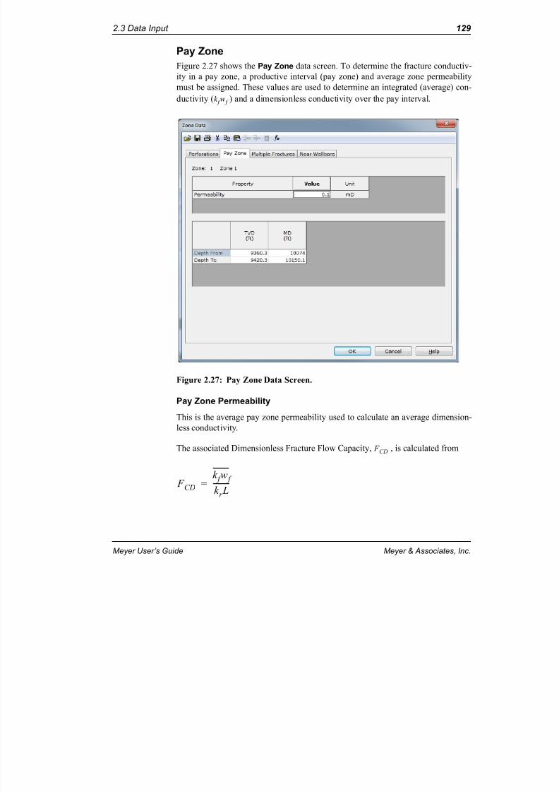
8/20/2019 MFRAC User's Guide
http://slidepdf.com/reader/full/mfrac-users-guide 177/1019
Meyer User’s Guide Meyer & Associates, Inc.
2.3 Data Input 12
Pay ZoneFigure 2.27 shows the Pay Zone data screen. To determine the fracture conductiv-ity in a pay zone, a productive interval (pay zone) and average zone permeabilitymust be assigned. These values are used to determine an integrated (average) con-ductivity ( ) and a dimensionless conductivity over the pay interval.
Figure 2.27: Pay Zone Data Screen.
Pay Zone Permeability
This is the average pay zone permeability used to calculate an average dimension-less conductivity.
The associated Dimensionless Fracture Flow Capacity, , is calculated from
k f w f
F CD
F CDk f w f
k r L---------=

8/20/2019 MFRAC User's Guide
http://slidepdf.com/reader/full/mfrac-users-guide 178/1019
130 MFrac: A Three Dimensional Hydraulic Fracturing Simulator
Meyer & Associates, Inc. Meyer User’s Guide
The average fracture conductivity for long term production is given by
and for short term production or reduced conductivity near the wellbore the follow-ing relationship may be more applicable
where
A more detailed analysis of the effective conductivity for variable conductivityfractures is given in Appendix L.
Pay Zone Depth
A pay zone is defined by entering the TVD or MD Depth From (top) and TVD or MD Depth To (bottom) in the boxes provided. These depths do not have to conform
to the perforated interval. If the fracture is not propped in this interval, the proppedconductivity and propped fracture length will be zero.
Multiple FracturesThis section allows the user to specify the number and degree of interaction of mul-tiple fractures in the specific multilayer zone. This is not the same as multilayer or
limited entry fracturing. Multiple fractures refer to fractures in the far field (notnear wellbore) which may or may not be interacting. These fractures may also be parallel or dendritic (tree like). Figure 2.28 shows the multiple fractures input datascreen.
= average fracture conductivity
= proppant permeability in the fracture
= reservoir permeability= propped fracture width= propped fracture half-length
If the Proppant Transport Plots show a conductive fracture (propped width and conductivity contours) and the pay zone does not appear on the screen or the
pay zone plots show zero conductivity, it indicates that the fracture is not withinthe pay zone.
k f w f k f x w f x xd 0
L L =
k f w f L 1k f x w f x ------------------------- xd
0
L
=
k f w f
k f x
k r w f x
L

8/20/2019 MFRAC User's Guide
http://slidepdf.com/reader/full/mfrac-users-guide 179/1019
Meyer User’s Guide Meyer & Associates, Inc.
2.3 Data Input 13
Figure 2.28: Multiple Fractures Data Screen.
The individual fracture interaction factors and degrees of interaction as given inAppendix C are
Flow Rate
where
Stiffness
where
Fluid Loss
where
Q i qQ t = q 1 N =
E i E E 0= E N 1 – E 1+=
V i V t N =
V t l V 0=

8/20/2019 MFRAC User's Guide
http://slidepdf.com/reader/full/mfrac-users-guide 180/1019
132 MFrac: A Three Dimensional Hydraulic Fracturing Simulator
Meyer & Associates, Inc. Meyer User’s Guide
The interaction factors and degrees of interaction are given by and , respec-tively. The degrees of interaction are the values entered into the program. Theindividual fracture properties and parameters are identified by the subscript i. The
total value for N fractures is given by the subscript t.
Depending on the degree of fracture interaction, the fracture net pressure can belower for multiple fractures than for a single fracture.
If near wellbore multiple fractures are causing near wellbore pressure losses, thenear wellbore pressure loss table should be used.
The reader is referred to Appendix C for additional information regarding multiplefractures and fracture interaction.
Number of Fractures
This is the number of multiple fractures (with two wings) to be modeled in a givenlayer. The default is a single two wing fracture ( Number of Fractures equal toone).
Fracture Interaction
Check this box to specify the degree of stiffness and fluid loss interaction for com- peting fractures. The default is no fracture interaction.
Stiffness Interaction
This represents the per cent of stiffness interaction between the multiple fracturesystem. This parameter can range from 0 to 100%. The interaction values for noand full interaction are zero and 100%, respectively. The closer the fractures aretogether, the greater the stiffness. For multiple parallel fractures within a fraction of their characteristic height, the stiffness increases by a factor equal to the number of fractures (i.e., full interaction). For tree like (dendritic) fractures the stiffness inter-action may be negligible (no interaction).
Fluid Loss Interaction
This represents the percent of fluid loss interaction between the multiple fracturesystem. This parameter can have a value from 0 to 100%. The interaction values for no and full interaction are zero and 100%, respectively. Depending on the reservoir
properties and vicinity of the fracture system, this value may not be the same as thedegree of the stiffness interaction.
l 1 N – l N +=

8/20/2019 MFRAC User's Guide
http://slidepdf.com/reader/full/mfrac-users-guide 181/1019
Meyer User’s Guide Meyer & Associates, Inc.
2.3 Data Input 13
Near Wellbore Pressure TableThe near wellbore pressure loss table is shown in Figure 2.29 . MFrac has the capa
bility to model time and rate dependent near wellbore pressure drop for each frac-ture. This pressure drop can represent any near wellbore effect such as tortuosity,
perforation erosion, near wellbore multiple fractures, etc. The methodologyemployed is explained in Appendix C.
Figure 2.29: Near Wellbore Pressure Loss Screen.
To include the near wellbore pressure drop as a function of time, fill in the spread-sheet located on the right side of the Zone Data screen. Up to fifty rows can bespecified to define the near wellbore pressure drop as a function of time and rate.
Import RT Button
When performing real-time or replay analysis using MView , MFrac automaticallrecords “significant rate and pressure changes” and generates a near wellbore pres-sure loss relationship. After running the acquired data through MFrac , open thZone Data dialog box and choose the Import RT Button . The program will thenload the corresponding data file to fill in the Near Wellbore Pressure Table. If no

8/20/2019 MFRAC User's Guide
http://slidepdf.com/reader/full/mfrac-users-guide 182/1019
134 MFrac: A Three Dimensional Hydraulic Fracturing Simulator
Meyer & Associates, Inc. Meyer User’s Guide
significant rate/BHTP changes were encountered or if the data was not run throughMFrac , a message like the one shown in Figure 2.30 will be displayed.
Figure 2.30: Import RT Message.
The imported near wellbore pressure table includes the total near wellbore pressureloss. This table can be manually changed to incorporate small rate/pressure changesnot considered significant or indeterminate by MFrac .
Once a Near Wellbore Pressure Table has been created, choose how it will beapplied by clicking one of the radio buttons located below the spreadsheet. Theoptions are: to ignore the table completely, use the pressure drop as the total near wellbore effects (including perforations), or to add the resulting effects to the calcu-lated perforation pressure losses (near well effects only).
The program performs a linear interpolation between successive data points for where .If the job duration is longer than the maximum time
entered in the table, the last (final) value will be used
Treatment Schedule
The data required for the Treatment Schedule screen varies depending upon theselections made in the General, Fracture and Proppant Options screens. The smart-menu system used by MFrac only requests the data needed to perform a specificsimulation.
Note for limited entry the imported table must be modified to account for the fractional flow rate going into each fracture.
K t p t K t q t =
K t

8/20/2019 MFRAC User's Guide
http://slidepdf.com/reader/full/mfrac-users-guide 183/1019
Meyer User’s Guide Meyer & Associates, Inc.
2.3 Data Input 13
Auto Design - Treatment ScheduleWhen Auto Design is chosen for the Treatment Schedule Option, a comprehensiveTreatment Schedule screen for auto design is enabled that requires variable inputdepending on the Proppant Transport Methodology (i.e., Conventional, Tip Screen-Out (TSO) or Frac Pack) ( Figure 2.31 ).
The treatment design will be scheduled from the Input Parameter choices of Maxmum Fracture Length , Total Slurry Volume . or Total Proppant Mass . The specific data required will also depend on the selection made for the ProppantDistribution Style Option which allows the user to auto design a treatment sched-ule based on Maximum Proppant Concentration , a specific Concentration per Unit Area , Dimensionless Fracture Conductivity , or Fracture Conductivity the pay zone at closure. An option for the proppant staging profile (staging timefor increasing the proppant concentration using a power law relationship) may also
be selected.
Frac pack designs allow for the additional options for the rate step down during packing, and a rate step down criteria for multi-stage step downs. An option is alsoavailable to maintain a net pressure increase during the rate step down in order to
pack the fracture.

8/20/2019 MFRAC User's Guide
http://slidepdf.com/reader/full/mfrac-users-guide 184/1019
136 MFrac: A Three Dimensional Hydraulic Fracturing Simulator
Meyer & Associates, Inc. Meyer User’s Guide
Figure 2.31: Auto Design Treatment Schedule Screen.
During an auto design simulation, the automatically designed treatment schedule issaved into an output file. This treatment schedule can then be imported into a tabu-lar Treatment Schedule screen ( Auto Design is Off ) for additional editing and sim-ulation using the Import from Output Data button. To use this capability, it isnecessary to run the automatic design case and then change the Treatment Sched-ule Option to Input . This enables the tabular type Treatment Schedule that contains
the Import from Output Data button. Click the button to fill in the TreatmentSchedule table using the data automatically generated by the previous MFrac run.

8/20/2019 MFRAC User's Guide
http://slidepdf.com/reader/full/mfrac-users-guide 185/1019
Meyer User’s Guide Meyer & Associates, Inc.
2.3 Data Input 13
The following input parameters and their descriptions are specific to the AutoDesign Treatment Schedule. Those input parameters not found here are in the sec-tion “Input of Treatment Schedule” below.
Input Parameter MenuThe Input Parameter choices are: Maximum Fracture Length , Total Slurry Vol- ume . or Total Proppant Mass . These choices are available for all Proppant Trans-
port Methodology options including NPV optimization. If a NPV design isselected, designs will be created in increments up to the maximum specified InputParameter value.
Maximum Fracture Length
For an auto design based on fracture length (fracture half-length), a treatmentschedule will be automatically developed to create a fracture length equal to theMaximum Fracture Length input into the dialog.
Total Slurry Volume
The slurry volume is required input when the Auto Design option is based on thetotal slurry volume pumped. The resulting fracture length is then calculated fromthe slurry volume injected.
Total Proppant Mass
The proppant mass is required input when the Auto Design option is based on thetotal proppant mass pumped. The resulting fracture length is then calculated fromthe proppant mass injected and value for the specific Proppant Distribution Styleselected.
Proppant Distribution StyleThe Proppant Distribution Style can have up to four options depending on the Prop-
pant Transport Methodology. If Conventional is selected, the user can specify theauto design proppant scheduling methodology based on 1) The Maximum ProppantConcentration, 2) Concentration per Unit Area, 3) Dimensionless Fracture Conduc-tivity, or the 4) Fracture Conductivity. If the TSO or Frac Pack option is selected,
proppant design scheduling can be based on target values for the Concentration per Unit Area, the Dimensionless Fracture Conductivity, or Fracture conductivity. (i.e.,the Maximum Proppant Concentration option will be dimmed).
If the maximum Proppant Concentration is selected for the Proppant DistributionStyle, the code will design a treatment with the last proppant stage at the final prop- pant concentration. The auto design will create a treatment schedule so that thestages do not screen- or bridge-out and that the maximum proppant concentration inthe fracture will not exceed the maximum value specified in the table.

8/20/2019 MFRAC User's Guide
http://slidepdf.com/reader/full/mfrac-users-guide 186/1019
138 MFrac: A Three Dimensional Hydraulic Fracturing Simulator
Meyer & Associates, Inc. Meyer User’s Guide
The target values for the Concentration per Unit Area, Dimensionless FractureConductivity and Fracture Conductivity are limited by the maximum proppant con-centration pumped. Following are some of the limiting scenarios and numericalresults that will prevent achieving (below or above) the target values for Concentra-tion per Unit Area and/or Conductivity based on the Proppant Transport Methodol-ogy selected in the options screen:
Conventional and Conventional (Link Proppant)
Simulated Concentration per unit Area
Simulated Concentration per unit Area is lower than the specified Target Value.Possible remedies:
• The fracture width is not large enough. Solutions a) Select a TSO or Frac Pack design, b) increase the fluid viscosity, increase the fracture efficiency (decreasefluid loss) or c) Increase the size of the treatment.
• Increase the final proppant concentration.
Simulated Concentration per unit Area is higher than the specified Target Value.Possible remedies:
• Decrease the initial and incremental proppant concentrations.
Simulated Dimensionless Conductivity and Fracture Conductivity
Simulated dimensionless conductivity or conductivity is lower than the specifiedTarget Value. Possible remedies:
• The fracture width is too small. Solutions a) Select a TSO or Frac Pack design, b) increase the fluid viscosity, increase the fracture efficiency (decrease fluidloss) or c) increase the size of the treatment.
• Increase the final proppant concentration.
• Pump a higher permeability proppant.
• The formation permeability may be too high. Therefore the designed fracturelength may be too large for the formation (Dimensionless Conductivity only).
Simulated Dimensionless Conductivity or Fracture Conductivity is higher than thespecified Target Value. Possible remedies:
• Decrease the initial and incremental proppant concentrations.

8/20/2019 MFRAC User's Guide
http://slidepdf.com/reader/full/mfrac-users-guide 187/1019
Meyer User’s Guide Meyer & Associates, Inc.
2.3 Data Input 13
• The propped fracture may be a monolayer. Therefore, design on concentration per unit area.
• Chose a proppant with a lower permeability.
• If in TSO or Frac Pack mode switch to Conventional.
TSO and Frac Pack
Simulated Concentration per unit Area
Simulated Concentration per unit Area is lower than the specified Target Value.Possible remedies:.
• Increase the final proppant concentration and or/increase the maximum allow-able BHTP.
Simulated Concentration per unit Area is higher than the specified Target Value.Possible remedies:
• Decrease the initial and incremental proppant concentrations.
• If TSO is selected change the mode to Conventional. If Frac Pack is selectedchange to TSO.
Simulated Dimensionless Conductivity and Fracture Conductivity
Simulated dimensionless conductivity or fracture conductivity is lower than thespecified Target Value. Possible remedies:
• Increase the final proppant concentration and or/increase the maximum allow-able BHTP.
• Increase the final proppant concentration.
• Pump a higher permeability proppant.
• The formation permeability may be too high. Therefore, the designed fracturelength may be too large for the formation (dimensionless conductivity only).
Simulated dimensionless conductivity or fracture conductivity is higher than thespecified Target Value. Possible remedies:
• Decrease the initial and incremental proppant concentrations.
• The propped fracture may be a monolayer. Therefore, design on concentration per unit area.

8/20/2019 MFRAC User's Guide
http://slidepdf.com/reader/full/mfrac-users-guide 188/1019
140 MFrac: A Three Dimensional Hydraulic Fracturing Simulator
Meyer & Associates, Inc. Meyer User’s Guide
• Chose a proppant with a lower permeability.
• If TSO is selected change the mode to Conventional. If Frac Pack is selectedchange to TSO
Override Internal Concentration Staging Profile
If this option is checked the user can specify the rate of proppant ramping or thechange in proppant concentration with time. The user will also then be asked toinput a Staging Profile Power Law Coefficient. If this box is not checked MFracwill automatically design a treatment schedule based on the minimum, maximum,and maximum concentration at the tip.
Maintain Net Pressure IncreaseThis option is only available for Frac pack designs and if Multi-Stage Step Down isselected. If this box is checked, a treatment design will be calculated to ensure thatthe fracture net pressure does not decrease during the slow down stages. This isaccomplished by designing the slow down rate to always be greater than the leakoff rate. If this option is checked, the user does not have to input the Minimum StepDown Rate.
Fluid TypeWhen clicking or using the TAB key to access a Fluid Type data box, the FluidDatabase pop-up screen is presented allowing the selection of the stage fluid type.Select the desired fluid from the list by clicking on it and the fluid code will auto-matically be entered in the Treatment Schedule. To view the fluid properties for theselected fluid type, click on the Fluid DB button. The specified fluid will be high-lighted in the Fluid Database pop-up screen. Next, press the Edit button to view the
fluid properties.
Proppant TypeWhen a Proppant Type field is entered, either by clicking on it or using the TABkey, the Proppant Database pop-up screen is displayed. Choose the desired prop-
pant type from the list. The proppant code will automatically be entered in theTreatment Schedule. To view the properties that correspond to this proppant code,click on the Proppant DB button. Next, press the Edit button to view the proppant
properties.
Fracture LengthThis input field is only available if the Input Parameter selected is Maximum Frac-ture Length. For an auto design based on fracture length (fracture half-length), thevalue entered will be used to automatically develop a pumping schedule. MFracautomatically determines the required pad and stage volumes to create the input

8/20/2019 MFRAC User's Guide
http://slidepdf.com/reader/full/mfrac-users-guide 189/1019
Meyer User’s Guide Meyer & Associates, Inc.
2.3 Data Input 14
length based on the other parameters entered in the treatment schedule screen.Proppant scheduling is optimized based on the proppant type, concentrations andProppant Transport Methodology option specified.
Total Slurry VolumeThis input field is only available if the selected Input Parameter is Total Slurry Vol-ume. Enter the total slurry to be pumped for the simulation. Based on this volumeand other criteria specified in the Treatment Schedule screen, MFrac will automatically design the pad volume and proppant staging.
Total proppant MassThis input field is only available if the selected Input Parameter is Total ProppantMass. Enter the total proppant mass to be pumped for the simulation. Based on thismass and other criteria specified in the Treatment Schedule screen, MFrac wiautomatically design the pad volume and proppant staging.
Pump RateThis is the slurry rate at which the treatment will be pumped. When performing anautomatic Frac-Pack design, the rate entered is the maximum value that will beused. If the frac pack Rate Schedule option of Single Step Down is selected, MFrawill automatically reduce the rate once the maximum proppant concentration isreached in order to match the leakoff rate and achieve a stabilized fracture pressure.
Minimum Step Down RateThis is the minimum slurry rate at which the treatment will be pumped at the end of the job when performing an automatic Multi-Stage Step Down rate Frac-Pack design. This input parameter is only required if the frac pack Rate Schedule optionof Multi-Stage Step Down Step Down is selected and Maintain net PressureIncrease is not checked., MFrac will automatically reduce the rate once the maxi-mum proppant concentration is reached in order to match the leakoff rate andachieve a stabilized fracture pressure.
Initial and Incremental Prop ConcentrationThis is the initial concentration MFrac will begin automatic scheduling. This valueis also used by MFrac as the step increment for proppant scheduling. In other words, if 2 lb/gal is entered, the proppant concentration will begin at 2 lb/gal for thefirst stage and then proceed with subsequent 2 lb/gal stage increments (i.e., 2, 4, 6,
8.... lb/gal).When the Proppant Ramp option is turned On , this value is used as the initial rampconcentration and increment for staging.

8/20/2019 MFRAC User's Guide
http://slidepdf.com/reader/full/mfrac-users-guide 190/1019
142 MFrac: A Three Dimensional Hydraulic Fracturing Simulator
Meyer & Associates, Inc. Meyer User’s Guide
Final Proppant ConcentrationThis value indicates the final (or last stage) proppant concentration to be pumped
by MFrac . When the Proppant Ramp option is turned On , this value is used as thefinal concentration for the ramp.
Maximum Proppant Concentration (at tip)This value is the maximum volumetric concentration allowed at the fracture tip(e.g., lb/gal) during pumping. It is used as a limit to determine the inlet concentra-tion schedule based on the selection made for the Proppant Transport Methodol-ogy option (i.e., TSO).
All automatic scheduling starts with the Initial Concentration and ends with theFinal Concentration. The Max. Proppant Concentration determines how the pro-gram schedules proppant between these two points.
Target Concentration/Unit Area
The average target concentration per unit area is required input when the ProppantDistribution Style is selected as Concentration per Unit Area. This target parameter may be used when performing a NPV optimization, conventional, automatic tipscreen-out or frac-pack design. Based on this value and the specified Frac Length(or Volume), Initial and Max. Inlet Concentrations, and Max. BHTP, MFrac willautomatically determine a pumping schedule using either the tip screen-out (TSO)or frac-pack criteria selected in the Proppant Transport Methodology option.MFrac always designs to the specified length; and then, if possible, to the averageconcentration per unit area.
The value required by the program is the average mass per unit area of fracture face
(e.g., lb/ft 2) achieved at closure.
Target Dimensionless ConductivityThe Target Dimensionless Conductivity may be input when the Proppant Distribu-tion Style is selected as Dimensionless Conductivity. This input parameter may beused when performing a net present value, conventional, automatic tip screen-outor frac-pack design. Based on this value and the specified Frac Length (or Volume),Initial and Max. Inlet Concentrations, and Max. BHTP, MFrac will automaticallydetermine a pumping schedule based on the selected Proppant Transport Methodol-ogy option. MFrac always designs to the specified length for NPV, Auto Design,TSO and Frac Pack (or volume for conventional); and then, if possible, to the targetdimensionless fracture conductivity in the pay zone as calculated from

8/20/2019 MFRAC User's Guide
http://slidepdf.com/reader/full/mfrac-users-guide 191/1019
Meyer User’s Guide Meyer & Associates, Inc.
2.3 Data Input 14
where is the average conductivity in the pay zone, is the formation permea-
bility, and is the propped fracture length in the pay.
The value required by the program is the target value to be achieved at closure.
Target Fracture ConductivityThe Target Fracture Conductivity may be input when the Proppant DistributionStyle is selected as Fracture Conductivity . This input parameter may be used when
performing a net present value, conventional, automatic tip screen-out or frac-pack design. Based on this value and the specified Frac Length (Volume, or Mass), Ini-tial and Max. Inlet Concentrations, and Max. BHTP, MFrac will automaticallydetermine a pumping schedule based on the selected Proppant Transport Methodol-ogy option. The target fracture conductivity in the pay zone is calculated from
where is the average conductivity in the pay zone, is the variable fracture
conductivity with position in the fracture, and is the propped fracture length in
the pay.
The value required by the program is the target value to be achieved at closure.
Staging Profile Power Law CoefficientThe staging proppant profile power law coefficient is only required input if theOverride Internal Concentration Staging Profile option box is checked. The
proppant concentration as a function of time or volume (for a constant injectionrate) will then be increased (ramped) according to the following formula:
where
= profile power law coefficient= proppant concentration at time
C fDk f w f
kL p---------=
k f w f k
L p
k f w f k f w f x xd 0
L p L p =
k f w f k f w f
L p
c t c t 0 – c t p c t 0 – ------------------------------
t t 0 – t p t 0 – -------------- =
c t t

8/20/2019 MFRAC User's Guide
http://slidepdf.com/reader/full/mfrac-users-guide 192/1019
144 MFrac: A Three Dimensional Hydraulic Fracturing Simulator
Meyer & Associates, Inc. Meyer User’s Guide
The proppant ramp will be linear for , concave upward for , and con-cave downward for . Typical values range from 0.5 to 2.0.
Maximum BHTPThe maximum allowable bottomhole treating pressure is required as a constraintwhen performing automatic tip screen-out or frac-pack designs. Based on this valueand the specified Fracture Length, Initial and Max. Inlet Concentrations, AverageConcentration/Area and target Average Concentration/unit area or target dimen-sionless conductivity, MFrac will automatically determine a pumping scheduleusing the criteria selected in the Proppant Transport Methodology options. Themaximum BHTP is used as a pressure limit to prevent excessive ballooning. If asimulation reaches this constraint before achieving the specified fracture length or
proppant concentration, a message will be displayed indicating that the maximumallowable pressure has been reached. Selecting the message box Cancel button willterminate the simulation. Selecting the OK button will allow you to enter a new
pressure limit.
Input - General Treatment ScheduleIf Input is selected for the Treatment Design Option, a more intuitive Treatment
Schedule is presented. Two tabs are listed under Treatment Schedule, the Generaltab and the Stages tab.
General TabThe General tab for the non-foam Treatment Schedules is shown in Figure 2.32 .
= initial proppant concentration at time
= final proppant concentration at time= time= time of initial concentration or pad= time of final concentration or end of pumping
c t 0 t 0c t p t pt t 0t p
1= 1
1

8/20/2019 MFRAC User's Guide
http://slidepdf.com/reader/full/mfrac-users-guide 193/1019
Meyer User’s Guide Meyer & Associates, Inc.
2.3 Data Input 14
Figure 2.32: Input Treatment Schedule – General Tab.
The General tab contains dialog boxes for Schedule Type and Wellbore .
Schedule Type
In the Schedule Type dialog box select Surface or Bottomhole to specify whethethe data entered (e.g., volumes, rates, etc.) represent surface or bottomhole condi-tions. If pumping from Surface, specify a Wellbore Fluid Type . If pumping fromBottomhole, specify the Flush Fluid Type.
Select Stage Friction Multipliers to enter friction multipliers for each stage.
Select Stage Recirculation to allow the selection of stages, whose rate will be usedto recirculate the fluid that is at bottomhole out of the wellbore.
Wellbore
The wellbore dialog box is related to the initial condition of the wellbore.
Along with the Wellbore Volume displayed from the wellbore hydraulics screen,you can specify a Recirculation Volume . You can also specify whether the well isfilled or partially filled prior to injection. To indicate a partially filled wellbore,enter a fraction (0-1) in the Fraction of Well Filled box. A value of one (1) indi-cates the wellbore is 100% filled. A value of 0.5 means that the well is 50% filled.

8/20/2019 MFRAC User's Guide
http://slidepdf.com/reader/full/mfrac-users-guide 194/1019

8/20/2019 MFRAC User's Guide
http://slidepdf.com/reader/full/mfrac-users-guide 195/1019
Meyer User’s Guide Meyer & Associates, Inc.
2.3 Data Input 14
Figure 2.33: Treatment Schedule – Stages Tab.
To aid in defining the Treatment Schedule, the last column of the table (the VariableColumn) displays a variety of parameters. Use the Variable Column list box tchoose the desired parameter. Depending on the options, the list will contain somesubset of Total Time, Total Liquid Volume, Total Slurry Volume, Total Mass, StageMass, Stage Slurry Volume and Stage Liquid Volume. All of these parameters, withthe exception of the mass parameters, may be modified in the last column. Whenmodifying a total parameter (such as Total Time), changes will be made in the cur-rent stage and the next stage, such that the total parameter for the next stageremains constant. For example, consider the case where Stage 1 has a stage time of 10 and Stage 2 has a stage time of 20. Changing the Total Time of Stage 1 to 15 willcause both Stage 1 and Stage 2 to have stage times of 15.
The treatment schedule table has a few variations that depend on the data options. If the Proppant Ramp option is enabled, additional columns for specifying the rampincrement (i.e., From , To ) are included. Likewise, when the Proppant SettlingModel is User Specified , a column is added to enter the Proppant Settling Rate.
There are other features of the Input Treatment Schedule screen worthy of note.After entering any two of the first three columns, MFrac will automatically calcu-late the third. It is possible to either enter the rate and volume to calculate the time,or enter the rate and time to calculate the volume. In short, MFrac will always guarantee that the rate, time and volume are synchronized.
The following section has a complete list of input parameters and their definitions.

8/20/2019 MFRAC User's Guide
http://slidepdf.com/reader/full/mfrac-users-guide 196/1019
148 MFrac: A Three Dimensional Hydraulic Fracturing Simulator
Meyer & Associates, Inc. Meyer User’s Guide
Recirculate
When the Stage Recirculation option is selected on the General tab, this columnwill appear in the table to allow the selection of stages, whose rate will be used torecirculate the fluid that is at bottomhole, out of the wellbore. For bottomholeschedules, the selected stage is the one that is recirculated out of the wellbore. For surface schedules, it is the fluid that is bottomhole, while the selected stage isinjected at the surface, that is recirculated out of the wellbore.
Slurry Rate
This is the simulated constant rate at which the slurry will be pumped for a specificstage or volume specified. Entering a zero rate and volume is equivalent to specify-ing a shut-in period. For flowback, a negative rate must be specified. The flowback option should be On to enter a negative slurry rate.
Stage Liquid Volume
This is the liquid volume of the stage. In design mode, this is the second column of the treatment schedule table. Since proppant concentration is entered as the mass of
proppant per unit volume of liquid, the calculated pump times displayed include thevolume of the proppant, as well as the liquid (i.e., based on a given slurry rate).
Stage Slurry Volume
This is the slurry volume of the stage. In real-time/replay mode, this is the secondcolumn of the treatment schedule table.
Stage Time
This is the time required to inject the stage slurry volume at the stage slurry rate.When a slurry rate and stage volume are input, the time is automatically calculated.Entering or editing the time for a stage will result in an adjustment to the stage vol-ume.
Stage Type
Figure 2.34 shows the Stage Type in the Treatment Schedule. The stage type optionwas added to clearly identify the type of stage in the treatment schedule. The fol-lowing stage types can be entered in the Treatment Schedule: None (blank), Pre-
pad, Pad, Slug (proppant slug), Prop (proppant), Acid, Flush and Shut-in.

8/20/2019 MFRAC User's Guide
http://slidepdf.com/reader/full/mfrac-users-guide 197/1019

8/20/2019 MFRAC User's Guide
http://slidepdf.com/reader/full/mfrac-users-guide 198/1019
150 MFrac: A Three Dimensional Hydraulic Fracturing Simulator
Meyer & Associates, Inc. Meyer User’s Guide
Fluid Type
When clicking or using the TAB key to access a Fluid Type data box, the FluidDatabase pop-up screen is presented allowing the selection of the stage fluid type.Select the desired fluid from the list by clicking on it and the fluid code will auto-matically be entered in the Treatment Schedule. To view the fluid properties for agiven fluid type either select the corresponding spreadsheet row or wellbore fluidtype and then click on the Fluid DB button. The specified fluid will be highlightedin the Fluid Database pop-up screen. Next, press the Edit button to view the fluid
properties.
Proppant Type
When a Proppant Type field is entered, either by clicking on it or using the TABkey, the Proppant Database pop-up screen is displayed. Choose the desired prop-
pant for the corresponding stage from the list. The proppant code will automatically be entered in the Treatment Schedule. To view the properties that correspond to a proppant code in a given row, click on the Proppant DB button. The specified prop-
pant type will be highlighted in the Proppant Database pop-up screen. Next, pressthe Edit button to view the proppant properties.
Prop. Concentration
When the Proppant Ramp Option is Off , the value entered is a constant for the cor-responding stage. It represents the inlet concentration of proppant per unit volumeof liquid to be injected (mass/volume liquid i.e., lbm/gal liquid). When the Prop-
pant Ramp Option is turned On , the inlet concentration is assumed to increase or decrease as a linear ramp in liquid volume between the From and To values. Thisresults in a uniform increase (or decrease) in proppant concentration with increas-ing liquid volume.
Proppant Damage Factor
The reported final permeability of the proppant in the fracture is calculated from:
where
The bridge-out and screen-out criteria are disabled for Proppant Type 0000independent of the Proppant Transport Methodology option.
= final (damaged) fracture permeability= proppant permeability (undamaged from database)= proppant damage factor
k f k 1 DF – =
k f k
DF

8/20/2019 MFRAC User's Guide
http://slidepdf.com/reader/full/mfrac-users-guide 199/1019
Meyer User’s Guide Meyer & Associates, Inc.
2.3 Data Input 15
The final permeability is used to determine the fracture conductivity and dimen-sionless fracture conductivity.
Proppant Settling Rate
When the User Specified option is chosen for the Proppant Settling Model , thProppant Settling Rate must be entered in the Treatment Schedule. The valueentered will be used as a constant for the settling velocity of the associated proppantstage during the simulation.
Friction Loss Multiplier
To activate the Friction Loss Multiplier column feature, the Stage Friction Multi-plier must be checked in the General tab of the Treatment Schedule dialog box. If stage friction multiplier is checked, friction loss multipliers can be specified for each stage in the Treatment Schedule. This is useful for history matching surfacetreating pressures.
The following explains how the Friction Loss Multiplier is implemented. If thecalculated pipe friction for a stage is 1000 psi and a Treatment Schedule FrictionLoss Multiplier value of 0.85 is entered, the resulting pipe friction would be 850
psi. This multiplier is in addition to the Friction Loss Multiplier in the WellboreHydraulics Screen. Therefore, if the base pressure loss was 1000 psi, and the Fric-tion Loss Multiplier in the Treatment Schedule was 0.85 with a Wellbore Hydrau-lics multiplier of 0.5, the total pressure loss would be 425 psi (1000*0.85*0.5).
Database AccessThe Fluid, Proppant, and Acid Databases can be accessed from the TreatmentSchedule. Figure 2.35 shows accessing the Fluid Database. Once the Fluid Data-
base screen is activated you can add, delete, copy, edit and plot data as if you hadselected the Database menu from the Main Menu tool bar.

8/20/2019 MFRAC User's Guide
http://slidepdf.com/reader/full/mfrac-users-guide 200/1019
152 MFrac: A Three Dimensional Hydraulic Fracturing Simulator
Meyer & Associates, Inc. Meyer User’s Guide
Figure 2.35: Database Access from the Treatment Schedule.
Acid Frac Treatment Schedule
When using the Acid Fracturing option, the treatment schedule replaces the prop- pant scheduling parameters with the required acid fracturing parameters ( Figure2.36). The acid parameters and a brief description of each are given below. Thegeneral treatment parameters of slurry rate, stage volume, etc. are discussed in the“Treatment Schedule Input Parameters” section.

8/20/2019 MFRAC User's Guide
http://slidepdf.com/reader/full/mfrac-users-guide 201/1019
Meyer User’s Guide Meyer & Associates, Inc.
2.3 Data Input 15
Figure 2.36: Acid Treatment Schedule Screen.
Rock/Acid SystemThis five (5) character code identifier specifies which data to use from the AcidFrac Database. The Rock/Acid System database list automatically appears whenthe cursor is placed in this column. Click on the desired rock/acid system from thelist and it will automatically be placed in the column. Moving to any other columncloses the Rock/Acid System list box.
Acid Conc. at InletThis is the acid concentration to be pumped. This value has the units of mass acid/mass liquid (i.e., lbm acid / lbm liquid, or kg acid / kg liquid).
The mass of acid in each stage is calculated and included in the output using the fol-lowing relationship:
where
= mass of acid= inlet acid concentration= stage volume
M a C iV =
M aC iV

8/20/2019 MFRAC User's Guide
http://slidepdf.com/reader/full/mfrac-users-guide 202/1019
154 MFrac: A Three Dimensional Hydraulic Fracturing Simulator
Meyer & Associates, Inc. Meyer User’s Guide
Acid Conc. at EquilibriumThis is the acid concentration below which no reaction with the formation willoccur. This value has the units of mass acid/mass liquid (i.e., lbm acid / lbm liquid,or kg acid / kg liquid).
Diffusivity Multiplier The diffusivity of an acid stage used in a simulation is calculated from the follow-ing:
where
Since the characteristic acid diffusivity is rarely understood, the diffusivity multi- plier is provided as a means of quickly exploring the sensitivity of diffusivity with-out changing the diffusivity permanently in the Rock/Acid database.
Real-Time/Replay Treatment ScheduleWhen using the Replay/Real-Time option, the treatment schedule functions differ slightly from the design table ( Figure 2.37 ). The second column of the table is nowthe Stage Slurry Volume instead of the Stage Liquid Volume. If the Real-Timeoption MView Concentration is selected, the proppant concentration columns inthe treatment schedule will not be editable, since the concentration will be takenfrom the real-time data. If the Input Concentration option is selected, then the con-centration values must be entered in the table. In this case, the Liquid Volumes may
be accessed from the Variable Column.
The most important difference between design and replay/real-time is that the vol-ume and time values are synchronized with the real-time data. This is done auto-matically each time a value is changed. For example, when a stage slurry volume ischanged, MFrac will calculate the total slurry volume up to the end of that stage.Then it will look through the real-time data and find the total time that correspondsto that total volume. The stage time is then calculated from this total time.
The average slurry rates, proppant concentrations and proppant mass for each stageare calculated from the real-time data. These columns are grayed out, since they
= fluid density
= diffusivity used in the fracture
= base diffusivity as given in the database= diffusivity multiplier
D D 0 DM =
D
D0 DM

8/20/2019 MFRAC User's Guide
http://slidepdf.com/reader/full/mfrac-users-guide 203/1019
Meyer User’s Guide Meyer & Associates, Inc.
2.3 Data Input 15
cannot be changed. That is for a specified slurry volume these values are fixed based on the real-time data.
Figure 2.37: Real-Time & Replay Treatment Schedule Screen.
When a stage time is changed, MFrac uses a similar process to calculate a newstage volume. This process insures that the time and volume values are properlysynchronized with the real-time data. If a time or volume value is entered thatcauses a stage to go beyond the real-time data, then the rate column is enabled. Inthis case, the rate, volume and times are synchronized as they are in design mode.To better understand the process of synchronizing with the real-time data, explorethe Graphical Treatment Schedule as described below.
Graphical Treatment SchedulingTo see a graphical picture of the treatment schedule, click on the Graphical TS buton. This will display an interactive plot ( Figure 2.38 ) of Total Slurry Volume vs.Total Time.
This plot allows graphical manipulation of stages. The different stages are repre-sented along the Time and Volume axes by boxes of alternating colors. The alter-nating colors of the Time scale extend through the plot area. Horizontal lines extend
When doing a real-time job, as more data becomes available, the time and ratecolumns may change in order to maintain the proper synchronization. In gen-eral, the slurry volume always takes precedence over time in determining stag-ing.

8/20/2019 MFRAC User's Guide
http://slidepdf.com/reader/full/mfrac-users-guide 204/1019
156 MFrac: A Three Dimensional Hydraulic Fracturing Simulator
Meyer & Associates, Inc. Meyer User’s Guide
from the boxes of the Volume scale to aid in visualizing the stage volumes. Whenusing the Replay/Real-time option, the data in the plot is the real-time data fromMView . The real-time rate is integrated to get the volume curve.
The right axis drop down selection box can now display any parameter sent fromMView (i.e., Rate, Surface Pressure, BHTP, Concentrations etc.).
Figure 2.38: Graphical Treatment Schedule Screen.
Another Graphical Treatment Schedule feature is graphical placement of the restarttime (i.e., the start of the first stage can now be moved like any of the other stages).
Graphical Treatment MenuThe graphical treatment schedule has its own menu bar at the top of the screen.Many of the menu commands are standard Meyer menu commands described inChapter 1. The others are described below:

8/20/2019 MFRAC User's Guide
http://slidepdf.com/reader/full/mfrac-users-guide 205/1019
Meyer User’s Guide Meyer & Associates, Inc.
2.3 Data Input 15
The File Menu
End Editing without making changes
This will end the editing session without keeping any changes made during the edit-ing session.
End Editing
This will end the editing session and keep all changes made.
The Edit Menu
Add Stage
This will add a new stage after the currently selected stage. If the currently selectedstage is last stage, the new stage will have exactly the same properties as the currentstage. If the current stage is not the last stage, it will cut the current stage’s volumein half. The new stage will have the same properties as the current stage, except itwill have one half of the slurry volume. In this case, adding a stage is essentiallysplitting the current stage into two equal stages. A dialog box will allow modifica-tion of the new stage.
Pressing the Insert key will also activate this command.
Delete Stage
This will delete the currently selected stage. The stage numbers of all the subse-quent stages will then decrease by one.
Pressing the Delete key will also activate this command.
Modify Stage
This will allow manual modification of the currently selected stage. A dialog boxthat resembles the treatment schedule table will appear; however, it will only haveone row representing the selected stage. This box functions exactly the same as thenormal treatment schedule with a few exceptions. Changing total values in the Varable Column has no effect on other stages. Any change in stage volume may besubtracted from the previous or next stage as selected with the Previous , Next oNeither buttons. When Neither (the default) is selected, none of the other stage vol-
umes will be affected.Double-clicking the mouse on a stage while in Select mode will also bring up themodify stage box.

8/20/2019 MFRAC User's Guide
http://slidepdf.com/reader/full/mfrac-users-guide 206/1019
158 MFrac: A Three Dimensional Hydraulic Fracturing Simulator
Meyer & Associates, Inc. Meyer User’s Guide
Undo all changes
This will undo all changes made during this editing session.
The Toolbar At the top of the plot is a toolbar. In the top left of the toolbar, the current mouse
location on the X, YL (left), and YR (right) scales is displayed. The End Edit buttoncan be used to end the current editing session. The mouse can be set to Selectstages or Zoom in with the Mouse list box. The Right Axis list box is used tochange which data is plotted on the right axis. The choices are Rate & Concentra-tion, Rate, Concentration or None. The bottom portion of the toolbar displays infor-mation about the currently selected stage.
Modifying Stages GraphicallyThe real power of the graphical treatment plot is the ability to manipulate the stagevolumes and times with the mouse. It is important to understand that there are twodistinct mouse modes, Select and Zoom . The mode can be toggled with the Mouselist box or the right mouse button menu.
When in Zoom mode, the mouse functions as in any other Meyer plot, the leftmouse button can be used to define an area of the plot for zooming.
The Select mode is used for selecting and modifying the active stage. Clicking themouse on any stage will make it the active stage. To graphically change a stage,click and drag on the desired boundary (either time or volume). The stage informa-tion in the toolbar will be updated automatically while dragging the stage boundary.Also note that a boundary cannot be moved past the boundaries on either side of it.The stage before and after a boundary will be modified if the boundary is changed.To keep the stage time (or volume) after the boundary constant, hold down the Con-trol key when dragging the boundary. Then, only the stage before the modified
boundary will change.
When working with a real-time treatment schedule, the times and volumes willautomatically be synchronized to the real-time data. If a stage goes beyond the endof the current real-time data, its box on the X axis will extend to the right edge of the plot. All subsequent stages will not have a box on the X scale; however, allstages will be represented on the Y axis. As more real-time data becomes available,those stages which were previously beyond the end of the data may be in the rangeof available data. In this case, the stage will get a new stage time from MFrac .
When flowback is enabled, all stages after the first stage with a negative rate stagewill not be represented on the Y axis. The volume of these stages may not bemanipulated graphically; however, the time of these stages may.

8/20/2019 MFRAC User's Guide
http://slidepdf.com/reader/full/mfrac-users-guide 207/1019

8/20/2019 MFRAC User's Guide
http://slidepdf.com/reader/full/mfrac-users-guide 208/1019
160 MFrac: A Three Dimensional Hydraulic Fracturing Simulator
Meyer & Associates, Inc. Meyer User’s Guide
Quality
The foam schedule allows for the design of Mitchell, Both External Phase, InternalPhase (CO2), and Internal Phase (N2) foam quality treatments. These qualities areat bottomhole conditions as defined below:
Mitchell
and
Both External Phase
and l
Internal Phase CO2
andl
Internal Phase N2
and l
The foam and total volumes are defined as:
where
= foam quality (void fraction)= carbon dioxide volume
= foam volume= liquid volume
= nitrogen volume= proppant volume= total volume
N 2V N 2
V f = CO 2V CO 2
V f =
N 2V N 2
V t = CO 2V CO 2
V t =
N 2V
N 2V
t =
CO 2V
CO 2V
p+ V
t =
N 2V N 2
V p+ V t = CO 2V CO 2
V t =
V f V N 2V CO 2
V l + +=
V t V f V p+=
V CO 2
V f V l V N 2
V pV t

8/20/2019 MFRAC User's Guide
http://slidepdf.com/reader/full/mfrac-users-guide 209/1019
Meyer User’s Guide Meyer & Associates, Inc.
2.3 Data Input 16
Standard Conditions
Quantities such as N 2 volume & rate and CO 2 solubility are given in units at stan-dard conditions. The user has the following options to indicate the standard condi-tions:
1. 60 °F, 1 atm : The standard conditions are 60 °
F, 1 atm.
2. User Specified : The user specifies the densities for CO 2 and N 2 at standarconditions.
Density
The density option specifies how densities for CO 2 and N 2 at bottomhole and COdensity at the flow meter are determined. The user has the following choices:
1. Van der Waals EOS: Use the van der Waals equation of state.
2. Peng-Robinson EOS: Use the Peng-Robinson equation of state.
3. User Specified: The user specifies the densities directly.
When using an equation of state (EOS) the following information is required:
1. CO2 Pressure (Flow Meter); required if pumping CO2.
2. CO2 Temperature (Flow Meter); required if pumping CO2.
3. BHTP (Bottomhole treating pressure).
4. BHTT (Bottomhole treating temperature).
CO2 Solubility
The carbon dioxide solubility at bottomhole conditions.
Saturated Liquid Volume Ratio
For CO2 in solution, this is the ratio of fully saturated liquid volume to unsaturatedliquid volume.
Stages TabFigure 2.40 shows the Foam Treatment Schedule screen.
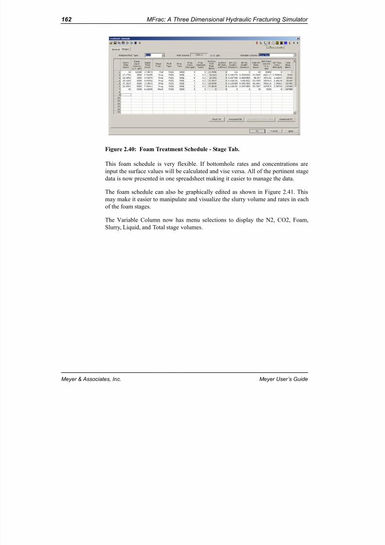
8/20/2019 MFRAC User's Guide
http://slidepdf.com/reader/full/mfrac-users-guide 210/1019
162 MFrac: A Three Dimensional Hydraulic Fracturing Simulator
Meyer & Associates, Inc. Meyer User’s Guide
Figure 2.40: Foam Treatment Schedule - Stage Tab.
This foam schedule is very flexible. If bottomhole rates and concentrations areinput the surface values will be calculated and vise versa. All of the pertinent stagedata is now presented in one spreadsheet making it easier to manage the data.
The foam schedule can also be graphically edited as shown in Figure 2.41 . Thismay make it easier to manipulate and visualize the slurry volume and rates in eachof the foam stages.
The Variable Column now has menu selections to display the N2, CO2, Foam,Slurry, Liquid, and Total stage volumes.

8/20/2019 MFRAC User's Guide
http://slidepdf.com/reader/full/mfrac-users-guide 211/1019
Meyer User’s Guide Meyer & Associates, Inc.
2.3 Data Input 16
Figure 2.41: Foam Schedule - Graphical Editing.
Rock Properties
The Rock Properties dialog box provides a table for entering the mechanical prop-erties of the reservoir and adjacent lithologies including in-situ stresses as a func-tion of depth (see Figure 2.42 ). For each layer an optional Lithology Symbol , anZone Name can be specified to help organize the rock properties table. The TV
depth at the bottom of the zone ( Depth at Bottom ) is the next entry. By convention,this is the true vertical depth (TVD) at the bottom of each zone or layer. The MD aBottom is then calculated from the TVD or if the MD is specified the TVD depthwill be calculated.
Once a zone is defined, after MD at Bottom, the representative, Stress Gradient,Stress, Young's Modulus , Poisson's Ratio , Fracture Toughness , and CriticaStress are entered. Either the stress gradient or stress can be entered. If you enter one the other will be calculated. The stress gradient is defined as the stress divided
by the TVD. The Interpolate Stress Gradient column allows for an interpolatedstress gradient over the given layer (explained below).
Use the Help button located at the bottom of the Rock Properties screen to obtain adescription of these parameters or refer to the description of each property given atthe end of this section.

8/20/2019 MFRAC User's Guide
http://slidepdf.com/reader/full/mfrac-users-guide 212/1019
164 MFrac: A Three Dimensional Hydraulic Fracturing Simulator
Meyer & Associates, Inc. Meyer User’s Guide
Options to insert rock properties from our rock properties database ( Insert fromDatabase ) and to import mechanical rock properties ( Import Log ) data are alsoavailable. The file format for the Import Log can be LAS or text.
Figure 2.42: Rock Properties Dialog Box.
Depending upon the Fracture Geometry model selected and the data available, thenumber of layers or entries to the Rock Properties table may vary. Typically, as aminimum, at least three layers should be entered to describe the pay zone and thelayers above and below. Even for the two-dimensional models, the modulus in theadjacent layers will affect the formation stiffness. However, MFrac will run with
just one layer using a constant value across the entire height. This approach is moreappropriate for the two-dimensional models. A maximum of one thousand (1000)layers can be specified.
Rows in the table may be deleted using the Delete Rows icon and new rowsinserted using the Insert Rows icon.
Rock Property DataA description of the Rock Property screen parameters is as follows:
Lithology SymbolsLithology symbols can be added to each zone or layer by double clicking in the boxto the left of the zone name and selecting the appropriate symbol. This is illustrated
by the highlighted box in Figure 2.42 . Figure 2.43 shows a list of the available

8/20/2019 MFRAC User's Guide
http://slidepdf.com/reader/full/mfrac-users-guide 213/1019
Meyer User’s Guide Meyer & Associates, Inc.
2.3 Data Input 16
lithology symbols. Options are also available for the foreground and backgroundcolors.
Figure 2.43: Select Lithology Symbol Screen.
ZoneAn optional zone name can be specified for each layer to help organize the rock
properties table.
TVD at BottomThe TVD depth at the bottom of the zone ( TVD at Bottom ) is the next entry. This isthe true vertical depth (TVD) at the bottom of each zone or layer. If the TVD isentered, the MD is calculated.
MD at BottomThe MD depth at the bottom of the zone ( MD at Bottom ) is the next entry. This isthe measured depth (MD) at the bottom of the zone or layer. If the MD is entered,TVD is calculated. If the value for TVD results in a MD greater than the maximumvalue specified for the wellbore deviation, a dashed mark (-) will be placed in the
column.

8/20/2019 MFRAC User's Guide
http://slidepdf.com/reader/full/mfrac-users-guide 214/1019
166 MFrac: A Three Dimensional Hydraulic Fracturing Simulator
Meyer & Associates, Inc. Meyer User’s Guide
Stress GradientThe Stress Gradient is defined as the stress at depth divided by the TVD (StressGradient = Stress/TVD). If the stress gradient is entered, the stress will be calcu-lated. If stress is entered, the stress gradient will be calculated. The stress isassumed to be the minimum horizontal stress for vertically oriented fractures andthe overburden stress for horizontal fractures.
StressIt is generally accepted that one of the most important parameters affecting fracturecontainment is the in-situ stress. Under ideal conditions adequate contrast will exist
between the target interval and surrounding layers. Normally, for ideal containmentto exist, the stress contrast in the adjacent rock layers must be much greater than thefracture net pressure (see Appendix A).
Several methods are regularly used in the petroleum industry to estimate the in-situstresses. These include micro-hydraulic fracturing methods, pump-in flowback
tests, well logging procedures and in some cases laboratory experiments (ASR &DSCA).
Stresses may be input to represent a constant value for a layer or a linear gradientmay be used by selecting the gradient check box in the far right column. Using thisswitch results in a linear increase or decrease in stress magnitude from the bottomof the overlying zone to the bottom of the specified zone.
For more information on the influence of stress on hydraulic fracture propagationsee SPE 15240, “Design Formulae for 2-D and 3-D Vertical Hydraulic Fractures”. 4
Young’s ModulusYoung`s modulus or the modulus of elasticity is the slope (or derivative) of a stress-strain curve over the elastic portion of the curve. For linear-elastic deformation,Young’s modulus is a constant with a unique value for a particular material and in-situ conditions. The modulus represents the material’s ability to resist deformationunder load. It is, therefore, a measure of the materials stiffness. As the stiffness (E)of the rock increases, the fracture width will decrease and the length will increasefor a given set of input parameters. See Appendix A for more information regardingthe sensitivity of this parameter.
A range of Young’s modulus values for various rock types is given in Table 2.5 .
Poisson’s RatioPoisson's ratio is defined as the ratio of the transverse strain to the axial strainresulting from an applied stress (see Figure 2.44 ).

8/20/2019 MFRAC User's Guide
http://slidepdf.com/reader/full/mfrac-users-guide 215/1019
Meyer User’s Guide Meyer & Associates, Inc.
2.3 Data Input 16
Figure 2.44: Definition of Poisson’s Ratio.
The theoretical value for Poisson’s ratio is 1/4 for any isotropic body with strains below the proportional (elastic) limit. For strains beyond the proportional limit, theratio increases and approaches the limiting plastic value of 1/2.
Typical Poisson’s ratios for rock formations are 0.25. From parametric studies,Poisson's ratio affects the fracture propagation characteristics to a very minor extent. Therefore, if in doubt, use 0.25.
Table 2.5: Ranges of Young’s Modulus.
Rock Type Range
(10 6 psi)
Range
(10 7 kPa )
Limestone-Reef Breccia 1 - 5 0.7 - 3.5
Limestone-Porous or Oolitic 2 - 7 1.4 - 5Limestone-Med. to Fine Grained 4 - 11 3 - 7.5
Dolomite 6 - 13 4.2 - 9
Hard Dense Sandstone 4 - 7 2.8 - 5
Medium Hard Sandstone 2 - 4 1.4 - 3
Porous unconsolidated to poorly consoli-dated
0.1 - 2 0.07 - 1.4
Poisson’s ratio
w
l
w0
ww
l l
l 0
Poisson’s ratio Lateral strain
Longitudinal strain
l 0
w0

8/20/2019 MFRAC User's Guide
http://slidepdf.com/reader/full/mfrac-users-guide 216/1019
168 MFrac: A Three Dimensional Hydraulic Fracturing Simulator
Meyer & Associates, Inc. Meyer User’s Guide
Poisson’s ratio is also used by logging companies to infer in-situ stresses. Thismethod assumes the rock behaves elastically and that the tectonic stresses areknown or insignificant. The typical relationship is
where
Fracture ToughnessThe definition of fracture toughness is obtained from the concept of stress intensityfactor, developed in linear elastic fracture mechanics (LEFM). Fracture toughnessis a measure of a materials resistance to fracture propagation. It is proportional tothe amount of energy that can be absorbed by the material before propagationoccurs. The basis for this relationship involves the assumption that pre-existingdefects exist which induce high stress concentrations in their vicinity. These sites
become points for crack initiation and propagation.
If represents the area of the “largest” defect, it can be shown that the tensile
strength, , of the rock can be approximated by
where is the fracture toughness.
In hydraulic fractures, propagation is assumed to occur once the stress intensity fac-tor reaches a critical value. This critical value, related to the propagation resistance(or energy balance) is assumed to be a material property and is given the name frac-ture toughness (or critical stress intensity factor). For a crack in the vicinity of a
uniform stress field, , the stress intensity is
minimum horizontal stressPoisson’s ratiovertical stress or overburden
pore or reservoir pressurecomponent of stress due to tectonicsBiot’s constant
Hm in 1 – ------------
v p0 – p 0 T + +=
Hm in
v p0
T
a c
T
T K IC a c =
K IC
K I H =

8/20/2019 MFRAC User's Guide
http://slidepdf.com/reader/full/mfrac-users-guide 217/1019

8/20/2019 MFRAC User's Guide
http://slidepdf.com/reader/full/mfrac-users-guide 218/1019
170 MFrac: A Three Dimensional Hydraulic Fracturing Simulator
Meyer & Associates, Inc. Meyer User’s Guide
Figure 2.45: Critical Stress.
Incorporating this parameter allows for modeling a constant critical pressure at thefracture tip. Using fracture toughness, the critical pressure decreases as the charac-teristic crack size increases.
Interpolate Stress Gradient
When entering stresses, if a linear stress is desired across the zone, click the Inter- polate Stress Gradient box located to the far right of the Rock Properties table.This places a check mark in the box and instructs the program to use the StressGradient across the zone. The stress in a layer at a true vertical depth of D isStress(D)=Stress(TVD)+(Stress Gradient)*(D-TVD) . Therefore, the stress at the
bottom of a layer will always be greater than the stress at the top of the layer if theinterpolate stress gradient check mark is selected.

8/20/2019 MFRAC User's Guide
http://slidepdf.com/reader/full/mfrac-users-guide 219/1019
Meyer User’s Guide Meyer & Associates, Inc.
2.3 Data Input 17
If Interpolate Stress Gradient is not specified, the stress value for that zone isassumed constant across that layer.
Insert from DatabaseSelecting Insert from Database will bring up the screen shown in Figure 2.46 . ThRock (Lithology) Database is comprised of a Zone Name, Stress Gradient,Young's Modulus, Poisson's Ratio, Fracture Toughness, and Critical Stress. Thisdatabase can be modified by the user.
Figure 2.46: Insert from Lithology Database Screen.
Pressing OK will place the selected lithology properties and icon into the rock prop-erties table.
If the Interpolate Stress Gradient option is checked, the Fracture Fluid Gradient should also be checked to Include. This will ensure a true total liquid and stress gradient over a given fracture interval for 3D fracture propagation. Note, that if
the fluid gradient is included in a uniform stress field (i.e. constant stress for all layers with no stress gradient checks) and assuming all other parameters areunchanged the fracture will tend to propagate downward due to increasing frac-ture pressure with depth. The fracture width profile would also be more tear
shaped downward. The inclusion of fluid and stress gradients is more important as the ratio of the resultant fluid and stress gradient to the fracture net pressureincreases. Thus inclusion of a fluid gradient is only important for low net pres-
sure cases when the hydrostatic fluid gradient in the fracture is of the order of the fracture net pressure.

8/20/2019 MFRAC User's Guide
http://slidepdf.com/reader/full/mfrac-users-guide 220/1019
172 MFrac: A Three Dimensional Hydraulic Fracturing Simulator
Meyer & Associates, Inc. Meyer User’s Guide
Log File ImportingThe Import Log option allows the user to import rock properties from a mechanical
property log (or logs). To access this import option select the Import Log button inthe Rock Properties dialog.
Upon entering the Log File Importing dialog, there are 5 tabs that control theimport process. The tabs are designed to be edited in sequential order. The basicsteps in the sequence are described in Table 2.7 below.
The functionality of each screen, and the log file importing process in general isdescribed below.
ParametersThe first tab is the parameters tab, it contains a single spreadsheet with a Parame-ters column, and a Unit Type column. It is used to determine what parameters are
available for import or mapping purposes, and associates each parameter with aunit type. An example parameters setup is shown below ( Figure 2.47 ).
Table 2.7: Log File Importing Basic Steps.
Step Dialog Area
1. Specify Parameters: common parameters are alreadysetup for you, just add any special ones that you will beimporting from a file.
Parameters tab
2. Add Data Sources: specify the log files and associate their
columns to parameters.Data Sources tab
3. Select the source of the data for each of the rock properties that will be imported: you can choose a datasource parameter, or to generate the data (or to calculatedata for stress or stress gradient from the other).
Import Properties tab
4. To generate some of the rock properties (or lithologysymbols and zone names) map values of these propertiesto a data source parameter’s values. (Optional)
Property Generation tab
5. Specify Zones: this can be done manual or automaticallyfrom the menu. Also the zone boundaries can be manuallyadjusted by dragging them.
Zones tab
6. Import the properties: click the import button to close thedialog and populate the rock properties table.
Zones tab

8/20/2019 MFRAC User's Guide
http://slidepdf.com/reader/full/mfrac-users-guide 221/1019
Meyer User’s Guide Meyer & Associates, Inc.
2.3 Data Input 17
Figure 2.47: Log File Importing - Parameters Screen.
The parameters spreadsheet is designed to be very flexible, the parameters may bein any order, have any name, and any unit type found in the drop down combo list.The parameter name is editable at any time, and the unit type is editable as long asno data source has been assigned to it yet. If the Unit type is disabled, then it hasalready been associated with a data source; if you wish to modify it, you mustremove the association in the Data Sources tab.
Once data is entered into the parameters spreadsheet, the next step is to assign adata source to some or all of the parameters via the Data Sources tab.
Data Sources
This tab ( Figure 2.48 ) is used to associate data found in one or more files with someor all of the parameters defined on the previous tab.

8/20/2019 MFRAC User's Guide
http://slidepdf.com/reader/full/mfrac-users-guide 222/1019
174 MFrac: A Three Dimensional Hydraulic Fracturing Simulator
Meyer & Associates, Inc. Meyer User’s Guide
Figure 2.48: Log File Importing - Data Sources Screen.
By clicking the Add... button, a file open prompt will open requesting the selection
of a data file. The default extensions of the files are *.txt, or *.las. To choose a filewith a different extension, choose All Files (*.*) from the Files of Type drop downlist. Once you open the file, Log data will appear in spreadsheet form as shown
below ( Figure 2.49 ).
Figure 2.49: Data Sources - Setup Screen.

8/20/2019 MFRAC User's Guide
http://slidepdf.com/reader/full/mfrac-users-guide 223/1019
Meyer User’s Guide Meyer & Associates, Inc.
2.3 Data Input 17
The purpose of the data sources setup screen is to associate the appropriate data col-umns with a parameter. For example, if column A contains depth information placean “ A” next to the parameter that represents measured depth. Clicking on the dropdown menu listed under Unit allows you to define what units the data is in. A sam-
ple plot may be generated by defining the sample plot axes and clicking the ViewPlot... button.
Once the columns and units are defined, the sampling criteria can be setup based onmeasured depth, or by row number. If the sampling parameter is set to (Row Num-
ber), then a minimum, and maximum row along with a row increment determinewhich rows are read. If the sampling parameter is set to Measured Depth, a mini-mum and maximum depth can be entered to quickly find (and use) the rows corre-lated with those depths. Once this is done, press OK to apply the changes.
To edit existing data sources, select the data source you wish to edit, then click theSetup... button to re-open the data sources setup screen ( Figure 2.49 ).
To delete an existing data file, select the file you wish to delete, then click theDelete button (Note: this does not remove the file from your computer). All of the parameter associations for that file will be removed.
Once the data sources are setup, the next step is the Import Properties tab which iused to specify the data sources that will be used for the current rock propertiesimport.
Import PropertiesThe Import Properties tab ( Figure 2.50 ) contains one spreadsheet. It is where the
properties for the current import are associated with a data source.

8/20/2019 MFRAC User's Guide
http://slidepdf.com/reader/full/mfrac-users-guide 224/1019
176 MFrac: A Three Dimensional Hydraulic Fracturing Simulator
Meyer & Associates, Inc. Meyer User’s Guide
Figure 2.50: Log File Importing - Import Properties Screen.
Each property may be associated with a previously mapped data source (from afile), set to Calculate for Stress or Stress Gradient but not both, or set to Generatewhich allows manual data entry of that particular property. Once the import proper-ties are setup, the next step is the Property Generation tab.
Property GenerationThe Property Generation tab is optional. Check the “Enable Property Generation”check box in the upper left hand corner to use this tab.
Note: If the Property Generation tab is disabled, any parameter set to Generate inthe Import Properties tab will be set to zero when imported.
The Property Generation tab (shown in Figure 2.51 ) is used to do the following:
• Specify the lithology symbols and zone names associated with each zone type
• Generate the rock properties that were set to Generate in the Import Proper-ties tab. These properties are generated by a table of zone types that maps zonetypes to a range of mapping parameter values. Property values are mapped todata from a file, such as gamma ray or Pe data.

8/20/2019 MFRAC User's Guide
http://slidepdf.com/reader/full/mfrac-users-guide 225/1019
Meyer User’s Guide Meyer & Associates, Inc.
2.3 Data Input 17
Figure 2.51: Log File Importing - Property Generation Screen.
Generating Property Values
To generate property values, do the following:
1. Choose the mapping parameter from the drop-down menu. The list containsthe parameters you selected in the Data Sources tab. The parameter’s values
are plotted in the display area.
2. Enter property values in the table for each zone type. Click on a row in thetable of zone types, then do the following:
a. Click on a cell in the first column to select the zone’s lithology symbol.(This step is optional.)
b. In the next column, enter a zone name. (This step is optional.)
c. In the Mapping Parameter column, enter the upper range of the mapping parameter for this zone type. Each row of the table must have a larger value than the previous row because this value represents the range of val-ues that are mapped to the zone type.

8/20/2019 MFRAC User's Guide
http://slidepdf.com/reader/full/mfrac-users-guide 226/1019
178 MFrac: A Three Dimensional Hydraulic Fracturing Simulator
Meyer & Associates, Inc. Meyer User’s Guide
d. The rest of the columns in the table contain values for the generated parameters that were selected in the Import Properties tab. Enter the property’s value for the zone type.
Inserting zone types from the rock database
As an alternative to entering zone types by hand, you can insert them from the rock database. This method specifies values for the lithology symbols, zone name, andthe properties that are to be generated. You still need to specify a mapping parame-ter value.
To insert a zone type from the database:
1. Select the row in the zone type table where you want to insert the new zonetype. Alternatively, you can click on the zone type on the plot.
2. Click the Insert from Database button. The Rock Database window appearsas shown in Figure 2.42 .
3. Click on the database entry that you wish to insert into the zone type table.
4. Click Insert or double-click to insert the new zone type into the property gen-eration table.
5. Enter the mapping parameter value for the new zone type.
Adjusting the range of mapping parameter values
When you move the cursor over the range boundaries on the plot, you can graphi-cally adjust the range of the mapping parameter values associated with the zone
types.
Adding zone types with the plot
To add a zone type by using the plot, do the following:
1. Click the left mouse button on a zone to select it.
2. Choose the Add Entry command from the Edit menu or press the Insert key.The zone type you selected is split into two zone type and a new zone type isadded to the table.
3. Edit the zone type’s properties as described in “Generating Property Values”on page 177 .

8/20/2019 MFRAC User's Guide
http://slidepdf.com/reader/full/mfrac-users-guide 227/1019
Meyer User’s Guide Meyer & Associates, Inc.
2.3 Data Input 17
Deleting zone types with the plot
To delete a zone type by using the plot, do the following:
1. Click the left mouse button on a zone to select it.
2. Choose the Delete Entry command from the Edit menu or press the Deletekey. The zone type you selected is deleted and its row is removed from thetable.
Interpolate generated data
A check box is provided to linearly interpolate generated data between mapping parameter values. The generated value will remain constant over a given mapping parameter range if this box is not checked.
ZonesThe zones tab contains 5 plots depicting measured depth versus Stress Gradient,
Stress, Young's Modulus, Poisson's Ration, and Fracture Toughness as shown below. If the Property Generation tab is enabled and contains data, the zones will be initially generated according to that data.

8/20/2019 MFRAC User's Guide
http://slidepdf.com/reader/full/mfrac-users-guide 228/1019

8/20/2019 MFRAC User's Guide
http://slidepdf.com/reader/full/mfrac-users-guide 229/1019
Meyer User’s Guide Meyer & Associates, Inc.
2.3 Data Input 18
Graphically Editing Zones
Zones may also be graphically edited similarly to the process of editing the map- ping parameters in the Property Generation tab.
Import Stress/Stress Gradient Radio Buttons
When data sources for both stress and stress gradient are available, these radio but-ton allow you to choose which one to import (the other will be calculated).
Interpolated Stress Gradient Check Box
When checked, this enables Interpolate Stress Gradient for all zones in the rock properties table. See “Interpolate Stress Gradient” on page 170.
ImportingOnce you have finished editing the log data, press the Import button. This wilimport the mechanical rock properties into the Rock Properties table as shown inFigure 2.53 .
Figure 2.53: Rock Properties Table - After Importing from Stress Log.

8/20/2019 MFRAC User's Guide
http://slidepdf.com/reader/full/mfrac-users-guide 230/1019
182 MFrac: A Three Dimensional Hydraulic Fracturing Simulator
Meyer & Associates, Inc. Meyer User’s Guide
If some of the parameters are not selected in the Stress Log (as is toughness in thiscase) input this data manually using the fill down speed icon. Figure 2.54 shows a
plot of imported rock properties layered to specification.
Figure 2.54: Plot of Imported Layered Data.
Fluid Loss Data
To model fluid loss from the fracture into the reservoir and surrounding layers,additional information characterizing the formation and in-situ diffusivity parame-ters is necessary. The format for the fluid loss data entry is flexible and allows any-thing from a single layer reservoir to multi-layered zones with diverse properties.The specific data required by the program depends on which fluid loss model isselected in the General Options dialog.
It is not necessary for these depths to correspond directly to the depths specified inthe Rock Properties screen, although they may. A maximum of 1000 layers is per-mitted in both the Rock Properties and Fluid Loss data screens.
Please refer to Appendix D for a detailed description of the individual leakoff coef-ficients which control fluid loss.

8/20/2019 MFRAC User's Guide
http://slidepdf.com/reader/full/mfrac-users-guide 231/1019
Meyer User’s Guide Meyer & Associates, Inc.
2.3 Data Input 18
Constant Fluid Loss ModelWhen the Constant Fluid Loss Model is chosen, the total leakoff, , and the SpurtLoss coefficients for each layer are entered in the Fluid Loss Data screen shown inFigure 2.55 . Normally, this is the best choice for modeling fluid loss and estimatingfracture efficiency when a minifrac has been performed using the same fluid type as
the main treatment. When this model is used, it is not necessary to calculate thethree individual linear flow resistance mechanisms , , and (see Appen-
dix D). The diffusivity parameters of permeability, porosity, compressibility andviscosity are not required for this option because they are inherently included in thetotal coefficient.
Figure 2.55: Fluid Loss Data Dialog Box - Constant Fluid Loss Model.
The specific data required by the program when using a Constant Fluid Loss Coef-ficient Model is as follows:
ZonesAn optional zone name can be specified for each layer to help organize the fluidloss data properties table.
C
C I C II C II I

8/20/2019 MFRAC User's Guide
http://slidepdf.com/reader/full/mfrac-users-guide 232/1019
184 MFrac: A Three Dimensional Hydraulic Fracturing Simulator
Meyer & Associates, Inc. Meyer User’s Guide
Depth at Bottom
The TVD depth at the bottom of the zone ( Depth at Bottom ) is the next entry. Byconvention, this is the true vertical depth (TVD) at the bottom of each zone or layer.
Total Leakoff CoefficientThe total leakoff coefficient is a combination of the , , and leakoff
mechanisms. These leakoff coefficients are discussed in Appendix D. The totalleakoff coefficient is used in calculating the time dependent leakoff velocity andoverall fluid loss based on mass conservation. The general diffusional leakoff velocity is
where is time and is the initial time of fluid leakoff. The total fluid loss volumeto the formation is
where is a fluid loss parameter and A is the total leakoff area (one face) for bothwings. This equation illustrates that the fluid loss volume is proportional to theleakoff coefficient and leakoff area product.
Spurt LossSpurt loss is the “instantaneous” volume loss of fluid per unit area of fracture facethat occurs prior to the development of a filter cake. The volume of fluid loss due tospurt for both wings is
where is the spurt loss coefficient and is the leakoff area the pay zone.
For multilayer leakoff, spurt loss is calculated in each layer separately. Please refer to Appendix D for additional information.
By convention, the depth entered is the true vertical depth TVD at the bottom of the interval. The reservoir parameters are assumed to have constant propertiesover this interval.
C I C II C II I
C t – =
t
V l 2 v A t d d 0
A
0
t =
CA t =
V sp
V sp 2 AS p=
S p A

8/20/2019 MFRAC User's Guide
http://slidepdf.com/reader/full/mfrac-users-guide 233/1019
Meyer User’s Guide Meyer & Associates, Inc.
2.3 Data Input 18
Harmonic and Dynamic Fluid Loss ModelsWhen either the Harmonic or Dynamic fluid loss models are chosen, the filter cakecoefficient ( ) is input for each layer desired. and are calculated based on
the reservoir parameters input in the Fluid Loss dialog box shown in Figure 2.56The parameters required for this option are described below. These properties, likethe Rock Properties, are input as a function of the TVD depth. Also like the Rock Properties, an optional Zone name is permitted to assist in preparing and organizingthe data.
Figure 2.56: Fluid Loss Data Dialog Box - Harmonic/Dynamic Fluid LossModel.
For the Harmonic and Dynamic models the total leakoff coefficient for each zoneis calculated internally by combining , , and (see Appendix D). This
value is used to simulate leakoff from the fracture to each associated interval as afunction of differential pressure.
The specific data required for the Dynamic or Harmonic Fluid Loss Models is asfollows:
ZoneAn optional zone name can be specified for each layer to help organize the rock
properties table.
C II I C I C II
C I C II C II I

8/20/2019 MFRAC User's Guide
http://slidepdf.com/reader/full/mfrac-users-guide 234/1019
186 MFrac: A Three Dimensional Hydraulic Fracturing Simulator
Meyer & Associates, Inc. Meyer User’s Guide
Depth at BottomThe TVD depth at the bottom of the zone ( Depth at Bottom ) is the next entry. Byconvention, this is the true vertical depth (TVD) at the bottom of each zone or layer.
Reservoir Pressure
The reservoir or pore pressure is used in conjunction with the minimum horizontalstress and fracture pressure to calculate the differential pressure for leakoff. Theleakoff pressure differential is
where
The pressure difference between the minimum horizontal stress and average pore pressure is, therefore, a critical component in calculating the and leakoff
coefficients.
For new wells, enter the initial reservoir pore pressure for the productive interval.This value is typically obtained from either a production log or well test. Variationsin pore pressure versus depth can be inferred and entered based on gradient mea-surements and/or the fluid saturation changes within the interval (e.g., gas caps,aquifers, etc.).
When a well has been produced for some period of time, enter the average reservoir pressure as interpreted from a well test. In all cases, the value entered should be lessthan the minimum horizontal stress.
Total CompressibilityThe total reservoir compressibility is defined as the total change in the reservoir volume per unit volume per unit pressure difference. It is the reciprocal of the un-drained bulk modulus and is typically expressed as follows:
= minimum horizontal stress= pressure in the fracture= pore or reservoir pressure= net fracture pressure,
= differential leakoff pressure
p loss p f p 0 – p f H min p 0 – += =
H min
p f
p0
p f p f H min –
p loss
C I C II
c t S oco S wcw S g c g c r + + +=

8/20/2019 MFRAC User's Guide
http://slidepdf.com/reader/full/mfrac-users-guide 235/1019
Meyer User’s Guide Meyer & Associates, Inc.
2.3 Data Input 18
where
The compressibility is used to relate the permeability and porosity with pressureand time using the expression
leakoff pressure differential is
where
PermeabilityThe reservoir permeability is the formation property that characterizes its ability totransfer a fluid through the pores when subjected to a pressure gradient. FromDarcy's law
where
= gas compressibility= oil compressibility= bulk rock compressibility= total formation compressibility= water compressibility= gas saturation= oil saturation= water saturation
= formation permeability= total formation compressibility= formation porosity= reservoir fluid viscosity
= distance= pressure= time
= flow rate per unit area
c g
co
cr
c t
cw
S g
S oS w
t p k
c t -----------
z 2
2 p
=
k c t
z pt
q k --- xd
dp
– =
q

8/20/2019 MFRAC User's Guide
http://slidepdf.com/reader/full/mfrac-users-guide 236/1019
188 MFrac: A Three Dimensional Hydraulic Fracturing Simulator
Meyer & Associates, Inc. Meyer User’s Guide
The permeability/mobility is used to calculate the coefficient in order to model
the rate of fluid leakoff into the formation during injection. The values enteredshould reflect the effective permeability to the mobile portion of the reservoir fluid.An effective permeability to the frac fluid filtrate is used to derive . The coef-
ficient is calculated from the permeability and filtrate viscosity.
PorosityThe equivalent reservoir porosity is the fraction of a rock’s bulk volume that isfilled with mobile hydrocarbons. The porosity is used to calculate the and
leakoff coefficients used to simulate fluid loss during injection.
Reservoir ViscosityThe equivalent reservoir viscosity is the total effective viscosity of a multi-phasefluid system at reservoir conditions. This value is used in calculating the leak-
off coefficient for modeling leakoff resistance due to the viscosity and compress-ibility effects of the in-situ fluids.
Filtrate ViscosityThe filtrate viscosity is the effective leakoff viscosity of the fracturing fluid. This isthe fracturing fluid which leaks off through the fracture face. This viscosity has
been reduced from its original state due to the deposition of polymer on the fractureface which forms a filter cake. This parameter is used to calculate the coefficient
for modeling viscosity and relative permeability effects caused by fracturing fluidleakoff to the formation.
The effective fluid leakoff viscosity must also account for the relative permeabilityeffect of the leakoff fluid to that of the reservoir fluid. This is especially importantfor a gas reservoir. The effective leakoff viscosity, , in terms of the fluid leakoff
viscosity and relative permeability is
where is the true fluid leakoff viscosity and is the relative permeability of the
leakoff to the reservoir fluid.
= formation permeability= reservoir fluid viscosity= pressure gradient
k
dp dx
C II
C I C I
C I C II
C II
C I
e
e f k r =
f k r

8/20/2019 MFRAC User's Guide
http://slidepdf.com/reader/full/mfrac-users-guide 237/1019
Meyer User’s Guide Meyer & Associates, Inc.
2.3 Data Input 18
Wall Building CoefficientThe wall building or filter cake coefficient is equivalent to the inverse of the frac-turing fluid leakoff resistance. A value of zero (0) represents an infinite filter cakeresistance, whereas, a value approaching infinity (e.g., >100 ft/min ½) repre
sents no wall building. This coefficient is used in calculating the total leakoff coef-
ficient . It reduces the fluid loss rate by increasing the resistance due to leakoff atthe fracture face.
The wall building coefficient is typically acquired by performing either a static or dynamic laboratory test to determine the relationship between volume loss andtime. The slope of this relationship is proportional to the Wall Building Coefficient(see Figure D.2 in the Meyer Appendices).
Spurt LossSpurt loss is the “instantaneous” volume loss of fluid per unit area of fracture facethat occurs prior to the development of a fracturing fluid filter cake. The volume of fluid loss due to spurt for both faces of a single wing fracture is
where is the spurt loss coefficient and is the leakoff area in the pay zone.
For multilayer leakoff, spurt loss is calculated in each layer separately. Refer toAppendix D for additional information.
Time Dependent Fluid LossTo use time dependent fluid loss, open the Time Dependent Fluid Loss tab. Thiwill then display the Time Dependent Fluid Loss screen shown in Figure 2.57 . time dependent fluid loss is to be modeled, simply check the ‘Enable Time Depen-dent Fluid Loss’ check box as shown in Figure 2.57 .
C II I
C
V sp
V sp 2 AS p=
S p A

8/20/2019 MFRAC User's Guide
http://slidepdf.com/reader/full/mfrac-users-guide 238/1019
190 MFrac: A Three Dimensional Hydraulic Fracturing Simulator
Meyer & Associates, Inc. Meyer User’s Guide
Figure 2.57: Time Dependent Fluid Loss Data Table.
This feature allows you to increase or decrease the leakoff coefficient and spurt lossas a function of time. This is helpful for modeling leakoff in naturally fractured res-ervoirs. While fracturing a naturally fractured formation, the pressure in the frac-ture may approach the critical pressure. When the critical pressure of the formationis reached, natural fractures open and accelerated leakoff occurs. A zero slope onthe Nolte plot may characterize this period of accelerated leakoff.
To use this feature, enter time dependent multipliers for the leakoff and spurt losscoefficients. If the simulation time is less than the minimum value in the table, thefirst multiplier will be used. If the fracture time is greater than the maximum valuein the table, the last data enter will be used.
The multipliers will be interpolated as varying linearly with the time values in thetable.
Pressure Dependent Fluid LossTo use pressure dependent fluid loss, open the Pressure Dependent Fluid Losstab. This will then display the Pressure Dependent Fluid Loss screen shown in Fig-
ure 2.58 . If pressure dependent fluid loss is to be modeled simply check the ‘EnablePressure Dependent Fluid Loss’ check box and enter the desired fluid loss multipli-ers.s shown in Figure 2.58 .

8/20/2019 MFRAC User's Guide
http://slidepdf.com/reader/full/mfrac-users-guide 239/1019
Meyer User’s Guide Meyer & Associates, Inc.
2.3 Data Input 19
Figure 2.58: Pressure Dependent Fluid Loss Data Table.
This feature allows you to increase or decrease the leakoff coefficient and spurt lossas a function of pressure. This is helpful for modeling leakoff in naturally fracturedreservoirs. While fracturing a naturally fractured formation, the pressure in the frac-ture may approach the critical pressure. When the critical pressure of the formationis reached, natural fractures open and accelerated leakoff occurs. A zero slope onthe Nolte plot may characterize this period of accelerated leakoff.
To use this feature, enter pressure dependent multipliers for the leakoff and spurtloss coefficients. The pressure (pressure in the fracture) is input as increasing func-tion with row number. Normally, for pressure dependent fluid loss, the multiplier will increase as the pressure in the fracture increases. If the fracture pressure is lessthan the minimum value in the table, the first multiplier will be used. If the fracture
pressure is greater than the maximum value in the table, the last data enter will beused.
The multipliers will be interpreted as varying linearly with the pressure values inthe table.
Fluid Type Dependent Fluid LossWhen this option is selected, different total leakoff coefficients and spurt loss for each fluid can be entered for the Constant Leakoff model. When the Harmonic or

8/20/2019 MFRAC User's Guide
http://slidepdf.com/reader/full/mfrac-users-guide 240/1019
192 MFrac: A Three Dimensional Hydraulic Fracturing Simulator
Meyer & Associates, Inc. Meyer User’s Guide
Dynamic Leakoff model is chosen the user can input different fluid filtrate viscosi-ties, wall building coefficients, CIII, and spurt for each fluid.
This option is useful when large volumes of 2% KCl or treated fluids are in thewellbore prior to pumping the main fracturing treatment. The option is also helpfulfor modeling leakoff during acid fracturing treatments when alternating pad/acid
stages are pumped.
Figure 2.59 illustrates the Fluid Loss Data screen (Harmonic or Dynamic Model)with Fluid Type Dependent Fluid Loss selected in the General Options dialog box.
Figure 2.59: Dynamic Model - Fluid Type Dependent Fluid Loss.
Fluid loss data for up to fifty different fluids can be stored in this table even if thefluid type is deleted from the treatment schedule. Only the fluid types currently
listed in the Treatment Schedule will be displayed.
Proppant Criteria
The Proppant Criteria screen is enabled when the Proppant Solution option isturned On (Figure 2.60 ). When this occurs, the program requires additional infor-mation to characterize the proppant transport process.

8/20/2019 MFRAC User's Guide
http://slidepdf.com/reader/full/mfrac-users-guide 241/1019
Meyer User’s Guide Meyer & Associates, Inc.
2.3 Data Input 19
Figure 2.60: Proppant Criteria Dialog Box.
The following parameters are required input for the Proppant Criteria Dialog.
Minimum Number of Proppant Layers to PreventBridgingThis value determines the proppant bridging criteria. It is the minimum number of
proppant layers in the fracture at which bridging occurs. One layer of proppant isdefined as a thickness equal to the average proppant diameter.
The average diameter is the value input in the database record for each proppant.This is typically determined from a sieve analysis according to API standards. InMFrac , a bridge-out is assumed to occur if the average fracture width integratedover the fracture height is less than the Minimum Number of Proppant Layers to

8/20/2019 MFRAC User's Guide
http://slidepdf.com/reader/full/mfrac-users-guide 242/1019
194 MFrac: A Three Dimensional Hydraulic Fracturing Simulator
Meyer & Associates, Inc. Meyer User’s Guide
Prevent Bridging . In other words, the fracture width must be greater than the bridging criteria in order for the proppant to pass through. Typically, a value of 1.5to 3 is used.
Minimum Concentration/Area for Propped Frac
This is the minimum concentration per unit area in the fracture below which the propped fracture is not included in the reported propped length. In other words, below this concentration after embedment is included, the fracture will not bereported as being “propped”. A typical minimum concentration per unit area rangesfrom 0 to 0.2 lbm/ft 2 (1.0 kg/m 2).
Embedment Concentration/Area
This is the proppant embedment concentration per unit area, , in the fracture at
closure ( ) has units of proppant mass per unit area where is the proppant concentration of embedment and is the
embedded width. The amount of embedment depends upon the proppant and for-
mation type. The lost propped width, , due to embedment is given by
where is the proppant porosity and is the proppant
density.
Closure Pressure on ProppantThis is the effective closure pressure on the proppant during production. As the clo-sure pressure (stress) increases, the proppant pack permeability decreases. Theeffective closure pressure on the proppant is equal to the minimum horizontal stressminus the fluid pressure (i.e., bottomhole flowing pressure) in the fracture.
Using interpolation, the Closure Pressure on the Proppant is used to determinethe proppant permeability from the Proppant Database. This value is used to inter-
polate the proppant permeability from the Proppant Database.
Non-Darcy EffectsThe equation to describe non-Darcy flow is a form of the Forchheimer [1901] equa-tion
ce
ce c s we =c s 1 – = we
we
we 1 – ce =

8/20/2019 MFRAC User's Guide
http://slidepdf.com/reader/full/mfrac-users-guide 243/1019
Meyer User’s Guide Meyer & Associates, Inc.
2.3 Data Input 19
where is the permeability of the porous media with units of (i.e., md or ft
etc.) and is the non-Darcy flow factor or simply factor with units of (e.g.,cm-1, ft -1, atm-s 2/gm etc.). Clearly the first term in this equation accounts for vis-cous effects and the second term for inertial or minor loss effects. If the second termon the right hand side is omitted, the equation simplifies to Darcy’s law. Thus non-Darcy flow describes the flow regime that does not obey Darcy’s law. Holdith[1976] reports that the original form of the second term on the right hand side of
Eq. by Forchheimer was which was replaced by Cornell and Katz [1953] bythe product of the fluid density, , and the factor.
The generalized correlation for the beta factor in terms of the fracture permeability
and porosity is of the form
where , , and are constants. The effect of immobile water saturation, , can
be incorporated by modifying the porosity to be the effective porosity( ). A number of correlations for the beta factor (inertial coefficient)
are provided in the data base.
The Non-Darcy Effects options are given below:
Darcy Only
Non-Darcy effects will not be considered. This is the same as assuming .
Input Beta Coefficient
The non-darcy beta coefficient is user specified and assumed constant. A valuemust be entered in the dialog.
User Database, Beta Coefficient
If this option is selected, a non-darcy beta coefficient correlation is selected fromthe Non-Darcy proppant Database drop down menu. The beta coefficient will then
be calculated throughout the fracture as a function of proppant permeability and porosity.
xd dp –
k f ---- 2 +=
k f L2
L1 –
a 2
k f
ak f
b c-----------=
a b c S w
e 1 S w – =
0=

8/20/2019 MFRAC User's Guide
http://slidepdf.com/reader/full/mfrac-users-guide 244/1019
196 MFrac: A Three Dimensional Hydraulic Fracturing Simulator
Meyer & Associates, Inc. Meyer User’s Guide
Heat Transfer
An analytical heat transfer model is included in MFrac that combines thermal con-vection in the fracture, with transient conduction and convection in the reservoir.These calculations can be linked to an option for simulating the heat exchange
between the fluid and the wellbore in order to provide a complete thermodynamicmodel for the system. When the Heat Transfer option is used, it can predict theheat-up of the fracturing fluid within the wellbore and/or the exchange of heat
between the fluid and the reservoir during fracture propagation. The model is usefulin high temperature reservoirs when the fracture fluid rheology is temperaturedependent. It couples the heat transfer, fluid flow and fracture propagation expres-sions to characterize the time-dependent fracture temperature profiles.
When the Heat Transfer option is turned On in the General Options screen, heatexchange calculations can be performed in the wellbore and fracture (Fluid Inlet:Surface), or only in the fracture (Fluid Inlet: Bottomhole). The radio buttonslabeled Surface and Bottomhole shown in Figure 2.61 can be used to make thisselection. When the Surface radio button is selected, the Fluid Inlet Temperaturemust be input. This is the temperature of the fracturing fluid at the surface. The pro-gram will use this value as the initial temperature of the fluid and then simulate theheat-up or cool-down of the fluid within the wellbore and fracture.
Figure 2.61: Heat Transfer Dialog Box.
The surface option uses the wellbore configuration to determine the wellbore heattransfer coefficients needed for the simulation. The wellbore data is taken from theWellbore Hydraulics screen.

8/20/2019 MFRAC User's Guide
http://slidepdf.com/reader/full/mfrac-users-guide 245/1019
Meyer User’s Guide Meyer & Associates, Inc.
2.3 Data Input 19
To only perform heat transfer calculations in the fracture, choose the Bottomholeradio button located on the Heat Transfer dialog box. This selection will disable thesurface calculations in the simulation and enable a small spreadsheet on the HeatTransfer screen. With this option, bottomhole fluid temperature versus time can beimported from another source or entered manually.
The heat transfer coefficients and parameters used in the calculations are based onthe Heat Transfer dialog box selections. The program contains an internal databaseof values for various reservoir conditions. These conditions are determined basedon the selections for Base Fluid, Reservoir Lithology, In-situ Fluid, Average Poros-ity and Mean Formation Temperature. The properties contained in the internal data-
base are as follows:
The Base Fluid category should be input to represent the base fluid of the fractur-ing fluid used. The choices are water, oil, foam and binary foam. The Reservoir Lithology represents the primary rock type in the region to be fractured. Inextremely heterogeneous reservoirs or when detailed lithology is not known, selectshale, as it typically represents a good average. The database assigns dry rock val-ues based on the lithology selection and then modifies it depending on the porosityand in-situ fluid type entered. The Average Porosity and In-situ Fluid that occu
pies the pores characterize the fractured zone. The Mean Formation Temperatureis the average bottomhole static temperature for the fractured interval. For most
cases, we recommend entering the static temperature at the middle of the perfora-tions. The general idea for these selections is to characterize the bulk rock that will be exposed to the fracturing fluid.
Acid Data
The optional acid fracturing module offered in MFrac provides a comprehensivemodel for simultaneously calculating hydraulic fracture geometry, leakoff, heattransfer and acid reaction. The modeling approach uses a numerical implementa-tion that involves control of the acidizing process by mass transfer (i.e., diffusionand convection), as well as, the rate of reaction. All of the other options in MFracsuch as fracture geometry models, wellbore hydraulics and production forecastingremain available for acid fracturing, just as they are for fractures using proppants.At the present time, the program does not allow the acid transport to be mixed with
Frac Fluid ConductivityFrac Fluid DensityLeakoff Fluid DensityPower Law Nusselt Number
Frac Slurry Heat Capacity
Frac Fluid Heat CapacityRock ConductivityRock Heat CapacityPore Fluid Conductivity
Pore Fluid Heat Capacity

8/20/2019 MFRAC User's Guide
http://slidepdf.com/reader/full/mfrac-users-guide 246/1019

8/20/2019 MFRAC User's Guide
http://slidepdf.com/reader/full/mfrac-users-guide 247/1019
Meyer User’s Guide Meyer & Associates, Inc.
2.3 Data Input 19
Minimum Conductivity for Etched LengthThe minimum conductivity is the cut off value below which the etched fracture isnot included in the etched fracture length. In other words, below this concentrationthe fracture will not be reported as having conductivity. Typical values range from 0to 100 md-ft (30 md·m).
Acid Fracture Closure StressThis is the effective closure pressure on the etched width during production. As theclosure pressure (stress) increases the etched width decreases. The effective closurestress on the proppant is equal to the minimum horizontal stress minus the fluid
pressure in the fracture.
Rock Embedment StrengthThe rock embedment strength is defined as the force required to push a steel ball
bearing into a rock up to a distance equal to the radius of the ball divided by the projected area of the bearing.
This value is used to determine the final fracture conductivity based on the theoret-ical ideal conductivity, closure stress and embedment strength. For more informa-tion see Nierode and Kruk 16.
Typical measured embedment strengths on dry carbonate rocks are shown in Tabl2.8.
Table 2.8: Rock Embedment Strengths.
Rock Type Rock Embedment Strength (psi)
Desert Creek B Limestone 42,000
San Andres Dolomite 50,000 to 175,000
Austin Chalk - Buda Limestone 20,000
Bloomberg Limestone 93,000
Caddo Limestone 38,000
Canyon Limestone 50,000 to 90,000
Capps Limestone 50,000 to 85,000Cisco Limestone 40,000
Edwards Limestone 53,000

8/20/2019 MFRAC User's Guide
http://slidepdf.com/reader/full/mfrac-users-guide 248/1019
200 MFrac: A Three Dimensional Hydraulic Fracturing Simulator
Meyer & Associates, Inc. Meyer User’s Guide
Exposure to certain fluids, particularly reactive ones, can have a softening effect onsome rock types. Many values, such as the ones reported above, may be an over estimation of a rocks true embedment resistance.
In-situ Acid TemperatureThis is the temperature of the acid in the fracture. This value is used to modify thediffusivity coefficient. Currently it is used as a constant.
Carbonate Specific GravityThe specific gravity of the carbonate (rock) is used to calculate the mass and vol-ume of the etched rock dissolved. Typical values are 2.2 to 2.8 as given in Table 2.9
Indiana Limestone 45,000
Novi Limestone 106,000
Penn Limestone 48,000
Wolfcamp Limestone 63,000Clearfork Dolomite 49,000 to 200,000
Greyburg Dolomite 75,000 to 145,000
Rodessa Hill Dolomite 170,000
San Angelo Dolomite 100,000 to 160,000
Table 2.9: Typical Rock Specific Gravities.
CarbonateType
AverageCompressiveStrength (psi)
Average SpecificGravity
Average Porosity(%)
Fine grained 11660 2.71 3.4
Med. grained 18480 2.68 4.7
Porous- vugular 19320 2.44 13.9
Chalcedonic 15580 2.60 5.4
Oölitic 14420 2.67 1.6Reef Breccia 4960 2.35 15.0
Table 2.8: Rock Embedment Strengths.

8/20/2019 MFRAC User's Guide
http://slidepdf.com/reader/full/mfrac-users-guide 249/1019
Meyer User’s Guide Meyer & Associates, Inc.
2.4 Run/Performing Calculations 20
Fraction of Non-Reactive FinesThis is the fraction of insoluble material in the carbonate rock that will not reactwith the acid. It affects the equivalent etched rock porosity, which is
where
2.4 Run/Performing CalculationsOnce all of the required data relevant to the options selected have been entered, it istime to perform calculations. Up to this point, MFrac has checked the validity of thedata contained in every dialog box opened during the active session; however, sinceyou are not required to view every data screen sequentially prior to performing cal-culations, it is possible that some input parameters may not have been checked. Toavoid problems, when the calculation process is initiated, MFrac checks to ensur
that the minimum data requirements are met and that the data entered is withinacceptable limits. This extra level of error checking is designed to prevent calcula-tion errors due to missing or “bad” data.
To start the simulation, select the Run command from the Run menu. This wil bring up the Simulation Data window and the Calculation menu bar. During thesimulation, the Simulation Data window and all open plots will be updated to showthe current state of the simulation.
Calculation Menu Bar
Most of the Calculation Menu Bar commands are also in the main menu bar and aredescribed elsewhere in this guide; however, the commands specific to the Calcula-tion Menu Bar are described below.
Reef Head 3080 1.79 36.0
Stylolitic 11530 2.73 3.9
equivalent void fractionvoid fraction created by reaction
fraction of insoluble fines
Table 2.9: Typical Rock Specific Gravities.
e 1 – F +=
e
F

8/20/2019 MFRAC User's Guide
http://slidepdf.com/reader/full/mfrac-users-guide 250/1019
202 MFrac: A Three Dimensional Hydraulic Fracturing Simulator
Meyer & Associates, Inc. Meyer User’s Guide
Stop MenuThe Stop! menu item stops the current simulation. After stopping, a message boxwill be displayed to save the simulation results up to the current point. PressingAlt+S will also invoke the Stop command.
Simulate ClosureThis command is only available in the Replay/Real-time simulation mode. Select-ing this command will allow MFrac to start simulating closure immediately, ignor-ing all real-time data beyond the current time step. The utility of this option is tosimulate closure after one stops monitoring real-time data. This is especially truefor fractures which have large closure times (high efficiencies).
Simulation Data WindowsFor general information regarding Simulation Data Windows See “Simulation DataWindows” on page 67. Below is Simulation Data Window information specific toMFrac.
The Fracture Characteristics window contains a system of symbols to indicate thezone status during the simulation. The status legend may be toggled on and off byright clicking on the window then clicking the Status Legend menu item. The leg-end appears at the bottom of the window when this option is checked. Table 2.10contains an explanation of these symbols.
Table 2.10: Simulation Data Screen Symbols.
Symbol Meaning Description
Open The fracture is open and propagating.
Screened-outThe fracture has screened-out at the tip. It can still takefluid and proppant.
PackedThe fracture is packed all the way to the wellbore. It can-not accept fluid or proppant.
ClosedThe fracture is closed and is not propped. At one time thisfracture was open.
No Frac A fracture was never initiated in this zone.

8/20/2019 MFRAC User's Guide
http://slidepdf.com/reader/full/mfrac-users-guide 251/1019
Meyer User’s Guide Meyer & Associates, Inc.
2.5 Plots - Graphical Presentation 20
2.5 Plots - Graphical PresentationMFrac provides a vast selection of plots that can be produced to illustrate the simu-lation results. These plots have all the characteristics of Meyer plots as described inChapter 1. This section describes the plotting facilities that are specific to MFrac .
The MFrac plots are grouped into different categories as described below. Plotsfrom any number of categories may be viewed at the same time. During a simula-tion, the plots will update after each time step, providing an animated view of thefracturing process. When not simulating, the plots contain the results of the lastsimulation that was saved. It is important to note that changing an input parameter does not affect a plot until the simulation has been run again. For more informationon running a simulation, see Section 2.4.
Viewing Plots
The plots that are contained in MFrac are divided into categories that can beaccessed by different commands in the Plot menu. The specific plots that are avail-able will be directly controlled by the options selected in the General , Fracture anProppant Options tab dialog boxes for the last saved simulation. For example, if Heat Transfer is disabled by “unselecting” it in the General Options screen, thes
plots will not be available in the Plot menu.
To Create a Plot:1. Select Plot from the main menu. The Plot menu appears listing the available
plot groups.
2. Choose from the list of groups. The associated group selection dialog appears(see Figure 2.63 ). Groups that are unavailable due to the options selected willappear dimmed. To obtain these plots you must activate the option and then re-run the simulation.
3. Select the desired plots by clicking the adjacent check boxes. Use the Selec All button to view all the plots for the group. To disable a plot, click off thecheck box or use the Clear Al l button.
4. If this is a Multilayer case, click on the Multilayer tab at the top of the screen.Then select the desired layers. More information on Multilayer plots is given
below.
5. Once the desired selections have been made, click OK to view the plots.

8/20/2019 MFRAC User's Guide
http://slidepdf.com/reader/full/mfrac-users-guide 252/1019

8/20/2019 MFRAC User's Guide
http://slidepdf.com/reader/full/mfrac-users-guide 253/1019
Meyer User’s Guide Meyer & Associates, Inc.
2.5 Plots - Graphical Presentation 20
face Rate, BH Concentration and Surface Concentration. Clicking these boxes willshow the corresponding curves on the graph. Clicking the Replay/Real-Time boxshows the corresponding real-time pressure data, if it is available. These can beused for real-time pressure matching. The Real Calc BHP from Surface plot is a
plot of the calculated BHP from real-time surface data using the wellbore model.Similarly, the Real Calc Surface from BHP plot is a plot of the calculated surface
pressure from real-time bottomhole data using the wellbore model.
The last two plots correspond to the near wellbore pressures losses and BHP in thewellbore and fracture for each multilayer.
DiagnosticThe BHP Difference Plot is used for real-time pressure matching. This is the differ-ence between the measured and simulated BHP.
A number of net pressure plots versus time in linear and log-log coordinates are
provided to represent the familiar net pressure slope as given in the Nolte plots. The Nolte slope for each fracture is also plotted to give a graphical representation of height growth, etc.
The measured net pressure plots for real-time or replay analysis are (of course) notmeasured values but calculated from the BHTP differences and fracture net pres-sure:
where
and
= bottomhole treating pressure at the gauge depth= measured bottomhole treating pressure in frac= fracture pressure= net fracture pressure,
= frictional pressure loss in wellbore and near wellbore
p m BHTP m – =
BHTP m p f p f – + – =
BHTP m p f p f + – =
BHTP m BHTP p fr ic – p gr av+=
BH TP BH TP m
p f
p f p f p f – =
p fr ic

8/20/2019 MFRAC User's Guide
http://slidepdf.com/reader/full/mfrac-users-guide 254/1019
206 MFrac: A Three Dimensional Hydraulic Fracturing Simulator
Meyer & Associates, Inc. Meyer User’s Guide
TreatmentThese plots show the fracture treatment. This category is divided into two parts.The first section pertains to the surface and bottomhole treatment. The volume,rate, concentration and mass may be plotted versus time, bottomhole volume or sur-face volume. Bar charts of surface treatment may also be plotted.
The second section pertains to the treatment of the bottomhole and individual frac-ture(s). The volume, rate, concentration and mass are plotted versus time or bot-tomhole volume. The bottomhole stage bar plots show the total bottomholetreatment and how much went into each individual layer.
Proppant TransportA variety of plots are available to show the placement of proppant during and at theend of the simulation.
Acid TransportThe plots contained in this category illustrate the generation of etched fracturelength and conductivity for an acid fracturing stimulation.
Heat Transfer These plots depict the changes in temperature as a function of time and position inthe fracture as predicted for a particular simulation.
Net Present ValueThe conductivity, hydraulic power, liquid volume, slurry volume and proppant con-centration versus fracture length can be plotted.
Input Treatment ScheduleThis is the same plot as the one shown by pressing the Graphical Edit button in thetreatment schedule. It is important to note that this plot always corresponds to thecurrent input data. When doing a real-time case, the plot will update with each real-time time step. To graphically edit the treatment schedule, click on the Edit button.
= gravitational head in the wellbore= measured net fracture pressure= minimum horizontal stress
p gr av
pm

8/20/2019 MFRAC User's Guide
http://slidepdf.com/reader/full/mfrac-users-guide 255/1019
Meyer User’s Guide Meyer & Associates, Inc.
2.5 Plots - Graphical Presentation 20
Multilayer Plots
When simulating multiple active layers, it is possible to see the data for each activelayer using the Multilayer Selection box. The different layers will be represented onthe plot legend as configured with the Multilayer legend option.
Multilayer SelectionAny combination of the active layers can be selected for a plot. Selecting thedesired layers is accomplished using the Multilayer dialog box, which is accessiblefrom the Plot menu, the plot shortcut menu or by clicking on the Multilayer tab in a
plot dialog box. When using the Multilayer tab, the selections will be applied to all plots started with that dialog box. When using the menu options, you can choose toapply the selection to just the active plot or to all open plots.
The selection box has a list of all the available active layers. Toggle the selection of
the layers by clicking on them. At least one layer must be selected.For plots that have a Y axis depth scale, there is another option available when thedepth scales of different layers overlap or are significantly far apart. The choicesare summarized below:
Depth scale is not continuous - When two layers are significantly far apart, a break in the Y axis will be drawn on the plot. This allows for a more detailed viewof each layer. When two layers are overlapping, no break is drawn and the data for one layer may be drawn on top of the other.
Each zone always has its own depth scale - Each zone will have its own depthscale, regardless of any overlapping. This is particularly useful for a horizontalwellbore where all fractures are around the same TVD. The first layer will always
be at the top of the plot.
Continuous Depth Scale - The depth scale will be continuous, regardless of over-lapping layers. If the layers are far apart, the larger scale will force the fracture out-lines to be smaller.
Multilayer LegendsFor plots that do not have a depth axis, the legend contains both the name of thevariable and the name of the layer. There are various options which may be config-
For best results use Each zone always has its own depth scale for horizontal wells and Depth scale is not continuous for vertical wells.

8/20/2019 MFRAC User's Guide
http://slidepdf.com/reader/full/mfrac-users-guide 256/1019
208 MFrac: A Three Dimensional Hydraulic Fracturing Simulator
Meyer & Associates, Inc. Meyer User’s Guide
ured in the Legend section of the Plot Configuration box. Consider an example of a length curve for layer number two (2) named “Upper Frac”. The followingoptions, with examples in parenthesis are available:
Layer Number, Variable Name - This is the layer number, followed by the variablename (i.e., #2 Length).
Layer Name, variable Name - This is the name of the layer followed by the nameof the variable (i.e., Upper Frac Length).
Layer Name only - This is the name of the layer (i.e., Upper Frac). This is usefulfor plots of only one variable, for example, length versus time.
Variable Name Only - This is only the variable name (i.e., Length). This is useful if only one of the active layers is selected for plotting.
There is also an option at the top to Hide Legend when there is only one layer .This is used to hide the legend when only one layer is plotted, but show the legendwhen more than one layer is plotted.
Composite Plots
A number of composite plots are available in MFrac . Composite plots refer to theconfiguration of displaying more than one figure in a given plot.
Figure 2.64 illustrates a composite width contour plot that contains the stress, widthand width contours. Figure 2.65 shows a composite plot of the rock propertiestable. Similar plots are available for proppant transport display.

8/20/2019 MFRAC User's Guide
http://slidepdf.com/reader/full/mfrac-users-guide 257/1019
Meyer User’s Guide Meyer & Associates, Inc.
2.5 Plots - Graphical Presentation 20
Figure 2.64: Composite Plot - Width Contours.
Figure 2.65: Composite Plot - Rock Properties Data.
Multi-Axes Plots
Following are a few examples of Multi-Axes Plots with various options for plotLayout and configuration.

8/20/2019 MFRAC User's Guide
http://slidepdf.com/reader/full/mfrac-users-guide 258/1019
210 MFrac: A Three Dimensional Hydraulic Fracturing Simulator
Meyer & Associates, Inc. Meyer User’s Guide
Figure 2.66: Multi-Axes Plot - BHTP, Rate etc.
Figure 2.67: Multi-Axes Plot - Wellbore Friction & Gravity.
Three-Dimensional Plots
To display a 3D plot select Three-Dimensional from the Plot Menu as shown inFigure 2.68 .

8/20/2019 MFRAC User's Guide
http://slidepdf.com/reader/full/mfrac-users-guide 259/1019

8/20/2019 MFRAC User's Guide
http://slidepdf.com/reader/full/mfrac-users-guide 260/1019
212 MFrac: A Three Dimensional Hydraulic Fracturing Simulator
Meyer & Associates, Inc. Meyer User’s Guide
Figure 2.69: Three-Dimensional Plot Dialog Menu.
WellboreBelow is a list of options found under the Wellbore section of the Three-Dimen-sional Plots screen .
Show Wellbore
By checking this option, the wellbore will be included in the 3D plot output.
Parallel to Fractures
For horizontal wells, this option will orient the wellbore parallel to the fractures.
Wellbore Scaling Factor
Since wellbore width is often extremely small compared to fracture height and frac-ture length, a scaling factor is used when drawing the wellbore. Values to the left
result in a smaller wellbore whereas values to the right result in a larger wellbore.

8/20/2019 MFRAC User's Guide
http://slidepdf.com/reader/full/mfrac-users-guide 261/1019
Meyer User’s Guide Meyer & Associates, Inc.
2.5 Plots - Graphical Presentation 21
Three-Dimensional Plot ExamplesTo illustrate the functionality of the three-dimensional plots a few examples are
presented below. Figure 2.70 shows a single fracture with the Meyer Logo. Figur2.71 shows a multilayer 3D plot with lithology and wellbore selected. Figure 2.7shows the 3D plot from the top view.
These 3D plots can be shared with anyone on the Internet. It is not necessary tohave MFrac to view a 3D plot any VRML plug-in (e.g., Cortona) will work.
Figure 2.70: Virtual Reality 3D Plot - Single Fracture.

8/20/2019 MFRAC User's Guide
http://slidepdf.com/reader/full/mfrac-users-guide 262/1019
214 MFrac: A Three Dimensional Hydraulic Fracturing Simulator
Meyer & Associates, Inc. Meyer User’s Guide
Figure 2.71: Virtual Reality 3D Plot - Opening View.
Figure 2.72: Virtual Reality 3D Plot - Top View.

8/20/2019 MFRAC User's Guide
http://slidepdf.com/reader/full/mfrac-users-guide 263/1019
Meyer User’s Guide Meyer & Associates, Inc.
2.6 Generating Reports 21
2.6 Generating ReportsAfter the calculations have been successfully performed, various options are avail-able for viewing the results and creating reports. Working with reports is the samein all Meyer programs as described in Chapter 1. The Report can also be saved as
an HTML file.Figure 2.73 displays the Report Menu for the Multilayer (limited entry) case.
Figure 2.73: Report Menu - Multilayer Case.
Viewing a Report
To see the results of a simulation select View Report from the Report menu. ThReport Generation dialog shown in Figure 2.74 will then be presented with the FuReport option enabled as a default. The Full Report contains all of the simulationresults corresponding to the options that were selected in the Options dialog boxes.It contains all of the input data, as well as the calculation solutions.
When it is not necessary to view all of the data, you may select a pre-formattedSummary Report , with or without input data. These reports summarize the varioussolution tables presented in the Full Report . In many cases, average values are pre-sented together with fracture geometry and proppant transport information at the

8/20/2019 MFRAC User's Guide
http://slidepdf.com/reader/full/mfrac-users-guide 264/1019
216 MFrac: A Three Dimensional Hydraulic Fracturing Simulator
Meyer & Associates, Inc. Meyer User’s Guide
end of the treatment simulation. The summary is useful in comparing simulationsand making an overall assessment of a particular design. To acquire specific infor-mation about the development of a simulation, or to diagnose a potential problem ina design refer to the Full Report or choose Selected Sections .
Figure 2.74: Report Generation Dialog Box - MFrac .
Choosing the Selected Sections item enables the previously dimmed list con-
tained in the Report Generation dialog. These sections represent the components of the Full Report and can be selected individually or together as a group. This capa- bility allows you to view a portion of the complete report without displaying anyundesired information. Once again, some of the sections will remain dimmeddepending on the simulation options that have been used.
If there is more than one active layer, clicking on the Multilayer tab will allow youto choose which layers to include in the report. Select the desired layers from thelist.
Once the selection(s) are made, the report may be viewed by clicking the OK but-ton.

8/20/2019 MFRAC User's Guide
http://slidepdf.com/reader/full/mfrac-users-guide 265/1019
Meyer User’s Guide Meyer & Associates, Inc.
2.6 Generating Reports 21
Explanation of the Report Output
For reports that have input data, the input data will have the same form as the inputscreens. The output data (simulation results) will be presented in a variety of tables,depending on the options. Tables relating to the wellbore will be first. Then for eachselected layer, the layer name and output tables are given. Each of the output tablesis summarized below:
Treatment Schedule PumpedThis table will have the title Surface Treatment Schedule Pumped or BottomholeTreatment Schedule Pumped, depending on the option selected in the treatmentschedule. This table represents what was actually pumped in the simulation. Inmost cases it will exactly match the input table.
Wellbore Hydraulics SolutionThis table will show Delta P Friction, Delta P Gravity, BHP, Surface Pressure andHydraulic Power as a function of time.
Fracture Treatment ScheduleThis table displays what was actually pumped into a layer.
Fracture Propagation SolutionThis table shows various fracture characteristics as a function of time.
Fracture Wellbore Hydraulics SolutionThis table has the wellbore hydraulics output parameters for a given layer as a func-
tion of time.
Proppant Transport SolutionThis table shows the propped fracture characteristics as a function of length. Thestage numbers are intermixed with the rows of the table, allowing visualization of where the stages are within the fracture.
Acid Transport SolutionThis table displays the acid concentrations and etched width characteristics as afunction of position.
Acid Schedule CommentsThis table shows where the different acid stages are at the end of the treatment.

8/20/2019 MFRAC User's Guide
http://slidepdf.com/reader/full/mfrac-users-guide 266/1019
218 MFrac: A Three Dimensional Hydraulic Fracturing Simulator
Meyer & Associates, Inc. Meyer User’s Guide
Summary of Etched CharacteristicsThis table gives a summary of the etched characteristics.
Fluid Leakoff OutputThis table shows the fluid leakoff rate and rheology as a function of time.
Heat Transfer SolutionThis table shows the heat transfer solution as a function of time. The output shows
both real temperature and dimensionless temperature versus position. The mixedmean fracture temperature as a function of time is also tabulated.
Temperature vs. Position (End of Pumping)Various fracture temperatures versus position and time are tabulated.
Automated NPV Design
The automated NPV design table lists the calculated propped fracture characteris-tics (e.g., width, conductivity, treatment volumes, etc.) as a function of the createdand propped fracture length.
Proppant Design SummaryThis table shows the propped fracture characteristics for the selected layers at theend of the job and at closure.
Sand Transport Summary TableThis table shows the proppant transport characteristics (properties of each stage) atthe end of the job and at closure.
2.7 Program DatabasesTo simplify database input, MFrac offers several program databases provided bynumerous industry suppliers. While these databases are offered as an integral partof the program, Meyer and the database suppliers make no guarantee or expressedwarranty as to their use or accuracy.
Fluid Database
A complete fracturing fluid database and database management system is providedwith MFrac to simplify entry of fluid rheology information. The databases con-tained in MFrac are comprised of System Databases and a User Database (seeFigure 2.75 ). The System Databases supplied with MFrac cannot be edited or

8/20/2019 MFRAC User's Guide
http://slidepdf.com/reader/full/mfrac-users-guide 267/1019
Meyer User’s Guide Meyer & Associates, Inc.
2.7 Program Databases 21
changed. This is to prevent users from loosing the original data provided to Meyer by various participating service companies.
Figure 2.75: Fluid Database Dialog Box.
To use the data from the System Databases, it must first be copied into the User Database. To do this, select the desired System Database from the list box at the topof the screen. Next, select a fluid from the System Database list and press the Inser
button located in the center of the dialog box (or double-click on the databasefluid). This action copies the selected fluid data from the System Database to theUser Database. Once a fluid has been inserted, its position relative to the other flu-ids in the list can be adjusted by using the Up or Down arrow buttons.
Any fluid record contained in the User Database can be edited by selecting the fluidname and clicking the Edit button or double-clicking on the fluid. A new blank record can be created with the Add button. Selections may be deleted from the User Database by clicking the Delete button. To exit the fluid database dialog box, click on the Done button.
When either the Add button or the Edit button is used to create or edit a fluid, thescreen shown in Figure 2.76 appears permitting the rheology and friction data to be

8/20/2019 MFRAC User's Guide
http://slidepdf.com/reader/full/mfrac-users-guide 268/1019
220 MFrac: A Three Dimensional Hydraulic Fracturing Simulator
Meyer & Associates, Inc. Meyer User’s Guide
entered, viewed, modified or plotted. For a new fluid, a blank screen is presented providing a template for the entry of data.
Figure 2.76: Fluid Database Edit Screen.
Fluid Code and NameEach database record contains rheological information the program requires for simulation. The Fluid Code is a unique, seven (7) character name used to identify
the fluid data. Any character may be used for this code; however, by default certaincharacters are automatically used to denote specific service company data (e.g., B,D, H). The Fluid Name is a free format field to describe the fluid composition. TheFluid Code and Fluid Name appear in the pop-up screen presented when the FluidType field is entered in the Treatment Schedule dialog.
Specific GravityThe Specific Gravity of the fluid at bottomhole conditions must also be entered for each fluid in the space provided. The fluid specific gravity is used in the proppanttransport solution and for 3-D fracture propagation solution (energy equation for height growth) when the fluid gradient is clicked on.

8/20/2019 MFRAC User's Guide
http://slidepdf.com/reader/full/mfrac-users-guide 269/1019
Meyer User’s Guide Meyer & Associates, Inc.
2.7 Program Databases 22
Shear Rate - Viscosity atThe Viscosity @ Shear Rate is used to calculate the apparent viscosity of the fluidat this shear rate. This apparent viscosity, at the specified shear rate, can be dis-
played by pressing the Viscosity Plot button. The apparent viscosity as a
function of the fluid rheology parameters and shear rate is
where is the consistency index, is the flow behavior index, and is the shear rate. Clearly, as the shear rate increases the apparent viscosity decreases forand in the limit as the shear rate approaches zero the apparent viscosity goes toinfinity. Apparent viscosity is not used in the Meyer software calculations. Theapparent Viscosity Plot should only be used for relative comparisons.
Rheology DataThe Rheology Data section found in the database record is used to specify theand of the fluid system as a function of Time and Temperature . At least two (2entries must be made for each temperature to define the properties for a range of time. Use the Previous << and Next >> buttons to switch between temperatures.
Typical and fluid rheology parameters as a function of time and temperatureare shown in Figure 2.77 and Figure 2.78 . Figure 2.79 illustrates the apparent vis-cosity at a given shear rate as a function of time and temperature.
app
app k n 1 – =
k n n
n
k
n k

8/20/2019 MFRAC User's Guide
http://slidepdf.com/reader/full/mfrac-users-guide 270/1019
Figure 2.77: Flow Behavior Index (n’) Plot.
Figure 2.78: Consistency Index (k’) Plot.

8/20/2019 MFRAC User's Guide
http://slidepdf.com/reader/full/mfrac-users-guide 271/1019
Meyer User’s Guide Meyer & Associates, Inc.
2.7 Program Databases 22
Figure 2.79: Apparent Viscosity Plot.
Friction DataIn addition to the Rheology Data section, the fluid database also provides a sectioncontaining characteristic friction data for various pipe sizes. This information hasalso been provided by the respective service companies. When available, the pres-sure loss data is entered as a function of the pumping rate and Hydraulic Diameter This data is only used when the Wellbore Hydraulics Model Option is selected aUser Database .
Hydraulic Diameter The hydraulic diameter is defined as:
Dh
4 A
P -------=

8/20/2019 MFRAC User's Guide
http://slidepdf.com/reader/full/mfrac-users-guide 272/1019
224 MFrac: A Three Dimensional Hydraulic Fracturing Simulator
Meyer & Associates, Inc. Meyer User’s Guide
where
For a circular pipe,
and
where
For an annulus,
and
where
The program assumes that the data entered is specified as a function of hydraulic
diameter. Data specifically generated for an annular configuration should be input based on the hydraulic diameter. When simulating annular flow, MFrac calculatesthe fluid velocities and uses the appropriate friction data from the database.
hydraulic diameter cross-sectional areawetted perimeter
pipe inside diameter
casing inside diameter tubing outside diameter
D h A P
A D 2 4 =
P D=
D h4 D 2 4
D------------------------- D= =
D
A D 2 d 2 – 4 =
P D d +=
D h D 2 d 2 – D d +------------------ D d – = =
D d

8/20/2019 MFRAC User's Guide
http://slidepdf.com/reader/full/mfrac-users-guide 273/1019
Meyer User’s Guide Meyer & Associates, Inc.
2.7 Program Databases 22
Pressure Loss TableUp to ten friction tables with corresponding hydraulic diameters can be entered.The frictional pressure loss as a function of rate is input into the table. The morerate and pressure loss fields entered the better the interpolation will be. Use the Pre-vious << and Next >> buttons to access the pressure loss values for additionalhydraulic diameters. After the data is entered, it can be plotted for verification usingthe Friction Plot button which is configured in a similar manner to the rheology
plots (see Figure 2.80 ).
Figure 2.80: Frictional Pressure Loss Plot.
Once the data has been entered, it may be plotted for verification using the various plot buttons. When plotted, a curve is generated through the data points using acubic spline fit. The spline fitting function may be disabled by clearing the check
box found at the bottom of the plot dialog.
After creating a plot, the plot attributes can be changed by selecting the Plot Con-figuration button, located on the bottom of the screen. To generate a hard copy,

8/20/2019 MFRAC User's Guide
http://slidepdf.com/reader/full/mfrac-users-guide 274/1019

8/20/2019 MFRAC User's Guide
http://slidepdf.com/reader/full/mfrac-users-guide 275/1019
Meyer User’s Guide Meyer & Associates, Inc.
2.7 Program Databases 22
Proppant Database ParametersWhen the Edit button is selected, the proppant data screen appears as shown in Figure 2.82 . The screen displays a proppant’s database record. The Proppant Code a unique, seven (7) character identifier, used in the Treatment Schedule to indicatewhich proppant data to use in the simulation. The Description of the proppant i
displayed with the Proppant Code in the report for all proppants used.
Figure 2.82: Proppant Database Edit Screen.
For each proppant entry in the database, specific information is required. A descrip-tion of these properties is given below.
Specific GravityThis is the ratio of the proppant density to the density of water. The specific gravityof a proppant is based on the grain density, not the bulk density of the proppant.Typical values are shown in Table 2.11 .
Table 2.11: Specific Gravity of Proppants.
Proppant Type SpecificGravity
AbsoluteDensity
(lbm/ft 3)
AbsoluteDensity
(kg/m 3)
Resin Coated Sand 2.55 159.2 2550
Sand 2.65 165.4 2650

8/20/2019 MFRAC User's Guide
http://slidepdf.com/reader/full/mfrac-users-guide 276/1019
228 MFrac: A Three Dimensional Hydraulic Fracturing Simulator
Meyer & Associates, Inc. Meyer User’s Guide
The proppant Specific Gravity is used in the calculation of the proppant settlingvelocity, as well as the pipe frictional, gravitational and perforation pressure losses.
Average Diameter This is a weighted average value as determined from a sieve analysis according toAPI standards. It is used to determine the proppant settling velocity, propped frac-ture width, monolayer criteria and as a reference value for bridge-out determina-tions. “Bridging-out” is assumed to occur if the average fracture width integratedover the fracture height is less than the value entered for the No. of Prop Layers toPrevent Bridging .
Concentration ListThe Concentration list on the left contains concentration (per area) values. Eachconcentration is associated with a proppant data table on the right. That is, for eachconcentration, at least one closure pressure, and other associated values, must beentered in the proppant data table. The concentrations must be greater than zero.
The + and - buttons under the concentration list are used to add and remove entries,respectively.
Proppant Data TableThe proppant data table associates permeability, width, conductivity, porosity, and(if embedment is enabled) embedment concentration with closure pressure.
The proppant data table can be sorted by column by clicking on one of the fixedcolumn headings.
Calculations within the proppant data table are performed according to the follow-ing equation:
where
= porosity,
ISP-Lightweight 2.72 169.8 2720
Intermediate Strength 3.15 196.6 3150
Sintered Bauxite 3.70 231.0 3700
Table 2.11: Specific Gravity of Proppants.
1C a C ae –
w
--------------------- – =

8/20/2019 MFRAC User's Guide
http://slidepdf.com/reader/full/mfrac-users-guide 277/1019

8/20/2019 MFRAC User's Guide
http://slidepdf.com/reader/full/mfrac-users-guide 278/1019
230 MFrac: A Three Dimensional Hydraulic Fracturing Simulator
Meyer & Associates, Inc. Meyer User’s Guide
Porosity
This is defined as the void fraction between sand grains (i.e., liquid volume toslurry ratio of the settled bank). The porosity values in the table will be calculated
based on the equation presented above. Entering porosity values will caused theembedment concentration to be recalculated if embedment is enabled, otherwisethe width will be recalculated. Typical proppant porosity values for low closurestresses are shown in Table 2.12 .
Embedment Concentration
This is the concentration (per area) of the proppant that is embedded into the forma-tion. If the Enable Embedment box is checked, values enter in the embedmentconcentration column of the table will be used to calculate values of porosity. If the
box is not checked, then the embedment concentration will be assumed to be zerofor all of the proppant data tables.
Proppant Database PlotsThe proppant database plots can be viewed by clicking the Plots button on the
proppant database editor screen, shown in Figure 2.82 . The screen has three tab pages as described below.
Closure Pressures SelectionThe first page, the Closure Pressures page, ( Figure 2.83 ) is used to specify the clo-sure pressures at which the permeability (or conductivity) and porosity versus con-centration plots are evaluated.
After specifying up to ten (10) closure pressures, choose the Plot versus Concen- tration tab. The plot on this page shows how the simulator interprets the proppantdata for each closure pressure. See “Closure Pressure on Proppant” on page 194.
Table 2.12: Porosity of Proppants
Mesh Size Sphericity Porosity(fraction)
6-8 angular 0.36
10-20 angular 0.36
10-20 round 0.32
20-40 round 0.3540-60 round 0.32

8/20/2019 MFRAC User's Guide
http://slidepdf.com/reader/full/mfrac-users-guide 279/1019
Meyer User’s Guide Meyer & Associates, Inc.
2.7 Program Databases 23
Figure 2.83: Proppant Closure Pressure Selection Screen
Plot versus ConcentrationThis page plots curves based on the list of closure pressures on the previous page.By default, the permeability is plotted versus concentration (per area). There arethree options: (1) plot porosity curves; (2) plot conductivity instead of permeability;and (3) include the proppant code in the plot’s title. (see Figure 2.84 )

8/20/2019 MFRAC User's Guide
http://slidepdf.com/reader/full/mfrac-users-guide 280/1019
232 MFrac: A Three Dimensional Hydraulic Fracturing Simulator
Meyer & Associates, Inc. Meyer User’s Guide
Figure 2.84: Proppant Plot vs. Concentration
Plot versus Closure PressureThis page plots curves based on the list of concentrations on the editor screen. Bydefault, the permeability is plotted versus closure pressure. There are three options:(1) plot porosity curves; (2) plot conductivity instead of permeability; and (3)include the proppant code in the plot’s title. (see Figure 2.85 )

8/20/2019 MFRAC User's Guide
http://slidepdf.com/reader/full/mfrac-users-guide 281/1019
Meyer User’s Guide Meyer & Associates, Inc.
2.7 Program Databases 23
Figure 2.85: Proppant Plot vs. Closure Pressure
Non-Darcy Database
To enter the Non-Darcy Database select the Non-Darcy Database command fromthe Database menu. The first screen presented is the Non-Darcy List dialog shownin Figure 2.86 . Just like in the Fluid database, a User Database can be built by copy-ing non-Darcy beta correlations from the program’s System Database. The SystemDatabase contains correlations for the beta factor as used in the petroleum industry.Once beta correlations have been copied from the System Database, they can berepositioned by using the Up and Down buttons. You can Edit a record, Deleterecord, Copy a record or Add a new record to the list by choosing the appropriate
button. To exit the non-Darcy database dialog box, click on the Close button(Note: This Non-Darcy database is also used in MProd .)

8/20/2019 MFRAC User's Guide
http://slidepdf.com/reader/full/mfrac-users-guide 282/1019
234 MFrac: A Three Dimensional Hydraulic Fracturing Simulator
Meyer & Associates, Inc. Meyer User’s Guide
Figure 2.86: Non-Darcy Database Dialog Box.
Non-Darcy Database ParametersWhen the Edit button is selected, the non-Darcy proppant data screen appears as
shown in Figure 2.87 . The screen displays a non-Darcy database record. The Refer-ence Code is a unique, seven (7) character identifier, used to indicate which betacorrelation to use in the simulation. The Description of the Non-Darcy Equation isdisplayed with the Reference Code in the report for correlation selected.

8/20/2019 MFRAC User's Guide
http://slidepdf.com/reader/full/mfrac-users-guide 283/1019
Meyer User’s Guide Meyer & Associates, Inc.
2.7 Program Databases 23
Figure 2.87: Non-Darcy Database Edit Screen.
The generalized correlation for the beta factor in terms of the fracture permeability and porosity is of the form
where , , and are the input constants. The coefficient has units consistentwith the permeability power constant, , and the units for permeability. The power coefficients , and are dimensionless.
Acid Database
An acid fracturing database and database management system is provided withMFrac to simplify entry of acid information. The databases contained in MFrac acomprised of System Databases and a User Database (see Figure 2.88 ). The System Databases supplied with MFrac cannot be edited or changed. This is to preventusers from loosing the original data provided to Meyer by various participating ser-vice companies.
k f
ak f
b c-----------=
a b c a
b
b c

8/20/2019 MFRAC User's Guide
http://slidepdf.com/reader/full/mfrac-users-guide 284/1019
236 MFrac: A Three Dimensional Hydraulic Fracturing Simulator
Meyer & Associates, Inc. Meyer User’s Guide
An Acid Fracturing Database is included to describe the rock/acid physical charac-teristics and mass transfer mechanisms. The objective of the Acid Frac Database isto simplify the manner in which specific data is entered in the program to describe
physical processes. In this particular case, it is the thermodynamic and mass diffu-sion relationships used to characterize the reaction between acid and rock.
Figure 2.88: Acid Frac Database.
To use the data from the System Databases, it must first be copied into the User Database. To do this, select the desired System Database from the list box at the topof the screen. Next, select an acid/rock system from the System Database list and
press the Insert button located in the center of the dialog box (or double-click onthe database fluid). This action copies the selected acid/rock data from the SystemDatabase to the User Database. Once an acid/rock has been inserted, its positionrelative to the other acids in the list can be adjusted by using the Up or Down arrow
buttons.
Any acid record contained in the User Database can be edited by selecting the acidname and clicking the Edit button or double-clicking on the acid. A new blank record can be created with the Add button. Selections may be deleted from the User

8/20/2019 MFRAC User's Guide
http://slidepdf.com/reader/full/mfrac-users-guide 285/1019
Meyer User’s Guide Meyer & Associates, Inc.
2.7 Program Databases 23
Database by clicking the Delete button. To exit the acid database dialog box, click on the Close button.
When either the Add button or the Edit button is used to create or edit an acid/rock system, the screen shown in Figure 2.89 appears permitting the acid/rock data to beentered, viewed or modified. For a new acid, a blank screen is presented providing
a template for the entry of data.
Figure 2.89: Acid Database Edit Screen.
Like all of the databases, the Acid Frac Database is accessible from the programDatabase menu and the Treatment Schedule.
Description of the Acid Database ParametersThe Reference Code is the identifier used in the Treatment Schedule to indicatewhich Rock/Acid System data to use in the simulation. This code must be a uniquestring of five (5) characters or less. Each Reference Code can be associated with aRock/Acid System description to define the content of the record. This informationis only used for reference and for future selection. The Reference Code and thdescription are displayed in the pop-up which appears whenever the cursor enters
the Rock/Acid System column in the Treatment Schedule.Along with the information described above, each entry must have the followingCharacterization Parameters:

8/20/2019 MFRAC User's Guide
http://slidepdf.com/reader/full/mfrac-users-guide 286/1019
238 MFrac: A Three Dimensional Hydraulic Fracturing Simulator
Meyer & Associates, Inc. Meyer User’s Guide
Acid Specific GravityEnter the specific gravity of the base acid extrapolated to a concentration of 100%(Note: A 100% acid concentration does not exist. This information is only used for volumetric conservation.). For 100% HCl (hydrogen chloride) use a specific grav-ity of 1.5. This value is used to determine the specific gravity of the dilute acid mix-ture as demonstrated in the following expression:
where
Heat of ReactionThe heat generated from the reaction of the acid with the rock has an effect on thetemperature in the fracture and, therefore, on the acid spending rate. The heat of reaction is the associated energy per unit mass of acid that reacts.
Acid Molecular WeightThis is the molecular weight of the base acid used. The molecular weight or atomicweight of HCl is 36.465 (H = 1.008, Cl = 35.457).
Dissolving Power
The governing acid transport relationship used by MFrac based on the rate of cre-ation of volume (R.O.C Volume) is as follows:
where
specific gravity of the mixturespecific gravity of acid (1.5)
specific gravity of the solvent (i.e., water)
concentration of the base acid
total volume loss per unit area per unit timeleakoff in the carbonate
leakoff in the non-carbonateleakoff due to worm holes
change in volume due to diffusion
mixture acid C acid solvent 1 C – acid +=
mixture acid solvent
C acid
V ·l 2v yl l 2v yp 1 l – fl V ·
w 2V l 2V · R l – + + +=
V ·l
2v yl l
2v yp 1 l – fl V ·
w 2V ·
l

8/20/2019 MFRAC User's Guide
http://slidepdf.com/reader/full/mfrac-users-guide 287/1019
Meyer User’s Guide Meyer & Associates, Inc.
2.7 Program Databases 23
Because the internal acid fracturing calculations are based on the rate of creation of mass (rather than volume), it is necessary to convert the entered volumes to anequivalent mass. The dissolving power facilitates this conversion. It is the mass of rock dissolved divided by the mass of acid used (mass of rock/mass of acid).
Reaction Order and Reaction Rate CoefficientsWhen an acid comes in contact with rock, the rate of reaction can be described bythe following equation:
where
The Reaction Order represents the variation in reaction kinetics as a function of acid concentration. The Reaction Rate Coefficient is a measure of the reactivity of the acid/rock combination at one specific temperature. Both of these values aredetermined experimentally by measuring the acid or product concentrations as afunction of time while controlling the environmental conditions of a specimen. Alog-log plot of the flux versus the concentration at the wall, , theoretically yields
a straight line with the slope equal to the reaction order, , and the intercept equalto . It is generally accepted that the reactivity (i.e., reaction rate coefficient)will increase exponentially with temperature according to the Arrhenius equationshown below:
where
change in volume due to the reaction products
flux or reaction rate (g-mole/cm 2sec)reaction rate coefficient (units depend on n)acid concentration at the fracture surfacereaction order (dimensionless)
adjusted reaction rate coefficient atreaction rate coefficient at the reference temperature,
activation energy, cal/g-molegas law constant, 1.987 cal/g-mole
2V · R l
V k C s n=
V K C s n
C s
n K ln
K T K T o
E a R------ 1
T o----- 1
T --- –
exp=
K T T K T o T o E a R

8/20/2019 MFRAC User's Guide
http://slidepdf.com/reader/full/mfrac-users-guide 288/1019
240 MFrac: A Three Dimensional Hydraulic Fracturing Simulator
Meyer & Associates, Inc. Meyer User’s Guide
If the reaction rate coefficient is determined for a series of temperatures, then a log-log plot of vs. will produce a straight line with slope equal to and the
inverse log of the intercept equal to . The Activation Energy , , and the Ref-
erence Temperature, , therefore, are input in order to provide a basis for adjust-
ing the reaction rate for variation in temperature.
Standard reaction parameter units are used throughout MFrac . The required unit for the reaction rate coefficient is (g-mole/cc) 1-n-cm/sec. The units for the ActivationEnergy and Reference Temperature are Kcal/g-mole and degrees Kelvin, respec-tively.
DiffusivityThe ability to quantify the total mass transfer in the system is directly related to theability to characterize the diffusivity (diffusion coefficient). Normally in acid frac-turing, when laminar flow exists, the diffusivity is equal to the molecular diffusion.
When turbulence is encountered diffusion typically increases. Unfortunately, diffu-sivity, as it relates to acid fracturing, has historically been difficult to measure in thelaboratory. There are currently several organizations investigating new methods for characterizing acid diffusion.
The mass transfer coefficient is calculated from the Sherwood number, :
where is the mass transfer coefficient, is the fracture width and is the dif-fusivity. Notice the similarity to the Nusselt number.
Just like the reactive rate coefficient, the diffusion coefficient also varies as func-tion of temperature according to the Arrhenius equation. The following formulationis used:
where
diffusivity at temperaturediffusivity at the reference temperature,
K T 1 T E a R
K T 0 E a
T o
N sh
N sh K g W
D-----------=
K g W D
D T D T o
E D R------- 1
T o----- 1
T --- –
exp=
D T T D T o T o

8/20/2019 MFRAC User's Guide
http://slidepdf.com/reader/full/mfrac-users-guide 289/1019
Meyer User’s Guide Meyer & Associates, Inc.
2.7 Program Databases 24
A separate Activation Energy , , and the Reference Temperature , , as the
relate to diffusion are required to characterize the effect of temperature on the diffu-sivity. Using this relationship, the acid transport model can be coupled to the heattransfer solution. The result is a fully coupled approach for determining mass trans-
port as a function of temperature.
The required units for the Diffusivity are cm 2/sec. Like the Reactive Rate Coeffi-cient , the associated Activation Energy must be input in Kcal/g-mole and the Reerence Temperature entered in degrees Kelvin.
Casing and Tubing Databases
To aid in defining the wellbore configuration, Casing, Tubing and Coiled Tubingdatabases are provided. These are tables with three columns: OD (outer diameter),Weight and ID (inner diameter). The Weight is never used by MFrac ; it is only provided as a reference. Many common pipe measurements have been provided. Youmay add, modify or delete rows in the table as you would in any other Meyer table.When finished editing the database, click on the OK button.
Figure 2.90 illustrates the tubing database dialog.
activation energy for diffusion, cal/g-molegas law constant, 1.987 cal/g-mole
E D R
E D T o

8/20/2019 MFRAC User's Guide
http://slidepdf.com/reader/full/mfrac-users-guide 290/1019
242 MFrac: A Three Dimensional Hydraulic Fracturing Simulator
Meyer & Associates, Inc. Meyer User’s Guide
Figure 2.90: Tubing Database.
Rock Properties Database
To aid in inputting rock property data a Rock Properties Database has been pro-vided. Figure 2.91 shows the rock properties database table. The database tableincludes a lithology symbol, zone name, stress gradient, Young’s Modulus, Pois-son’s Ratio, fracture toughness, and critical stress.
You may add, modify or delete rows in the table as you would in any other Meyer table. When finished editing the database, click on the OK button.

8/20/2019 MFRAC User's Guide
http://slidepdf.com/reader/full/mfrac-users-guide 291/1019
Meyer User’s Guide Meyer & Associates, Inc.
2.8 Tools 24
Figure 2.91: Rock Properties Database Screen.
Lithology symbols can be added by placing the mouse cursor to the left of the Zone Name and double clicking the left mouse button. The Rock Database is accessiblefrom the Rock Properties dialog box by selecting Insert from Database icon.
2.8 ToolsThe Tools menu provides the user with options and analytical tools for calculatingor determining scientific parameters. Currently, all applications have a ToolSpreadsheet option that allows the user to customize the spreadsheet. MFrac andMProd also have a Proppant Calculator for determining the proppant permeabilityand beta factor based on proppant properties.
Proppant Calculator
The Proppant Calculator Dialog screen displayed in Figure 2.92 allows the user tocalculate the theoretical proppant permeability and non-Darcy beta factor.

8/20/2019 MFRAC User's Guide
http://slidepdf.com/reader/full/mfrac-users-guide 292/1019
244 MFrac: A Three Dimensional Hydraulic Fracturing Simulator
Meyer & Associates, Inc. Meyer User’s Guide
Figure 2.92: Proppant Calculator - Data Input Screen
Beta CorrelationThe equation to describe non-Darcy flow is a form of the Forchheimer [1901] equa-tion
where is the permeability of the porous media with units of (i.e., md or ft 2,
etc.) and is the non-Darcy flow factor or simply factor with units of (e.g.,
cm-1, ft -1, atm-s 2/gm etc.). Clearly the first term in this equation accounts for vis-cous effects and the second term for inertial or minor loss effects. If the second termon the right hand side is omitted, the equation simplifies to Darcy’s law. Thus non-Darcy flow describes the flow regime that does not obey Darcy’s law. Holdith[1976] reports that the original form of the second term on the right hand side of
Eq. by Forchheimer was which was replaced by Cornell and Katz [1953] bythe product of the fluid density, , and the factor.
The generalized correlation for the beta factor in terms of the fracture permeability and porosity is of the form
xd d p( ) –
k f ---- 2 +=
k f L2
L 1 –
a 2
k f

8/20/2019 MFRAC User's Guide
http://slidepdf.com/reader/full/mfrac-users-guide 293/1019
Meyer User’s Guide Meyer & Associates, Inc.
2.8 Tools 24
where , , and are constants. The effect of immobile water saturation, , can
be incorporated by modifying the porosity to be the effective porosity( ). A number of correlations for the beta factor (inertial coefficient)are provided in the database.
Proppant Property DataFollowing is a list of the proppant property data that is required to calculate the
proppant permeability and Non-Darcy beta factor:
Proppant PorosityThis is defined as the void fraction between sand grains (i.e., liquid volume to
slurry ratio of the settled bank). It is used to calculate the propped fracture permea- bility. Typical values of porosity for proppants are shown in Table 2.13 .
Proppant Diameter This is a weighted average value as determined from a sieve analysis according toAPI standards. It is used in calculating the theoretical proppant permeability.
SphericitySphericity is a measure of how spherical (round) an object is. The sphericity, , is
defined as
Table 2.13: Porosity of Proppants
Mesh Size Sphericity Porosity(fraction)
6-8 angular 0.36
10-20 angular 0.36
10-20 round 0.32
20-40 round 0.35
40-60 round 0.32
ak f
b c-----------=
a b c S w
e 1 S w – =
s

8/20/2019 MFRAC User's Guide
http://slidepdf.com/reader/full/mfrac-users-guide 294/1019
246 MFrac: A Three Dimensional Hydraulic Fracturing Simulator
Meyer & Associates, Inc. Meyer User’s Guide
where
Typical values of Sphericity for various shapes are shown in Table 2.13 .
Specific GravityThis is the ratio of the proppant density to the density of water. The specific gravityof a proppant is based on the grain density, not the bulk density of the proppant.Typical values are shown in Table 2.15 .
= specific surface area of a particle= particle volume= particle surface area= characteristic diameter of the particle
Table 2.14: Sphericity of Common Objects
Object Sphericity,
tetrahedron 0.671cube 0.806
dodecahedron 0.910
half-sphere 0.840
sphere 1.0
Table 2.15: Specific Gravity of Proppants.
Proppant Type SpecificGravity
AbsoluteDensity
(lbm/ft 3)
AbsoluteDensity
(kg/m 3)
Resin Coated Sand 2.55 159.2 2550
Sand 2.65 165.4 2650
ISP-Lightweight 2.72 169.8 2720
Intermediate Strength 3.15 196.6 3150
Sintered Bauxite 3.70 231.0 3700
s6
d p a s----------
6V pd pS p-----------=
a sV pS pd p
s

8/20/2019 MFRAC User's Guide
http://slidepdf.com/reader/full/mfrac-users-guide 295/1019
Meyer User’s Guide Meyer & Associates, Inc.
2.8 Tools 24
The proppant Specific Gravity is used in the calculation of the proppant density.
Concentration/Area and Propped WidthThis is the effective concentration per unit area in the fracture. The concentration
per unit area, , as a function of the proppant porosity, , proppant specific grav-
ity, , and propped fracture width, , is given by
where is the reference density of water at (i.e., or ).
The propped fracture width in terms of the concentration per unit area is
Proppant Damage Factor The proppant damage factor is defined as
where
The permeability in the fracture is used to determine the fracture conductivityand dimensionless fracture conductivity as given by
Calculated Fracture PermeabilityThe theoretical fracture permeability, , is calculated in terms of the proppant
diameter, , porosity, , proppant sphericity, , propped fracture width, ,and
damage factor, , from the equation given below
= fracture permeability= proppant permeability (undamaged or theoretical)= proppant damage factor
C a
w f
C a o 1 – w f =
o 4 C 62.43 lbm ft 3 1 g cm 3
w f C a o 1 – =
DF 1 k f k – =
k f k
DF
k f
k f k 1 DF – =
k f
d p s w f
DF
k f
3 d p s 2
72 m 1 – 2-------------------------------- 1
d p s
3 1 – w f --------------------------+
2 – 1 DF – =

8/20/2019 MFRAC User's Guide
http://slidepdf.com/reader/full/mfrac-users-guide 296/1019
248 MFrac: A Three Dimensional Hydraulic Fracturing Simulator
Meyer & Associates, Inc. Meyer User’s Guide
where for . The permeability for open slot flow (i.e., no packing
in a slot as ) is
where (see Bird [1960]).
Beta
The Beta factor is calculated from the proppant property data and selected beta cor-relation. The generalized correlation for the beta factor in terms of the fracture per-meability and porosity is of the form
where , , and are constants. The effect of immobile water saturation, , can
be incorporated by modifying the porosity to be the effective porosity( ). A number of correlations for the beta factor (inertial coefficient)
are provided in the database.
2.9 References
1. Virk, P.S.: “Drag Reduction Fundamentals”, AIChE Journal , Vol. 21, No. 4,July 1975.
2. Keck, R. et al.: “A New Method for Predicting Friction Pressures and Rheol-ogy of Proppant Laden Fracturing Fluids”, SPE Production Engineering , Feb.1992.
3. Schlichting, H., Boundary Layer Theory, McGraw-Hill, NY (1955).
4. Meyer, B.R.: “Design Formulae for 2-D and 3-D Vertical Hydraulic Fractures:Model Comparison and Parametric Studies,” paper SPE 15240, May 1986.
5. Hudson, P. J. and Matson, R.: “Fracturing Horizontal Wells,” presented at the54th Annual SPE Technical Conf., Midland, TX, Sept. 1992.
6. Huit, J.K.: “Fluid Flow in Simulated Fractures,” AIChE Journal , Vol. 2, p 259.1956.
m 25 12 0.5
1
k f w f
2
12------ 1 DF – =
m 3 2 =
k f
a
k f b c
-----------=
a b c S w
e 1 S w – =

8/20/2019 MFRAC User's Guide
http://slidepdf.com/reader/full/mfrac-users-guide 297/1019
Meyer User’s Guide Meyer & Associates, Inc.
2.9 References 24
7. Louis, C.: “Etude des écoulements d'eau dans les roches fissurées et leursinfluence sur la stabilité des massifs rocheux,” Bull. de la Direction des Etudeset Recherches, Series A, No. 3, p. 5-132, 1968.
8. Warpinski, N.R.: “Measurment of Width and Pressure in a propagatingHydraulic Fracture,” SPEJ (Feb. 1985) pp 46-84.
9. Bird, R.B, Stewart, W.E., Lightfoot, E.N., Transport Phenomena, J. Wiley &Sons Inc., NY, 1965, page 204.
10. Meyer, B.R.: “Generalized Drag Coefficients Applicable for All FlowRegimes,” OGJ , 1986.
11. Slatery, J.C., doctoral thesis, University of Wisconsin, 1959.
12. Shah, S.N.: “Proppant Settling Correlation for Non-Newtonian Fluids Under Static & Dynamic Conditions,” paper SPE 9330, 1980.
13. van Eekelen, H.A.: “Hydraulic Fracture Geometry: Fracture Containment inLayered Formations,” SPEJ (June 1982) pp 341-349.
14. Thiercelin, M.: “Fracture Toughness and Hydraulic Fracturing,” Int. J. Roc Mech. & Geomechanics , vol 26, No3/4, pp 177-183, 1989.
15. Meyer, B.R.: “Three-Dimensional Hydraulic Fracturing Simulation on Per-sonal Computers: Theory and Comparison Studies,” paper SPE 19329, Oct.,1989.
16. Nierode, D.E. and Kruk, K.F.: “An Evaluation of Acid Fluid Loss Additives,
Retarded Acids, and Acidized Fracture Conductivity,” paper SPE 4549, Sept./Oct., 1973.
17. Cramer, D.D.: “The Application of Limited-Entry Techniques in MassiveHydraulic Fracturing Treatments”, presented at the SPE Production OperationsSymposium, Oklahoma City, OK, March 1987.
18. El-Rabaa, A.M., Shah, S.N., and Lord, D.L.: “New Perforation Pressure LossCorrelations for Limited Entry Fracturing Treatments”, presented at the SPERocky Mountain Regional Meeting, Casper, WY, May 1997.

8/20/2019 MFRAC User's Guide
http://slidepdf.com/reader/full/mfrac-users-guide 298/1019
250 MFrac: A Three Dimensional Hydraulic Fracturing Simulator
Meyer & Associates, Inc. Meyer User’s Guide

8/20/2019 MFRAC User's Guide
http://slidepdf.com/reader/full/mfrac-users-guide 299/1019
251 Meyer & Associates, Inc.
Chapter 3
MView Acquired Data Visualization
3.1 IntroductionThis chapter is a guide to the use of MView . Developed as a data handling systemand display module for real-time hydraulic fracturing; this software is intended for use with MFrac (a hydraulic fracturing design simulator) and MinFrac (a minifraanalysis simulator), but can also be used as a general data collection and display
program. This chapter explains the basic procedures for using MView.
MView is a data handling system and display module for the real-time and replayanalysis of hydraulic fracture treatments and minifrac analysis. MView can accommodate up to two hundred (200) data channels and simultaneously allows selectionof up to two hundred (200) parameters for processing. A channel can also be speci-fied for Multi-parameters (e.g., channel C can be assigned to more than one param-eter.).
MView can process a maximum of 1,209,600 lines of data, but can read or importvirtually an unlimited number of lines of data (limited only by memory) from a file.If there are more than 1,209,600 lines of data in a file, it will be necessary to adjustthe Sample every box so that 1,209,600 lines or less of data are actually used for the analyses. For example, if a data file has 1,700,000 lines of data, it would be nec-essary to set the Sample every box to 20 or higher, or select a range of data (startrow to end row) with less than or equal to 1,209,600 rows of data. This is discussed
below in the Data Set dialog.
All data manipulation in MView is done through the use of data sets. A data set is agroup of related data that may come from a text file, an MFrac file (.mfrac), anMPwri file (.mpwri) or real-time data from the serial port.
Each data set may have up to two hundred (200) different parameters. A maximumof five data sets may be used at a time. All data sets share the same list of parameter

8/20/2019 MFRAC User's Guide
http://slidepdf.com/reader/full/mfrac-users-guide 300/1019
252 MView: Acquired Data Visualization
Meyer & Associates, Inc. Meyer User’s Guide
names, which includes unit types (length, rate) and units (ft, bpm). There are manyfunctions available for processing the data sets. Data sets may be edited or saved astext files. In addition, any number of data sets can be merged into a single file witha single time scale and any number of them can be plotted together.
The first step in using MView is to specify the parameter names, types and units by
accessing the Parameters dialog box from the main menu.
Once a group of parameters has been specified, go to the Data menu and selectData Sets . To import a data file into an MView data set, specify the file name andformat of its contents. The contents are defined by associating a parameter with achannel (or column) of data in the file.
MView provides a means of sharing the real-time or replay data set with MFrac andMinFrac for use as simulation input. This data can include the parameters: pumprate, bottomhole and surface pressure, proppant concentration, and nitrogen or CO 2injection rate. Sharing a data set with MFrac and MinFrac can be done after the data
sets are setup by choosing Simulation Setup from the Simulation menu.
It is important to realize that MFrac , MinFrac and MView are always in constantcommunication with one another. When these programs are open, they automati-cally share any Real-Time or Replay data set.
After data has been imported into MView , it is possible to construct composite plots, by choosing the Build Plot command from the Plot menu. This command will dis- play all of the data that has been imported and allow a choice of which parametersto include in a plot. MView allows the construction of up to six plots for simultane-ous display.
After the plots have been built, they can be viewed by selecting the View Plot com-mand from the Plot menu. Whenever a plot is open, all the standard configurationand exporting functions of all Meyer plots are available. In addition, MView allowsmanipulation of the data contained in the plot using statistical and editing functions.This is described in Section 3.6 “Creating Plots- Graphically Editing Data.”
An outline of the basic steps for using MView is shown in Table 3.1 .
It is important to realize that MFrac, MinFrac, and MView are always in con- stant communication with one another. When these programs are open, theyautomatically share any replay/real-time data set.

8/20/2019 MFRAC User's Guide
http://slidepdf.com/reader/full/mfrac-users-guide 301/1019
Meyer User’s Guide Meyer & Associates, Inc.
3.2 Parameters 25
Menu
The MView menu bar is shown in Figure 3.1 . Generally, the menus are accessed
from left to right as shown in Figure 3.1 .
Figure 3.1: MView Main Menu.
3.2 ParametersThe first step in using MView is to create a list of the parameters to include in theanalysis.
Table 3.1: MView Basic Steps
Step Program Area
1. Open an existing MView data file (*.mview) or create a new data file
File Menu
2. Specify Parameters Parameters Menu
3. Import Data into Data Sets4. Specify data files5. Associate columns of the file with parameters
Data Sets command from theData Menu
6. Start the Acquisition Toolbar (for real-timedata)
7. Specify the Acquisition Output File8. Setup the Communications Parameters9. Start Data Acquisition10. Real-Time Data Window
Real-Time Acquisition Tool Bar MACQ (data file)SetupMACQ -Start buttonMView - Real-Time Menu
11. Send real-time/replay data to MFrac and/or MinFrac
Simulation Menu
12. Build Plots Plot Menu
13. View Plots Plot Menu
14. Simulate in MFrac and/or MinFrac MFrac and/or MinFrac

8/20/2019 MFRAC User's Guide
http://slidepdf.com/reader/full/mfrac-users-guide 302/1019
254 MView: Acquired Data Visualization
Meyer & Associates, Inc. Meyer User’s Guide
Creating a Parameter List
Generating a parameter list means cataloging the different parameters to beincluded in the analysis. Therefore, any parameter to be imported from either theacquired data, simulated data or any text file, must be in the parameter list. MViewwill display data using the selected units of the parameter list.
To create a list of parameters, choose Parameters from the Main menu. This willdisplay the screen shown in Figure 3.2 .
Figure 3.2: Parameters Dialog Box.
To Specify a Parameter:
1. Enter a descriptive name in the text box under the Parameters column.

8/20/2019 MFRAC User's Guide
http://slidepdf.com/reader/full/mfrac-users-guide 303/1019
Meyer User’s Guide Meyer & Associates, Inc.
3.2 Parameters 25
2. Select a corresponding Unit Type for the parameter using the list box providedto the right of each Parameter Name . If the desired unit type is not present inthe list, choose No Units .
3. After the Unit Type has been selected, a list of the available units correspond-ing to the Unit Type will be in the adjacent Output Unit list box. Choose the
desired unit.
4. Repeat this process for each Parameter Name .
To Reset the Parameters:
1. Press the Reset button located at the bottom of the Parameters screen.
2. This will set all of the Parameter Names to blank, the Unit Type to No Unitsand the Output Unit list box to blank.
Using Parameter List Templates
The current set of parameters can be saved for future recall. This is useful whenworking with frequently used configurations in order to avoid creating the same listrepeatedly.
To Save a Parameters Template:
1. Enter a unique name in the Unit Set Description box located at the top of theParameters screen.
2. Click the Save button located in the lower left corner of the Parameters screen.
This will display the Save As screen.
3. Enter a name for the file in the space provided and click OK . By defaul parameter files contain the extension mvu (e.g., default.mvu ).
Once saved, a set of parameters can be recalled and applied to an MView session busing the Load Units button.
To Apply a Parameters Template:
1. Open the Parameters screen from the main menu and click the Load buttolocated in the lower left corner. This will display the Open screen.
2. Browse to select the saved parameters file containing the extension mvu.
3. After selecting the template file, click the OK button.

8/20/2019 MFRAC User's Guide
http://slidepdf.com/reader/full/mfrac-users-guide 304/1019
256 MView: Acquired Data Visualization
Meyer & Associates, Inc. Meyer User’s Guide
3.3 DataA key aspect in the analysis of fracturing data is the manner in which data files of various types are accessed, viewed and edited. This chapter outlines the data han-dling capabilities of MView and provides instructions for importing and manipulat-
ing data sets.
Data Sets
The Data Sets dialog box is used to import data from files for display or use in asimulation ( Figure 3.3 ). Up to five different data files can be imported for simulta-neous display. The first of these data sets may be setup as a real-time or replay fileto be used as input for an MFrac and/or MinFrac simulation. This file may be either a real-time file that is transmitted to MView or it can be an acquired data set thatwas provided by a service company after the treatment was performed (i.e.,Replay ). The remaining four data sets (A, B, C, and D in Figure 3.3 ) may be either text files (delimited with commas, spaces or tabs), or MFrac or MPwri output files(with the extension “mfrac” or “mpwri”, e.g., Samplefile.mfrac).
To import a data file into a data set, choose the desired data set by clicking the cor-responding tab in the Data Sets box (e.g., Real-Time/Replay, Data Set A). Noticethat a Reference Name can be entered for each data set (e.g., Design). The Refer-ence Name is used as the data set’s unique identifier and is displayed on each dataset tab.
Figure 3.3: Data Sets Dialog Box.
For details on importing data files, refer to the instructions below that correspond tothe data file type.

8/20/2019 MFRAC User's Guide
http://slidepdf.com/reader/full/mfrac-users-guide 305/1019
Meyer User’s Guide Meyer & Associates, Inc.
3.3 Data 25
Importing Real-Time DataTo Import Real-Time Data:
1. Connect your computer to a data acquisition system that is capable of transmit-ting data through a serial connection (e.g., RS232). Instructions for setting-upand controlling the flow of real-time data is covered in Section 3.4, “Real-TimeMenu”. The real-time data set may be set up before or after the data is flowing.
2. Open the Data Sets dialog box by selecting Data Sets from the Data menu anclick on the left-most tab. Then click on the Real-Time radio button locatednear the center of the screen ( Figure 3.3 ).
3. Enter a descriptive Reference Name in the space provided.
4. Click on the Setup button and follow the instructions below for Setting up aText File.
Importing a Replay Data File
To Import a Replay Data File:1. Open the Data Sets dialog box, by selecting Data Sets from the Data menu and
click on the left-most tab. Then click on the Replay radio button located nearthe center of the screen ( Figure 3.3 ).
2. Enter a Reference Name in the space provided.
3. Be sure to click on the Data File check box which is used to enable or disable afile setup from the active session. When the box is checked, the data set isused. When it is cleared, the data set is omitted from all plots.
4. After checking the Data File box, click on the Ellipses (Select File button). Afile browse dialog box will then be displayed. Select the desired file and click OK .
MView and
MACQ no longer support the unconventional time format of Hours Minutes Seconds format (HH MM SS) separated by spaces. The standard format
is Hours Minutes Seconds separated by colons (HH:MM:SS). If you have a data file with time in the format (HH MM SS) separated by spaces you can import the file into Excel or other spreadsheet program, separate the columns by colons,and save the new format. If real time data is being sent in a time format sepa-rated by spaces, in MACQ under Acquisition Setup check the Time Box to “Add the computer’s time to the start of each data line”.

8/20/2019 MFRAC User's Guide
http://slidepdf.com/reader/full/mfrac-users-guide 306/1019

8/20/2019 MFRAC User's Guide
http://slidepdf.com/reader/full/mfrac-users-guide 307/1019
Meyer User’s Guide Meyer & Associates, Inc.
3.3 Data 25
Figure 3.4: Data Setup Dialog Box.
To Associate Column Data with a Parameter:
1. Enter the column letter or a formula of column letters (see the explanation below) in the corresponding Formula field, to the right of the Parameter name. Alternatively, click and drag the column letter from the spreadsheet tothe desired column box. If there are no Parameter names displayed, close thedialog box and return to the Parameters screen to set up parameters.
2. Choose the appropriate input unit for the parameter from the drop-down list inUnit field. Note that this is the unit of the data in the spreadsheet, it may notnecessarily be the same unit as specified in the Parameters screen. Thus, it i
possible to have different input and output units. If the column is a time col-umn with the format HH:MM:SS , choose the input unit that the shift and filter values (and formulas for other parameters) will use.
3. Data may be shifted in order to superimpose data trends during analysis or tosynchronize events. Any parameter may be shifted by selecting the Shift Valuefield and entering a value for the shift. The shift value will be added to the
value in the data file. Graphical shifts can also be performed on a plot when itis displayed.
4. To filter out unreasonable parameter values, specify Filter Min. and Filter Max.values. To use this option move the cursor to the filter fields and type in both

8/20/2019 MFRAC User's Guide
http://slidepdf.com/reader/full/mfrac-users-guide 308/1019
260 MView: Acquired Data Visualization
Meyer & Associates, Inc. Meyer User’s Guide
the minimum and maximum filter values. The Filter Min. and Filter Max. must be entered using the input unit selected in the Unit field. All lines of data thatcontain a parameter which is out of its range will be ignored.
Formulas
Not only can a single column be associated with a parameter, but a formula of col-umns may be used. The formula may contain arithmetic operations on column let-ters and numbers using the following operations: + (addition), - (subtraction), *(multiplication), / (division), and ^ (exponentiation). The operations may begrouped using () (parantheses). For example: 1.5 * A * (B + C) .
In addition to the arthematic operations, there are two special functions, delta andsum, that operate between iterations (i.e, from row to row). The delta function cal-culates the difference between the value of the contain expression at the currentiteration and the previous one. On the first iteration delta evaluates to 0 (zero). For example, if column A was time then delta(A) is the change in time. The sum func-tion calculates the cumulative value of the contained expression. Building on theexample for the delta function: if column B is the flow rate, then the followingwould calculate the cumulative volume: sum (B * delta (A)) .
Care must abe taken to ensure that the correct units are selected. In the exampleabove, if column A is in minutes and column B are in barrels per minute, then bar-rels should be the input unit selected for the parameter associated with the forumla,sum (B * delta (A)) . If column A was in hours, then the formula would have to bemodified to the convert from hours to minutes: sum (B * delta (60.0 * A)) . If col-umn A is a clock time (e.g., HH:MM:SS or HH:MM), then it needs to be associatedwith a parameter as a single column if it is to be used in other formulas. The inputunit selected for this parameter is the unit that the other formulas will interpret thecolumns values to be in.
Row Sampling
For text files, the range of interpretable data is indicated by the Start and End Rowlisted in the Row Selection portion of the screen ( Figure 3.4 ). These values may bechanged as desired. Character strings, such as column headers, are ignored and can
be included in the selection of rows.
To sample the data contained in the spreadsheet, specify the sampling frequency byentering a number in the Sample every box. For example, to use every fifth data
point, enter a 5 in this box. MView can select a maximum of 1,209,600 lines of data, but can read or import virtually an unlimited number of lines of data (limited only by memory) from a file. If there are more than 1,209,600 lines of data in a file, itwill be necessary to adjust the Sample every box so that 1,209,600 lines or less of data are actually used for the analyses. For example, if a data file has 1,700,000

8/20/2019 MFRAC User's Guide
http://slidepdf.com/reader/full/mfrac-users-guide 309/1019
Meyer User’s Guide Meyer & Associates, Inc.
3.3 Data 26
lines of data, it would be necessary to set the Sample every box to 20 or higher, orselect a range of data (start row to end row) with less than or equal to 1,209,600rows of data.
Preview Plot
When importing data it is sometimes difficult to determine which column of datacorresponds to which parameter type. To assist in this situation, MView provides quick method of generating X-Y plots using any of the columns of a file.
To preview the data in the Setup screen, type or drag the column labels of thedesired parameters to the boxes found in the View Plot portion of the dialog box(Figure 3.4 ). One X parameter and two Y parameters may be included (e.g., rateand proppant concentration vs. time). Once a selection has been made, click on theView Plot button to display the plot.
Completing the Setup
When you are finished associating data columns with Parameters, click on the O button. Then the data will be imported into the MView data set. If any change ismade to the data from within MView , it will not be reflected in the original data file.
Importing an MFrac or Mpwri Data FileTo Import an MFrac File (*.mfrac) or MPwri (*.mpwri):
1. Choose one of the tabs located at the top of the screen, see Figure 3.5 (e.gData Set A). If you choose the left most tab, make sure to choose the Replayradio button located near the left side the screen ( Figure 3.3 ). Enter a Reference Name in the space provided.
2. Check the Data File check box and then click the Select File button. Befor browsing to select the data file, choose MFrac Files from the List Files of Type box. Then select the desired file and click the OK button to return to theData Sets screen.
3. When an MFrac output file has been chosen MView automatically adds a list box adjacent to the Select File button ( Figure 3.5 ). This list box contains threechoices: Wellbore Hydraulics, Fracture Characteristics or Proppant Trans-port . Choose which type of data you want to import.
4. Click on the Setup button. This will bring up the MView Data Setup box ( Figure 3.6 ).
5. Associate rows in the list on the right of the screen to parameters on the leftside of the screen, similar to setting up text files.

8/20/2019 MFRAC User's Guide
http://slidepdf.com/reader/full/mfrac-users-guide 310/1019
262 MView: Acquired Data Visualization
Meyer & Associates, Inc. Meyer User’s Guide
6. Click on the OK button to import the data.
Figure 3.5: Data Sets Dialog Box - MFrac File.
Figure 3.6: Data Setup Dialog Box - MFrac Output File.

8/20/2019 MFRAC User's Guide
http://slidepdf.com/reader/full/mfrac-users-guide 311/1019
Meyer User’s Guide Meyer & Associates, Inc.
3.3 Data 26
When importing an MFrac File it is possible to configure the units for previewing plots by selecting the Units button.
After data has been imported from an MFrac output file, the data in MView is inde pendent of the file. Thus, if the simulation is run again, there will be no change inthe data in MView . However, to update the information in MView , select thRefresh button in the data sets screen. This will re-import the data from the outputfile, using the same setup as the last time the data was imported.
Setup TemplatesIf the same basic data setup is used repeatedly from job to job, it may be saved as atemplate. Once saved, a template may be recalled and applied at any time.
To save a setup as a template, click the Save As... button located at the bottom ofthe Setup dialog box. This will present a screen for entering a file name and loca-tion for the template. Choose a directory and enter a name in the Save As dialog
box. Click the OK button. Setup template files are automatically given the exten-sion VHD (e.g., demo.vhd).
Once a template is created, it can easily be applied to another data set by choosingthe Load... button and selecting a file name with the extension VHD (e.g.,demo.vhd). The same Parameters must be defined when a template is loaded aswhen the template was saved.
Editing Data
The Edit Data command in the Data menu allows some basic spreadsheet editing of a data set. For more advanced editing, refer to the Graphically Editing Data part of Section 3.6.
When the Edit Data command is used from the Data menu, a box listing the currentdata sets is displayed. From the list, choose the desired data set and click the Ed
button. A spreadsheet containing the data will be presented. Real-time data may beviewed, but not edited.
When importing a multilayer MFrac File, there will be more than one fracture(and/or proppant) characteristic zone. To analyze Fracture Characteristics or
Proppant Transport, select the desired zone #. The wellbore hydraulics results
are contain in the Wellbore Hydraulics item list.
Re-running MFrac will automatically update the *.mfrac file. There is no longer any need to save the *.mfrac file after running before selecting the Refresh but-ton.

8/20/2019 MFRAC User's Guide
http://slidepdf.com/reader/full/mfrac-users-guide 312/1019
264 MView: Acquired Data Visualization
Meyer & Associates, Inc. Meyer User’s Guide
The edit command allows you to view the entire data set and inspect it for inconsis-tencies or potential problems. If a problem is discovered, you may either attempt tocorrect it by re-typing the data or completely removing the row. The data that isviewed and edited is not the original text or MFrac file, but rather a copy kept inmemory by MView . The original data file is never changed by MView .
To Re-Type Data:1. Select the desired data cell by clicking on it.
2. Type the new value. Press the ENTER key when finished.
To Delete a Row of Data:
1. Select the desired row by clicking on the row number. The entire row will behighlighted.
2. Use the Delete Row button located at the bottom of the spreadsheet to removethe highlighted row. If you make a mistake and remove the wrong data use theCancel button to avoid saving the mistake. If the cancel button is used, allchanges made during the active editing session will be lost.
The edit function allows data to be viewed either with the defined shifts applied or disabled. This choice is made by selecting either the View Data with Shifts or ViewData Without Shifts radio buttons found at the bottom of the spreadsheet.
The shifts applied to data may also be edited by clicking on the Edit Shifts at the bottom of the screen. This will provide a list of parameters and their shifts, whichcan be edited.
Save Data as a Text File
After a data set has been imported or transmitted from the data acquisition system,it can be exported as a text file with the parameter names and units as column head-ers and data points as rows. The saved file will be UTF-8 encoded.
To Export a Text File:
1. Select the Save Data as Text File command from the Data menu. A list of theactive data sets will be displayed.
2. Select the desired data set and click the Save As Text button located at the bot-tom of the screen.
3. Enter a name and location for the text file and click OK .

8/20/2019 MFRAC User's Guide
http://slidepdf.com/reader/full/mfrac-users-guide 313/1019
Meyer User’s Guide Meyer & Associates, Inc.
3.3 Data 26
4. Answer accordingly when MView asks if shifted or unshifted data should bewritten to the text file.
Merge Data Sets
There may be times when the data needed for an analysis exists in two separate filesand you would like to merge them into one file with a single time scale (e.g., sur-face pressure and bottomhole pressure). MView provides the capability to mergeany number of data sets into a single set of data.
To Merge Data Sets:
1. Select the Merge Data Sets command from the Data menu. A list of availabledata sets will be displayed.
2. Select the data sets to be merged by checking the adjacent box next to eachdata set name. When finished, click the OK button to display the Merge Data
Sets dialog box. If the time range for each of the files is not overlapping or if the times are not increasing, the following message will appear “There is no parameter of time for which these files have increasing data. These files cannot be merged.” In order to merge the data you will need to return to either theSetup or Edit Data dialog boxes to synchronize the data by applying a shift.The shifted values, when active, are always used when merging data files . Therror message may also occur if you have used different parameters for time.
3. From this screen, select the time parameter to base the match on. Normally,there is just one time parameter; however, it is possible to have more than one.Consequently, any parameter that is defined as a Time Unit Type and has data
in all selected data sets will appear in the list.
4. The program scans the selected data sets and determines the Min. and Max. vaues for the selected match parameter and displays them in the Range section othe screen. A Time Step will also be suggested based on the existing data. Anyof these values may be changed. Notice that by adjusting the time step value,the function can also be used to apply filtration to data files and affect the deltatime between data points. Use the Smallest Common Range or LargestRange buttons to automatically set the Min. and Max. values. For example, ifthe range for data set A is 0-100 minutes and 50-150 minutes for Data Set Bthe smallest common range is 50-100, while the largest range is 0-150. Any
data set which does not have time values within the selected range will not becompletely interpolated. There is an option to specify what is written to thedata file when interpolation is impossible in the Preferences dialog box.

8/20/2019 MFRAC User's Guide
http://slidepdf.com/reader/full/mfrac-users-guide 314/1019
266 MView: Acquired Data Visualization
Meyer & Associates, Inc. Meyer User’s Guide
5. MView lists all of the active parameters in the Possible portion of the dialog box. Select which of these parameters to include in the composite file by high-lighting them and clicking the Add button. Likewise, parameters may be elim-inated from the Selected list by using the Remove button.
6. After making selections, choose the OK button to display the File Save box.
Enter or choose a location and name for the file and click OK . The selecteddata is written to the file along with the parameter names and units as columnheaders.
Preferences
MView allows the selection of certain preferences that provide some variation in the program control. These preferences are described as follows:
Ignore consecutive identical Real-Time lines
Some data acquisition systems transmit and save data with duplicate data lines or rows. This can occur when the sampling rate of the data acquisition is much faster than the cycle time for the sensor it is connected to. When this occurs, the acquisi-tion system records duplicate sensor values until the sensor updates. These dupli-cate data points do not necessarily cause problems, but they consume thecomputer’s resources and cause MView and MFrac to use redundant data. To filter these duplicate data segments from the incoming real-time data stream, check this
box in the Preferences screen. To view and use all duplicate data, disable thisoption.
Ignore consecutive identical lines in data filesThis option is the same as the option described above; however, it applies only toimported files (e.g., replay files, etc.). Use this option to eliminate duplicate datalines for any file except real-time data.
Beep when filtering real-time data that is out of rangeIf this option is on, there will be a beep when the program has detected and ignoredreal-time data that fell outside of the range specified in the Filter section of the datasetup screen. If this option is used and numerous beeps occur, you might want toreconsider the filtration range defined.
Filter lines with invalid column selectionsIf this option is on and a data column is mapped to a parameter and that columndoes not exist (i.e., column 5 is mapped to a parameter, but the current data lineonly contains 4 columns), then the line of data will be rejected. By turning off this

8/20/2019 MFRAC User's Guide
http://slidepdf.com/reader/full/mfrac-users-guide 315/1019
Meyer User’s Guide Meyer & Associates, Inc.
3.4 Real-Time Menu 26
option, the line will be accepted and parameters associated with invalid columnswill receive a value of zero for those lines.
3.4 Real-Time Menu
The Real-Time menu contains commands used to control the receipt of real-timedata from a data acquisition system as illustrated in Figure 3.7 . The Add Log Entryand Recover Real-Time Data options in the menu are only enabled when real-timedata set is being received from MACQ (Meyer Data Acquisition).
Figure 3.7: Real-Time Data Menu.
MView can receive real-time data either through a serial cable (Direct Connect),network, or remotely using a modem. MView is also capable of emulating real-timedata transfer internally without the use of a second computer or acquisition system.The Test Mode: Send a text file instead of Real-Time data, then stop is includeto facilitate training and demonstration of MView in real-time mode.
In addition to receiving data, MView can also transmit the data that it receives. This provides a means of sending treatment data from the field to other remote locations(e.g., someone’s office). A common example of this type of data transfer would bethe capture of data from the service company acquisition system via an MViewcable link on location. A second copy of MView could then be run remotely andlinked to the location copy of MView via modem. In this manner, it is conceivablethat the process of sending data in a daisy-chain fashion could continue repeatedlyas many times as needed. When used, this type of setup permits real-time simula-tion and analysis from virtually anywhere telephone service exists (cellular or oth-erwise).
The procedures used for setting-up various types of real-time data links are outlined below.

8/20/2019 MFRAC User's Guide
http://slidepdf.com/reader/full/mfrac-users-guide 316/1019
268 MView: Acquired Data Visualization
Meyer & Associates, Inc. Meyer User’s Guide
Acquisition Toolbar
To receive data from a remote data acquisition system, either through a TCP/IP,serial, or modem connection, the Acquisition Toolbar (a.k.a. the Meyer DataAcquisition application) must be activated by selecting the Acquisition Toolbar command from the Real-Time menu.
The purpose of the Meyer Data Acquisition ( MACQ ) program is to acquire real-time data. The data is logged (as an ADT file specified by the user) and sent toMView for further processing. The main MACQ screen is shown in Figure 3.8 .
Figure 3.8: Real-Time Acquisition Toolbar.
The data is displayed (with minimal processing) on the main screen as it isreceived. The last 100 lines received are displayed in the data viewer. When thesystem is paused, a message will appear to indicate that the program is in Pausedmode, and data coming in from the input port will be ignored during that time.While paused, data is not saved to the ADT file, and is not sent to MView or the out-
put port.
To Acquire Real-Time Data:
1. Click the Setup button located on the main screen to configure the Input port
and Output port.2. Click on the File ellipse button and specify an output file for the acquired data.
If data is appended to an existing file, MACQ will attempt to respect the currentfile’s encoding and line endings. Otherwise, the file will be encoded as UTF-8

8/20/2019 MFRAC User's Guide
http://slidepdf.com/reader/full/mfrac-users-guide 317/1019
Meyer User’s Guide Meyer & Associates, Inc.
3.4 Real-Time Menu 26
(with BOM). The default file extension is “adt” (other commonly used exten-sions are “dat” and “txt”).
3. Click on the Start button to enable data acquisition.
4. If transmitting by modem, click on the Dial button to dial a remote computer.
The individual components of the MACQ user interface are described below:
Normally, once data acquisition has been setup, the toolbar is minimized or ends upin the background behind other open applications (e.g., MView ). To bring the tool-
bar back to the foreground, select the Acquisition Toolbar command from theReal-Time menu in MView.
Table 3.2: Acquisition Toolbar Components
File Data that is received in real-time is always written to a file on disk. This filecan then be imported into MView for replay analysis after the job. It also
provides a backup of the raw data and is used for restarting or appendingthe data file in the event the acquisition is stopped or in the case of a systemcrash. The toolbar File Button is used to specify the name of the acquisitionfile. When it is selected, a File Save dialog box is displayed. Enter a newfilename or choose an existing file with extension ADT (*.adt) to append or overwrite.
Log Use this button to open the Meyer Data Acquisition log window. The logwindow contains a chronological log of MACQ operations. Double click-ing on spreadsheet cells within the log window will open the contents of thecell in a separate window (useful for displaying error detail that may other-wise be truncated).
Setup Use the Setup button to configure the Input and Output ports.
Start Use this button to start MView data collection. Normally, this button isaccessed before the data acquisition system begins collecting and sendingdata.
Pause The Pause Button can be used to temporarily suspend data collection with-out terminating a session. No data will be received while pause is selected.
Continue When in paused mode, clicking on the Continue Button will resume datacollection.
Help Use this button to access the help file.
Dial When using a modem to transfer data, the Dial Button causes MView todial an entry from the phone book and connect to a remote site using thesetup parameters specified in the current setup. If the button is disabled,make sure to click the Start button to initialize the modem.

8/20/2019 MFRAC User's Guide
http://slidepdf.com/reader/full/mfrac-users-guide 318/1019
270 MView: Acquired Data Visualization
Meyer & Associates, Inc. Meyer User’s Guide
SetupThe Setup button allows the user to configure the communication links for theinput and output ports. The Acquisition Setup dialog box is shown in Figure 3.9 .
Figure 3.9: Acquisition Setup Dialog Box.
Time - Include Computer’s TimeTo include a column containing the computer’s time for each row of data, check the
box located at the top of the screen entitled Add the computer’s time to the start of each data line . This data will reside in the first column of the saved data file(*.ADT) in the form HH:MM:SS .
Input and Output PortsDepending on whether you want to configure data Input (reception) or Output(transmission) choose the Setup... button associated with the port you wish to con-figure.
This action will either display the Communications Setup Input ( Figure 3.10 ) or Output dialog box ( Figure 3.11 ). Keep in mind that data transmission (Output) isonly used to pass along the real-time data to another computer.

8/20/2019 MFRAC User's Guide
http://slidepdf.com/reader/full/mfrac-users-guide 319/1019
Meyer User’s Guide Meyer & Associates, Inc.
3.4 Real-Time Menu 27
Figure 3.10: Communication Setup - Input Port Dialog Box.
Figure 3.11: Communication Setup - Output Port Dialog Box.

8/20/2019 MFRAC User's Guide
http://slidepdf.com/reader/full/mfrac-users-guide 320/1019
272 MView: Acquired Data Visualization
Meyer & Associates, Inc. Meyer User’s Guide
Configuring a Serial LinkTo transfer data through a serial link from one computer to another, connect thecomputer to a data acquisition system that is capable of transmitting data through aserial connection (e.g., RS232). Use a null modem cable to connect the two com-
puters. Once the cable connection is made, the next step is to set the communication parameters for the transfer.
To Setup a Communication as Input or Output:
1. For input ports, choose Receive text from the serial port . For an output port,choose Send to another computer via serial port .
2. Continue with the setup by choosing the appropriate COM Port, Bits Per Sec- ond, Stop Bits, Data Bits, Parity, and Flow Control . A definition of each of these parameters is given in Table 3.2. These settings should match the settingsof the data acquisition software that will be sending data to MView .
3. The Ignore First Line of Data option for the Input port ( Figure 3.12 ) may behelpful if the first line of data is normally bad. However, for most cases, thisoption should be set to False.
4. For input ports, the International Text Encoding determines how text that isreceived is interpreted. For an output port, the option determines how text isencoded before it is sent.
5. Click the OK button to complete the setup.
MView requires that each line ends in either a carriage return or a carriagereturn followed by a line feed.
Table 3.3: Definition of Communication Parameters.
Parameter Definition
COM PortThe COM Port refers to the serial port used for data transfer. Nor-mally, this is a male DB-9 pin connector found on the back of thecomputer.
Bits Per Second
The Bits Per Second specifies the serial port transfer rate. For mostdata, sampling rates of 9600 is more than adequate. Specifying anextremely high baud rate may result in the creation of “garbage”
characters in the data.
Stop BitsThis value determines how many bits are used to mark the end of atransmitted character. The default is one (1).

8/20/2019 MFRAC User's Guide
http://slidepdf.com/reader/full/mfrac-users-guide 321/1019
Meyer User’s Guide Meyer & Associates, Inc.
3.4 Real-Time Menu 27
Setting-up a Modem ConnectionTo send data to or receive data from a remote location, MView must be configuredto use a modem. Normally, this is done to receive data from the field for real-timedisplay or simulation.
Depending on whether you want to setup a Modem Connection for data Inpu(reception) or Output (transmission), either the Communications Setup Input ( Figure 3.12 ) or Output dialog box ( Figure 3.13 ) will be displayed. Keep in mind thatdata transmission (Output) is only used to pass along the real-time data to another computer.
Data BitsThis is the number of bits or size of each data package that is sent
between two computers. Normally, 8-bits are used when Parity is setto None, while 7-bits are used with Even parity.
Parity
This value controls the parity of the currently specified COM Port.
The selections are Even, Odd, None, Mark or Space. If parity is setto None and you see “garbage” on the screen try changing to Even.Odd, Mark and Space are rarely used unless required by the transmit-ting software. Make sure to use the correct Data Bits setting that cor-responds to the selected parity.
Flow Control
This setting determines how MView handles buffer overflows. This parameter controls what happens if the receiving computer's buffer becomes too full to receive more data.XON/XOFF (software flow control) uses a character-based tech-nique, while hardware flow control uses an RS-232 Ready to Sendand Clear to Send methodology.
Table 3.3: Definition of Communication Parameters.

8/20/2019 MFRAC User's Guide
http://slidepdf.com/reader/full/mfrac-users-guide 322/1019
274 MView: Acquired Data Visualization
Meyer & Associates, Inc. Meyer User’s Guide
Figure 3.12: Communication Setup - Input Modem Dialog.

8/20/2019 MFRAC User's Guide
http://slidepdf.com/reader/full/mfrac-users-guide 323/1019
Meyer User’s Guide Meyer & Associates, Inc.
3.4 Real-Time Menu 27
Figure 3.13: Communication Setup - Output Modem Dialog.
To Set-up a Modem for Transferring Data In or Out:
1. For an input port, choose Receive text from the serial port . For an outpu port, choose Send text to another computer via modem .
2. The Modem Initialization String is sent to the modem when the port is started.Check the modem’s documentation for a valid string, or leave the value blank to use a default initialization string. Please refer to “Troubleshooting ModemProblems” below for more information.
3. Options are available for the modem to Auto Answer and/or Redial if the con- nection is lost . The Output port also has an option Upon connection, send all data that was acquired during off-line time (see Figure 3.13 ).
4. Once an initialization string has been entered, continue with the setup bychoosing the appropriate COM Port , Bits Per Second , Stop Bits , Data BitsParity and Flow Control . For a definition of each of these parameters, refer toTable 3.2. These settings must be consistent with the system you are communi-cating with.

8/20/2019 MFRAC User's Guide
http://slidepdf.com/reader/full/mfrac-users-guide 324/1019
276 MView: Acquired Data Visualization
Meyer & Associates, Inc. Meyer User’s Guide
5. For input ports, the International Text Encoding determines how text that isreceived is interpreted. For an output port, the option determines how text isencoded before it is sent.
6. Click the OK button to complete the setup.
Configuring a TCP/IP ConnectionUnlike modem connections that can initiate from either side of the connection (i.e.either side can dial), TCP/IP connections behave differently. The input port alwaysconnects to a remote host, and receives data; it can be thought of as a TCP/IP client.The output port always listens for connections, and sends data; it can be thought of as a TCP/IP server. MACQ will only accept one TCP/IP connection at a time. If aconnection attempt is made while a client is already connected, MACQ will connectand send a single line of data indicating that the connection is already in use, andthen disconnect.
Input Port
1. Select Receive text from a TCP/IP data source from the Input Communica-tion Setup screen.
2. Specify a destination address in the Host Name (or IP address) field. This isthe host name that MACQ will connect to.
3. Specify the TCP port to connect to in the Port Number field.
Output Port
1. Select Send text to another computer that will connect via TCP/IP from theOutput Communication Setup screen.
2. Specify a local interface to bind to in the Host Name (or IP address) toreceive connections field. A drop-down combo control is populated withsome suggestions when the Host Name field is selected.
3. Specify a TCP port to listen on in the Port Number field (possible values arefrom 1 to 65535).
Once a client is connected to the Output port, the Disconnect button becomesavailable in the user interface. Selecting Disconnect will disconnect the current cli-ent and return the port to listening mode.
MACQ TCP/IP connections are not authenticated or encrypted. It is up to the
end-user to provide their own authentication/encryption using mechanisms suchas IPsec or SSH.

8/20/2019 MFRAC User's Guide
http://slidepdf.com/reader/full/mfrac-users-guide 325/1019
Meyer User’s Guide Meyer & Associates, Inc.
3.4 Real-Time Menu 27
Special Considerations
MACQ TCP/IP connections support IPv6 connections. However, IPv6 addressesmust be enclosed in brackets. e.g. “[2001:db8::abc:123]”.
The following addresses also have special meaning when specifying a network interface to bind to within the Output port configuration screen:
Firewalls
TCP/IP connections may be blocked by various software and/or hardware firewalls between the local and remote machine (including software firewalls running on themachines themselves). If a port is started, but connections are not getting through, afirewall might be blocking the connection. Due to the security implications, and thesheer number of possible firewall configurations, firewall related issues are outsidethe scope of this User’s Guide.
International Text EncodingAn international text encoding is required for TCP/IP, serial port, and modem con-nections. For input ports, the international text encoding determines how text that isreceived is interpreted. For output ports the international text encoding determineshow text is encoded before it is sent. Figure 3.14 shows the International Text Encoding screen with UTF-8 selected. This feature is predominantly used toensure that any comments (non-data lines) in the input/output stream are preservedwhen they are sent or received.
UTF-8 is the recommended setting; it should be used when both sides are runningMeyer Data Acquisition.
Table 3.4: Special Addresses (Output port)
Address Description
* (or blank)Listen on all IPv4 and IPv6 interfaces (i.e. listen on 0.0.0.0and [::])
0.0.0.0 Listen on all IPv4 interfaces.
[::] Listen on all IPv6 interfaces.

8/20/2019 MFRAC User's Guide
http://slidepdf.com/reader/full/mfrac-users-guide 326/1019
278 MView: Acquired Data Visualization
Meyer & Associates, Inc. Meyer User’s Guide
Figure 3.14: International Text Encoding
Simulating a Real-Time Data Transfer Choosing the Test Mode: Send a text file instead of Real-Time data, then stopoption at the top of the Input Communications Setup disables port communicationscompletely. When activated, this command allows you to simulate the real-time
process by reading a text file from your computer and transmitting the data as if itwere being sent by a remote data acquisition system. Select the file to replay withthe Select File button. Specify the data sampling rate ( Send a line every ), andchoose the OK button. The Periodically check a text file for data option is alsoavailable; MACQ will read all of the data in the specified file as fast as possible,then periodically check for new data that may have been appended to the file byanother process.
Saving a Real-Time SetupAs with the Data Connection and Parameters setup within MView , once the Real-Time setup has been completed, the configuration can be saved as a template using
the Save button found in the Acquisition Setup dialog box ( Figure 3.9 ). The savedtemplate file will have the extension STP (e.g., demo.stp). To recall a saved setup ata later date use the Load button found in this screen. It is not necessary to use thetemplates; the current configuration will be kept between work sessions.
Working with the Phone BookTo Add, Modify or Delete Phone Book Entries:
1. Click on the Phone Book button located in the Acquisition Setup dialog box(Figure 3.9 ). This will bring up the dialog box shown in Figure 3.15 .
2. Click the “+” button to add an entry, click the “-” button to delete an entry, andto edit an entry click in the spreadsheet cell.

8/20/2019 MFRAC User's Guide
http://slidepdf.com/reader/full/mfrac-users-guide 327/1019
Meyer User’s Guide Meyer & Associates, Inc.
3.4 Real-Time Menu 27
Figure 3.15: Phone Book Dialog Box.
Making a Modem ConnectionAfter properly configuring the modem, click the Start button found on the Acquisi-tion Toolbar. This will initialize the modem. If the initialization is successful, thetoolbar Dial button will be enabled. If the initialization is not successful, an error message will be displayed.
When the Dial button is enabled, it can be used to dial a phone book entry. To con-nect, click the Dial button to present the Modem Dial Selection dialog box shown inFigure 3.16 . Choose the target location from the list displayed and click the DiModem button found in the dialog box. The program will display message screensto indicate that it is dialing, connected or otherwise (e.g., busy, etc.).
Figure 3.16: Modem Dial Selection Dialog Box.
If another computer dials your computer’s modem, MView will ask if you want toanswer the phone. Answer yes to answer the phone and establish communication.

8/20/2019 MFRAC User's Guide
http://slidepdf.com/reader/full/mfrac-users-guide 328/1019
280 MView: Acquired Data Visualization
Meyer & Associates, Inc. Meyer User’s Guide
Troubleshooting Modem ProblemsIf the modem will not initialize, follow these guidelines:
1. First, try initializing the modem using no Modem Initialization String .
2. If you cannot connect without a modem initialization string try typing some-thing as simple as “ATZ”.
3. If after trying the steps listed above, the modem still does not connect, consultthe modem’s manual or contact the modem’s manufacturer for assistance.
In general, it is important to realize that the amount of data that is actually beingsent over the modem is quite minimal (usually only one line of text each second).Thus, for best results, try to simplify everything as much as possible. Setting the
baud rate lower will solve many problems; 2400 Baud should be more than suffi-cient for most cases. If this still does not work, try turning off any compression fea-tures of the modem. Also, the modem must be in verbose mode. For most modems,adding “V1” to the initialization string will put the modem in verbose mode. If there are still problems, consult the modem’s manual for the proper initializationstring.
Real-Time Data Window
When real-time data is received, the data that is passed to MView can be displayedduring the transmission by using the Real-Time Data Window (see Figure 3.17 )command from the Real-Time menu.
Figure 3.17: Real-Time Data Window Menu
Raw Data ViewIf the Raw Data View is selected, the raw data is displayed without column headers.The raw data is the data exactly as it comes over the serial port, before MView
parses it. Figure 3.18 shows a typical display of raw data.

8/20/2019 MFRAC User's Guide
http://slidepdf.com/reader/full/mfrac-users-guide 329/1019
Meyer User’s Guide Meyer & Associates, Inc.
3.4 Real-Time Menu 28
Figure 3.18: Raw Data View.
Translated Data ViewWhen the Translated Data View is selected, the data contained in the View List isdisplayed using the Parameter name as a column header as shown in Figure 3.19 .

8/20/2019 MFRAC User's Guide
http://slidepdf.com/reader/full/mfrac-users-guide 330/1019
282 MView: Acquired Data Visualization
Meyer & Associates, Inc. Meyer User’s Guide
Figure 3.19: Translated Data View.
Digital Data ViewFigure 3.20 shows a real-time digital data view. The appearance and configurationof this display is determined by the settings chosen in the Configure Real-TimeData Window dialog box.
Figure 3.20: Digital Data View.

8/20/2019 MFRAC User's Guide
http://slidepdf.com/reader/full/mfrac-users-guide 331/1019
Meyer User’s Guide Meyer & Associates, Inc.
3.4 Real-Time Menu 28
Once the Digital Data View window is opened, its position and size can be manipu-lated like any standard window.
Configuring the Real-Time Data WindowTo configure the Real-Time Data Window, access the Configure View dialog box
by choosing the Configure Real-Time Data Window command found on the RealTime menu.
When the Configure View dialog box ( Figure 3.21 ) is opened, it displays the activereal-time parameters in the Possibilities section of the screen. To view a parameter it must be added to the View list.
Figure 3.21: Configure Real-Time View.
To Add a Parameter to the View List:
1. Select a parameter or multiple parameters from the Possibilities list and clicthe Add button. Double-clicking a parameter will also add it to the View list. If the desired parameter does not appear in the Possibilities list, return to theSetup Data screen and add the parameter to the data set (e.g., associate the
parameter with a channel).

8/20/2019 MFRAC User's Guide
http://slidepdf.com/reader/full/mfrac-users-guide 332/1019
284 MView: Acquired Data Visualization
Meyer & Associates, Inc. Meyer User’s Guide
2. The Configure View dialog box can also be used to specify whether to view thedata with any specified shifts applied or not. To use the shifts, click on the UseShifts check box.
3. The Selection parameter order can also be changed by using the Move Up andMove Down buttons on highlighted items.
4. The text color and decimal format of a highlighted Selection parameter can bechanged by clicking on the Properties button. This will bring up the dialog asshown in Figure 3.22 . The Text Color and the number of Decimal Places can
be different for each selected parameter. To use scientific notation check theScientific check box.
Figure 3.22: Configure Real-Time View - Properties Dialog.
The fonts, for both the caption and data, can be specified independently by choos-ing either the Caption Font or Data Font buttons. The caption can also be Left ,Center or Right justified. The data is right justified to ensure that the decimal place
remains in the same position for easy of reading the display. To view the headers inthe text color specified by the parameter’s properties, check the Use colors for titles box.
Add Log Entry
The Add Log Entry menu allows the user to add text to a log file during real-timedata acquisition. If this menu option is selected, a time stamp with the current real-time data stream will be saved in a user specified data file.

8/20/2019 MFRAC User's Guide
http://slidepdf.com/reader/full/mfrac-users-guide 333/1019
Meyer User’s Guide Meyer & Associates, Inc.
3.4 Real-Time Menu 28
Clear Real-Time Data
The Clear Real-Time Data... command will clear all of the currently loaded real-time data. If real-time data is cleared inadvertently, it may be recovered using theRecover Real-Time Data command described below.
Recover Real-Time Data
If for some reason (system crash) MView must be restarted during a real-time ses-sion, it is possible to recover the data that has already been recorded before MViewwas shut down. System crashes are rare, however, they can occur during power fail-ures, or if you overload the system resources and create an unstable situation. Dur-ing real-time applications, it is always recommended that you minimize extraneoususe of the system. To be safe, try not to run unnecessary applications (e.g., solitaire)during real-time acquisition.
If MView was collecting data, but suddenly shut down and then started back upagain, it would only have the real-time data collected since the last (second) start.To recover the data collected during the first session, use the following steps:
To Recover from a System or Program Crash:
1. If the entire system crashed as a result of a power failure, restart Windows andMView . When MView restarts, the program will provide a message indicatingthat “a temporary file exists, do you want to recover it?” Answer yes.
2. Next, activate the Acquisition Toolbar and open the same file that you wereworking with before the crash. A message will inquire if you want to append or overwrite the data contained in the file. Choose append to save the data alreadyacquired and click the start button on the toolbar as quickly as possible to pre-vent any further loss of data. If for some reason only MView crashed, but thAcquisition Toolbar did not, just restart MView .
3. Once the acquisition has been restarted, select the Recover Real-Time Datacommand from the MView ’s Real-Time menu. This will display the file opendialog box and pre-set the file extension to *.ADT.
4. Select the name that was given to the data file from the Acquisition Toolbar (e.g., *.ADT) and choose OK.
5. This will cause the program to re-read all the data up to the point that the con-nection was lost or the crash occurred.

8/20/2019 MFRAC User's Guide
http://slidepdf.com/reader/full/mfrac-users-guide 334/1019
286 MView: Acquired Data Visualization
Meyer & Associates, Inc. Meyer User’s Guide
6. At this point you will be back to where you were when the crash occurred,minus the data lost during any Acquisition Toolbar down-time.
The Recover Real-Time Data command may also be used to load a real-time dataset without having to open the Acquisition Toolbar ( MACQ ). This is particularlyuseful when a user has multiple replay files that contain the same data format (i.e.,
each file contains the same number of columns each with the same type of data).
Real-Time Status Bar
The MView real-time status bar as seen in Figure 3.23 is located at the bottom of theMView window. It contains the number of real-time data lines received, translated,and filtered.
Figure 3.23: MView Real-Time status bar.
3.5 Simulation SetupThe process of using MView to import replay or real-time data is described in Sec-tions 3.3 and 3.4. After successfully connecting to a data source, the next step is touse the data to perform replay or real-time analysis. MView can send the real-timeor replay data to MFrac and/or MinFrac for analysis.
Sending Data To MFrac and/or MinFrac
To send data to MFrac and/or MinFrac make sure that, as a minimum, you havesetup a Parameter for Time and Slurry Rate . If these parameters are not configured,a warning message will be displayed. Bottomhole Pressure , Surface Pressure ,Concentration , N2 Rate , CO2 Rate , Concentration Total Suspended Solids
Table 3.5: Status Bar Data
Lines Received The number of lines received from MACQ or by recoveringreal-time data.
Lines Translated The number of lines processed (this includes applying user-defined filters and shifts).
Lines Filtered The number of lines that have been rejected due to filteringor because they are otherwise invalid.

8/20/2019 MFRAC User's Guide
http://slidepdf.com/reader/full/mfrac-users-guide 335/1019
Meyer User’s Guide Meyer & Associates, Inc.
3.5 Simulation Setup 28
(TSS), and Concentration Oil-in-Water (OIW) may also be used for simulation;however, they are optional and only used if available.
To send real-time or replay data from MView to MFrac and/or MinFrac choose Simulation Setup from the Simulation menu to display the screen shown in Figur3.24 . MView will automatically place all configured parameters with units of pres-
sure in the Bottomhole Pressure list box. Likewise, all rate parameters will beshown in the Rate list box, etc. When there are multiple parameters with the sameunit, select the parameter to use from the list. Other than Time and Rate, a parame-ter can be disabled by choosing Not Available from the list.
You must indicate for all rate and concentration data whether the data was mea-sured at the Surface or Bottomhole . This information is required so that MFrainitializes the data at the correct time. When using surface data, make sure that thewellbore volume is adequately described within MFrac . If the wellbore volume isincorrect, the transport time for any portion of the treatment will be wrong and thechronology of the job will be misrepresented.
Figure 3.24: Simulation Setup Dialog Box.
Additional parameters can also be sent to MFrac for display and staging by access-ing the Additional Parameters tab as shown in Figure 3.25 . Checking the Send
box will send this parameter data to MFrac

8/20/2019 MFRAC User's Guide
http://slidepdf.com/reader/full/mfrac-users-guide 336/1019
288 MView: Acquired Data Visualization
Meyer & Associates, Inc. Meyer User’s Guide
Figure 3.25: Simulation Setup Dialog Box - Additional Parameters.
Once you have selected which parameters to pass from MView to MFrac and/or MinFrac , the programs will be in constant communication with each other.
3.6 PlotsAs soon as data is available in a data set(s), it can be used to construct plots to assistin the analysis. Composite or multi-component plots may be useful for creating
parameter match plots (e.g., measured vs. simulated pressure), comparing plausiblescenarios (e.g., best case/worst case) or simply depicting data trends in order todocument the quality control of a treatment.
Before a plot can be displayed, you must first specify the data to be displayed in the plot. In MView , this process is referred to as “building a plot” and is accomplished by choosing the Build Plot command from the Plot menu. When selected, thiscommand will display all data sets and their available parameters.
Once the desired plots are built, they can be viewed by selecting the View Plotcommand located on the Plot menu. Whenever a plot is opened, it can be config-ured (colors, line styles, fonts, etc.) and graphically edited. It is also possible toexport the produced graphics to include them in a customized report.
Any changes that are made to the data in MView (e.g., graphical editing) areautomatically updated in MFrac and MinFrac.

8/20/2019 MFRAC User's Guide
http://slidepdf.com/reader/full/mfrac-users-guide 337/1019
Meyer User’s Guide Meyer & Associates, Inc.
3.6 Plots 28
Building Plots
After the data sets have been imported and setup, the Build Plot dialog shown inFigure 3.26 can be accessed from the Plot menu. This screen is used to choosewhich parameters from the different data sets are to be included on a plot. Once a
plot is selected, the Parameters spreadsheet reflects the available data channelsassociated with the selected Data Set or Data Sets . In order to build a valid plot, a
parameter must be assigned to the X-Axis, and at least one parameter must beassigned to a Y-Axis. The plot description will be displayed in a dark red and boldfaced font along with an error message if the settings are invalid.
The first time you build a plot or create a new plot, the legends, axes names and the plot title are set to the default Parameter text for a given Data Set. If more than one parameter is plotted on an axis, the default axis caption will be blank.If an axis parameter is changed, the legends and affected axis name will be changed to their default settings. The default settings are obtained from the Parameter text precede
by the Data Set Reference Name .
Figure 3.26: Build Plot Dialog Box.

8/20/2019 MFRAC User's Guide
http://slidepdf.com/reader/full/mfrac-users-guide 338/1019
290 MView: Acquired Data Visualization
Meyer & Associates, Inc. Meyer User’s Guide
To Build a Plot:
1. Use the Build Plot command from the Plot menu to access the Build Plotscreen.
2. Select a plot by highlighting one of the plot rows located near the top of thescreen or add a new plot by clicking the Add button.
3. Enter a title for the plot within the cell in the Name column. This can beaccomplished by double clicking within the cell, or by clicking the Rename
button.
4. To add data to a plot, under Data Sets highlight the data set box from whichthe desired data set parameters are to be selected.
5. From the Parameters drop down menu associate the parameters with a givenAxis . Only one X parameter may be chosen per data set; however, multiple Y
parameters may be used.
6. Once the plot parameter selections are made, the plot can be previewed byclicking the Preview Plot button.
7. Repeat the above process to build other plots. Click the OK button to finish building the plots.
The Delete button under the Plots menu can be used to delete a plot.
The Clear All button under the Parameters spreadsheet can be used to clear all the parameter associations for a given data set and plot.
Viewing Plots
After the plots have been built, they may be viewed. To view the built plots, accessthe View Plot selection screen as shown in Figure 3.27 by choosing View Plot fromthe Plot menu. This screen will contain all of the built plots. Choose the plots todisplay by clicking the adjacent check box and then click the OK button. Theselected plot(s) will be presented using all of the data that is available. If a plot con-tains real-time data, the real-time data will appear as the data is acquired.

8/20/2019 MFRAC User's Guide
http://slidepdf.com/reader/full/mfrac-users-guide 339/1019
Meyer User’s Guide Meyer & Associates, Inc.
3.6 Plots 29
Figure 3.27: View Plot Dialog Box.
Graphically Editing Data
Whenever a plot is displayed, it is possible to edit the data using MView ’s Graphica
Edit feature. Graphical editing allows you to manipulate or process the data con-tained on a plot using statistical or editing functions (moving point(s), averaging,interpolating, or smoothing data). This capability provides a powerful tool for pro-cessing poor quality data and permits operations such as graphical data shifts.
To graphically edit the active plot, choose Graphically Edit Data from the Plomenu. The plot will continue to be displayed; however, it will automatically bemaximized and the Graphically Edit toolbar and menu will be added at the top of the plot ( Figure 3.28 ). The plot must remain maximized during the graphical edit-
When graphically editing the data sent to MFrac or MinFrac for use as simula-tion input, the changes that occur as a result of the editing are automaticallyreflected in MFrac and MinFrac.

8/20/2019 MFRAC User's Guide
http://slidepdf.com/reader/full/mfrac-users-guide 340/1019
292 MView: Acquired Data Visualization
Meyer & Associates, Inc. Meyer User’s Guide
ing session. To end the graphical editing session, select End Editing from the Filemenu.
Figure 3.28: Graphical Edit Screen.
The next step in the graphical edit process is to choose the curve to be edited. Makethis selection using the list box located on the left side of the toolbar. All editingoperations are only applied to the Active Curve . This selection can be changed atany time during the editing session by accessing the list box.
Because only a limited number of mouse buttons are available to work with, MViewallows toggling the function of the left mouse button as you work with the graphicalediting feature. This is accomplished by selecting the desired function from the sec-ond list box on the toolbar. The possible choices are: Select Range , Zoom , SelectSingle Point , Drag Single Point and Drag Single Point (Y only) . The function for each of these selections is defined below.
Select RangeThe Select Range mouse function is used to choose a range of data for processing.The editing functions under the Range menu will only be applied to the active range
The Graphical Edit mode requires that all X axes parameters be increasing or constant (i.e., non-decreasing) sequences. For example, if there are time valuesof 1.0, 2.0, 1.5 and 3.0, they may not be graphically edited. In this situation,
either choose a different parameter as an X axis, or manually edit the data using the Edit Data command in the Data menu.

8/20/2019 MFRAC User's Guide
http://slidepdf.com/reader/full/mfrac-users-guide 341/1019
Meyer User’s Guide Meyer & Associates, Inc.
3.6 Plots 29
on the active curve. This mouse mode permits the range of the active curve to bedefined by dragging a box around it. After the range is specified, a function fromthe Range menu can be selected. The arrow keys can be used to expand or contractthe range. The selected range is shown as a box on the plot and the starting andstopping values are displayed at the top of the screen.
ZoomThis mouse function allows the normal zooming of all Meyer plots as described inChapter 1. Click and drag to define a zoom area on the screen. To return to the nor-mal magnification, access the Zoom Out command in the shortcut menu (rightmouse button), choose Zoom Out from the Plot menu or press the F5 key.
Select Single PointTo work with single points rather than a range of data, choose this mouse function.Whenever the mouse is clicked on the plot area, the program will select the closestdata point on the active data curve. If it is difficult to select a specific point, try
zooming in before selecting the point. The arrow keys can be used to change theselected point along the curve. The X and Y coordinates of the selected point aredisplayed at the top of the screen.
Drag Single PointThis mouse function is used to reposition a single point by dragging it from its cur-rent location to a new location. Click the point to be moved and then hold themouse button down while dragging it to a new location. With respect to the Y coor-dinates, there are no limitations as to where the point can be dragged. However, a
point cannot be dragged beyond adjacent points on the X axis. The arrow keys can be used to drag the currently selected point. The X and Y coordinates of the
selected point are displayed at the top of the screen.
Drag Single Point (Y only)This mouse function limits the point drag function to movement relative to the Y-axis only. When data points are spaced relatively far apart, this function may pro-vide better control of the drag function, especially for only shifting in the Y direc-tion. This feature works well for time-based plots when you want to change themagnitude of the parameter, but not the time for each data point. The left and rightarrow keys may be used to change the currently selected point. The up and downarrow keys may be used to drag the point up or down. The X and Y coordinates of the selected point are displayed at the top of the screen.

8/20/2019 MFRAC User's Guide
http://slidepdf.com/reader/full/mfrac-users-guide 342/1019
294 MView: Acquired Data Visualization
Meyer & Associates, Inc. Meyer User’s Guide
Graphical Edit Menu Bar When in the Graphical Edit Mode the menu bar changes to include commands for working with data as described below.
Edit Menu
Whenever a change is made to data it can be undone by selecting Undo from theEdit menu. MView tracks the operations performed on a data set so that you canundo (or redo) in series to trace forward or backwards through the editing steps.
Range MenuThe functions provided in the Range menu provide statistical operations that can
be applied to the active range of data on the active curve. This menu also lets you
delete a group of data points directly or filter the data points based on a specifiedmaximum standard deviation. The name of the active curve is in the title bar of thedialog boxes that are displayed after selecting a Range menu item. This helps youto determine if you are working on the proper curve. The specific operations con-tained in the Range menu are summarized as follows.
Set to Value
Use this command to set all data point in the range to a specific constant value. Thedialog box shown in Figure 3.29 will then be displayed. Either a constant value can
be specified or it can be selected graphically using the Graphically Choose button.
Figure 3.29: Range Menu - Set Range to a Value.
Deleting points from a curve cannot be undone.

8/20/2019 MFRAC User's Guide
http://slidepdf.com/reader/full/mfrac-users-guide 343/1019
Meyer User’s Guide Meyer & Associates, Inc.
3.6 Plots 29
Set to Average
To replace a portion of data with the statistical average, use this command. To viewthe value calculated and used as the average, choose the Show Statistics commanfound on the Range menu.
Linear Interpolation
This will linearly interpolate each point in the range. The Linear InterpolationScreen ( Figure 3.30 ) allows you to specify an X1,Y1 and X2,Y2 or to define themgraphically. These coordinates are used to define a line. Then for each point in theselected range, the Y value will be set on this line. Thus, even though X values may
be specified that are not on the borders of the range, all points in the range will beaffected. If Graphically Choose is selected, two points on the graph, point 1 and
point 2, must be selected. After selecting point one, the interpolation line will bedisplayed as the mouse is moved around to select point two.
Figure 3.30: Range Menu - Linear Interpolation.
Add ShiftThis command can be used to shift a range of data relative to its current Y coordi-nates. When used, this function will allow you to enter a Shift Value or select itgraphically ( Figure 3.31 ). This shift value will be added to the current data (new =old + shift.) Note that this shift is completely different from the shift that can beentered in the Data setup screen or under the Shift menu. To shift an entire curve,relative to X and Y or only X, use the commands found in the Shift menu.

8/20/2019 MFRAC User's Guide
http://slidepdf.com/reader/full/mfrac-users-guide 344/1019
296 MView: Acquired Data Visualization
Meyer & Associates, Inc. Meyer User’s Guide
Figure 3.31: Range Menu - Add Shift.
Smooth
When data is very erratic it can be smoothed with the Smooth command. Selectthis command to display the Smooth Data dialog box shown in Figure 3.32 . Usethe horizontal scroll bar to adjust the level of smoothness.
Figure 3.32: Range Menu - Smooth.
Remove Points
This will delete all of the points in the selected range. Use it with caution. It willdelete all points in the selected range for all parameters in the data set, even if these
parameters are not on the current plot. This cannot be undone .
Remove Points n Standard Deviations from the Average
This command allows you to remove bad data points in the current range. Eventhough it is using the Active Curve to determine if a point is bad or not, if a point is
bad, it will delete all corresponding points in all parameters of the data set. This
cannot be undone . A dialog box will ask how many standard deviations around theaverage are acceptable. This box will interactively show the valid range as youchange the number of deviations. The number of deviations does not have to be aninteger. After clicking OK , each point in the selected range that lies beyond thisvalid range will be deleted.

8/20/2019 MFRAC User's Guide
http://slidepdf.com/reader/full/mfrac-users-guide 345/1019
Meyer User’s Guide Meyer & Associates, Inc.
3.6 Plots 29
Show Statistics
This command displays the information in Table 3.6 about the selected range.
Show DerivativeThis command will show the derivative of the active curve within the selectedrange. If the active curve is on the left scale, the derivative scale is on the right andall curves on the right scale are hidden. If the active curve is on the right scale, theopposite happens.
Point MenuThe commands in the Point menu apply only to the currently selected point on theactive curve. To see or choose the currently selected point, set the mouse functionto Select Single Point , Drag Single Point or Drag Single Point (Y only).
Set Values
Choose set values to manually type in a new X and Y value for the selected point. Note that the X value cannot be before the previous point’s X value and cannot beafter the next point’s X value.
Remove Point
This will remove the currently selected point from the active curve. It will alsoremove all other points in the data set that correspond to this point. This cannot beundone.
Shift MenuThe Shift menu allows a graphical means of shifting an entire parameter of a dataset. These are the same shifts that are set in the data sets setup screen.
Table 3.6: Definition of Statistics of the Active Range.
Value Definition
Range Start The starting point on the X scale of the selected range.
Range Stop The stopping point on the X scale of the selected range.
Min The minimum value of the active curve in the selected range.
Max The maximum value of the active curve in the selected range.
Average The average value of all points of the active curve in the selected range.
StandardDeviation
The standard deviation of all points of the active curve in the selectedrange.

8/20/2019 MFRAC User's Guide
http://slidepdf.com/reader/full/mfrac-users-guide 346/1019
298 MView: Acquired Data Visualization
Meyer & Associates, Inc. Meyer User’s Guide
Shift Active Curve
This allows access to the shift value of the active curve. Options are available toturn the shift on or off, set the shift value manually, or choose the shift value graph-ically.
Shift Active Curve’s X Data
This is the same as Shift Active Curve, except it applies to the parameter that isused for the X axis.

8/20/2019 MFRAC User's Guide
http://slidepdf.com/reader/full/mfrac-users-guide 347/1019
299 Meyer & Associates, Inc.
Chapter 4
MinFrac Minifrac Analysis
4.1 IntroductionThis chapter is a user’s guide for the MinFrac program. All of the available optionsand the basic procedures used for running the software are covered in this chapter.Please refer to Appendix F for specific information regarding the governing equa-tions, modeling techniques and numerical procedures used in the MinFrac AnalysisSoftware.
The term minifrac is commonly used to describe any type of injection test per-formed in a reservoir to obtain characteristic information associated with thehydraulic fracturing process. Tests such as these are usually applied, as part of thedesign optimization process, to calibrate the fracture model input data and redesignthe treatment. These tests typically involve periods of intermittent injection fol-lowed by intervals of shut-in and/or flowback. As with any well test, pressure andrate are measured throughout a minifrac and recorded for subsequent analyses.
MinFrac for Windows was developed to aid the fracturing engineer in analyzing thedata recorded during a minifrac treatment. The principles of fracturing pressureanalysis have been discussed extensively in the literature during the past severalyears 1-9. The evolution of this technology has resulted in procedures that permit theinterpretation of injection and fall-off pressures in order to characterize the basicfracturability of a reservoir. This process results in the ability to approach an opti-mum treatment design.
MinFrac is a comprehensive tool that implements the latest fracture injection and pressure decline theory. With the many types of analyses and superposition deriva-tives available, MinFrac is considered a “state of the art” simulator by the petro-leum industry.

8/20/2019 MFRAC User's Guide
http://slidepdf.com/reader/full/mfrac-users-guide 348/1019
300 MinFrac: Minifrac Analysis
Meyer & Associates, Inc. Meyer User’s Guide
An outline of the basic steps for using MinFrac is shown in Table 4.1 .
Table 4.1: MinFrac Basic Steps.
Step Program Area
1. Open an existing MinFrac data file (*.minfrac)
or a new fileFile Menu
2. Specify Units (optional) Units Menu
3. Data Optionsa. General
b. Graphicalc. Fracture
Options Menu
4. Data Inputa. Fracture Model
• Description• Base Data
• Leakoff Data• Closure Data (User Specified)
b. History Match Datac. Import Data Filed. Edit Imported Data
Data Menu
5. User Specified Closure –go to step 7

8/20/2019 MFRAC User's Guide
http://slidepdf.com/reader/full/mfrac-users-guide 349/1019
Meyer User’s Guide Meyer & Associates, Inc.
4.1 Introduction 30
Methodology
Minifrac analysis provides a method of estimating fracture efficiency, closure pres-sure, ISIP, net pressure, fracture dimensions and leakoff coefficients prior todesigning a full-scale fracture treatment. These types of analyses, as originally for-
mulated by Nolte 1-5 and modified by Castillo 6 quantify the fracturing process asestimated from the measured pressure decline data.
Most minifrac analyses are based on Nolte's equations and do not account for theeffects of fluid rheology or the conservation of momentum. The measured pressure
6. Analysisa. Analysis Wizard
• Select Analysis• Follow Wizard Steps…
b. Step Rate• Select Ranges• Select Points• Pressure Table• Diagnostic Plot
c. Step Down• Select Ranges• Select Points• Pressure Table• Diagnostic Plot
d. Horner • Select Ranges• Select Points (Horner Plot)
e. Regression• Select Ranges• Select Points (Analysis)• History Match
f. After Closure• Select Ranges• Select TC• Select Points (Analysis)
Analysis Menu
7. Outputa. Simulation (base data)
b. Simulation (history match data)c. View Reportd. Export Reporte. Report Configurationf. Manage Points
Output Menu
Table 4.1: MinFrac Basic Steps.

8/20/2019 MFRAC User's Guide
http://slidepdf.com/reader/full/mfrac-users-guide 350/1019
302 MinFrac: Minifrac Analysis
Meyer & Associates, Inc. Meyer User’s Guide
decline data is simply used in place of solving the momentum equation. Neglectingmomentum can result in unrealistic estimations of fracture characteristics and fluidleakoff coefficients that are critical to the design of the main fracture treatment.
Up until 1987, only the width-opening pressure relationship and pressure declinedata were used to estimate minifrac characteristics. Lee 7 improved upon this by
including Biot's energy balance equation for two-dimensional type fractures geom-etry models.
The energy balance method does eliminate some of the anomalies in minifrac anal-ysis. However, this method does not fully account for viscous driven fractures.
Meyer and Hagel 8-9 (1988, 1992) reported a new minifrac methodology that solvedthe governing conservation of mass and momentum equations for power-law typefluids using the 2-D fracture propagation equations-of-state. The solution techniquedoes not assume the fracture width is proportional to the measured pressure.Instead, the governing mass and momentum equations are coupled with the mea-sured closure time to predict fracture propagation characteristics. From the numeri-cally simulated fracture geometry, pressure, fluid efficiency and leakoff coefficient,you can determine which fracture model more closely represents the measured
pressure response and formation permeability.
The main advantage of this technique is that mass and momentum are both satis-fied. In addition, the important effects of flowback, interference closure, timedependent leakoff and fluid rheology are simulated.
The numerical results are used in conjunction with the measured pressure declinedata to history match a number of fracture characteristics such as fracture height,
pay zone height, Young's modulus and spurt loss. Closure time can also be moreaccurately estimated from these parametric studies.
The equations of mass conservation, continuity, width-opening pressure, momen-tum and constitutive relationships for fracture propagation models are formulated
based on the methodology of Meyer 10-12 . Refer to these references and Appendix Afor a detailed description of the model assumptions and solution technique.
Definitions
The following basic concepts are critical to the use of the MinFrac Program. If youare uncertain about the terminology, please review the following definitions. For more information about minifrac theory, refer to Appendix F.

8/20/2019 MFRAC User's Guide
http://slidepdf.com/reader/full/mfrac-users-guide 351/1019
Meyer User’s Guide Meyer & Associates, Inc.
4.1 Introduction 30
Fracture Closure PressureThe fracture closure pressure ( ) has been given many names by the petroleum
industry. For example, it is often referred to as the instantaneous shut-in pressure( ), the minimum horizontal stress ( ), the least principal stress ( ), the
frac gradient (i.e., F.G. or fracture closure pressure/depth to formation) or even thefracture propagation pressure. Each of these parameters have their own unique def-inition. Many of these definitions of course are used inappropriately and refer moreto the extension or propagation pressure than to the closure pressure.
The correct definition of fracture closure pressure as used throughout this guide isthe pressure in the fracture at the point of closure. This is more commonly referredto as the minimum horizontal stress or least principal stress.
The fracture closure pressure is an important parameter that is generally obtainedfrom the decline pressure(s) following a minifrac or stress test. Once the fractureclosure pressure is known, it can be used as a reference to determine the fractureclosure time, which in turn is used to find fluid efficiency. Fracture closure pressureis also necessary in defining net pressure during injection: net fracturing pres-sure, , is the difference between the pressure in the fracture, , and the
closure pressure (i.e., ). The fracture net pressure at the
end pumping is .
Fracture EfficiencyFracture efficiency is defined as the ratio of the fracture volume to the volume of
slurry injected. The fluid efficiency, therefore, changes as a function of volumeinjected. This change depends on the rate of creation of fracture area, as well as, theleakoff characteristics of the fracturing fluid and reservoir. The fracture efficiencyis approximately equal for all models, since it is only a function of the pressuredecline slope and closure time. For a minifrac, the fluid efficiency of interest is gen-erally the efficiency at the end of pumping. This instantaneous value provides a ref-erence point for determining the total leakoff coefficient relative to a given volumeof fluid injected and fracture geometry model.
Total Leakoff CoefficientThe leakoff coefficient obtained from a minifrac is the total leakoff coefficient ( )The total leakoff coefficient that is calculated for each model, is a function of thefluid efficiency and the fracture area 1-13 . This coefficient is generally expressed in
units of . This has become a standard way of reporting the leakoff charac-
p c
IS IP H mi n mi n
pne t p fr ac tu re
pne t p fr ac tu re p closure – =
pne t IS IP p closure – =
C
t min

8/20/2019 MFRAC User's Guide
http://slidepdf.com/reader/full/mfrac-users-guide 352/1019

8/20/2019 MFRAC User's Guide
http://slidepdf.com/reader/full/mfrac-users-guide 353/1019
Meyer User’s Guide Meyer & Associates, Inc.
4.1 Introduction 30
Determining ClosureThe method chosen to identify fracture closure will depend on the test procedureand on the quality of the acquired data. This guide is not meant as a primer to these
procedures; however, a list of the industry accepted methods is given below alongwith a brief description of each. All of these methodologies are grouped here as
minifrac analyses. For additional information on each of these methods, refer to thereferences cited.
Micro-Frac TestThis type of test is used to measure the in-situ stress in discrete intervals within azone. The procedure involves isolating a narrow interval using packers in order to
pump a minimum volume of fluid (usually low viscosity) to break-down and initi-ate a hydraulic fracture. The resulting can be determined by plotting theacquired pressure versus the square root of time. When performed properly, it isgenerally accepted that the is a reasonable estimate of the minimum horizon-
tal stress and, therefore, is a form of closure pressure. The problems associated withusing this type of test, particularly in cased and perforated wellbores is discussed byWarpinski 14,15 .
Step Rate TestA step rate test is used to determine the fracture extension pressure that is typicallyconsidered the upper bound for the minimum horizontal stress or closure pressure.After break-down, fluid is pumped at increasing flow rates in a stair-step fashion.Ideally, each flow rate is maintained until a stabilized pressure is achieved. In lieuof achieving a stabilized pressure, it has been proposed that periods of equal timefor each flow rate be used. Regardless, the bottomhole pressure at the end of eachrate interval is then plotted versus rate to identify a change in slope. This change or “break” indicates the start of fracture extension that is theoretically equal to themagnitude of the closure pressure plus the fracture friction and propagation resis-tance. 3
Pump-In/DeclineUnlike the discrete measurements associated with Micro-Frac Testing describedabove, un-isolated injection tests performed through the entire perforated height
provide estimates of the state-of-stress over the total interval affected by the frac-ture. These types of tests involve larger volumes of fluid than a test designed solely
for the purpose of determining in-situ stress. To obtain representative stress data, aswell as characteristic fluid loss, it is essential that the volume of fluid pumped cre-ate a fracture of significant dimensions. For this reason, a “pump-in” test is usually
preceded by a step rate test to ensure that the propagation pressure is obtained and afracture is created.
IS IP
IS IP

8/20/2019 MFRAC User's Guide
http://slidepdf.com/reader/full/mfrac-users-guide 354/1019
306 MinFrac: Minifrac Analysis
Meyer & Associates, Inc. Meyer User’s Guide
The basic principle of this type of injection test is to create and propagate a fracturein order to monitor the natural pressure decline following shut-in. Once the pres-sure and time data is acquired, various graphical methods are used to identify theclosure event. Diagnostic plots involving numerous time and characteristic func-tions can be produced to identify fracture behavior. For high permeability wells, aHorner plot is sometimes used to identify pseudo-radial flow. The utility of this plot
is based on the concept that if a semi-log straight line is observed, the flow is pseudo radial and therefore, the fracture is closed during the remaining portion of the test. That is, data beyond the point of pseudo-radial flow is not used to evaluateclosure time.
To “pick” the closure time, normally, a plot of pressure versus square root of time isa good place to start. For this time function, initially, pressure should decline alonga straight line indicating linear flow in the fracture. The point at which the fracturecloses should be marked by a distinct change in slope. Unfortunately, depending onthe relative relationship between the physical properties of the fracture and the res-ervoir, the change in slope may be either positive, negative or so subtle that it is not
detected. Different situations require different diagnostic plots (i.e., different X-axisfunctions) to interpret the closure event. When conditions result in an inability toidentify closure (e.g., low permeability resulting in long closure times), a Pump-In/Flowback test may be required.
Pump-In/FlowbackWhen fluid loss is extremely low, as it is in many low permeability reservoirs, theincreased time required for a fracture to close due to natural pressure decline canmake the identification of closure extremely difficult. When this scenario is likely,the closure identification process may be augmented by using a Pump-In/Flowback
procedure. This type of test uses constant rate flowback immediately following theinjection to increase the deflation rate of the fracture. Flowback is designed tomatch the order-of-magnitude rate of leakoff. The objective is to affect the pressureresponse in such a way as to develop a characteristic curvature (S-shaped) thatreverses from positive up to positive down (see Figure 4.1 ). This procedure usuallyinvolves trial and error to determine the proper flowback rate. The return rate istypically controlled using a manifold assembly containing operable valves (e.g.,gate valves) or an adjustable choke. A low-rate flow meter is also beneficial inmonitoring the flowback rate and may allow digital acquisition of the data for sub-sequent analysis.

8/20/2019 MFRAC User's Guide
http://slidepdf.com/reader/full/mfrac-users-guide 355/1019
Meyer User’s Guide Meyer & Associates, Inc.
4.1 Introduction 30
Figure 4.1: Idealized Flowback Pressure.
Using flowback to close a fracture is based on an interpretation of the closure pro-cess that produces at least three distinct stages of pressure versus time behavior.Each stage represents a change in characteristic behavior, described as follows.During the first stage, fracture deflation, due to leakoff and flowback, dominatesthe pressure response producing a pressure trend that appears similar to naturaldecline (i.e., concave up with respect to time). The second stage of the pressuredecline behavior is characterized as a transition from a fracture that is fully open toone that is partially closed. It is this process that initiates the desired curvaturereversal.
The fracture continues to close and the communication between it and the wellboreis choked as a result of decreasing conductivity and corresponding flowback rate.The restriction caused by fracture closure reduces the wellbore recharge rate result-ing in an increase in the relative wellbore deflation rate. This produces a character-istic acceleration in the rate of pressure decline as the wellbore pressure is reduced.Once this point of acceleration is identified, the fracture is assumed to be closed.The identification of this point is typically made using a plot of the derivative( ) to illustrate the change of pressure with respect to time. The maximum
point on the derivative plot represents the maximum rate-of-change in the pressuredecline and, therefore, the point at which the fracture is closed 8,16 .
Derivative MethodAnalyzing the derivative, as a function of time is another method of deter-mining closure. The resulting trend represents the rate-of-change in the pressure
pd t d
pd t d

8/20/2019 MFRAC User's Guide
http://slidepdf.com/reader/full/mfrac-users-guide 356/1019
308 MinFrac: Minifrac Analysis
Meyer & Associates, Inc. Meyer User’s Guide
with respect to time. Depending on the type of data (i.e., flowback or naturaldecline), the derivative plot can be used to identify the closure by observing a char-acteristic change in the shape of this relationship. Refer to Figure 4.2 for an exam-
ple of the desired trends.
Figure 4.2: Idealized Pressure and Derivative Trends for Time and Slope.
Basic Concepts
The fundamental methodology implemented in the MinFrac Program is discussed by Nolte 1-5, Castillio 6, and Meyer 8.
The basic concepts essential to using MinFrac and understanding the results are dis-cussed below for each type of analysis:
Natural Decline Flowback
P
Time
t c
P
dP
dt
Time
P
dP
dt
dP
dt
P
Root Time
P
dP
dt
Root Time

8/20/2019 MFRAC User's Guide
http://slidepdf.com/reader/full/mfrac-users-guide 357/1019
Meyer User’s Guide Meyer & Associates, Inc.
4.1 Introduction 30
Step Rate AnalysisA step rate test is used to determine the fracture extension pressure. This is typi-cally considered the upper bound for the minimum horizontal stress or closure pres-sure.
After breakdown, fluid is pumped at increasing flow rates in a stair-step fashion.Ideally, each flow rate is maintained until a stabilized pressure is achieved. In lieuof achieving a stabilized pressure, it has been proposed periods of equal time for each flow rate can be used. Regardless, the bottomhole pressure at the end of eachrate interval is then plotted versus rate to identify a change in slope. This change or “break” indicates the start of fracture extension that is theoretically equal to themagnitude of the closure pressure plus the fracture friction and propagation resis-tance.
Step Down Analysis
The step down analysis is used to calculate perforation and near wellbore frictionlosses. If the step down analysis is performed using surface treating pressure, the
pipe friction needs to be entered for analysis credibility. This analysis is used todetermine near wellbore pressure loss effects (i.e., problems with anomaly high
pressures which may cause a near wellbore screen-out).
This analysis is performed after fracture propagation has been established. Thenduring shut down the rate is decreased in a stair-step fashion for a short period of time while the pressure stabilizes. As the injection rate decreases, the pressure willalso decrease as a result of perforation and near wellbore pressure losses. The rela-tionship between the decreasing rate and pressure results in a determination of near
wellbore pressure losses.
Horner AnalysisThe Horner plot is used to determine if pseudo-radial flow developed during pres-sure decline. If a semi-log straight line is observed and the line can be extrapolatedto a reasonable value of reservoir pressure, radial or pseudo-radial flow may beaffecting the decline behavior. This suggests that the fracture is already closed andthat data beyond the point of influence need not be considered in the evaluation of closure.
The Horner plot provides a lower bound of the minimum horizontal stress or clo-sure pressure.

8/20/2019 MFRAC User's Guide
http://slidepdf.com/reader/full/mfrac-users-guide 358/1019
310 MinFrac: Minifrac Analysis
Meyer & Associates, Inc. Meyer User’s Guide
Regression AnalysisRegression Analysis is a procedure whereby time dependent rate-pressure data dur-ing fracture propagation and shut-in is analyzed to determine information regardingfracture characteristics. The specific methodology used is given below:
1. Graphically identify the major events that occurred during the treatment cycle(e.g., Initiation, , Closure etc.). Diagnostic plots can be generated using avariety of time functions. These plots are used in the determination of closure.In addition, a statistical procedure can be invoked to automatically determineclosure.
2. Once the events, including closure time, have been identified, parameters can be selected and history matches performed comparing the theoretical responseto the actual measured data for each fracture model contained in the program.A regression technique is used to minimize the difference between the modelresults and the measured data. This process can be repeated as many times as
desired.
3. When satisfied with the combination of history-matched responses and param-eter optimization for the fracture geometry models, calculation of the fracturegeometry and associated fluid loss parameters can be made.
The following information can be determined from a properly conducted Regres-sion Analysis:
1. Instantaneous shut-in pressure, .
2. Closure pressure, .
3. Fracture net pressure, .
4. Closure time, .
5. Fracture efficiency, .
6. Fraction of PAD, and .
7. Parametric uncertainty (history match).
8. Applicable fracture model (history match and net pressure).
9. Fracture area, , based on the best-fit geometry model.
IS IP
IS IP
p c
p IS IP p c – =
t c
G t c 2 G t c +
pa d mi n1 – 2
pa d ma x1 – 1 +
A

8/20/2019 MFRAC User's Guide
http://slidepdf.com/reader/full/mfrac-users-guide 359/1019
Meyer User’s Guide Meyer & Associates, Inc.
4.1 Introduction 31
10. Leakoff coefficient, , if the fracture area is known.
Derivative MethodThe Derivative Method is one of the methodologies for determining inflection
points (i.e. fracture closure). Analyzing the derivative, as a function of timeis a method of determining closure. The resulting trend represents the rate-of-change of pressure with respect to time. Depending on the type of data (i.e., flow-
back or natural decline), the derivative plot can be used to identify the closure byobserving a characteristic change in the shape of this relationship.
Nolte 1-5 was the first to implement this concept. In simple terms, if one can find atime function where the rate of pressure decline with respect to a time function is aconstant during fracture closure, the closure time would be indicated by a deviationfrom the measured and theoretical pressure declines. This concept is formulated
below:
or
Where is the pressure, , and is a time function.
The time function Nolte purposed was the Nolte G time (i.e., ). Tabl4.2 lists a number of other time functions also used in MinFrac. During closure theuser may perform a minifrac analysis with a time function that gives the best fit
pressure decline match with an inflection point at closure. Although this time func-tion may give the best fit, it may not be a “unique solution”.
Table 4.2: MinFrac Time Functions.
Log/Log Slopes*
Time Scale Definition Storage FractureRadial
Flow
Data Time - - -
C
pd t d
ISIP p – d d ISIP p –
d dP = =
ISIP d dP – =
P IS IP p – =
P Gd P dG =
t Data

8/20/2019 MFRAC User's Guide
http://slidepdf.com/reader/full/mfrac-users-guide 360/1019
312 MinFrac: Minifrac Analysis
Meyer & Associates, Inc. Meyer User’s Guide
After Closure AnalysisThe purpose of the after closure analysis is to determine the formation permeabilityand reservoir pressure from the pressure response of a fractured (or unfractured)well during the infinite-acting time period (i.e., late time period or radial solution).Following is a brief summary of the after closure analysis. A detailed formulationand description of the governing equations is presented in Appendix K.
General EquationThe general form of the after closure pressure response is
(4-1)
where is slope, is a time function and is the straight line intercept at.
Permeability and Reservoir PressureAs discussed above, if the pressure is plotted against in Cartesian coordinates,the late time portion of the curve should follow a straight line. The permeabilitycan be calculated from the slope of the straight line (i.e., ). The apparent
Time - - -
Delta Time 1 1/2 1/4
Nolte Time 1 1/2 1/4
Root Theta’ Time 2 1 1/2
Root Delta Time 2 1 1/2
Root Nolte Time 2 1 1/2
Nolte G Time 2 1 1/2
Data Start of Pumping Time = , Data End of Pumping Time =
Pumping Time; .
See the Meyer Appendices for additional information on these functions.
Table 4.2: MinFrac Time Functions.
t t Data IN IT – =
t t t p – =
t D
t t p
1 – =
1 2 t t p 1 2
1 – =
t 1 2 t t p – 1 2
=
t D1 2 t t p 1 – 1 2
=
G f t t p ... =
IN IT EP
t p EP INIT – =
p * – m F =
m F p *
F 0=
p F
k
m k 1 m

8/20/2019 MFRAC User's Guide
http://slidepdf.com/reader/full/mfrac-users-guide 361/1019
Meyer User’s Guide Meyer & Associates, Inc.
4.1 Introduction 31
reservoir pressure can be found from the intercept of the extension of thestraight line with the axis.
Diagnostic Plots and DerivativesDiagnostic plots similar to those used in the regression analysis using the Nolte Gfunction can be used to help identify radial flow (pressure transient). The generalrelationships are given below.
Taking the derivative of Eq. (4-1) with respect to the time function, we find
(4-2
or
(4-3
Therefore at late time (small values of ) the measured pressure data should over-lay Eq. (4-3) in Cartesian coordinates. Figure 4.3 illustrates the use of Eq. (4-3) boverlaying the derivative function to help identify the intercept (reservoir pressure)and late time slope (permeability).
p*
F 0=
dp dF m=
p * F dpdF -------+=
F

8/20/2019 MFRAC User's Guide
http://slidepdf.com/reader/full/mfrac-users-guide 362/1019
314 MinFrac: Minifrac Analysis
Meyer & Associates, Inc. Meyer User’s Guide
Figure 4.3: After Closure Analysis - Surface Pressure vs. Nolte - FR LinearPlot.
If a plot (see Figure 4.4 )of net pressure vs. is generated, the pres-sure should overlay the following equation
(4-4)
p p p * – = F
p p= p * – F dpdF -------=

8/20/2019 MFRAC User's Guide
http://slidepdf.com/reader/full/mfrac-users-guide 363/1019
Meyer User’s Guide Meyer & Associates, Inc.
4.1 Introduction 31
Figure 4.4: After Closure Analysis - Delta Pressure vs. Nolte - FR LinearPlot.
Taking the natural log of Eq. (4-4) we find
(4-5
Therefore, the net pressure curve in log space should also overlay the derivativefunction for radial flow.
Another important derivative is the log slope. Taking the natural log of Eq. (4-1) wfind
(4-6
where for the slope is equal to the net pressure (i.e., ).
Eq. (4-6) also illustrates that if is plotted versus , the log-log slopewill approach unity for large times. That is
as
p ln F dpdF -------
ln=
p p * – ln m F ln+ln=
F 1= p p * – ln m ln=
p ln F ln
d p lnd F ln
-------------------- 1 F 0

8/20/2019 MFRAC User's Guide
http://slidepdf.com/reader/full/mfrac-users-guide 364/1019
316 MinFrac: Minifrac Analysis
Meyer & Associates, Inc. Meyer User’s Guide
as shown in Figure 4.5 .
Figure 4.5: After Closure Analysis - Delta Surface Pressure vs. Nolte- FR Log-Log Plot
Please refer to Appendix K for a detailed formulation and description of the gov-erning equations.
MenuThe Meyer MinFrac menu bar is shown in Figure 4.6 .
Figure 4.6: MinFrac Main Menu.
4.2 OptionsThis section describes the various options available in MinFrac. The Menu layout(see Figure 4.6 ) and Data options are as shown in Figure 4.7 . A complete descrip-tion of the options is presented in this section.

8/20/2019 MFRAC User's Guide
http://slidepdf.com/reader/full/mfrac-users-guide 365/1019
Meyer User’s Guide Meyer & Associates, Inc.
4.2 Options 31
Figure 4.7: MinFrac Data Menu.
To access the Options screen, select the Data Options menu. The dialog box dis- played in Figure 4.8 will then be presented. The default menu selection of the radio button is Graphical Technique – Use real-time data from MView opening a new
file.
Figure 4.8: Options Screen.
The Options screen determines what information is needed for a particular type of analysis. The specific data displayed in a screen or the existence of a data screenitself varies depending on the options selected. The selections made in the DatOptions screen set the scope for data used in MinFrac . These options establish theGeneral technique, Graphical and Fracture options.

8/20/2019 MFRAC User's Guide
http://slidepdf.com/reader/full/mfrac-users-guide 366/1019
318 MinFrac: Minifrac Analysis
Meyer & Associates, Inc. Meyer User’s Guide
General Options
The General Options screen allows the user to specify the type of Graphical or user specified technique used to perform the analysis. Figure 4.9 shows the GeneralOptions screen.
Figure 4.9: General Options.
To take full advantage of MinFrac’s ability to process acquired pressure and ratedata, choose one of the Graphical Technique options. Selecting the GraphicalTechnique option configures the program for graphically analyzing the data from
an actual minifrac treatment. This data can be replay data from a text file or Replay/Real-Time data sent by MView .
The third choice is to simply perform minifrac closure and geometry calculations.To use MinFrac to perform calculations only, select the User Specified Closureoption. This option is not recommended, since the user is required to specify the
pertinent regression data of closure time, pressure, etc. This option is used to per-form parametric studies with different scenarios for various closure times andhence fracture efficiencies.
Graphical Technique - Use data from a text fileSelect this option to import data from a text file directly into MinFrac.

8/20/2019 MFRAC User's Guide
http://slidepdf.com/reader/full/mfrac-users-guide 367/1019
Meyer User’s Guide Meyer & Associates, Inc.
4.2 Options 31
Graphical Technique - Use real-time data fromMViewSelect this option to use the real-time or replay data from MView for the graphicalanalysis. When using this option, all of the plots will update automatically whenreal-time data is acquired. This is the recommended method.
User Specified ClosureIf the complete pressure and rate data records are not available to analyze, or if clo-sure time is to be determined by another method, select User Specified Closure .
This selection will disable all data input that corresponds to graphical analysis andsimply present data dialog boxes that require characteristic reservoir and fracturedata.
In addition to the reservoir data, specific information regarding the minifrac mustalso be entered. For User Specified Closure the following information is required:
• Injection rate
• Volume injected or injection time
• Closure time
• Closure pressure
Graphical Options
The Graphical Options are only fully available if a Graphical Technique option iselected in the General Options box. The Graphical Options provide choices for theUser Specified Pumping Data, Derivative, Mouse Button and Wizard steps. Figur4.10 shows the Graphical Option choices.

8/20/2019 MFRAC User's Guide
http://slidepdf.com/reader/full/mfrac-users-guide 368/1019
320 MinFrac: Minifrac Analysis
Meyer & Associates, Inc. Meyer User’s Guide
Figure 4.10: Graphical Options.
The Graphical option allows you to decide where specific information for the anal-ysis will be obtained. This set of options is provided for occasions when a completedata set is not available for analysis. When this occurs, the data set can be supple-mented by using the calculation facility contained in this dialog.
User Specified Pumping Data
Interpretation of a minifrac treatment requires that the rate and volume of fluidinjected be defined.
These may be defined graphically (recommended if rate data is available) or manu-ally. Select the option that corresponds to how you want to enter the data. To enter all data graphically, choose Nothing (All data taken from graph) .
These variables are necessary to determine fluid efficiency and the leakoff coeffi-cients for each fracture model. The program is capable of obtaining these from therate and pressure versus time graphs by using the event selections to start or end atime interval for processing. The data contained within a time interval (e.g.,
between Initiation and End of Pumping ) must contain sufficient data to identifythe injection period, as well as the period of pressure decline. For those instances,when data is missing from the imported file, it must be entered in this dialog or cal-culations cannot be performed. For example, when only the bottomhole pressureand time records are available, the injection rate and volume or some complemen-

8/20/2019 MFRAC User's Guide
http://slidepdf.com/reader/full/mfrac-users-guide 369/1019
Meyer User’s Guide Meyer & Associates, Inc.
4.2 Options 32
tary combination of time and volume, or rate and time must be input in order tocontinue with the analysis.
The injection time found in the calculator portion of this dialog is considered to bet. This is important because of the link between these values and those that may be
obtained graphically (i.e., end of pumping time, ISIP time, closure time, etc.).
Derivative
This option pertains to the three-point method used to calculate the derivative in theregression plots. However, since many data pressure values stay constant over afew time steps, a three-point method would result in many data points having aderivative of zero. To avoid this situation, consecutive points are not used.
Percentage of (MAX-MIN) used to find the derivative at each point
The Derivative Option allows you to enter the percentage of the data between theMIN and the MAX values used to calculate the derivative. For example, a value of 12% indicates that for each point, the derivative is calculated using 12% of the totalrange defined between the MIN and MAX selections. Therefore, when possible,data within 6% on either side of a calculation point is used.
Use right mouse buttons to select points
The default is to select points with the left mouse button. To select points with theright mouse button, check this box. It is recommended to leave this box unchecked.
Minimize number of wizard steps
The Wizard Analysis allows the user to step through the different analyses system-atically. The wizard also has an option (see the Wizard screen) to have a descriptionof the next step visible or hidden in the regression plots. The description and proce-dure for doing the analyses is beneficial for first time users or as a refresher. Conse-
quently, the only time this box should be unchecked is if you want the wizard tostep you through (very slowly) every detail of the procedure.
If the values entered in the Graphical Calculation Options dialog are input prior to importing the actual data records and subsequently these values are specified
graphically, it will be necessary to return to this option screen and reset theoption to: Nothing (All data taken from graph) . This will allow the actual datavalues to take precedence over those input manually in this data screen. Keep inmind that these options are global for a given interpretation. Changing them toobtain a different set of results will change the entire analysis.

8/20/2019 MFRAC User's Guide
http://slidepdf.com/reader/full/mfrac-users-guide 370/1019
322 MinFrac: Minifrac Analysis
Meyer & Associates, Inc. Meyer User’s Guide
It is recommended that this box be checked. Also, if you have to click next a num- ber of times to proceed to the next step in the regression analysis, you may have this box unchecked.
Fracture Options
Clicking the Fracture tab found in the Options screen will access this group of options. The Fracture Options provide choices for the fracture geometry model andconstitutive relationships that affect the fracture solution methodology. Figure 4.11shows the Fracture Option choices.
Figure 4.11: Fracture Options Screen.
Fracture Friction Model Normally, laminar flow exists in the fracture and this option may not be needed(i.e., unchecked). For this case, the classical solution for fluid flow in a rectangular slot (as modified for an ellipsoidal fracture width) is used and the Darcy frictionfactor takes the form:
where is the Reynolds number ( and )
D 24 Re =
Re Re w = dp dx 1 2 f D2 w – =

8/20/2019 MFRAC User's Guide
http://slidepdf.com/reader/full/mfrac-users-guide 371/1019
Meyer User’s Guide Meyer & Associates, Inc.
4.2 Options 32
Deviations from laminar flow effect the frictional dissipation in the fracture and,therefore, on the pressure predicted by a model. Turbulent flow in the fracture mayalso occur when very low viscosity fluids (e.g., gas) are pumped at high rates. Toaccount for turbulent flow and improve the ability to predict non-laminar frictional
pressure loss in a fracture, the following friction factor expression is used when theFracture Friction Model is turned on:
Irregularities along the fracture face (e.g., tortuosity, bifuraction and wall rough-ness) that interrupt and disturb fluid flow can also result in greater energy dissipa-tion. These effects can be modeled by increasing the a coefficient or modifying thewall roughness factor discussed below.
Typical values for the a and b coefficients have been developed empirically in
accordance with Prandtl's Universal Law of the Wall17
as shown in Table 4.3 .
Wall RoughnessWhen this option is turned off (not checked), the Darcy friction factor inside thefracture is used without modification as determined from the selections made in theFracture Friction Model option. This selection assumes that the fracture surface isa smooth planar feature without roughness.
To include the effects of roughness (or waviness) on the frictional dissipation, turnthis option on. This will result in an increase in the frictional pressure drop andfracture width, as well as, a decrease in fracture length. If this option is used, the
friction factor defined in the Fracture Friction Model option will be modified usinga Friction Factor Multiplier . The relationship used is defined in the expressionshown below:
Table 4.3: Typical a and b Friction Coefficients.
Laminar flow Re < 750; a=24; b=1
Transitional flow 750 < Re < 2000; a=0.5; b=0.44
Turbulent flow 2000 < Re < 30,000; a=0.13; b=0.25
Turbulent flow 30,000 < Re < 10 6; a=0.08; b=0.20
Turbulent flow Re > 10 6; a=0.035; b=0.14
Da
Re b---------=

8/20/2019 MFRAC User's Guide
http://slidepdf.com/reader/full/mfrac-users-guide 372/1019
324 MinFrac: Minifrac Analysis
Meyer & Associates, Inc. Meyer User’s Guide
where
An empirically derived correlation 18-21 for determining the Friction Factor Multi-plier is shown in Figure 4.12 .
Figure 4.12: Friction Factor Multiplier Empirical Correlation.
Tip Effects
The observed field pressures for some treatments are at times much higher than thesimulated pressure. This discrepancy in measured pressure can be minimized in anumber of ways. Typically, the friction factor multiplier, fracture toughness, near wellbore effects, confining stress or rock/reservoir properties are modified to obtain
= modified Darcy friction factor = Darcy friction factor = friction factor multiplier
D M f f D=
D
D
M f

8/20/2019 MFRAC User's Guide
http://slidepdf.com/reader/full/mfrac-users-guide 373/1019
Meyer User’s Guide Meyer & Associates, Inc.
4.2 Options 32
a match. However, if the pressure discrepancy is due to excess pressure, an over- pressure function can be applied at the tip. In MinFrac , excess pressure can beapplied using two mechanisms: 1) Fracture Toughness, and 2) Tip Over-pressure.
Over-pressure, as it is incorporated in MinFrac , accounts for the extra pressurerequired at the fracture leading edge for propagation to occur. This extra resistance
at the fracture perimeter (tip) requires additional pressure (energy) to propagate thefracture. As a result, when this option is used, higher pressure must be applied atthe inlet (surface or BHTP) to compensate for losses that occur in the fracture.
Tip effects, in general, remain an area of some controversy and considerable discus-sion. Plausible explanations for these effects have been proposed. The possibilitiesinclude tip friction due to flow resistance, rock properties effects (e.g., toughness asa function of stress at the leading edge or poroelasticity), or it may be a conse-quence of fracture geometry (e.g., complex geometry and/or multiple fractures).
In this version of MinFrac , tip effects represent a flow resistance at the tip. Regard-
less of whether you believe this flow resistance is due to viscosity effects or someother phenomena related to the tip region (e.g., tip geometry) the general effect on pressure is typically the same (i.e., resistance is resistance). It is important to note,however, that this type of resistance differs from fracture toughness in its classicalapplication; over-pressure varies with injection rate and time, fracture toughnessdoes not.
The range of the over-pressure factor allowed by MinFrac is between 0 and 1.0. Ifthis option is disabled, a default value of zero is used. Usually, the Tip Effect optionis suggested when the measured injection pressures are well above the theoreticalvalues predicted by a classical model (i.e., Linear Elastic Fracture Mechanics).
When reasonable values have been implemented for wall roughness, friction factor multiplier, toughness and other formation properties, a value between 0.1 to 0.4may be justifiable. The larger the over-pressure factor the greater the increase inthe net pressure. If you are having difficulty relating the over-pressure factor to
pressure, one approach is to use MinFrac to automatically regress on the tip factor to determine an appropriate value. This best fit value from matching the net pres-sure in a minifrac analysis is a good place to start.
Many engineers mistake near wellbore pressure loss for excess net pressure. Keepin mind that when the injection rate changes suddenly, the near wellbore pressureloss also changes instantly whereas the fracture net pressure cannot because of stor-

8/20/2019 MFRAC User's Guide
http://slidepdf.com/reader/full/mfrac-users-guide 374/1019
326 MinFrac: Minifrac Analysis
Meyer & Associates, Inc. Meyer User’s Guide
age (i.e., if the rate drops suddenly and the BHTP follows, this is not excess pres-sure but frictional dissipation in the near wellbore region).
Figure 4.13: Fracture Tip Width Reduction due to Non-Linear Elastic Effects.
Proppant EffectsAnalysis of the pressure decline from a fracture containing proppant (i.e., interfer-ence closure) requires special considerations. If the fracture is partially filled with
proppant, the fracture will close on the proppant before all of the fluid leaks off.The propped fracture volume corresponds to the reduction in fluid required to leak-
off before the fracture closes. The limiting case occurs if the fracture is 100% packed with proppant. This exists when the Propped Fraction entered in the Frac-ture Model Options dialog box is set to 1 (see Figure 4.11 ). For this scenario, thefracture closure time would be equal to 0 (see Appendix F).
The phenomena of tip over-pressure has been referred to as “dilatancy” by someresearchers. It is not clear whether these researchers are referring to rock dilat-ancy or fluid dilatancy. Fluid dilatancy refers to a shear-thickening fluid. Rock
dilatancy describes volumetric expansion of a material that is rapidly approach-ing failure and is usually associated with the micro-cracking process. There hasbeen no published explanation on the effects of rock dilatancy on net pressure ina crack, and to our knowledge, no correlations exist. The desired effect (i.e., anincrease in pressure) can be achieved due to viscosity effects (i.e., fluid dilat-ancy) or as a result of stress dependent rock properties that may or may not berelated to rock dilatancy. This is commonly referred to as nonlinear elasticdeformation. Figure 4.13 illustrates one possibility.

8/20/2019 MFRAC User's Guide
http://slidepdf.com/reader/full/mfrac-users-guide 375/1019
Meyer User’s Guide Meyer & Associates, Inc.
4.3 Data Input 32
If there is no proppant in the fracture, the entire volume in the fracture at the end of pumping must leakoff into the reservoir before the fracture actually closes (unless itdoes not close totally). This case corresponds to a value of 0 for the Propped Frac-tion. The fracture closure time and pressure can be obtained using the methodologygiven in Appendix F.
4.3 Data InputIn addition to the actual treatment records imported for use by the program, other
parameters characterizing the reservoir physical and mechanical properties arerequired. All analyses are performed with 2-D fracture geometry models, whichgreatly reduces the required data input.
Use the Data menu commands to input data (see Figure 4.7 ). The Closure Datacommand is only activated if the User Specified Closure option has been previ-ously selected. Likewise, the History Matched Data command is not enabled
unless the Graphical Technique is used. This section explains the Data menu inpuscreens.
The input data requirements are presented below.
Description
The Data Description screen shown in Figure 4.14 provides a location for enteringmiscellaneous information about the specific analysis being performed.

8/20/2019 MFRAC User's Guide
http://slidepdf.com/reader/full/mfrac-users-guide 376/1019
328 MinFrac: Minifrac Analysis
Meyer & Associates, Inc. Meyer User’s Guide
Figure 4.14: Description Dialog Box - MinFrac.
Base Data
The Base Data dialog box shown in Figure 4.15 provides the information neces-sary to describe the rock properties, fluid rheology and fracture parameters. Each of these data items are discussed below.

8/20/2019 MFRAC User's Guide
http://slidepdf.com/reader/full/mfrac-users-guide 377/1019
Meyer User’s Guide Meyer & Associates, Inc.
4.3 Data Input 32
Figure 4.15: Base Data Dialog Box.
Young's ModulusYoung`s modulus or the modulus of elasticity is the slope (or derivative) of a stress-strain curve over the elastic portion of the curve. For linear-elastic deformation,Young’s modulus is a constant with a unique value for a particular material and in-situ conditions. The modulus represents the materials ability to resist deformationunder load. It is therefore a measure of the materials stiffness. As the stiffness (E)
of the rock increases, the fracture width will decrease and the length will increasefor a given set of input parameters. See Appendix A for more information regardingthe sensitivity of this parameter.
A range of Young’s modulus values for various rock types is given in Table 4.4 .
Table 4.4: Young’s Modulus for Various Rock Types.
Rock Type Range
(10 6 psi)
Range
(10 7 kPa)
Limestone-Reef Breccia 1 - 5 0.5 - 3
Limestone-Porous or Oolitic 2 - 7 1 – 5
Limestone-Med. to Fine Grained 4 - 11 2.8 - 7.6
Dolomite 6 - 13 4.14 - 9

8/20/2019 MFRAC User's Guide
http://slidepdf.com/reader/full/mfrac-users-guide 378/1019
330 MinFrac: Minifrac Analysis
Meyer & Associates, Inc. Meyer User’s Guide
Fracture ToughnessThe definition of fracture toughness is obtained from the concept of stress intensityfactor, developed in linear elastic fracture mechanics (LEFM). Fracture toughnessis a measure of a material’s resistance to fracture propagation. It is proportional tothe amount of energy that can be absorbed by the material before propagationoccurs. The basis for this relationship involves the assumption that pre-existingdefects exist and induce high stress concentrations in their vicinity. These sites
become points for crack initiation and propagation. See the MFrac chapter for moreinformation.
If represents the area of the “largest” defect, it can be shown that the tensile
strength, , of the rock can be approximated by
where is the fracture toughness.
In hydraulic fractures, propagation is assumed to occur once the stress intensity fac-tor reaches a critical value. This critical value, related to the propagation resistance(or energy balance) is assumed to be a material property and is given the name frac-ture toughness (or critical stress intensity factor). For a crack in the vicinity of auniform stress field, , the stress intensity is
and for failure to occur we have
where is a geometric coefficient and is the characteristic fracture dimension.
See Appendix A for more information on stress intensity factors.
Hard, dense Sandstone 4 - 7 2.8 - 5.2
Medium Hard Sandstone 2 - 4 1.4 - 2.8
Porous, unconsolidated to poorly consolidated 0.1 - 2 0.35 - 1.4
Table 4.4: Young’s Modulus for Various Rock Types.
a c
T
T K IC a c =
K IC
K I H =
c K IC H =
H

8/20/2019 MFRAC User's Guide
http://slidepdf.com/reader/full/mfrac-users-guide 379/1019
Meyer User’s Guide Meyer & Associates, Inc.
4.3 Data Input 33
Table 4.5 lists some measured values of fracture toughness. The values shown werereported by van Eekelen 22. Thiercelin 23 reviewed the testing procedures for deter-mining this parameter in his article, “Fracture Toughness and Hydraulic Fractur-ing.”
Setting the values of fracture toughness to zero will result in the classical hydraulicfracturing propagation solutions dominated by viscous pressure loss. For very low
viscosity fluids, fracture toughness may be the dominant parameter controllingfracture growth.
Poisson’s RatioPoisson’s ratio is defined as the ratio of the transverse strain to the axial strainresulting from an applied stress (see Figure 4.16 ).
The theoretical value for Poisson’s ratio is 1/4 for any isotropic body with strains below the proportional (elastic) limit. For strains beyond the proportional limit, theratio increases and approaches the limiting plastic value of 1/2.
Typical Poisson's ratios for rock formations are 0.25. From parametric studies,Poisson's ratio affects the fracture propagation characteristics to a very minor extent. Therefore, if in doubt, use 0.25.
Table 4.5: Fracture Toughness Values for Various Rocks.
Formation Type psi-in 1/2 kPa-m 1/2
Siltstone 950-1650 1040-1810
Sandstone 400-1600 440-1040
Limestone 400-950 440-1040
Shale 300-1200 330-1320

8/20/2019 MFRAC User's Guide
http://slidepdf.com/reader/full/mfrac-users-guide 380/1019
332 MinFrac: Minifrac Analysis
Meyer & Associates, Inc. Meyer User’s Guide
Figure 4.16: Definition of Poisson’s Ratio.
Poisson’s ratio is also used by logging companies to infer in-situ stresses. Thismethod assumes the rock behaves elastically and that the tectonic stresses areknown or insignificant. The typical relationship is
where
Total Leakoff HeightThis is the total or net permeable height penetrated by the fracture for leakoff. Thismay or may not be equal to the hydrocarbon pay thickness used to estimate produc-tion. The total leakoff height is also referred to as the net pay zone thickness.
= minimum horizontal stress= Poisson’s ratio= vertical stress or overburden= pore or reservoir pressure= component of stress due to tectonics= Biot’s constant
Poisson’s ratio
w
l
w0
ww
l l
l 0
Poisson’s ratio Lateral strain
Longitudinal strain
l 0
w0
Hm in 1 – ------------
v p0 – p 0 T + +=
Hm in
v
p0
T

8/20/2019 MFRAC User's Guide
http://slidepdf.com/reader/full/mfrac-users-guide 381/1019
Meyer User’s Guide Meyer & Associates, Inc.
4.3 Data Input 33
Total Fracture HeightThis is considered the total fracture height for the PKN and GDK fracture models.These 2-D models have fixed fracture heights by definition (see Chapter 2). This
parameter is one of the most difficult to estimate and is one of the most importantinput parameters used in the analysis of the minifrac treatment for the PKN model.
MinFrac has an option to history match on fracture height for the PKN model. Thetotal fracture height is not used for the ellipsoidal geometry model.
Ellipsoidal Aspect RatioThis is the ratio between the length of the major and minor ellipse axes. If this valueis equal to unity (1), the model reduces to the standard radial or penny shaped solu-tion. Any value greater than one will produce an elliptical profile and correspond-ing fracture area. For example, an Ellipsoidal Aspect Ratio of two (2) results in afracture half length that equals the total height of the fracture.
Flow Behavior IndexRheological characterization of non-Newtonian fluid is required to calculate thefrictional dissipation in the fracture. Fracturing fluids are most often characterized
by the power law model. This model is typically defined as:
where is the wall shear rate, is the wall shear stress, is the consistency
index, and is the flow behavior index (dimensionless).
Consistency IndexSee the explanation of the flow behavior index above.
Spurt Loss CoefficientSpurt loss is the “instantaneous” volume loss of fluid per unit area of fracture facethat occurs prior to the development of a filter cake. The volume of fluid loss due to
spurt for both faces of a single wing fracture is
n
w k n=
w k
n
k
V sp
V sp 2 AS p=

8/20/2019 MFRAC User's Guide
http://slidepdf.com/reader/full/mfrac-users-guide 382/1019
334 MinFrac: Minifrac Analysis
Meyer & Associates, Inc. Meyer User’s Guide
where is the spurt loss coefficient and is the leakoff area in the pay zone.
Total Vertical DepthEnter the true vertical depth (TVD) to the center of the perforations. This parameter is used to calculate the hydrostatic head required to adjust surface pressures to bot-tomhole pressures.
Wellbore Fluid Specific GravityThe specific gravity of the fluid occupying the wellbore during shut-in (i.e., pres-sure decline) is required to calculate the hydrostatic head. This value, along withthe Total Vertical Depth described above, is needed when bottomhole pressure isnot available.
Flowback Time (after ISIP)Because flowback data is rarely available in digital form, there is no graphicaloption associated with this event. To include flowback in the calculations, the start-ing time for flowback must be specified. Enter the shut-in time from the ISIP . For any injection interval, this is the difference between the time flowback began andthe time of the ISIP .
Flowback RateThe flowback rate is simply the average negative return flow rate following a
period of injection. This rate is applied in the calculations beginning at the Flow- back Time (after ISIP) described above and continues until closure.
Leakoff Data
The Leakoff Data screen shown in Figure 4.17 is provided for the additional reser-voir data needed to calculate the leakoff coefficients and permeability of the frac-tured interval. Each of the data items in this screen are described below. The reader is referred to Appendix D for additional information regarding fluid loss.
S p A

8/20/2019 MFRAC User's Guide
http://slidepdf.com/reader/full/mfrac-users-guide 383/1019
Meyer User’s Guide Meyer & Associates, Inc.
4.3 Data Input 33
Figure 4.17: Leakoff Data Dialog Box.
Average Reservoir Fluid PressureThe average reservoir pressure is the fluid pressure in the pore spaces. This valuemust be less than the fracture closure pressure. If it is not, a warning message will
be displayed. See Chapter 2 and Appendix D for additional information.
Total Reservoir CompressibilityThe total reservoir compressibility is defined as the total change in the reservoir volume per unit volume per unit pressure difference. It is the reciprocal of the un-drained bulk modulus and is typically expressed as follows:
where
= gas compressibility= oil compressibility= bulk rock compressibility= total formation compressibility= water compressibility= gas saturation= oil saturation= water saturation
c t S oco S wcw S g c g c r + + +=
c g
co
cr
c t
cw
S g
S oS w

8/20/2019 MFRAC User's Guide
http://slidepdf.com/reader/full/mfrac-users-guide 384/1019
336 MinFrac: Minifrac Analysis
Meyer & Associates, Inc. Meyer User’s Guide
The compressibility is used to relate the permeability and porosity with pressureand time using the expression
where
Equivalent Reservoir PorosityThis is the fraction of a rock’s bulk volume that is filled with mobile hydrocarbons.This value is used to calculate the C I and C II leakoff coefficients. Refer to Appen-dix D for information on the leakoff models contained in the program.
Equivalent Reservoir Viscosity
The equivalent reservoir viscosity is the total effective viscosity of a multiphase
fluid system at reservoir conditions. This value is used to calculate the C II leakoff coefficient, which models the leakoff resistance due to the viscosity and compress-ibility effects of the in-situ fluids.
Frac Fluid Leakoff Viscosity
Enter the effective viscosity of the fracturing fluid filtrate. This is the portion of thefracturing fluid which passes through the fracture face. Its viscosity has beenreduced from its original magnitude due to the deposition of polymer on the frac-ture face to form a filter cake, as well as, environmental consequences (i.e., stress
and temperature). This parameter is used to calculate the C I coefficient for model-ing viscosity and relative permeability effects caused by the fracturing fluid.
The effective fluid leakoff viscosity must also account for the relative permeabilityeffect of the leakoff fluid to that of the reservoir fluid. This is especially important
= total formation compressibility= equivalent reservoir permeability= pressure= time= distance= equivalent reservoir viscosity= equivalent reservoir porosity
t p k
c t -----------
z 2
2 p=
c t
k pt
z
r
e

8/20/2019 MFRAC User's Guide
http://slidepdf.com/reader/full/mfrac-users-guide 385/1019
Meyer User’s Guide Meyer & Associates, Inc.
4.3 Data Input 33
for a gas reservoir. The effective leakoff viscosity, , in terms of the fluid leakoff
viscosity and relative permeability is
where is the true fluid leakoff viscosity and is the relative permeability of theleakoff to the reservoir fluid.
Filter Cake Coefficient
The wall building or filter cake coefficient is equivalent to the inverse of the frac-turing fluid leakoff resistance. A value of zero (0) represents an infinite filter cake
resistance, whereas, a C III value approaching infinity (e.g., >100 ) repre-sents no wall building. This coefficient is a component in calculating the total leak-off coefficient C . The filter cake reduces the fluid loss rate by increasing theresistance due to leakoff at the fracture face.
The wall building coefficient is typically acquired by performing either a static or dynamic laboratory test to determine the relationship between volume loss andtime. The slope of this relationship is proportional to the Wall Building Coefficient(see Figure D.2 in the Meyer Appendices).
Closure Data
When using MinFrac with the User Specified Closure (i.e., no imported data file),
it is necessary to enter specific information regarding injection rate, volumes andclosure time, in addition to the reservoir and leakoff data described in the precedingsections. This data is entered in the Closure Data dialog box shown in Figure 4.18The items contained in this dialog box are defined below.
e
e f k r =
f k r
C II I
t min

8/20/2019 MFRAC User's Guide
http://slidepdf.com/reader/full/mfrac-users-guide 386/1019
338 MinFrac: Minifrac Analysis
Meyer & Associates, Inc. Meyer User’s Guide
Figure 4.18: Closure Data Dialog Box.
Injection Rate (2-wings)The average injection rate is required when the actual rate data is not available.Make sure the product of this value and the Pumping Time is equal to the volume
pumped. The injection rate is also used to couple the closure time to the fracture propagation solution (see Appendix F).
Pumping TimeThe total pump time is needed to calculate the volume of fluid injected during atreatment. This value is also needed to calculate certain required time functions,such as the dimensionless total time, (see Appendix F). The value required is thetotal time of injection (i.e., the difference between the start and end of pumping).
Closure Time (after ISIP)This is perhaps the single most important parameter required for the calculations.From closure, an estimation of fluid efficiency is determined. The fracture propaga-tion characteristics are also predicted by coupling the closure time with the govern-ing mass and momentum equations. Determining a definitive closure time can bedifficult for some data sets. The recommended procedure is presented in Section4.4. This value is the delta time after ISIP to closure.
Closure PressureFracture closure pressure or the minimum horizontal stress is needed to define thenet pressure during injection. The net fracturing pressure, , is the difference pne t

8/20/2019 MFRAC User's Guide
http://slidepdf.com/reader/full/mfrac-users-guide 387/1019
Meyer User’s Guide Meyer & Associates, Inc.
4.3 Data Input 33
between the pressure in the fracture, , and the closure pressure, ,
(i.e., ). These values can be determined by performing a
minifrac analysis as discussed below.
History Match Data
The Graphical Technique can be used to process treatment data and evaluate dif-ferent model parametric effects when adequate information is available. This pro-cess, referred to as History Matching, uses regression analysis to compare andimprove the theoretical pressure response with the actual measured data.
The regression parameters can be selected from the Regression Analysis window.During the regression (i.e., History Match) the selected parameters are optimized tominimize the error between the measured and calculated pressure decline. Whenthe best fit is achieved (i.e., error is minimized), the regression is complete. For more information on History Matching, see the Regression Analysis section.
The individual fracture model data values used in the regression can be viewed andedited by accessing the History Match Data dialog shown in Figure 4.19 . Thscreen is not updated until after the first regression is performed. The values dis-
played or entered in this dialog box are the values used each time a new regressionis started (i.e., the History Match is performed). These values are also reported inthe History Match section of the report. The first time you regress on a data set, thisscreen contains the values entered in the Base Data dialog box. Each subsequentregression analysis then uses the History Match Data contained in this screen. Toreset all values to the base data press Reset to Base Data . For reference, the origi-nal Base Data values are shown on the right hand side in the dialog box.
Figure 4.19: History Match Data Dialog Box.
fr ac tu re p closure
pne t p fr ac tu re p closure – =

8/20/2019 MFRAC User's Guide
http://slidepdf.com/reader/full/mfrac-users-guide 388/1019
340 MinFrac: Minifrac Analysis
Meyer & Associates, Inc. Meyer User’s Guide
For information on the individual parameters in this screen, refer to the appropriate part of the Base Data section.
Import Data File
If the Graphical Technique – Use data from an ASCII text file is selected, theImport Data function can be accessed by selecting the Data Import Data Filemenu. When using this option, an ASCII file must be imported into MinFrac beforegraphical analyses are performed.
There are two steps to importing a data file, selecting a file and importing the parameters.
Selecting a Data FileTo Select an ASCII Data File for Importing:
1. From the Import menu, select Import Data File. The screen shown in Figure4.20 will be presented.
2. Browse to select the file to import.
3. Once a file is highlighted, use the OK button to finalize the selection. The dia-log box shown in Figure 4.21 will be presented.
Figure 4.20: Import Data - File Open Dialog Box.

8/20/2019 MFRAC User's Guide
http://slidepdf.com/reader/full/mfrac-users-guide 389/1019
Meyer User’s Guide Meyer & Associates, Inc.
4.3 Data Input 34
Figure 4.21: Import Data Format Screen.
The file should be an ASCII file with columns of data separated by commas, spacesor tabs. Text headers at the top of the file will be ignored. Any text in between rows
of data will also be ignored.To sample the data contained in the spreadsheet, specify the sampling frequency byentering a number in the Sample every box. For example, to use every fifth data
point, enter a 5 in this box. MinFrac can select a maximum of 86,400 lines of datafrom a file. If there are more than 86,400 lines of data in a file, it will be necessaryto adjust the Sample every box so that 86,400 lines or less of data are actuallyimported. The other option is to adjust the Data starts at row and Data ends at rowvalues to limit the number of selected rows to a maximum of 86,400.

8/20/2019 MFRAC User's Guide
http://slidepdf.com/reader/full/mfrac-users-guide 390/1019
342 MinFrac: Minifrac Analysis
Meyer & Associates, Inc. Meyer User’s Guide
Edit Imported Data
After a data file has been imported successfully, the data may be viewed and edited.
To Edit Imported Data:
1. From the Main menu, select the Data Edit Imported Data menu. The dialog box shown in Figure 4.22 will be displayed containing the current data. If thisoption is dimmed, data has not yet been imported.
2. Click on a row or record to change and type the correction. Press ENTER toaccept the changes.
3. To copy a selection to the Clipboard, select the desired rows by clicking ontheir row numbers. Then click on the Copy button.
4. To delete row(s) of data, select the desired rows by clicking on the row num- bers. Then click on the Delete button.
5. When you are finished editing the file use the OK button to close the editingwindow and accept all changes. Use the Cancel button to abort and discard thechanges made.
Figure 4.22: Edit Imported Data Dialog Box.
Note any changes made here will only affect the imported data, no changes will be made to the original ASCII file.

8/20/2019 MFRAC User's Guide
http://slidepdf.com/reader/full/mfrac-users-guide 391/1019
Meyer User’s Guide Meyer & Associates, Inc.
4.4 Analysis 34
A more powerful method to edit data is to use the graphical editing features inMView (see Chapter 3).
4.4 Analysis
The main purpose of MinFrac is to graphically analyze time dependent rate and pressure data associated with minifrac treatments. This section summarizes theoptions and features involved in performing graphical analyses.
The fracture data found in the Data menu is used for history matching and modeldependent parameter optimization. A minifrac analysis to find fracture efficiencyand closure pressure can be performed without knowledge of the specific fracturemodel.
To use MinFrac as a graphical tool for processing minifrac data, choose one of theGraphical Technique options. After importing all the data, begin an analysis usingthe commands under the Analysis menu.
Figure 4.23 shows the Analysis menu in MinFrac . The different types of analysesavailable displayed under the Analysis menu are Analysis Wizard, Step Rate, StepDown, Horner, Regression, and After Closure. The Analysis Wizard is a step bystep tool for performing all types of different analyses.
Figure 4.23: Analysis Menu.
The analysis menu and methodology for performing minifrac analysis has evolvedover the years. A detailed description of all the analyses is presented below for con-tinuity.
Since each analysis begins with the Select Ranges menu, a general Select Ranges procedure is presented first.

8/20/2019 MFRAC User's Guide
http://slidepdf.com/reader/full/mfrac-users-guide 392/1019
344 MinFrac: Minifrac Analysis
Meyer & Associates, Inc. Meyer User’s Guide
Select Ranges
By default, MinFrac uses the entire range of imported time and pressure data for ananalysis. This command provides the capability to work with a limited range of data (i.e., when multiple injection cycles have been recorded).
Figure 4.24 shows a typical Select Ranges menu item for the Step Rate Analysis.
Figure 4.24: Select Ranges Menu.
The dialog box as shown in Figure 4.25 is only displayed if both surface and bot-tomhole pressure data are available.
Figure 4.25: Select Ranges Dialog Box for Pressure.
The radio buttons in the Select Ranges dialog box are used to indicate which pres-sure to use in the analysis if both are available. After making your selections, click the OK button and a plot of the data will be generated. An example is shown in Fig-ure 4.26 .

8/20/2019 MFRAC User's Guide
http://slidepdf.com/reader/full/mfrac-users-guide 393/1019
Meyer User’s Guide Meyer & Associates, Inc.
4.4 Analysis 34
Figure 4.26: Select Ranges Plot.
The plot created using the Select Ranges procedure includes all of the importeddata. The purpose of this plot is to graphically define a range of data to use for anal-ysis. To make a selection slide the mouse to the left or right edge of the highlighteddata range. Then drag the highlighted edge horizontally to bracket a segment of time on the plot. This is accomplished by using the left mouse button . Click anhold the mouse button while dragging the vertical edge to the desired position.Release the button to fix the position of the highlighted edge. Remember the color filled region outlines the range used for the analysis.
Notice that the Start and Stop position is continuously displayed in the upper left-hand corner of the plot dialog (or where you graphically place the box). The abso-lute position of the selected range can be viewed and edited by choosing the RangeMenu button as shown in Figure 4.27 . The Range Menu has two options: ExtendRange to the End of Data and Edit Selections. This displays a dialog box contain-ing the coordinates of the selected range (see Figure 4.28 ).

8/20/2019 MFRAC User's Guide
http://slidepdf.com/reader/full/mfrac-users-guide 394/1019
346 MinFrac: Minifrac Analysis
Meyer & Associates, Inc. Meyer User’s Guide
Figure 4.27: Range Menu Items.
Figure 4.28: Range - Edit Selections Dialog Box.
The Range Extend Range to End of Data menu defines the end of the range to bethe end of the data. This is useful for working with real-time data when the end timeof the data is continually increasing.

8/20/2019 MFRAC User's Guide
http://slidepdf.com/reader/full/mfrac-users-guide 395/1019
Meyer User’s Guide Meyer & Associates, Inc.
4.4 Analysis 34
Analysis Wizard
The Analysis Wizard is a systematic method for selecting and performing minifracanalyses. The Wizard allows for all the analyses under the Analysis menu (StepRate, Step Down, Horner, Regression, and After Closure).
This Analysis Wizard section is a “How to use the Wizard” presentation. Thedetails on performing a specific analysis are discussed in the individual analysissections presented below.
Figure 4.29 shows the Analysis Analysis Wizard menu. To utilize the manymenus and features in the Wizard, systematically follow the Wizard steps.
Figure 4.29: Analysis Wizard Menu.
The purpose of the Wizard is to organize and step the user through an analysis. Thisis a great way for novice users to begin or for experienced users to set up a Wizardtemplate for performing analyses consistently.
The Wizard’s systematic menu methodology will step you through the analysis and
will not allow you to access a dependent procedure until the previous step has been performed. Informational help screens are provided at the top of each Wizard stepto guide you in performing a particular analysis.
The Analysis Analysis Wizard menu consists of two parts: Select Analyses anWizard Window .
Select AnalysesAfter selecting the Analysis Analysis Wizard menu, the Select Analyses dialog
box will be displayed as shown in Figure 4.30 .

8/20/2019 MFRAC User's Guide
http://slidepdf.com/reader/full/mfrac-users-guide 396/1019
348 MinFrac: Minifrac Analysis
Meyer & Associates, Inc. Meyer User’s Guide
Figure 4.30: Analysis Wizard - Select Analyses Dialog Box.
The Analysis Wizard Select Analyses menu is setup very similar to the MFrac
Fluid, Proppant and Acid database dialogs. The buttons at the bottom of the screenare used to Edit , Add , Delete or move the Selected Analyses Up or Down in theMenu. The select analyses Save Analyses and Load Analyses buttons can be usedto save and load a file. This makes it easy to setup the MinFrac Wizard with stan-dardized template analyses.
Select the OK button to enter the Wizard Window or Cancel to exit the AnalysisWizard.
To add a selection to the Select Analyses menu select the Add button. Selecting theEdit or Add buttons will bring up the menu shown in Figure 4.31 .
Figure 4.31: Analysis Wizard - Edit Selections.

8/20/2019 MFRAC User's Guide
http://slidepdf.com/reader/full/mfrac-users-guide 397/1019
Meyer User’s Guide Meyer & Associates, Inc.
4.4 Analysis 34
This Edit Selection menu consists of the Analysis Type, Regression Options andReport Options. The Regression Options are only highlighted if AnalysiType Regression is selected. Likewise, the Report Options will be dimmed unlessthe Analysis Type Report menu is selected.
Analysis TypeThe analysis type provides a drop down selection box as shown in Figure 4.31 . ThAnalysis Types available are Step Rate, Step Down, Horner, Regression, After Clo-sure, and Report. Each of these analyses is discussed below in detail. To generate areport as one of your Wizard Window tabs select Analysis Type Report .
If both the surface and bottomhole pressures are available for analysis, select theData Source drop down menu and choose either surface or bottomhole pressure.
Regression OptionsIf you choose Analysis Type Regression the Regression Options will be high-lighted (see Figure 4.32 ). Select the Regression Options Time Axis (e.g., Nolte Gtime). The allowable choices are given in the drop down menu (see also Table 4.2
Figure 4.32: Edit Analysis - Regression Options.
Next select the Right Axis derivative for Pressure (e.g., ISIP-GdP/dG). TheRegression Plots can display multiple Right Axis derivatives and are selected byclicking the “...” button which opens the Right Axis Derivatives dialog as shown in
Figure 4.33 . Next, click the corresponding check boxes if you want to see theDelta Pressure Log-Log and/or Linear analyses.

8/20/2019 MFRAC User's Guide
http://slidepdf.com/reader/full/mfrac-users-guide 398/1019
350 MinFrac: Minifrac Analysis
Meyer & Associates, Inc. Meyer User’s Guide
Figure 4.33: Edit Analysis - Select Axis.
If you want to perform a history match analysis check the History Match box.
Report OptionsIf you choose Analysis Type Report the Report Options will be activated asshown in Figure 4.34 .
Figure 4.34: Edit Analyses - Report Options.
The Report Options specify which items you want to include in the report.

8/20/2019 MFRAC User's Guide
http://slidepdf.com/reader/full/mfrac-users-guide 399/1019
Meyer User’s Guide Meyer & Associates, Inc.
4.4 Analysis 35
Wizard WindowAfter selecting OK in the Analysis Analysis Wizard Select Analyses menu, thWizard Window will be displayed as shown in Figure 4.35 . The number of foldertabs corresponds directly to the number of analyses selected in the Analysis Wiz-ard Select Analyses menu.
Figure 4.35: Analysis Wizard - Wizard Window.
Please refer to the specific analysis in question when using the Select Points menuThe Select Points menu is discussed below for each analysis.
At the top of the Wizard Window, descriptive text informs the user of any actions or steps to be taken. Plot configuration and point selection features are also describedat the top right corner of each plot.
At the bottom of the Wizard Window is a set of selection buttons as shown in Figure 4.36 .

8/20/2019 MFRAC User's Guide
http://slidepdf.com/reader/full/mfrac-users-guide 400/1019
352 MinFrac: Minifrac Analysis
Meyer & Associates, Inc. Meyer User’s Guide
Figure 4.36: Wizard Window - Select Buttons at Bottom.
The options at the bottom of the Wizard Window are; < Back , Next > ,Select Analyses and a check box to Hide Description .
To hide the descriptive text above the plot check Hide Description . This willenlarge the viewable plot area as shown in Figure 4.37 .
Figure 4.37: Wizard Window - Hide Description Checked.
The Select Analyses button will return you to the Analysis Analysis Wiz-ard Select Analyses menu (see Figure 4.30 ). The < Back and Next > buttons areused to navigate through each step of an analysis. After a step is completed you will
be allowed to proceed to the Next > step. The Back and Next buttons are addressed

8/20/2019 MFRAC User's Guide
http://slidepdf.com/reader/full/mfrac-users-guide 401/1019
Meyer User’s Guide Meyer & Associates, Inc.
4.4 Analysis 35
in the next section where a complete regression analysis in the Analysis Wizard is presented.
Any time you are in the Wizard Window, each of the tabs will be displayed at thestep last viewed. The main menu Tool Bar will also change depending on the analy-sis type.
Figure 4.38 shows the second Wizard Window tab for this example. Notice the dropdown Axes menu selection to change the right axis derivative function.
Figure 4.38: Wizard Window - Nolte G Time Plot with Axes Selected.
Figure 4.39 shows the next tab of Sqrt Delta time plot with the Select Points menselected. From the Select Points menu the user can perform all the point, line, hide,edit etc., options in this menu. The Select Points menu for the Regression Analysisis discussed below in the Regression Analysis section.

8/20/2019 MFRAC User's Guide
http://slidepdf.com/reader/full/mfrac-users-guide 402/1019
354 MinFrac: Minifrac Analysis
Meyer & Associates, Inc. Meyer User’s Guide
Figure 4.39: Wizard Window - Sqrt Delta Time with Select Points Menu.
Figure 4.40 shows the Report tab based on the Report Options selected. The fullreport menu features are available in the Main Tool Bar.

8/20/2019 MFRAC User's Guide
http://slidepdf.com/reader/full/mfrac-users-guide 403/1019
Meyer User’s Guide Meyer & Associates, Inc.
4.4 Analysis 35
Figure 4.40: Wizard Window - Report.
Wizard Window ExampleFollowing is an example session using the Wizard to perform a Regression Analy-sis. The steps the Wizard takes you through are identical to the steps required to dothis analysis in the Analysis Regression menu. Figure 4.41 shows the Nolte Gtime Wizard Window the first time it is opened. The first step is to Select Ranges.Descriptive text is shown above the Wizard Plot to help the user select the pumptime and pressure decline cycles.

8/20/2019 MFRAC User's Guide
http://slidepdf.com/reader/full/mfrac-users-guide 404/1019

8/20/2019 MFRAC User's Guide
http://slidepdf.com/reader/full/mfrac-users-guide 405/1019
Meyer User’s Guide Meyer & Associates, Inc.
4.4 Analysis 35
Figure 4.42: Wizard Window - Select Min/Max Range Bar.
The next step is to do the Regression Analysis to find closure by choosing theSelect Points menu. Figure 4.43 shows the Wizard Window for the SelecPoints Automatically Find Points menu. The instructions at the top of the Wiz-
ard Window describe the Select Points menu. The scroll bar can be used to showadditional comments.

8/20/2019 MFRAC User's Guide
http://slidepdf.com/reader/full/mfrac-users-guide 406/1019
358 MinFrac: Minifrac Analysis
Meyer & Associates, Inc. Meyer User’s Guide
Figure 4.43: Wizard Window - Select Points.
Figure 4.44 shows the next item in the Analysis Wizard Select Analyses EditAnalyses menu (see Figure 4.31 ). This is the Nolte G time in log coordinates.

8/20/2019 MFRAC User's Guide
http://slidepdf.com/reader/full/mfrac-users-guide 407/1019
Meyer User’s Guide Meyer & Associates, Inc.
4.4 Analysis 35
Figure 4.44: Wizard Window - Delta Pressure Log Coordinates.
Figure 4.45 shows the Next > step of the Delta Pressure in linear coordinates withthe right axis derivative of GdP/dG.

8/20/2019 MFRAC User's Guide
http://slidepdf.com/reader/full/mfrac-users-guide 408/1019
360 MinFrac: Minifrac Analysis
Meyer & Associates, Inc. Meyer User’s Guide
Figure 4.45: Wizard Window - Delta Pressure Linear Coordinates.
The final item selected in the Analysis Wizard Select Analyses Edit Selectionsmenu is to history match the decline data (see Figure 4.31 ). The history match Wiz-ard Window is shown in Figure 4.46 . The pressure decline line as predicted by eachof the two-dimensional fracture models is shown on the plot. For each of the frac-ture geometry models (GDK, PKN and Ellipsoidal) a drop down parameter selec-tion menu is available. Choose the parameter to history match on and then press theHistory Match button.

8/20/2019 MFRAC User's Guide
http://slidepdf.com/reader/full/mfrac-users-guide 409/1019
Meyer User’s Guide Meyer & Associates, Inc.
4.4 Analysis 36
Figure 4.46: Wizard Window - History Match.
The user has total control on which regression plots to place in the Wizard Window.The Wizard allows you to create your own methodology of performing Step Rate,Step Down, Horner, Regression, After Closure, and Report windows. The Wizard isa tool, which will help minimize the complicated procedures by systematically per-forming an Analysis.
Step Rate Analysis
A step rate test provides a means for determining the fracture propagation or exten-sion pressure. Since the propagation pressure (dynamic condition) is typically onthe order of a few hundred psi (several hundred to several thousand kPa) greater than the closure pressure (static condition), the value determined from this type of
procedure yields an upper bound for closure.
Figure 4.47 shows the Analysis Step Rate menu. To perform a step rate analysis,systematically follow the menu.

8/20/2019 MFRAC User's Guide
http://slidepdf.com/reader/full/mfrac-users-guide 410/1019
362 MinFrac: Minifrac Analysis
Meyer & Associates, Inc. Meyer User’s Guide
Figure 4.47: Step Rate Menu.
The Analysis Step Rate menu consists of four parts: Select Ranges, Select Points,Pressure Table and Diagnostic Plot. The first time you perform a Step Rate test witha new data file all of the menu items will be dimmed except for the Select Rangesas shown in Figure 4.48 . The reason these menus are dimmed is that Select Points,Pressure Table and Diagnostic Plot are all dependent on Select Ranges. Conse-quently, this menu step-by-step methodology will not allow you to access a depen-dent procedure until the previous step has been performed.
Figure 4.48: Step Rate Menu - Dimmed.
The menu command items for the Step Rate analysis are described in the sections below.
Select RangesUsing the graphical method described above in this section, select a range of data toanalyze by activating the Analysis Step Rate Select Ranges menu ( Figure4.48). Figure 4.49 shows a typical Select Ranges plot.

8/20/2019 MFRAC User's Guide
http://slidepdf.com/reader/full/mfrac-users-guide 411/1019
Meyer User’s Guide Meyer & Associates, Inc.
4.4 Analysis 36
Figure 4.49: Step Rate - Select Ranges Menu.
Select PointsTo select the data points for the step rate analysis, click on the Step Rate SelecPoints menu item as shown in Figure 4.50 .
Figure 4.50: Step Rate - Select Points Menu.
This will bring up a plot as shown in Figure 4.51 . Once the Step Rate plot is dis- played the mouse pointer changes to a vertical bar. Slide the bar horizontally toalign it with the time values to be used in the analysis. To choose a time, click the

8/20/2019 MFRAC User's Guide
http://slidepdf.com/reader/full/mfrac-users-guide 412/1019
364 MinFrac: Minifrac Analysis
Meyer & Associates, Inc. Meyer User’s Guide
left mouse button. Two markers will be displayed corresponding to the selection,one on rate and the other on pressure.
Figure 4.51: Step Rate - Select Points Plot.
To edit or erase the selected points click on the Select Points menu shown in Figure4.52 . The Select Points Edit Selections menu can be used to display and edit the
coordinates ( Figure 4.53 ). To erase all of the data points use the SelectPoints Erase All menu. You can also erase selected points by clicking the mouse
button on an existing point.
Figure 4.52: Step Rate - Select Points Edit Menu.

8/20/2019 MFRAC User's Guide
http://slidepdf.com/reader/full/mfrac-users-guide 413/1019

8/20/2019 MFRAC User's Guide
http://slidepdf.com/reader/full/mfrac-users-guide 414/1019
366 MinFrac: Minifrac Analysis
Meyer & Associates, Inc. Meyer User’s Guide
Figure 4.55: Step Rate - Pressure Table.
Figure 4.55 shows the step rate pressure table with the selected rate and pressure points in the first two columns, respectively.
Then the wellbore pressure loss ( DP Fric ) is entered. Since this case was with bot-tomhole pressure data the DP Fric in the wellbore was set to zero. For surface pres-sure the frictional pressure loss as function of rate should be specified.
The fracture net pressure ( DP Frac ) is then specified in column four. Once the frac-ture begins to propagate the net pressure may be relevant to the analysis. In thiscase a value of zero was entered for the fracture net pressure. As the net pressureincreases the calculated Extension Pressure will decrease.
Next is the ideal perforation pressure loss ( DP Perf Ideal ) as a function of rate. The perforation pressure loss is calculated from the Specific Gravity of Fluid and theNumber , Discharge Coefficient , and Diameter of the perforations. Typical valuesfor the discharge coefficient are 0.60 for a sharp orifice entrance and 0.83 for arounded entrance. If no proppant has passed through the perforations select thelower discharge coefficient value of 0.60.
The extension pressure (surface or bottomhole) is then calculated from the equa-tion: Extension Pressure = Pressure – DP Fric – DP Frac – DP Perf Ideal.

8/20/2019 MFRAC User's Guide
http://slidepdf.com/reader/full/mfrac-users-guide 415/1019
Meyer User’s Guide Meyer & Associates, Inc.
4.4 Analysis 36
Diagnostic PlotWhen you finish editing the Pressure Table, choose the Step Rate Diagnostic Plotmenu (see Figure 4.56 ). A diagnostic plot like the one shown in Figure 4.57 will b
presented.
Figure 4.56: Step Rate Diagnostic Plot Menu.
Figure 4.57: Step Rate - Diagnostic Plot.
Two lines may be placed on this plot to determine the extension pressure by locat-ing two points per line. The active point is selected from the Select Points men(see Figure 4.58 ). To position a point on the plot click the left mouse button. The

8/20/2019 MFRAC User's Guide
http://slidepdf.com/reader/full/mfrac-users-guide 416/1019
368 MinFrac: Minifrac Analysis
Meyer & Associates, Inc. Meyer User’s Guide
points are labeled 1A, 1B, 2A and 2B. An alternative to manually selecting the points and line positions is to perform the selection automatically by regression.
Figure 4.58: Step Rate - Automatically Find Points.
When the Select Points Automatically Find Points menu is selected, as shown inFigure 4.58 , two lines are positioned by regression to a best fit of the data. Thismethod develops an intersection that many use as an upper bound to the extension
pressure. The intersection of the Y-axis at a rate of zero may also be taken as a min-imum value of the extension pressure. This point may be a better representation of the true extension pressure (minimum horizontal stress).
The intersection point of the two lines is generally considered the upper bound of
the closure pressure.
Step Down Analysis
The Step Down Analysis is used to calculate perforation and near wellbore frictionlosses.
This analysis is performed after fracture initiation and propagation has been estab-lished. During shut down the rate is decreased in a stair-step fashion for a short
period of time while the pressure stabilizes. As the injection rate decreases, the pressure also decreases as a result of perforation and near wellbore pressure losses.
The relationship between the decreasing rate and pressure results in a mechanisticapproach for determining near wellbore losses.
If the step down analysis is performed using surface treating pressure, the pipe fric-tion needs to be entered.

8/20/2019 MFRAC User's Guide
http://slidepdf.com/reader/full/mfrac-users-guide 417/1019
Meyer User’s Guide Meyer & Associates, Inc.
4.4 Analysis 36
Figure 4.59 shows the Analysis Step Down menu. To perform a Step Down analy-sis systematically, follow the menu steps.
Figure 4.59: Step Down Menu.
The Analysis Step Down menu consists of four parts: Select Ranges, SelectPoints, Pressure Table and Diagnostic Plot. The first time you perform a Step Downanalysis with a new data file all of the menu items will be dimmed except for theSelect Ranges as shown in Figure 4.60 .
The reason these menu items are dimmed is that Select Points, Pressure Table andDiagnostic Plot are all dependent on Select Ranges.
Figure 4.60: Step Down Menu - Dimmed Steps.
The menu command items for the Step Down analysis are described below.
Select RangesTo select ranges click on the Analysis Step Down Select Ranges menu.
Using the graphical method described above in this section, select a range of data toanalyze by activating the Select Range Menu. Figure 4.61 shows a typical selectrange plot.

8/20/2019 MFRAC User's Guide
http://slidepdf.com/reader/full/mfrac-users-guide 418/1019
370 MinFrac: Minifrac Analysis
Meyer & Associates, Inc. Meyer User’s Guide
Figure 4.61: Step Down Analysis - Select Ranges.
Select PointsTo select the data points for the Step Down analysis, click on the Analysis StepDown Select Points menu shown in Figure 4.62 . As illustrated for a new data file,the Pressure Table and Diagnostic Plot menus are dimmed since Select Points hasnot been performed.
Figure 4.62: Step Down - Select Points Menu.
After accessing Select Points a plot will be displayed as shown in Figure 4.63 . If this is the first time you entered Select Points no markers will be on the curve.

8/20/2019 MFRAC User's Guide
http://slidepdf.com/reader/full/mfrac-users-guide 419/1019
Meyer User’s Guide Meyer & Associates, Inc.
4.4 Analysis 37
Figure 4.63: Step Down - Select Points Plot.
Once the Step Down plot is displayed the mouse pointer changes to a vertical bar.Slide the bar horizontally to align it with the time values to be used in the analysis.To choose a time, click the left mouse button. Two markers will be displayed corre-sponding to the selection: one on rate and the other on pressure. The program willautomatically find a zero rate and associated pressure point.
To edit or erase the selected points click on the Select Points menu. The SelecPoints Edit Selections menu ( Figure 4.64 ) can be used to display and edit thecoordinates ( Figure 4.65 ). To erase all of the data points select Erase All . You caalso erase a set of selected points by placing the mouse pointer on the existing pointand left clicking the mouse button.

8/20/2019 MFRAC User's Guide
http://slidepdf.com/reader/full/mfrac-users-guide 420/1019
372 MinFrac: Minifrac Analysis
Meyer & Associates, Inc. Meyer User’s Guide
Figure 4.64: Step Down - Select Points Edit Selections Menu.
Figure 4.65: Step Down - Edit Selections Show Picks.
Pressure TableTo perform a meaningful Step Down Analysis from the surface (or bottomhole) thewellbore losses, calculated perforation friction, and the net fracture pressure must
be accounted for in the calculations.
To input the wellbore friction and net fracture pressure dependence on rate select
the Analysis Step Down Pressure Table menu (see Figure 4.66 ).

8/20/2019 MFRAC User's Guide
http://slidepdf.com/reader/full/mfrac-users-guide 421/1019
Meyer User’s Guide Meyer & Associates, Inc.
4.4 Analysis 37
Figure 4.66: Step Down - Pressure Table Menu.
After selecting the Pressure Table menu, a table will be displayed as shown by Figure 4.67 .
Figure 4.67: Step Down - Pressure Table.
Figure 4.67 shows the selected rate and pressure points in the first two columns.The Delta Pressure is the next column which is calculated by subtracting the Pres-sure at a given rate from the ISIP (i.e., Delta Pressure =Surface Pressure-ISIP).
The user-specified values for frictional pressure loss in the wellbore ( DP Fric ) anfracture net pressure ( DP Frac ) go in the next two columns. The change in thewellbore friction and net pressure from the ISIP (zero rate value) is then calculatedand placed in the Change DP Fric+ DP Frac column.
The total near wellbore loss including perforations ( DP Total NW) is then calculated from the difference between Delta Pressure and Change DP Fric+ DP Frac.

8/20/2019 MFRAC User's Guide
http://slidepdf.com/reader/full/mfrac-users-guide 422/1019
374 MinFrac: Minifrac Analysis
Meyer & Associates, Inc. Meyer User’s Guide
The ideal perforation pressure loss ( DP Perf Ideal ) as a function of rate is calcu-lated from the Specific Gravity of Fluid and the Number , Discharge Coefficient ,and Diameter of the perforations. Typical values for the discharge coefficient are0.60 for a sharp orifice entrance and 0.83 for a rounded entrance. If no proppant
passes through the perforations select the lower discharge coefficient value of 0.60.
For surface pressure the frictional pressure loss as a function of rate should be spec-ified. The fracture net pressure may be relevant to the analysis if it is rate/timedependent. In this case a value of zero was entered for the fracture net pressure.Entering a variable value for net pressure will change the calculated near wellbore
pressure loss. If the fracture net pressure is assumed to be relatively constant, it willnot effect the analysis.
The Apparent Number of Perfs is given in the last column. This is the equivalentnumber of perforations that would have to be open to match the Total Near Well-
bore Pressure loss ( DP Total NW ).
Diagnostic PlotWhen you finish editing the Pressure Table, choose the Analysis StepDown Diagnostic Plot menu (see Figure 4.68 ). A diagnostic plot similar to theone shown in Figure 4.69 will be presented.
Figure 4.68: Step Down Diagnostic Plot Menu.

8/20/2019 MFRAC User's Guide
http://slidepdf.com/reader/full/mfrac-users-guide 423/1019
Meyer User’s Guide Meyer & Associates, Inc.
4.4 Analysis 37
Figure 4.69: Step Down - Diagnostic Plot.
The diagnostic plot shows the Total Pressure Loss, Perforation Only and Near Well- bore Only losses. The data points displayed by the markers are the calculated totaland near wellbore pressure losses as given in the Pressure Table (see Figure 4.67The near wellbore power coefficient (Alpha) for this case is shown to be 1.21018.
The total near wellbore pressure loss is calculated from the following equation:
where
= total pressure loss= perforation (ideal) pressure loss= near wellbore pressure loss= perforation coefficient= near wellbore coefficient= injection rate= near wellbore power coefficient
p Total p Perfs p NW+ K Perfs Q2 K NW+ Q= =
pTotal
pPerfs
p NW
K Perfs
K NW
Q

8/20/2019 MFRAC User's Guide
http://slidepdf.com/reader/full/mfrac-users-guide 424/1019
376 MinFrac: Minifrac Analysis
Meyer & Associates, Inc. Meyer User’s Guide
The near wellbore pressure loss and Alpha coefficient ( ) curve is calculated froma regression analysis. If the near wellbore pressure loss is much less than the perfo-ration or total pressure loss there probably is not a near wellbore problem (like thisexample). If the alpha power coefficient is near two, it may be a condition wherenot all the perforations are opened.
As discussed, the near wellbore pressure loss calculation is a combination of manyfactors, pipe and perforation friction, and fracture pressure. If the flow in the well islaminar the wellbore friction power coefficient may be near unity not 1.8 or 2.0.Consequently, many apparent near wellbore problems with a low power coefficientmay just be the uncertainty in the laminar wellbore pressure loss. The flow rate inthe wellbore may be turbulent at the high rate values but as the rate decreases tozero the Reynold’s Number will be in the laminar region.
Horner Analysis
For some reservoirs it may be desirable to evaluate the decline data for productioneffects (i.e., high permeability reservoirs) to determine the lower bound for fractureclosure. Normally, plotting pressure versus the log of Horner time will help identifythe onset of pseudo radial flow (i.e., fracture closure). This time function is typi-cally defined as , or where is the pump time and is the
shut-in time that is equal to .
The Horner plot provides a lower bound , first estimate of closure pressure.
Figure 4.70 shows the Analysis Horner menu. To perform a Horner analysis, fol-low the menu steps.
The Horner menu consists of two parts: Select Ranges and Select Points. The firsttime you perform a Horner analysis with a new data file Select Points will bedimmed as shown in Figure 4.70 . Again, the reason this menu is dimmed is becauseSelect Points is dependent on Select Ranges.
Figure 4.70: Horner Menu - Dimmed Steps.
t p t s+ t s t t t p – t p t s
t t p –

8/20/2019 MFRAC User's Guide
http://slidepdf.com/reader/full/mfrac-users-guide 425/1019
Meyer User’s Guide Meyer & Associates, Inc.
4.4 Analysis 37
The menu command items for the Horner analysis are described below.
Select RangesTo select the Horner range click on Analysis Horner Select Ranges menu (seFigure 4.71 ).
Figure 4.71: Horner Menu - Select Ranges.
Using the graphical method described above in this section, select a range of data toanalyze. Figure 4.72 shows a typical select range plot.
Figure 4.72: Horner - Select Ranges.
For the Horner and Regression analyses two ranges must be selected. A range fromthe initiation to end of pumping (Pump Time) and a range from the end of pumpingto the end of the pressure decline data (beyond closure) must be specified.

8/20/2019 MFRAC User's Guide
http://slidepdf.com/reader/full/mfrac-users-guide 426/1019
378 MinFrac: Minifrac Analysis
Meyer & Associates, Inc. Meyer User’s Guide
After the range cycles have been selected the Horner plot can be generated. Thisanalysis is only reliable if the fracture closes.
Select PointsTo display the Horner Plot, click on the Analysis Horner Select Points menushown in Figure 4.73 .
Figure 4.73: Horner - Select Points Menu.
After accessing the Analysis Horner Select Points menu a plot of the data will be displayed as shown in Figure 4.74 . If this is the first time you entered SelectPoints no lines will be on the graph as illustrated. The pressure data is only plottedfrom the Select Ranges data from the end of pumping to the end of the selectedrange data (stop).
Figure 4.74: Horner - Raw Data Plot.

8/20/2019 MFRAC User's Guide
http://slidepdf.com/reader/full/mfrac-users-guide 427/1019
Meyer User’s Guide Meyer & Associates, Inc.
4.4 Analysis 37
Straight lines may be drawn on this Plot with the use of the Select Points menu.Two points may be selected on the graph, 1A and 1B and a line will be drawn
between them. To select the points, choose the desired point from the Select Pointsmenu. Then click on the graph with the left mouse button. The coordinates of theselected point are shown under the Select Points Edit Selections menu.
To manually enter coordinates for the points, click on the Select Points EdiSelections menu. To click and drag the points that are already on the graph, click onthe Select Points Drag Points menu. The mouse coordinates can also be shownon the plot to pin point the start of pseudo-radial flow.
Figure 4.75 shows a typical line placement after closure. The deviation of thestraight line from the Horner data (Horner time of about 0.15 and pressure of about5200 psi) signifies the start of pseudo radial flow and represents the lower boundfor the closure pressure.
Figure 4.75: Horner Plot - Lower Bound for Closure Pressure.
The Horner plot is used to determine if pseudo-radial flow developed during thetest. If a semi-log straight line is observed as shown in Figure 4.75 and the line can
be extrapolated to a reasonable value of reservoir pressure (4400 psi), radial or pseudo-radial flow may be affecting the decline behavior. This conclusion suggeststhat the fracture is already closed and that data beyond the point of influence need
not be considered in the evaluation of closure.

8/20/2019 MFRAC User's Guide
http://slidepdf.com/reader/full/mfrac-users-guide 428/1019
380 MinFrac: Minifrac Analysis
Meyer & Associates, Inc. Meyer User’s Guide
Regression Analysis
The main purpose of a minifrac analysis is to provide a method of estimating clo-sure pressure, near wellbore effects, fracture dimensions, fluid efficiency, and leak-off coefficients prior to designing and pumping the main treatment.
The various methods to estimate the upper and lower bounds of closure pressure arethe Step Rate and Horner analyses as addressed above. Near wellbore pressurelosses can be determined from a Step Down analysis as presented. These analyses
provide alternate ways to help identify the fundamental characteristics of wellborefriction, perforation and near wellbore losses and closure pressure.
The following information can be determined from a properly conducted analysis:
1. Instantaneous shut-in pressure, .
2. Closure pressure, .
3. Closure time, .
4. Fracture efficiency, .
5. Fraction of PAD, and .
6. Fracture net pressure, .
7. Parametric uncertainty (history match).8. Applicable fracture model (history match and net pressure).
9. Fracture area, , based on best-fit model.
10. Leakoff coefficient, , if the fracture area is known.
The derivative method is one of the MinFrac methodologies for determining inflec-tion points (i.e. fracture closure). As discussed in Section 4.1, the derivative plotcan be used to identify closure by observing a characteristic change in the slope.
Figure 4.76 shows the Analysis Regression menu. To perform a Regression Anal-ysis, systematically follow the menu.
The Regression menu consists of three parts: Select Ranges, Select Points, and His-tory Match. The first time you perform a Regression analysis with a new data file
IS IP
p c
t c
G t c 2 G t c +
f mi n 1 – 2ma x 1 – 1 +
p IS IP p c – =
A
C

8/20/2019 MFRAC User's Guide
http://slidepdf.com/reader/full/mfrac-users-guide 429/1019
Meyer User’s Guide Meyer & Associates, Inc.
4.4 Analysis 38
Select Points will be dimmed as shown in Figure 4.76 . The reason this menu isdimmed is because Select Points is dependent on Select Ranges.
Figure 4.76: Regression Menu - Dimmed Items.
The menu command items for the Regression analysis are described below.
Select RangesTo select the Regression range click on Analysis Regression Select Rangesmenu (see Figure 4.76 ).
Using the graphical method described above in this section, select a range of data toanalyze. Figure 4.77 shows a typical select range plot. As illustrated this is the samerange as used for the Horner Plot (see Figure 4.72 ).

8/20/2019 MFRAC User's Guide
http://slidepdf.com/reader/full/mfrac-users-guide 430/1019
382 MinFrac: Minifrac Analysis
Meyer & Associates, Inc. Meyer User’s Guide
Figure 4.77: Regression - Select Ranges.
For the Regression analysis two ranges must be selected. A range from the initia-tion to end of pumping (Pump Time) and a range from the end of pumping to theend of the pressure decline data (beyond closure) must be specified.
After the ranges have been selected the regression plot can be generated.
Select PointsTo display the regression analysis select points, click on the Analysis Regres-sion Select Points menu shown in Figure 4.78 .
Figure 4.78: Regression - Select Points.

8/20/2019 MFRAC User's Guide
http://slidepdf.com/reader/full/mfrac-users-guide 431/1019
Meyer User’s Guide Meyer & Associates, Inc.
4.4 Analysis 38
After accessing the Analysis Regression Select Points menu a plot of the datawill be displayed as shown in Figure 4.79 . If this is the first time you entered SelectPoints no lines will be drawn on the graph as illustrated. The pressure data is only
plotted from the Select Ranges data from the end of pumping to the end of theselected data range (stop).
Figure 4.79: Regression - Data Time Plot.
Figure 4.79 shows the pump time cycle (shaded area) and the pressure decline cyclein data time. The solid bar at the top of the plot is the Min/Max Range Bar . Th
bar defines the range of data to be used for performing the regression analysis. This bar is discussed below.
Figure 4.80 shows the Main Menu bar after selecting the Analysis Regression Select Points menu. This Main Menu bar allows you to use all of the SelecPoints and Axes menu features. The Main Select Points menu is shown in Figur4.81 .
Figure 4.80: Select Points - Main Menu Bar.

8/20/2019 MFRAC User's Guide
http://slidepdf.com/reader/full/mfrac-users-guide 432/1019
384 MinFrac: Minifrac Analysis
Meyer & Associates, Inc. Meyer User’s Guide
Figure 4.81: Select Points - Regression Main Menu.
The Select Points and Axes Main Menu Bar features are discussed below.
Select Points from Main Menu Bar The Select Points from the main menu bar is used to graphically choose specific
time events. These time events can then be dragged, hidden and edited. Lines canalso be manually or automatically placed on the plot to determine inflection points.
Shut-in/Closure/Select Line Points
This menu is used to manually specify or change the Shut-in ( ISIP ) and Closure(TC ) times.
Straight lines may be drawn on this Plot with the use of the Select Points menu.Two points make up a line (i.e., 1A and 1B). To select the points, choose the desired
point from the Select Points menu. Then click on the graph with the left mouse button. The coordinates of the selected point are shown under the SelectPoints Edit Selections menu. Points can also be chosen using the F7 and F8 func-tion keys. The currently selected point and line slopes are reported in the SlopeInformation Box .

8/20/2019 MFRAC User's Guide
http://slidepdf.com/reader/full/mfrac-users-guide 433/1019
Meyer User’s Guide Meyer & Associates, Inc.
4.4 Analysis 38
Automatically Find Points
A statistical method is available for evaluating the pressure decline plot. Using lin-ear and nonlinear regression to fit the data, an estimate of the closure pressure can
be obtained. The technique is performed in the active plot space using the timeinterval specified by the Min/Max Range Bar . MinFrac uses a statistical functionthat fits two discrete curves through the data between the Select Ranges data. Thefirst curve has the form of a straight line (i.e., ) and is assumed to passthrough the portion of data immediately following the minimum value of the Min
Max Range Bar . The second curve has the form of , and isassumed to pass through the data that begins immediately after the early straight-line portion of data and before the maximum time range selected. This nonlinear regression methodology minimizes a difference function to fit both curves.
The intersection of the resulting curves represents the fracture closure pressure.This statistical technique is based on the MinFrac Methodology given in AppendixF. The basic premise is that there is some function or functions that linearizes the
pressure decline (e.g., where ). This technique thuscharacterizes the deviation from a straight line on a pressure versus time plot tohelp determine when an inflection point occurs.
A Regression Analysis is in the current space coordinates of the plot (i.e., uses thesame time scale and pressure scale as the plot). Thus, if the X-axis changes, theregression results will be different. The TC that is found by the regression willalways be in the range defined by the Min/Max Range Bar .
To Use the Automatic Closure Method:
1. First define the Min/Max Range Bar by graphically arranging it on the screen.This is done by Clicking on the left or right edge of the Min/Max Range Bar with the left mouse button and while holding down the button drag the left or right edge to the desired position. Keep in mind that the Min/Max Range Bar defines the range of data that is used in the regression.
2. After the points are selected, select one of the time and pressure functionsgiven in the Axes menu. The Axes menu is discussed below.
3. To begin the regression, click the Select Points Automatically Find Pointsmenu.
4. When the regression is complete, a message box similar to the one shown inFigure 4.82 will be displayed. This message is provided to update the ISIPThe theoretical or calculated ISIP is estimated from the projection of the earlytime decline data back to the y-axis. Choose Yes to use the calculated ISIP .
y mx b+=
y ax bx 1 2 c+ +=
P Gd P dG = P IS IP p – =

8/20/2019 MFRAC User's Guide
http://slidepdf.com/reader/full/mfrac-users-guide 434/1019
386 MinFrac: Minifrac Analysis
Meyer & Associates, Inc. Meyer User’s Guide
During and after the regression, the TC curve is displayed on the plot. To hide theselines, choose the Select Points Hide Lines menu.
Figure 4.82: Regression - Automatic Find Points and Update ISIP.
Figure 4.83 illustrates the Select Points Automatic Find Points method for the Nolte G function in linear coordinates.
Figure 4.83: Regression - Nolte G Time Linear Analysis.
Figure 4.83 shows the calculated time of closure and regression data. The regres-
sion data displayed is the Pump Time, Delta TC (closure time after pumping), ISIPand Closure Pressure, BH (bottomhole) Closure Pressure, Efficiency (after spurt),Residual (difference between pressure data and line fit), and Slope 1 and 2 (of line1 and 2).

8/20/2019 MFRAC User's Guide
http://slidepdf.com/reader/full/mfrac-users-guide 435/1019
Meyer User’s Guide Meyer & Associates, Inc.
4.4 Analysis 38
Put TC at the intersection of line 1 and line 2
This will place the time of closure (TC) at the intersection of the two lines. This isdone automatically for Automatically Find Points .
Drag/Hide Points and Lines
Numerous options are available to drag or hide points and lines on the graph.Edit Line Slopes
The edit line slopes screen allows the user to specify a slope for any of the four (4)slope lines. The slope value is calculated based on the X-axis and the left Y-axis.
Select Slope Lines
The select slope lines screen is used to show or hide slope lines.
Edit Selections
The Select Points Edit Sections menu allows you to edit the data points for Shut-in, Closure and the line points (1A, 1B, 2A, 2B, 3A, 3B, 4A and 4B). Figure 4.8shows the Edit Selection dialog box.
Figure 4.84: Regression - Edit Selections Dialog Box.
Axes - Main MenuThe Axes menu is used to vary the X and Y-axes coordinates. Figure 4.85 shows thAxes menu after selection of the Analysis Regression Select Points menu. ThX-axis is the time function (Time), the left Y-axis is the pressure coordinate (Pres-

8/20/2019 MFRAC User's Guide
http://slidepdf.com/reader/full/mfrac-users-guide 436/1019
388 MinFrac: Minifrac Analysis
Meyer & Associates, Inc. Meyer User’s Guide
sure), and the right Y-axis is the Derivative coordinate. The regression selectAxes Time , Axes Pressure and Axes Derivative menus are discussed below.
Figure 4.85: Regression - Axes Main Menu.
Axes Time
The Axes Time menu is shown in Figure 4.86 . This is the time function to be usedon the X-axis.
Figure 4.86: Regression Axes - Time Menu.
The pressure data may be plotted versus a variety of time functions. As presented,Table 4.2 lists the formulas used to calculate the different time scales
Axes Pressure (Left Y- Axis)Pressure or Delta Pressure may be plotted on the left Y-axis. Delta Pressure isdefined to be . When in the Delta Pressure mode, the plot axis can be
either log-log or linear coordinates.
t p p t –

8/20/2019 MFRAC User's Guide
http://slidepdf.com/reader/full/mfrac-users-guide 437/1019
Meyer User’s Guide Meyer & Associates, Inc.
4.4 Analysis 38
Figure 4.87: Regression Axes - Pressure (left axis).
Three options are available from the Axes Pressure menu:
Axes Pressure Pressure
Pressure on the left Y-axis and the X-axis time function are in linear coordinates.
Axes Pressure Delta Pressure (Log-Log)
Delta Pressure on the left Y-axis and the X-axis time function are in log coordi-nates. Please refer to Appendix F regarding the Delta Pressure theory.
Axes Pressure Delta Pressure (Linear)
Delta Pressure on the left Y-axis and the X-axis time function are in linear coordi-nates.
Right Axes Derivative (Right Y- Axis)The right axis can be used to plot a number of derivative functions as illustrated inFigure 4.88 .
Figure 4.88: Regression Axes - Derivative Menu.

8/20/2019 MFRAC User's Guide
http://slidepdf.com/reader/full/mfrac-users-guide 438/1019
390 MinFrac: Minifrac Analysis
Meyer & Associates, Inc. Meyer User’s Guide
Select the Axes Derivative None menu, to turn off the right axis.
To plot a derivative(s), choose any of the following derivative options from the listmenu:
• Linear [dy/dx]
• [xdP/dx]
• [ISIP-xdP/dx]
• Semi Log [dy/d(log x)]
• Semi Log [d(log y)/dx]
• Log [d(log y)/d(log x)]
For Nolte G time derivatives, the nomenclature will use the G symbol (i.e., ISIP-GdP/dG).
The derivative is calculated using the formula for the option selected, where y is thecurrent pressure curve (Pressure or Delta Pressure) and x is the current time func-tion. A modified three-point method is used to calculate the derivative, as describedin the Options section. The derivative is plotted for the data defined by the Min/Max Range Bar at the top of each plot.
When using a log scale on the Y-axis, it is impossible to plot a negative derivative.To remedy this situation, check the Plot absolute value of derivative from theAxes Derivative menu. Then the absolute value of the derivative will be plotted.
Example Regression AnalysisFollowing are a set of regression analyses using the different Axes options.
Figure 4.89 shows a Nolte G plot in linear coordinates. The right axis displays theISIP-GdP/dG derivative. As illustrated, this derivative helps identify closure asshown by the deviation from the measured data.
Note the time of closure will always be slightly after the derivative curve devi-ates from the data (to the right of deviation).

8/20/2019 MFRAC User's Guide
http://slidepdf.com/reader/full/mfrac-users-guide 439/1019
Meyer User’s Guide Meyer & Associates, Inc.
4.4 Analysis 39
Figure 4.89: Nolte G Time Plot - Linear Coordinates.
The calculated regression data is shown within the Information Box . You can ediwhich data is displayed in the information box by choosing Plot Select Informa-tion Lines as seen in Figure 4.90 .
Figure 4.90: Select Information Lines

8/20/2019 MFRAC User's Guide
http://slidepdf.com/reader/full/mfrac-users-guide 440/1019

8/20/2019 MFRAC User's Guide
http://slidepdf.com/reader/full/mfrac-users-guide 441/1019
Meyer User’s Guide Meyer & Associates, Inc.
4.4 Analysis 39
Figure 4.92: Delta Pressure - Log Slope.
Figure 4.93 shows the Delta pressure (ISIP-p(t)) in linear coordinates with the GdP/dG derivative on the right axis. As illustrated the time of closure is slightly to theright of the derivative deviation from the Delta Pressure curve.

8/20/2019 MFRAC User's Guide
http://slidepdf.com/reader/full/mfrac-users-guide 442/1019
394 MinFrac: Minifrac Analysis
Meyer & Associates, Inc. Meyer User’s Guide
Figure 4.93: Delta Pressure Plot - Linear Coordinates.
History MatchTo display the history match, click on the Analysis Regression History Matchmenu shown in Figure 4.94 .
Figure 4.94: Regression - History Match.
History Matching allows for specifying a dependent parameter for each fracturegeometry model. Then regression is performed by systematically varying thedependent parameter to achieve the best match with the measured decline data.During the regression calculations, the dependent parameter is continuouslyupdated and displayed along with a graphical representation of the simulation. To

8/20/2019 MFRAC User's Guide
http://slidepdf.com/reader/full/mfrac-users-guide 443/1019
Meyer User’s Guide Meyer & Associates, Inc.
4.4 Analysis 39
evaluate parameter sensitivity or other parametric variations different regressionscan be performed.
To History Match Data:
1. Make sure the Base Data and Leakoff Data have been entered, and the closuretime (TC) has been selected from the Analysis Regression Select Pointsmenu.
2. Choose the regression parameter for each model using the GDK , PKN anEllipsoidal list boxes found in the toolbar.
3. After choosing the models and dependent variables for regression, click theHistory Match button to History Match on the selected parameters (see Figur4.95).
4. View the History Match Data and make any desired changes. For successiveregressions another data parameter must be changed to get a different regres-
sion solution. If nothing is changed from one regression to another, MinFracwill have already minimized the error, and therefore, cannot improve on thematch (i.e., the program will have nothing to do).
5. After performing a history match, the calculation results can be viewed byselecting the Data History Match menu as shown in Figure 4.96 (see alsFigure 4.19 ).

8/20/2019 MFRAC User's Guide
http://slidepdf.com/reader/full/mfrac-users-guide 444/1019
396 MinFrac: Minifrac Analysis
Meyer & Associates, Inc. Meyer User’s Guide
Figure 4.95: Regression - History Match Solution.

8/20/2019 MFRAC User's Guide
http://slidepdf.com/reader/full/mfrac-users-guide 445/1019
Meyer User’s Guide Meyer & Associates, Inc.
4.4 Analysis 39
Figure 4.96: History Match - Data Dialog Box.
After Closure Analysis
The purpose of an after closure analysis is to determine the formation permeabilityand reservoir pressure from the pressure response of a fractured (or unfractured)well during the infinite-acting time period (i.e., late time period or radial solution).
The following information can be determined from a properly conducted analysis:
1. Reservoir pressure, .
2. Formation permeability, .
Since the after closure analysis plots and procedures are very similar to the discus-sion of the Regression Analysis redundant explanations of various steps and theWizard will not be reiterated.
The menu command items for the After Closure Analysis are described below.
p i
k

8/20/2019 MFRAC User's Guide
http://slidepdf.com/reader/full/mfrac-users-guide 446/1019
398 MinFrac: Minifrac Analysis
Meyer & Associates, Inc. Meyer User’s Guide
Select RangesThe Analysis After Closure Select Ranges menu item, as seen in Figure 4.97 isused to specify a specific data range.
Figure 4.97: After Closure - Select Ranges Menu
Select TCThe Time of Closure (TC) is specified within the Select TC dialog box ( Figure4.99), and can be opened by clicking the Analysis After Closure Select TCmenu item ( Figure 4.98 ).
Figure 4.98: After Closure - Select TC Menu

8/20/2019 MFRAC User's Guide
http://slidepdf.com/reader/full/mfrac-users-guide 447/1019
Meyer User’s Guide Meyer & Associates, Inc.
4.4 Analysis 39
Figure 4.99: After Closure - Select TC Dialog Box
Select PointsTo select the data points for the After Closure analysis, click on the AnalysisAfter Closure Select Points menu item as shown in Figure 4.100 .
Figure 4.100: After Closure - Select Points Menu
The Select Points plot is used to graphically select data points for the after closure
analysis. Two data points are required to generate data.
Example Regression AnalysisFollowing are a set of after closure analyses using the different Axes options as dis-cussed in Appendix K.

8/20/2019 MFRAC User's Guide
http://slidepdf.com/reader/full/mfrac-users-guide 448/1019
400 MinFrac: Minifrac Analysis
Meyer & Associates, Inc. Meyer User’s Guide
Figure 4.101 shows a Nolte After Closure plot in linear coordinates. The right axisdisplays the derivative. As illustrated, this derivative helps identifythe correct slope and p* value as shown by the deviation of the derivative from themeasured data
Figure 4.101: After Closure Analysis - Surface Pressure vs. Nolte - FR Linear
Plot.
Figure 4.102 shows the Delta Pressure plot in linear coordinates with thederivative function. The same deviation pattern is also illustrated in the graph.
* xdp dx
xd P dx

8/20/2019 MFRAC User's Guide
http://slidepdf.com/reader/full/mfrac-users-guide 449/1019
Meyer User’s Guide Meyer & Associates, Inc.
4.4 Analysis 40
Figure 4.102: After Closure Analysis - Delta Surface Pressure vs. Nolte - FRLinear Plot with the xdP/dx Derivative.

8/20/2019 MFRAC User's Guide
http://slidepdf.com/reader/full/mfrac-users-guide 450/1019
402 MinFrac: Minifrac Analysis
Meyer & Associates, Inc. Meyer User’s Guide
Figure 4.103: After Closure Analysis - Delta Surface Pressure vs. Nolte - FRLog-Log Plot with xdP/dx derivative.
Figure 4.104 shows the corresponding Delta Pressure plot in log coordinates withthe log-log derivative function. As illustrated the log-log slope asymptotes to onefor pseudo-radial behavior.

8/20/2019 MFRAC User's Guide
http://slidepdf.com/reader/full/mfrac-users-guide 451/1019
Meyer User’s Guide Meyer & Associates, Inc.
4.5 Output 40
Figure 4.104: After Closure Analysis - Delta Surface Pressure vs. Nolte - FRLog-Log Plot with the Log Slope Derivative.
4.5 OutputWhen the closure time has been determined and all of the required reservoir infor-mation has been entered, calculations can be performed to determine fracture andreservoir characteristics (leakoff coefficients, etc.). The methodology used to modelfracture characteristics and fluid leakoff behavior is outlined in Appendix F.
The Output menu is shown in Figure 4.105 . There are two main Output sectionitems, simulation results and viewing the report.

8/20/2019 MFRAC User's Guide
http://slidepdf.com/reader/full/mfrac-users-guide 452/1019
404 MinFrac: Minifrac Analysis
Meyer & Associates, Inc. Meyer User’s Guide
Figure 4.105: Output Menu.
Simulation Calculations
There are two types of simulations that MinFrac can do, Simulation using BaseData and Simulation using History Match Data as selected from the Output menu.
Base Data CalculationsThe Base Calculations are accessible from the Output Simulation using BaseData menu. This will run the simulation for all the models using the Base Data.When using the Graphical Technique, some of the input data will be taken from theimported data, as specified in the Options Graphical calculation menu. Then asummary of the simulation results will be shown for the GDK, PKN and Ellipsoidalmodels as shown in Figure 4.106 .

8/20/2019 MFRAC User's Guide
http://slidepdf.com/reader/full/mfrac-users-guide 453/1019
Meyer User’s Guide Meyer & Associates, Inc.
4.5 Output 40
Figure 4.106: Output - Simulation Using Base Data.
Table 4.6 contains a description of the output data.
Table 4.6: Output Data.
Parameter Description
Vol. Fluid Inj. Volume of fluid injected into the fracture
Length Half length of the fracture
Height (wellbore) Height of the fracture
Max. Well Width Maximum width at the wellbore
Avg. Well Width Average width at the wellbore
Avg. Frac. Width Average width throughout the fracture
Net Pressure Fracture net pressure
Efficiency Fracture efficiencyClosure time - Delta Time from the ISIP to closure
% error % error in closure time

8/20/2019 MFRAC User's Guide
http://slidepdf.com/reader/full/mfrac-users-guide 454/1019
406 MinFrac: Minifrac Analysis
Meyer & Associates, Inc. Meyer User’s Guide
History Match CalculationsWhen using the Graphical Technique, the History Match Calculations are accessi-
ble with the Output Simulation using History Match Data menu. This will runthe simulation like the Base Calculations, except where applicable, the data in theHistory Match dialog box will be substituted for the Base Data. The same set of simulation results will be displayed.
The parameters used for history matching are the ISIP, closure time and closure pressure. Consequently, the history matched net pressures (ISIP- closure pressure)will be the same for all models. The fracture efficiencies will also be approximatelyequal for all models. A summary of the History Match results for the GDK, PKNand Ellipsoidal models is shown in Figure 4.107 .
Ct Total leakoff coefficient
CI Leakoff fluid viscosity effects
CII Reservoir compressibility and viscous effects
CIII Filter cake coefficientPermeability Reservoir permeability
Table 4.6: Output Data.

8/20/2019 MFRAC User's Guide
http://slidepdf.com/reader/full/mfrac-users-guide 455/1019
Meyer User’s Guide Meyer & Associates, Inc.
4.5 Output 40
Figure 4.107: Output - Simulation Using History Match Data.
The history match solution matches the calculated net pressure (ISIP-Closure Pres-sure). Figure 4.107 shows that the net pressures are the same for all three geometrymodels. This is not so for the base data output (see Figure 4.106 ).
From history matched parameters, the individual leakoff coefficients for each frac-ture model can be calculated based on the leakoff area. Remember that minifracanalysis only gives insight into the fracture efficiency. A fracture model is requiredto calculate the leakoff area.
Although all fracture models will give a history-matched solution for variousdependent parameters (within reason), it is up to the design engineer to evaluate/determine if this is a reasonable solution. The model with the most reasonable his-tory matched parameters should be the model of choice.
Since all fracture models will have about the same fracture efficiencies or leakoff coefficient and area product (based on mass conservation), the calculated leakoff coefficient is strongly dependent on the fracture model. Consequently, do not use aleakoff coefficient calculated for a GDK model in the PKN model unless the leak-off areas are the same.

8/20/2019 MFRAC User's Guide
http://slidepdf.com/reader/full/mfrac-users-guide 456/1019
408 MinFrac: Minifrac Analysis
Meyer & Associates, Inc. Meyer User’s Guide
The estimated reservoir permeability is calculated from the leakoff coefficients asdiscussed in Appendix F. Therefore, if CIII is dominant, the calculated permeabilityuncertainty will be high.
Reports
MinFrac can generate reports similar to the other Meyer Programs. Before generat-ing a report, MinFrac will inquire if Base Calculations and/or History Match Calcu-lations are to be included in the report. Figure 4.108 shows the View Report dialog
box.
Simulation using History Match Data is not available when using the User Speci-fied Closure option.
Figure 4.108: Output - View Report Dialog Box.
The order of the Time of Closure (TC) points can be changed using the Move Upand Move Down buttons. Only the rows marked active will be displayed in thereport.

8/20/2019 MFRAC User's Guide
http://slidepdf.com/reader/full/mfrac-users-guide 457/1019
Meyer User’s Guide Meyer & Associates, Inc.
4.6 References 40
For more report options, select Configuration... from the Output menu ( Se“Report Configuration” on page 71. )
Manage Points
The Manage Points dialog ( Output Manage Points... ) can be used to deleteunwanted points or to change the order of existing points. Any changes madewithin the Manage Points or View Report dialog will be reflected in the other dia-log boxes and maintained per minfrac file.
4.6 References1. Nolte, K.G., Smith, M.B.: “Interpretation of Fracturing Pressures”, SPE 8297,
Sept. 1979.
2. Nolte, K. G.: “Determination of Fracture Parameters from Fracture PressureDecline,” SPE 8341 presented at the 54th Annual Technical Conference, LasVegas, Sept. 1979.
3. Nolte, K.G.: “Fracture Design Considerations Based on Pressure Analysis”,SPEPE , Feb. 1988, pp 22-30.
4. Nolte, K. G.: “A General Analysis of Fracturing Pressure Decline With Appli-cation to Three Models,” (SPE 12941) JPT (Dec. 1986), 571-582.
5. Nolte, K. G.: “Application of Fracture Design based on Pressure Analysis,”SPEPE (Feb. 1988), 31-41.
6. Castillo, J.L.: “Modified Pressure Decline Analysis Including Pressure Depen-dent Leakoff”, SPE 16417, May 1987.
7. Lee, W.S.: “Study of the Effects of Fluid Rheology on Minifrac Analysis,” SPE16916, Sept. 1987.
8. Meyer, B.R., Hagel, M.W., “Simulated Mini-Frac Analysis”, Petroleum Soci-ety of CIM, Calgary June 1988.
9. Hagel, M. W. and Meyer, B. R.: “Utilizing Mini-Frac Data to Improve Designand Production,” CIM paper 92-40 June, 1992.
10. Meyer, B. R.: “Frac model in 3-D - 4 Parts,” Oil and Gas Journal , June 17July 1, July 22 and July 29, 1985.

8/20/2019 MFRAC User's Guide
http://slidepdf.com/reader/full/mfrac-users-guide 458/1019
410 MinFrac: Minifrac Analysis
Meyer & Associates, Inc. Meyer User’s Guide
11. Meyer, B. R.: “Design Formulae for 2-D and 3-D Vertical Hydraulic Fractures:Model Comparison and Parametric Studies,” paper SPE 15240 presented at theSPE Unconventional Gas Technology Symposium, Louisville, KY, May. 18-21, 1986.
12. Meyer, B. R.: “Three-Dimensional Hydraulic Fracturing Simulation on Per-
sonal Computers: Theory and Comparison Studies,” paper SPE 19329 pre-sented at the SPE Eastern Regional Meeting, Morgantown, Oct. 24-27, 1989.
13. Gidley, J. L., Holditch, S. A., Nierode, D. E. and Veatch, R. W.: “RecentAdvances in Hydraulic Fracturing,” SPE Monograph Vol. 12, Chapter 14,1989.
14. Warpinski, N.R.: “In-Situ Stress Measurements at U.S. DOE's MultiwellExperiment Site, Mesa Verde Group, Rifle, Colorado,” JPT (March 1985) pp527-536.
15. Warpinski, N.R.: “Investigation of the Accuracy and Reliability on In-SituStress Measurements Using Hydraulic Fracturing in Perforated, Cased Holes,”
Proc. , 24th U.S. Symposium on rock Mechanics, College Station, TX (June1983) pp 773-786.
16. Smith, M.B.: “Stimulation Design for Short, Precise Hydraulic Fractures,”SPEJ (June 1985) pp 371-379.
17. Schlichting, H., Boundary Layer Theory, McGraw-Hill, NY (1955).
18. Hudson, P. J. and Matson, R.: “Fracturing Horizontal Wells,” presented at the54th Annual SPE Technical Conf., Midland, TX, Sept. 1992.
19. Huit, J.K.: “Fluid Flow in Simulated Fractures,” AIChE Journal , Vol. 2, pp259, 1956.
20. Louis, C.: “Etude des écoulements d'eau dans les roches fissurées et leursinfluence sur la stabilité des massifs rocheux,” Bull. de la Direction des Etudeset Recherches, Series A, No. 3, p. 5-132, 1968.
21. Warpinski, N.R.: “Measurement of Width and Pressure in a propagatingHydraulic Fracture,” SPEJ (Feb. 1985) pp 46-84.
22. van Eekelen, H.A.: “Hydraulic Fracture Geometry: Fracture Containment inLayered Formations,” SPEJ (June 1982) pp 341-349.
23. Thiercelin, M.: “Fracture Toughness and Hydraulic Fracturing,” Int. J. Rock Mech. & Geomechanics , vol 26, No3/4, pp 177-183, 1989.

8/20/2019 MFRAC User's Guide
http://slidepdf.com/reader/full/mfrac-users-guide 459/1019
Meyer User’s Guide Meyer & Associates, Inc.
4.6 References 41

8/20/2019 MFRAC User's Guide
http://slidepdf.com/reader/full/mfrac-users-guide 460/1019
412 MinFrac: Minifrac Analysis
Meyer & Associates, Inc. Meyer User’s Guide

8/20/2019 MFRAC User's Guide
http://slidepdf.com/reader/full/mfrac-users-guide 461/1019
413 Meyer & Associates, Inc.
Chapter 5
MProd Analytical Production Simulator
5.1 IntroductionMProd is a single phase analytical production simulator developed by Meyer &Associates, Inc. Although the program was designed primarily for hydraulic frac-turing applications, it can also be used to explore the production potential of unfrac-tured reservoirs. This chapter explains the options available and basic proceduresfor running MProd. Detailed information regarding the methodology and basic the-ory is presented in Appendix G.
MProd has options for Production Simulation, History Match Production Simula-tion, and Fracture Design Optimization. Production Simulation, allows the user toinput typical production data to simulate well performance for fractured and unfrac-tured wells. The capability to compare the output (numerical simulated results)with measured data is also provided. An objective methodology for determiningunknown or uncertain parameters by regression analysis of measured data throughhistory matching is available. The procedure is implemented by parametric optimi-zation to minimize the error (standard deviation) between the measured and historymatched results. The history matching process allows the user to history match onvarious parameters depending on whether the well is unfractured or fractured. For an unfractured well, the user has an option to history match on the following
parameters: 1) reservoir drainage area (closed system), 2) permeability, 3) reservoir aspect ratio, and/or 4) wellbore skin. For the fractured well, the user has an optionto history match on one or all of the following parameters: 1) reservoir drainagearea (closed system), 2) permeability, 3) reservoir aspect ratio, 4) fracture length,and/or dimensionless fracture conductivity. A Fracture Design Optimization featureenables the user to determine the optimum fracture design (length, width, conduc-tivity) that will maximize production for a given amount of proppant mass. Appen-dix L provides a detailed explanation of the theory and optimization methodology,

8/20/2019 MFRAC User's Guide
http://slidepdf.com/reader/full/mfrac-users-guide 462/1019
414 MProd: Analytical Production Simulator
Meyer & Associates, Inc. Meyer User’s Guide
MProd is integrated and fully compatible with MFrac to provide full feature optimi-zation. Output produced by MFrac can be used by MProd. The numerical results of MProd , in turn, can be imported by MNpv to perform economic analysis.
An outline of the basic steps for using MProd is shown in Table 5.1
Table 5.1: MProd Basic StepsStep Program Area
1. Open an existing MProd data file (*.mprod) or create a new data file
File Menu
2. Specify Units (optional) Units Menu
3. Select a Simulation Optiona) Production Simulation
b) History Match Productionc) Fracture Design Optimization
Data Menu
4. Input Dataa) Production Simulation Formation Data Variable Fracture Conductivity Fracture Characteristics NPV Fracture Data (if NPV) Gas PVT (if gas) Production Data Measured Data (if option is on) Well Data
b) History Match Production Formation Data Fracture Characteristics History Match Parameters Gas PVT (if gas) Production Data Measured Data (if option is on) Well Datac) Fracture Design Optimization Formation Data
Fracture Characteristics Proppant Data Design Optimization Well Data
Data Menu

8/20/2019 MFRAC User's Guide
http://slidepdf.com/reader/full/mfrac-users-guide 463/1019
Meyer User’s Guide Meyer & Associates, Inc.
5.2 Options 41
5.2 OptionsThis section outlines the flexibility of the MProd program and describes the param-eters that define the conditions and intended use of the software. The first step in
performing a simulation is establishing the options that will be used. This is accom- plished by accessing the Options dialog box from the main menu.
The option selections determine the scope of the MProd program. The optionsestablish the input to be entered and the nature of the calculations to be performed.The parameters selected are global for the current file you are working with. Theyremain with the file and are saved and recalled with the data.
The Options dialog box is typically the first input screen used in the MProd pro-gram. Its function is to establish the primary model options that will be employed.Each section deals with a different aspect of the modeling approach.
To access the Options screen, select Options from the main menu by clicking themenu name. The dialog box displayed in Figure 5.1 will then be presented.
5. Run Simulation Run Menu
6. View Plots Plot Menu
7. Generate Report Report Menu
Table 5.1: MProd Basic Steps

8/20/2019 MFRAC User's Guide
http://slidepdf.com/reader/full/mfrac-users-guide 464/1019
416 MProd: Analytical Production Simulator
Meyer & Associates, Inc. Meyer User’s Guide
Figure 5.1: Data Options Screen.
The Options screen determines what information is needed for a particular type of analysis. The specific data displayed in a screen or the existence of a data screenitself varies depending on the options selected. This “smart-menu” approach mini-mizes data input and prevents unnecessary or misleading data entry. Simply decidethe relevant options for a specific simulation and the program will only displaythose menus and input fields necessary. Any time the options are changed the inputdata screens will be updated to enable new input or to hide input that is not needed.This methodology is used throughout MProd .
An explanation of the choices available for each of the Program Options are sum-marized in the following section.

8/20/2019 MFRAC User's Guide
http://slidepdf.com/reader/full/mfrac-users-guide 465/1019
Meyer User’s Guide Meyer & Associates, Inc.
5.2 Options 41
General Options
The General Options screen allows the user to specify the type of analysis to be per-formed. The choices available for each of the General Options are summarized afollows:
Simulation OptionsThis section describes the fundamental options available for running MProd.Depending on the Simulation Options selected different general options and dialogswill be displayed. Throughout this User’s Guide, we will identify which sectionsare applicable for the different options.
Production SimulationThis option allows the user to input typical production data to simulate well perfor-mance for fractured and unfractured wells. The fluid and formation properties areinput and the code will simulate the projected production rate or bottomhole treat-ing pressure based on the specified boundary condition. The production simulationoption also provides the capability to compare the output (numerical simulatedresults) with measured data.
Overlay Measured Data
If Production Simulation is selected the user has an option to overlay measured datafor comparison. If the Overlay Measured Data option is checked the user will be
prompted in another dialog to either enter the measure rate or bottomhole flowing pressure versus time. This data will then be overlaid on the numerical simulation
results.
History Match Production Simulation DataThis option should be selected if one wishes to history match actual measured datawith simulated data. The numerical procedure uses an objective methodology for determining unknown or uncertain parameters (through regression). This procedureis implemented by parametric optimization to minimize the error (standard devia-tion) between the measured and history match results.
The history matching process allows the user to history match on various parame-ters depending on whether the well is unfractured or fractured. For an unfractured
well, the user has an option to history match on the following parameters: 1) reser-voir drainage area (closed system), 2) permeability, 3) reservoir aspect ratio, and/or 4) wellbore skin. For the fractured well, the user has an option to history match onone or all of the following parameters: 1) reservoir drainage area (closed system),

8/20/2019 MFRAC User's Guide
http://slidepdf.com/reader/full/mfrac-users-guide 466/1019
418 MProd: Analytical Production Simulator
Meyer & Associates, Inc. Meyer User’s Guide
2) reservoir permeability, 3) reservoir aspect ratio, 4) fracture length, and/or dimen-sionless fracture conductivity.
Since the history match algorithm uses a methodology of steepest descent, a mini-mum, estimated, maximum value for a parameter must be specified. The initial esti-mate for a given parameter can either be Internally Estimated or User Defined. The
user must also select the Maximum Iterations allowed for the regression analysis.
The user must be aware that if the solution is not dependent on a given parameter the code may select any value in the minimum/maximum range depending where itinitializes or estimates the starting point (e.g., a short term well test may not be ableto accurately determine the drainage area or aspect ratio).
Internal Estimate
Given a minimum and maximum range for a history match parameter, the code will provide an estimate of the best parameter values to minimize the error between themeasured and history matched data. A report is then available that lists the best andworst fit parameters based on the associated error.
This option is useful if you have no idea what a reasonable history match value for the parameters may be.
User Estimate
Given a minimum and maximum range for a history match parameter, the user mustalso provide an estimate of the best parameter values to minimize the error betweenthe measured and history matched data.
This option is useful if a reasonable history match value cannot be readily esti-mated.
Number of Iterations
This is the maximum number of iterations the code will perform prior to exitingwith a last best fit parameter. This is necessary in case the code has not fully con-verged within some reasonable number of iterations (i.e., the solution is non-lin-ear). Normally, 20 to 50 iterations are sufficient for a reasonable solution. If you aretrying to get a quick estimate of the history match parameters (especially a largenumber) you may want to put in fewer iterations and then refine your minimum andmaximum ranges in the history match parameters dialog.
Fracture Design OptimizationFracture Design Optimization is not a new concept but has received great attentionin the last few years as attributed to concept of “Unified Fracture Design” as pre-

8/20/2019 MFRAC User's Guide
http://slidepdf.com/reader/full/mfrac-users-guide 467/1019
Meyer User’s Guide Meyer & Associates, Inc.
5.2 Options 41
sented by Econimides, Valko and others. This concept, however, was firstaddressed by Prats in 1961.
The main idea of Fracture Design Optimization is to provide the user with an opti-mum fracture design (length, width, conductivity) for a given proppant mass thatwill maximize production. Appendix L provides a detailed explanation of the the-
ory and optimization methodology.
Selecting this option, a pseudosteady state analysis will be performed based on theformation data, proppant properties, and desired proppant mass pumped to optimize
productivity. The numerical results provide the user with the optimum design char-acteristics for fracture width, length, penetration ratio, dimensionless conductivity,conductivity, concentration/area, productivity index and productivity ratio. Theseoptimum values can then be used as input into MFrac for auto scheduling the opti-mum design.
This option also allows for the addition of Optimization Diagnostic Plots option for
McGuire and Sikora Type Curves and Optimum Fracture Performance Curves. Theadditional diagnostic plots are discussed in Appendix L.
To provide a curve of optimum fracture characteristics versus proppant number or mass, additional values of proppant number (mass) are used. The Number of Sub-divisions between the minimum and maximum proppant masses, input into theDesign Optimization data table, is used to generate a smooth curve.
Number of Sub-divisions
The number of data points used to provide a smooth curve of fracture optimization parameters is the Number of Sub-divisions plus one. If the number of sub-divisions
is less than the number needed between each table sequence, the code will addadditional points.
If the Optimum Fracture Performance Curves are activated, the Number of Sub-divisions is specified within that section instead.
Optimization Diagnostic PlotsOptimization Diagnostic Plots for McGuire and Sikora Type and Optimum FracturePerformance Curves may be selected by checking the Active check box for each. Adescription of the required input is given below.
McGuire and Sikora CurvesIf the McGuire and Sikora Curves are activated, the range (minimum, maximum),and number of sub-divisions for the dimensionless conductivity are required. Nor-

8/20/2019 MFRAC User's Guide
http://slidepdf.com/reader/full/mfrac-users-guide 468/1019
420 MProd: Analytical Production Simulator
Meyer & Associates, Inc. Meyer User’s Guide
mally 100 sub-divisions (101 data points) is sufficient to generate a smooth curveas presented in Appendix L (see also SPE 95941).
Optimum Fracture Performance Curves
The Optimum Fracture Performance Curves, if activated, will provide a set of diag-nostic plots versus dimensionless conductivity and proppant numbers as presentedin SPE 95941. The Fracture Design Optimization curves for each of the proppantmasses (and proppant numbers) entered in the Design Optimization Data table will
be presented as constant proppant numbers as a function of dimensionless conduc-tivity and productivity index (and productivity ratio). To generate these curves theuser must input 1) Dimensionless Conductivity range (minimum, maximum), andnumber of sub-divisions and 2) Proppant Number range (minimum, maximum),and number of sub-divisions. If the proppant minimum and maximum values arenot within the minimum and maximum values in the Design Optimization Datatable, the Design Optimization Data table minimum and maximum proppant num-
bers will be used.
Well OrientationThe well orientation can be either Vertical or Horizontal . The vertical well orienta-tion option provides production solutions for un-fractured and vertical fracturesintersecting a vertical wellbore. The horizontal option provides solutions for the
production and interference of multi-stage/multi-cluster fractures in a horizontalwell and production from an un-fractured perforated or open-hole horizontal well-
bore.
Reservoir The Reservoir can be either a Closed System or an Infinite Reservoir .
• Closed System - This case describes a square or rectangular, bounded reser-voir. The well can be located anywhere in the closed system by describing theReservoir Drainage Area and Dimensionless Well Locations found in theFormation Data dialog box. The method of images is used to generate rectan-gular drainage shapes for closed systems. Drainage area aspect ratios can be aslarge as 100.
• Infinite Reservoir - This case models the performance of a well located in an
infinite (unbounded) reservoir. If production is below the bubble point, then aninfinite reservoir with a modified oil compressibility should be used.

8/20/2019 MFRAC User's Guide
http://slidepdf.com/reader/full/mfrac-users-guide 469/1019
Meyer User’s Guide Meyer & Associates, Inc.
5.2 Options 42
SolutionsThe Solution options are only applicable when the Simulated Options of ProductionSimulation or History Match Production Simulation Data is selected. These optionsare not applicable for pseudosteady-state analyses as used with the Fracture DesignOptimization Option.
MProd provides three (3) alternatives to describe the un-fractured and fractured res-ervoir solutions. The selections are:
No Fracture This case models the performance of an un-fractured well or wellbore that has not
been hydraulically fractured. If the well orientation is horizontal the simulator willmodel the productivity from an unfractured horizontal wellbore. Options for baseand stimulated wellbore skin factors are available in the well data dialog.
Fractured - Single Case This solution models the performance of finite conductivity vertical fracture pene-trating a combination of vertical, horizontal, closed and infinite reservoirs. Unfrac-tured well skin factors can be specified and will be used in both cases.
Fractured - Multi-Case This solution models the performance of finite conductivity vertical fracture for multiple cases. Thus vertical fractures of various lengths and conductivities for dif-ferent areas, skins etc. can be simulated and compared. This option allows for pro-ductivity comparisons of numerous scenarios of fractured wells and fractured welloptimization based on NPV.
Base and Stimulated Cases The Base and Stimulated Cases from which fractured and unfractured solutionscan be compared is dependent upon the Well Orientation and Solution selected. Toensure that the Base and Stimulated Cases are not identical the user is preventedfrom selecting the same case in both drop down menus.
No Fracture
• Vertical and Horizontal Wellbore Orientation - The base case is that of anunfractured well with a base skin (Vertical - No Frac (base skin)) and the Stim-ulated case is for an unfractured well with a given stimulated skin (Vertical -
No Frac (stim skin)).

8/20/2019 MFRAC User's Guide
http://slidepdf.com/reader/full/mfrac-users-guide 470/1019
422 MProd: Analytical Production Simulator
Meyer & Associates, Inc. Meyer User’s Guide
Fracture - Single Case
• Vertical Wellbore Orientation - The Base Case is that of an unfractured wellwith a base skin (Vertical - No Frac (base skin)) and the Stimulated Case is for an unfractured well with a given stimulated skin (Vertical - No Frac (stimskin)).
• Horizontal Wellbore Orientation - The base case is selected from a drop downmenu consisting of the following options: i) Vertical - No Frac (base skin), ii)Vertical - No Frac (stim skin), iii) Horizontal - No Frac, or iv) Vertical fracture- Darcy. The Stimulated case has options ii-iv.
Fracture - Multi-Case
The Base Case drop down menu is dimmed for this option. Only the StimulatedCase can be specified.
• Vertical Wellbore Orientation - The Stimulated Case is that of an unfracturedwell with a given stimulated skin (Vertical - No Frac (stim skin)). The produc-tivity index is based on the stimulated wellbore skin not the base skin.
• Horizontal Wellbore Orientation - The Stimulated Case is selected from adrop down menu consisting of the following options: i) Vertical - No Frac(stim skin), ii) Horizontal - No Frac, or iii) Vertical fracture - Darcy.
Fluid TypeThe formation Fluid Type option is only applicable when the Simulated Options of either Production Simulation or History Match Production Simulation Data is
selected. This option is not applicable for pseudosteady-state analyses as used withthe Fracture Design Optimization Option.
MProd is an analytical, single phase reservoir simulator capable of modeling thediffusion of a homogenous liquid or gas through porous media. To predict both
pressure and rate changes through the reservoir, it is important to accuratelydescribe the properties of the fluid. The Fluid Type option is used to specify the pri-mary fluid produced from the reservoir to direct the calculations through the appro-
priate algorithms. The algorithms used will vary depending upon the fluid typeselected. Either Oil and Water , or Dry Gas can be specified.
In general, for liquid production above the bubble point, the oil or water phase isassumed to be slightly compressible. Conversely, when the fluid type is specified asgas, the gas phase is assumed to be highly compressible. These basic differencesobviously influence model behavior.

8/20/2019 MFRAC User's Guide
http://slidepdf.com/reader/full/mfrac-users-guide 471/1019
Meyer User’s Guide Meyer & Associates, Inc.
5.2 Options 42
Regardless of Fluid Type , an additional option is available for selecting whether internal or user-specified fluid property correlations are to be used. Refer to thedescription of the Internal PVT Table option later in this section for further expla-nation.
Internal PVT TableFor liquids, if the Internal PVT Table is turned Off , the Total Reservoir Compress-ibility and the Equivalent Reservoir Viscosity must be entered in the FormationData dialog box. The values input for these parameters will be used as constants for the simulation. If the Fluid Type is gas and the Internal PVT Table is turned Off ,table of Gas Viscosity and Z-Factor as a function of pressure must be entered. It isalso necessary to enter a Reservoir Temperature in the Formation Data dialog.
When the Internal PVT Table is On , internal correlations are used to generate thePVT data for the Fluid Type specified. For oil, the oil solution GOR and formationvolume factor versus pressure, are determined using the correlation originallydescribed by Vazquez and Beggs 1. For these same conditions, the oil viscosity ver-sus pressure is estimated based on the work of Beggs and Robinson 2. For this com
bination of options, the Gas Gravity, Oil gravity and bubble point pressure must beentered.
When the Fluid Type is gas and the Internal PVT Table is On , the Gas SpecificGravity and Reservoir Temperature are required in the Formation Data dialog box.The correlation used for gas viscosity is as originally described by Lee &Gonzalez 3. If the Internal PVT Table is Off , and the Fluid Type is gas, a separateGas PVT Table must be entered. This table contains a list of the Gas Viscosity an
Z-Factor as a function of pressure.
Production Boundary ConditionThe Production Boundary Condition option is only applicable when the SimulatedOptions of Production Simulation or History Match Production Simulation Data isselected. This option is not applicable for pseudosteady-state analyses as used withthe Fracture Design Optimization Option.
This option specifies whether the simulation will be based on a specified rate or pressure production. When Rate is selected, production will be simulated at con-
stant rate or a series of variable rates depending on the data entered. SpecifyingPressure results in the simulation of a constant bottomhole flowing pressure or series of variable bottomhole flowing pressures. Since the simulator uses superpo-sition, mixing constant rate and pressure production is not permitted.

8/20/2019 MFRAC User's Guide
http://slidepdf.com/reader/full/mfrac-users-guide 472/1019
424 MProd: Analytical Production Simulator
Meyer & Associates, Inc. Meyer User’s Guide
The convention for rate is positive for production and negative for injection. If anegative rate is specified in the production table, the properties are assumed to bethe same as the reservoir fluid.
Fracture Options
The Fracture Options screen displayed in Figure 5.2 allows the user to specify thetype of analysis to be performed.
Figure 5.2: Data Options Screen - Fracture Tab
The choices available for each of the Fracture Options are summarized as follows:
Non-Darcy EffectsThe equation to describe non-Darcy flow is a form of the Forchheimer [1901] equa-tion

8/20/2019 MFRAC User's Guide
http://slidepdf.com/reader/full/mfrac-users-guide 473/1019
Meyer User’s Guide Meyer & Associates, Inc.
5.2 Options 42
where is the permeability of the porous media with units of (i.e., md or ft
etc.) and is the non-Darcy flow factor or simply factor with units of (e.g.,cm-1, ft -1, atm-s 2/gm etc.). Clearly the first term in this equation accounts for vis-cous effects and the second term for inertial or minor loss effects. If the second termon the right hand side is omitted, the equation simplifies to Darcy’s law. Thus non-Darcy flow describes the flow regime that does not obey Darcy’s law. Holditch[1976] reports that the original form of the second term on the right hand side of the
above equation by Forchheimer was which was replaced by Cornell and Katz[1953] by the product of the fluid density, , and the factor.
The generalized correlation for the beta factor in terms of the fracture permeability
and porosity is of the form
where , , and are constants. The effect of immobile water saturation, , can
be incorporated by modifying the porosity to be the effective porosity( ). A number of correlations for the beta factor (inertial coefficient)
are provided in the database.
The Non-Darcy Effects options are given below:
Darcy Only
Non-Darcy effects will not be considered. This is the same as assuming .
Input Beta Coefficient
The non-darcy beta coefficient is user specified and assumed constant. A valuemust be entered in the dialog.
User Database, Beta Coefficient
If this option is selected, a non-darcy beta coefficient correlation is selected fromthe Non-Darcy proppant Database drop down menu. The beta coefficient will then
be calculated as a function of proppant permeability and porosity.
xd dp –
k f ---- 2 +=
k f L2
L1 –
a 2
k f
ak f
b c-----------=
a b c S w
e 1 S w – =
0=

8/20/2019 MFRAC User's Guide
http://slidepdf.com/reader/full/mfrac-users-guide 474/1019
426 MProd: Analytical Production Simulator
Meyer & Associates, Inc. Meyer User’s Guide
Permeability OptionsThe fracture Permeability Options are given below:
Input Fracture Conductivity
The fracture conductivity ( ) is user specified. This option is only available if
the Darcy Only option is selected. Since for inertial flow (non-Darcy) both the frac-ture permeability and fracture width are required.
Calculate Fracture Permeability, Width, or Conductivity
This option provides the user with greatest flexibility in inputting and calculatingan unknown any combination of fracture permeability, width, or conductivity arespecified. This option is required for Non-Darcy flow. The theoretical proppant per-meability may also be determined by using the Proppant Calculator under ToolsMenu.
Proppant Property DataFollowing is a list of the proppant property data required to calculate the Non-Darcy Beta factor:
Proppant Porosity
This is defined as the void fraction between sand grains (i.e., liquid volume toslurry ratio of the settled bank). It is used to calculate the propped fracture permea-
bility. Typical values of porosity for proppants are shown in Table 5.2 .
Fractured WellThe Fractured Well check box to Include Horizontal Choked Skin is only availableif the Well Orientation is Horizontal. If the Include Horizontal Choked Skin ischecked the user will be prompted to input a Choked Skin Multiplier.
Table 5.2: Porosity of Proppants
Mesh Size Sphericity Porosity(fraction)
6-8 angular 0.36
10-20 angular 0.36
10-20 round 0.32
20-40 round 0.35
40-60 round 0.32
k f w f

8/20/2019 MFRAC User's Guide
http://slidepdf.com/reader/full/mfrac-users-guide 475/1019
Meyer User’s Guide Meyer & Associates, Inc.
5.2 Options 42
Choked Skin Multiplier The inadequate contact between a vertical transverse fracture and the horizontalwell resulted in a restriction that can be quantified by a choked skin effect as given
by
where the above equation has been placed in terms of the dimensionless fractureconductivity.
To enable the user to modify the above equation a choked skin multiplier is
introduced
where is the modified choked skin used in the simulator.
The choked skin multiplier allows the user to modify the magnitude of the chokedskin used in the solution to simulate the fluid flow restriction from a vertical frac-ture into a horizontal wellbore. A multiplier of zero represent the case of no chokedskin. A multiplier of unity results in a choked skin equal to the base choked skin.
Fracture - Multi-Case (NPV)The Fracture - Multi-Case solution is only applicable when the Simulation Optionof Production Simulation is selected. This option is not applicable when the simula-tion option is set to History Match Production Simulation Data, or Fracture DesignOptimization.
When Fracture - Multi-Case is Selected, the simulator will run in standard modesimulating the production response of a well and reservoir with or without a frac-ture, depending on the Stimulation Case selected. The Multi-Case Fracture solu-tion allows the simulator to calculate a series of automated runs based on a varietyof fracture geometries. The fracture characteristics for a Vertical Well Orientation
may be identified by either specifying a MFrac file or by inputting a table of frac-ture data directly (i.e., User Specified ). Please refer to the description of the Multi-Case (NPV) Fracture Data Source option for more information on this topic as pre-sented below.
S chkh
k f w f ---------
h2 r w--------
2--- – ln
h x f ----
1C fD---------
h2 r w--------
2--- – ln= =
m
S ch m m S ch=
S ch m

8/20/2019 MFRAC User's Guide
http://slidepdf.com/reader/full/mfrac-users-guide 476/1019
428 MProd: Analytical Production Simulator
Meyer & Associates, Inc. Meyer User’s Guide
If Multi-Case (NPV) is Selected, a series of fracture designs (Multi-Case) withvariable propped fracture length and fracture conductivity can be input into a table.The numerical results for the multi-case can then be compared in the report or graphically to determine the effect of fracture length and/or conductivity on pro-duction.
When the Multi-Case (NPV) option is used, the output produced can be read by theMNpv program to perform economic calculations. This procedure can be used todesign the economically optimum treatment.
Multi-Case (NPV) Fracture Data Source
When the Fracture - Multi-Case (NPV) Solution Option is Selected , there are twoavailable methods for specifying the fracture characteristics for the production sim-ulation. They are:
1. Select MFrac File and browse for an MFrac file that contains NPV output data.The file must have been created in MFrac with the NPV option set to On . If theNPV option was not used to create the fracture output file, an error messagewill be displayed. Also, the MProd and MFrac versions of the software must becompatible.
2. Choose User Specified and the Multi-Case (NPV) Fracture Data dialog will beenabled from the Data menu. Use the import button provided in the NPV/Frac-ture Data dialog to read the data from any MFrac “.mfrac” file containing NPVdata. Once the data is imported it can be modified. The User Specified optionwill be selected and dimmed when the Well Orientation is Horizontal.
Variable ConductivityThis option allows the user to input a spatially varying fracture conductivity. Thisoption is not available if the Fracture - Multi-Case (NPV) Solution is selected. If the option is checked, a Variable Fracture Conductivity dialog will be activatedwith input for fracture height, width, permeability, conductivity, and dimensionlessconductivity as function of fracture position.
5.3 Data InputOnce the options are selected and the scope of a simulation is set, data may beentered by accessing the various dialogs available under the Data menu. As previ-ously stated, the options selected determine what information is needed for a partic-ular type of analysis. Therefore, the specific data displayed in a screen or theexistence of the data screen itself will vary depending upon the options chosen.

8/20/2019 MFRAC User's Guide
http://slidepdf.com/reader/full/mfrac-users-guide 477/1019
Meyer User’s Guide Meyer & Associates, Inc.
5.3 Data Input 42
This approach minimizes data input and prevents unnecessary or misleading dataentry. Simply decide what options are relevant to the simulation and MProd wionly display those menus and input fields necessary. Any time an option ischanged, the screens will vary to enable new input, or hide data that is not needed.This methodology is used throughout MProd .
The following sections pertain to the Data menu items found by selecting Datfrom the program's Main menu. Each Data menu item is covered in detail alongwith a description of the data dialogs and their associated variables. When perti-nent, the conditions or case sensitive options for a data screen are noted and anexample of the resulting dialog is shown. All of the different data screens availablein MProd and the variables contained within them are presented.
Description
The Data Description screen shown in Figure 5.3 provides a location for entering
information about a simulation. Space is provided for entering theCompany
Name , Well Name , Well Location and Simulation Date . In addition, a Commentssection is included so that descriptive information can be entered. All informationcontained in this dialog is optional.
Figure 5.3: Data Description Dialog Box - MProd.

8/20/2019 MFRAC User's Guide
http://slidepdf.com/reader/full/mfrac-users-guide 478/1019
430 MProd: Analytical Production Simulator
Meyer & Associates, Inc. Meyer User’s Guide
Formation Data
The Formation Data dialog box (see Figure 5.4 ) provides a location for enteringmost of the reservoir properties needed to perform a simulation. As you becomefamiliar with this data screen, you will notice that many of the parameters willappear or disappear as the program options are changed. For example, changing theFluid Type from oil to gas with the Internal PVT Table option enabled, will resultin the elimination of the variables related to the oil PVT (e.g., oil gravity, bubble
point pressure).
Figure 5.4: Formation Data Dialog Box.
Each of the items found in the Formation Data dialog screen are explained below. If necessary, the conditions for data entry are indicated.
The Reservoir Drainage Area and the Dimensionless Reservoir Aspect Ratio sare only required if the Reservoir is a Closed System . If the Well Orientation isselected as Horizontal and the Solution is selected as Fracture - Multi-Case the Res-ervoir Drainage and Reservoir Aspect Ratio are input in the Multi-Case (NPV)Fracture Characteristics Stages/Cluster tab. This allow for greater flexibility whencomparing multiple transverse fracture solutions in a horizontal wellbore for closedsystems. The Dimensionless well location for the Multi-Case (NPV) Fracture Char-acteristics when the Well Orientation is horizontal is assumed to be at the reservoir center (i.e., Dimensionless Well Location (x=0,y=0)).

8/20/2019 MFRAC User's Guide
http://slidepdf.com/reader/full/mfrac-users-guide 479/1019
Meyer User’s Guide Meyer & Associates, Inc.
5.3 Data Input 43
Reservoir Drainage AreaThe Reservoir Drainage Area is only required in this dialog if the Reservoir isClosed System . This is the area of the reservoir to be produced. It usually repre-sents, in map view, the lateral extent of the reservoir drained by a particular well.The reservoir volume is obtained by multiplying the area times the pay zone thick-
ness (see Figure 5.5 ).
Figure 5.5: Definition of the Reservoir Drainage Area.
Dimensionless Reservoir Aspect RatioThis data is only required if the Reservoir is selected as a Closed System . Concerning the reservoir's spatial relationship with the wellbore and fracture, MProdcurrently assumes that the drainage area, described above, can be approximated bya rectangular shape. A rectangle is defined by entering the Dimensionless Reser-voir Aspect Ratio ( ). This is the ratio of the reservoir half-length ( ) and
half-width ( ) illustrated in Figure 5.6 . Entering a value of one (1) for this param-
eter corresponds to a square drainage area. An aspect ratio of four (4) represents arectangular area with a length 4 times greater than its width.
For a hydraulically fractured reservoir, the fracture azimuth is always assumed to parallel the orientation. The aspect ratio should, therefore, be greater than or
equal to one (1) so that the fracture parallels the long axis of the block.
Dimensionless Well LocationIn MProd , the wellbore can be positioned anywhere within the defined drainagearea. This is accomplished by specifying two Dimensionless Well Locations param-eters titled Dimensionless Well Location - Direction and Dimensionless Well
Location - Direction . Entering and values of zero centers the well on theaxis. The other positions can be achieved by using the convention summarized inFigure 5.6 . The values input must range between -1.0 and 1.0. Any fraction of the
X L Y H X L
Y H
X L
X
Y X Y

8/20/2019 MFRAC User's Guide
http://slidepdf.com/reader/full/mfrac-users-guide 480/1019
432 MProd: Analytical Production Simulator
Meyer & Associates, Inc. Meyer User’s Guide
total reservoir dimension can be used to position the wellbore within the rectangu-lar coordinate system used.
Figure 5.6: Wellbore Positioning within the Drainage Area.
Total Pay Zone HeightBy definition, the Total Pay Zone Height or net pay thickness is the portion of theformation that contains the mobile hydrocarbons. Together with the drainage radius
and effective porosity, it defines the effective reservoir drainage volume.
If the productive rock is discontinuous or made up of intermittent layers of perme-able and impermeable material, this value should be entered as the sum of the indi-vidual permeable zones. For example, if the pay zone lies between 8500 and 8600ft., but only 50 ft. of the interval is permeable, enter 50 ft. for the Total Pay ZoneHeight.
Initial Reservoir PressureTo simulate pressure behavior in the reservoir, the initial conditions must be charac-terized. For new wells, enter the initial reservoir pore pressure for the productiveinterval. This value is typically obtained from either a production log or well test.
When a well has been produced for some period of time, enter the average reservoir pressure as interpreted from a well measurement. In all instances, the value enteredfor the Initial Reservoir Pressure should be less than the minimum horizontalstress in the pay zone.
Total Reservoir CompressibilityThe Total Reservoir Compressibility is defined as the total change in the reservoir volume per unit volume per unit pressure difference. It is the reciprocal of the un-drained bulk modulus. This value is only required when the Fluid Type is oil or water and can be estimated using the following relationship:

8/20/2019 MFRAC User's Guide
http://slidepdf.com/reader/full/mfrac-users-guide 481/1019
Meyer User’s Guide Meyer & Associates, Inc.
5.3 Data Input 43
where
When the Fluid Type is gas, the compressibility is calculated internally using thefollowing relationship:
where
Please refer to SPE Monograph 5, “ Advances in Well Test Analysis ” and AppendixD for typical oil, gas, water and rock compressibilities. This information isextremely important in order to accurately characterize the reservoir diffusivity, D,as illustrated in the following expression:
where
= gas compressibility= oil compressibility= bulk rock compressibility= total formation compressibility= water compressibility= gas saturation= oil saturation= water saturation
= gas compressibility= initial reservoir pressure= gas Z-factor
= total reservoir compressibility= equivalent reservoir permeability= equivalent reservoir viscosity= equivalent reservoir porosity
c t S oco S wcw S g c g cr + + +=
c g
co
cr
c t
cw
S g
S oS w
c g 1
p--- 1
Z ---
pd dZ – =
c g
p Z
D k c t
-----------=
c t
k

8/20/2019 MFRAC User's Guide
http://slidepdf.com/reader/full/mfrac-users-guide 482/1019
434 MProd: Analytical Production Simulator
Meyer & Associates, Inc. Meyer User’s Guide
When possible, it is always advisable to “calibrate” the rate of diffusion by per-forming a well test or adjusting the parameters shown above in an attempt to historymatch the flow rate for some period of time.
Equivalent Reservoir Permeability
As shown in the above equation, the permeability is an important parameter indetermining the reservoir diffusivity. The reservoir permeability is the formation
property that characterizes its ability to transfer a fluid through the pores when sub- jected to a pressure gradient. From Darcy's law:
where
MProd is a single-phase simulator, therefore, the reservoir permeability, or Equiva-lent Reservoir Permeability (as well as, reservoir viscosity) must match the sys-tem mobility for a multi-phase system. The total flowing mobility is
where
= fluid mobility= fluid velocity
= pressure gradient
= total system mobility
= equivalent reservoir permeability= relative permeability to gas= relative permeability to oil= relative permeability to water
= equivalent reservoir viscosity= gas viscosity= oil viscosity= water viscosity
v k --- – xd
dp=
k v
xd dp
k ---
t
k k ro
o
-------k rg
g
-------k rw
w
-------+ + =
k ---t
k k rg
k rok rw
g
o
w

8/20/2019 MFRAC User's Guide
http://slidepdf.com/reader/full/mfrac-users-guide 483/1019
Meyer User’s Guide Meyer & Associates, Inc.
5.3 Data Input 43
Provided the distribution and relative saturations of the fluid phases remain fairlyconstant throughout the reservoir by entering appropriate “equivalent” values, themobility should be reasonably accurate for a multi-phase system.
Equivalent Reservoir Porosity
The reservoir porosity is the fraction of a rock’s bulk volume that is filled withmobile hydrocarbons. For a multi-phase system, the equivalent reservoir porositymust be used to satisfy the diffusivity relationship given in the explanation of TotalReservoir Compressibility above. Normally, this value can be determined with rea-sonable accuracy from well logs and/or core measurements.
Equivalent Reservoir ViscosityThe Equivalent Reservoir Viscosity is only required when the Internal PVT Tableis disabled and the Fluid Type is oil or water. The equivalent reservoir viscosityshould represent the total effective viscosity of a multi-phase fluid system. Asstated above, the equivalent permeability and reservoir viscosity must match thesystem mobility for a multi-phase system.
Gas Specific GravityThe gas specific gravity is only required when the Internal PVT Table is usedWhen this occurs, correlations will be applied to characterize the fluid behavior.For gas production, enter the specific gravity of the dry gas. When oil is selected,enter the specific gravity of the solution gas (i.e., at stock-tank conditions).
Bubble Point PressureDuring a decrease in pressure, as is typically the case during production, the bubble
point is the pressure at which gas begins to evolve from solution. This value is onlyrequired when oil or water is the produced fluid and the Internal PVT Table selected.
Oil APIThe oil API gravity is required when the Internal PVT Table is used and the fluidtype is oil. The definition of API is as follows:
API 141.5
o------------- 131.5 – =

8/20/2019 MFRAC User's Guide
http://slidepdf.com/reader/full/mfrac-users-guide 484/1019
436 MProd: Analytical Production Simulator
Meyer & Associates, Inc. Meyer User’s Guide
where is the specific gravity of the oil at 60 F and atmospheric pressure.
Reservoir TemperatureThe initial mean reservoir temperature is used to calculate the fluid properties. Thisvalue is only required when the Internal PVT Table option is selected or the fluidtype is gas.
Fracture Characteristics
The Fracture Characteristic Data dialog box (see Figure 5.7 ) provides a location for entering the propped fracture properties needed to perform a simulation when thefracture option is selected. As you become familiar with this data screen, you willnotice that many of the parameters will appear or disappear depending on theoptions selected. The Stages/Cluster tab will only be activated if the Well Orienta-tion is selected as Horizontal.
Figure 5.7: Fracture Characteristics - Data Dialog Box.
Each of the items found in the Fracture Data dialog screen are explained below. If necessary, the conditions for data entry are indicated
o

8/20/2019 MFRAC User's Guide
http://slidepdf.com/reader/full/mfrac-users-guide 485/1019
Meyer User’s Guide Meyer & Associates, Inc.
5.3 Data Input 43
Fracture Characteristics TabCalculateA calculate radial option is available at the bottom of the dialog to calculate either the fracture permeability, fracture width, or fracture conductivity. This gives theuser the flexibility to input two of the variables and have the third calculated. Thecalculated value will then be dimmed. The Calculate option may not be availabledepending on the Fracture options selected (i.e., if Input Conductivity or Calculatefracture permeability is selected. The code will only display this feature if it is nec-essary.
Total Pay Zone HeightThe Total Pay Zone Height or net pay thickness is an input parameter from the For-mation Data dialog. It is dimmed here since it is only shown for reference
Effective Propped Pay Zone Height
As stated, this is the effective propped height of the proppant in the pay zone ( )and is used only if the fractured well option is selected. This value maybe greater or less than the Total Pay Height ( ). The Effective Propped Pay Zone Height, how-
ever, must be less than or equal to the Total Propped Fracture Height that is used for the Fracture Design Optimization cases.
The effective dimensionless conductivity in the pay zone is calculated from
The reader is referred to Appendix L for additional information.
Total Propped Fracture HeightThe Total Propped Fracture Height is only required if the Fracture Design Optionis selected. The Total Propped Fracture Height along with the Effective ProppedPay Zone Height to calculate the proppant mass in the pay zone and the effective
proppant number in the pay zone. Please refer to Appendix L for additional discus-sions.
Propped Fracture LengthWhen the NPV option is used and the User Specified NPV Fracture Data is dis-abled, the propped fracture lengths are read from the MFrac output file (“.mfrac”).If the NPV option is Off , it is necessary to specify the propped fracture length. Enter
h p
h p
C fDk f w f
kL---------
h p
h p
-----=

8/20/2019 MFRAC User's Guide
http://slidepdf.com/reader/full/mfrac-users-guide 486/1019
438 MProd: Analytical Production Simulator
Meyer & Associates, Inc. Meyer User’s Guide
a value that represents the fracture half-length which is propped or conductive. Thefracture is assumed to have two symmetrically propped wings of equal half-length.The Average Fracture Conductivity is used over the entire length.
Fracture PermeabilityThis is the average value for fracture conductivity (with damage).
Fracture WidthThis the average value for the propped fracture width.
Average Fracture ConductivityThe Average Fracture Conductivity is only input in this dialog box, if the NPVoption is Off .
The average fracture conductivity for slightly varying conductivities may be esti-mated using the following relationship for long term production
and for short term production or reduced conductivity near the wellbore the follow-ing relationship may be more applicable
where
For a variable fracture conductivity with position, the User should consider usingthe Variable Conductivity option for a fractured well. This option requires theUser to input fracture conductivity as a function of fracture position. The code will
then calculate the more rigorous Average Fracture Conductivity based on pseudos-teady-state analyses (see Appendix L).
Because MProd uses an analytical approach to reservoir simulation, the AverageFracture Conductivity entered should be weighted towards the near wellbore con-
= average fracture conductivity
= proppant permeability in the fracture= propped fracture width= propped fracture length
k f w f k f x w f x xd 0
L L =
k f w f L 1k f x w f x ------------------------- xd
0
L
=
k f w f
k f x w f x
L

8/20/2019 MFRAC User's Guide
http://slidepdf.com/reader/full/mfrac-users-guide 487/1019
Meyer User’s Guide Meyer & Associates, Inc.
5.3 Data Input 43
ductivity when modeling early time production. Effectively, this will more accu-rately characterize a shorter, more conductive fracture. When simulating longer
production times (pseudosteady-state), the entire propped fracture length should beused. If an analytical approach is unsatisfactory, a numerical simulator that allowsthe fracture conductivity as a function of position to be specified, must be used.Exodus, developed by T.T. & Associates, is such a simulator and is fully compati-
ble with MFrac output.
Dimensionless ConductivityThe effective dimensionless conductivity in the pay zone is calculated from
If the Average Fracture Conductivity is input, the effective Dimensionless Conduc-tivity in the pay zone will be calculated, and if the Dimensionless Conductivity isinput, the Average Fracture Conductivity will be calculated.
Beta Factor The field will not be displayed if the Darcy-Only option is selected in the FractureOptions tab. The non-Darcy beta factor is required input if input Beta has beenselected. If the option to calculate beta from a database correlation is selected, avalue will be present but dimmed since it will be a calculated value from the prop-
pant porosity and permeability.
Fracture Skin Factor
Damage to the fracture face can occur as a result of the fracture fluid leaking off and fluid loss additives, as well as mechanical damage due to fracture propagation
process. The Fracture Skin Factor can be used to model this damage by simulatingan additional pressure drop adjacent to the fracture face. As with any type of skin, a
positive value corresponds to damage, while a negative value indicates stimulation.Stimulation effects may be inferred as a result of the chemical reactions that occur,for example, during acid fracturing. The Fracture Skin factor, , used by MProd
can be expressed as:
where
= equivalent reservoir permeability
C fDk f w f
kL---------
h p
h p-----=
S f
S f 2
--- y s
x f ---- k
k l ---- 1 – =
k

8/20/2019 MFRAC User's Guide
http://slidepdf.com/reader/full/mfrac-users-guide 488/1019
440 MProd: Analytical Production Simulator
Meyer & Associates, Inc. Meyer User’s Guide
Inverse Fracture Diffusivity Normally, the ratio of the diffusivity of the reservoir to the diffusivity of the frac-
ture approaches zero for low permeability reservoirs and reasonable fracture con-ductivities. For these conditions, inverse fracture diffusivity is insignificant. As theconductivity of a fracture approaches the conductivity of the reservoir, however,this may significantly influence the early time production behavior of a well. Toinclude the effects of fracture diffusivity, enter the Dimensionless Inverse Frac-ture Diffusivity , , in the space provided. The definition of this parameter is as fol-
lows:
where
For more information on inverse fracture diffusivity refer to Lee and Brocken- brough.
Stages/Cluster TabThe Fracture Characteristics Stages/Cluster tab is shown in Figure 5.8 . This dialogwill change depending on the Fracture Stage Option selected. The Reservoir Drain-age Area, Aspect Ratio, and Reservoir Size will be shown (dimmed) if the Reser-voir is a closed system. The Stages/Cluster Tab will only be present if the WellOrientation is selected as Horizontal.
= damaged zone permeability due to leakoff = propped fracture half length= damaged zone adjacent to the fracture
= dimensionless inverse fracture diffusivity= equivalent reservoir permeability= equivalent fracture permeability= total reservoir compressibility= total fracture compressibility= equivalent reservoir porosity= equivalent fracture porosity
k l x f
y s
c f
c f k c t
k f f c tf ---------------=
c f
k k f c t
c tf
f

8/20/2019 MFRAC User's Guide
http://slidepdf.com/reader/full/mfrac-users-guide 489/1019
Meyer User’s Guide Meyer & Associates, Inc.
5.3 Data Input 44
Figure 5.8: Fracture Characteristics - Stages/Cluster Tab.
Each of the input variables are discussed below:
Number of Stages
This is the total number of fracture stages in the horizontal well.
Number of Clusters per Stage
This is the total number of fracture clusters per stages in the horizontal well. Thetotal number of multiple transverse fractures is simply the number of stages multi-
plied by the number of clusters per stage. Please refer to Appendix G.
Fracture Stage OptionThere are three selections for the fracture stage option with each having differentdata input requirements regarding the stage and cluster spacing in the horizontalwellbore. This option is only selectable for a closed system. For an infinite reser-voir it is assumed that the clusters do not interfere. The user is referred to AppendixG for a complete description with illustrations of the transverse fracture placementfor each option.
Equal Spaced Over Reservoir
This option will place the total number of transverse fractures equally spaced in thereservoir. This also referred to as the Multiply spacing option.

8/20/2019 MFRAC User's Guide
http://slidepdf.com/reader/full/mfrac-users-guide 490/1019
442 MProd: Analytical Production Simulator
Meyer & Associates, Inc. Meyer User’s Guide
Equal Spaced Over Specified Wellbore Length
This option will place the total number of transverse fractures equally spaced over aspecified wellbore length. This option is also referred to as the Multiple EquallySpaced Transverse Fractures - Lateral length. If this option is selected the Horizon-tal Lateral Length must be input.
User Specified
This is the most general case and allows the user to input the Stage spacing andthe Cluster spacing . This selection is also referred to as Multiple Stage/Cluster Transverse Fractures option as defined in Appendix G.
Variable Fracture Conductivity Data
If the Variable Conductivity option is selected for a fractured well a dialog prompting the user to input Fracture Conductivity or Dimensionless Conductiv-ity as a function of Fracture Position will be available as illustrated in Figure 5.9 .The numerical simulator will then calculate the effective fracture and dimension-less conductivities. Only parameters unique to this Variable Conductivity option arediscussed below.
Figure 5.9: Variable Fracture Conductivity - Data Dialog Box.
Fracture Position
The Fracture Position is the location of the proppant in the fracture measured fromthe wellbore (i.e., a fracture position of zero or a value equal to the well radius).The final entry in the table is the propped fracture length from which the Dimen-sionless Conductivity is calculated as discussed below.

8/20/2019 MFRAC User's Guide
http://slidepdf.com/reader/full/mfrac-users-guide 491/1019
Meyer User’s Guide Meyer & Associates, Inc.
5.3 Data Input 44
Fracture ConductivityThe variable Fracture Conductivity is entered into the table as a function of fracture
position. As discussed earlier in this chapter, if the Fracture Conductivity is inputthe equivalent spacial Dimensionless Conductivity will be calculated.
Dimensionless ConductivityThe Dimensionless Conductivity as a function of fracture position can be input andthe Fracture Conductivity as a function of fracture position will be calculated, TheDimensionless Conductivity as a function of position is defined as
where the final Fracture Position in the table is the Propped Fracture Length ( ).
Conductivity GradientAn option is provided at the bottom of the dialog to select a Conductivity Gradi-ent in the fracture. Selecting this option will model the conductivity as a linearlyvarying value from fracture position to fracture position within the fracture. If Con-ductivity Gradient is not selected the Fracture Conductivity (and DimensionlessConductivity ) will be assumed to be piece-wise constant over a given fracture
position (see Appendix L for additional information and discussions).
History Match ParametersIf the History Match Production Simulation Data option is checked in the Optionsdialog, then the History Match Parameters and Measured Data screens becomavailable.
The history matching process allows the user to history match on various parame-ters depending on whether the well is unfractured or fractured. For an unfracturedwell, the user has an option to history match on the following parameters: 1) reser-voir drainage area (closed system), 2) permeability, 3) reservoir aspect ratio, and/or 4) wellbore skin. For the fractured well, the user has an option to history match on
one or all of the following parameters: 1) reservoir drainage area (closed system),2) permeability, 3) reservoir aspect ratio, 4) fracture length, 5) beta factor and/or 6)dimensionless fracture conductivity depending on the Fracture Options.
C fD x k f w f x
kL-----------------
h p
h p-----=
L

8/20/2019 MFRAC User's Guide
http://slidepdf.com/reader/full/mfrac-users-guide 492/1019
444 MProd: Analytical Production Simulator
Meyer & Associates, Inc. Meyer User’s Guide
History matching is a methodology of finding a set of input parameters (historymatch parameters) that will minimize the error between the measured data and thehistory match data (simulated numerical results).
To history match on any given parameter the user must specify the minimum/maxi-mum range and provide an estimate of a starting value. If the option Internal Esti-
mate is selected the user will not have to enter an estimate for any of the historymatch parameters.
Any parameter (property) with the same minimum and maximum values will not bea history parameter. That is, the code will keep this parameter at a constant value.History matching by its very nature may result in a non-unique solutions. The codemay find parameter values that minimize the error in saddles but may not actuallyrepresent the true history match values. To ensure a pleasant experience, it may beadvantages to history match on only a few parameters at a time.
Following is a partial list of history matching scenarios for which the differential
equations will provide a non-unique solution:1. Short time well test. The simulator will not be able to history match (converge)
on the drainage area or reservoir aspect ratio unless the drainage area isextremely small.
2. High dimensionless fracture conductivities. For fracture conductivities greater than 100 or 1000, there is essential no difference in the solution. Consequently,if the dimensionless conductivity range is from 0.1 to 10,000 and an estimate isat 1000, the code may converge on an infinite conductivity fracture (i.e., thenumerical solution for is no different than if ).
3. Fracture length. If the fracture length is chosen to be a value greater than themaximum reservoir drainage dimensions.
4. Permeability. Calculations may not be unique for short term data. Once pseu-dosteady state occurs the probability of solution uniqueness increases.
5. Beta. Calculations may not be unique for constant production data, since thereare an infinite combination of fracture conductivity and beta that will give thesame effective dimensionless conductivity.
6. Fluid properties. The uncertainty in fluid properties affects the reservoir mobil-ity and history matching uniqueness.
7. No fracture case. The effective estimated wellbore skin may not be very accu-rate if the flow has not reached pseudosteady state. A negative skin value
C fD 1000= C fD 10000=

8/20/2019 MFRAC User's Guide
http://slidepdf.com/reader/full/mfrac-users-guide 493/1019
Meyer User’s Guide Meyer & Associates, Inc.
5.3 Data Input 44
should also be increases if the effective wellbore radius is greater than thedrainage area.
Although some of the above items are error checked in the code, the user must beresponsible for reasonable input values to obtain a unique solution. History match-ing is an engineering methodology not a trial and error exercise.
No Fracture Case - PropertiesFollowing is a list of the history match parameters for an unfractured well:
1. Reservoir Drainage Area (Closed system only).
2. Dimensionless Reservoir Aspect Ratio (Closed system only).
3. Equivalent Reservoir Permeability.
4. Skin Factor.
Fracture Case - PropertiesFollowing is a list of the history match parameters for a fractured well:
1. Reservoir Drainage Area (Closed system only).
2. Dimensionless Reservoir Aspect Ratio (Closed system only).
3. Fracture Length.
4. Dimensionless Fracture Conductivity.
5. Beta factor.
6. Equivalent Reservoir Permeability.
Multi-Case (NPV) Fracture Characteristics
Multiple fracture treatment cases can be simulated during a single execution. To perform treatment optimization studies using a Net Present Value approach, MProd provides three options for gathering MFrac data. This can be found in the sectioncontaining the description of the Multi-Case (NPV) Fracture Data Source.
When User Specified fracture data is selected for the NPV Fracture Data Source,the NPV Fracture Data option is added to the Data menu. This sub-menu provides a

8/20/2019 MFRAC User's Guide
http://slidepdf.com/reader/full/mfrac-users-guide 494/1019
446 MProd: Analytical Production Simulator
Meyer & Associates, Inc. Meyer User’s Guide
table for defining up to 25 different fracture cases for simultaneous production sim-ulation as shown in Figure 5.10 . If the Well Orientation is selected as Horizontal,the Stages/Clusters tab will be present as shown in Figure 5.11 .
Figure 5.10: Multi-Case (NPV) Fracture Characteristics Dialog.
Figure 5.11: Multi-Case - Stage/Clusters Dialog.
Fracture Characteristics TabThe categories of data required to characterize each fracture in the Multi-Case Frac-ture tab are as follows:
ImportUse the Import button provided in the dialog to read the proppant transport datafrom any MFrac file containing a proppant transport solution. Once the data isimported it can be modified. This capability allows for preliminary viewing of MFrac data and offers a method for editing and adding data prior to its use by the
program. To take advantage of this capability, Click on the Import button to browse

8/20/2019 MFRAC User's Guide
http://slidepdf.com/reader/full/mfrac-users-guide 495/1019
Meyer User’s Guide Meyer & Associates, Inc.
5.3 Data Input 44
and select an MFrac file. Since data contained in the dialog box is over-written dur-ing an import operation, caution should be used when using this facility. Normally,
prior to importing, we recommend starting with a blank data dialog, or using theExport Spreadsheet function on the dialog tool bar to avoid loosing the originaldata.
CalculateA calculate radial option is available at the bottom of the dialog to calculate either the fracture permeability, fracture width, or fracture conductivity. This gives theuser the flexibility to input two of the variables and have the third calculated. Thecalculated value will then be dimmed. The Calculate option may not be availabledepending on the Fracture options selected (i.e., if Input Conductivity or Calculatefracture permeability is selected. The code will only display this feature if it is nec-essary.
Propped Length
The Propped Length is the propped fracture half length for which the productionwill be simulated.
Effective Propped Pay Zone HeightThis is the effective propped height of the proppant in the pay zone ( ) and is used
only if the fractured well option is selected. This value maybe greater or less thanthe Total Pay Height ( ).
Fracture PermeabilityThis is the average proppant permeability (with damage) as a function of position inthe fracture.
Fracture WidthThis is the effective average propped fracture width in the fracture as a function of
position.
Average Fracture ConductivityLike the Average Fracture Conductivity discussed earlier in this chapter, this should
be consistent with the average integrated value over the fracture length.
Dimensionless ConductivityThe effective dimensionless conductivity in the pay zone is calculated from
h p
h p

8/20/2019 MFRAC User's Guide
http://slidepdf.com/reader/full/mfrac-users-guide 496/1019
448 MProd: Analytical Production Simulator
Meyer & Associates, Inc. Meyer User’s Guide
If the Average Fracture Conductivity is input, the effective Dimensionless Conduc-tivity in the pay zone will be calculated, and if the Dimensionless Conductivity is
input, the Average Fracture Conductivity will be calculated.
BetaThe field will not be displayed if the Darcy-Only option is selected in the FractureOptions tab. The non-Darcy beta factor is required input if input Beta has beenselected. If the option to calculate beta from a database correlation is selected, avalue will be present but dimmed since it will be a calculated value from the prop-
pant porosity and permeability.
Fracture Skin Factor
The Fracture Skin factor, , used in MProd can be expressed separately for eachcase as:
where
Inverse Fracture DiffusivityTo include the effects of fracture diffusivity, enter the Dimensionless InverseFracture Diffusivity , , in the space provided for each case.
Maximum Power This is the maximum power required to create the specified (multi-cluster for a hor-izontal well) fracture geometry. These values are entered and included as output to
be used later by MNpv in the calculation of Net Present Value.
= equivalent reservoir permeability= damaged zone permeability due to leakoff
= propped fracture half length= damaged zone adjacent to the fracture
C fDk f w f
kL---------
h p
h p-----=
S f
S f 2---
y s
x f ---- k
k l ---- 1 – =
k k l
x f
y s
c f

8/20/2019 MFRAC User's Guide
http://slidepdf.com/reader/full/mfrac-users-guide 497/1019
Meyer User’s Guide Meyer & Associates, Inc.
5.3 Data Input 44
Slurry VolumeThis is the total slurry volume required to create the specified (single cluster for ahorizontal well) fracture geometry. This quantity is only included to allow thedetermination of Net Present Value for a design.
Liquid VolumeThis is the total Liquid Volume (frac fluid) injected necessary to create the specified(single cluster for a horizontal well) fracture geometry. This Liquid Volume is onlyincluded to allow the determination of fracture Net Present Value based on the costof the fracturing fluid.
Total Proppant MassThis is the amount of proppant used to create the specified (single cluster for a hor-izontal well) fracture geometry. These values are also used for the determination of
Net Present Value.
To Enter User Specified NPV Fracture Data:1. Make sure that the NPV option is turned on by opening the Options dialog box
from the Main Menu and selecting the appropriate radio button. The UseSpecified option for the NPV Fracture Data Source must also be selected.
2. Next, open the NPV Fracture Data dialog from the Data menu. The dialog boxes shown in Figure 5.10 will appear. Use the Import button provided in thedialog to read the data from any MFrac “.FD*” file containing NPV data. Oncethe data is imported it can be modified.
3. Complete as many rows as necessary by entering data in each of the six col-umns. The Insert and Delete buttons can be used to edit the table as it is con-structed.
4. When finished characterizing the fractures for evaluation, click OK or the NexPage button to close the dialog box.
Stages/Cluster TabThe Fracture Characteristics Stages/Cluster tab is shown in Figure 5.8 . This dialowill change depending on the Fracture Stage Option selected. The Reservoir Drain-age Area, Aspect Ratio, and Reservoir Size will be shown (dimmed) if the Reser-voir is a closed system. The Stages/Cluster Tab will only be present if the WellOrientation is select as Horizontal.

8/20/2019 MFRAC User's Guide
http://slidepdf.com/reader/full/mfrac-users-guide 498/1019
450 MProd: Analytical Production Simulator
Meyer & Associates, Inc. Meyer User’s Guide
The Reservoir Drainage Area and the Dimensionless Reservoir Aspect Ratio sare only required if the Reservoir is a Closed System . If the Well Orientation isselected as Horizontal and the Solution is selected as Fracture - Multi-Case the Res-ervoir Drainage and Reservoir Aspect Ratio are input in the Multi-Case (NPV)Fracture Characteristics Stages/Cluster tab. This allows for greater flexibility whencomparing multiple transverse fracture solutions in a horizontal wellbore for closed
systems. The Dimensionless well location for the Multi-Case (NPV) Fracture Char-acteristics when the Well Orientation is horizontal is assumed to be at the reservoir center (i.e., Dimensionless Well Location (x=0,y=0)).
Each of the input variables are discussed below:
Reservoir Drainage AreaThe Reservoir Drainage Area is only required in this dialog if the Reservoir is aClosed System . This is the area of the reservoir to be produced. It usually repre-sents, in map view, the lateral extent of the reservoir drained by a particular well.The reservoir volume is obtained by multiplying the area times the pay zone thick-ness (see Figure 5.5 ).
Dimensionless Reservoir Aspect RatioThis data is only required if the Reservoir is selected as a Closed System . Con-cerning the reservoir's spatial relationship with the wellbore and fracture, MProdcurrently assumes that the drainage area, described above, can be approximated bya rectangular shape. A rectangle is defined by entering the Dimensionless Reser-voir Aspect Ratio ( ). This is the ratio of the reservoir half-length ( ) and
half-width ( ) illustrated in Figure 5.6 . Entering a value of one (1) for this param-
eter corresponds to a square drainage area. An aspect ratio of four (4) represents arectangular area with a length 4 times greater than its width.
For a hydraulically fractured reservoir, the fracture azimuth is always assumed to parallel the orientation. The aspect ratio should, therefore, be greater than or
equal to one (1) so that the fracture parallels the long axis of the block.
Number of Stages
This is the total number of fracture stages in the horizontal well.
Number of Clusters per StageThis is the total number of fracture clusters per stages in the horizontal well. Thetotal number of multiple transverse fractures is simply the number of stages multi-
plied by the number of clusters per stage. Please refer to Appendix G.
X L Y H X L
Y H
X L

8/20/2019 MFRAC User's Guide
http://slidepdf.com/reader/full/mfrac-users-guide 499/1019
Meyer User’s Guide Meyer & Associates, Inc.
5.3 Data Input 45
Fracture Stage OptionThere are three selections for the fracture stage option with each having differentdata input requirements regarding the stage and cluster spacing in the horizontalwellbore. This option is only selectable for a closed system. For an infinite reser-voir it is assumed that the clusters do not interfere. The user is referred to AppendixG for a complete description with illustrations of the transverse fracture placementfor each option.
Equal Spaced Over Reservoir
This option will place the total number of transverse fractures equally spaced in thereservoir. This also referred to as the Multiply spacing option.
Equal Spaced Over Specified Wellbore Length
This option will place the total number of transverse fractures equally spaced over aspecified wellbore length. This option is also referred to as the Multiple EquallySpaced Transverse Fractures - Lateral length. If this option is selected the Horizon-tal Lateral Length must be input.
User Specified
This is the most general case and allows the user to input the Stage spacing anthe Cluster spacing . This selection is also referred to as Multiple Stage/Cluster Transverse Fractures option as defined in Appendix G.
Total Stage/Cluster Volumes and Proppant MassesThe total stage/cluster volumes and proppant masses are the values as calculatedfrom a single cluster (specified in the Fracture Characteristic Tab) multiplied by the
Total Number of Transverse Fractures.
Gas PVT Data
If Gas is specified as the Fluid Type and the Internal PVT Table is Off , a table of uto 25 values of Viscosity and Z-factor as a function of pressure must be entered.This table is used to calculate the pseudo-pressures used in the simulation (see Figure 5.12 ).
The Gas PVT table must be constructed with increasing values of pressure andcover the expected range of pressures for the simulation. The first entry should beat standard pressure (14.696 psi) with a Z-factor equal to 1.0. The last entry should
be equal to or greater than the initial reservoir pressure.

8/20/2019 MFRAC User's Guide
http://slidepdf.com/reader/full/mfrac-users-guide 500/1019
452 MProd: Analytical Production Simulator
Meyer & Associates, Inc. Meyer User’s Guide
Figure 5.12: Gas PVT Dialog Box.
Proppant Data
Proppant Data is required when the Fracture Optimization option is selected. Thedata in this screen is used in the calculation of the optimum fracture characteristics
and proppant number. The reader is referred to Appendix L for additional informa-tion.
The required proppant input data are: 1) permeability, 2) porosity, 3) specific grav-ity and 4) the fracture permeability damage factor. These parameters are discussed
below:
PermeabilityThis is the fracture proppant pack permeability which is a function of concentration
per unit area and Closure Pressure . The effective propped fracture permeability iscalculated based on a damage factor as discussed below. The user is referred to the
MFrac proppant database for typical values.

8/20/2019 MFRAC User's Guide
http://slidepdf.com/reader/full/mfrac-users-guide 501/1019
Meyer User’s Guide Meyer & Associates, Inc.
5.3 Data Input 45
PorosityThis is defined as the void fraction between sand grains (i.e., liquid volume toslurry ratio of the settled bank). It is used to calculate the final propped fracturewidth. Typical values of porosity for proppants are shown in Table 5.3 .
Specific GravityThis is the ratio of the proppant density to the density of water. The specific gravityof a proppant is based on the grain density, not the bulk density of the proppant.Typical values are shown in Table 5.4 .
The proppant Specific Gravity is used in the calculation of the proppant settlingvelocity, as well as the pipe frictional, gravitational and perforation pressure losses.
Proppant Damage Factor The reported final permeability of the proppant in the fracture is calculated from:
Table 5.3: Porosity of Proppants
Mesh Size Sphericity Porosity
(fraction)
6-8 angular 0.36
10-20 angular 0.36
10-20 round 0.32
20-40 round 0.35
40-60 round 0.32
Table 5.4: Specific Gravity of Proppants.
Proppant Type SpecificGravity
AbsoluteDensity
(lbm/ft 3)
AbsoluteDensity
(kg/m 3)
Resin Coated Sand 2.55 159.2 2550
Sand 2.65 165.4 2650
ISP-Lightweight 2.72 169.8 2720
Intermediate Strength 3.15 196.6 3150
Sintered Bauxite 3.70 231.0 3700
k f k f 0 1 DF – =

8/20/2019 MFRAC User's Guide
http://slidepdf.com/reader/full/mfrac-users-guide 502/1019

8/20/2019 MFRAC User's Guide
http://slidepdf.com/reader/full/mfrac-users-guide 503/1019
Meyer User’s Guide Meyer & Associates, Inc.
5.3 Data Input 45
The proppant number for a rectangular shaped reservoir is given by
where is the fracture penetration and is the reservoir aspect ratio. See Appen-dix L for additional information.
Production Data
The Production Data dialog box provides a table for entering the production rate or bottomhole flowing pressure schedules as a function of time. The appearance andrequired data for the dialog box presented will depend upon the selection made for the Production Specified option. When Rate is selected for this option, a tablecontaining the rates, durations (time) and time step for the calculations is required.
The time step determines the number of iterations calculated for each correspond-ing time value. The data shown in Figure 5.13 would result in pressure calculations performed using a rate of 300 bpd for 30 days with calculations made every day.This would be followed by a rate of 200 bpd for the next 70 days to 100 days withcalculations performed every 10 days. The last entry corresponds to 100 bpd for 900 days calculated every 100 days up to a total of 1000 days.
Figure 5.13: Production Data Dialog Table - Variable Rate.
To Enter a Series of Constant Rates or Flowing Pressures:
1. Select Rate or Pressure for the Production Specified option by opening theOptions dialog box from the Main Menu and making a selection.
N prop2V prop frac
V reservoir -----------------------
k f k ---- C fD I x
2= =
I x

8/20/2019 MFRAC User's Guide
http://slidepdf.com/reader/full/mfrac-users-guide 504/1019
456 MProd: Analytical Production Simulator
Meyer & Associates, Inc. Meyer User’s Guide
2. Next, open the Production Data dialog from the Data menu. One of the dialog boxes shown in either Figure 5.13 or Figure 5.14 will be displayed dependingon the selection in Item 1 above.
3. Fill in at least one (1), and up to five-hundred (500) rows of data making sureto complete each row that is used. Use the Insert and Delete buttons to edit the
table as it is constructed.
4. When finished entering tabular data, click OK to close the dialog box.
Figure 5.14: Production Data Dialog Table - Variable Flowing Pressure.
When the Production Specified option is set to pressure, the data required is Bot-tomhole Flowing Pressure, Time and Time Step. The example shown in Figure
5.14 would start with calculations using a flowing pressure of 2500 psi every dayfor 30 days, followed by a flowing pressure of 1500 psi to 365 days with calcula-tions performed every 3.65 days and finally a calculation every 36.5 days at 500 psito a total of 3650 days.
The principle of superposition is used to integrate the data input into a series of con-stant rate or pressure changes. For hydraulically fractured wells, the model is appli-cable for all flow regimes including linear, bilinear, trilinear and pseudo-radial.Calculations are made both for real and dimensionless time and flow rate or pres-sure. In addition, cumulative production and folds of increase (both instantaneousand average) are calculated.

8/20/2019 MFRAC User's Guide
http://slidepdf.com/reader/full/mfrac-users-guide 505/1019
Meyer User’s Guide Meyer & Associates, Inc.
5.3 Data Input 45
Measured Data
The measured data is input in a table very similar to the Production Data tababove. The difference is that measured data is input and not the boundary condition.An overview of the measured input data is given below.
The Measured dialog box provides a table for entering the measured productionrate or bottomhole flowing pressure data as a function of time. The appearance andrequired data for the dialog box presented will depend upon the selection made for the Production Specified option. When Rate is selected for this option, a tablecontaining the time and time dependent bottomhole pressures is required.
To Enter a Series of measured Rates or Flowing Pressures:
1. Select Rate or Pressure for the Production Specified option by opening theOptions dialog box from the Main Menu and making a selection.
2. Next, open the Measured Data dialog from the Data menu. A dialog box will be displayed requiring input for pressure or rate versus time depending on theselection in Item 1 above.
3. Fill in and up to five-hundred (500) rows of data making sure to complete eachrow that is used. Use the Insert and Delete buttons to edit the table as it is con-structed.
4. When finished entering tabular data, click OK to close the dialog box.
When the Production Specified option is set to rate, the data required is Time and
Bottomhole Flowing Pressure,. When the Production Specified option is set to pressure, the data required is Time and Rate.
Well Data
Production forecasting typically requires a minimum of data describing certain fea-tures of the well in order to perform a simulation. For MProd , these featureinclude the Wellbore Radius and the permeability damage due to skin. The wellradius defines the contact area between the well and the reservoir. This value is par-ticularly important for unfractured wells, or when performing multi-case (NPV)analyses. The skin damage ( Well Skin ) characterizes the additional pressure dropassociated with the near well regime. This parameter may have a significant effecton calculating the folds of increase.

8/20/2019 MFRAC User's Guide
http://slidepdf.com/reader/full/mfrac-users-guide 506/1019
458 MProd: Analytical Production Simulator
Meyer & Associates, Inc. Meyer User’s Guide
To include the effects of wellbore storage on the calculation of dimensionless pres-sure and avoid errors during early time, the Dimensionless Wellbore StorageCoefficient may be entered. This parameter is important in the early-time solutionsand are typically insignificant for long-time production. Generally, entering a valueof zero for the wellbore storage will not affect the overall results.
No FractureThe required and/or optional well information entered in the Well Data dialog boxfor an unfractured well (Solution selected as No-Fracture) is shown in Figure 5.15 .
The Wellbore Data for an unfractured well is given in the Vertical Tab. If the wellorientation is Horizontal and the No Fracture Solution is selected data must also beinput in the Horizontal - No Fracture Tab.
The parameters contained in the dialog are listed and described below.
Figure 5.15: Well Data Dialog - Unfractured Oil Well.
Vertical TabThe Wellbore Data for an unfractured well is given in the Vertical Tab dialog. If thewell orientation is Horizontal and production is from a an unfractured (No Fracture)
perforated horizontal or open hole, the general configuration of the horizontalshould be specified.
Wellbore Radius
The Wellbore Radius is the radius of the borehole. It is used as the base case for radial flow from the reservoir to the well and in the calculation of wellbore storageeffects. When performing Multi-Case (NPV) analyses the productivity increase or

8/20/2019 MFRAC User's Guide
http://slidepdf.com/reader/full/mfrac-users-guide 507/1019
Meyer User’s Guide Meyer & Associates, Inc.
5.3 Data Input 45
folds of increase is based on the production ratio of the fractured well to an unfrac-tured well with a known borehole radius.
Formation Volume Factor
The Formation Volume Factor is the ratio of the volume of oil plus dissolved gasat reservoir pressure and temperature divided by the volume of the oil at stock tank conditions. The formation volume factor is not required when the produced fluid isgas.
Wellbore Skin Factor (base)
The dimensionless pressure drop at the wellbore face as a result of damage (posi-tive value) or stimulation (negative value) is commonly referred to as Well SkinThe base Wellbore Skin Factor is the skin before the well is stimulated or simply a
base skin that a stimulated well can be compared to determine a productivityincrease index.
Wellbore Skin Factor (stimulated)The dimensionless pressure drop at the wellbore face as a result of damage (posi-tive value) or stimulation (negative value) is commonly referred to as Well SkinThe stimulated wellbore skin is used to calculate the well productivity. The basewellbore skin factor for an unfractured well is used for the base productivity for comparison with the stimulated case (i.e., the dimensionless productivity index isthe ratio of the stimulated to the base case productivity).
Dimensionless Wellbore Storage Factor
The Dimensionless Wellbore Storage Factor can be included to improve the
accuracy of early time predictions of pressure and rate when storage is present. This parameter is defined as:
where
= dimensionless wellbore storage= wellbore storage coefficient= total reservoir compressibility= pay zone height= wellbore radius= equivalent reservoir porosity
C D5.16146 C 2 c t hr w
2------------------------=
C DC c
t hr w

8/20/2019 MFRAC User's Guide
http://slidepdf.com/reader/full/mfrac-users-guide 508/1019
460 MProd: Analytical Production Simulator
Meyer & Associates, Inc. Meyer User’s Guide
Horizontal - No Fracture TabThe Horizontal - No Fracture Tab only requires data if the Well Orientation is Hori-zontal and if a No Fracture solution is selected for either the Solution, Base Case or Stimulated case.
The required horizontal well information to be entered in the Horizontal - No Frac-ture (unfractured horizontal wellbore) dialog box is shown in Figure 5.15 .
The parameters contained in the Horizontal - No Fracture dialog are listed anddescribed below.
Figure 5.16: Well Data: Horizontal - No Fracture Tab.
Length of Perforated Lateral
The Length of Perforated Lateral is the total open hole length or the perforatedinterval in a horizontal leg contributing to production from an unfractured horizon-tal wellbore.
Permeability Ratio
The Permeability Ratio is the ratio of the horizontal to vertical permeability of theformation. The horizontal permeability is the permeability input into the FormationData dialog. The smaller this ratio the greater the productivity. As the formationPermeability Ratio goes to zero, the unfractured wellbore produces as an infiniteconductivity vertical hydraulically fractured well with a total fracture length equalto the Length of the Perforated Lateral (i.e. fracture half-length equal to one-half
the perforated interval). The reader is referred to Appendix G for the solution meth-odology for unfractured horizontal wells.

8/20/2019 MFRAC User's Guide
http://slidepdf.com/reader/full/mfrac-users-guide 509/1019
Meyer User’s Guide Meyer & Associates, Inc.
5.3 Data Input 46
Wellbore Skin
The dimensionless pressure drop at the horizontal wellbore face as a result of dam-age (positive value) or stimulation (negative value) is commonly referred to asWellbore Skin .
Fractured WellThe well information required for a fractured well is shown in Figure 5.17 .
Vertical TabThe additional well data parameters required for a fractured well are listed anddescribed below.
Figure 5.17: Well Data Dialog - Fractured Gas Well.
Wellbore Skin Factor (base - prefrac)
The prefrac Wellbore Skin Factor is the wellbore skin before the well is fractured.The prefrac skin factor is used in the calculation of the flow resistivity in the near wellbore region. For high conductivity fractures, the flow entering the wellbore inthe near well region is normally negligible and positive prefrac skin values willhave a minor effect when the fracture length is much greater than the wellboreradius (or effective wellbore radius). If the prefrac skin is negative, the fractureresistivity model simulates a reduced resistance in the near wellbore region result-ing in an increased productivity. This is especially true for short fractures with largenegative prefrac skins. (Please note that the storage of this variable in the input fileis shared with the base wellbore skin factor for an unfractured well).

8/20/2019 MFRAC User's Guide
http://slidepdf.com/reader/full/mfrac-users-guide 510/1019
462 MProd: Analytical Production Simulator
Meyer & Associates, Inc. Meyer User’s Guide
Wellbore Skin Factor (stimulated)
The productivity from a well with a stimulated wellbore skin factor is also calcu-lated which is used for comparison with the fractured well productivity. For thefractured well with a prefrac skin, the productivity increase is the ratio of the frac-tured well productivity to that of a well with the stimulated Wellbore Skin Factor asgiven by this input value (Please note that the storage of this variable in the inputfile is shared with the simulated wellbore skin factor for an unfractured well).
5.4 Run/Performing CalculationsOnce all of the required data relevant to the options selected have been entered, thecalculations can be performed. Up to this point, the program has checked the valid-ity of the data contained in every dialog screen opened during the active session.Since you are not forced to view every data screen sequentially prior to performingcalculations, it is possible that some input parameters may not have been checked.To avoid problems, when the calculation process is initiated, the program checks toensure that the minimum data requirements are met and that the data entered iswithin acceptable limits. This extra level of error checking is designed to preventcalculation errors due to missing or “bad” data. Please refer to Chapter 1 for moreinformation about the general error checking processes.
To Perform Calculations:
1. Click Run from the main menu.
2. The Run Options dialog can be used to specify options while the simulator isrunning. See “Run Options” on page 69.
After clicking the Run menu item, a Simulation Data window will be displayedand the menu bar will change to reflect that the simulation is running. To stop thesimulation, choose Stop! from the menu bar. Once the calculations are finished, themenu bar will return to normal. Due to the nature of the MProd calculations, if thesimulator is stopped before the calculations are finished, none of the calculated datawill be saved.
5.5 PlotsMProd provides a vast selection of plots that can be produced to illustrate the simu-lation results. These plots have all the characteristics of Meyer plots as described inChapter 1. This section describes the plotting facilities that are specific to MProd .
The MProd plots are grouped into different categories as described below. Plotsfrom any number of categories may be viewed at the same time. The plots contain

8/20/2019 MFRAC User's Guide
http://slidepdf.com/reader/full/mfrac-users-guide 511/1019
Meyer User’s Guide Meyer & Associates, Inc.
5.5 Plots 46
the results of the last simulation saved. It is important to note, that changing aninput parameter does not affect a plot until the simulation has been run again.
Plot Categories
The plots in MProd are grouped into different categories, each of which are accessi- ble with the Plot menu.
• Production (Single Case): Non Multi-Case NPV plots.
• Fracture Characteristics: These are plots of general characteristics of thefracture plotted versus propped length.
• Cumulative Production: These plots include the cumulative production andthe productivity ratio versus time or propped length.
• Net Cumulative Production: These plots are for net cumulative production.
• Flow Rate: These plots are of various flow rates versus time or proppedlength.
• History Match: These plots are for history matching (e.g. flow rate versustime, and flowing BHP versus time).
• Design Optimization: Various design optimizations plots.
Viewing Plots
The plots that are contained in MProd are divided into categories that can beaccessed by different commands in the Plot menu. The specific plots available will be directly controlled by the options selected for the last saved simulation. For example, if NPV is disabled by “unselecting” it in the Options screen, these plotwill not be available in the Plot menu.
To View a Plot:
1. Select Plot from the main menu. The Plot menu appears listing the available plot groups.
2. Choose from the list of groups. The associated group selection dialog appears
(See Figure 5.18 ). Groups that are unavailable due to the options selected willappear dimmed. To obtain these plots, you must activate the option and thenre-run the simulation.

8/20/2019 MFRAC User's Guide
http://slidepdf.com/reader/full/mfrac-users-guide 512/1019
464 MProd: Analytical Production Simulator
Meyer & Associates, Inc. Meyer User’s Guide
3. Select the desired plots by clicking the adjacent check boxes. Use the SelectAll button to view all the plots for the group. To disable a plot, click Off thecheck box or use the Clear All button.
4. Once the desired selections have been made, click OK to view the plots.
Figure 5.18: Example Plot Selection Dialog Box - MProd.
5.6 Generating ReportsAfter the calculations have been successfully performed, various options are avail-
able for viewing the results and creating reports. Working with reports is the samein all Meyer programs as described in Chapter 1.
Viewing a Report
To see the results of a simulation select View Report from the Report menu.
Explanation of the Report Output
The input data will have the same form as the input screens. The output data (simu-
lation results) will be presented in a set of tables.

8/20/2019 MFRAC User's Guide
http://slidepdf.com/reader/full/mfrac-users-guide 513/1019
Meyer User’s Guide Meyer & Associates, Inc.
5.7 Program Database 46
Production Solution
These tables, one per case (fracture length), show the flow rate, production, pres-sure and productivity ratio solutions indexed by time.
5.7 Program DatabaseTo simplify database input, MProd offers a Non-darcy database for the beta factor correlation. While this databases is offered as an integral part of the program,Meyer and the reference sources make no guarantee or expressed warranty as totheir use or accuracy. This Non-Darcy database is also used in MFrac .
Non-Darcy Database
To enter the Non-Darcy Database select the Non-Darcy Database command from
the Database menu. The first screen presented is the Non-Darcy List dialog shownin Figure 5.19 . Just like in the Fluid database, a User Database can be built by copy-ing non-Darcy beta correlations from the program’s System Database. The SystemDatabase contains correlations for the beta factor as used in the petroleum industry.Once beta correlations have been copied from the System Database, they can berepositioned by using the Up and Down buttons. You can Edit a record, Deleterecord, Copy a record or Add a new record to the list by choosing the appropriate
button. To exit the non-Darcy database dialog box, click on the Done button.

8/20/2019 MFRAC User's Guide
http://slidepdf.com/reader/full/mfrac-users-guide 514/1019
466 MProd: Analytical Production Simulator
Meyer & Associates, Inc. Meyer User’s Guide
Figure 5.19: Non-Darcy Database Dialog Box.
Non-Darcy Database ParametersWhen the Edit button is selected, the non-Darcy proppant data screen appears asshown in Figure 5.20 . The screen displays a non-Darcy database record. The Refer-ence Code is a unique, seven (7) character identifier, used to indicate which beta
correlation to use in the simulation. The Description of the Non-Darcy Equation isdisplayed with the Reference Code in the report for correlation selected.

8/20/2019 MFRAC User's Guide
http://slidepdf.com/reader/full/mfrac-users-guide 515/1019

8/20/2019 MFRAC User's Guide
http://slidepdf.com/reader/full/mfrac-users-guide 516/1019
468 MProd: Analytical Production Simulator
Meyer & Associates, Inc. Meyer User’s Guide
Proppant Calculator
The Proppant Calculator allows the user to calculate the theoretical proppant per-meability and non-Darcy beta factor. Please refer to the MFrac section labeled“Proppant Calculator” on page 243 for more information.
5.9 References1. Vazquez, M. and Beggs, H.D.: “Correlations for Fluid Physical Property Pre-
diction” JPT (June 1980) 32, 968-970.
2. Beggs, H.D. and Robinson, J.R.: “Estimating the Viscosity of Crude Oil Sys-tems” JPT (Sept. 1975) 1140-1144.
3. Lee, A.L. Gonzalez, M.H. and Eakin, B.E.: “The Viscosity of Natural Gases”Trans., AIME (1966) 997-1002.
4. Lee, S.T. and Brockenbrough, J.R: “A New Approximate Analytic Solution for Finite-Conductivity Vertical Fractures,” SPEFE (Feb. 1986) 75-88.

8/20/2019 MFRAC User's Guide
http://slidepdf.com/reader/full/mfrac-users-guide 517/1019
469 Meyer & Associates, Inc.
Chapter 6
MNpv Economic Analysis
6.1 IntroductionThis chapter is a user’s guide for MNpv , a fracturing design optimization simulator,
based on the concept of Net Present Value developed by Meyer & Associates, Inc.MNpv is designed for use with MProd to automatically determine and compare the
NPV of various fracture scenarios in order to identify an optimal design. UsingMNpv , treatment advantages or disadvantages can be ascertained by evaluating pre-dicted cash flow and future return on investment.
The complete process of performing an analysis is covered in this chapter. Adescription of the available options and the basic procedures required for runningMNpv are given. Detailed information about the MNpv methodology and basic the-ory is covered in Appendix H. In addition, examples are provided with the softwareto demonstrate the utility of certain features and manipulation of the data.
Hydraulic fracturing optimization is a basic requirement to maximize economicreturns on investment. Although, there are many factors which influence the resultsof a design, the principle objective of any stimulation application is to maximizewell profitability. Typically, this involves careful economic analysis of the costsand potential benefits of individual well operations. For many, forecasting NetPresent Value (NPV) has become an integral part of the preferred methodology tooptimize hydraulic fracture treatments.
The integrated capability of MFrac , MProd , and MNpv provides the ability to opti-mize the potential propped fracture length of a design based on the pumping sched-ule, fracture geometry, treatment cost and production revenue. The NPV of variousfracture lengths can be calculated and displayed as a function of producing time.Fracture characteristics, treatment cost, revenue and cumulative production plots asa function of fracture length and producing time can also be created.

8/20/2019 MFRAC User's Guide
http://slidepdf.com/reader/full/mfrac-users-guide 518/1019
470 MNpv: Economic Analysis
Meyer & Associates, Inc. Meyer User’s Guide
To perform an integrated NPV analysis, the simulators are run in sequence. First,the pumping schedules and associated fracture geometries are automatically deter-mined using MFrac’s NPV option. This step may be omitted if the data is entereddirectly in the MProd program. Next, MProd is used to generate production fore-casts for each of the different fracture geometries. Finally, the output generated byMProd is used in MNpv to perform an economic analysis.
An outline of the basic steps for using MNpv is shown in Table 6.1
6.2 OptionsThis section outlines the available options and describes the parameters that definethe conditions for MNpv. The first step before performing calculations is to estab-lish the options. This is accomplished by accessing the Options dialog box from themain menu.
The option selections determine the scope of the MNpv simulation. They establishthe kind of input to be entered and specific nature of the calculations to be per-formed. The selected options are stored in the current file.
The Options dialog box is typically the first input screen used in the MNpv pro-gram. Its function is to establish the primary model options that will be employed.There are four sections to this dialog. Each section deals with a different aspect of the modeling approach.
Table 6.1: MNpv Basic Steps
Step Program Area
Open an existing MNpv data file (*.mnpv) or cre-ate a new data file
File Menu
Specify Units and currency symbol (optional) Units Menu
Select Program Options and an MProd output file Data Menu
Input Data:Input Economic DataInput Unit Revenue (if required)Input Share% Table (if required)
Data Menu
Run Simulation Run Menu
View Plots Plot Menu
Generate Report Report Menu

8/20/2019 MFRAC User's Guide
http://slidepdf.com/reader/full/mfrac-users-guide 519/1019
Meyer User’s Guide Meyer & Associates, Inc.
6.2 Options 47
To access the Options screen select Options from the main menu by clicking themenu name. The dialog box in Figure 6.1 will then appear.
Figure 6.1: Program Options.
To select an option, click the radio button adjacent to the option preference. A black diamond will appear in the center of the button when a choice is made. To move tothe next option, click on its radio button or use the TAB button to move sequentiallythrough the choices. Within a section the current selection for that option is high-
lighted with a dotted rectangle. The option choice may be changed by using either the mouse or the arrow keys.
An explanation of the choices available for each of the Options are summarized inthe following section.
Fluid Type
MNpv uses the production predictions from MProd to forecast the potential futurerevenue for each fracture geometry evaluated. The Fluid Type , as read in from theMProd output file, is used internally in MNpv to specify the primary fluid producedfrom the reservoir in order to direct the calculations through the appropriate algo-rithms for the purpose of calculating incremental revenue. This informational head-ing insures that the appropriate units are used and that the subsequent input screensare oriented towards the correct fluid (i.e., oil or gas).

8/20/2019 MFRAC User's Guide
http://slidepdf.com/reader/full/mfrac-users-guide 520/1019
472 MNpv: Economic Analysis
Meyer & Associates, Inc. Meyer User’s Guide
Either Oil or Gas will appear in this dialog depending on information from theMProd output data file. The Fluid Type cannot be changed by the user.
Well Orientation
The Well Orientation , is read in from the MProd output file. MNpv plots can dis- play transverse fractures for a horizontal well orientation.
Either Vertical or Horizontal will appear in this dialog depending on informationfrom the MProd output data file. The Well Orientation cannot be changed by theuser.
Revenue/Unit Volume
This option specifies the type of production revenue schedule to use. There are twochoices available.
When Fixed is selected, the Unit Revenue per volume of oil or gas produced isspecified as a constant in the Economic Data section of the Data menu. For thisselection, a Unit Revenue Escalation Rate may also be specified.
The other choice for this option is Variable . This selection enables the Unit Reve-nue Table found under the Data Menu to be used. The program will use the revenueversus time data entered in this table for all calculations.
Unit Costs
This option is used to modify the fluid and proppant unit cost for each case. If it isFixed then it will use the same fluid and proppant unit cost for each case. If it isVariable , you can enter a separate fluid and proppant unit cost for each table entryof conductivity and length.
When Fixed is selected, the Frac Fluid Unit Cost and Proppant Unit Cost arespecified as constants in the Economic Data section of the Data menu.
The other choice for this option is Variable . This selection enables the Unit CostTable found under the Data Menu to be used. The program will use the cost versusfracture length and conductivity (i.e., row specific) data entered in a table for allcalculations.

8/20/2019 MFRAC User's Guide
http://slidepdf.com/reader/full/mfrac-users-guide 521/1019
Meyer User’s Guide Meyer & Associates, Inc.
6.2 Options 47
Partner Share Option
When ownership of a well involves more than one partner, this option may be usedto specify the percent share of revenue a partner receives for the Net Present Valuecalculations.
If Variable Percentage vs. Rate is chosen, the Share% Table is enabled. This tableallows the entry of share percentage as a function of net flow rate. It can be foundunder the Data menu.
Selecting Fixed Percentage requires entering the Share of Revenue percentage ithe Economic Data section of the Data menu. This value is used as a constant inthe economic calculations.
MProd Output File with NPV/Multi-Case Data
To perform NPV calculations, the output from MProd’s simulation must be linkedto MNpv’s file. The path to the data file is specified by using the Select buttofound in the Options dialog. Using this button displays the dialog box shown inFigure 6.2 from which the desired data file may be selected. This is accomplished
by browsing directories to locate and select the file. Once the file is highlighted,click the OK button to complete the selection process. During this procedure, thedefault filename extension for MProd output is used. The file extension is POD(Production Output Data).
Figure 6.2: MProd Output File Selection.

8/20/2019 MFRAC User's Guide
http://slidepdf.com/reader/full/mfrac-users-guide 522/1019
474 MNpv: Economic Analysis
Meyer & Associates, Inc. Meyer User’s Guide
Attempting to select an MProd file that does not contain the necessary NPV datawill result in a message like the one shown in Figure 6.3 . This indicates that thedata file was not created with the NPV option on within MProd . Either selectanother data file or return to MProd and re-run the simulation with the NPV/Multi-Case option checked as On .
Figure 6.3: MProd Output File Selection Error.
6.3 Data Input
After the options are selected and the scope of a simulation is set, data can beentered by accessing the categories found under the Data menu. As previouslydescribed, the options selected determine what information is needed for a particu-lar type of analysis. The specific data requirements of a screen or the existence of the data screen itself will vary depending upon the options chosen. This approach,minimizes data input and prevents unnecessary or misleading data entry. Simplydecide what options are relevant to the simulation and MNpv will display only thosemenus and input fields necessary. Any time an option is changed, the screens willvary to enable new input or hide data that is not needed. This methodology is usedthroughout MNpv .
The following sections pertain to the Data menu items found by selecting Datafrom the main menu. Each Data menu item is explained and a description of theassociated variables given. When pertinent, the conditions or case sensitive optionsfor a data screen are noted and an example of the resulting dialog is shown. All of the data screens available within MNpv and the variables contained within them are
presented.
Description
The Data Description screen shown in Figure 6.4 provides a location for entering
descriptive information about a simulation. Space is provided for entering the Com-pany Name , Well Name , Well Location and Simulation Date . In addition, a Com-ments section is included so that additional information can be entered. Thisinformation can include items such as the specific fluids, program options or an

8/20/2019 MFRAC User's Guide
http://slidepdf.com/reader/full/mfrac-users-guide 523/1019
Meyer User’s Guide Meyer & Associates, Inc.
6.3 Data Input 47
explanation of the data used. All of the information contained in this dialog isoptional.
Figure 6.4: Data Description.
Economic Data
When the Revenue/Unit Volume and Partner Share Option are both Fixed, theEconomic Data dialog box containing all of the necessary information to performthe calculations appears as shown in Figure 6.5 . Variations of this dialog may be
presented along with additional data screens when the Variable options are modified. The units displayed, along with the variables contained in this dialog, are con-
sistent with the Fluid Type selected and the preferences selected from the Unitsmenu. For example, if the Fluid Type changes from oil to gas , the unit revenu
parameter will change to currency per unit volume gas (e.g., $/Mscf).

8/20/2019 MFRAC User's Guide
http://slidepdf.com/reader/full/mfrac-users-guide 524/1019
476 MNpv: Economic Analysis
Meyer & Associates, Inc. Meyer User’s Guide
Figure 6.5: Economic Data Dialog Box.
Each of the items found in the Economic Data dialog screen are explained in thenext section. When necessary, the conditions for which the data is required are alsoindicated.
Frac Fluid Unit CostThe Frac Fluid Unit Cost is the cost per unit volume of fracturing fluid for a spe-cific treatment design or group of designs. Normally, this includes the total cost of the base fluid and gelling agents, as well as, miscellaneous additives such as, claystabilizers, fluid loss additives, nitrogen, CO 2, surfactants, inhibitors, etc. Specialfees associated with license arrangements and material handling may be factoredinto this unit cost or they may be added in the Miscellaneous Cost category foundin this dialog. The value required for the fluid unit cost can usually be obtained byreferring to the pumping service company’s price book or their specific job ticket.The number entered is used to determine the fluid cost as a function of fracturelength for the NPV calculations. The typical relationship between fracture penetra-tion (i.e., length) and the fluid cost is illustrated in Figure 6.6 .

8/20/2019 MFRAC User's Guide
http://slidepdf.com/reader/full/mfrac-users-guide 525/1019
Meyer User’s Guide Meyer & Associates, Inc.
6.3 Data Input 47
Figure 6.6: Treatment Cost vs. Propped Fracture Length.
Proppant Unit CostLike the fluid unit cost, the Proppant Unit Cost is used to determine the proppantcost as a function of fracture length. This is the cost per unit mass of proppant usedfor a particular treatment design. While the proppant type may have a significanteffect on the resulting fracture conductivity and productivity, the cost of the prop-
pant may also dramatically influence the economic viability of a particular treat-ment design. A typical proppant cost versus propped length relationship is depictedin Figure 6.6 .
Hydraulic Power Unit Cost
The hydraulic power requirements for each specific pumping schedule, as deter-mined by MFrac or entered in MProd , are passed to MNpv for calculating the asso-ciated costs to be included in the economic analysis. The Hydraulic Power UnitCost is the cost per unit power required for each design. This value is used to deter-mine the hydraulic cost. This data can be obtained from the pumping service com-
pany involved. Concerning standby power, mobilization costs, or overtime charges,these expenses may be factored into the unit cost or included in the Fixed Equip-ment Cost category explained below. Don’t forget that service companies usuallycharge based on the power ordered and not necessarily on what is actually used.You may want to add additional costs in the Fixed Equipment Cost or Miscella-neous Cost if extra pumping capability is ordered.
Treatment Cost vs Propped Length
0 200 400 600 800 1000 1200 1400
Propped Length (ft)
0
40000
80000
120000
160000
200000
240000
T r e a t m e n
t C o s t ( $ )
Job costFluid costProppant cost

8/20/2019 MFRAC User's Guide
http://slidepdf.com/reader/full/mfrac-users-guide 526/1019
478 MNpv: Economic Analysis
Meyer & Associates, Inc. Meyer User’s Guide
Transverse Fracture Unit CostThe Transverse Fracture Unit Cost field is used to represent the additional cost of each transverse fracture for horizontal wells. Per-fracture proppant mass, fluid vol-ume, and hydraulic power costs are already factored in before the transverse frac-ture unit cost is applied. This field is often used to represent the fixed equipment
cost and miscellaneous cost that vary linearly according to the number of transversefractures.
Fixed Equipment CostThis category may be used to represent the additional cost of equipment that is nota function of hydraulic power or number of transverse fractures. The value enteredis added to the variable power cost to determine the total equipment cost. Items thatfall in this category are listed below:
Truck Mileage and Transportation - These are charges typically incurred for
mobilizing equipment and delivering materials.
Fixed Power Costs - This includes standby power and non-pumping service time.
Blending Charges - Other than mobilization and minimum charges, these costs aresometimes based on the average injection rate.
Pressure Multipliers (Intensifiers) - The cost of pressure intensification is nor-mally based on the hydraulic power ordered. There are usually fixed costs alsoassociated with this equipment.
Proppant or Slurry Handling Equipment - These are charges associated withany equipment related to proppant handling not included in typical blending equip-ment charges. This includes proppant transports, conveying equipment and special
proppant concentration devices.
Liquid Additive Equipment - These costs are related to liquid delivery systemsnot covered by blending charges. Examples include LFC units, as well as other ancillary upstream pumping equipment used for delivering fluids to the blender.
Nitrogen or CO 2 Equipment - Special charges usually apply for the transport, preparation and pumping of energized fluids. The costs associated with the equip-ment should be included in this category.
Auxiliary Equipment - The cost of miscellaneous equipment such as, tree savers,manifolds, flowmeters, data acquisition, transport units, treating connections, andfrac support units should also be considered in the fixed cost of equipment.

8/20/2019 MFRAC User's Guide
http://slidepdf.com/reader/full/mfrac-users-guide 527/1019
Meyer User’s Guide Meyer & Associates, Inc.
6.3 Data Input 47
Miscellaneous CostMiscellaneous costs should also be entered to compute the total cost associatedwith a treatment. This category should be used to represent potential expendituresnot related to hydraulic power, equipment or materials already included in the cate-gories described above. This includes site preparation, workover costs, tubular rent-
als, specialized wellbore equipment (e.g., bridge plugs, etc....) and perforating.Tank rentals, water hauling, license fees, logging or testing services, and consultingfees can also be included. Basically, this is a general category where any fixed costrelated to the analysis can be included.
Currency Escalation RateIn MNpv , future economic calculations are always made relative to the presentvalue of currency. To make this transformation, the time value of money must bedefined. The Currency Escalation Rate is the parameter which describes this rela-tionship. It can be thought of as the effective interest rate used for calculating pres-ent worth from the future value of produced oil or gas. Another way of thinkingabout this parameter is to equate it to the change in the average investment opportu-nity rate. For example, the average interest rate that could have been achieved witha similar amount of money during the same time period if it had been invested else-where. This value is sometimes referred to as the discount rate. The present worthof a future value is defined as:
where
Unit Revenue for Produced Oil or GasWhen the Revenue/Unit Volume option is Fixed , the current unit revenue for the
produced fluid must be entered. The unit revenue escalation rate (discussed below)can then be specified to forecast the future revenue. The title and unit for this vari-able automatically change depending on the Fluid Type selected in the Optionsmenu.
= present worth= future worth= currency escalation rate or interest rate= number of periods
P F
1 i+ n------------------=
PFin

8/20/2019 MFRAC User's Guide
http://slidepdf.com/reader/full/mfrac-users-guide 528/1019
480 MNpv: Economic Analysis
Meyer & Associates, Inc. Meyer User’s Guide
If Variable is selected for the Revenue/Unit Volume option, this parameter doesnot appear in the Economic Data dialog. It is replaced by the Variable Revenue per Unit Volume Table found in the Data menu.
Unit Revenue Escalation Rate
The Unit Revenue Escalation Rate is used to specify the percent change in theunit revenue for produced oil or gas as a function of time. If this value is positive,the future revenue of gas or oil will increase. A negative value indicates that as timeincreases, the unit revenue price will decrease.
Share of Cost
When partnerships are involved, this is your percentage of the total cost of the treat-ment for the NPV analysis. If you have no partners, your percentage or share of thecost is 100%.
Share of RevenueThis data is only required when the Partner Share Option has been set to Fixed inthe Options dialog box. It represents your percent share of the total revenue. If youhave no partners your share of the revenue is 100%.
If Variable is selected for the Partner Share Option, this parameter is disabled and itis replaced by the Share% Table located in the Data menu. This allows the entry of
your share percentage as a function of net flow rate.
Variable Unit Revenue Table
Given the history of oil and gas prices and their potential future variability, fore-casting production revenue may be speculative. Nevertheless, to evaluate differenteconomic scenarios, as they influence the engineering decision, it is necessary tohave some flexibility in how future hydrocarbon price estimates are applied. MNpv
provides the ability to use a fixed revenue and an associated escalation rate. MNpv
also allows a table to be defined for increasing or decreasing revenue values.
This table is only available if Variable is selected in the Revenue/Unit Volumeoption found in the Options dialog box. For this condition, the table is used to enter the unit revenue of oil or gas as a function of time. The total number of entries must
When the Currency Escalation Rate for NPV calculations and the Unit Revenue Escalation Rate are the same, the unit revenue is a constant in terms of present value.

8/20/2019 MFRAC User's Guide
http://slidepdf.com/reader/full/mfrac-users-guide 529/1019
Meyer User’s Guide Meyer & Associates, Inc.
6.3 Data Input 48
be between two (2) and twenty-five (25). The table must be constructed withincreasing values of time to cover the total period of the simulation. The first entryshould be at zero producing time with a corresponding initial unit revenue. The lasttime entry should be equal to or greater than the maximum time of the productionsimulation.
To Enter the Unit Revenue as a Function of Time:1. Select Variable for the Revenue/Unit Volume option by opening the Options
dialog box from the main menu and making a selection.
2. Next, open the Variable Revenue/Unit volume Table screen from the Datmenu. The dialog boxes shown below will be displayed.
3. Fill in at least 2 and up to 25 rows of data making sure to complete each rowthat is used. Use the Insert and Delete buttons to edit the table as it is con-structed.
4. Click OK or Next Page to close the dialog box and save the changes you made.
The unit revenue of produced oil or gas is assumed to change linearly between con-secutive times. Consequently, midway between two times (Time 1 and Time 2) theunit revenue is equal to the average between the two entered values.
Assuming your net unit revenue for oil is $10.00/bbl today and will increase by$1.00 per year, the table in Figure 6.7 would be input.
Figure 6.7: Variable Revenue Table - Step in Unit Revenue.

8/20/2019 MFRAC User's Guide
http://slidepdf.com/reader/full/mfrac-users-guide 530/1019
482 MNpv: Economic Analysis
Meyer & Associates, Inc. Meyer User’s Guide
If your net unit revenue for oil is $10/bbl today and increases linearly to $50/bbl intwenty years, you would enter the data shown in Figure 6.8 .
Figure 6.8: Variable Revenue Table - Linearly Increasing Unit Revenue.
Just as the unit revenue field in the Economic Data dialog is updated correspondingto the Fluid Type selected, the unit and title for the variable revenue table alsochange.
Variable Share% Table
Partnerships complicate any economic evaluation, especially when share percent-ages do not remain constant. Share of cost is usually more straight forward and inMNpv your percent share of expenditures is entered in the Economic Data dialog(see Share of Cost ). If the percent share of revenue is a constant, simply applyyour percentage to the fixed Revenue/Unit Volume . When share of revenue is
based on periodic production rates, the Share% Table can be used to specify thechange in percent share of revenue of oil or gas as a function of the net flow rate. Toaccess this table the Partner Share Option must be chosen as Variable Percentagevs. Rate in the Options dialog screen. The net flow rate is defined as the flow ratefrom the fractured well minus the unfractured base case (i.e., radial production).
When using the Share% Table, the total number of entries must be between 2 and25 and the table must be constructed with increasing values of net flow rate to cover the expected range of production. The first entry should be for a net rate of zero.The last time entry should be equal to or greater than the maximum expected rate. If

8/20/2019 MFRAC User's Guide
http://slidepdf.com/reader/full/mfrac-users-guide 531/1019
Meyer User’s Guide Meyer & Associates, Inc.
6.3 Data Input 48
the actual net rate is lower than the first data entry value, the share percentage for the first value will be used. If the calculated net rate is greater than the last value inthe table, the last entered share percentage will be used.
As in the Revenue/Unit Volume Table (see Figure 6.7 ), the percent share of revenueof produced oil or gas is interpreted linearly between consecutive net rates. Conse-
quently, midway between two rates the share percentage is equal to the average between the two values.
Assuming the share percentage of revenue for oil will increase linearly from 0% ata rate of 0 bbls/day to 90% for 200 bbls/day of net flow rate increase, the data inFigure 6.9 would be entered.
Figure 6.9: Share% versus Net Flow Rate Table.
This corresponds to a Share versus Flow Rate relationship as shown in Figure 6.10

8/20/2019 MFRAC User's Guide
http://slidepdf.com/reader/full/mfrac-users-guide 532/1019
484 MNpv: Economic Analysis
Meyer & Associates, Inc. Meyer User’s Guide
Figure 6.10: Share% vs. Net Rate Relationship.
The unit for the net flow rate column will automatically correspond to the FluidType that is specified in the Options dialog.
Variable Unit Cost Table
When the Variable unit cost option is selected you can enter a separate fluid and proppant unit cost for each table entry of length/conductivity and length.
When Fixed is selected, the Frac Fluid Unit Cost and Proppant Unit Cost arespecified as constants in the Economic Data section of the Data menu.
The Variable selection enables the Unit Cost Table found under the Data Menu to be used. The program will use the cost versus fracture length and conductivity (i.e.,row specific) data entered in this table for all calculations as shown in Figure 6.11 .

8/20/2019 MFRAC User's Guide
http://slidepdf.com/reader/full/mfrac-users-guide 533/1019
Meyer User’s Guide Meyer & Associates, Inc.
6.4 Run/Performing Calculations 48
Figure 6.11: Variable Fluid and Proppant Unit Cost Table.
This table provides the user with the capability to optimize the NPV based on dif-ferent unit costs for the fluid and proppant types. The Frac Fluid Unit Cost andProppant Unit Cost can vary with either job sizes or for different proppants withvarious conductivities at a given fracture length.
6.4 Run/Performing CalculationsOnce all of the required data relevant to the options selected have been entered, thecalculations can be performed. Up to this point, MNpv has checked the validity of the data contained in every dialog screen opened during the active session. Sinceyou are not forced to view every data screen sequentially prior to performing calcu-lations, it is possible that some input parameters may not have been checked. Toavoid problems, once the calculation process is initiated, the program checks toensure that the minimum data requirements are met and, once again, that the dataentered is within acceptable limits. This extra level of error checking is designed to
prevent calculation errors due to missing or “bad” data.
To start the calculations, select the Run command from the Run menu. If there areany error checking messages, correct the errors and select Run again. ThRun Options dialog is available for specifying options for when the simulator isrunning. See “Run Options” on page 69.
After clicking the Run menu item, a Simulation Data window will be displayedand the menu bar will change to reflect that the simulation is running. To stop thesimulation, choose Stop! from the menu bar. Once the calculations are finished, themenu bar will return to normal. Due to the nature of the MNpv calculations, if the

8/20/2019 MFRAC User's Guide
http://slidepdf.com/reader/full/mfrac-users-guide 534/1019
486 MNpv: Economic Analysis
Meyer & Associates, Inc. Meyer User’s Guide
simulator is stopped before the calculations are finished, none of the calculated datawill be saved.
6.5 Plots - Graphical Presentation
MNpv provides a vast selection of plots that can be produced to illustrate the simu-lation results. These plots have all the characteristics of Meyer plots as described inChapter 1. This section describes the plotting facilities that are specific to MNpv.
The MNpv plots are grouped into different categories as described below. Only plots from the same categories may be viewed at the same time. The plots containthe results of the last simulation. It is important to note that changing an input
parameter does not affect a plot until the simulation has been run again.
Plot Categories
The plots in MNpv are grouped into different categories, each of which are accessi- ble with the Plot menu. The Fracture Characteristics, Cumulative Production, NetCumulative Production, and Yearly Average Flow Rate categories have plots thatuse MProd output data. Each category is summarized below:
Fracture Characteristics : These are plots of general characteristics of the fracture plotted versus propped length.
Cumulative Production : These plots include the cumulative production and the productivity ratio versus time or propped length.
Net Cumulative Production : These plots are for net cumulative production.
Yearly Average Flow Rate : These plots are of various flow rates versus time or propped length.
Treatment Cost & NPV : These plots include the treatment cost versus proppedlength plot and NPV; and DROI plots versus time or propped length.
Partner Share Treatment Cost & NPV : These plots are similar to those above.
Viewing Plots
The plots in MNpv are divided into categories that can be accessed by differentcommands in the Plot menu. The specific plots that are available will be directlycontrolled by the options selected for the last run simulation.

8/20/2019 MFRAC User's Guide
http://slidepdf.com/reader/full/mfrac-users-guide 535/1019
Meyer User’s Guide Meyer & Associates, Inc.
6.6 Generating Reports 48
To View a Plot:
1. Select Plot from the main menu. The Plot menu appears listing the available plot groups.
2. Choose from the list of groups. The associated group selection dialog appears(see Figure 6.12 ). Groups that are unavailable due to the options selected willappear dimmed. To obtain these plots you must activate the option and then re-run the simulation.
3. Select the desired plots by clicking the adjacent check boxes. Chose theSelect All button to view all the plots for the group. To disable a plot, click off the check box or use the Clear All button.
4. Once the desired selections have been made, click OK to view the plots.
Figure 6.12: Plot Selection Dialog Box - NPV/Multi-Case.
6.6 Generating ReportsAfter the calculations have been successfully performed, various options are avail-able for viewing the results and creating reports. Working with reports is the samein all Meyer programs and is described in Chapter 1.
Viewing a Report
To see the results of a simulation select View Report from the Report menu.

8/20/2019 MFRAC User's Guide
http://slidepdf.com/reader/full/mfrac-users-guide 536/1019
488 MNpv: Economic Analysis
Meyer & Associates, Inc. Meyer User’s Guide
Explanation of the Report Output
The input data will have the same form as the input screens. The output data (simu-lation results) will be presented in a variety of tables. Each of the output tables issummarized below.
Treatment CostThis table gives the proppant cost, the fluid cost, the total job cost and the share of the job cost indexed by the propped length of the fracture.
Net Present Value SolutionThese tables, one per time step, show the production, revenue and net present valuesolutions indexed by the propped fracture length.
6.7 UnitsThe Units dialog box ( Figure 6.13 ) works the same as the other Meyer Unit dialog
boxes as described in Chapter 1. However, there is an option to specify the currencyname and currency symbol.

8/20/2019 MFRAC User's Guide
http://slidepdf.com/reader/full/mfrac-users-guide 537/1019
Meyer User’s Guide Meyer & Associates, Inc.
6.7 Units 48
Figure 6.13: MNpv Units Dialog Box.

8/20/2019 MFRAC User's Guide
http://slidepdf.com/reader/full/mfrac-users-guide 538/1019
490 MNpv: Economic Analysis
Meyer & Associates, Inc. Meyer User’s Guide

8/20/2019 MFRAC User's Guide
http://slidepdf.com/reader/full/mfrac-users-guide 539/1019
491 Meyer & Associates, Inc.
Chapter 7
MFast Analytical 2D Fracture Simulator
7.1 IntroductionMFast is an analytical two-dimensional hydraulic fracturing simulator for design-ing 2D fractures. The simulator illustrates the importance of various parameters and
provides a fast first order solution to fracture geometry, net pressure, fracture effi-ciency and treatment design. This simulator provides the capability to compare thefracture geometries for Geerstma-deKlerk (GDK), Perkins-Kern (PKN) and ellip-soidal type two dimensional models. Since MFast was developed from analyticalsolutions it has the inherent limitations of steady state injection, constant mechani-cal properties, time independent fluid rheology and single layer properties.
The governing equations of mass, momentum and energy conservation used in thedevelopment of MFast are presented in full detail by Meyer 1-4. Numerous coefficients are implemented from analytical relationships based on the limiting solutionsof numerical results obtained from MFrac .
MFast is a great tool for beginners to understand the parametric effects of the vari-ous input data and their importance in fracturing. MFast is also a useful tool for themore experienced user in providing a fast first order analysis and in performing
parametric studies based on field data. Utilizing this program to perform simple net pressure history matching will provide a first order estimate of the fracture geome-try, correct geometry model to use, fracture efficiency and proppant mass for aspecified inlet concentration.
An outline of the basic steps for using MFast is shown in Table 7.1 .

8/20/2019 MFRAC User's Guide
http://slidepdf.com/reader/full/mfrac-users-guide 540/1019
492 MFast: Analytical 2D Fracture Simulator
Meyer & Associates, Inc. Meyer User’s Guide
Menu
The MFast menu bar is shown in Figure 7.1 . Generally, the menus are accessedfrom left to right as shown in Figure 7.1 .
Figure 7.1: MFast Main Menu.
7.2 DataThis Data menu describes the various data options and input data required for MFast. The Data options are shown in Figure 7.2 . A complete description of therequired input data is presented in this section.
Figure 7.2: MFast Data Menu.
Table 7.1: MFast Basic Steps.
Step Program Area
1. Open an existing data file or a new file File Menu
2. Specify Units (optional) Units Menu
3. Input Dataa. Options
b. Descriptionc. Formation/Fracture Data
Options MenuBase Data Menu
4. Run Simulation Run Menu
5. View Plots Plot Menu
6. View Report Report Menu

8/20/2019 MFRAC User's Guide
http://slidepdf.com/reader/full/mfrac-users-guide 541/1019

8/20/2019 MFRAC User's Guide
http://slidepdf.com/reader/full/mfrac-users-guide 542/1019
494 MFast: Analytical 2D Fracture Simulator
Meyer & Associates, Inc. Meyer User’s Guide
slurry volume is input and the fracture length will be calculated. If the fracturelength radio button is selected, the volume to create a fracture of this dimensionwill be calculated.
Fracture Friction Model
Normally, laminar flow exists in the fracture and this option may not be needed(i.e., unchecked). For this case, the classical solution for fluid flow in a rectangular slot (as modified for an ellipsoidal fracture width) is used and the Darcy frictionfactor takes the form:
where is the Reynolds number ( and )
Deviations from laminar flow effect the frictional dissipation in the fracture and
therefore the fracture pressure predicted by a model. Turbulent flow in the fracturemay also occur when very low viscosity fluids (e.g., gas) at high rates are pumped.To account for these phenomena and improve the ability to predict non-laminar frictional pressure loss in a fracture, the following friction factor expression is usedwhen the Fracture Friction Model is turned On :
Irregularities along the fracture face (e.g., tortuosity, bifuraction and wall rough-
ness) that interrupt and disturb fluid flow can also result in greater energy dissipa-tion. These effects can be modeled by increasing the a coefficient or modifying thewall roughness factor as discussed below.
Typical values for the a and b coefficients have been developed empirically inaccordance with Prandtl's Universal Law of the Wall 5 as shown in Table 7.2 .
Table 7.2: Typical a and b Friction Coefficients.
Laminar flow Re < 750; a=24; b=1
Transitional flow 750 < Re < 2000; a=0.5; b=0.44
Turbulent flow 2000 < Re < 30,000; a=0.13; b=0.25
Turbulent flow 30,000 < Re < 10 6; a=0.08; b=0.20
Turbulent flow Re > 10 6; a=0.035; b=0.14
D 24 Re =
Re Re w = dp dx 1 2 f D2 w – =
Da
Re b---------=

8/20/2019 MFRAC User's Guide
http://slidepdf.com/reader/full/mfrac-users-guide 543/1019
Meyer User’s Guide Meyer & Associates, Inc.
7.2 Data 49
Wall RoughnessWhen Wall Roughness is turned off (not checked), the Darcy friction factor insidethe fracture is used without modification as determined from the selections made inthe Fracture Friction Model option. This selection assumes that the fracture sur-face is a smooth planar feature without roughness.
To include the effects of roughness (or waviness) on the frictional dissipation, turnthis option on. This will result in an increase in the frictional pressure drop andfracture width, as well as, a decrease in fracture length. If this option is used, thefriction factor defined in the Fracture Friction Model option will be modified usinga Friction Factor Multiplier . The relationship used is defined in the expressionshown below:
where
An empirically derived correlation 6-8 for determining the Friction Factor Multi-plier is shown in Figure 7.4 .
= modified Darcy friction factor = Darcy friction factor = friction factor multiplier
D M f f D=
D
D
M f

8/20/2019 MFRAC User's Guide
http://slidepdf.com/reader/full/mfrac-users-guide 544/1019

8/20/2019 MFRAC User's Guide
http://slidepdf.com/reader/full/mfrac-users-guide 545/1019
Meyer User’s Guide Meyer & Associates, Inc.
7.2 Data 49
include tip friction due to flow resistance, rock properties effects (e.g., toughness asa function of stress at the leading edge or poroelasticity), or it may be a conse-quence of fracture geometry (e.g., complex geometry and/or multiple fractures).
In MFast , tip effects represent a flow resistance at the tip. Regardless of whether you believe this flow resistance is due to viscosity effects or some other phenomena
related to the tip region (e.g., tip geometry) the general effect on pressure is typi-cally the same (i.e., resistance is resistance). It is important to note, however, thatthis type of resistance differs from fracture toughness in its classical application;over-pressure varies with injection rate and time, fracture toughness does not.
The range of the over-pressure factor allowed by MFast is between 0 and 1.0. Ifthis option is disabled, a default value of zero is used. Usually, the Tip Effect optionis suggested when the measured injection pressures are well above the theoreticalvalues predicted by a classical model (i.e., Linear Elastic Fracture Mechanics).
When reasonable values have been implemented for wall roughness, friction factor
multiplier, toughness and other formation properties, a value between 0.1 to 0.4may be justifiable. The larger the over-pressure factor the greater the increase inthe net pressure. If you are having difficulty relating the over-pressure factor to
pressure, one approach is to use MinFrac to automatically regress on the tip factor to determine an appropriate value. This best fit value from matching the net pres-sure in a minifrac analysis is a good place to start.
Many engineers mistake near wellbore pressure loss for excess net pressure. Keepin mind that when the injection rate changes suddenly, the near wellbore pressureloss also changes instantly whereas the fracture net pressure cannot because of stor-age (i.e., if the rate drops suddenly and the BHTP follows, this is not excess pres-
sure but frictional dissipation in the near wellbore region).The phenomena of tip over-pressure has been referred to as “dilatancy” by someresearchers. It is not clear whether these researchers are referring to rock dilat-ancy or fluid dilatancy. Fluid dilatancy refers to a shear-thickening fluid. Rock dilatancy describes volumetric expansion of a material that is rapidly approach-ing failure and is usually associated with the micro-cracking process. There hasbeen no published explanation on the effects of rock dilatancy on net pressure ina crack, and to our knowledge, no correlations exist. The desired effect (i.e., anincrease in pressure) can be achieved due to viscosity effects (i.e., fluid dilat-ancy) or as a result of stress dependent rock properties that may or may not be
related to rock dilatancy. This is commonly referred to as nonlinear elasticdeformation. Figure 7.5 illustrates one possibility.

8/20/2019 MFRAC User's Guide
http://slidepdf.com/reader/full/mfrac-users-guide 546/1019
498 MFast: Analytical 2D Fracture Simulator
Meyer & Associates, Inc. Meyer User’s Guide
Figure 7.5: Fracture Tip Width Reduction due to Non-Linear Elastic Effects.
Proppant TypeA proppant type must be selected from the drop down list box. The proppant type isused to determine the amount of proppant which can be placed in fracture withoutscreening-out the fracture. The physical properties of each proppant type includedin the list box are contained in an internal database.
Description
The Data Description screen shown in Figure 7.6 provides a location for enteringdescriptive information about the specific analysis being performed.

8/20/2019 MFRAC User's Guide
http://slidepdf.com/reader/full/mfrac-users-guide 547/1019
Meyer User’s Guide Meyer & Associates, Inc.
7.2 Data 49
Figure 7.6: Data Description Dialog Box - MFast.
Base Data
The MFast Base Data dialog box shown in Figure 7.7 provides the informationnecessary to describe the rock properties, fluid rheology and fracture parameters.Each of these data items are discussed below.

8/20/2019 MFRAC User's Guide
http://slidepdf.com/reader/full/mfrac-users-guide 548/1019
500 MFast: Analytical 2D Fracture Simulator
Meyer & Associates, Inc. Meyer User’s Guide
Figure 7.7: Base Data Dialog Box.
Young's ModulusYoung`s modulus or the modulus of elasticity is the slope (or derivative) of a stress-strain curve over the elastic portion of the curve. For linear-elastic deformation,Young’s modulus is a constant with a unique value for a particular material and in-situ conditions. The modulus represents the materials ability to resist deformationunder load. It is therefore a measure of the materials stiffness. As the stiffness (E)of the rock increases, the fracture width will decrease and the length will increasefor a given set of input parameters. See Appendix A for more information regardingthe sensitivity of this parameter.
A range of Young’s modulus values for various rock types is given in Table 7.3 .
Table 7.3: Young’s Modulus for Various Rock Types.
Rock Type Range (10 6 psi)
Range
(10 7 kPa)
Limestone-Reef Breccia 1 - 5 0.5 - 3
Limestone-Porous or Oolitic 2 - 7 1 – 5
Limestone-Med. to Fine Grained 4 - 11 2.8 - 7.6

8/20/2019 MFRAC User's Guide
http://slidepdf.com/reader/full/mfrac-users-guide 549/1019
Meyer User’s Guide Meyer & Associates, Inc.
7.2 Data 50
Fracture ToughnessThe definition of fracture toughness is obtained from the concept of stress intensityfactor, developed in linear elastic fracture mechanics (LEFM). Fracture toughnessis a measure of a material’s resistance to fracture propagation. It is proportional tothe amount of energy that can be absorbed by the material before propagationoccurs. The basis for this relationship involves the assumption that pre-existingdefects exist and induce high stress concentrations in their vicinity. These sites
become points for crack initiation and propagation. See the MFrac chapter for moreinformation.
If represents the area of the “largest” defect, it can be shown that the tensile
strength, , of the rock can be approximated by
where is the fracture toughness.
In hydraulic fractures, propagation is assumed to occur once the stress intensity fac-tor reaches a critical value. This critical value, related to the propagation resistance(or energy balance) is assumed to be a material property and is given the name frac-ture toughness (or critical stress intensity factor). For a crack in the vicinity of auniform stress field, , the stress intensity is
and for failure to occur we have
where is a geometric coefficient and is the characteristic fracture dimension.
See Appendix A for more information on stress intensity factors.
Dolomite 6 - 13 4.14 - 9
Hard, dense Sandstone 4 - 7 2.8 - 5.2
Medium Hard Sandstone 2 - 4 1.4 - 2.8
Porous, unconsolidated to poorly consolidated 0.1 - 2 0.35 - 1.4
Table 7.3: Young’s Modulus for Various Rock Types.
a c
T
T K IC a c =
K IC
K I H =
c K IC H =
H

8/20/2019 MFRAC User's Guide
http://slidepdf.com/reader/full/mfrac-users-guide 550/1019
502 MFast: Analytical 2D Fracture Simulator
Meyer & Associates, Inc. Meyer User’s Guide
Table 7.4 lists some measured values of fracture toughness. The values shown werereported by van Eekelen 9. Thiercelin 10 reviewed the testing procedures for deter-mining this parameter in his article, “Fracture Toughness and Hydraulic Fractur-ing.”
Setting the values of fracture toughness to zero will result in the classical hydraulicfracturing propagation solutions dominated by viscous pressure loss. For very low
viscosity fluids, fracture toughness may be the dominant parameter controllingfracture growth.
Poisson’s RatioPoisson’s ratio is defined as the ratio of the transverse strain to the axial strainresulting from an applied stress (see Figure 7.8 ).
The theoretical value for Poisson’s ratio is 1/4 for any isotropic body with strains below the proportional (elastic) limit. For strains beyond the proportional limit, theratio increases and approaches the limiting plastic value of 1/2.
Typical Poisson's ratios for rock formations are 0.25. From parametric studies,Poisson's ratio affects the fracture propagation characteristics to a very minor extent. Therefore, if in doubt, use 0.25.
Table 7.4: Fracture Toughness Values for Various Rocks.
Formation Type psi-in 1/2 kPa-m 1/2
Siltstone 950-1650 1040-1810
Sandstone 400-1600 440-1040
Limestone 400-950 440-1040
Shale 300-1200 330-1320

8/20/2019 MFRAC User's Guide
http://slidepdf.com/reader/full/mfrac-users-guide 551/1019
Meyer User’s Guide Meyer & Associates, Inc.
7.2 Data 50
Figure 7.8: Definition of Poisson’s Ratio.
Poisson's ratio is also used by logging companies to infer in-situ stresses. Thismethod assumes the rock behaves elastically and that the tectonic stresses areknown or insignificant. The typical relationship is
where
Total Pay Zone HeightThis is the total pay zone or net permeable leakoff height penetrated by the fracturefor leakoff. This may or may not be equal to the hydrocarbon pay thickness used toestimate production. The total leakoff height is also referred to as the net pay zonethickness.
= minimum horizontal stress= Poisson’s ratio= vertical stress or overburden= pore or reservoir pressure= component of stress due to tectonics= Biot’s constant
Poisson’s ratio
w
l
w0
ww
l l
l 0
Poisson’s ratio Lateral strain
Longitudinal strain
l 0
w0
Hm in 1 – ------------
v p 0 – p 0 T + +=
Hm in
v
p0
T

8/20/2019 MFRAC User's Guide
http://slidepdf.com/reader/full/mfrac-users-guide 552/1019
504 MFast: Analytical 2D Fracture Simulator
Meyer & Associates, Inc. Meyer User’s Guide
Total Fracture HeightThis is considered the total fracture height for the PKN and GDK fracture models.These 2-D models have fixed fracture heights by definition (see Chapter 2). This
parameter is one of the most difficult to estimate and is one of the most importantinput parameters for the PKN and GDK models. MinFrac has an option to history
match on fracture height for the PKN model. The total fracture height is not usedfor the ellipsoidal geometry model.
Ellipsoidal Aspect RatioThis is the ratio between the length of the major and minor ellipse axes. If this valueis equal to unity (1), the model reduces to the standard radial or penny shaped solu-tion. Any value greater than one will produce an elliptical profile and correspond-ing fracture area. For example, an Ellipsoidal Aspect Ratio of two (2) results in afracture half length that equals the total height of the fracture.
Injection RateThe injection rate is the total constant slurry injection rate for a two wing fracture.
Flow Behavior IndexRheological characterization of non-Newtonian fluid is required to calculate thefrictional dissipation in the fracture. Fracturing fluids are most often characterized
by the power law model. This model is typically defined as:
where is the wall shear rate, is the wall shear stress, is the consistency
index, and is the flow behavior index (dimensionless).
Consistency IndexSee the explanation of the flow behavior index above.
Total Leakoff CoefficientThe total leak-off coefficient, C, is made up of a combination of three flow resistantmechanisms that are encountered in fluid loss from the fracture. These mechanisms
n
w k n=
w k
n
k

8/20/2019 MFRAC User's Guide
http://slidepdf.com/reader/full/mfrac-users-guide 553/1019
Meyer User’s Guide Meyer & Associates, Inc.
7.2 Data 50
are: C I - fracture fluid leak-off viscosity and relative permeability effect; C II - reservoir fluid viscosity-compressibility effects; and C III - wall-building effects.
The total leak-off coefficient is one of the most important parameters in determin-ing the fluid efficiency and therefore the fracture geometry. Fluid loss is onlyassumed to occur over the pay zone height.
Spurt Loss CoefficientSpurt loss is the “instantaneous” volume loss of fluid per unit area of fracture facethat occurs prior to the development of a filter cake. The volume of fluid loss due tospurt for both faces of a single wing fracture is
where is the spurt loss coefficient and is the leakoff area in the pay zone.
Input Total Volume InjectedWhen the Input option is selected as Input Volume, the total slurry volume must
be entered. This is the amount of slurry which will be used for the simulation. Fromthis total slurry volume, the program will automatically calculate the proppant massrequired based on the proppant type and maximum proppant concentration speci-fied.
Input Fracture LengthWhen the Input option is selected as Input Length, the fracture half length must
be entered. The total amount of slurry is then automatically calculated to create thedesired input fracture length. From the total calculated slurry volume, the programwill then calculate the proppant mass required based on the proppant type and max-imum proppant concentration specified.
Maximum Proppant ConcentrationThe maximum proppant concentration is the desired or final concentration in thefracture. This value is normally the final or maximum inlet concentration. From thisthe total amount of proppant mass pumped is calculated based on this uniform con-centration at the end of pumping in the fracture.
V sp
V sp 2 AS p=
S p A

8/20/2019 MFRAC User's Guide
http://slidepdf.com/reader/full/mfrac-users-guide 554/1019
506 MFast: Analytical 2D Fracture Simulator
Meyer & Associates, Inc. Meyer User’s Guide
7.3 OutputThe Calculations menu is shown in Figure 7.9 . There are two main Output sectionitems, simulation results and viewing the report. There is also an option to display2D Plots of the calculations.
Run
The calculations are accessible from the Run Show Calculations menu. This willrun the simulation for all the models using the Input Data. A summary of the simu-lation results are displayed for the GDK, PKN and Ellipsoidal models as shown inFigure 7.9 .
Figure 7.9: Calculations for the GDK, PKN and Ellipsoidal 2D fracturepropagation models.
Table 7.5 contains a description of the output data.

8/20/2019 MFRAC User's Guide
http://slidepdf.com/reader/full/mfrac-users-guide 555/1019
Meyer User’s Guide Meyer & Associates, Inc.
7.3 Output 50
Plot
The MFast Plot dialog box is shown in Figure 7.10 . It allows the user to selectwhich plots to display, and whether or not the plots are displayed versus time or volume.
Table 7.5: Output Data.
Parameter Description
LengthHalf length of the fracture. The fracture is assumed tohave two symmetric wings.
Height (wellbore) Total height of the fracture at the wellbore.
Max. well width Maximum width at the wellbore.
Avg. well width Average width at the wellbore.
Avg. frac. width Average width throughout the fracture.
Net pressure Fracture net pressure.
EfficiencyFracture efficiency = Fracture volume/ Total injected vol-ume.
Pumping timeTime to inject a given volume or to create a given fracturelength.
Volume Total volume of slurry injected. (Fluid + Proppant).
Proppant massTotal mass of proppant pumped based on the specifiedmaximum allowable concentration.
Percent proppedPercent of the created fracture volume that will remain
propped after closure. (this will be the same for all geom-etry models).

8/20/2019 MFRAC User's Guide
http://slidepdf.com/reader/full/mfrac-users-guide 556/1019
508 MFast: Analytical 2D Fracture Simulator
Meyer & Associates, Inc. Meyer User’s Guide
Figure 7.10: Plot Options Dialog Box
Reports
MFast can generate reports similar to the other Meyer Programs. Figure 7.11 showsa typical MFast Report which includes a summary of the input data and calculatedresults.

8/20/2019 MFRAC User's Guide
http://slidepdf.com/reader/full/mfrac-users-guide 557/1019
Meyer User’s Guide Meyer & Associates, Inc.
7.4 References 50
Figure 7.11: MFast Output Report.
7.4 References1. Meyer, B. R.: “Frac model in 3-D - 4 Parts,” Oil and Gas Journal , June 17
July 1, July 22 and July 29, 1985.
2. Meyer, B. R.: “Design Formulae for 2-D and 3-D Vertical Hydraulic Fractures:Model Comparison and Parametric Studies,” paper SPE 15240 presented at theSPE Unconventional Gas Technology Symposium, Louisville, KY, May. 18-21, 1986.

8/20/2019 MFRAC User's Guide
http://slidepdf.com/reader/full/mfrac-users-guide 558/1019
510 MFast: Analytical 2D Fracture Simulator
Meyer & Associates, Inc. Meyer User’s Guide
3. Meyer, B.R., Hagel, M.W., “Simulated Mini-Frac Analysis”, Petroleum Soci-ety of CIM, Calgary June 1988.
4. Meyer, B. R.: “Three-Dimensional Hydraulic Fracturing Simulation on Per-sonal Computers: Theory and Comparison Studies,” paper SPE 19329 pre-sented at the SPE Eastern Regional Meeting, Morgantown, Oct. 24-27, 1989.
5. Schlichting, H., Boundary Layer Theory, McGraw-Hill, NY (1955).
6. Hudson, P. J. and Matson, R.: “Fracturing Horizontal Wells,” presented at the54th Annual SPE Technical Conf., Midland, TX, Sept. 1992.
7. Huit, J.K.: “Fluid Flow in Simulated Fractures,” AIChE Journal , Vol. 2, p 259.1956.
8. Louis, C.: “Etude des écoulements d'eau dans les roches fissurées et leursinfluence sur la stabilité des massifs rocheux,” Bull. de la Direction des Etudeset Recherches, Series A, No. 3, p. 5-132, 1968.
9. van Eekelen, H.A.: “Hydraulic Fracture Geometry: Fracture Containment inLayered Formations,” SPEJ (June 1982) pp 341-349.
10. Thiercelin, M.: “Fracture Toughness and Hydraulic Fracturing,” Int. J. Rock Mech. & Geomechanics , vol 26, No3/4, pp 177-183, 1989.

8/20/2019 MFRAC User's Guide
http://slidepdf.com/reader/full/mfrac-users-guide 559/1019

8/20/2019 MFRAC User's Guide
http://slidepdf.com/reader/full/mfrac-users-guide 560/1019
512 MPwri: Produced Water ReInjection - Fracturing Simulator
Meyer & Associates, Inc. Meyer User’s Guide
Only features unique to MPwri will be presented in this chapter. Please refer to theMFrac Chapter for a complete description of the fracture input data. An outline of the basic steps for using MPwri is shown in Table 8.1 .
MenuThe MPwri menu bar is shown in Figure 8.1 . Generally, the menus are accessedfrom left to right with the exception of the Units and Database menus.
Figure 8.1: MPwri Main Menu.
A description of each of the menu items is described in the MFrac chapter. Theitems unique to MPwri are described in the following sections:
Options - Section 8.2
Table 8.1: MPwri Basic Steps
Step Program Area
1. Open an existing MPwri data file (*.mpwri) or create a newdata file.
File menu
2. Specify units (optional) Units menu
3. Select program options Data menu
4. Input required dataWellbore hydraulicsZonesTreatment scheduleRock propertiesThermal/Poro-stressThermal frontFluid loss dataCake Properties
Data menu
5. Run simulation Run menu
6. View plots during or after the simulation Plot menu
7. Generate report Report menu

8/20/2019 MFRAC User's Guide
http://slidepdf.com/reader/full/mfrac-users-guide 561/1019
Meyer User’s Guide Meyer & Associates, Inc.
8.2 Options 51
Data Input - Section 8.3
• Thermal/Poro-elastic Stress Properties
• Thermal/Water Front Data
• Treatment Schedule
Run - Section 8.4
Plots - Section 8.5
The data sections are in the same order as in the MFrac Chapter for ease of refer-ence.
8.2 OptionsTo access the Data Options screen, select Options from the Data menu by clickingthe menu name. The dialog box displayed in Figure 8.2 will then be presented.
Figure 8.2: Data Options Screen.
The Data Options screen determines what information is needed for a particular type of analysis. The specific data displayed in a screen or the existence of a datascreen itself varies depending on the options selected. The selections made in theData Options screen set the scope for all data entered in the MPwri program. Thesoptions establish the input data required and specify the nature of the calculations to
be performed.

8/20/2019 MFRAC User's Guide
http://slidepdf.com/reader/full/mfrac-users-guide 562/1019
514 MPwri: Produced Water ReInjection - Fracturing Simulator
Meyer & Associates, Inc. Meyer User’s Guide
Figure 8.2 shows the data screen speed buttons at the top of the dialog box. All datascreens in MPwri now contain these speed buttons to make it easier to go from onedata screen to another without pressing OK or Cancel . Selecting a speed button hasthe same effect as pressing OK when exiting a dialog.
General Options
The General Options screen allows the user to specify the type of analysis to be per-formed. Figure 8.2 shows the MPwri General Options screen. The Filtration Lawand Thermal Stress options are features unique to MPwri .
Reservoir CouplingThis option provides control and flexibility for the fluid loss mechanisms. Conven-tional is the standard diffusion type fluid loss model as used in MFrac . The Steady-State option is useful for long injection times when the leakoff rate is no longer
controlled by diffusion but rather by steady-state injection and production.
Linear (Conventional)The Linear or Conventional option is the standard type of fluid loss mechanismwhere the rate of fluid loss to the formation is governed by the total leakoff coeffi-cient C . This is referred to as diffusion type leakoff because the fluid loss mecha-nism is diffusion controlled. See the MFrac chapter for additional information onthe conventional leakoff mechanisms.
This option should only be used if the leakoff distance perpendicular to the fractureis much less than the fracture length
Ellipsoidal (Koning)This option should be used for long periods of produced water reinjection or water-flood injection. This model assumes an ellipsoidal (2D) fluid loss model based onthe work of Koning. Three reservoir boundary conditions are available for ellipsoi-dal fluid loss: 1) Closed system - no flow boundaries, 2) Constant pressureboundary condition (b.c.) at the initial reservoir pressure, and 3) Pseudo-SteadyState - where the average reservoir pressure is maintained at the initial reservoir
pressure. The pseudo-steady state solution is based on the assumption that the res-ervoir is in a pseudosteady-state mode of injection and production. That is, the pro-duction rate is equal to the injection rate resulting in a pseudo-steady state pressure
behavior of the reservoir.
Although the closed system, constant pressure b.c. and steady-state fluid loss arenot diffusion controlled at long injection periods, the leakoff velocity at early times

8/20/2019 MFRAC User's Guide
http://slidepdf.com/reader/full/mfrac-users-guide 563/1019
Meyer User’s Guide Meyer & Associates, Inc.
8.2 Options 51
is diffusion controlled or linear (i.e. the leakoff velocity is inversely proportional tothe square root of time). This option accounts for the fluid loss behavior changingfrom the conventional diffusion leakoff to a steady-state fluid loss controlled mech-anism.
At large dimensionless times, the resulting leakoff velocity for the constant pres-
sure b.c. and steady-state behavior approaches an asymptotic value. This results ina constant leakoff velocity since as time increases the fracture length asymptotes toa constant value.
When the Ellipsoidal law is specified, either the Harmonic or Dynamic Fluid LossModel must be chosen. The Constant fluid loss option will be dimmed.
The governing equations for the ellipsoidal fluid loss model are given inAppendix J.
Thermal and Poro-Elastic StressesOptions are available to Include or Exclude Thermal and/or Poro-elastic stresses.If either thermal or poro-elastic stresses are included a Thermal/Poro-Elastic Prop-erties Table must be input. This table includes the zone layer (depth), initial stress,and coefficient of thermal expansion and layer temperature (if thermal stresses areincluded) and Biot’s constant (only if poro-elastic effects are included). From thisinformation, the thermal and poro-elastic stresses can be calculated (seeAppendix J).
Normally, the fluid injected is cooler than the reservoir temperature which for largeinjection times and volumes, will result in a lowering of the minimum horizontal
stresses in zones that have fluid leakoff (if only thermal stresses are included). Thisresults is a lower BHTP and more contained fracture. If the thermal front is aheadof the fracture leading edge, the modified minimum horizontal stresses due to ther-mal effects are seen by the fracture.
However, if poro-elastic stresses are included this will increase the minimum hori-zontal stress in layers with large leakoff volumes. Consequently, when thermalstresses are included one should also include poro-elastic effects.
If you exclude thermal and poro-elastic stresses, they can in some special cases(under pseudo-steady conditions when the thermal front is well ahead of the frac-
ture) be modelled using modified stresses in layers where thermal and poro-elasticstresses become time independent.

8/20/2019 MFRAC User's Guide
http://slidepdf.com/reader/full/mfrac-users-guide 564/1019
516 MPwri: Produced Water ReInjection - Fracturing Simulator
Meyer & Associates, Inc. Meyer User’s Guide
Fluid TemperatureThe fracture fluid temperature is specified in this dialog box. There is no option for heat transfer in the wellbore or fracture because of the long injection periods thatresult in the fluid temperature in the wellbore and fracture being equal to the injec-tion temperature.
The thermal and water fronts are calculated based on the rate of creation of energyand mass. The fluid ahead of the thermal front is assumed to be at the reservoir tem-
perature and the fluid behind the thermal front is at the fluid temperature specifiedin this dialog box.
The injection fluid temperature is also used to calculate the induced thermoelasticstresses.
Fluid Loss Model
Two fluid loss models are available: 1) Constant and 2) Dynamic. If the reservoir coupling is ellipsoidal only the dynamic fluid loss option is available.
If the Reservoir coupling is selected as linear, the rate of fluid loss to the formationis governed by the total leakoff coefficient C . The three types of flow resistancemechanisms making up C are: 1) C I - leakoff viscosity and relative permeabilityeffects, 2) C II - reservoir viscosity and compressibility effects, and 3) C III - wall
building effects.
This option determines which fluid leakoff model is used. The fluid loss modeloptions include specifying the total leakoff coefficient (Constant Model) or the C III coefficient and the corresponding components which comprise C I and C II (Har-monic or Dynamic Models). A detailed description of the components characteriz-ing the Harmonic and Dynamic models is given in Appendix D and J and in theFluid Loss Data section of this chapter.
ConstantIf Constant is selected, the total leakoff coefficient, C , is entered in the Fluid LossData screen. The total leakoff and spurt loss coefficients are then input as a functionof depth to characterize fluid loss in the fracture at different intervals.
Dynamic ModelFor the Harmonic model, the three additional options available are: 1) Input FilterCake, 2) Input Fracture Skin , and 3) Calculate Fracture Skin .

8/20/2019 MFRAC User's Guide
http://slidepdf.com/reader/full/mfrac-users-guide 565/1019
Meyer User’s Guide Meyer & Associates, Inc.
8.2 Options 51
If Input Filter Cake is selected, the wall building coefficient must be input in thetable. If the Input Fracture Skin option is selected, the user will be asked to input anInternal Skin and External Skin for each layer. If the Calculate Fracture skin optionis selected, the user must enter the particulate properties given in the Cake Proper-ties dialog.
Please refer to Appendix J for additional information of the definition of internaland external fracture skin.
Include Fluid Loss HistoryIf the Include Fluid Loss History check box under Fluid Loss Model option ischecked, the simulator will remember the fluid loss history if the fracture closesand then re-opens. This option should be selected to include the effect of when mul-tiple open/close cycles are generated. If this option is checked, the model assumesthat the cake, skin, viscosity, and compressibility effects from the previous fractureremain upon re-opening.
Fracture OptionsThis group of options is accessed by clicking the Fracture tab found on the DataOptions screen. The Fracture Options provide choices for the fracture geometrymodel and constitutive relationships that affect the fracture solution methodology.Figure 8.3 shows the Fracture Option choices.
Figure 8.3: Fracture Options.
See MFrac “Fracture Options” on page 88 for additional information.

8/20/2019 MFRAC User's Guide
http://slidepdf.com/reader/full/mfrac-users-guide 566/1019
518 MPwri: Produced Water ReInjection - Fracturing Simulator
Meyer & Associates, Inc. Meyer User’s Guide
8.3 Data InputThe following sections pertain to the features unique to MPwri in the Data menu.All other MPwri data menus are covered in detail along with a description of thedata dialogs and their associated variables under MFrac . When pertinent, the condi-
tions or case sensitive options for a data screen are noted and an example of theresulting dialog shown. The data screens applicable for MPwri are presented below.
Treatment Schedule
The input Treatment Design schedule for waterflood applications is given below.Two tabs are listed under Treatment Schedule, the General tab and the Stages tab.
General TabThe General tab for the Waterflood Treatment Schedule is shown in Figure 8.4 .
Figure 8.4: Input Treatment Schedule – General Tab.
The General tab contains dialog boxes for Schedule Type and Wellbore .

8/20/2019 MFRAC User's Guide
http://slidepdf.com/reader/full/mfrac-users-guide 567/1019
Meyer User’s Guide Meyer & Associates, Inc.
8.3 Data Input 51
Schedule TypeIn the Schedule Type dialog box, select Surface or Bottomhole to specify whethethe data entered (e.g., volumes, rates, etc.) represent surface or bottomhole condi-tions. If pumping from Surface, specify a Wellbore Fluid Type . If pumping fromBottomhole, specify the Flush Fluid Type.
Select Stage Friction Multipliers to enter friction multipliers for each stage.
Select Stage Recirculation to allow the selection of stages, whose rate will be usedto recirculate the fluid that is at bottomhole out of the wellbore.
Select Ramp Particulates Concentration when the option to calculate fractureskin is enabled in the General Options, to enter from/to values for the total sus-
pended solids (TSS) and oil-in-water (OIW) concentrations for each stage.
WellboreThe wellbore dialog box is related to the initial condition of the wellbore.
Along with the Wellbore Volume displayed from the wellbore hydraulics screen,you can specify a Recirculation Volume . You can also specify whether the well isfilled or partially filled prior to injection. To indicate a partially filled wellbore,enter a fraction (0-1) in the Fraction of Well Filled box. A value of one (1) indi-cates the wellbore is 100% filled. A value of 0.5 means that the well is 50% filled.
An initial portion of the pumping schedule can be recirculated by entering a slurryvolume in the Recirculation Volume box. This is useful for setting stages, such asin Frac-Packs. All stages with a total slurry volume less than the Recirculation Vol-ume will be recirculated. If necessary, a fraction of a stage may be recirculated.
If the Stage Friction Multiplier box is selected the Wellbore Fluid Friction Multi- plier can be specified.
Stage TabThe Stage tab for the Waterflood Treatment Schedule is shown in Figure 8.5 . Thtype of treatment schedule uses a spreadsheet type of interface as shown. Use thetoolbar located at the top of the screen to control functions such as cut, paste, copy,insert, delete and fill down (see “Working with Spreadsheets and Dialogs” on
page 23 ). When pumping from Bottomhole , it is necessary to specify the FlushFluid Type . This is selected in the same way as the Wellbore Fluid Type adescribed above. For reference, the Wellbore Fluid Type (surface) or Flush FluidType (bottomhole) and Wellbore Volume are displayed.

8/20/2019 MFRAC User's Guide
http://slidepdf.com/reader/full/mfrac-users-guide 568/1019
520 MPwri: Produced Water ReInjection - Fracturing Simulator
Meyer & Associates, Inc. Meyer User’s Guide
Figure 8.5: Treatment Schedule – Stages Tab.
To aid in defining the Treatment Schedule, the last column of the table has a Vari-able Column list box, which displays either the Total Time or Total Volumeinjected.
When the Stage Recirculation option is selected on the General tab, the Recircu- late column will appear in the table to allow the selection of stages, whose rate will
be used to recirculate the fluid that is at bottomhole out of the wellbore. For bot-tomhole schedules, the selected stage is the one that is recirculated out of the well-
bore. For surface schedules, it is the fluid that is bottomhole, while the selected
stage is injected at the surface, that is recirculated out of the wellbore.When the option to calculate fracture skin is enabled in the General Options, col-umns for particulate concentrations will appear in the table for the total suspendedsolids (TSS) and oil-in-water (OIW) concentrations for each stage.
Thermal/Poro-elastic Stresses
The Thermal/Poro-elastic Stress Properties dialog box provides a table for enteringthe Coefficient of Thermal Expansion, and formation Layer Temperature (only if thermal stresses are included), and Biot’s constant (only if poro-elastic stresses areincluded) as a function of depth. Figure 8.6 shows the dialog layout when both thethermal and poro-elastic stress options are selected.

8/20/2019 MFRAC User's Guide
http://slidepdf.com/reader/full/mfrac-users-guide 569/1019
Meyer User’s Guide Meyer & Associates, Inc.
8.3 Data Input 52
Figure 8.6: Thermal/Poro-elastic Stress Properties Table.
Ahead of the thermal front, the stresses are equal to the initial formation stresses plus any poro-elastic effects. Behind the thermal front (and toward the wellbore),the modified stresses as a result of thermal and poro-elastic effects are seen by thefracture system.
Appendix J has a complete list of the Thermal/Poro-elastic stress equations.
Therefore, if the injection temperature is less than the reservoir temperature thethermoelastic stresses will be negative.
Zone DepthThe zone depth is the TVD at the bottom of the zone. This data is taken from theRock Properties dialog box. This depth can only be changed in the Rock Propertiesdialog.
Initial StressThe Initial Stress is the stress value input as a function of depth in the Rock Proper-ties dialog. This value can only be changed in the Rock Properties dialog.
Coefficient of Thermal ExpansionThe Coefficient of Thermal Expansion, , is used to calculate the thermal stressesin the formation as a function of depth. The magnitude of the thermal stresses will
The Thermal/Poro-elastic Stress data must be input after the Rock Propertiesdata.

8/20/2019 MFRAC User's Guide
http://slidepdf.com/reader/full/mfrac-users-guide 570/1019
522 MPwri: Produced Water ReInjection - Fracturing Simulator
Meyer & Associates, Inc. Meyer User’s Guide
increase as this coefficient increases. Typical coefficients of thermal expansion for rocks are 2x10 -6 / F to 5x10 -6/ F (i.e., 10 -6/ C to 2.5x10 -6/ C).
Layer TemperatureThis is the formation layer temperature. The temperature difference for thermalstresses is calculated from where is the injection temperature and
is the formation layer temperature.
Biot’s ConstantThe change in the minimum horizontal stress is related to the change in the pore
pressure by Biot’s Constant, where . The general form of the poro-elas-tic equation (see Appendix J) is
where the Perkins factor, , is used to account for the magnitude of the
ellipsoidal pressure extent around the fracture.
Thermal/Water Front Data
The Thermal/Water Front Data screen is shown in Figure 8.7 . This data is used tocalculate the thermal front, waterfront, ellipsoidal waterflood shape, oil displace-ment and leakoff characteristics. A description of the input data is discussed below.
T T i T f – = T i
Tf
0 1
3 p 1 2 – 1 – --------------- f k p f a 1 b1 h =
f a1 b1 h

8/20/2019 MFRAC User's Guide
http://slidepdf.com/reader/full/mfrac-users-guide 571/1019
Meyer User’s Guide Meyer & Associates, Inc.
8.3 Data Input 52
Figure 8.7: Thermal/Water Front Data Screen.
Injected FluidThe injected fluid represents the properties (thermal conductivity, heat capacity,specific gravity, etc.) of the fracturing fluid. For waterflood applications, the user should specify Water. The internal database associated with the injected fluid isused in the calculation of the thermal front.
Reservoir LithologyThe Reservoir Lithology represents the primary rock type in the region to be frac-tured.
In-situ FluidThe In-situ Fluid is the formation fluid that occupies the pores. Typically, this fluidis oil.
Minimum Reservoir HeightThe Minimum Reservoir Height is used as a minimum layer thickness for calculat-ing the thermoelastic coefficient. The minor axis to thickness ratio will be calcu-lated based on the maximum value of the reservoir layer thickness or the minimumreservoir height. Very thin layers can be modelled for fluid loss with the thermo-

8/20/2019 MFRAC User's Guide
http://slidepdf.com/reader/full/mfrac-users-guide 572/1019
524 MPwri: Produced Water ReInjection - Fracturing Simulator
Meyer & Associates, Inc. Meyer User’s Guide
elastic and poro-elastic effects being simulated over a greater height. This results ina smaller thermoelastic coefficient for small fluid penetration in the minor axis. Theminimum reservoir height input prevents the thermoelastic coefficient from beingunity for small laminated reservoir intervals with a small minor axis where theminor axis to thickness ratio is large.
Reservoir Half-LengthThe Reservoir Half-Length is used in the dimensionless pressure solution for fluidleakoff. If the reservoir is of infinite extent simply put in a very large value. Thedrainage half-length/area is only used if the Reservoir Coupling option is set toEllipsoidal. The reservoir is assumed to be a square.
If the reservoir half-length, , is input, the drainage area, , will be calculated
from ( ).
Drainage AreaThe Drainage Area, , is used in the dimensionless pressure solution for fluid leak-off. If the reservoir is of infinite extent simply put in a very large value. The drain-age half-length/area is only used if the Reservoir Coupling option is set toEllipsoidal.
The reservoir is assumed to be a square with sides of half-length
where the equivalent drainage radius is defined as
( ).
Fluid Loss Data
To model fluid loss from the fracture into the reservoir and surrounding layers,additional information characterizing the formation and in-situ diffusivity parame-ters is necessary. The format for the fluid loss data entry is flexible and allows any-thing from a single layer reservoir to multi-layered zones with diverse properties.The specific data required by the program depends on which fluid loss model isselected in the General Options dialog.
It is not necessary for these depths to correspond directly to the depths specified inthe Rock Properties screen, although they may. A maximum of 1000 layers is per-mitted in both the Rock Properties and Fluid Loss data screens.
xe A
A 4x e2=
A
xe 1 2 A R e= =
R e A 1 2 =

8/20/2019 MFRAC User's Guide
http://slidepdf.com/reader/full/mfrac-users-guide 573/1019
Meyer User’s Guide Meyer & Associates, Inc.
8.3 Data Input 52
Please refer to Appendix D for a detailed description of the individual leakoff coef-ficients which control fluid loss.
Constant Fluid Loss ModelThis option is only available if the Reservoir Coupling is set to Linear . When thConstant Fluid Loss Model is chosen, the total leakoff, and CTotal coefficients foeach layer are entered in the Fluid Loss Data screen shown in Figure 8.8 . There ino Spurt Loss for produced water reinjection or waterflood. When this model isused, it is not necessary to calculate the three individual linear flow resistancemechanisms C I , C II , and C III (see Appendix D). The diffusivity parameters of per-meability, compressibility and viscosity are not required for this option becausethey are inherently included in the total coefficient.
However, the reservoir porosity and fluid saturations are required to calculate thewater and thermal fronts. The mobile porosity is also displayed (non-editable) ascalculated from
where is the residual oil saturation, and is the irreducible water saturation.
Figure 8.8: Fluid Loss Data Dialog Box - Constant Fluid Loss Model.
The specific data required by the program when using a Constant Fluid Loss Coef-ficient Model is as follows:
Zones
An optional zone name can be specified for each layer to help organize the fluidloss data properties table.
m = 1 S or S iw – –
Sor S iw

8/20/2019 MFRAC User's Guide
http://slidepdf.com/reader/full/mfrac-users-guide 574/1019
526 MPwri: Produced Water ReInjection - Fracturing Simulator
Meyer & Associates, Inc. Meyer User’s Guide
Depth at BottomThe TVD depth at the bottom of the zone ( Depth at Bottom ) is the next entry. Byconvention, this is the true vertical depth (TVD) at the bottom of each zone or layer.
Total PorosityThe total reservoir porosity is the fraction of a rock’s bulk volume that is filled withhydrocarbons, water, and gas.
Hydrocarbon SaturationThe hydrocarbon saturation is the fraction of the total porosity initially filled withoil or gas.
Residual Hydrocarbon SaturationThe residual hydrocarbon saturation is the fraction of the total oil or gas initially in place that is immobile. The Oil Displacement Factor is the fraction of oil that is dis- placed by the water. This factor is directly related to the irreducible or residual oilsaturation (i.e., Oil Displacement Factor = 1- irreducible oil saturation).
Irreducible Water SaturationThe irreducible water saturation is the fraction of the water that is immobile.
Mobile Porosity
The mobile or equivalent reservoir porosity is the fraction of a rock’s bulk volumethat is filled with mobile hydrocarbons. This porosity is calculated from and is not editable. The mobile porosity is used to calculate
the C I and C II leakoff coefficients used to simulate fluid loss during injection. Thisvalue is also used to determine the extent of the water front (see Appendix J).
Total Leakoff CoefficientThe total leakoff coefficient is a combination of the C I , C II and C III leakoff mecha-nisms. These leakoff coefficients are discussed in Appendix D. The total leakoff coefficient is used in calculating the time dependent leakoff velocity and overall
fluid loss based on mass conservation. The general diffusional leakoff velocity is
By convention, the depth entered is the true vertical depth TVD at the bottom of the interval. The reservoir parameters are assumed to have constant properties
over this interval.
m = 1 S or S iw – –
C t – =

8/20/2019 MFRAC User's Guide
http://slidepdf.com/reader/full/mfrac-users-guide 575/1019
Meyer User’s Guide Meyer & Associates, Inc.
8.3 Data Input 52
where is time and is the initial time of fluid leakoff. The total fluid loss volumeto the formation is
where is a fluid loss parameter and A is the total leakoff area (one face) for bothwings. This equation illustrates that the fluid loss volume is proportional to theleakoff coefficient and leakoff area product.
For multi-layer leakoff, spurt loss is calculated in each layer separately. Please refer to Appendix D for additional information.
Dynamic Fluid Loss ModelWhen the Dynamic fluid loss model is chosen three additional options are availablefor modeling fluid loss. In the Options screen the user can specify either 1) InpuFilter Cake, 2) Input Fracture Skin , or 3) Calculate Fracture Skin .
If Input Filter Cake is selected, the wall building coefficient must be input in thetable. If the Input Fracture Skin option is selected, the user will be asked to input anInternal Skin and External Skin for each layer. If the Calculate Fracture skin optionis selected, the user must enter the particulate properties given in the Cake Proper-ties dialog.
Figure 8.9 illustrates the input parameters when the internal and external skin areinput.
The parameters required for this option are described below. These properties, likethe Rock Properties, are input as a function of the TVD depth. Also like the Rock Properties, an optional Zone name is permitted to assist in preparing and organizingthe data.
t
V l 2 v A tdd0
A
0
t=
CA t=

8/20/2019 MFRAC User's Guide
http://slidepdf.com/reader/full/mfrac-users-guide 576/1019
Figure 8.9: Fluid Loss Data Dialog Box - Dynamic Fluid Loss Model (InputFracture Skin).
A detailed description of the Linear and Ellipsoidal fluid loss models are given inAppendix J.
The specific data required for the Dynamic Fluid Loss Model for the various
options is as follows:
ZoneAn optional zone name can be specified for each layer to help organize the rock
properties table.
Depth at BottomThe TVD depth at the bottom of the zone ( Depth at Bottom ) is the next entry. Byconvention, this is the true vertical depth (TVD) at the bottom of each zone or layer.
Reservoir PressureThe reservoir or pore pressure is used in conjunction with the minimum horizontalstress and fracture pressure to calculate the differential pressure for leakoff. Theleakoff pressure differential is
where
= minimum horizontal stress= pressure in the fracture= pore or reservoir pressure= net fracture pressure, ( )
= differential leakoff pressure
p loss p f p0 – p f Hmin p0 – += =
Hmin
pf
p0
p f p f Hmin –
p loss

8/20/2019 MFRAC User's Guide
http://slidepdf.com/reader/full/mfrac-users-guide 577/1019
Meyer User’s Guide Meyer & Associates, Inc.
8.3 Data Input 52
The pressure difference between the minimum horizontal stress and average pore pressure is, therefore, a critical component in calculating the C I and C II leakocoefficients.
For new wells, enter the initial reservoir pore pressure for the productive interval.This value is typically obtained from either a production log or well test. Variations
in pore pressure versus depth can be inferred and entered based on gradient mea-surements and/or the fluid saturation changes within the interval (e.g., gas caps,aquifers, etc.).
When a well has been produced for some period of time, enter the average reservoir pressure as interpreted from a well test. In all cases, the value entered should be lessthan the minimum horizontal stress.
Total CompressibilityThe total reservoir compressibility is defined as the total change in the reservoir volume per unit volume per unit pressure difference. It is the reciprocal of the un-drained bulk modulus and is typically expressed as follows:
where
The compressibility is used to relate the permeability and porosity with pressureand time using the expression
leakoff pressure differential is
= gas compressibility= oil compressibility= bulk rock compressibility= total formation compressibility= water compressibility= gas saturation= oil saturation= water saturation
c t Soco Swcw Sgcg cr + + +=
cg
co
cr
ct
cw
Sg
So
Sw
t p k
c t-----------
z2
2 p =

8/20/2019 MFRAC User's Guide
http://slidepdf.com/reader/full/mfrac-users-guide 578/1019
530 MPwri: Produced Water ReInjection - Fracturing Simulator
Meyer & Associates, Inc. Meyer User’s Guide
where
PermeabilityThe reservoir permeability is the formation property that characterizes its ability totransfer a fluid through the pores when subjected to a pressure gradient. FromDarcy's law
where
The permeability/mobility is used to calculate the C II coefficient in order to modelthe rate of fluid leakoff into the formation during injection. The values enteredshould reflect the effective permeability to the mobile portion of the reservoir fluid.An effective permeability to the frac fluid filtrate is used to derive C I . The C I coef-ficient is calculated from the permeability and filtrate viscosity.
Total PorosityThe total reservoir porosity is the fraction of a rock’s bulk volume that is filled withhydrocarbons, water, and gas.
Hydrocarbon SaturationThe hydrocarbon saturation is the fraction of the total porosity initially filled with
oil or gas.
Residual Hydrocarbon SaturationThe residual hydrocarbon saturation is the fraction of the total oil or gas initially in
place that is immobile. The Oil Displacement Factor is the fraction of oil that is dis-
= formation permeability= total formation compressibility= formation porosity= reservoir fluid viscosity
= distance= pressure= time
= flow rate per unit area= formation permeability= reservoir fluid viscosity= pressure gradient
k ct
z pt
q k ---xd
d p
– =
qk
dp dx

8/20/2019 MFRAC User's Guide
http://slidepdf.com/reader/full/mfrac-users-guide 579/1019
Meyer User’s Guide Meyer & Associates, Inc.
8.3 Data Input 53
placed by the water. This factor is directly related to the irreducible or residual oilsaturation (i.e., Oil Displacement Factor = 1- irreducible oil saturation).
Irreducible Water SaturationThe irreducible water saturation is the fraction of the water that is immobile.
Mobile PorosityThe mobile or equivalent reservoir porosity is the fraction of a rock’s bulk volumethat is filled with mobile hydrocarbons. This porosity is calculated from
and is not editable. The mobile porosity is used to calculate
the C I and C II leakoff coefficients used to simulate fluid loss during injection. Thisvalue is also used to determine the extent of the water front (see Appendix J).
Reservoir ViscosityThe equivalent reservoir viscosity is the total effective viscosity of a multi-phasefluid system at reservoir conditions. This value is used in calculating the C
II leako
coefficient for modeling leakoff resistance due to the viscosity and compressibilityeffects of the in-situ fluids.
Filtrate ViscosityThe filtrate viscosity is the effective leakoff viscosity of the fracturing fluid. This isthe fracturing fluid which leaks off through the fracture face. This viscosity has
been reduced from its original state due to the deposition of polymer on the fractureface which forms a filter cake. This parameter is used to calculate the C I coefficienfor modeling viscosity and relative permeability effects caused by fracturing fluidleakoff to the formation.
The effective fluid leakoff viscosity must also account for the relative permeabilityeffect of the leakoff fluid to that of the reservoir fluid. This is especially importantfor a gas reservoir. The effective leakoff viscosity, , in terms of the fluid leakoff
viscosity and relative permeability is
where is the true fluid leakoff viscosity and is the relative permeability of the
leakoff to the reservoir fluid.
Wall Building CoefficientThe wall building coefficient is only require if the Dynamic fluid loss option isselected to Input Filter Cake .
m = 1 S or S iw – –
e
e f k r =
f k r

8/20/2019 MFRAC User's Guide
http://slidepdf.com/reader/full/mfrac-users-guide 580/1019
532 MPwri: Produced Water ReInjection - Fracturing Simulator
Meyer & Associates, Inc. Meyer User’s Guide
The wall building or filter cake coefficient is equivalent to the inverse of the frac-turing fluid leakoff resistance. A value of zero (0) represents an infinite filter cakeresistance, whereas, a C III value approaching infinity (e.g., >100 ft/min ½) repre-sents no wall building. This coefficient is used in calculating the total leakoff coef-ficient C . It reduces the fluid loss rate by increasing the resistance due to leakoff atthe fracture face.
The wall building coefficient is typically acquired by performing either a static or dynamic laboratory test to determine the relationship between volume loss andtime. The slope of this relationship is proportional to the Wall Building Coefficient(see Figure D.2 in the Meyer Appendices).
Input Fracture SkinThe internal and external fracture skins are input for each layer, if the Input Frac- ture Skin option is selected. The input fracture skins are assumed to remain con-stant (note: use the Calculate Fracture Skin option for time dependent fracture
skins).The internal fracture skin for linear leakoff from Appendix J is
The effective external skin based on the filter cake thickness at the wellbore fromAppendix J is
The reader is referred to Appendix J for a detailed outline of the governing equa-tions for ellipsoidal skin factors. the nomenclature is also presented in Appendix J.
For multi-layer leakoff, spurt loss is calculated in each layer separately. Refer toAppendix D additional information.
Time Dependent Fluid LossTo use time dependent fluid loss, open the Time Dependent Fluid Loss tab. Thiswill then display the Time Dependent Fluid Loss screen shown in Figure 8.10 . If
sf internal
12 -----------------
k k s 1 – x 0=
L t -----------------------------------------=
sf external
12 --------------- c t
L t ------------ k k c c --------------
=

8/20/2019 MFRAC User's Guide
http://slidepdf.com/reader/full/mfrac-users-guide 581/1019
Meyer User’s Guide Meyer & Associates, Inc.
8.3 Data Input 53
time dependent fluid loss is to be modeled, simply check the ‘Enable Time Depen-dent Fluid Loss’ check box as shown in Figure 8.10 .
Figure 8.10: Time Dependent Fluid Loss Data Table
This feature allows you to increase or decrease the fluid loss multiplier as a func-tion of time. This is helpful for modeling leakoff in naturally fractured reservoirs.While fracturing a naturally fractured formation, the pressure in the fracture mayapproach the critical pressure. When the critical pressure of the formation isreached, natural fractures open and accelerated leakoff occurs. A zero slope on the
Nolte plot may characterize this period of accelerated leakoff.
To use this feature, enter time dependent fluid multipliers.
Pressure Dependent Fluid LossTo use pressure dependent fluid loss, open the Pressure Dependent Fluid Losstab. This will then display the Pressure Dependent Fluid Loss screen. If pressuredependent fluid loss is to be modeled simply check the ‘Enable Pressure DependentFluid Loss’ check box and enter the desired fluid loss multipliers.
Cake Properties
The internal and external cake properties screen shown in Figure 8.11 is availablwhen the Fluid Loss Model is set to Calculate Fracture Skin within the DatOptions screen. The three sections of the cake properties screen are described
below.

8/20/2019 MFRAC User's Guide
http://slidepdf.com/reader/full/mfrac-users-guide 582/1019
534 MPwri: Produced Water ReInjection - Fracturing Simulator
Meyer & Associates, Inc. Meyer User’s Guide
Figure 8.11: Cake Properties - Internal and External.
ModelThe parameters on the cake properties screen are associated with a damage model.Damage models are stored within the damage model database. To edit an existingdamage model, or to create a new damage model entry, select the Damage Model DB button. Code and Description identify the damage model associated with thecurrent case.
Internal DepositionThe internal deposition input data allows for specifying the fraction of mobile anddeposition particulates. The fraction of particulates that are deposited internally andexternally for the DDM may also be specified. The FDM (Filtration Damage

8/20/2019 MFRAC User's Guide
http://slidepdf.com/reader/full/mfrac-users-guide 583/1019
Meyer User’s Guide Meyer & Associates, Inc.
8.3 Data Input 53
Model) allows for non-deposition of particulates but once the external cake starts to build the internal deposition stops as discussed in Appendix J.
Particulate Deposition
The fraction of total suspended solids (TSS) or oil/water injected into the formationthat are not included in the cake building process are defined to be Non-Deposi- tion/Mobile .
Deposition Distribution
If the Displacement Damage Model (DDM) is selected, a deposition distribution isrequired for both the internal and external cake. If the Filtration Damage Model(FDM) is selected from the database the deposition distribution options aredimmed.
External Deposition
The external deposition options are discussed below.
Cake Wall Friction Effects
The cake wall friction effects accounts for the additional resistance (frictional pres-sure loss) in the fracture due to narrowing of the fracture width for fluid flow due toa build up of the external filter cake. If On is selected the cake wall friction effectswill be included. If Off is selected friction effects will be ignored which may resultin a cake thickness greater that the fracture width. It is suggested that this option bespecified as On.
Fluid Loss Reduction at Tip
If cake is deposited at the tip of the fracture there may be a reduction in the fluidleakoff rate as a result of the pressure loss through the cake at the tip. However, if the fracture has positive growth/propagation the fluid loss reduction at the tipwould be minimized. If fluid Loss reduction at the tip is selected as On the user canspecify the leakoff area reduction factor from the trailing edge of the cake to the tip.A factor of zero (0) means there is no reduction of fluid loss at the tip as a result of cake build up. A reduction factor of unity (1) signifies that there is no fluid lossthrough the fracture area at the tip that has external cake deposited. The reductionfactor ranges from zero, no deduction factor, to unity for full reduction.
Cake DepositionThe fraction of external cake deposition on the fracture face and at the fracture tipcan be specified using the options of Face , Tip , or User Specified . If Face is specified the filter cake will build on the walls. If erosion of the filter cake takes place

8/20/2019 MFRAC User's Guide
http://slidepdf.com/reader/full/mfrac-users-guide 584/1019
536 MPwri: Produced Water ReInjection - Fracturing Simulator
Meyer & Associates, Inc. Meyer User’s Guide
(which may occur depending on the damage model database selected) the erodedcake will be deposited at the tip. If Tip is specified all the cake will only be depos-ited at the tip and no wall building will occur. If User Specified is selected, the user can specify the fraction of TSS and OIW that are wall building with the remainingfraction being deposited at the tip. The fraction of external cake at the wall or tipcan range from zero to unity.
8.4 Run/Performing CalculationsOnce all of the required data relevant to the options selected have been entered, it istime to perform calculations.
To start the simulation, select the Run command from the Run menu. All openSimulation Data windows and plots will be updated to show the current state of thesimulation. See “Run Options” on page 69 for information about the available runoptions.
8.5 Plots - Graphical PresentationThis section describes the plots unique to MPwri .
Waterflooding Plots
Figure 8.12 illustrates the water and thermal front profiles, and the fracture lengthat the end of pumping. This plot only displays the zone with the greatest fluid lossvolume The minor to major axis aspect ratio is illustrated in Figure 8.13 .

8/20/2019 MFRAC User's Guide
http://slidepdf.com/reader/full/mfrac-users-guide 585/1019
Meyer User’s Guide Meyer & Associates, Inc.
8.5 Plots - Graphical Presentation 53
Figure 8.12: Thermal/Water Front Profiles.

8/20/2019 MFRAC User's Guide
http://slidepdf.com/reader/full/mfrac-users-guide 586/1019
538 MPwri: Produced Water ReInjection - Fracturing Simulator
Meyer & Associates, Inc. Meyer User’s Guide
Figure 8.13: Thermal/Water Front Aspect Ratio as a Function of Time.
The thermal, water and fracture major fronts as a function of time are shown in Fig-ure 8.14 .

8/20/2019 MFRAC User's Guide
http://slidepdf.com/reader/full/mfrac-users-guide 587/1019
Meyer User’s Guide Meyer & Associates, Inc.
8.5 Plots - Graphical Presentation 53
Figure 8.14: Thermal/Water and Fracture Fronts.

8/20/2019 MFRAC User's Guide
http://slidepdf.com/reader/full/mfrac-users-guide 588/1019
540 MPwri: Produced Water ReInjection - Fracturing Simulator
Meyer & Associates, Inc. Meyer User’s Guide
Figure 8.15: Thermal/Poro-Stresses and Fronts with Fracture Profile

8/20/2019 MFRAC User's Guide
http://slidepdf.com/reader/full/mfrac-users-guide 589/1019
Meyer User’s Guide Meyer & Associates, Inc.
8.5 Plots - Graphical Presentation 54
Figure 8.16: Volume Loss versus Depth - Two Limited Entry Fractures
Figure 8.17: Injectivity Index versus Time

8/20/2019 MFRAC User's Guide
http://slidepdf.com/reader/full/mfrac-users-guide 590/1019
542 MPwri: Produced Water ReInjection - Fracturing Simulator
Meyer & Associates, Inc. Meyer User’s Guide
Particulate Transport Plots
Figure 8.18: TSS/OIW Fronts
Figure 8.19: Major Axis Fronts

8/20/2019 MFRAC User's Guide
http://slidepdf.com/reader/full/mfrac-users-guide 591/1019
Meyer User’s Guide Meyer & Associates, Inc.
8.5 Plots - Graphical Presentation 54
Figure 8.20: Minor Axis Fronts
Figure 8.21: TSS/OIW Front Aspect Ratios

8/20/2019 MFRAC User's Guide
http://slidepdf.com/reader/full/mfrac-users-guide 592/1019
544 MPwri: Produced Water ReInjection - Fracturing Simulator
Meyer & Associates, Inc. Meyer User’s Guide
Figure 8.22: Volume Distribution TSS
Figure 8.23: Volume Distribution OIW

8/20/2019 MFRAC User's Guide
http://slidepdf.com/reader/full/mfrac-users-guide 593/1019
Meyer User’s Guide Meyer & Associates, Inc.
8.5 Plots - Graphical Presentation 54
Figure 8.24: Particulate Volume Distribution Total
Figure 8.25: Fracture/Cake Volume

8/20/2019 MFRAC User's Guide
http://slidepdf.com/reader/full/mfrac-users-guide 594/1019
546 MPwri: Produced Water ReInjection - Fracturing Simulator
Meyer & Associates, Inc. Meyer User’s Guide
Figure 8.26: Skin Pressure Loss
Figure 8.27: TSS/OIW Front Profiles
8.6 Program DatabaseMPwri shares the majority of its databases with MFrac . See “Program Databases”on page 218 for more information.

8/20/2019 MFRAC User's Guide
http://slidepdf.com/reader/full/mfrac-users-guide 595/1019
Meyer User’s Guide Meyer & Associates, Inc.
8.6 Program Database 54
Damage Model Database
To enter the Damage Model Database select the Damage Model Database command from the Database menu. The first screen presented is the Damage ModelList dialog shown in Figure 8.28 . Once Damage Models have been created, theycan be repositioned by using the Up and Down buttons. You can Edit a recordDelete a record, Copy a record or Add a new record to the list by choosing theappropriate button. To exit the Damage Model database dialog box, click on theClose button.
Figure 8.28: Damage Model Database Dialog Box.
Any damage model record contained in the User Database can be edited by select-ing the record and clicking the Edit button or by double-clicking on the record. Anew blank record can be created with the Add button.
When either the Add button or the Edit button is used to create or edit a damagemodel, the screen shown in Figure 8.29 appears permitting the data to be entered,viewed or modified. For a new damage model, a blank screen is presented provid-ing a template for the entry of data.

8/20/2019 MFRAC User's Guide
http://slidepdf.com/reader/full/mfrac-users-guide 596/1019
548 MPwri: Produced Water ReInjection - Fracturing Simulator
Meyer & Associates, Inc. Meyer User’s Guide
Figure 8.29: Edit - Internal Damage
Internal Damage ParametersThe Code is a unique seven (7) character used to identify the damage model. Adescription of the damage model may be specified in the Description field. Thesaturation and permeability models are discussed in great detail in Appendix J.
Saturation ModelThe internal cake concentration and saturation distribution in the formation isexpressed in the following form
SD
S S * f z = =

8/20/2019 MFRAC User's Guide
http://slidepdf.com/reader/full/mfrac-users-guide 597/1019
Meyer User’s Guide Meyer & Associates, Inc.
8.6 Program Database 54
where is the elliptical particulate position in the formation, is the
dimensionless position in the formation and is the internal damage zone
elliptical leading front (edge).
Table 8.2 lists a number of general relationships used in MPwri for the DDM and
FDM models where is a user specified constant.
Permeability ModelThe internal permeability damage in the formation is expressed in the followingform
where is the internal damaged permeability ratio, is the damaged permea-
bility, is the formation permeability, is the dimensionless partic-
ulate saturation, is the volume loss of fluid per unit area, and is the
volume loss of particulates per unit area as a function of position in the formation.
Table 8.2: Internal Saturation Distribution Functions
Correlation ModelDDM or FDM
Dimensionless Saturation Average DimensionlessSaturation
i DDM
ii FDM
iii DDM
iv DDM
v DDM
z z zmax =
zmax
a
SD S S * = SD S S * =
SD 1.0= SD 1.0=
SD e az – = SD1 e az – –
az------------------ =
SD e a – = SD1 e a – –
a---------------- =
SD 1 – a= SD 1 1 a+ =
SD
1 – a= SD a 1 a+ =
k D k s k f SD V V p = =
k D k s
k SD S S * =V V p

8/20/2019 MFRAC User's Guide
http://slidepdf.com/reader/full/mfrac-users-guide 598/1019
550 MPwri: Produced Water ReInjection - Fracturing Simulator
Meyer & Associates, Inc. Meyer User’s Guide
Table 8.3 lists a number of general relationships used in MPwri for the internal per-meability damage for both the DDM and FDM models.
Table 8.3: Internal Permeability Damage Models
Correlation Model
Suggested UseDDM or FDM
Dimensionless Saturation
, where are constants
I DDM or FDM
IIi DDM or FDM
III DDM or FDM
IVa DDM
IVb DDM
Va DDM
Vb DDM
k D k s k = a b c d k D a=
k D1
1 bS Da+
-------------------=
k D a 1 a – 1 sD b – +=
k D a 1 a – V b c
– exp+=k D a 1 a – V p b c – exp+=
k D a b V c d – exp+=
k D a b V p c d – exp+=

8/20/2019 MFRAC User's Guide
http://slidepdf.com/reader/full/mfrac-users-guide 599/1019
Meyer User’s Guide Meyer & Associates, Inc.
8.6 Program Database 55
Figure 8.30: Edit - External Damage
External Damage ParametersCake Permeability
This is the permeability of the external filter cake, . The lower the cake permea-
bility the greater the resistance and fracture skin will be.
Cake Porosity
This is the external cake porosity, , of the filter cake. The greater the porosity the
faster the filter cake builds for a given concentration and fluid loss volume per unit
area.
k c
c

8/20/2019 MFRAC User's Guide
http://slidepdf.com/reader/full/mfrac-users-guide 600/1019
552 MPwri: Produced Water ReInjection - Fracturing Simulator
Meyer & Associates, Inc. Meyer User’s Guide
Maximum Filter Cake Thickness
This input variable allows one to limit the maximum filter cake thickness, ,
and corresponding fracture skin. The Maximum Volume Loss per Unit Area after transition to reach the maximum filter cake thickness is given by
The filter cake resistance at the maximum thickness is
Typically one assumes that the maximum filter cake thickness (one face) should beless than 1/2 the fracture width. However, if filter cake embedment/compactionoccurs or if one assumes that the filter cake is outside the fracture control volume,the filter cake thickness may be greater than the fracture half-width. The filter cakethickness does not necessarily have to have a physical meaning with respect to thefracture width but rather as a calculated parameter for mass conservation and amechanism for fluid leakoff resistance based on the user input cake properties.
Minimum Cake Erosion ThicknessThis is the minimum cake thickness after erosion. If no erosion occurs this valuecan be set equal to the maximum cake thickness. The minimum cake thickness
must be less than or equal to the maximum value.
The minimum filter cake resistance is then
Cake Build Coefficient Normally the filter cake is assumed to build proportional to the volume loss per unitarea (i.e., linear build rate)
A more general form of this equation for non-linear building of the filter cake is
c max
V max c t
1 c s – cs
------------------ 1 c – =
R s max
c max
k c---------------=
R s min
c min
k c--------------=
c t V t

8/20/2019 MFRAC User's Guide
http://slidepdf.com/reader/full/mfrac-users-guide 601/1019
Meyer User’s Guide Meyer & Associates, Inc.
8.6 Program Database 55
where is the cake build coefficient. For a linear build rate, is equal to unity.
The filter cake grows at a faster rate for smaller build coefficients. If , the
filter cake will instantly grow to the maximum value and if , the filter cake
will not grow until the volume loss is near the maximum value. Theoretically thecake build coefficient should be near unity. See Appendix J for additional informa-tion of the build coefficient.
Cake Erosion CoefficientThe change in the filter cake thickness during the erosion process is
where is erosion rate power coefficient and the change in volume loss per unit
area after reaching the maximum filter cake thickness is
and is the volume loss per unit area when the filter cake reached it’s
last maximum value.
The filter cake thickness during erosion is then
or
The erosion coefficient controls the erosion rate over the time or volume to erode.
If is set to unity the filter cake erosion will be linear with the volume loss per
unit area. If , the filter cake will erode instantly and then remain at the
c t V t g
g g
g 0
g 1»
e max min – V
Ve
----------
e
=
e
V V t V tmax – =
V tmax
c t max e – =
max – c t V e
e
e 0

8/20/2019 MFRAC User's Guide
http://slidepdf.com/reader/full/mfrac-users-guide 602/1019
554 MPwri: Produced Water ReInjection - Fracturing Simulator
Meyer & Associates, Inc. Meyer User’s Guide
minimum value until the change in erosion volume is met. If , the filter
cake thickness will remain at nearly the maximum value until the change in erosion
volume, , is obtained.
The actual erosion to build rate, , is given below.
Erosion to Build Rate RatioErosion of the filter cake can also take place during produced water reinjection.Defining the erosion to build rate as
where the volume loss per unit area to build the filter cake form to is
and is the volume loss per unit area required to erode the filter cake from
to .
The larger the erosion rate ratio the less time it takes to erode the filter cake fromthe maximum to the minimum thickness. If the time to erode the filter cake is the
same as the build ratio then should be set to unity. If the erosion process is veryfast then or
8.7 References1. Morales, R.H., Abou-Sayed, A.S., Jones, A.H. and Al-Saffar, A.: “Detection of
a Formation Fracture in a Waterflooding Experiment,” Journal of PetroleumTechnology, October 1986, 1113-1121.
2. Detienne, J-L, Creusot, M., Kessler, N., Sahuquet, B., and Bergerot, J-L:“Thermally Induced Fractures: A Field Proven Analytical Model,” SPE 30777,October 1996.
3. Perkins, T.K. and Gonzalez, J.A.: “The Effect of Thermoelastic Stresses onInjection Well Fracturing,” SPE Journal, February 1985, 78-88.
e 1»
Ve
Vd d
e Vd d
b
V b
Ve-----------= =
min
max
V b Vmax Vmin – =
Ve
max min
1 1»

8/20/2019 MFRAC User's Guide
http://slidepdf.com/reader/full/mfrac-users-guide 603/1019
555 Meyer & Associates, Inc.
Chapter 9
MFrac-LiteThree Dimensional HydraulicFracturing Simulator - Lite Version
9.1 IntroductionMFrac-Lite is a three-dimensional hydraulic fracturing simulator similar to MFra
but with a limited number of MFrac features and capabilities (i.e., a lite version).This simplified three-dimensional simulator provides ease of use with less inputdata and fewer options to choose from for applications which do not require someof the advanced features in MFrac .
MFrac-Lite uses the same numerical routines as MFrac but without some of themore advanced and user specified options. MFrac-Lite has similar real-time capa-
bilities as MFrac and is designed to be compatible with like features in MFracMFrac-Lite can open *.mfrac files. Upon importing the MFrac data will be processed to produce a compatible three-layer single layer fracture (not limited entry)MFrac-Lite file (*.mfrac-lite). This MFrac file should be saved with the *.mfrac-liteextension. MFrac can also open MFrac-Lite files which are fully compatible butshould be saved as a *.mfrac file. This simulator is designed for those who do notneed the full functionality of MFrac .
A summary of the major MFrac-Lite and MFrac feature comparisons are shown inTable 9.1 .
Table 9.1: MFrac-Lite and MFrac Feature Comparison.
Feature/Option MFrac MFrac-Lite
Reservoir Coupling Linear or Ellipsoidal Linear
Fluid Loss ModelOptions
Fluid Type DependentInclude History
None None
Treatment Type Proppant, Acid, & Foam Proppant Only

8/20/2019 MFRAC User's Guide
http://slidepdf.com/reader/full/mfrac-users-guide 604/1019
556 MFrac-Lite: Three Dimensional Hydraulic Fracturing Simulator - Lite Version
Meyer & Associates, Inc. Meyer User’s Guide
Since MFrac-Lite is a subset of MFrac , the MFrac chapter should be referred to for a specific description of a given feature or data input parameter.
A detailed list of theMFrac-Lite
features and differences betweenMFrac-Lite
andMFrac is provided.
9.2 Options and FeaturesMFrac-Lite has many of the same capabilities as MFrac but with limited features.The differences between MFrac-Lite and MFrac are presented below by category:The major differences in MFrac-Lite and MFrac is most easily distinguished bycomparing the options and various other data input screens.
General OptionsTo access the Options screen, select Options from the Data menu by clicking themenu name. The dialog box displayed in Figure 9.1 will then be presented.
Heat Transfer On or Off option Off
Flow Back On or Off option Off
Proppant Flow Back On or Off option Off
Perforation Erosion On or Off option Off Rock Properties 1000 layers 3 layers
Fluid Loss Data 1000 layers 3 layers
Import LAS Yes No
Limited Entry Yes, 10 multiple zones No. Single zone
Table 9.1: MFrac-Lite and MFrac Feature Comparison.

8/20/2019 MFRAC User's Guide
http://slidepdf.com/reader/full/mfrac-users-guide 605/1019
Meyer User’s Guide Meyer & Associates, Inc.
9.2 Options and Features 55
Figure 9.1: General Data Options Screen.
The Options screen determines what information is needed for a particular type of analysis.
The General Options not available in MFrac-Lite are:
1. Reservoir Coupling . MFrac has options for Linear and Ellipsoidal. Thedefault in MFrac-Lite is Linear only.
2. Fluid Loss Model . MFrac-Lite does not support Fluid Type Dependent or theoption to Include Fluid Loss History.
3. Treatment Type . MFrac-Lite only supports a treatment type of Proppant.MFrac also supports options for Acid and Foam.
4. Heat Transfer . There is no heat transfer option in MFrac-Lite. By default heattransfer is set to off and the user only needs to specify the fluid temperature atwhich rheological properties are evaluated.
See MFrac “General Options” on page 80 for more information.
Fracture Options
This group of options is accessed by clicking the Fracture tab found on the DatOptions screen. The Fracture Options provide choices for the fracture geometrymodel and constitutive relationships that affect the fracture solution methodology(see Figure 9.2 ). The choices are as follows:

8/20/2019 MFRAC User's Guide
http://slidepdf.com/reader/full/mfrac-users-guide 606/1019
558 MFrac-Lite: Three Dimensional Hydraulic Fracturing Simulator - Lite Version
Meyer & Associates, Inc. Meyer User’s Guide
Figure 9.2: Fracture Options.
MFrac-Lite does not support Flowback as does MFrac .
See MFrac “Fracture Options” on page 88 for more information.
Proppant Options
This group of options is accessed by clicking the Proppant tab found on the DataOptions screen. The proppant options specify the proppant transport methodologyto be employed. Figure 9.3 illustrates the proppant options available.

8/20/2019 MFRAC User's Guide
http://slidepdf.com/reader/full/mfrac-users-guide 607/1019

8/20/2019 MFRAC User's Guide
http://slidepdf.com/reader/full/mfrac-users-guide 608/1019
560 MFrac-Lite: Three Dimensional Hydraulic Fracturing Simulator - Lite Version
Meyer & Associates, Inc. Meyer User’s Guide
Figure 9.4: Zones Dialog Screen.
See MFrac “Zones” on page 122 for more information.
Zone Data
PerforationsFigure 9.5 shows the Perforation tab screen. Perforation erosion is not supported inMFrac-Lite .
Figure 9.5: Zone Data - Perforation Tab.
See MFrac “Zone Data” on page 124 for more information.

8/20/2019 MFRAC User's Guide
http://slidepdf.com/reader/full/mfrac-users-guide 609/1019
Meyer User’s Guide Meyer & Associates, Inc.
9.3 Data Input 56
Rock Properties
The Rock Properties dialog box provides a table for entering the mechanical prop-erties of the reservoir and adjacent lithologies including in-situ stresses as a func-tion of depth (see Figure 9.6 ).
MFrac-Lite only supports three lithology layers.
MFrac-Lite does support an option to insert rock properties from our rock proper-ties database ( Insert from Database ) but DOES NOT support an option to importmechanical rock properties ( Import Log ) data as does MFrac .
Figure 9.6: Rock Properties Dialog Box.
MFrac-Lite supports up to three layers. A maximum of one thousand (1000) layerscan be specified in MFrac .
See MFrac “Rock Properties” on page 163 for more information.
Fluid Loss DataTo model fluid loss from the fracture into the reservoir and surrounding layers,additional information characterizing the formation and in-situ diffusivity parame-ters is necessary.
MFrac-Lite only supports three fluid loss zones whereas MFrac supports up to amaximum of one thousand (1000) layers. The specific data required by the programdepends on which fluid loss model is specified in the General Options Dialog.MFrac-Lite only supports Constant, Harmonic or Dynamic Fluid loss.

8/20/2019 MFRAC User's Guide
http://slidepdf.com/reader/full/mfrac-users-guide 610/1019
562 MFrac-Lite: Three Dimensional Hydraulic Fracturing Simulator - Lite Version
Meyer & Associates, Inc. Meyer User’s Guide
Constant Fluid Loss ModelWhen the Constant Fluid Loss Model is chosen, the total leakoff, , and the SpurtLoss coefficients for each layer are entered in the Fluid Loss Data screen shown inFigure 9.7 .
Figure 9.7: Fluid Loss Data Dialog Box - Constant Fluid Loss Model.
The specific data required by the program when using a Constant Fluid Loss Coef-ficient Model is discussed in the MFrac chapter.
Harmonic or Dynamic Fluid Loss ModelsWhen either the Harmonic or Dynamic fluid loss models are chosen, the filter cakecoefficient ( ) is input for each layer desired. and are calculated based on
the reservoir parameters input in the Fluid Loss dialog box shown in Figure 9.8 .
MFrac-Lite only supports three layers while MFrac supports up to one thousand.
Figure 9.8: Fluid Loss Data Dialog Box - Harmonic/Dynamic Fluid LossModel.
See MFrac “Fluid Loss Data” on page 182 for more information.
C
C II I C I C II

8/20/2019 MFRAC User's Guide
http://slidepdf.com/reader/full/mfrac-users-guide 611/1019
563 Meyer & Associates, Inc.
Chapter 10
MWell A Wellbore Hydraulics Simulator
10.1 IntroductionMWell is a wellbore hydraulics simulator for calculating surface or bottomhole
pressures, gravitational head, restrictions, transport times and hydraulic power requirements in the wellbore. Near wellbore and perforation pressure losses arealso calculated to determine the bottomhole treating pressure in the formation.
MWell was designed for real-time analysis to calculate BHTP’s, from surface con-ditions but can also be used as a design tool for determining wellbore pressure char-acteristics prior to performing the treatment. MWell is essentially a subset of theMFrac simulator without the fracture simulation. MWell however does provide thecapability to simulate time dependent formation pressures with a user specifiedtable for inputting the minimum horizontal stress and a time dependent net pressure(pressure above or below the reference minimum stress). If the formation is notfractured the reference pressure should be the reservoir pressure.
MWell is structured in a manor similar to MFrac and uses the same databases. Thedata files *.mwell and *.mfrac or *.mfrac-lite are compatible in that the commondata is shared.
This chapter covers the available menu options and basic procedures required torun MWell .
An outline of the basic steps for using MWell is shown in Table 10.1 .
Table 10.1: MWell Basic Steps.Step Program Area
1. Open an existing MWell data file (*.mwelll) or create a newdata file.
File Menu

8/20/2019 MFRAC User's Guide
http://slidepdf.com/reader/full/mfrac-users-guide 612/1019
564 MWell: A Wellbore Hydraulics Simulator
Meyer & Associates, Inc. Meyer User’s Guide
Menu
The MWell menu bar is shown in Figure 10.1 . Generally, the menus are accessedfrom left to right with the exception of the Units and Database menus.
Figure 10.1: MWell Main Menu.
A description of each of the menu items is described in the following chapters or sections:
File - Chapter 10
Options - Section 10.2
Data - Section 10.3
• Wellbore Hydraulics
• Zones
2. Specify Units (optional) Units Menu
3. Select Program Options Data Menu
4. For a real-time or replay case, start MView and import theacquired data.
MView
5. Input Required DataWellbore HydraulicsZonesTreatment ScheduleFoam Schedule
Data Menu
6. Run Simulation Run Menu
7. View Plots during or after the simulation Plot Menu
8. Generate Report Report Menu
Table 10.1: MWell Basic Steps.

8/20/2019 MFRAC User's Guide
http://slidepdf.com/reader/full/mfrac-users-guide 613/1019
Meyer User’s Guide Meyer & Associates, Inc.
10.2 Options 56
10.2 OptionsThe Options screen is the first input dialog box under the Data menu in MWell . It used to establish the primary model options in the program. Each option relates to aspecific aspect of the fracture and proppant/acid modeling approach.
To access the Options screen, select Options from the Data menu by clicking themenu name. The dialog box displayed in Figure 10.2 will then be presented.
Figure 10.2: Data Options
The Options screen determines what information is needed for a particular type of
analysis. The specific data displayed in a screen or the existence of a data screenitself varies depending on the options selected. This “smart-menu” approach, mini-mizes data input and prevents unnecessary or misleading data entry. Simply decidethe relevant options for a specific simulation and the program will only displaythose menus and input fields necessary. Any time the options are changed the inputdata screens will be updated to enable new input or hide data that is not needed.This hierarchy methodology is used throughout MWell .
The selections made in the Data Options screen set the scope for all data enteredinto the MWell program. These options establish the input data required and specifythe nature of the calculations to be performed.
To select an option, click the radio button adjacent to the option preference. A black diamond will then appear in the center of the button selected. Continuing, select aradio button within the next option section or use the TAB button to move sequen-tially through the choices. Once within a section, the current selection for that

8/20/2019 MFRAC User's Guide
http://slidepdf.com/reader/full/mfrac-users-guide 614/1019
566 MWell: A Wellbore Hydraulics Simulator
Meyer & Associates, Inc. Meyer User’s Guide
option is highlighted with a dotted rectangle. The option choice may be changed byusing either the mouse or the arrow keys.
General Options
The General Options screen allows the user to specify the type of analysis to be per-formed. The choices available for each of the General Options are summarized asfollows:
Simulation MethodDesign ModeThis option is used for determining the pressure losses, hydrostatic head, perfora-tion friction, wellbore pressures etc. for a specific design. The program flexibilityallows for running in standard mode based on a given input treatment schedule.Depending on other options specified, the program uses the formation and treat-ment data to calculate surface and bottomhole pressures. Design Mode refers to thefact that the design engineer must design (and optimize) the fracture treatmentschedule.
Replay/Real-TimeThe Replay/Real-Time option is required for replaying or performing real-timefracture analysis using the data collected during a treatment. This procedurerequires the use of MView as the real-time or replay data handler. Please refer toChapter 3 for instructions on the use of MView .
With respect to MWell , there is essentially no difference in the procedures used for performing real-time or replay simulations. The difference between these methodsonly involves the source data input which is handled by MView .
Real-TimeThe Real-Time options are only available if the Replay/Real-Time radio button isclicked On in the Simulation Method dialog. If MView Concentration is selectedthe proppant concentration will be taken from the replay/real-time data as sent toMFrac from MView . If the Input Concentration button is selected the proppantconcentration used by MWell will be taken from the values specified in the Treat-
ment Schedule. Generally, the MView Concentration is desirable unless the actual proppant concentration injected is not available.
The Synchronize Well Solution radio button is used to synchronize the numeri-cally calculated time steps for wellbore events with the replay/real-time data.

8/20/2019 MFRAC User's Guide
http://slidepdf.com/reader/full/mfrac-users-guide 615/1019
Meyer User’s Guide Meyer & Associates, Inc.
10.2 Options 56
Synchronizing the wellbore solution with the incoming real-time or replay dataenables for very refined calculations of the wellbore and near-wellbore frictional
pressure losses.
Treatment Type
This selection determines the type of fracture treatment. The Treatment Type ca be either a propped ( Proppant ) or acid ( Acid ) fracture. In addition, the treatmentcan accommodate an optional foam schedule by checking the Foam box. WheFoam is checked, MWell will include compressibility effects. Since Mwell uses thesame treatment type as MFrac , the reader is referred to the MFrac chapter for mordetailed information not duplicated below
Treatment Design OptionsThe treatment design options are only available if the Simulation Method is iDesign Mode and the Treatment Type selected is Proppant with no Foam . Thdefault setting is Input for all other cases.
In MWell , either the pumping schedule can be input manually or determined auto-matically. When Auto Design is chosen, the desired design fracture length or totalslurry volume is input in the treatment schedule dialog box. Depending on theProppant Transport Methodology selected, specific criteria for controlling the
proppant scheduling will also be required.
Wellbore Hydraulics Model
This option determines the wellbore hydraulics model to be used in calculating fric-tional pressure losses in the wellbore. Surface and bottomhole pressures, gravita-tional head, restrictions, transport times and hydraulic power requirements are alsocalculated. The near wellbore and perforation pressure losses are calculated sepa-rately below the BHP reference point for each fracture and coupled to the wellbore.The available wellbore model options are listed below:
NoneWhen this option is selected, wellbore hydraulics calculations are still performed;however, the frictional pressure loss is assumed to be zero. The wellbore hydraulicsoutput data is also not displayed or written to file.
EmpiricalThe Empirical option is an internal correlation for calculating the frictional pres-sure loss of Newtonian and non-Newtonian fluids. This option provides a combined

8/20/2019 MFRAC User's Guide
http://slidepdf.com/reader/full/mfrac-users-guide 616/1019
568 MWell: A Wellbore Hydraulics Simulator
Meyer & Associates, Inc. Meyer User’s Guide
correlation that is applicable for a variety of fluids ranging from linear systems tohighly non-Newtonian and viscoelastic fluids that exhibit drag reduction due to slipor shear thinning during turbulent flow. Three distinct types of behavior are possi-
ble with the combined correlation used in MWell . These behaviors are illustrated inFigure 10.3 and summarized in the explicit expressions for the Fanning friction fac-tor outlined in Table 10.2
Figure 10.3: Pipe Friction Empirical Correlations.
When a value for the Relative Pipe Roughness is entered into one of the Wellbore
Hydraulics dialog boxes, the expression for friction factor based on Prandtl’s “Uni-versal” Law is modified. See Appendix E for additional information.
Table 10.2: Fanning Friction Factors
Maximum Drag Reduction, P.S. Virk 1
(Predicts Minimum Friction)
Transitional Flow, Keck, et al. 2
No Drag Reduction, Prandtl, et al. 3
(Predicts Maximum Friction)
1
f ------ 19 Re
sf log 32.4 – =
1f
----- A Re s f log B+=
1f
------ 4 Re s f log 0.4 – =

8/20/2019 MFRAC User's Guide
http://slidepdf.com/reader/full/mfrac-users-guide 617/1019
Meyer User’s Guide Meyer & Associates, Inc.
10.2 Options 56
To include the effects of proppant concentration on friction, the program has a builtin correlation for slurry rheology. The relationship used, originally described byKeck, et al., is also presented in Appendix E.
User DatabaseWhen User Database is selected, the information specified in the fluid database isused for calculating the frictional pressure loss in the tubing, annulus, and casing.This data can be edited and plotted by accessing the database. The information inthe database does not represent proppant-laden fluid. Consequently, if the proppantconcentration wellbore option is selected in the proppant option screen, the frictionfactor will be adjusted for proppant concentration in a manner similar to the methoddescribed in Appendix E for the Empirical option.
Wellbore SolutionThese options provide control and flexibility for the time dependent discretization
methodology used in the program. To enable time step size control for capturingvarious time dependent events, the user can specify the number of wellbore solu-tion Iterations and the Maximum Time Step . For Replay/Real-Time analysis, thedata Restart Time can also be specified.
The base time step used for discretization in the numerical simulation will be theminimum of the values calculated from either the number of Iterations or MaTime Step input.
IterationsThe value for the number of Iterations determines the target number of time steps
to be used for the fracture propagation solution. The total or estimated simulationtime is then divided by the number of iterations to determine the time step size.
For example, if the number of iterations is 100 and the pump time is 100 minutes,the average time step would be one (1) minute. The actual time step may varydepending on other numerical considerations. For most simulations, a value of 20to 30 iterations is sufficient.
Generally, the number of iterations is most effectively used in design mode. For Replay/Real-Time, the Max Time Step constraint may be more applicable.
The number of time steps should be increased for cases with order-of-magnitudechanges in the injection rate or fluid rheology properties (e.g., pad/acid). It shouldalso be increased when the injection times are very large (e.g., years as in water flooding). The maximum time step can also be specified to minimize the time step.

8/20/2019 MFRAC User's Guide
http://slidepdf.com/reader/full/mfrac-users-guide 618/1019
570 MWell: A Wellbore Hydraulics Simulator
Meyer & Associates, Inc. Meyer User’s Guide
The larger this value is, the longer the program will take to run.
Max Time StepThe Max Time Step can be used to control the program time step. This is especiallyuseful when performing real-time or replay simulations. To simulate events thatoccur over a very narrow range of time (e.g., rate changes or pressure spikes) thetime step size must be small enough to capture the event. If the time step is toolarge, significant rate and pressure changes may be missed. Also, the smaller theMax Time Step the longer it will take the program to run.
The Real-Time option of synchronizing the wellbore solution to the input dataenables time refinement for wellbore and near-wellbore pressure losses. This isvery useful for history matching pressure changes due to rate. This provides thecapability to accurately model wellbore friction.
Restart TimeThe Restart Time is used to start or restart a simulation at a time other than the firstentry point in the data file for real-time or replay simulations. This option is nor-mally used when earlier data is not relevant or multiple injection cycles (i.e., mini-frac) are pumped and only the later time cycle data (i.e., main frac) is to beanalyzed. Consequently, this option provides the flexibility to restart a simulation atthe beginning or middle of any injection cycle. Enter the time in the replay/real-time data at which the simulation should begin.
Fluid TemperatureThis is the wellbore Fluid Temperature . The fluid rheological properties are then
calculated from the Fluid Database as a function of time based on this temperature.
Proppant Options
This group of options is accessed by clicking the Proppant tab found on the DataOptions screen. Figure 10.4 illustrates the proppant options available. Theseoptions are discussed below.

8/20/2019 MFRAC User's Guide
http://slidepdf.com/reader/full/mfrac-users-guide 619/1019
Meyer User’s Guide Meyer & Associates, Inc.
10.2 Options 57
Figure 10.4: Proppant Options.
Proppant RampThe ramp option controls the ability to ramp the proppant concentration between aspecified range. When this option is On , the concentration of proppant will beramped linearly from an initial value ( From ) to a final ( To ) value for each fluidstage in the Treatment Schedule dialog box. This results in a linear proppant rampwith liquid volume.
When this option is turned Off , a uniform proppant concentration is assumed for each stage. The Treatment Schedule screen will then permit only one entry valuefor concentration.
Wellbore-Proppant EffectsThis option controls the methodology used to simulate the effects of proppant con-centration on pipe friction. The options are as follows:
NoneFor this selection, proppant has no effect on the friction factors used in the wellborehydraulics calculations.
EmpiricalThis option includes the effects of proppant concentration on pipe friction as origi-nally described by Keck, et al. 2 This correlation uses an expression for relative

8/20/2019 MFRAC User's Guide
http://slidepdf.com/reader/full/mfrac-users-guide 620/1019
572 MWell: A Wellbore Hydraulics Simulator
Meyer & Associates, Inc. Meyer User’s Guide
slurry viscosity to account for the effects of proppant on increased friction. Therelationship is shown below:
where
For laminar flow, the friction factor multiplier, M, for proppant-laden fluids is equalto the value of . For proppant-laden fluids in turbulent flow, the expression
shown below is used to estimate the effect of proppant on friction:
and
where
User SpecifiedFor some slurry systems, adequate characterization of the frictional dissipation is
not possible with the empirical correlation contained in MWell . If this occurs, thefriction factor multiplier as a function of proppant concentration can be specified intabular form.
= relative slurry viscosity= power-law behavior index for base fluid= Newtonian shear rate= proppant void or particle volume fraction
= friction factor multiplier
= base density= relative slurry density;
= slurry density= relative slurry viscosity= friction factor of base fluid= friction factor of slurry
r 1 0.75 e 1.5n 1 – e 1 n – 1000 – 1.251 1.5 – -------------------+
2=
r
n'
r
M f r 0.55
r 0.45=
s M f f b=
M f
b
r r s b =
s
r
f bf s

8/20/2019 MFRAC User's Guide
http://slidepdf.com/reader/full/mfrac-users-guide 621/1019
Meyer User’s Guide Meyer & Associates, Inc.
10.3 Data Input 57
10.3 Data InputOnce the Options are selected the scope of a simulation is set. Data may then beentered by accessing the various dialog boxes from the Data menu. The followingsections pertain to the Data menu items found within the main menu.
Only Data menus that are different than the MFrac Data menus will be covered inthis section. The reader is referred to the MFrac chapter for Data Input menus notcovered in this chapter that are common to both simulators.
Wellbore Hydraulics
MWell offers an integrated wellbore hydraulics module that couples the fracture or formation with the wellbore to provide additional simulation capability. An energy
balance approach is used to calculate the pressure changes due to potential energy,kinetic energy, frictional dissipation and restrictions in the wellbore.
This general solution permits calculations of surface pressure, BHP in the wellbore,Frac-Pack screen pressure drop, hydrostatic head, frictional loss and hydraulic
power requirements for a treatment design. The flexibility of the model providesthe capability to history match measured pressures during real-time or replay treat-ment analysis.
The capability to model tapered deviated wellbores is also included. Treatmentstage movement in the wellbore is also simulated during pumping.
Since the MWell and MFrac wellbore hydraulics dialog’s are identical, the reader
is referred to the MFrac chapter section on Wellbore Hydraulics for a detaileddescription of the required input data and features.
Zones
The Zones dialog box is used to specify the number and location of the perforatedintervals and corresponding Zone Data ( Figure 10.5 ). Only one perforated intervalcan be specified.

8/20/2019 MFRAC User's Guide
http://slidepdf.com/reader/full/mfrac-users-guide 622/1019
574 MWell: A Wellbore Hydraulics Simulator
Meyer & Associates, Inc. Meyer User’s Guide
Figure 10.5: Zones Dialog Screen.
The type of data required to define an interval depends on whether the well and/or the fracture is horizontal or vertical. A well is assumed to be a “vertical well”unless the Horizontal check box in the General Wellbore Hydraulics screen ischecked.
Zone NameTo assist in keeping track of the data depth intervals, an optional Zone name can beentered in the second column of the table. This name is only used to help organizethe input and output data.
Perforation and Fracture IntervalsFor vertical wells with vertical fractures, regardless of whether the well is deviatedor not, the perforation data is entered relative to the true vertical depth (i.e., Top of
Perfs TVD, Bottom of Perfs TVD ) or measured depths (i.e., Top of Perfs MD,Bottom of Perfs MD ).
If a horizontal well is specified in the General Wellbore Hydraulics screen, the cen-ter of the perforated measured depth ( Center of Perfs MD ) is input and the truevertical center of the perforated depth ( Center of Perfs TVD ) is calculated. TheCenter of Perfs TVD is dimmed and cannot be edited.
Zone DataAfter entering the Zones perforated depth information, open the Zone Data screen
for each interval by clicking the Edit button found in the far right column. TheZones Data screen shown in Figure 10.6 has tabs for Perforations, Near Wellbore,and Fracture Pressure.

8/20/2019 MFRAC User's Guide
http://slidepdf.com/reader/full/mfrac-users-guide 623/1019
Meyer User’s Guide Meyer & Associates, Inc.
10.3 Data Input 57
Figure 10.6: Zones Data Dialog Tabs.
PerforationsFigure 10.6 shows the perforation tab screen. The perforation data requirements arediscussed below.
Number and Diameter of Perforations
The Number and Diameter of perforations must also be specified for each perfo-rated zone. These values are entered in the boxes provided at the top of the Perfora-tions screen. This information is used to calculate the perforation friction pressureloss.
Near Wellbore Pressure TableThe near wellbore pressure loss table is shown in Figure 10.7 . MWell has the capa
bility to model time and rate dependent near wellbore pressure drop for each frac-ture. This pressure drop can represent any near wellbore effect such as tortuosity,
perforation erosion, near wellbore multiple fractures, etc. The methodologyemployed is explained in Appendix C.

8/20/2019 MFRAC User's Guide
http://slidepdf.com/reader/full/mfrac-users-guide 624/1019
576 MWell: A Wellbore Hydraulics Simulator
Meyer & Associates, Inc. Meyer User’s Guide
Figure 10.7: Near Wellbore Pressure Loss Screen.
To include the near wellbore pressure drop as a function of time, fill in the spread-sheet located on the right side of the Zone Data screen. Up to fifty rows can bespecified to define the near wellbore pressure drop as a function of time and rate.
Import RT ButtonWhen performing real-time or replay analysis using MView , MWell automaticallyrecords “significant rate and pressure changes” and generates a near wellbore pres-sure loss relationship. After running the acquired data through MWell , open theZone Data dialog box and choose the Import RT Button . The program will thenload the corresponding data file to fill in the Near Wellbore Pressure Table. If nosignificant rate/BHTP changes were encountered or if the data was not run throughMWell , a message like the one shown in Figure 10.8 will be displayed.

8/20/2019 MFRAC User's Guide
http://slidepdf.com/reader/full/mfrac-users-guide 625/1019
Meyer User’s Guide Meyer & Associates, Inc.
10.3 Data Input 57
Figure 10.8: Import RT Message.
The imported near wellbore pressure table includes the total near wellbore pressureloss. This table can be manually changed to incorporate small rate/pressure changes
not considered significant or indeterminate by MWell .
Once a Near Wellbore Pressure Table has been created, choose how it will beapplied by clicking one of the radio buttons located below the spreadsheet. Theoptions are: to ignore the table completely, use the pressure drop as the total near wellbore effects (including perforations), or to add the resulting effects to the calcu-lated perforation pressure losses (near well effects only).
The program performs a linear interpolation between successive data points for
(where ). If the job duration is longer than the maximumtime entered in the table, the last (final) value will be used.
Fracture Pressure TableThe fracture pressure table is shown in Figure 10.9 . This table enables the user tocalculate surface pressures in Design Mode (from a given BHFP reference) and his-tory match the net, surface, and bottomhole pressures in Replay/Real-Time Model
The time dependent bottomhole formation or fracture pressure ( ) can either be input as function of time and the net pressure or delta pressure ( ) above thereference minimum horizontal stress ( ) for a fractured system calculated or thedelta pressure can be calculated based on a given . The general formulationfor the bottomhole formation or fracture pressure is
K t p t K t Q t =
K t
BHFP
p
BHFP
BHFP p t +=

8/20/2019 MFRAC User's Guide
http://slidepdf.com/reader/full/mfrac-users-guide 626/1019
578 MWell: A Wellbore Hydraulics Simulator
Meyer & Associates, Inc. Meyer User’s Guide
If the formation is not fractured the minimum stress reference is the reservoir pres-sure and the delta pressure (negative for production and positive for injection) is thedeviant form this value.
Figure 10.9: Fracture Pressure Dialog.
Following is a detailed description of the parameters in the Fracture Pressure Dia-log.
Minimum Stress
This is the minimum horizontal stress ( ) in the formation for a hydraulically frac-tured system. If the formation is not fractured during injection, the minimum stressrepresents the reservoir pressure.
Delta Pressure
The Delta Pressure ( ) or net pressure is the pressure above (positive) or below(negative) the reference Minimum Stress.
BHFP
The bottomhole formation or fracture pressure ( ) is the pressure in the for-mation or fracture. The bottomhole treating pressure is then calculated by addingthe near wellbore and perforation pressure loss to this value.
p
BHFP

8/20/2019 MFRAC User's Guide
http://slidepdf.com/reader/full/mfrac-users-guide 627/1019
579 Meyer & Associates, Inc.
Chapter 11
MShale A Three Dimensional Discrete Fracture Network Simulator
11.1 IntroductionMShale is a Discrete Fracture Network (DFN) simulator designed for simulatingthree-dimensional (x-z, y-z, and x-y planes) hydraulic fracture propagation in dis-crete fracture networks. MShale accounts for the coupled parameters affecting frac-ture propagation (and proppant transport) in multiple planes. MShale is not a fully3-D model. It is however formulated between a pseudo-3D and full 3-D type modelwith an applicable half-length to half-height aspect ratio greater than about 1/3(Meyer 15). MShale also has options for 2-D type fracture models.
The solution methodology for our discrete fracture network hydraulic fracturingsimulator is formulated in Appendix M. The fundamental first-order mass, continu-ity, and momentum conservation equations for DFN are provided in detail.
MShale is a very specialized fracturing simulator designed to simulate multiple,cluster, and discrete type fractures in shales and coal bed methane (CBM). Discretefractures in naturally fractured or faulted formations can be modeled by specifyinga fracture network grid to simulate fracture propagation in multiple planes (not just
perpendicular to the minimum horizontal stress). The boundary condition assumesthat once the pressure exceeds the minimum stress in a plane perpendicular to thenatural fracture a hydraulic fracture will be initiated and start to propagate. This
boundary condition forces multiple fractures to be created. MShale can also be usedas a diagnostic tool to compare DFN numerical results with microseismic data.
The majority of the menu options and basic procedures required to run MShale ardiscussed in the MFrac Chapter. The only input dialog unique to MShale is thZones Data dialog which will be presented in this chapter. Please refer to the MFraChapter for a complete description of the other fracture input data.

8/20/2019 MFRAC User's Guide
http://slidepdf.com/reader/full/mfrac-users-guide 628/1019
580 MShale: A Three Dimensional Discrete Fracture Network Simulator
Meyer & Associates, Inc. Meyer User’s Guide
Please refer to the Meyer Appendices and listed references for specific detailsregarding the governing equations, modeling techniques, methodology and numeri-cal procedures. Example files are provided with the software to demonstrate someof the MShale features, utility and general data entry procedures.
An outline of the basic steps for using MShale is shown in Table 11.1 .
11.2 Zones DialogThe Zones dialog box is used to specify the number and location of the perforated
intervals and corresponding Zone Data ( Figure 11.1 ). A maximum of ten different perforated intervals or limited entry type fractures can be specified. The methodol-ogy and governing equations for multilayer or limited entry fracturing is discussedin Appendix B.
Table 11.1: MShale Basic Steps.
Step Program Area
1. Open an existing MShale data file (*.mshale) or create anew data file.
File Menu
2. Specify Units (optional) Units Menu
3. Select Program Options Data Menu
4. For a real-time or replay case, start MView and import theacquired data.
MView
5. Input Required Data Data Menu
6. Run Simulation Run Menu
7. View Plots during or after the simulation Plot Menu
8. Generate Report Report Menu

8/20/2019 MFRAC User's Guide
http://slidepdf.com/reader/full/mfrac-users-guide 629/1019
Meyer User’s Guide Meyer & Associates, Inc.
11.2 Zones Dialog 58
Figure 11.1: Zones Dialog Screen.
The type of data required to define an interval depends on whether the well and/or the fracture is horizontal or vertical. A well is assumed to be a “vertical well”unless the Horizontal check box in the General Wellbore Hydraulics screen ischecked.
ActiveAny zone that is defined in the program can be enabled or disabled for use in simu-
lation of multilayer fractures by double-clicking the left column to display or clear a check mark. A zone is Active when the check mark is displayed. Each Activezone represents the possibility of creating a multilayer fracture in that zone. If onlyone zone is active, the fracture will initiate in that zone.
Zone NameTo assist in keeping track of the data depth intervals, an optional Zone name can beentered in the second column of the table. This name is only used to help organizethe input and output data.
Perforation and Fracture IntervalsFor vertical wells with vertical fractures, regardless of whether the well is deviatedor not, the perforation data is entered relative to the true vertical depth (i.e., Top o

8/20/2019 MFRAC User's Guide
http://slidepdf.com/reader/full/mfrac-users-guide 630/1019
582 MShale: A Three Dimensional Discrete Fracture Network Simulator
Meyer & Associates, Inc. Meyer User’s Guide
Perfs TVD , Bottom of Perfs TVD ) or measured depths (i.e., Top of Perfs MD , Bot-tom of Perfs MD ).
If a horizontal well is specified in the General Wellbore Hydraulics screen, the cen-ter of the perforated measured depth ( Center of Perfs MD ) is input and the true ver-tical center of the perforated depth ( Center of Perfs TVD ) is calculated. The Center
of Perfs TVD is dimmed and cannot be edited. This same convention is used whenthe Horizontal Ellipsoidal fracture model is specified, even if the well is vertical.
When either the Vertical Ellipsoidal or 3-D geometry options are used in combina-tion with a horizontal well, it is also necessary to enter the TVD for the top and bot-tom of fracture initiation.
When any of the two-dimensional fracture geometry models are chosen from theGeneral Options screen, additional columns of data are required. For the PKN or GDK models, the Zones spreadsheet will contain two additional columns. In thesecolumns you must enter the top true vertical depth of the fracture ( 2-D Top of Frac
TVD) and the bottom true vertical depth of the fracture ( 2-D Bottom of Frac TVD ).This data is used to characterize the total gross height of the fracture. If an Ellipsoi-dal fracture geometry model is chosen, the Ellipsoidal Aspect Ratio must also bespecified. This is the ratio of the major and minor ellipse axes (i.e., the ratio of thetotal length (tip to tip) to the total height of the fracture (2L/H)).
Zone Data
After entering the Zones perforated depth information, open the Zone Data screenfor each interval by clicking the Edit button found in the far right column. TheZones Data screen shown in Figure 11.2 has tabs for Perforations , Pay Zone ,Fracture Network Options, and Near Wellbore . A feature to include perforationerosion is also available. To activate the perforation erosion folder you must havePerforation Erosion selected to User Specified in the Proppant Option Dialog(see Figure 11.2 ).

8/20/2019 MFRAC User's Guide
http://slidepdf.com/reader/full/mfrac-users-guide 631/1019
Meyer User’s Guide Meyer & Associates, Inc.
11.2 Zones Dialog 58
Figure 11.2: Zones Data Dialog Tabs.
Figure 11.2 shows a dimmed perforation erosion table illustrating that PerforationErosion was selected to None.
PerforationsFigure 11.3 shows the perforation tab screen. Perforation erosion has been set toUser Specified. This activates the screen for inputting perforation erosion data. The
perforation data requirements are discussed below.

8/20/2019 MFRAC User's Guide
http://slidepdf.com/reader/full/mfrac-users-guide 632/1019
584 MShale: A Three Dimensional Discrete Fracture Network Simulator
Meyer & Associates, Inc. Meyer User’s Guide
Figure 11.3: Zone Data - Perforation Tab.
Number and Diameter of PerforationsThe Number and Diameter of perforations must also be specified for each perfo-rated zone. These values are entered in the boxes provided at the top of the Perfora-tions screen. This information is used to calculate the perforation friction pressureloss.
Perforation ErosionThe perforation erosion feature is based on the work of Shah 12, Cramer 17, and El-
Rabaa, Shah, and Lord18
. This option allows for perforation erosion during thetreatment.
Limited entry designs require a certain differential pressure across the perforationsto ensure that each zone accepts a proportionate amount of fluid and proppant. Dur-ing the limited entry treatment, perforations are exposed to a slurry of proppant andfluid. The effect of the proppant is to increase the discharge coefficient, , and
the hydraulic diameter of the perforation ( ). The increase in can be
described as a rounding of the perforation.
Figure 11.4 shows the data required to model perforation erosion. To calculate Per-foration Erosion for limited entry fracturing treatments, select Intercept or FinalDischarge Coefficient from the Perforation Erosion dialog box. When Intercept isselected, the intercept is calculated. Enter an Initial Discharge Coefficient , FinalDischarge Coefficient , Perforation Erosion Rate , and Critical Proppant Mass .
C D
C D1 2/ D C D

8/20/2019 MFRAC User's Guide
http://slidepdf.com/reader/full/mfrac-users-guide 633/1019
Meyer User’s Guide Meyer & Associates, Inc.
11.2 Zones Dialog 58
When Final Discharge Coefficient is chosen enter an Intercept along with the InitialDischarge Coefficient, Perforation Erosion Rate, and Critical Proppant Mass. Thefinal discharge coefficient is then calculated.
Figure 11.4: Perforation Erosion Data Screen.
The discharge coefficient for a sharp-edged perforation entrance is 0.60. For arounded perforation entrance, the discharge coefficient is 0.83. The Final DischargeCoefficient should be set to a larger value than the Initial Discharge Coefficient.Unless reliable data is available, set the initial value to 0.6 and the Final DischargeCoefficient to 0.83.
Typical values for the Perforation Erosion Rate and Critical Proppant Mass are0.004 in./1000 lbm and 6000 lbm.
To view a plot of the Perforation Erosion correlation, select the Plot icon. Figur11.5 shows a plot of the hydraulic perforation diameter ( ) and pressure loss
ratio as a function of proppant mass through each perforation. The pressure lossratio is the ratio of the perforation pressure loss after proppant has gone throughcompared to the base case of no perforation erosion. As the amount of proppantmass passes through a perforation, the hydraulic diameter increases and the pres-sure loss ratio decreases. After 6000 lbm of proppant has passed through the perfo-ration, the pressure loss ratio has dropped to less than 60% of its original value.
Note, if perforation erosion is not selected a 0.83 discharge coefficient (i.e.,rounded orifice entrance) is used.
C D1 2/ D

8/20/2019 MFRAC User's Guide
http://slidepdf.com/reader/full/mfrac-users-guide 634/1019
586 MShale: A Three Dimensional Discrete Fracture Network Simulator
Meyer & Associates, Inc. Meyer User’s Guide
Figure 11.5: Hydraulic Diameter (C D1/2D) & Pressure Loss vs. Mass.
The upper and lower dashed lines are the theoretical limits for the initial and finalhydraulic perforation diameters. These limits are based on Initial and Final Dis-charge Coefficients of 0.60 and 0.83, respectively.
Pay Zone
Figure 11.6 shows the Pay Zone data screen. To determine the fracture conductiv-ity in a pay zone, a productive interval (pay zone) and average zone permeabilitymust be assigned. These values are used to determine an integrated (average) con-ductivity ( ) and a dimensionless conductivity over the pay interval.k f w f

8/20/2019 MFRAC User's Guide
http://slidepdf.com/reader/full/mfrac-users-guide 635/1019
Meyer User’s Guide Meyer & Associates, Inc.
11.2 Zones Dialog 58
Figure 11.6: Pay Zone Data Screen.
Pay Zone PermeabilityThis is the average pay zone permeability used to calculate an average dimension-less conductivity.
The associated Dimensionless Fracture Flow Capacity, , is calculated from
The average fracture conductivity for long term production is given by
and for short term production or reduced conductivity near the wellbore the follow-ing relationship may be more applicable
F CD
F CDk f w f
k r L---------=
k f w f k f x w f x xd 0
L L =
k f w
f L 1
k f x w f x ------------------------- xd
0
L
=

8/20/2019 MFRAC User's Guide
http://slidepdf.com/reader/full/mfrac-users-guide 636/1019
588 MShale: A Three Dimensional Discrete Fracture Network Simulator
Meyer & Associates, Inc. Meyer User’s Guide
where
A more detailed analysis of the effective conductivity for variable conductivityfractures is given in Appendix L.
Pay Zone DepthA pay zone is defined by entering the TVD or MD Depth From (top) and TVD or MD Depth To (bottom) in the boxes provided. These depths do not have to conformto the perforated interval. If the fracture is not propped in this interval, the proppedconductivity and propped fracture length will be zero.
Fracture Network OptionsThis section allows the user to specify the Fracture Network Options, Characteris-tics, Interaction, and Proppant Distribution. Figure 11.8 shows the Fracture Net-work Options input data screen.
= average fracture conductivity
= proppant permeability in the fracture= reservoir permeability
= propped fracture width= propped fracture half-length
If the Proppant Transport Plots show a conductive fracture (propped width and conductivity contours) and the pay zone does not appear on the screen or the
pay zone plots show zero conductivity, it indicates that the fracture is not withinthe pay zone.
k f w f
k f x k r w
f x
L

8/20/2019 MFRAC User's Guide
http://slidepdf.com/reader/full/mfrac-users-guide 637/1019
Meyer User’s Guide Meyer & Associates, Inc.
11.2 Zones Dialog 58
Figure 11.7: Fracture Network Options Screen.
The Fracture Network Options menu allows the user to specify the type of discretefractures to be modeled, their extent, numerical solution methodology, characteris-tics, interaction, and proppant distribution in the dominant or primary fracture.Depending on the Fracture Network option chosen different Options and Character-
istic dialogs will be presented.
Fracture OptionsThe Fracture Options allows the user to specify the type of discrete fractures to bemodeled. The Fracture Options are discussed below:
Multiple Fractures
Multiple fractures refer to fractures in the far field (not near wellbore) which mayor may not be interacting. These fractures may also be parallel or dendritic (treelike). Multiple fractures are fractures that have the same fracture characteristics.
That is the fracture length, height, and width are the same. Under the Characteris-tics and Interaction drop down menus the user can specify the number of multiplefractures, their spacing and degree of interaction in the specific multilayer zone.This is not the same as multilayer or limited entry fracturing. Figure 11.8 shows thFracture Network Options screen for Multiple Fractures.

8/20/2019 MFRAC User's Guide
http://slidepdf.com/reader/full/mfrac-users-guide 638/1019
590 MShale: A Three Dimensional Discrete Fracture Network Simulator
Meyer & Associates, Inc. Meyer User’s Guide
Figure 11.8: Multiple Fractures Options Screen.
As illustrated, if Multiple Fractures is selected, the Fracture Network Extent andFracture Network Numerical Solution options are dimmed. These options aredimmed because the Multiple Fractures option assumes that the fractures are self-similar with the same characteristics and extent.
Cluster Fractures
Cluster fractures, unlike Multiple fractures, allow fractures to propagate in all three principle planes. Cluster fractures are assumed to be self similar, but can be of finiteextent. Under the Characteristics section, the user can specify the number of frac-tures, fracture spacing, fracture aperture ratios, and aspect ratio. Figure 11.9 showsthe Fracture Network Options screen for Cluster Fractures.

8/20/2019 MFRAC User's Guide
http://slidepdf.com/reader/full/mfrac-users-guide 639/1019
Meyer User’s Guide Meyer & Associates, Inc.
11.2 Zones Dialog 59
Figure 11.9: Cluster or Complex Fractures Options Screen.
As illustrated, if Cluster or Complex Fractures are selected the Fracture Network Numerical Solution option is dimmed. The characteristics data menu will requireinput of the limited network extent in the primary planes if the Fracture Network Extent is selected as finite.
Discrete Fracture Network - User Specified and Deterministic
A discrete fracture network is a set of discrete fractures in the principle planes. Dis-crete referring to the condition that each fracture has discrete characteristics. Figur11.10 shows the Fracture Network Options screen for Discrete Fracture Network -User Specified option.

8/20/2019 MFRAC User's Guide
http://slidepdf.com/reader/full/mfrac-users-guide 640/1019
592 MShale: A Three Dimensional Discrete Fracture Network Simulator
Meyer & Associates, Inc. Meyer User’s Guide
Figure 11.10: Discrete Fracture Network Options Screen.
As illustrated, if the Discrete Network Fracture User Specified or Deterministicoptions are specified, the user has the ability to select the Fracture Network Extentand Fracture Network Numerical Solution options. The Characteristics screen willrequire input of the limited network extent in the primary planes if the Fracture Net-
work Extent is selected as Finite.
Discrete Fracture Network - User Specified
A discrete fracture network is a set of discrete fractures in the principle planes. Dis-crete referring to the condition that each fracture has discrete characteristics. If theUser Specified option is selected the users specifies the secondary fracture charac-teristics relative to the primary fracture under Characteristics. If Deterministic isspecified, the formation properties in the principle planes is input and the code willcalculate the discrete fracture network extent and propagation of secondary frac-tures. If the confining stress contrast is unknown, select this option (User Specified)
and enter the fracture aperture ratios and propagation aspect ratio in the y-z and x-y planes within the Characteristics screen. This is convenient if the engineer has anidea of the network extent.

8/20/2019 MFRAC User's Guide
http://slidepdf.com/reader/full/mfrac-users-guide 641/1019
Meyer User’s Guide Meyer & Associates, Inc.
11.2 Zones Dialog 59
Discrete Fracture Network - Deterministic
The deterministic fracture network option requires the user to input the confiningstress contrast in the y-z and x-y planes. The code will then calculate the discretefracture network apertures extent and propagation of secondary fractures by solvinga set of mass, momentum, and fracture propagation equations in each plane. If the
confining stress difference in the y-z and x-y planes are unknown, parametric stud-ies can be used to determine which properties give the best stimulated reservoir vol-ume based on experience. This a more rigorous solution that requires additionalinput in the Characteristics screen.
Fracture Network ExtentThe fracture Network Extent option allows the user to specify the extent of the frac-ture system in the various planes. The primary or dominant fracture in the x-z planeis not affected by this option only the secondary, or non-primary fractures.
Infinite
If Infinite is selected, the secondary fractures are assume to have no limiting or finite extent.
Finite
If Finite is selected, a limiting fracture extent in each plane can be specified in theCharacteristics screen. This will limit the extent of the secondary fractures in the x-z, y-z, and x-y planes as input by the user.
Fracture Network Numerical SolutionThe fracture Network Numerical Solution options are only required input for theDiscrete Fracture Network User Specified or Deterministic selections. The twooptions available are Continuum and Discontinuous theory as discussed below.
Continuum Theory
Continuum Theory can best be explained by its definition “Continuum (theory), isanything that goes through a gradual transition from one condition, to a differentcondition, without any abrupt changes or “discontinuities””. This allows for model-ling of discrete fractures that are randomly spaced with some mean spacing. Conse-quently if this option is selected the number of newly created discrete fractures willnot increase by an integer but rather gradually from say 2 to 3. Thus the creation of
the secondary fractures are more gradual or continuous. This is analogous to themovement necessary to climb a stairs. Your feet move horizontal and vertical whereas your body has a more continuous motion.

8/20/2019 MFRAC User's Guide
http://slidepdf.com/reader/full/mfrac-users-guide 642/1019
594 MShale: A Three Dimensional Discrete Fracture Network Simulator
Meyer & Associates, Inc. Meyer User’s Guide
Continuum theory is also based on a grid system but assumes a gradual intersectionof secondary fractures.
Discontinuous Theory
Discontinuous theory assumes that the fracture propagation process is not continu-ous and only initiates secondary fractures when the fracture extent (propagation) inthe different planes reaches a secondary fracture at a precise grid location. Thus thenumber of created fractures with time is discontinuous.
CharacteristicsThe fracture characteristics data input screen is dependent on the Fracture Network Options selected. The discrete fracture characteristics are input for each principle
plane. The minimum horizontal stresses and are in the x and y directions
(axes). The vertical stress is in the z-direction (axis). The primary fracture is
assumed to propagate in the x-z plane which is perpendicular to the minimum hori-zontal stress and parallel to . Secondary fractures can initiate (depending on
the boundary conditions and rock properties) in each of the three principle planes.The x-z plane is perpendicular to and parallel to . The fracture aperture or
opening (width) is in the direction of or axis. The y-z plane is perpendicular
to and parallel to . The fracture aperture or opening (width) in the y-z plane
is in the or axis direction. The x-y plane is perpendicular to and in the z-
direction. The fracture aperture or opening (width) is in the direction of or
axis. Fractures in the x-z and y-z planes are vertical and fractures in the x-y planeare horizontal.
Table 11.2 presents the nomenclature used within the application to describe thedifferent fractures and axes.
The Characteristic input data will be discussed for each of the Fracture Options.
Table 11.2: Nomenclature used by the Characteristics screen
Name Fracture Plane Aperture Opening Along
Major Vertical Fractures x-z - Minor Axis
Minor Vertical Fractures y-z - Major Axis
Horizontal Fractures x-y - Vertical Axis
2 3
1
3
2
3 2
2 y
2 3
3 x 1
1 z
3
2
1

8/20/2019 MFRAC User's Guide
http://slidepdf.com/reader/full/mfrac-users-guide 643/1019
Meyer User’s Guide Meyer & Associates, Inc.
11.2 Zones Dialog 59
Multiple Fractures
Figure 11.11 shows the Fracture Network Characteristics screen for Multiple Frac-tures.
Figure 11.11: Multiple Fractures Characteristics Screen.
Multiple fractures are assumed to be in the primary or dominant fracture x-z plane.which is perpendicular to the minimum horizontal stress, . The number of multi-
ple fractures and the fracture spacing are the only required input. The fracture spac-ing is used in the calculation of the empirical stiffness influence factor and for
plotting.
Number of Major Vertical Fractures
This is the number of multiple fractures (two wings) to be modeled in a given zone.The default is a single two wing fracture ( Number of Major Vertical Fracturesequal to one).
Spacing along the Minor Axis
This is the distance between the multiple fractures in the x-z plane. The closer thespacing of multiple fractures the greater the fracture interaction factors and degreesof interaction will be as discussed in Appendix C and Appendix M.
Cluster or Complex Fractures
Figure 11.12 shows the Fracture Network Characteristics screen for Cluster or Complex Fractures.
3

8/20/2019 MFRAC User's Guide
http://slidepdf.com/reader/full/mfrac-users-guide 644/1019
596 MShale: A Three Dimensional Discrete Fracture Network Simulator
Meyer & Associates, Inc. Meyer User’s Guide
Figure 11.12: Cluster or Complex Fractures Characteristics Screen.
Complex fractures can be in each of the principle planes. The required input data isthe Number of Fractures, the Spacing, Aperture Ratio in each plane and the net-work fracture Aspect Ratio. The fracture spacing is used for determining the empir-ical stiffness influence factor and for plotting.
Number of Fractures
The Number of Fractures in the x-y, y-z, and x-z are input. If secondary fractures
can not propagate in a given plane, enter zero. At least one fracture in the x-z planemust be specified. If only one fracture is specified it is the primary fracture.
Spacing
The spacing or distance of the cluster fractures in the x-y, y-z, and x-z planes areinput. The closer the fractures in any given plane the greater the fracture interactionfactors and degrees of interaction will be as discussed in Appendix C andAppendix M. Only fractures in the same plane are assumed to interact. Dilatancy atthe interface is ignored.
Maximum Extent
The maximum extent of secondary fractures in the x-y, y-z, and x-z planes is onlyrequired input data if the Fracture Network Extent option of Finite is selected. This

8/20/2019 MFRAC User's Guide
http://slidepdf.com/reader/full/mfrac-users-guide 645/1019
Meyer User’s Guide Meyer & Associates, Inc.
11.2 Zones Dialog 59
input data allows the user to account for a finite region of natural fractures. The pri-mary fracture in the x-z plane is not limited by the Maximum Extent.
Aperture Ratio
The Aperture ratio is the ratio of the secondary fracture widths in the various planes
relative to the primary fracture width. The fractures in each plane are assumed to beidentical with each having the same length, height, and width. The primary fractureextent and width profile however can be different than the secondary fractures inthe x-z plane.
Aspect Ratio
The Aspect Ratio is defined as the fracture network minor (y-z plane) to major axis(x-z plane) fracture extensions. A fracture network with an aspect ratio of 0.5describes a fracture network extension in the y-z plane of 1/2 that in the x-z plane.The aspect ratio has ranges from zero to one. An aspect ratio of zero means no sec-ondary fractures can open. An aspect ratio of unity implies the secondary and pri-mary fractures are of equal length at the origin.
Discrete Fracture Network - User Specified
Figure 11.13 shows the Fracture Network Characteristics screen for the Discretefracture Network - User Specified option.
Figure 11.13: Discrete Fracture Network - User Specified Characteristics.

8/20/2019 MFRAC User's Guide
http://slidepdf.com/reader/full/mfrac-users-guide 646/1019
598 MShale: A Three Dimensional Discrete Fracture Network Simulator
Meyer & Associates, Inc. Meyer User’s Guide
The Discrete Fracture Network Characteristics is specified for each of the principle planes. The required input data is the Dimensionless Well Location, Fracture, Spac-ing, Maximum Extent, Aperture Ratio in each plane and the network fractureAspect Ratio. Secondary fractures do not all propagate simultaneously as Multipleor Cluster type fracture. Secondary fractures only initiate and begin to propagatewhen a fracture propagating in a given plane reaches a fracture grid in the adjacent
plane. That is a fracture in the x-z plane can not initiate unless a fracture in the y-z plane reaches extents to the next grid location in the x-z plane.
Dimensionless Well Location
The location of the perforations in the well or origin grid block can be positioned inspace (x, y, z) by the dimensionless well location. The primary fracture in the x-z
plane is oriented with respect to this location. The discrete fractures are assumed to be located symmetrically about the well grid block center (0,0,0). The location of the primary fracture relative to the secondary fracture (grid) is specified by thedimensionless well location with values ranging from -1.0 to 1.0 in each axis.
As an example, if the wellbore is drilled through a natural fracture in the x-z plane,the dimensionless well location, , in the y-direction can be specified
as either or . If the fracture initiates at the intersection
of natural fractures in each plane the dimensionless well location could be specifiedas (e.g., . If the primary frac-
ture is located at the center of the natural fracture system the dimensionless welllocation would be . The reader is referred to Appendix M for additionalinformation regarding the dimensionless well location.
Spacing
The spacing or distance of the discrete fractures in the x-y, y-z, and x-z planes areinput. The closer the fractures in any given plane the greater the fracture interactionfactors and degrees of interaction will be as discussed in Appendix C and AppendixM. Only fractures in the same plane are assumed to interact. Dilatancy at the inter-face is ignored.
Maximum Extent
The maximum extent of secondary fractures in the x-y, y-z, and x-z planes is only
required input data if the Fracture Network Extent option of Finite is selected. Thisinput data allows the user to account for a finite region of natural fractures. The pri-mary fracture in the x-z plane is not limited by the Maximum Extent.
x Dw y Dw z Dw x Dw 1 z Dw x Dw 1 – z Dw
x Dw 1 or 1 – = y Dw 1 or 1 – = z Dw 1 or 1 – = 1 1 – 1
0 0 0

8/20/2019 MFRAC User's Guide
http://slidepdf.com/reader/full/mfrac-users-guide 647/1019
Meyer User’s Guide Meyer & Associates, Inc.
11.2 Zones Dialog 59
Aperture Ratios
The Aperture ratio is the ratio of the secondary fracture widths in the each plane rel-ative to the primary fracture width. This is the maximum plane width ratio. Thefracture aperture is assumed to decrease as an elliptical function of position fromthe center of the primary fracture. See Appendix M for addition information regard-
ing aperture as a function of position. Aspect Ratio
The Aspect Ratio is defined as the fracture network minor (y-z plane) to major axis(x-z plane) fracture extensions. A fracture network with an aspect ratio of 0.5describes a fracture network extension in the y-z plane of 1/2 that in the x-z plane.The aspect ratio has ranges from zero to one. An aspect ratio of zero means no sec-ondary fractures can open. An aspect ratio of unity implies the secondary and pri-mary fractures are of equal length at the origin.
Discrete Fracture Network - Deterministic
Figure 11.14 shows the Fracture Network Characteristics screen for the Discretefracture Network - Deterministic option.
Figure 11.14: Discrete Fracture Network - Deterministic Characteristics.
The Discrete Fracture Network Characteristics are specified for each of the princi- ple planes. The required input data is the Dimensionless Well Location, FractureSpacing, Maximum Extent, Stress Difference, and in-situ Aperture after initiation.

8/20/2019 MFRAC User's Guide
http://slidepdf.com/reader/full/mfrac-users-guide 648/1019
600 MShale: A Three Dimensional Discrete Fracture Network Simulator
Meyer & Associates, Inc. Meyer User’s Guide
As above, the secondary fractures do not all propagate simultaneously like the Mul-tiple or Cluster type fracture. The secondary fractures only initiate and begin to
propagate when a fracture propagating in a given plane reaches a fracture grid inthe adjacent plane. That is a fracture in the x-z plane can not initiate unless a frac-ture in the y-z plane reaches extents to the next grid location in the x-z plane.
Dimensionless Well Location
The location of the perforations in the well or origin grid block can be positioned inspace (x, y, z) by the dimensionless well location. The primary fracture in the x-z
plane is oriented with respect to this location. The discrete fractures are assumed to be located symmetrically about the well grid block center (0,0,0). The location of the primary fracture relative to the secondary fracture (grid) is specified by thedimensionless well location with values ranging from -1.0 to 1.0 in each axis.
As an example, if the wellbore is drilled through a natural fracture in the x-z plane,the dimensionless well location, , in the y-direction can be specified
as either or . If the fracture initiates at the intersectionof natural fractures in each plane the dimensionless well location could be specifiedas (e.g., . If the primary frac-
ture is located at the center of the natural fracture system the dimensionless welllocation would be . The reader is referred to Appendix M for additionalinformation regarding the dimensionless well location.
Spacing
The spacing or distance of the discrete fractures in the x-y, y-z, and x-z planes are
input. The closer the fractures in any given plane the greater the fracture interactionfactors and degrees of interaction will be as discussed in Appendix C and AppendixM. Only fractures in the same plane are assumed to interact. Dilatancy at the inter-face is ignored.
Maximum Extent
The maximum extent of secondary fractures in the x-y, y-z, and x-z planes is onlyrequired input data if the Fracture Network Extent option of Finite is selected. Thisinput data allows the user to account for a finite region of natural fractures. The pri-mary fracture in the x-z plane is not limited by the Maximum Extent.
Stress Difference
The stress differences in the x-y and y-z planes are defined as and
, respectively. The fracture pressure must be greater than to ini-
x Dw y Dw z Dw
x Dw 1 z Dw x Dw 1 – z Dw
x Dw 1 or 1 – = y Dw 1 or 1 – = z Dw 1 or 1 – = 1 1 – 1
0 0 0
13 1 3 – =
13 1 3 – = 1

8/20/2019 MFRAC User's Guide
http://slidepdf.com/reader/full/mfrac-users-guide 649/1019
Meyer User’s Guide Meyer & Associates, Inc.
11.2 Zones Dialog 60
tiate a horizontal fracture in the x-y plane and greater than to initiate a vertical
fracture in the y-z plane. The stress difference for secondary fractures in the x-z plane is assumed to be zero (i.e., ). The fracture aperture is assumed to
decrease as an elliptical function of position from the center of the primary fractureas a result of pressure dissipation in the different planes. The discrete fracture net-
work aspect ratio is then calculated from the governing mass and momentum equa-tions controlling fracture propagation as given in Appendix M.
Aperture (in-situ)
An in-situ Aperture is a residual natural fracture width that may exist after a dis-crete secondary fracture is initiated. The residual or in-situ apertures are naturalfractures that are open under in-situ conditions. Normally, natural fractures areclosed under in-situ conditions.
Interaction
The Interaction dialog for User Specified Fracture Interaction is shown in Figur11.15 . The stiffness and fluid loss interaction of discrete fractures is calculated based on the input data in this dialog. Stiffness interaction is only assumed to occur between fractures in the same plane. Fluid loss interaction can occur between planes. Depending on the Fracture Interaction options various input data fields will be dimmed.
Figure 11.15: Interaction Screen.
2
33 0=

8/20/2019 MFRAC User's Guide
http://slidepdf.com/reader/full/mfrac-users-guide 650/1019
602 MShale: A Three Dimensional Discrete Fracture Network Simulator
Meyer & Associates, Inc. Meyer User’s Guide
Depending on the degree of fracture interaction, the fracture net pressure can belower for multiple fractures than for a single fracture.
See Appendix C and Appendix M for additional information regarding multiplefractures and DFN interaction.
Fracture InteractionFracture interaction can be None, Full, User Specified or Empirical. None repre-sents no stiffness or fluid loss interaction between fractures and Full represents100% interaction. If User Specified is selected, the User can input the specific lev-els of interaction for both Stiffness and Fluid Loss. Selecting Empirical allows for the stiffness interaction to be calculated from an internal correlation and a user specified fluid loss interaction.
Stiffness interaction occurs when fractures are close enough to be affected by thestress field from adjacent fractures. The stiffness factor for each plane is defined as
where is the stiffness or elastic interaction factor and is the number of paral-
lel fractures in that plane that interact. If there is no interaction and the
stiffness factor is zero , and for the fractures fully interact and the
stiffness factor is, . A maximum stiffness factor, , can also be
specified such that .
The stiffness multiplier is defined as
The effective modulus in the direction is then defined as
An empirical correlation for the 3D influence factor, , is
E N 1 – E =
E N
E 0=
E 0= l 1=
E N 1 – = E ma x
E E ma x
E 1+=
E E =
ij
ij 1 1 1 h2d ij--------- 2
+ 3 2
– =

8/20/2019 MFRAC User's Guide
http://slidepdf.com/reader/full/mfrac-users-guide 651/1019
Meyer User’s Guide Meyer & Associates, Inc.
11.2 Zones Dialog 60
where is the fracture height and is the distance between parallel fractures
and .
The average stiffness factor for parallel fractures is
Stiffness Characteristics
If the Empirical option for Fracture Interaction is chosen, a maximum height tospacing value ( ) can be specified when calculating the empirical stiffness fac-
tor. Typically, a value of one is reasonable since fracture spacing is approximatelyequal to the zone height. Thus, if the numerical fracture height to spacing ratio is
greater than the value entered in this dialog, the value in the dialog will be used forcalculating the stiffness factor.
Stiffness Interaction
This represents the percentage of stiffness interaction between the multiple fracturesystem. This parameter can range from 0 to 100%. The interaction values for nointeraction and full interaction are zero and 100%, respectively. The closer the frac-tures are together, the greater the stiffness. For multiple parallel fractures within afraction of their characteristic height, the stiffness increases by a factor equal to thenumber of fractures (i.e., full interaction). For tree like (dendritic) fractures the
stiffness interaction may be negligible (no interaction).If User Specified or Empirical is selected, the Maximum Stiffness Factor for In-Zone and Multi-Layer can be specified.
Fluid Loss Interaction
This represents the percent of fluid loss interaction between the multiple fracturesystem. This parameter can have a value from 0 to 100%. The interaction values for no interaction and full interaction are zero and 100%, respectively. Depending onthe reservoir properties and vicinity of the fracture system, this value may not bethe same as the degree of the stiffness interaction.
If User Specified or Empirical is selected, the Minimum Leakoff Coefficient Multi- plier for In-Zone and Multi-Layer can be specified. Thus, if the calculated leakoff multiplier is less than the value entered in the dialog the dialog value will be used.For example if we have 10 multiple fractures with full interaction the leakoff multi-
h d ij
N
E ij N j 1=
N
i 1=
N =
h d ij

8/20/2019 MFRAC User's Guide
http://slidepdf.com/reader/full/mfrac-users-guide 652/1019
604 MShale: A Three Dimensional Discrete Fracture Network Simulator
Meyer & Associates, Inc. Meyer User’s Guide
plier would be 0.1. However, if we specified a minimum multiplier of 0.5, the totalleakoff coefficient for each fracture would be multiplied by a factor of 0.5. If a mul-tiplier of one is input, this would be the same as no interaction.
Proppant Distribution
The proppant distribution allocation is defined as
where is the proppant mass in the primary fracture and is the total proppant
mass injected (or mass in DFN system).
This proppant distribution solution is a methodology for determining fluid loss and proppant loss (distribution) from the primary or dominant fracture based on fluidefficiency. That is, even with no fluid leakoff the proppant can screen-out if the sec-ondary fractures do not allow proppant transport.
The Proppant Distribution dialog is shown in Figure 11.16 . Options are availablefor Uniform, Dominant, and User Specified distribution.
Figure 11.16: Proppant Distribution Screen.
The three proppant Distribution Styles are discussed below.
Uniform Proppant Distribution
The Uniform Proppant Distribution option assumes that the proppant can be trans- ported uniformly (i.e., concentrating only due to fluid loss not flow dispersion in
p M f M DF N M f M t = =
M f M t

8/20/2019 MFRAC User's Guide
http://slidepdf.com/reader/full/mfrac-users-guide 653/1019
Meyer User’s Guide Meyer & Associates, Inc.
11.2 Zones Dialog 60
the secondary fractures or bridging at DFN interfaces.) throughout the fracture net-work. That is both proppant and fluid are transported into the fracture network fromthe dominant fracture as a slurry.
The proppant distribution allocation for a uniform proppant distribution is
where is the proppant mass in the primary fracture and is the total prop-
pant mass injected (or mass in DFN system). Thus the mass (and volume) of prop- pant is assumed to be distributed based on network fracture volume.
Dominant Proppant Distribution
The Dominant Fracture Proppant Distribution option assumes that all the proppantremains in the primary fracture and no proppant enters the secondary DFN. Conse-quently the secondary fractures act primarily as fluid loss conduits from the pri-mary fracture.
The proppant distribution allocation for all the proppant in the primary or dominantfracture is
where is the proppant mass in the primary fracture and is the total proppant
mass injected (or mass in DFN system).
User Specified Proppant Distribution
The User Specified Proppant Distribution Style allows the user to specify the Mini-mum Dominant Fracture proppant allocation, , that remains in the primary
fracture with the remaining proppant entering the secondary DFN. Consequently,the secondary fractures will have a maximum fraction of ( ) of the total
proppant. If the minimum proppant allocation specified is less than a uniform dis-tribution by discrete network fracture volumes, the minimum allocation will be setto the primary fracture to DFN volume ratio. That is
The proppant distribution allocation is defined as
p M f M DF N V f V DF N =
M f M DF N
p M f M DF N M f M t 1= = =
M f M t
p mi n
1 – p mi n
p mi nV f V DFN

8/20/2019 MFRAC User's Guide
http://slidepdf.com/reader/full/mfrac-users-guide 654/1019
606 MShale: A Three Dimensional Discrete Fracture Network Simulator
Meyer & Associates, Inc. Meyer User’s Guide
where is the proppant mass in the primary fracture and is the total proppant
mass injected (or mass in DFN system). The mass in the secondary fractures, , is
Near Wellbore Pressure TableThe near wellbore pressure loss table is shown in Figure 11.17 . MShale has thecapability to model time and rate dependent near wellbore pressure drop for eachfracture. This pressure drop can represent any near wellbore effect such as tortuos-ity, perforation erosion, near wellbore multiple fractures, etc. The methodologyemployed is explained in Appendix C.
Figure 11.17: Near Wellbore Pressure Loss Screen.
To include the near wellbore pressure drop as a function of time, fill in the spread-sheet located on the right side of the Zone Data screen. Up to fifty rows can bespecified to define the near wellbore pressure drop as a function of time and rate.
Import RT Button
When performing real-time or replay analysis using MView , MShale automaticallyrecords “significant rate and pressure changes” and generates a near wellbore pres-sure loss relationship. After running the acquired data through MShale , open theZone Data dialog box and choose the Import RT Button . The program will then
p M f M DF N M f M t = =
M f M t
M s
M s M t M f – M t 1 p – = =

8/20/2019 MFRAC User's Guide
http://slidepdf.com/reader/full/mfrac-users-guide 655/1019
Meyer User’s Guide Meyer & Associates, Inc.
11.2 Zones Dialog 60
load the corresponding data file to fill in the Near Wellbore Pressure Table. If nosignificant rate/BHTP changes were encountered or if the data was not run throughMShale , a message like the one shown in Figure 11.18 will be displayed.
Figure 11.18: Import RT Message.
The imported near wellbore pressure table includes the total near wellbore pressureloss. This table can be manually changed to incorporate small rate/pressure changesnot considered significant or indeterminate by MShale .
Once a Near Wellbore Pressure Table has been created, choose how it will beapplied by clicking one of the radio buttons located below the spreadsheet. Theoptions are: to ignore the table completely, use the pressure drop as the total near wellbore effects (including perforations), or to add the resulting effects to the calcu-lated perforation pressure losses (near well effects only).
The program performs a linear interpolation between successive data points for
where . If the job duration is longer than the maximum timeentered in the table, the last (final) value will be used
Mid-Field Fracture ComplexityThe mid-field fracture complexity plot and table data is shown in Figure 11.19MShale has the capability to model time dependent mid-field fracture pressuredecline for the fracture network. It has been observed (e.g., Weijers et al. (2002Weng (1993), and Jacot et al. (2010)) that complex fracture behavior may occur when fracturing highly deviated and/or horizontal wellbores. Complex fractures in
Note: for limited entry the imported table must be modified to account for the fractional flow rate going into each fracture.
K t p t K t q t =
K t

8/20/2019 MFRAC User's Guide
http://slidepdf.com/reader/full/mfrac-users-guide 656/1019

8/20/2019 MFRAC User's Guide
http://slidepdf.com/reader/full/mfrac-users-guide 657/1019
Meyer User’s Guide Meyer & Associates, Inc.
11.2 Zones Dialog 60
and is a power constant (with representing an exponential decline
( ) and representing a harmonic decline). The constant is
a pressure decline time constant ( ).
The pressure decline function based on G-function analysis is
for
MFC Excess Pressure
The mid-field complex fracture excess pressure is defined by where
is a mid-field closure stress. Although the excess pressure is not known before thefracture treatment (similar to the near wellbore pressure loss), abnormally high
treating pressures and high pressures during shut-in may indicate mid-field fracturecomplexity. The excess fracture pressure is normally on the order of the difference
between the maximum and minimum principal stresses (i.e., ).
Decline Time Constant
The pressure Decline Time Constant ( ) represents the initial pres-
sure decline slope. This constant can be obtained by placing a straight line on theinitial pressure decline and extrapolating to an excess pressure of zero. This inter-
section on the time axis represents .Decline Exponent
The Decline Exponent is a power constant in the Arps equation ( repre-senting an exponential decline and representing a harmonic decline). Thisconstant can be obtained by history matching on the excess pressure decline data.The greater the decline exponent the smaller the pressure decline will be for a giventime constant.
Build Time Constant
The Build Time Constant (i.e., ) represents the excess pressure
build rate. The greater this time constant the longer it will take for the mid-fieldfracture complexity to develop. Since the excess fracture pressure normally builds
0=
1 et t p – –
– = 1= 1 p
------- dpdt ------
1 – =
G ISIP – ----------------------- dP
dG-------= G G c
IS IP –
1 3 –
1 p
------- dpdt ------
1 – =
0=
1=
1 p
------- dpdt ------
1 – =

8/20/2019 MFRAC User's Guide
http://slidepdf.com/reader/full/mfrac-users-guide 658/1019
610 MShale: A Three Dimensional Discrete Fracture Network Simulator
Meyer & Associates, Inc. Meyer User’s Guide
rather quickly, this time constant should be approximately equal to or less than theDecline Time Constant.
Build Exponent
The Build Exponent is a power constant in the Arps equation ( represents
an exponential decline and represents a harmonic decline). This constantcan be obtained by history matching on the excess pressure build rate. The greater the build exponent, the longer it will take to achieve the maximum mid-field frac-ture excess pressure.
0=
1=

8/20/2019 MFRAC User's Guide
http://slidepdf.com/reader/full/mfrac-users-guide 659/1019
611 Meyer & Associates, Inc.
Appendix A
Hydraulic Fracturing Theory
A.1 IntroductionThis appendix describes the solution methodology for our hydraulic fracturing sim-ulator. The coupled rock and fluid mechanics equations governing fracture propa-gation are presented. These non-linear partial differential equations are thentransformed and solved using integral methods.
The hydraulic fracturing simulator accounts for the coupled parameters affectingfracture propagation and pressure-decline. The major fracture, rock and fluidmechanics phenomena included are: (1) multilayer unsymmetrical confining stresscontrast, (2) multilayer leakoff, (3) fracture toughness and dilatancy (tip effects),(4) variable injection rate and time dependent fluid rheology, (5) vertical and lateralrock deformation, (6) wall roughness and (7) coupled proppant transport, heattransfer and fracture propagation.
A list of parametric relationships which affect the fracture characteristics and frac-ture net pressure is also given.
A.2 Governing EquationsAn overview of the governing equations of mass conservation, continuity, width-opening pressure, momentum, fracture propagation criteria and constitutive rela-tionships to model fracture propagation are presented here for completeness. Adetailed description of these equations and the solution methodology is provided by
Meyer et al. 1-6 Symbols are given in the nomenclature.

8/20/2019 MFRAC User's Guide
http://slidepdf.com/reader/full/mfrac-users-guide 660/1019
612 Hydraulic Fracturing Theory:
Meyer & Associates, Inc. Meyer User’s Guide
Mass Conservation
The governing mass conservation equation for an incompressible slurry in a frac-ture is
where
The above mass conservation equations are solved numerically in MFrac by ele-mentally descritizing a fracture grid and then integrating over each element.
The above equations for performing minifrac analysis can be simplified for 2-Dtype models for fluid loss due to leakoff during and after pumping:
During Pumping
After Pumping
Continuity
The mass continuity equation in terms of the flow rate per unit length q = v W is
q d V t V t V t f l spt ( ) ( ) ( ) ( ) 0
0 (A-1)
V t C A t
t AdAdt
V t S A t
A t A A t
l
t
sp p
A
a
( )( , )
( )
( ) ( )
( ) ( )
2
2
00
(A-2)
V t C t A t t l a c( ) ( ) ( ) ( ) (A-3)
V C t A t t G
t t
l p p p a c
p
( ) ( ) ( ) ( , )
.
22
where
(A-4)

8/20/2019 MFRAC User's Guide
http://slidepdf.com/reader/full/mfrac-users-guide 661/1019
Meyer User’s Guide Meyer & Associates, Inc.
A.2 Governing Equations 61
where and is the leakoff rate per unit leakoff
area (i.e., leakoff velocity).
Momentum Conservation
The momentum equation (equation of motion) for steady flow is
where
; laminar flow
; turbulent flow
is the Darcy friction factor, R e is the Reynolds Number and is the relative walroughness.
Width-Opening Pressure Elasticity Condition
The crack-opening and opening pressure relationship is of the form:
where is a generalized influence function, is a characteristic half-height and
is the net fracture pressure .
Fracture Propagation CriteriaThe criterion for fracture propagation is based on the concept of a stress intensityfactor . The fracture will propagate when the stress intensity factor equals the
q qW t L2 0
(A-5)
q q L
x z
z + = L
P f q w12
2 3 (A-6)
24 Re =
fR e =
),0,()1(2
),,,(),,( t x P H G
t z y xt z xW W
(A-7)
W H
P P –
K I

8/20/2019 MFRAC User's Guide
http://slidepdf.com/reader/full/mfrac-users-guide 662/1019
614 Hydraulic Fracturing Theory:
Meyer & Associates, Inc. Meyer User’s Guide
fracture toughness or critical stress intensity of the rock ( or
whichever is greater).
A.3 Solution MethodologyThe fracture propagation solution is obtained numerically by satisfying mass con-servation (Eqn. (A-1)), continuity (Eqn. (A-5)), momentum (Eqn. (A-6)), elasticityrelationship (Eqn. (A-7)) and the fracture propagation criteria ( or
whichever is greater).
The governing differential equations for fracture propagation are differentiated withrespect to time and then simplified by the transformations
to form a set of equations in terms of the alpha parameters .
The length propagation parameter is of the form:
where accounts for the time dependent gamma parameters, non-steady injection
rates and fluid rheology, spurt loss, fracture toughness, etc. The fracture efficiencyis given by and . The geometric factor is equal to unity for the
PKN and 3-D type fracture models and equal to zero for the GDK model. Addi-tional alpha parameters for 2-D type fractures are also given by Meyer 3.
Equation (A-9) and the formulated constitutive relationships control the timedependent length propagation solution:
K IC K I K IC =
I IC =
K I K IC =
I IC =
L a
ww
w H
w
w
p c
t
L t
dL t
dt
t
A t
dA t
dt t
W t dW t
dt t
H t dH t
dt
t P t
d P t dt
t C t
dC t dt
( )
( )
( )
( )
( )( )
( )( )
( )( )
( )( )
;
;
;
(A-8)
t d dt =
Lca term
H nn
1 1 2 1
11 3
1 1
( )( )( ( )
( )( )
(A-9)
H H L =

8/20/2019 MFRAC User's Guide
http://slidepdf.com/reader/full/mfrac-users-guide 663/1019
Meyer User’s Guide Meyer & Associates, Inc.
A.4 Parametric Relationships 61
A.4 Parametric RelationshipsThis section describes some of the functional relationships between various fracture
parameters and their effect on fracture characteristics and pressure response (seeHagel and Meyer 6 for additional details).
Table A.1 shows the effect of various parameters on fracture length, width and net pressure for PKN, GDK and Penny type 2-D fracture models for viscous and tough-ness dominated fracture propagation. The viscous equations are for laminar flowwith negligible toughness and no spurt loss. The toughness equations are for negli-gible viscous dissipation. The penny shape model is referred to as the Sneddonmodel for toughness controlled propagation.
Parameters with the largest exponents have the greatest influence on the specificfracture characteristic. Therefore, more emphasis should be put on refining thesecritical parameters. A systematic approach is a good method of determining param-eters which best match the fracture characteristics and response.
The proportionality equations in Table A.1 can be used to refine input data and todetermine parameter sensitivity for 2-D type models. The parameters which affectnet pressure the most are: Young's modulus, fracture height and viscosity for thePKN model. To match the net pressure in a GDK model only the fluid rheology or Young's modulus can be varied to get a match assuming negligible toughness. Thenet pressures for the GDK and Penny models are shown not to be a function of frac-ture height.
Table A.1 illustrates that the fracture net pressure decreases with volume (time) for the GDK and Penny models for both viscous and toughness dominated fractures.The PKN model is the only 2-D model where the net pressure increases with time(volume). Replacing the injected volume ( ) by fracture volume ( ) demonstrates
the approximate effect on fluid efficiency.
Table A.1 shows that for fracture propagation controlled by toughness, as tough-ness increases the net pressure and width increase, and the length decreases. Thefracture characteristics are shown to be only a function of the critical energy releaserate ( ).
)(
)()(t
nn
L
t t
t Lt L
(A-10)
V V f
G cr K IC 1 – G =

8/20/2019 MFRAC User's Guide
http://slidepdf.com/reader/full/mfrac-users-guide 664/1019
616 Hydraulic Fracturing Theory:
Meyer & Associates, Inc. Meyer User’s Guide
Table A.2 summarizes the parametric equations for the total leakoff coefficient based on satisfying the governing equations of mass and momentum. Since the clo-sure time for a minifrac analysis is a constant and known, the fracture efficiencyand fluid loss volume ( ) are also constant for a specific model. The proportion-ality relationships given in Table A.1 are for negligible spurt loss.
The leakoff coefficient in minifrac analysis is also shown to be strongly influenced by the pay zone and total fracture height for the GDK and PKN type models.Clearly, to obtain an accurate total leakoff coefficient, the pay zone and total frac-ture heights must be known. One of the major reasons for using a 3-D hydraulicfracturing simulator is to predict height growth as a function of time in fracture
pressure analysis. A 2-D PKN type model can also be used with reasonable resultsfor well contained fracture by modifying the fracture height to match at given
points in time. However, to history match the entire pressure response in formationswhich display height growth, the model must account for this behavior.
Table A.2 also shows that the total leakoff coefficient is inversely proportional to
the pay zone height. Changing the fracture height and injection rate has a major effect on the predicted leakoff coefficient. The penny shape equations assume leak-off over the entire fracture area.
Table A.3 lists the relationships for the fracture length, width and leakoff coeffi-cient as a function of net pressure. As illustrated, the leakoff coefficient and widthincrease and the length (radius) decreases as the net pressure increases. Table A.3also demonstrates that if the simulated net pressure is different than the measurednet pressure, a significant error in the leakoff coefficient and fracture characteristicscan occur. Compatibility in net pressure is far more important for mass conserva-tion than the fracture model used. For the PKN, GDK and Penny shape models the
leakoff coefficient is proportional to net pressure raised to the 1, 1/2 and 2/3 pow-ers, respectively.
Table A.3 also illustrates the problem with assuming the measured net pressureapplies to all three models. This is evident by the fact that if momentum is satisfied,each model will predict different values for the net pressure. Therefore, the mini-frac net pressure results should also be applied to the correct model. The fractureefficiency is approximately equal for all models, since it is only a function of the
pressure decline slope and closure time (see Appendix F).
Table A.5 lists a qualitative representation of the effect various parameters have on
the fracture geometry for 2-D and 3-D type models. This table is useful in deter-mining what happens if a given parameter is increased or decreased. Since theseequations do not account for coupled effects and assume no parameter interaction,they should only be used as general guidelines. Exceptions can be found in non-homogeneous formations and for treatments with time dependent parameters.
CA

8/20/2019 MFRAC User's Guide
http://slidepdf.com/reader/full/mfrac-users-guide 665/1019
Meyer User’s Guide Meyer & Associates, Inc.
A.4 Parametric Relationships 61
The utility of Table A.1 through Table A.4 is in providing the engineer with a quick and qualitative method of establishing the effect various parameters have on frac-ture characteristics without running numerous simulations. For example, Table A.illustrates that increasing fracture toughness generally increases fracture width andnet pressure, and decreases height growth. Whereas, increasing dilatancy, viscosityor wall roughness will tend to increase the fracture width, height and net pressure
(generally), and result in a shorter length.
Generally, many of the parameters listed in Table A.1 through Table A.4 are noconstant but vary with time and space. To accurately model such variations it isnecessary to use a fracture simulator which accounts for these complex interac-tions. For well contained fractures, a 2-D model will provide acceptable results.However, for fractures which exhibit height growth the importance of a 3-D modelis realized to correctly simulate height, net pressure and compliance (width).
To determine the effect of coupling numerous parameters in Table A.1 througTable A.4 a numerical simulator is almost essential. A hydraulic fracturing simula-
tor can account for the following effects not normally modeled in fracture-pressureanalysis:
• Time dependent fluid rheology.
• Multilayer leakoff.
• Height growth through multi-stress zones.
• Temperature effects on fluid rheology.
• Fracture tip effects. Dilatancy and fracture toughness.
• Variable formation properties.
• Coupled fracture propagation, heat transfer and proppant transport.
• Wall roughness and waviness.
• Variable injection rates.
• Consistency in the fracture-pressure analysis and treatment design.
Table A.5 lists the major elements used in the numerical simulator to calculate thefracture pressure and pressure decline. They are divided into three sub-groups; res-ervoir, geomechanical and fracture fluid. Each element has been rated according toits relative influence on the pressure solution. The engineer is encouraged to makean effort to obtain the best possible values as the final accuracy of the analysis will

8/20/2019 MFRAC User's Guide
http://slidepdf.com/reader/full/mfrac-users-guide 666/1019
618 Hydraulic Fracturing Theory:
Meyer & Associates, Inc. Meyer User’s Guide
be affected. The items which have received a rating of minor, need only be approx-imated within a range of 25 percent.
Table A.1: Two-Dimensional Hydraulic Fracture Parametric Equations.
Viscous Dominated
P K N M o d e
l
G D K M o d e l
R a d i a l
M o d e l
Toughness Dominated
P K N M o d e l
G D K
M o d e l
R a d i a l M o d e l
L EQ n – V 2n 2+
1 v2 – k H n 2+----------------------------------------
12n 3+-----------------
W 1 v2 – E
------------------- k Q n V H n
-----------------1
2n 3+-----------------
P E 2n 2+ k Qn V 1 v2 – 2n 2+ H 3 n 3+
----------------------------------------------------1
2n 3+-----------------
L EQ n – V 2n 2+
1 v2 – k H n 2+----------------------------------------
12n 4+-----------------
W 1 v2 – E
------------------- k Q n V H n 2+-----------------
12n 4+-----------------
P E n 1+ k Qn
1 v2 – n 1+ V n--------------------------------------
1n 2+--------------
R EQ n – V 2n 2+
1 v2 – k ---------------------------------
13n 6+-----------------
W 1 v2 –
E ------------------- k Qn
V
2 n – 2
-------------2
3n 6+-----------------
P E n 1+ k Qn
1 v2 – n 1+ V n--------------------------------------
1n 2+--------------
L E 1 v2 –
------------------- V K IC H 3 2/--------------------- W 1 v2 –
E ------------------- K IC H 1 2/ P
K IC
H 1 2/-----------
L E
1 v2 – ------------------- V
K IC H -------------
23---
W 1 v2 – 2
E 2---------------------
K IC 2 V
H -------------
13---
P 1 v2 – E
------------------- K IC
4 H
V --------------
13---
L E 1 v2 –
------------------- V K IC ---------
25---
W 1 v2 – 4
E 4--------------------- K IC
4 V 15---
P 1 v2 – E
------------------- K IC
4
V ---------
15---

8/20/2019 MFRAC User's Guide
http://slidepdf.com/reader/full/mfrac-users-guide 667/1019
Meyer User’s Guide Meyer & Associates, Inc.
A.4 Parametric Relationships 61
Table A.2: Leakoff Coefficient Parametric Equations.
Viscous Dominated C - Leakoff Coefficient
PKN Model
GDK Model
Radial Model
Toughness Dominated
PKN Model
GDK Model
Sneddon Model
C 1 – ----------------- Q
4n 1+4n 6+-----------------
V 2n 1+2n 3+-----------------
------------------ H
n 3+2n 3+-----------------
H p------------------ 1 v
2 – E ------------------- K
1
2n 3+-----------------
C 1 – ----------------- Qn 1+n 2+--------------
V n
2n 4+-----------------
------------------ H 1 2/
H p----------- 1 v2 –
E ------------------- K
12n 4+-----------------
C 1 – ----------------- Q12--- 2n
3n 6+-----------------+
V 12--- 2n
3n 6+----------------- –
-------------------------- 1 v2 – E
------------------- K 2
3n 6+-----------------
C 1 – ------------ Q 1 2/
V 1 2/----------- H 3 2/
H p----------- 1 v2 –
E ------------------- K IC
C 1 – ------------ Q 1 2/
V 1 6/----------- H 2 3/
H p----------- 1 v2 –
E ------------------- K IC
23---
C 1 – ------------ Q 1 2/
V 3 10/------------- 1 v2 –
E ------------------- K IC
45---

8/20/2019 MFRAC User's Guide
http://slidepdf.com/reader/full/mfrac-users-guide 668/1019
620 Hydraulic Fracturing Theory:
Meyer & Associates, Inc. Meyer User’s Guide
Table A.3: Leakoff Coefficient Parametric Equations
P K N M o d e l
G D K M o d e l
S n e d d o n M o d e l
L V
P 1 v2 – E
-------------- H 2----------------------------- W P 1 v2 –
E -------------- H C 1 – ------------ Q 1 2/
V 1 2/----------- H 2
H p------ P 1 v2 –
E ----------------
L V
P 1 v2 – E
------------------- H
--------------------------------
12---
W V
H ------- P 1 v2 –
E --------------
12---
C 1 – 1 2/
------------ Q 1 2/ H 1 2/
H p----------- P 1 v2 –
E ----------------
12---
R V
P 1 v2 – E
------------------- H
--------------------------------
13---
W V 13---
P 1 v2 – E
--------------
23---
C 1 – 2 3/
------------ Q 1 2/
V 1 6/----------- H 2
H p------ P 1 v2 –
E ----------------
23---

8/20/2019 MFRAC User's Guide
http://slidepdf.com/reader/full/mfrac-users-guide 669/1019
Meyer User’s Guide Meyer & Associates, Inc.
A.4 Parametric Relationships 62
Table A.4: Qualitative Parametric Effects on Fracture Charactersitics.
PARAMETER FRACTURE CHARACTERISTICS
Two-Dimensional Models (PKN, GDK, Penny)
1 0
Toughness, K IC W L W L-Young's Modulus, E W L W L-
Poisson's Ratio, W L W L-
Inj. Rate, Q W L W L
Leakoff Coef., C W L W L
Viscosity, W L W L-
Height, H W- LWW
L-L-
GDK PKN
Pay Height, H p W- L- W L
Volume, V W L W L
Three-Dimensional Models >0
Stress Contrast, W? L H W? L- H
Toughness, K IC W L H W L- H
Young's Modulus, E W L H W L- H ?
Inj. Rate, Q W L H W L H?
Leakoff Coef., C W L H W L H
Viscosity, W L H W L- H
Pay Height, H p W L H? W L H?
Temperature, T W L H W L- H
Volume, V W L H W L H
increase decrease
? not sure (may go either way)- not a function of that parameter
W - width L - length H - height
- efficiency

8/20/2019 MFRAC User's Guide
http://slidepdf.com/reader/full/mfrac-users-guide 670/1019
622 Hydraulic Fracturing Theory:
Meyer & Associates, Inc. Meyer User’s Guide
Table A.5: Summary of Major Elements for Proper Analysis.
RESERVOIR Sources Importance Rating
Porosity Logs, Cores Minor
Compressibility Tests, Calculations Medium
Reservoir Pressure Buildup Medium Net Pay Logs, Cores Important
Gross Pay (Estimate of FracBarriers)
Logs Medium
Permeability (estimated) Cores, Tests Medium
Fluid Viscosity Lab Tests, PVT Medium
Fluid Compressibility Lab Tests, PVT Minor
GEOMECHANICAL Sources Importance Rating
Poissons's Ratio Logs, Core Tests Minor Young's Modulus Logs, Core Tests Medium
Fracture Toughness Tests, History Match Medium
Minimum Horizontal Stress Minifrac Important
Stress Contrasts Logs, Core Tests Important
FRAC FLUID Sources Importance Rating
Rheology Lab Tests Important
Density Lab Tests Minor
Filter Cake Lab Tests Medium
Filtrate Viscosity Lab Tests Important

8/20/2019 MFRAC User's Guide
http://slidepdf.com/reader/full/mfrac-users-guide 671/1019
Meyer User’s Guide Meyer & Associates, Inc.
A.5 Nomenclature 62
A.5 Nomenclature
= Leakoff area (one face of the fracture)
= Total reservoir compressibility
= Total leakoff coefficient
= Leakoff viscosity control coefficient
= Reservoir compressibility and viscosity coefficient
= Wall building coefficient
= Young's modulus
= Fluid loss function, Eqn. (F-18)
= Fracture half-height
= Pay zone height
= Total wellbore height
= Permeability
= Consistency index
= Fracture half-length
= Flow behavior index
= Pressure
= Injection flow rate
= Spurt loss coefficient
= Time
= Dimensionless Nolte time,
= Fracture volume
= Fluid loss volume (no spurt loss)
= Volume loss by spurt
A
C t
C
C I
C II
C II I
E
G
H
H p
H w
k
k
L
n
P
q
Sp
t
t D
V f
V l
V sp

8/20/2019 MFRAC User's Guide
http://slidepdf.com/reader/full/mfrac-users-guide 672/1019
624 Hydraulic Fracturing Theory:
Meyer & Associates, Inc. Meyer User’s Guide
Greek
= Fracture width
= Average wellbore fracture width
= Fracture width as a function of position
= Lateral coordinate along fracture length
= Coordinate perpendicular to frac face
= Vertical Coordinate
= Leakoff area parameter, Eqn. (A-8)
= Leakoff parameter during pumping, Eqn. (A-8)
= Length propagation parameter, Eqn. (A-8)
= Pressure parameter, Eqn. (A-8)
= Width propagation parameter, Eqn. (A-8)
= Friction coefficients
= Width profile coefficients
= Maximum width-opening pressure coefficient
= Net fracturing pressure
= Fracture efficiency
= Efficiency excluding spurt loss
= Dimensionless time,
= Dimensionless lateral coordinate
= Time of fracture leakoff area creation
= Fluid loss parameter, Eqn. (A-3)
= Fluid loss parameter, Eqn. (A-3)
= Minimum horizontal stress
W
W 0 t
W t
x
y
z
a
c
L
p
w
f f
w w
wo wo
P
*

8/20/2019 MFRAC User's Guide
http://slidepdf.com/reader/full/mfrac-users-guide 673/1019
Meyer User’s Guide Meyer & Associates, Inc.
A.6 References 62
Subscripts
A.6 References1. Meyer, B. R.: “Frac model in 3-D - 4 Parts,” Oil and Gas Journal, June 17, July
1, July 22 and July 29, 1985.
2. Meyer, B. R.: “Design Formulae for 2-D and 3-D Vertical Hydraulic Fractures:Model Comparison and Parametric Studies,” paper SPE 15240 presented at theSPE Unconventional Gas Technology Symposium, Louisville, KY, May. 18-21, 1986.
3. Meyer, B. R.: “Three-Dimensional Hydraulic Fracturing Simulation on Per-sonal Computers: Theory and Comparison Studies,” paper SPE 19329 pre-sented at the SPE Eastern Regional Meeting, Morgantown, Oct. 24-27, 1989.
4. Meyer, B. R., Cooper, G. D. and Nelson, S. G.: “Real-Time 3-D HydraulicFracturing Simulation: Theory and Field Case Studies,” paper SPE 20658 pre-
sented at the SPE 65th Annual Technical Conf., New Orleans, Sept. 23-26,1990.
5. Meyer, B.R., Hagel, M.W., “Simulated Mini-frac Analysis”, Petroleum Societyof CIM, Calgary June 1988.
6. Hagel, M. W. and Meyer, B. R.: “Utilizing Mini-frac Data to Improve Designand Production,” CIM paper 92-40 June, 1992.
c = Closure, leakoff parameter
D = Dimensionless
f = Fracture
l = Fluid loss
p = Pay zone, end of pumping
sp = Spurt loss

8/20/2019 MFRAC User's Guide
http://slidepdf.com/reader/full/mfrac-users-guide 674/1019
626 Hydraulic Fracturing Theory:
Meyer & Associates, Inc. Meyer User’s Guide

8/20/2019 MFRAC User's Guide
http://slidepdf.com/reader/full/mfrac-users-guide 675/1019
627 Meyer & Associates, Inc.
Appendix B
Multilayer Fracturing
B.1 IntroductionMultilayer or limited entry fracturing is a process whereby multiple zones are stim-ulated simultaneously. The initiation and propagation of multilayer fractures is gov-erned by conservation of mass and momentum for the system of fractures. This
process is controlled by the limited entry techniques employed which include thenumber of perforations, perforation spacing, near wellbore effects, fracture pres-sures, stresses, etc.
The methodology for limited entry fracturing was first presented by Elbel1 et al.where an analytical PKN fracture model was linked to an analytical wellboremodel. Elbel developed his formulation based on an analogy of Kirchoff's currentand voltage laws to those of mass and momentum conservation.
Although the solution techniques presented here are similar for solving a non-linear system of equations, the implementation is not limited by the fracture model, well-
bore restrictions or time dependent dissipation losses. Our formulation is based onconservation of mass and momentum (formulation based on “TransportPhenomena2 “).
The methodology presented here for multilayer fracturing couples a generalhydraulic fracturing simulator with a general wellbore model. The fractures maycoalesce, interact or may remain isolated from one another. The governing equa-tions presented are not specific to any limiting constraints. Only the constitutiverelationships and boundary conditions imposed on the fracture geometry modelgovern the interaction behavior of the fracture system.
Figure B.1 shows a schematic of the multilayer fracturing technique implementedin MFrac. As illustrated, this concept is based on conservation of mass and energywith an analogy to electrical theory.

8/20/2019 MFRAC User's Guide
http://slidepdf.com/reader/full/mfrac-users-guide 676/1019
628 Multilayer Fracturing:
Meyer & Associates, Inc. Meyer User’s Guide
Symbols are given in the nomenclature.
Figure B.1: Schematic of Multilayer Fracturing.

8/20/2019 MFRAC User's Guide
http://slidepdf.com/reader/full/mfrac-users-guide 677/1019
Meyer User’s Guide Meyer & Associates, Inc.
B.2 Governing Equations 62
B.2 Governing EquationsFollowing are the governing mass and momentum conservation equations for mul-tilayer (limited entry) fracturing.
Mass ConservationMass conservation is based on an overall mass balance for fluid flow into the casingand fracture system:
Eqn. (B-1) states that the rate of mass accumulation in the casing (below the refer-
ence point) is equal to the rate of mass injected into the system minus the sum of the rates of mass out of the control volume into the individual fracture intervals. For positive flow is into the fracture and for negative flow (flowback) is out of
the fracture.
Assuming a constant fluid density in the control volume (i.e., same density in thecasing and at the entrance to each fracture layer) Eqn. (B-1) simplifies to
where
Eqn. (B-2) also applies to compressible and changing density slurries with time solong as the fluid density to each fracture layer is constant for a given time step. Eqn.(B-3) allows for wellbore storage (filling the wellbore and re-circulation).
- Qii=1
n
iV t
Qin
(B-1)
Q i Q i
Q Qt i i=1
n
=
(B-2)
Q QV t t in=
(B-3)

8/20/2019 MFRAC User's Guide
http://slidepdf.com/reader/full/mfrac-users-guide 678/1019
630 Multilayer Fracturing:
Meyer & Associates, Inc. Meyer User’s Guide
Momentum Conservation
This equation is based on an overall momentum balance for fluid flow in the casingand into the fracture layers. From the steady-state macroscopic mechanical energy
balance2:
where
For fluid flow of a constant density , Eqn. (B-4) simplifies to the “extended” Ber-noulli's Equation:
where is positive in the direction of the gravity vector.
Rearranging Eqn. (B-5) and gathering like terms:
where
From Eqn. (B-6) for each of the fracture layers (i=1,…,n) we have
= cross-sectional velocity= change in potential energy= mechanical work
= frictional loss
12
10
3
1
2vv
dp W E P
P
v
(B-4)
v
W )
E v
)
P v gz
P v gz W E v
2 22
1 112 2
(B-5)
z
P P P P l h1 2 (B-6)
P g z z
P W E v v
h
l v
( )
( )
2 1
22
12
2

8/20/2019 MFRAC User's Guide
http://slidepdf.com/reader/full/mfrac-users-guide 679/1019
Meyer User’s Guide Meyer & Associates, Inc.
B.3 Numerical Solution 63
where
and and are time dependent energy dissipation coefficients calculated numer-ically from losses in the casing. This also includes restrictions, velocity headchanges, etc. The terms and are the dissipation coefficients calculated
for the total near wellbore effects (multiple parallel fractures, tortuosity, perforationlosses, etc.).
B.3 Numerical SolutionEqns. (B-2) and (B-7) represent a system of n+1 non-linear equations and n+1
unknowns (i.e. and for i=1,..,n) for the n fracture layers.
Non-dimensionalizing Eqns. (B-2) and (B-7), and rewriting in the form of a zerocontour function we have:
Momentum Eqns. (i=1,…,n)
P P P P P f i NW i l j j
i
h j j
i
01 1
, , , , ( B - 7 )
P
f,i
i f i
h j j j
l j j j j i
n
j j i
n
NW i NW i i i
P
P g z z
P c Q Q
P c Q Q
j
NW i
,
,
,
, ,
( )
,
1
1
1
c j j
c NW , i NW , i
P 0 Q i
f P P P P P i f i NW i l j j
i
h j j
i
0 01 1
0/ /, , , , (B-8)

8/20/2019 MFRAC User's Guide
http://slidepdf.com/reader/full/mfrac-users-guide 680/1019
632 Multilayer Fracturing:
Meyer & Associates, Inc. Meyer User’s Guide
Mass Conservation
where and are normalizing reference values for rate and stress.
The governing equations are non-dimensionalized to ensure that fi and fn+1 are of the same order. This is extremely beneficial and necessary for solving non-linear sets of equations. This follows from the statement: “There are no good, generalmethods for solving systems of more than one non-linear equation 3.”
The general solution methodology utilizes the Newton-Raphson Method for non-linear system of Equations 3.
The typical problem gives functional relations to be zeroed, involving variables, i = 1,2,...,N:
If we let denote the entire vector of values then in the neighborhood of ,
each of the functions can be expanded in Taylor Series
By neglecting terms of order and higher, we obtain a set of linear equations for the corrections that move each function closer to zero simultaneously, namely
where
f Q Q Q Qn t ii
n
+=
= / -1 0 01
/
(B-9)
Q0 0
N
xi
f x x x i N i N ( , ,...., ) , , , ....,1 2 0 1 2 (B-10)
X xi X
i
f X X f X f x
x X i ii
j j
i
j( ) ( ) ( )
1
2
(B-11)
X 2
X
ij j
N
j i x 1
(B-12)

8/20/2019 MFRAC User's Guide
http://slidepdf.com/reader/full/mfrac-users-guide 681/1019
Meyer User’s Guide Meyer & Associates, Inc.
B.3 Numerical Solution 63
Matrix Eqn. (B-12) can be solved by LU decomposition as described in Ref. (3).The corrections are then added to the solution vector
where
and the process is iterated to convergence.
Although the above numerical procedure (solution of non-linear equations) is simi-lar to that of Ref. (1), the fracture pressures are calculated numerically for any
geometry model (not just an analytical PKN model). In general, the flow rates ,
reference pressure , frictional dissipation and gravitational head terms are
implicit. The fracture pressures are semi-implicit and utilize a “shooting
method” to better approximate , ( ), at the new time step and as a func-
tion of . Utilizing explicit values for can result in an unstable solution if the
near wellbore and casing frictional losses are negligible. The implementation of theabove numerical solution is stable for all fracture geometry models (including theGDK model whose net pressure is not a function of flow rate) and for negligibleenergy dissipation.
iji
ji i
f x
f
;
x x x i ninew
iold
i , ,...,1 1 (B-13)
x , i = 1,..., n
xi
n+1
Q Q
P i /
/0
0 0
P f , i
Q
P 0
P f , i
P f , i i P f , i+
Q i P f , i

8/20/2019 MFRAC User's Guide
http://slidepdf.com/reader/full/mfrac-users-guide 682/1019
634 Multilayer Fracturing:
Meyer & Associates, Inc. Meyer User’s Guide
B.4 Nomenclature
Greek
= Viscous dissipation term
= Equations to minimize
= Gravitational acceleration
= Fracture layer number
= Interval number
= Number of layers
= Number of equations to solve (n+1)
= Reference pressure at
= Fracture pressure in layer i
= Reference rate
= Injection rate into layer i
= Inlet injection rate
= Total injection rate (Eqn. (B-3))
= cross-sectional velocity
= mechanical work
= Variables
= Depth to center of layer i
= Reference depth
= Matrix coefficients,
= Matrix function,
E v )
g
i
n
N
P 0 z 0
P f i
Q 0
Q i
Q in
Q t
v
W )
xi
z i
z 0
ij f i x j
i f i –

8/20/2019 MFRAC User's Guide
http://slidepdf.com/reader/full/mfrac-users-guide 683/1019
Meyer User’s Guide Meyer & Associates, Inc.
B.5 References 63
Superscripts
Subscripts
B.5 References1. Elbel, J. L., Piggott, A. R., and Mack, M.G.: “Numerical Modeling of Multi-
layer Fracture Treatments,” paper SPE 23982 presented at the 1992 SPE Perm-
= Pressure difference
= Change in potential energy
= Variable correction
= Function partial derivative
= Minimum horizontal stress in layer i
= Reference pressure/stress
= Density
new = New or current value
old = Old value= Vector
1 = Reference point 1
2 = Reference point 2
f = Fracture
i = Fracture layer number j = Interval number
l = Loss
h = Gravitational head
NW = Total near wellbore
perf = Perforations
P
x
f x
i
0

8/20/2019 MFRAC User's Guide
http://slidepdf.com/reader/full/mfrac-users-guide 684/1019
636 Multilayer Fracturing:
Meyer & Associates, Inc. Meyer User’s Guide
ian Basin Oil and Gas Recovery Conference, Midland, Texas, March 18-20,1992.
2. Bird, R. B., Stewart, W.E., and Lightfoot, E. N.: “Transport Phenomena,”Wiley, New York, 1960.
3. Press, W.H. et al.: “Numerical Recipes..,” Cambridge University Press, NewYork, 1988.

8/20/2019 MFRAC User's Guide
http://slidepdf.com/reader/full/mfrac-users-guide 685/1019
637 Meyer & Associates, Inc.
Appendix C
Multiple Fractures
C.1 IntroductionMultiple fractures refers to the condition when more than one fracture is created inthe same zone. This is not the same as multilayer or limited entry fracturing whichinitiate fractures in different zones. Consequently, multiple zones can create multi-layer fractures with each having their own system of multiple fractures. Also, mul-tiple fractures may or may not be parallel to one another.
A definition of multiple fractures as implemented in MFrac is necessary because of the general misconception of what they are and how they are modeled. Multiplefractures can occur in two regions, the near wellbore and far field. Each has aunique impact on the fracture geometry and pressure response.
Near wellbore multiple parallel fractures occur near the wellbore. They have beenreferred to as tortuosity (or a result of tortuosity), multiple fractures, initiation frac-tures non-perpendicular to the minimum horizontal stress, etc. Many times thecause of “excess Net Pressure” is postulated to be multiple fractures.
Whether near wellbore pressure loss is a result of perforations, tortuosity, multiplefractures, fracture initiation or some other form of viscous dissipation, it can bemodeled as a near wellbore pressure loss function. This near wellbore pressure losshas been modeled by some using the “Multiple Parallel Fracture” approach. InMFrac, near wellbore pressure losses are entered into a table as a function of timeand rate, since they are not known a priori.
Only the far field multiple fractures are modeled as a fracture system in MFrac.These fractures may propagate parallel to one another or spread out in a dendritic(tree like or radial) pattern from the wellbore. These multiple far field fractures mayor may not interact.

8/20/2019 MFRAC User's Guide
http://slidepdf.com/reader/full/mfrac-users-guide 686/1019
638 Multiple Fractures:
Meyer & Associates, Inc. Meyer User’s Guide
Although, MFrac provides a number of options for modeling multiple fractures, wedo not believe they should be used as a general methodology for increasing net
pressure. This is discussed in greater detail below. These options should be usedwith care based on sound engineering judgment.
For completeness, the governing equations for far field and near wellbore multiple
fractures are presented.
C.2 Far Field - Multiple FracturesThis section presents a set of constitutive equations describing multiple fractures inthe far field (away from the near wellbore). The basic premise is that there are Nmultiple (parallel or dendritic) fractures which may or may not interact. To modelthis phenomena (if it exists) we assume that the multiple fracture system consists of a set of N similar fractures.
Governing EquationsFollowing are a set of governing momentum, conservation and constitutive equa-tions to model multiple fractures in the far field (and near wellbore region). Theseconstitutive relationships have been integrated into our general fracture simulator MFrac.
Interaction Factors
The governing constitutive relationships for the interaction factors and degree of
interactions used in modeling multiple fractures are given below.
Multiple fractures can be modeled independently for each multilayer fracture. Toallow for interaction between multiple fractures, interaction factors are introducedfor the flow rate, stiffness (elastic) and fluid loss. The individual fracture interac-tion factors and degrees of interaction are
Flow Rate
where
Q Qi q T
(C-1)

8/20/2019 MFRAC User's Guide
http://slidepdf.com/reader/full/mfrac-users-guide 687/1019
Meyer User’s Guide Meyer & Associates, Inc.
C.2 Far Field - Multiple Fractures 63
Stiffness
where
Fluid Loss
where
The interaction functions and degrees of interaction are given by and , respectively. The degrees of interaction are the values input into the program. The indi-vidual fracture properties and parameters are identified by the subscript . The totalvalue for fractures is given by the subscript .
The degrees of interaction for stiffness and fluid loss are functions of the formation properties and relative position of the multiple fracture system. For non-interactingfractures, the degrees of interaction for stiffness and fluid loss are zero. If thefractures are fully interacting (competing for the same space and leakoff area), the
values are equal to unity.
Momentum ConservationThe generalized momentum equation for N multiple fractures in laminar or turbu-lent flow is
q 1 / N
E E i E 0 (C-2)
E E N ( )1 1
V V N i T / (C-3)
V V
N N T l
l l
0
1( )
i
N T

8/20/2019 MFRAC User's Guide
http://slidepdf.com/reader/full/mfrac-users-guide 688/1019
640 Multiple Fractures:
Meyer & Associates, Inc. Meyer User’s Guide
where
is the Darcy friction factor, is the Reynolds number and is the flux per unitlength.
Width-Opening PressureThe crack-opening and opening pressure relationship is
where
C.3 DiscussionMultiple parallel fractures have been used as a mechanism in the industry toincrease fracture net pressure. The paradox here is: why would mother nature createmultiple far field fractures at an energy level (pressure) that is higher than what a
= generalized influence function= stiffness interaction factor = characteristic half-height= fracture width= opening pressure,
P f q W 1 2 3/ / (C-4)
f f f
qq Q N
k q
W k k
nn
aq q
a a
n
a
n
24
1
6 2 1
32
1
/ Re;(Re);
Re ; ; /
;
' '
''
'
laminar flow turbulent Flow
Re q
W G
H P W E
2 1( )
(C-5)
W
E
H
W
P P f –

8/20/2019 MFRAC User's Guide
http://slidepdf.com/reader/full/mfrac-users-guide 689/1019
Meyer User’s Guide Meyer & Associates, Inc.
C.3 Discussion 64
single fracture requires? This, of course, assumes that multiple fractures alwaysinteract to be at a higher pressure state (which certainly is not always true).Although multiple fractures surely exist in nature, they are not the norm for generalhydraulic fracturing treatments.
The above set of equations have been fully integrated into MFrac which account for
the coupled effects of stiffness, fluid loss and flow rate interactions.
Net Pressure for Multiple Fractures
To illustrate the effect of the degree of interaction on net pressure, a simple formu-lation is presented for two-dimensional type models. This analysis clearly illus-trates, in a simple format, why net pressure may increase or decrease with anincreasing number of multiple fractures depending on the degree of interaction.
The net pressure for a single fracture from conservation of mass and momentumcan be expressed in the form:
Viscous Dominated
P E Q E q
(C-6)
PKN:
12 22 3
12 3
02 12 2
12
: ;
: ;
'
'
'
'
'
'
,
,
E q
E q
nn
nn
nn
GDK & Penny:
112
0
02 12 2 2 2
: ;
: ;
'
'
'
'
'
'
,
,
E q
E q
nn
nn
nn

8/20/2019 MFRAC User's Guide
http://slidepdf.com/reader/full/mfrac-users-guide 690/1019
642 Multiple Fractures:
Meyer & Associates, Inc. Meyer User’s Guide
Toughness Dominated
Constant Critical Stress
The net pressure for a N multiple parallel fractures is
where
Net Pressure Ratio
The ratio of the net pressure for N multiple fractures ( ) to a single fracture
( ) from Eqn. (C-7) is
PKN: E q 0 0, ;
GDK: E q 1 3 1 3/ / ;,
Penny: E q 1 5 1 5/ / ;,
All Models: E q 0 0, ;
P E Q N E q E q( ) ( )
(C-7)
E E
q
N
N
( )
/
1 1
1
P N
P
p N
E
P P
N
N
E
q
( )1 1
(C-8)

8/20/2019 MFRAC User's Guide
http://slidepdf.com/reader/full/mfrac-users-guide 691/1019
Meyer User’s Guide Meyer & Associates, Inc.
C.3 Discussion 64
The condition for equivalent multiple and single fracture net pressures ( ) is
where
The range of beta values is
Viscous Dominated
Toughness Dominated
Constant Critical Stress
p
E p
N N
( )
1
11
(C-9)
q E /
PKN:
1 1 2
01
2 1
: / ;
: ;'
'
nn
GDK & Penny:
1 0
02 2
: ;
:'
'
;n
n
PKN: 0 0 1, E
GDK: 1 1, ; E
All Models: 0 1, ; E

8/20/2019 MFRAC User's Guide
http://slidepdf.com/reader/full/mfrac-users-guide 692/1019
644 Multiple Fractures:
Meyer & Associates, Inc. Meyer User’s Guide
Figure C.1 shows as a function of the degree of interaction and number of frac-
tures for the PKN model ( and ). As illustrated, for interacting frac-tures the net pressure ratio increases. However, for non-interacting fractures the net
pressure decreases. The required degree of stiffness interaction to maintain thesame net pressure as a single fracture is given by Eqn. (C-9) and represented by ahorizontal line with a value of unity.
Figure C.1: Net Pressure Ratio for Multiple Fractures (PKN Model).
The above analytical analysis can also be extended to include the degree of fluidloss interaction. This presentation illustrates that multiple fractures do not necessar-ily always increase fracture net pressure.
C.4 Near Wellbore - Multiple FracturesA set of equations is presented to illustrate the concept of multiple fractures (tortu-osity) in the near wellbore region. This formulation is non-unique and cannot quan-tify the number or physical characteristics of multiple fractures in the near wellregion. The details of this formulation are only useful in modeling phenomena
related to increased near wellbore pressure loss or dissipation.Figure C.2 shows a schematic of the near wellbore multiple fracture network. Here
is the length, is the height, and is the width of each near wellbore fracture
p
1= n 0.5=
LT H W

8/20/2019 MFRAC User's Guide
http://slidepdf.com/reader/full/mfrac-users-guide 693/1019
Meyer User’s Guide Meyer & Associates, Inc.
C.4 Near Wellbore - Multiple Fractures 64
Figure C.2: Schematic of Near Wellbore Multiple Fractures.
Governing Equations
A set of governing momentum conservation and constitutive equations are pre-sented to model multiple fractures in the near wellbore region. This formulation is
based on a simplistic analysis to illustrate the general form of dissipation.
Momentum Conservation
The momentum equation for N multiple fractures in the near wellbore region fromEqn. (C-4) is
Laminar Flow
P
Q
H W LT
qn
nT
'
'( )2 1 (C-10)

8/20/2019 MFRAC User's Guide
http://slidepdf.com/reader/full/mfrac-users-guide 694/1019
646 Multiple Fractures:
Meyer & Associates, Inc. Meyer User’s Guide
Turbulent Flow
where
Width-Opening PressureThe crack-opening and opening pressure relationships from Eqn. (C-6) for theGDK and PKN type two-dimensional models are
where
Near Wellbore Pressure Loss
The near wellbore pressure loss due to multiple fractures (or tortuosity) is found bysubstituting the constitutive relations for width-opening pressure into the momen-tum equation (Eqns. (C-1) to (C-5)). To maximize the near wellbore pressure loss,
=
== flow rate into one-wing= number of multiple fractures=
P f
Q
H W LT
q
T
1 22
3/ (C-11)
2 6nk a f q 1 N
Q N
P T PL T –
GDK: W L P
E T
E
'
(C-12)
PKN: W H P
E E
2'
(C-13)
E G'
) )
2(1-E
4(1- 2

8/20/2019 MFRAC User's Guide
http://slidepdf.com/reader/full/mfrac-users-guide 695/1019
Meyer User’s Guide Meyer & Associates, Inc.
C.4 Near Wellbore - Multiple Fractures 64
it will also be assumed that the near wellbore fractures are fully interacting (com- peting for the same space):
GDK Model
PKN Model
General Near Wellbore Dissipation Function
The general form of the near wellbore dissipation function is
(C-18)
where is a time dependent proportionality constant and is the power coefficient.
This formulation for near wellbore pressure loss can be used for perforation fric-tion, tortuosity, near wellbore multiple fractures or any other near wellbore effect
that is a result of friction dissipation.The coefficients for the near wellbore pressure loss are usually based on analyzingthe measured BHP and rate data. This technique works best if a number of substan-tial rate and BHP changes occur during the job. MFrac has a built in automatic fea-
LaminarFlow: P
Q N L H
NE P T
T
n n
/' '
' ( )
2
2 1
(C-14)
TurbulentFlow: P f
Q N L H
NE P T
T
1 2 2
2 3
// '
(C-15)
LaminarFlow: P
Q N H
NE P
L H T
n n
T
/' '
' ( )
3
2 12
(C-16)
TurbulentFlow: P f
Q N H
NE P
L H T
T
1 2
23
2 3
// '
(C-17)
P t K t Q t t =
K t t

8/20/2019 MFRAC User's Guide
http://slidepdf.com/reader/full/mfrac-users-guide 696/1019
648 Multiple Fractures:
Meyer & Associates, Inc. Meyer User’s Guide
ture to perform the necessary regression analysis to determine and as piece wise continuous functions of time. Currently, the analysis regresses to findthe best fit a coefficient for the entire time cycle.
Since is a coefficient that is not readily associated with pressure loss, it is con-venient to transform Eqn. (C-18) so that it can be easily represented in tabular data.The pressure loss as a function of flow rate for a given time is
(C-19)
where
The near wellbore pressure loss methodology is summarized in Figure C.3 and Fig-ure C.4
.
Figure C.3: Near Wellbore Pressure Function.
= pressure drop at time and rate,= table pressure drop at time and rate= injection rate at time
= table rate at time= simulation time
K t t
K t
P P iQQ i----- i
=
P t Q P i t Q i
Q t
Q i t t

8/20/2019 MFRAC User's Guide
http://slidepdf.com/reader/full/mfrac-users-guide 697/1019
Meyer User’s Guide Meyer & Associates, Inc.
C.5 Conclusions 64
Figure C.4: Near Wellbore Pressure Loss Analysis.
C.5 Conclusions1. Far field multiple fractures can be modeled using the interaction factors given
in Eqns. (C-1) through (C-3). These fractures can be parallel or dendritic andmay or may not be interacting.
2. Far field multiple fractures may not result in a net pressure increase, dependingon their degree of interaction (see Figure C.1 ).
3. Near wellbore pressure loss is some function of rate and the total number of
near wellbore multiple fractures ( ). This resulting rela-tionship clearly matches observed field measurements and intuition. The
power coefficient can range from less than unity for laminar flow to a value of about two for turbulent flow.
4. Clearly, Eqns. (C-14) to (C-17) cannot describe near wellbore tortuosity quan-titatively. Certainly, the number of multiple fractures or tortuous path lengthcannot be inferred.
P t K t Q t t
=

8/20/2019 MFRAC User's Guide
http://slidepdf.com/reader/full/mfrac-users-guide 698/1019
650 Multiple Fractures:
Meyer & Associates, Inc. Meyer User’s Guide

8/20/2019 MFRAC User's Guide
http://slidepdf.com/reader/full/mfrac-users-guide 699/1019
651 Meyer & Associates, Inc.
Appendix D
Fluid Loss
D.1 IntroductionFluid loss from the fracture to the formation is modeled by two mechanisms 1)leakoff and 2) spurt loss. These leakoff and spurt loss coefficients are discussed
below.
D.2 Leakoff The rate of fluid loss to the formation is governed by the total leakoff coefficient,
. The three types of flow resistance mechanisms making up are: 1) - Leak-
off viscosity and relative permeability effects, 2) - reservoir viscosity and com-
pressibility effects and 3) - wall building effects.
The fluid loss model options include specifying the total leakoff coefficient (Con-stant Model) or the coefficient and the components which comprise and C
(Harmonic or Dynamic Models). A detailed description of the components charac-terizing the Harmonic and Dynamic models is given below.
If a Constant leakoff model is selected, the total leakoff coefficient, , is entered inthe Fluid Loss Data screen. The total leakoff and spurt loss coefficients are theninput as a function of depth to characterize fluid loss in the fracture at differentintervals.
When either the Harmonic or Dynamic models are chosen, the filter cake coeffi-cient ( ) and reservoir diffusivity parameters must be input in the Fluid Loss
Data screen for each layer. The and coefficients are then calculated from the
C C C I
C II
C II I
C II I C I
C
C II I
C I C II

8/20/2019 MFRAC User's Guide
http://slidepdf.com/reader/full/mfrac-users-guide 700/1019
652 Fluid Loss:
Meyer & Associates, Inc. Meyer User’s Guide
input reservoir data and fracture propagation characteristics. The total leakoff coef-ficient is calculated internally from the individual components as a function of dif-ferential pressure.
C - Total Leakoff Coefficient
The weighting of the individual leakoff coefficients for the Harmonic and Dynamicmodels is shown below:
C I - Coefficient
The or coefficient is used to simulate the effects of the fracturing fluid fil-
trate viscosity and relative permeability. It is calculated from the following relation-ship:
where
= viscosity control coefficient,= differential leakoff pressure, psi= effective frac fluid filtrate permeability, darcy= porosity= effective viscosity of fracturing fluid filtrate, cp
Harmonic: C C C C
C C C C C C
I II III
I II II III I III (D-1)
Dynamic:
C C C C
C C C C C C C
I II III
I III I III II I III 2
42 2 2 2
(D-2)
C I C v
C C 0.0469 K p
I v f
f
(D-3)
C I t min p
K f
f

8/20/2019 MFRAC User's Guide
http://slidepdf.com/reader/full/mfrac-users-guide 701/1019
Meyer User’s Guide Meyer & Associates, Inc.
D.2 Leakoff 65
C II - Coefficient
The reservoir fluid viscosity and compressibility effects are modeled using the
or coefficient:
where
C III - Coefficient
The wall building or filter cake coefficient ( ) represent the inverse of frac
fluid leakoff resistance through the filter cake. A value of zero (0.0) represents an
infinite filter cake resistance while a value of infinity (i.e., )
represents no wall building effect. The wall building mechanism is calculated fromlaboratory data as follows:
where
= compressibility control coefficient,= differential leakoff pressure, psi= reservoir permeability to reservoir fluid, darcy= total formation compressibility, 1/psi= formation porosity= reservoir fluid viscosity, cp
= wall building coefficient,= cross-sectional area, cm 2
= slope of volume versus square-root of time plot, ml/min 1/2
C
C c
C C 0.0374 p k c
II cr t
r
(D-4)
C II t min p
k r c
r
C II I C w
C II I C II I 100 ft/min 1 2
C C 0.0164m
A III w (D-5)
C II I t min A
m

8/20/2019 MFRAC User's Guide
http://slidepdf.com/reader/full/mfrac-users-guide 702/1019
654 Fluid Loss:
Meyer & Associates, Inc. Meyer User’s Guide
D.3 Spurt LossSpurt loss is the “instantaneous” volume loss of fluid per unit area of fracture facethat occurs prior to the development of a filter cake. Generally, spurt loss occursonly in the pad volume. However, if the spurt time constant is of the same order asthe pump time, modeling spurt loss as instant mechanism (i.e., linear leakoff) canresult in inadequate modeling of the total fluid loss and fluid loss during closure(pressure decline) (See SPE Monograph Volume 12, Recent Advances in HydraulicFracturing, page 158-174).
The total fluid loss due to spurt is
where
For multilayer leakoff the spurt loss is calculated separately in each layer.The value of the spurt loss coefficient is usually determined from the same labora-tory procedures used to measure the Wall Building Coefficient (see Figure D.1 ).The spurt in units of volume per unit area is equal to the vertical intercept from the
projection of the final slope, shown in Figure D.2 , divided by the cross-sectionalarea of the core or filter paper used
For more information about the fluid leakoff models refer to SPE MonographVolume 12, Chapter 8.
= leakoff area (both wings)= spurt loss coefficient= leakoff volume due to spurt
V S A sp p2 (D-6)
AS pV sp

8/20/2019 MFRAC User's Guide
http://slidepdf.com/reader/full/mfrac-users-guide 703/1019
Meyer User’s Guide Meyer & Associates, Inc.
D.3 Spurt Loss 65
.
Figure D.1: Laboratory Apparatus.
Figure D.2: Laboratory Procedure for determining the Wall BuildingCoefficient and Spurt Loss of a Fluid.

8/20/2019 MFRAC User's Guide
http://slidepdf.com/reader/full/mfrac-users-guide 704/1019
656 Fluid Loss:
Meyer & Associates, Inc. Meyer User’s Guide

8/20/2019 MFRAC User's Guide
http://slidepdf.com/reader/full/mfrac-users-guide 705/1019
657 Meyer & Associates, Inc.
Appendix E
Wellbore Friction Factor
E.1 IntroductionThe wellbore friction factor is used to determine the energy dissipation (pressureloss) in the wellbore when the Empirical option is specified. The Empirical optionis an internal correlation for calculating the frictional pressure loss of Newtonianand non-Newtonian fluids. This option provides a combined correlation that isapplicable for a variety of fluids ranging from linear systems to highly non-Newto-nian and viscoelastic fluids that exhibit drag reduction due to slip or shear thinningduring turbulent flow.
E.2 Friction Factor ModelThree distinct types of behavior are possible with the combined correlation used in
MFrac. These behaviors, summarized in the explicit expressions for the Fanningfriction factor outlined below, are given in Table E.1 .
Table E.1: Fanning Friction Factors
Maximum Drag Reduction, P.S. Virk 1 (Predicts Minimum Friction)
Transitional Flow, Keck, et al. 2
No Drag Reduction, Prandtl, et al. 3
(Predicts Maximum Friction)
1 f
----- 19 Re s f log 32.4 – =
1 f
----- A Re s f log B+=
1 f
----- 4 Re s f log 0.4 – =

8/20/2019 MFRAC User's Guide
http://slidepdf.com/reader/full/mfrac-users-guide 706/1019
658 Wellbore Friction Factor:
Meyer & Associates, Inc. Meyer User’s Guide
Through an iterative process, MFrac determines which correlation is most applica- ble in determining the friction factor. The criteria are based on the argument that
will always be greater than the Prandtl-Karman Law (lower bound) and lessthan Virk's maximum drag reduction asymptote (upper bound). Therefore, when thetransitional correlation developed by Keck, et al. 2 reaches either the upper or lower
bound, it is automatically adjusted as shown in Figure E.1 to meet the above crite-ria.
Figure E.1: MFrac Pipe Friction Empirical Correlations.
When pipe roughness is included, by entering a value for the Relative Pipe Rough-ness in one of the Wellbore Hydraulics dialog boxes, the expression for friction fac-tor based on Prandtl's “Universal” Law is modified. An example of the modifiedcorrelation containing this additional parameter is shown below:
(E-1)
where
=
== hydraulic diameter = fanning friction factor = flow behavior index= Reynolds number of solvent (e.g., water)= absolute pipe roughness
1 f
1 f
----- 4 Re s f 0.4 – A 0.2 e Re s f 1+ log – log=
A 14.9 n' 1.6 – d 0.13
B 53.9 – n' 1.9 – d 0.27
d
n' Re s

8/20/2019 MFRAC User's Guide
http://slidepdf.com/reader/full/mfrac-users-guide 707/1019
Meyer User’s Guide Meyer & Associates, Inc.
E.2 Friction Factor Model 65
To include the effects of proppant concentration on friction, the program also has a built in correlation for slurry rheology. The relationship used, originally described by Keck, et al., is
(E-2
where
For laminar flow the Friction Factor Multiplier, , for proppant-laden fluids isequal to the value of . For proppant-laden fluids in turbulent flow, the expression
shown below is used to estimate the effect of proppant on pipe friction:
(E-3
and
(E-4
where
= relative pipe roughness,
The effect of pipe wall roughness is not applicable for Virk’s or Keck’s correla-tions because, by definition, they assume slip at the boundary.
= relative slurry viscosity= power-law behavior index for base fluid
= Newtonian shear rate= proppant void or particle volume fraction
= friction factor multiplier = base density= relative slurry density;
= slurry density= relative slurry viscosity= friction factor of base fluid= friction factor of slurry
e d
r 1 0.75 e1.5 n 1 – e 1 n – 1000 – 1.251 1.5 – -------------------+
2=
r
n'
M
r
M f r 0.55
r 0.45=
s M f f b=
M f
b
r r s b =
s
r
b s

8/20/2019 MFRAC User's Guide
http://slidepdf.com/reader/full/mfrac-users-guide 708/1019
660 Wellbore Friction Factor:
Meyer & Associates, Inc. Meyer User’s Guide
E.3 References1. Virk, P.S.: “Drag Reduction Fundamentals”, AIChE Journal, Vol. 21, No. 4,
July 1975.
2. Keck, R. et al.: “A New Method for Predicting Friction Pressures and Rheol-ogy of Proppant Laden Fracturing Fluids”, SPE Production Engineering, Feb.1992.
3. Schlichting, H., Boundary Layer Theory, McGraw-Hill, NY (1955).

8/20/2019 MFRAC User's Guide
http://slidepdf.com/reader/full/mfrac-users-guide 709/1019
661 Meyer & Associates, Inc.
Appendix F
Minifrac Methodology
F.1 IntroductionMinifrac analysis provides a method of estimating fracture efficiency, closure pres-sure, dimensions and leakoff coefficients prior to designing a full scale fracturetreatment. These type of analyses, as originally formulated by Nolte 1-5 quantify thfracturing process as estimated from the measured pressure decline data.
Most minifrac analyses are based on Nolte's equations and do not account for theeffects of fluid rheology or the conservation of momentum. The measured pressuredecline data is simply used in place of solving the momentum equation. Neglectingmomentum can result in unrealistic estimations of fracture characteristics and fluidleakoff coefficients that are critical to the design of the main fracture treatment.
Up until 1987, only the width-opening pressure relationship and pressure declinedata were used to estimate minifrac characteristics. Lee 6 has recently improvedupon this by including Biot's energy balance equation for two-dimensional typefractures geometry models.
The energy balance method does eliminate some of the anomalies in minifrac anal-ysis. However, this method does not fully account for viscous driven fractures.
A new minifrac methodology was reported by Meyer and Hagel 7-8 which solves thconservation of mass and momentum equations for power law type fluids. Themethodology utilizes 2-D fracture propagation equations-of-state. The solution
technique does not assume the fracture width is proportional to the measured pres-sure. Instead, the governing mass and momentum equations are coupled with themeasured closure time to predict fracture propagation characteristics. From thenumerically simulated fracture geometry's, pressures, efficiencies and leakoff coef-

8/20/2019 MFRAC User's Guide
http://slidepdf.com/reader/full/mfrac-users-guide 710/1019
662 Minifrac Methodology:
Meyer & Associates, Inc. Meyer User’s Guide
ficients, you can determine which fracture model more closely represents the mea-sure pressure response and formation permeability.
The main advantage of this technique is that mass and momentum are both satis-fied. In addition, the important effects of flowback, interference closure, timedependent leakoff and fluid rheology are simulated.
The numerical results are used in conjunction with the measured pressure declinedata to history match a number of fracture characteristics such as fracture height,
pay zone height, Young's modulus and spurt loss. Closure time can also be moreaccurately estimated from these parametric studies.
F.2 Governing EquationsThe equations of mass conservation, continuity, width-opening pressure, momen-tum and constitutive relationships for fracture propagation models are formulated
based on the methodology of Meyer 9-11
. Refer to these references and Appendix Afor a detailed description of the model assumptions and solution technique. A sum-mary of the formulated equations is presented below.
Conservation of Momentum
The momentum equations for power law fluids in 2-D and 3-D type fracture geom-etries simplified by order-of-magnitude analysis are shown below:
x-component:
z-component:
Since the leakoff velocity perpendicular to the fracture face is an order-of-magni-tude less than the velocity of the fracture, the y-component of the momentum equa-tion reduces to .
P x
K q H
W x t a
f x
n
2 60 2 1( , , ) ( ) (F-1)
P z
K q
H W z t a
f z
n
2 6
0 2 1( , , ) ( ) (F-2)
P y 0=

8/20/2019 MFRAC User's Guide
http://slidepdf.com/reader/full/mfrac-users-guide 711/1019
Meyer User’s Guide Meyer & Associates, Inc.
F.2 Governing Equations 66
The z-component of the momentum equation is required for 3-D type fractures. For radial or ellipsoidal fractures an equation similar to Eqn. (F-1) in radial coordinatesis used.
Equations (F-1) and (F-2) are generalized momentum equations used in the mini-frac analysis. The minifrac solution methodology, however, is applicable with any
set of fracture propagation relationships.
Width-Opening Pressure
The width-opening pressure and width profile for GDK, PKN and radial type frac-tures are
GDK :
PKN:
Radial:
where and are the fracture widths at any position or . The maximum wellbore widths are given by and .
and
W t G
L t P t
W t W t
W ( , )( )
( ) ( , )
( , ) ( , )( )
02 1
0
0 1
0
2 12
and
W x t G
H P x t
W t W t
W
W
( , , )( )
( , )
( , , ) ( , , )( )
02 1
0 0 0 1
0
(F-4)
and
W t G
R t P t
W t W t
W ( , )( )
( ) ( , )
( , ) ( , )( )
02 1
0
0 1
0
2 12
(F-5)
W t W 0 t x L t =
r R t = W 0 t W 0 0 t

8/20/2019 MFRAC User's Guide
http://slidepdf.com/reader/full/mfrac-users-guide 712/1019
664 Minifrac Methodology:
Meyer & Associates, Inc. Meyer User’s Guide
Fracture Propagation Solution
The momentum, mass conservation and width-opening equations are simplified bythe following transformations:
to form a set of equations in terms of the alpha parameters. The transformed equa-tions are then solved simultaneously to determine the fracture propagation charac-teristics.
The length, width, pressure and area propagation alpha parameters for a constantinjection rate and no spurt are
GDK:
PKN:
L w
a c
p
t L t
dL t dt
t W t
dW t dt
t A t
dA t dt
t C t
dC t dt
t P t
d P t dt
( )( )
( , )( , )
( )( )
( )( )
( , )( , )
;
;
00
00
(F-6)
Lc
w L
p w L L
a L
L c
nn
n
n n
( )( ( ))( )
( )( )
.
1 1 2 12 1
11
1 2 2 3 0
-
where for
(F-7)
Lc
w L
p w
a L
L c
nn
n
( )( ( ))
( )
.
1 1 2 12 2
2 2
1 2 4 5 0
where for
(F-8)

8/20/2019 MFRAC User's Guide
http://slidepdf.com/reader/full/mfrac-users-guide 713/1019
Meyer User’s Guide Meyer & Associates, Inc.
F.2 Governing Equations 66
Radial:
For radial shaped fractures, the radius propagation parameter is equal to .
Leakoff is also only assumed to occur in the pay zone.
The leakoff coefficient alpha parameter is a measure of the time dependent fluid
loss. If the total leakoff coefficient is only a function of the fluid loss, then
where is a constant which ranges from zero (0) to unity (1). If the net fracturing
pressure, , is much less than the difference between the minimum horizontalstress and the reservoir pressure , is equal to zero. If the net pressure is much
greater than , is equal to 1/2 and 1 for dominant and resistance, respec-
tively.
Mass Conservation
The total system mass balance for an incompressible slurry requires that the totalvolume of slurry injected minus the volume of slurry in the fracture and the volumeof fluid loss to the formation by leakoff and spurt loss be equal to zero:
Lc
r
w L
p w L L
a r L
r p
r p
c
L a L p
nn n n
n
n n
R H
R H
R H
( )( ( ))( ) ( )( )
( ) ( )
( )( )
):
1 1 2 12 2 4 2 2 12 2 2
3 2 21
1 2
0 2
01 4 4 9 2 2
;
;
where (forand ;
and ;1 3 1 2 2 L a L p R H
(F-9)
R
L
c
c p p (F-10)
p
P P l
P l C I C II
q d V t V t V t f l sp
t ( ) ( ) ( ) ( )
00 (F-11)

8/20/2019 MFRAC User's Guide
http://slidepdf.com/reader/full/mfrac-users-guide 714/1019
666 Minifrac Methodology:
Meyer & Associates, Inc. Meyer User’s Guide
where
and is equal to 1/2 for square-root fluid loss. The equivalent leakoff coefficient
is given by .
Equation (F-11) is applicable throughout the fracturing process and from shut-in toclosure. Since spurt is an instantaneous loss of fluid occurring when an element of fracture leakoff area is initially created, spurt loss will not occur during closure, aslong as the fracture stops propagating.
The total leakoff area, , (one face of the fracture only) for the 2-D and radialshaped fractures is
2-D:
Radial:
where leakoff only occurs in the pay zone, .
Fluid Loss During PumpingThe total volume of fluid loss due to leakoff (excluding spurt loss) from Eqn. (F-12) is
V t C
t AdAdt
V t S A t
A t A A t
l e
At
sp p
a
( )( )
( ) ( )
( ) ( )
2
2
00
1
(F-12)
C e
A t
A t H L t p( ) ( ) (F-13)
A t R t R t H p( ) ( ) ; ( ) 2
22 (F-14)
A t H R t R t H p p( ) ( ) ; ( ) 2 2 (F-15)
H p

8/20/2019 MFRAC User's Guide
http://slidepdf.com/reader/full/mfrac-users-guide 715/1019
Meyer User’s Guide Meyer & Associates, Inc.
F.2 Governing Equations 66
where
and is the gamma function. For and , is equal to unity. The
leakoff scale constant is equal to one if .
The total leakoff coefficient is the instantaneous time dependent value. For aconstant leakoff coefficient independent of time and pressure, is equal to zero.
The range of values for 2-D and radial models is
GDK:
PKN:
Radial:
The above coefficients are based on a constant leakoff coefficient
( ).
V t
C A d d
C t A t t
l et
a c
a
( )( )
( ) ( ) ( , )
210 10
1
(F-16)
1 2
1
1
12
12
2 12
10
1
c
e c p p c
p p
c c c
a c a c c
a c a c a c
a c
a
C C t t C t t
C t C t t t
d
c c
c
a
( )( ) ( )( )
( ) ( )( )
( ) ( ) ( )( , ) ( , )( , ) ( , ) ( )
( , )
(
1 1
2
12
) ( )( )
c
a c
a 1 2 = c 0=
c c 0=
C t c
a 0
09411 a 0 1
0.9008 a 0 1
1 a 0 1.0713 R t ; H p 2
0.8760 a 0 1 R t H p 2 »;
a 0
c 0=

8/20/2019 MFRAC User's Guide
http://slidepdf.com/reader/full/mfrac-users-guide 716/1019
668 Minifrac Methodology:
Meyer & Associates, Inc. Meyer User’s Guide
Mass Conservation After Shut-In
After pumping, the fracture is assumed stop propagating. The fluid loss volumeafter shut-in, from Eqn. (F-12) is
(F-17)
where
(F-18)
During closure, square-root fluid loss with a variable leakoff coefficient isassumed. This assumption is generally accurate enough for engineering purposesand flexible enough for modeling most leakoff situations during shut-in. Althoughother non-square-root forms of Eqn. (F-17) may be more rigorous mathematically,they result in incomplete beta functions and can only be evaluated for a limitednumber of a and c2 values.
The effective leakoff coefficient is the time dependent value during shut-in.
is equal to at the end of pumping where is a constant. The
leakoff alpha parameter after pumping is negative for a decreasing coefficient
with time. Typically, ranges from 0 to -1/2.
The dimensionless total time is defined as
where is the Nolte shut-in time .
V
22
21
2
),,()()(2
)(2)(
0 0
cca p p p
t A el
Gt t At C
dAdt At
C t V
2
2
2
21
22
))(( 1
),,(1 0 1
c p pe
cca
c
a
a
ca
t t t C C
d d
G
C e2
C e2C t p c2
c2
c2
c2
t t
t p
D 1 (F-19)
t D t D t t p 1 – =

8/20/2019 MFRAC User's Guide
http://slidepdf.com/reader/full/mfrac-users-guide 717/1019
Meyer User’s Guide Meyer & Associates, Inc.
F.2 Governing Equations 66
Eqn. (F-18) is a function of the incomplete beta function and, therefore, is only ana-lytically integratable for specific values of and . functions for various val-
ues of and are given below.
(F-20)
Although, is similar to Nolte's function, it is evaluated at
and rather than at fracture efficiency. The relationship between the Nolte
G Nolte and the Meyer function is
Since is reported for a number of different and values, other
functions can easily be interpolated by fitting a cubic splinethrough the analytic formulae in Eqn. (F-20). Because is nearly
linear in , the following expression is a good approximation:
a c2
a c2
)232()()1)(22(163
)1(83198
),,2(
)1)(23(11516
),0,2(
)21()()1(23134
),,2(
)21()()1(21),,1(
))1(1(34
),0,1(
)()1(12),,1(
()1(231
),,(
2)1(),0,(
)1(22),,(
)21()1(),,0(
),,0(
212212
213
21
2325
21221221
21221221
2323
2122121
21221212321
21
212121
21212121
21
212
1
2
2
2
e
e
e
e
e
e
e
cc
e
Log
Log G
G
Log G
Log G
G
Log G
Log ArcsinG
ArcsinG
Log ArcsinG
G
Log Gc
),,(2
ca
G )( Dt G
a c2
G
G Ga Nolte( , , )
04
(F-21)
G a c2
),,( 2 caG),,(
2 caG
a

8/20/2019 MFRAC User's Guide
http://slidepdf.com/reader/full/mfrac-users-guide 718/1019
670 Minifrac Methodology:
Meyer & Associates, Inc. Meyer User’s Guide
Figure F.1 shows the function for various values of with
. Generally, and bound the range of expected
values. The bounds of G are shown to differ by less than about ten
percent (see also Nolte 13). Figure F.1 also illustrates that is approxi-
mately a linear function of for all values. This result can be used by plot-
ting pressure decline data as a function of for estimating closure time asdiscussed below.
Figure F.1: Fluid Loss Function - Constant Leakoff.
Figure F.2 shows as a function of for three values of . As
illustrated for an increasing leakoff coefficient , the fluid loss rate
G G G
G
a c c c a
c
( , , ) ( , , ) ( , , )
( , , )
2 2 2
2
1 2 112
12
(F-22)
),,( 2 caG a
c20= ),0,( 2
1 G ),0,1( G
),0,( aG
),0,( aG
21
a
21
),,(22
1 cG 2c
)21(2c

8/20/2019 MFRAC User's Guide
http://slidepdf.com/reader/full/mfrac-users-guide 719/1019

8/20/2019 MFRAC User's Guide
http://slidepdf.com/reader/full/mfrac-users-guide 720/1019
672 Minifrac Methodology:
Meyer & Associates, Inc. Meyer User’s Guide
The flowback volume is given by
where is the flowback rate and is the time when flowback is initiated
. For a constant flowback rate:
The fracture volume at the end of pumping is
where is the fracture efficiency at the end of pumping and is the average pumping rate.
From mass conservation the total fluid loss by leakoff (excluding spurt loss) at theend of pumping is
The ratio of fluid loss by leakoff to the fracture volume at the end of pumping fromEqns. (F-27) and (F-26) is
V t V t V t V t f f p l fb( ) ( ) ( ) ( ) (F-23)
V t q d fb fbt
t
fb
( ) ( ) (F-24)
fbq fbt
)( c fb p t t t
fb fb fb
fb fb
t t t t q
t t t V
;)(
; 0)(
(F-25)
V t q t f p o p( ) (F-26)
oq
V t q t V t l p o p sp p( ) ( ) ( ) 1 (F-27)
V t V t
l p
f p
( )( )
1
(F-28)

8/20/2019 MFRAC User's Guide
http://slidepdf.com/reader/full/mfrac-users-guide 721/1019
Meyer User’s Guide Meyer & Associates, Inc.
F.2 Governing Equations 67
where is the fracture efficiency after spurt loss. This efficiency is defined as
The ratio of fluid loss during shut-in and fluid loss volume at the end of pumpingfrom Eqns. (F-17) and (F-16) is
The fracture volume ratio during shut-in as a function of time is found by substitut-ing Eqns. (F-25), (F-26), (F-28) and (F-30) into Eqn. (F-23):
where .
The final propped fracture volume at closure is
where is the propped fracture fraction due to interference closure or proppant
in the fracture.
Substituting Eqn. (F-32) into (F-31) and rearranging results in the closure condi-tion:
where is the dimensionless closure time.
1 V t q t sp p o p( ) (F-29)
V t V t
Gl
l p
a c
a cc
c
( )( )
( , , )
( , )
2
22
(F-30)
V t
V t
q
q
G f
f p
fb
o fb
a c
c
( )
( )( )
( , , )( )
11 1
2
2
(F-31)
p fb fbcaccc t t and),(2
V t V t f c p f p( ) ( ) (F-32)
p
Gq
qa c c c p
fb
o c fb( , , ) ( )
2 2 11
1
(F-33)
pcc t t

8/20/2019 MFRAC User's Guide
http://slidepdf.com/reader/full/mfrac-users-guide 722/1019

8/20/2019 MFRAC User's Guide
http://slidepdf.com/reader/full/mfrac-users-guide 723/1019
Meyer User’s Guide Meyer & Associates, Inc.
F.2 Governing Equations 67
Eqn. (F-35) is a generalized net dimensionless pressure slope ( ) equation which
represents how various parameters affect the fracture pressure. The alpha parame-ters in Eqn. (F-35) are numerically calculated in the simulator. Eqn. (F-35) can also
be used to illustrate fracture pressure responses for special cases.
A specialized case of Eqn. (F-35) is pressure decline during closure. If the fractureis assumed to stop propagation (with alpha parameters ),
the dimensionless pressure slope for no spurt loss is
where
Assuming the fracture closes in a self similar manner, the dimensionless net pres-sure decline is
L H
c sp
ca
p
wv
V V
t qt q
dt t P d
t P t
t
)2()1(
)(
))(1()()(1
)()(
)(
21
21
(F-35)
p
0,,,, ca H L
)()1(
)( 21
t p (F-36)
)(),(
2)(),()(
)()(
)(
),,(),(
)()(=)(
2
22
4
21
21
21
2
GGG
d d
G
t t At C
V V
ca
ca
caca
l l
D P

8/20/2019 MFRAC User's Guide
http://slidepdf.com/reader/full/mfrac-users-guide 724/1019
676 Minifrac Methodology:
Meyer & Associates, Inc. Meyer User’s Guide
where .
From Eqn. (F-37), the pressure decline is shown to be proportional to the G func-tion:
The dimensionless square root of time net pressure decline slope is
Substituting into Eqn. (F-39) and neglecting second order effects, the rate of
pressure decline slope as a function of is
where is the fracture efficiency at the end of pumping.
Equation (F-40) illustrates that if the fracture decline pressure during closure is plotted as a function of the square root of time or on a semi-log axis a straight linewill result with a constant slope equal to Eqn. (F-40). Equation (F-40) can also be
derived by differentiating Eqn. (F-37) with respect to where
(see Meyer 7 et al.).
,,()(
)(1
),(2
1)(2ca
p
p
ca D G
t
t P (F-37)
)1()()( P P P D
P P G f f a c( ) ( ) ( , , ) 12
(F-38)
P D
p D
D d P d
P
12
122
(F-39 )
p
21
P
a c
p
p D
t t
4 1( , )
( )( )
(F-40)
)( pt
21
)1(2),,( 2
1
2 caG

8/20/2019 MFRAC User's Guide
http://slidepdf.com/reader/full/mfrac-users-guide 725/1019
Meyer User’s Guide Meyer & Associates, Inc.
F.2 Governing Equations 67
Pressure Decline
Pressure decline responses during closure for various parameters as a function
of and are shown in Figure F.3 and Figure F.4 , respectively. The pres-
sure decline curves are reported for no spurt loss,
.
Figure F.3: Dimensionless Pressure Decline vs. Square-Root Total Time.
2c
21
21
Dt
1and, 21
21
ca

8/20/2019 MFRAC User's Guide
http://slidepdf.com/reader/full/mfrac-users-guide 726/1019
678 Minifrac Methodology:
Meyer & Associates, Inc. Meyer User’s Guide
Figure F.4: Dimensionless Pressure Decline vs. Square-Root Shut-In Time.
Figure F.3 and Figure F.4 show that for a decreasing fluid loss coefficient during
shut-in , the pressure declines at a slower rate than for an increasing
coefficient, , as expected. This illustrates that the effect of a time
dependent fluid loss coefficient can have a significant impact on determining theclosure time based on an inflection point or deviation from square-root pressuredecline. This is generally true for a decreasing pressure decline profile, since aunique straight line may not fit the data.
It is also observed that the pressure plotted as a function of is approximately
linear if . Consequently, plotting the decline pressure as a function of
will generally yield a more prominent inflection point at closure than if the
data is plotted versus the square-root of shut-in time ( ). This is especially true
if closure is relatively fast (i.e., ; see Figure F.4 ).
)( 21
2c
)( 21
2c
21
)0(2c
21
2
1
Dt t D 1

8/20/2019 MFRAC User's Guide
http://slidepdf.com/reader/full/mfrac-users-guide 727/1019
Meyer User’s Guide Meyer & Associates, Inc.
F.3 Minifrac Numerical Solution 67
F.3 Minifrac Numerical SolutionThe governing minifrac equations of mass and momentum conservation are solvediteratively to match the measured closure time. The numerical procedure is basedon solving the equations-of-state for a given leakoff coefficient.
The following procedure assumes the total leakoff coefficient is to be calculatedfrom a measured closure time. If the total leakoff coefficient is known, the proce-dure is non-iterative and closure time is found directly from Eqns. (F-33) and (F-18).
The purpose of the numerical solution is to minimize the object function :
where is the measured closure time and is the predicted closure time.
With this objective defined the numerical procedure is outlined below:
Step (1)
Given the equation and initial approximations to the leakoff coeffi-
cients and with .
Step (2)
Update the total leakoff coefficient using the Secant method:
A Bisection Algorithm in logarithmic C space is used for the first few iterations
with and having opposite signs.
)(C f
f C cm
c p
cm( ) ( ) (F-41
mc
pc
0)( C f
0C 1
C 10
C C
2iSet
)()())((
21
2111
ii
iiiii C f C f
C C C f C C
)( 0C f )( 1C f

8/20/2019 MFRAC User's Guide
http://slidepdf.com/reader/full/mfrac-users-guide 728/1019
680 Minifrac Methodology:
Meyer & Associates, Inc. Meyer User’s Guide
Step (3)
Solve the governing mass and momentum equations during fracture propagation
based on to determine:
a) Fracture characteristics
b) Alpha parameters
Step (4)
Solve the minifrac closure Eqn. (F-33) with Eqn. (F-18) for to
determine the predicted closure time .
Step (5)
Calculate the error, , between the predicted and measured closure times
from Eqn. (F-41)
If is less than a specified tolerance go to Step (6). Otherwise, add one to i
and go to Step (2).
Step (6)
When the measured and predicted closure times are within the specified tolerance,the procedure is complete. The numerical procedure outlined above usually con-
verges in less than ten iterations for initial values of and
.
After convergence, the formation permeability is calculated from the total leakoff coefficient at the end of pumping using the following relationship:
1C
...),,,( P W L ...),,,( a pw L
),,(2
caG
)( i pc C
)( iC f
mci
pc
mci C C f ))(()(
)( iC f
80 10C
minft0.11 C

8/20/2019 MFRAC User's Guide
http://slidepdf.com/reader/full/mfrac-users-guide 729/1019
Meyer User’s Guide Meyer & Associates, Inc.
F.4 Conclusions 68
In the formulation above is the leakoff pressure differential expressed in psi, k
in darcies, is the formation compressibility in 1/psi. The reservoir viscosity,
, is in centipoise. The equivalent leakoff viscosity, , is equal to zero if the
frac fluid leakoff viscosity, is equal to (if >> , = ).
Formation permeability is solved directly from Eqn. (F-41) since it is the onlyunknown. A dynamic weighting of the individual leakoff coefficients, in place of the harmonic weighting shown in Eqn. (F-41) can also be used to calculate permea-
bility.
F.4 ConclusionsPressure analysis during and after a fracture treatment is primarily performed toestablish fracture characteristics and critical parameters governing fracture propa-gation. Minifrac analysis is a first step in providing an estimate of fracture geome-try, efficiency, leakoff and possibly height growth prior to designing the fracturetreatment.
Since fracture efficiency is virtually independent of the fracture model; using aleakoff coefficient based on a measured net pressure or pressure decline can resultin a different design fracture efficiency. The reason for this is that most minifracanalyses only determine the leakoff coefficient and area product. Satisfying
momentum and matching the fracture pressure responses provides the analyst witha great deal more information on the fracture geometry and sensitive parameters.
Consistency in solving the governing equations is essential in any type of historymatching or simulation. If a given method is used to calculate the leakoff coeffi-
1 1 1 1C t C C C p I II III ( )
(F-42)
constanta
0374.0
0469.0
where
III
r t l II
el I
C
C k P C
P k C
l P
t C
r e
l r l r e l

8/20/2019 MFRAC User's Guide
http://slidepdf.com/reader/full/mfrac-users-guide 730/1019
682 Minifrac Methodology:
Meyer & Associates, Inc. Meyer User’s Guide
cient from measured data, a consistent method must be used to design the fracturetreatment using this data. The fracture efficiency should match the minifrac andmain treatment design at the end of the minifrac.
Due to the large number of uncertainties, history matching field data may not resultin a unique solution if only part of the data is used. Often the problem with history
matching is that unverifiable and unrealistic data is used to force the solution tomatch at some point in the pressure response. History matching throughout thestimulation thereby eliminates many of the erroneous matches and conclusionsencountered by only using a few selected measured data points. Using logs to ver-ify fracture height and fracture characteristics are very useful in establishing realis-tic input parameters.

8/20/2019 MFRAC User's Guide
http://slidepdf.com/reader/full/mfrac-users-guide 731/1019
Meyer User’s Guide Meyer & Associates, Inc.
F.5 Nomenclature 68
F.5 Nomenclature
= Leakoff area (one face of the fracture)
= Total reservoir compressibility
= Equivalent leakoff coefficient
= Leakoff viscosity control coefficient
= Reservoir compressibility and viscosity coefficient
= Wall building coefficient
= Young's modulus
= Fluid loss function, Eqn. (F-18)
= Fracture half-height
= Pay zone height
= Total wellbore height
= Permeability
= Apparent consistency index
= Fracture half-length
= Flow behavior index
= Pressure
= Fracture closure pressure
= Reservoir fluid pressure
= Flowback rate
= Injection flow rate
= Radial coordinate
= Fracture radius
= Spurt loss coefficient
A
C t
C e
C I
C II
C II I
E
G
H
H p
H w
k
K a
L
n
P
P c
P r
q fb
qo
r
R
Sp

8/20/2019 MFRAC User's Guide
http://slidepdf.com/reader/full/mfrac-users-guide 732/1019
684 Minifrac Methodology:
Meyer & Associates, Inc. Meyer User’s Guide
Greek
= Time
= Closure time,
= Dimensionless Nolte time,
= Flowback time,
= Fracture volume
= Fluid loss volume (no spurt loss)
= Volume loss by spurt
= Fracture width
= Average wellbore fracture width
= Fracture width as a function of position
= Lateral coordinate along fracture length
= Coordinate perpendicular to frac face
= Vertical Coordinate
= Leakoff area parameter, Eqn. (F-6)
= Leakoff parameter during pumping, Eqn. (F-6)
= Leakoff parameter during shut-in
= Length propagation parameter, Eqn. (F-6)
= Pressure parameter, Eqn. (6)
= Width propagation parameter, Eqn. (F-6)
= Leakoff scale factor during pumping
= Leakoff scale factor during shut-in
= Parameter defined in Eqn. (F-31)
t
t c
t D
t fb
V f
V l
W
W 0 t
W t
x
y
z
a
c
c2
L
p
w
c
c2
c

8/20/2019 MFRAC User's Guide
http://slidepdf.com/reader/full/mfrac-users-guide 733/1019
Meyer User’s Guide Meyer & Associates, Inc.
F.5 Nomenclature 68
Subscripts
= Friction coefficients
= Pressure profile coefficients
= Width profile coefficients
= Maximum width-opening pressure coefficient
= Radial coefficient , Eqn. (F-9)
= Pressure coefficient, Eqn. (F-10)
= Net fracturing pressure
= Leakoff pressure differential
= Fracture efficiency
= Efficiency excluding spurt loss
= Dimensionless time,
= Dimensionless closure time
= Dimensionless flowback time
= Integration indices
= Dimensionless lateral coordinate
= Time of fracture leakoff area creation
= Propped fracture volume fraction
= Fluid loss parameter, Eqn. (F-16)
= Fluid loss parameter, Eqn. (F-16)
= Minimum horizontal stress
2 = Shut-in
c = Closure, leakoff parameter
D = Dimensionless
f f
p p
w w
wo wo
r
p
P
P l
*
c
fb
p
H min

8/20/2019 MFRAC User's Guide
http://slidepdf.com/reader/full/mfrac-users-guide 734/1019
686 Minifrac Methodology:
Meyer & Associates, Inc. Meyer User’s Guide
F.6 References1. Nolte, K.G., Smith, M.B.: “Interpretation of Fracturing Pressures”, SPE 8297,
Sept. 1979.
2. Nolte, K. G.: “Determination of Fracture Parameters from Fracture PressureDecline,” SPE 8341 presented at the 54th Annual Technical Conf., Las Vegas,Sept. 1979.
3. Nolte, K.G.: “Fracture Design Considerations Based on Pressure Analysis”,SPEPE, Feb. 1988, pp 22-30.
4. Nolte, K. G.: “A General Analysis of Fracturing Pressure Decline With Appli-cation to Three Models,” (SPE 12941) JPT (Dec. 1986), 571-582.
5. Nolte, K. G.: “Application of Fracture Design based on Pressure Analysis,”SPEPE (Feb. 1988), 31-41.
6. Lee, W.S.: “Study of the Effects of Fluid Rheology on Minifrac Analysis,” SPE16916, Sept. 1987.
7. Meyer, B.R., Hagel, M.W., “Simulated Mini-Frac Analysis”, Petroleum Soci-ety of CIM, Calgary June 1988.
8. Hagel, M. W. and Meyer, B. R.: “Utilizing Mini-Frac Data to Improve Designand Production,” CIM paper 92-40 June, 1992.
9. Meyer, B. R.: “Frac model in 3-D - 4 Parts,” Oil and Gas Journal, June 17,July 1, July 22 and July 29, 1985.
10. Meyer, B. R.: “Design Formulae for 2-D and 3-D Vertical Hydraulic Frac-
tures: Model Comparison and Parametric Studies,” paper SPE 15240 presentedat the SPE Unconventional Gas Technology Symposium, Louisville, KY, May.18-21, 1986.
f = Fracture
fb = Flowback
l = Fluid loss
p = Pay zone, end of pumping
sp = Spurt loss

8/20/2019 MFRAC User's Guide
http://slidepdf.com/reader/full/mfrac-users-guide 735/1019
Meyer User’s Guide Meyer & Associates, Inc.
F.6 References 68
11. Meyer, B. R.: “Three-Dimensional Hydraulic Fracturing Simulation on Per-sonal Computers: Theory and Comparison Studies,” paper SPE 19329 pre-sented at the SPE Eastern Regional Meeting, Morgantown, Oct. 24-27, 1989.

8/20/2019 MFRAC User's Guide
http://slidepdf.com/reader/full/mfrac-users-guide 736/1019
688 Minifrac Methodology:
Meyer & Associates, Inc. Meyer User’s Guide

8/20/2019 MFRAC User's Guide
http://slidepdf.com/reader/full/mfrac-users-guide 737/1019
689 Meyer & Associates, Inc.
Appendix G
Production Model Theory
G.1 IntroductionThis appendix provides a brief overview of the computational methods used inMProd and highlights some of the program's capabilities. The equations andrelationships employed are listed and the variables used are defined. In addition, alist of references is furnished at the end of this Appendix with additional informationregarding the simulation methodologies used in MProd.
Three distinct analytical models are contained in MProd for performing productionsimulations on different types of reservoirs. The basic reservoir production model(i.e., No Fracture) is based on the transient behavior of a well in a closed (finite)reservoir. The method of images is used to generate rectangular drainage shapes inclosed formations. Drainage area aspect ratios can be as large as 100.
The hydraulically fractured models employed are based on a finite conductivityvertical fracture. The analytical method used was developed by coupling the shorttime solution of Lee and Brockenbrough (1983, 1986) with the well known semi-logasymptotic (pseudo-radial) solution that has been publish by many authors. Thesemodels are applicable for all flow regimes from linear, bilinear, trilinear to pseudo-radial.
All of the models used in MProd allow either a rate or pressure boundary conditionat the well. Using the principle of superposition, a series of rates or pressures may
be specified. For closed systems, the concept of desuperposition has beenincorporated to simulate the effects of wellbore and fracture skin on the production.
Available for use with either gas or liquid, the numerical solutions have beenimproved over earlier versions (version 3.0 or before) for low conductivity fractures.The transition from trilinear to pseudo-radial flow has increased accuracy for very

8/20/2019 MFRAC User's Guide
http://slidepdf.com/reader/full/mfrac-users-guide 738/1019
690 Production Model Theory:
Meyer & Associates, Inc. Meyer User’s Guide
low values of ( ). The transition is now calculated in Laplace space
eliminating the need to specify time steps that are sufficiently small at the match point. Additional information concerning the analytical techniques used is containedin the following sections of this appendix.
G.2 Governing EquationsThis section presents the governing equations for simulating production fromfractured and unfractured wells in closed and infinite reservoirs. When appropriatethe solution methodology is also given.
Dimensionless Parameters
The following dimensionless parameters are used throughout this paper. Thedimensionless pressure ( ) for a constant production rate ( ) is defined as
(G-1)
where is the formation permeability, is the formation height, is the reservoir viscosity, and is the differential pressure (the initial reservoir pressure
( ) minus the flowing pressure ( )).
The dimensionless times based on the drainage area, , wellbore radius, , and
fracture half-length, , are defined as
, , and (G-2)
where is the formation porosity and is the formation compressibility.
The dimensionless rate ( ) for a constant flowing pressure ( ) is defined as
(G-3)
The flow rate as a function of the dimensionless rate is
C fD C fD 0.001
D q
D2 kh
q------------- p=
k h p p i pwf – =
p i pwf
A r w x
f
t DAkt
c t A---------------= t D
kt c t r w
2-----------------= t Dx f
kt c t x f
2-----------------=
c t
q D pwf
q D2 kh p-------------------- q t =

8/20/2019 MFRAC User's Guide
http://slidepdf.com/reader/full/mfrac-users-guide 739/1019
Meyer User’s Guide Meyer & Associates, Inc.
G.2 Governing Equations 69
(G-4
where is the constant draw down pressure.
The productivity index ( ) is defined as
(G-5
where is the flow rate, is the average reservoir pressure, and is the flowing
pressure. The dimensionless productivity index, , is defined as
(G-6
The dimensionless and Laplace parameters used in the production model are
, , ,
, , ,
, (G-7
,
The Laplacian operator used in the production models is given by . The fractureskin is given by .
Pseudopressure
The real gas potential or pseudopressure is defined as
(G-8
q t 2 kh p-------------------- q D=
p p i pwf – =
J
J q p p wf – ---------------- 2 kh------------- J D= =
q p p wf
J D
J D 2 kh------------- J
2 kh------------- q
p p wf – ----------------= =
C fDk f w f
kx f ---------= C D
C 2 c t hr w
2------------------------= C Df
C 2 c t hx f
2-----------------------=
C 1 f = k c t = f k f c t f =
S f 2
--- y s
x f
---- k
k s---- 1 – =
a 2C fD---------= b
– C fD---------=
s
S f
m p 2 p p Z p ----------------------- pd
pb
p=

8/20/2019 MFRAC User's Guide
http://slidepdf.com/reader/full/mfrac-users-guide 740/1019
692 Production Model Theory:
Meyer & Associates, Inc. Meyer User’s Guide
where is an arbitrary base pressure and is the real gas deviation factor.
The real gas pseudopressure equation can be simplified for certain pressure ranges.At low pressures is essentially constant, while at higher pressures it is directly
proportional to pressure (Earlougher, 1977).
At low pressure (p < 2000 psi), the real gas pseudopressure based on a constant product is
or (G-9)
where and are initial condition gas properties at .
At high pressures (p > 3000 psi), the real gas pseudopressure based on a constant product is
or (G-10)
When the fluid type is gas and the Internal PVT correlations are not used, the modelrequires that a table of and be entered as a function of pressure. The
pseudopressure function is then automatically used to calculate the dimensionless pressure.
Trilinear Solution
The trilinear solution given by Lee and Brockenbrough (1983, 1986) for a finite-conductivity fracture in Laplace space is
Constant Flow Rate
(G-11)
Constant Pressure
(G-12)
pb Z
Z
Z
m p p 2 p b
2 – Z
----------------------= m p i p i
2 p wf 2 –
i Z i------------------------=
i Z i p i
p Z
m p 2 p p p b –
Z --------------------------= m p i
2 p i p i p wf – i Z i
-------------------------------=
Z
D s b s sbC Df tanh – ------------------------------------------------=
q D s 1 s2 p D s -------------------
sb----- – tanh= =

8/20/2019 MFRAC User's Guide
http://slidepdf.com/reader/full/mfrac-users-guide 741/1019
Meyer User’s Guide Meyer & Associates, Inc.
G.2 Governing Equations 69
The parameter used in the above equations is defined by:
(G-13
This analytical solution is based on transforming the equations above from Laplacespace to real time using the Stehfest inversion algorithm (1970).
Pseudosteady-State Pressure Solution
The pseudosteady-state dimensionless pressure solution in a closed system can bewritten as (e.g., Ramey et al. (1971))
(G-14
where the inverse productivity index is given by
(G-15
Pseudosteady-State Resistivity Solution
The pseudosteady-state resistivity solution for a finite-conductivity fracture in aclosed system in terms of the inverse productivity index as given by Meyer and Jacot(2005) is
(G-16
where the pseudo-skin function, , is
(G-17
The above set of equations are solved to generate the production solution for a singlefracture in a closed rectangular reservoir for all times (i.e., linear, bilinear, trilinear,and pseudosteady-state). These generated fundamental solutions for constant rateand constant pressure boundary conditions are then used to calculate the composite
a s s 1 2 + 1 2
1 s s 1 2 + 1 2
S f +--------------------------------------------- C 1 s+=
D 2 t DA 1 J D +=
1 J D 1 2 4 A
e C Ar w2
--------------------
ln=
1 J D------ xe
xe
x f ----
ln f +=
C fD g -------------------- + ln=

8/20/2019 MFRAC User's Guide
http://slidepdf.com/reader/full/mfrac-users-guide 742/1019
694 Production Model Theory:
Meyer & Associates, Inc. Meyer User’s Guide
multiple transverse fracture solution as discussed below.
Wellbore Choked Skin Effect
Mukherjee and Economides (1991) identified that the inadequate contact between avertical transverse fracture and the horizontal well resulted in a restriction that can
be quantified by a choked skin effect as given by
(G-18)
where the above equation has been placed in terms of the dimensionless fractureconductivity.
Eq. G-18 illustrates that as the height interval to wellbore radius ratio or height to propped length ratio decreases (i.e., radial to linear flow in the fracture) or the
dimensionless fracture conductivity increases, the skin due to convergence becomessmaller. Soliman et al. (1988) concluded that a high conductivity tail-in could beincorporated to reduce the additional pressure drop because of flow convergencearound the wellbore.
Pseudo-Radial Flow Solution
The non-dimensional pressure drop at the wellbore, for an unfractured well, given by Earlougher (1977) is
(G-19)
where the exponential integral, , is defined as follows:
(G-20)
This solution is also used for the pseudo-radial solution of the fractured well bymatching the pseudo-radial and trilinear solutions.
Horizontal Well Solution
The flow rate as a function of the dimensionless rate is
S chkh
k f w f --------- h
2r w--------
2--- – ln h
x f ---- 1
C fD--------- h
2r w--------
2--- – ln= =
D12--- Ei
14 t Dw----------- – – =
E i
Ei x – e –
------- d
x
– =

8/20/2019 MFRAC User's Guide
http://slidepdf.com/reader/full/mfrac-users-guide 743/1019
Meyer User’s Guide Meyer & Associates, Inc.
G.2 Governing Equations 69
(G-21
where is the constant draw down pressure. The dimensionless rate
( ) for a constant flowing pressure ( ) is
(G-22
The apparent wellbore radius ( ) as derived from the governing steady-state
equations for the inflow performance of an unfractured horizontal well as originally presented by Joshi (1987) and modified by Mukherjee et.al (1991) is
(G-23
where
and (G-24
The above set of equations will now be transformed into a general solution based onthe pseudosteady-state analysis for finite conductivity vertical fractures as presented
by Meyer and Jacot (2005). The transformed solution for the effective wellboreradius is
(G-25
or
(G-26
where the following parameters have been introduced
q t 2 k hh p---------------------- q D=
p p i pwf – =
q D wf
q D 2 k hh p---------------------- q t 1
r e r w ln------------------------= =
r w
r wr e l h
a 1 1 l h 2a 2 – + h 1+ r w-----------------------
h l h --------------------------------------------------------------------------------------------------------=
al h2---- 1
2--- 1
4---
2r el h
------- 4
++= k hk v-----=
r w x f
I x h
1+ r w-----------------------
h 2 x f --------------------------------------------------------------=
x f
r w----- I x
h
1+ r w-----------------------
h 2 x f =

8/20/2019 MFRAC User's Guide
http://slidepdf.com/reader/full/mfrac-users-guide 744/1019
696 Production Model Theory:
Meyer & Associates, Inc. Meyer User’s Guide
, (G-27)
It can be shown that where and
.
The general effective wellbore radius for a uniform-conductivity fracture in aninfinite reservoir as given by Meyer and Jacot (2005) is
(G-28)
Thus an unfractured horizontal wellbore can be represented by a finite conductivityvertical fracture with a dimensionless conductivity given by
(G-29)
where is the half-length of the perforated lateral ( Eq. G-27 ) and is given
by Eq. G-26 .
Productivity Increase
The productivity increase as defined by the ratio of the productivity indices for thefractured and unfractured wells as given by Meyer (1985) are given below.
Constant Flow Rate
The instantaneous (current rate) and average (volume) productivity indices are:
I x a D 1 1 I x a D 2 – +
=
x f l h 2 = I x x f xe =
a D a x e I x2 2 1 I + x
4 4 += =
2 I x 2.058171 I x 0= 2=
I x 1= 2.058171=
r w x f -----
C fD--------- r w
x f ----- 1+
C fD--------- 2+ =
C fD
1 x f
r w-----
r w x f ----- –
x f r w 2 – ------------------------------=
x f x f r w

8/20/2019 MFRAC User's Guide
http://slidepdf.com/reader/full/mfrac-users-guide 745/1019
Meyer User’s Guide Meyer & Associates, Inc.
G.2 Governing Equations 69
Instantaneous
Average
(G-30
Constant PressureThe instantaneous (rate) and average (volume) productivity indices are:
Instantaneous
Average
(G-31
where refers to the fractured well and to the unfractured case. For unfracturedreservoirs the subscript refers to the well with no skin. When considering a seriesof constant rate or pressure changes, the productivity parameters outlined above areequal to the equivalent values calculated by superposition.
DesuperpositionThe concept of desuperposition has been illustrated by Gringarten, Ramey andRaghavan (1974) for modifying known values of to dimensionless pressures
describing somewhat different systems. This method is used to calculate the effectof skin and fractures in closed systems. For closed systems, the dimensionless
pressure, , is found from the following relationship:
(G-32
In the above equation is the dimension pressure for a closed system and is
the dimensionless pressure for an infinite (unbounded) reservoir. The first term onthe right side of the equation is for the closed system with zero skin and zerowellbore storage. for a single well in an infinite system with zero skin and
J J o t p D o p D f
=
J J o V
p D odt p D f
dt =
J J o t q D f q D o
=
J J o V
q D f dt q D o
dt =
o
D
D
p D C D S p D C D 0= S 0= p D C D 0= S 0= – p D C D S – =
p D
p D
D

8/20/2019 MFRAC User's Guide
http://slidepdf.com/reader/full/mfrac-users-guide 746/1019
698 Production Model Theory:
Meyer & Associates, Inc. Meyer User’s Guide
wellbore storage is subtracted from this dimensionless pressure. for a single
well in an infinite system with the desired wellbore storage and skin factor is thenadded.
Method of Images - Generate Closed Systems
The method of images is used to determine the pressure distribution in closedrectangular formations. The drainage shapes considered are generated by adding aregular infinite pattern of image wells to the actual well in an unboundedhomogenous reservoir. If each well is a producer, a closed drainage area is defined.
The dimensionless pressure drop, , at the well is given by:
(G-33)
where . Here it is assumed that the response of each well is given by the
line source solution and is the location of the i th image well for .
The number of image wells to approximate the infinite series simulation is based onthe analytical and numerical studies of Larsen (1985).
The summation, in terms of a single well rectangle, is carried out by adding
columns on each side in the direction and rows in the y direction, where
and (G-34)
In the equations above the reservoir aspect ratio, , is given by where
and are the reservoir half length and half width, respectively. For a fractured
reservoir, the aspect ratio should be greater than or equal to one (i.e., the fracture isassumed to run along the long axis).
The well location at position within the closed rectangle is shown in Figure
G.1
p D
p D
D t DA 12--- Ei
xi2 yi
2+ 4 At
DA
---------------------- –
i 1=
– =
xi2 yi
2+ r w2=
xi yi i 2
nc
x n r
nc 2 1 4 t DA F 1 2 + = n r 2 1 4 Ft DA 1 2
+ =
F F X L Y H =
X L Y H
X 1 Y 1

8/20/2019 MFRAC User's Guide
http://slidepdf.com/reader/full/mfrac-users-guide 747/1019
Meyer User’s Guide Meyer & Associates, Inc.
G.2 Governing Equations 69
Figure G.1: Well Location.
The dimensionless well coordinate given by and
is shown in Figure G.2 .
Figure G.2: Dimensionless Well Coordinates.
The dimensionless coordinate and is the geometric center of the
rectangle.
For long periods of production, the closed system will reach a pseudo-steadycondition. The dimensionless pressure at times greater than the pseudo-steady statetime is given by the following:
X D 1 Y D 1 X D 1 X 1 X L =
Y D 1 Y 1 Y H =
X D 1 0= Y D 1 0=
t DASS

8/20/2019 MFRAC User's Guide
http://slidepdf.com/reader/full/mfrac-users-guide 748/1019
700 Production Model Theory:
Meyer & Associates, Inc. Meyer User’s Guide
No Fracture:
(G-35)
Fracture:(G-36)
where is the dimensionless time, A is the drainage area and is the shape factor
used.
It can be shown that the dimensionless rate solution is in the
form of a decaying exponential for times greater than the pseudo-steady state time.
Multiple Transverse Fractures in Horizontal Wells
The fundamental production solution methodology for multiple transverse finite-conductivity vertical fractures in horizontal wells is presented. The solution for asingle fractured well in a closed system is presented followed by general solutionsfor Multiply Fractures, Multiple Equally Spaced Transverse Fractures, and MultipleStage/Cluster Transverse Fractures in horizontal wells.
Single Vertical FractureThe system configuration for a single finite-conductivity vertical fracture in a closedrectangular reservoir with aspect ratio ( ) is illustrated in Figure G.3 .
D 2 t DA 0.5 Ar w
2----- ln 0.5 2.2456
C A---------------- ln+ +=
D 2 t DA f A x f C A C fD .... +=
t D AC A
q D s 1 s 2 p D s =
t DA SS
xe ye =

8/20/2019 MFRAC User's Guide
http://slidepdf.com/reader/full/mfrac-users-guide 749/1019
Meyer User’s Guide Meyer & Associates, Inc.
G.2 Governing Equations 70
Figure G.3: Schematic of a single hydraulic fracture in a closed rectangularreservoir - top view.
The fundamental dimensionless solutions are
Constant Rate
, where (G-37
Constant Pressure
, where (G-38
Multiply FracturesThe system configuration for multiple vertical fractures equally spaced in a closedrectangular reservoir with aspect ratio ( ) is shown Figure G.4 .
D t D 2 khq
------------- p t = p t q2 kh------------- p D t D =
q D t D 2 kh p-------------------- q t = q t 2 kh p-------------------- q D t D =
xe ye =

8/20/2019 MFRAC User's Guide
http://slidepdf.com/reader/full/mfrac-users-guide 750/1019
702 Production Model Theory:
Meyer & Associates, Inc. Meyer User’s Guide
Figure G.4: Schematic of multiply fractures in a closed rectangular reservoir -top view.
The no flow boundary conditions are identified by dashed lines. The individual
fractured reservoir aspect ratio is given by or where
, , and is the number of fractures. The total flow
rate is found by multiplying the single well fracture solution with an aspect ratio of
by .
The fundamental dimensionless pressure and rate solutions for multiple fracturesare
Constant Rate
(G-39)
Constant Pressure
(G-40)
This solution is referred to as Multiply Fractures since the total rate for a constant
draw down pressure is simply the single fracture production solution multiplied bythe total number of transverse fractures (see also Guo and Evans (1993)). This is anexact solution methodology.
c xe yc = c N =
yc ye N = xe ye = N
c N
N
D p D t D c N =
q D q D t D c N =

8/20/2019 MFRAC User's Guide
http://slidepdf.com/reader/full/mfrac-users-guide 751/1019
Meyer User’s Guide Meyer & Associates, Inc.
G.2 Governing Equations 70
Multiple Equally Spaced Transverse Fractures -Lateral LengthThe system configuration for N equally spaced transverse fractures over a given
lateral length in a closed rectangular reservoir with aspect ratio ( ) is shown inFigure G.5 .
Figure G.5: Schematic of a multiple transverse fractures in a closedrectangular reservoir - top view.
The no flow boundary conditions are identified by dashed lines. The individualfractured reservoir aspect ratios for the cluster and end fractures are given by
Clusters
End or Exterior
(G-41
The cluster spacing is found from . The spacing from the exterior
fracture to the boundary is given by where .
The fundamental dimensionless pressure and rate solutions for multiple equallyspaced fractures over a given lateral length are
c xe yc =
e xe ye =
yc l h N 1 – =
ye 2 ye ye l h – =
N

8/20/2019 MFRAC User's Guide
http://slidepdf.com/reader/full/mfrac-users-guide 752/1019
704 Production Model Theory:
Meyer & Associates, Inc. Meyer User’s Guide
Constant Rate
(G-42)
Constant Pressure
(G-43)
These are not exact solutions but very good first-order approximations. The aboveequations simplify to the Multiply Fractures solution for equally spaced fractures(i.e., ).
Multiple Stage/Cluster Transverse FracturesThe system configuration for multiple stage/clusters with equally spaced stages
and equally spaced clusters per stage in a closed rectangular reservoir with aspectratio ( ) is shown in Figure G.6 .
Figure G.6: Schematic of a multiple stage/cluster transverse fractures in aclosed rectangular reservoir - top view.
The no flow boundaries for each cluster set are identified by dashed lines. Thereservoir and no flow boundary aspect ratios for the clusters, interior, and exterior transverse fractures are
Clusters
D p D t D c p D t D e
p D t D e N 1 – p D t D c +---------------------------------------------------------------------------=
q D q D t D c N 1 – q D t D e +=
e c=
n s
nc
c xe yc =

8/20/2019 MFRAC User's Guide
http://slidepdf.com/reader/full/mfrac-users-guide 753/1019
Meyer User’s Guide Meyer & Associates, Inc.
G.2 Governing Equations 70
Interior
(G-44
End or Exterior
where the cluster spacing is given by , the interior spacing between cluster
stages is given by , and the spacing from the exterior fracture to the boundary is
given by . The total number of transverse fractures is .
The fundamental dimensionless pressure and rate solutions for multiple stage/cluster transverse fractures are
Constant Rate
(G-45
Constant Pressure
(G-46
These are not exact solutions but very good first-order approximations for variouscomplicated stage/cluster configurations. For equally spaced inner and cluster fractures (i.e., ), the above equations simplify to the Multiple Equally
Spaced Transverse Fractures solution
Constant Rate
(G-47
Constant Pressure
(G-48
where .
i xe yi =
e xe ye =
yc
yi
ye 2 N nc n s=
p D
p D t D c p D t D i p D t D e p D t D i p
Dt D e nc 1 – n s p D t D c p
Dt D e n s 1 – p D t D c p
Dt D i + +
------------------------------------------------------------------------------------------------------------------------------------------------------------------------------------------------------------------------------------------------=
q D q D t D c nc 1 – n s q D t D i n s 1 – q D t D e + +=
i c=
D p D t D c p D t D e
p D t D e nc 1 – n s p D t D e n s 1 – p D t D c + +------------------------------------------------------------------------------------------------------------------------------------=
p D t D c p D t D e p D t D e ncn s 1 – p D t D c +---------------------------------------------------------------------------------=
q D q D t D c ncn s 1 – q D t D e +=
N n cn s=

8/20/2019 MFRAC User's Guide
http://slidepdf.com/reader/full/mfrac-users-guide 754/1019
706 Production Model Theory:
Meyer & Associates, Inc. Meyer User’s Guide
For equally spaced fractures (i.e., ), the above equations simplify
to the Multiply Fractures solution as illustrated below
Constant Rate
(G-49)
Constant Pressure
(G-50)
Transverse Fracture Interference
The interference of multiple transverse fractures is evident by the no flow boundaryconditions imposed by the solution methodology as presented above.
The subject of well interference is not a new concept. Stevens and Thodos (1959) presented one of the first papers on “Prediction of Approximate Time of InterferenceBetween Adjacent Wells” based on a point-source function. Warren and Hartsock (1960) also published a paper entitled “Well Interference”. Other notablecontributors to this area of study include Vela and Mckinley (1969), Mousli et al.(1982), Cooper and Collins (1989), Meehan et al. (1989), and Malekzadeh and Tiab(1991).
A simple solution to understand this concept of fracture interaction or interferencewas present by Lee et al. (1996, 2003). Lee entitled this behavior as the “Radius of Investigation Concept.” Lee states, “The radius of investigation, defined as the pointin the formation beyond which the pressure draw down is negligible, is a measure of how far a transient has moved into the formation following any rate change in a welland physically represents the depth to which formation properties are beinginvestigated at any time in a test.” Lee gives the approximate radius of investigationat any time as
(G-51)
Applying this concept to multiple transverse fractures spaced a distance apart
(i.e., ), we have
e i c= =
D p D t D c
nc 1 – n s n s 1 – 1+ +----------------------------------------------------------- p D t D c
ncn s-------------------------
p D t D c N -------------------------= = =
q D q D t D c nc 1 – n s n s 1 – 1+ + =
q D t D c ncn s q D t D c N ==
r ikt
948 ct
-------------------- 1 2
=
y y 2r i=

8/20/2019 MFRAC User's Guide
http://slidepdf.com/reader/full/mfrac-users-guide 755/1019
Meyer User’s Guide Meyer & Associates, Inc.
G.2 Governing Equations 70
(G-52
where the formation diffusivity, , is given by . Average
property values should be used for gas.
Thus, the approximate time for transverse fracture interaction (i.e., time to reach theno flow boundary) is
Figure G.7 shows the interference spacing as a function of diffusivity for variousselected times. This figure illustrates that as diffusivity increases the time for transverse fracture interference decreases.
Figure G.7: Interference spacing versus formation diffusivity for varioustimes.
Figure G.8 shows the interference spacing as a function of time for selecteddiffusivities. Figure G.8 illustrates that as the formation diffusivity increases, thetransverse fracture spacing increases for a given time to interference.
y 4kt 948 c t -------------------- 1 2 t
237--------- 1 2
= =
k c t =
t 237 y2---------=

8/20/2019 MFRAC User's Guide
http://slidepdf.com/reader/full/mfrac-users-guide 756/1019
708 Production Model Theory:
Meyer & Associates, Inc. Meyer User’s Guide
Figure G.8: Interference spacing versus time for selected diffusivity values.

8/20/2019 MFRAC User's Guide
http://slidepdf.com/reader/full/mfrac-users-guide 757/1019
Meyer User’s Guide Meyer & Associates, Inc.
G.3 Nomenclature 70
G.3 Nomenclature
= Reservoir drainage area, ft 2
= Propped fracture width, ft
= Formation volume factor, RB/STB
= Total reservoir compressibility, psi -1
= Fracture compressibility, psi -1
= Wellbore storage coefficient, RB/psi
= Dimensionless inverse fracture diffusivity
= Dimensionless wellbore storage coefficient
= Dimensionless fracture storage coefficient
= Dimensionless fracture conductivity
= Reservoir aspect ratio
= Pay zone height, ft
= Productivity index
= Equivalent reservoir permeability, md
= Horizontal reservoir permeability, md
= Propped fracture permeability, md
= Fracture damaged zone permeability, md
= Vertical reservoir permeability, md
= Fracture conductivity, md-ft
= Length of horizontal lateral, ft
= Propped fracture half-length, ft
= Initial real gas pseudopressure, psi 2/cp
A
w f
Bo
c t
c t f
C
C 1
C D
C Df
C fD
F
h
J
k
k h
k f
k l
k v
k f w f
l h
x f
m p i

8/20/2019 MFRAC User's Guide
http://slidepdf.com/reader/full/mfrac-users-guide 758/1019
710 Production Model Theory:
Meyer & Associates, Inc. Meyer User’s Guide
Superscripts
= Flowing real gas pseudopressure, psi 2/cp
= Initial reservoir pressure, psi
= Dimensionless wellbore pressure
= Bottomhole flowing pressure, psi
= Flow rate, bpd or Mcf/d
= Dimensionless flow rate
= Wellbore radius, ft
= Apparent wellbore radius, ft
= Dimensionless apparent wellbore radius
= Laplace space variable
= Wellbore skin factor
= Choked fracture skin
= Fracture skin factor
= Time, hours
= Dimensionless time based on drainage area
= Dimensionless time based on fracture length
= Dimensionless time based on wellbore radius
= Reservoir temperature, R
= Damaged zone adjacent to fracture, ft
= Real gas deviation factor
= Equivalent reservoir viscosity, cp
= Equivalent reservoir porosity
m pwf
p i
pwD
pwf
q
q D
r w
r wa
Rw
s
S
S ch
S f
t
t DA
t D f
t D w
T
y s
Z

8/20/2019 MFRAC User's Guide
http://slidepdf.com/reader/full/mfrac-users-guide 759/1019
Meyer User’s Guide Meyer & Associates, Inc.
G.4 References 71
Subscripts
G.4 References1. Beggs, H.D. and Robinson, J.R.: “Estimating the Viscosity of Crude Oil Sys-
tems” JPT (Sept. 1975) 1140-1144.
2. Cooper, K.J. and Collins, R.E.: “Applications of Transient Pressure Interfer-ence Tests to Fractured and Nonfractured Injection Wells,” SPE 19785, Octo-
ber 1989.
3. Earlougher, R.C., Jr. and Ramey, H.J., Jr.: “Interference Analysis in BoundedSystems,” JCPT October-December 1973, 33-45.
4. Earlougher, R.C., Jr.: Advances in Well Test Analysis, Monograph Vol. 5, SPE,1977.
5. Gringarten, A.C., Ramey, H.J., and Raghavan, R.: “Unsteady-State PressureDistributions Created by a Well with a Single Infinite-Conductivity Fracture,”SPEJ, August 1974, 347-360.
6. Joshi, S.D.: “A Review of Horizontal Well and Drainhole Technology,” SPE16868, September 1987.
7. Larsen, L., “A Simple Approach to Pressure Distributions in GeometricShapes,” SPEJ (Feb. 1985), Vol. 25, No. 1 pp. 113-120.
8. Lee, A.L. Gonzales, M.H. and Eakin, B.E.: “The Viscosity of Natural Gases”Trans., AIME (1966) 997-1002.
- = Time averaged
D = Dimensionless
f = Fracture
I = Initial conditions
o = Unfractured
w = Wellbore

8/20/2019 MFRAC User's Guide
http://slidepdf.com/reader/full/mfrac-users-guide 760/1019
712 Production Model Theory:
Meyer & Associates, Inc. Meyer User’s Guide
9. Lee, J. and Wattenbarger, R.A.: Gas Reservoir Engineering, SPE TextBook Series Vol. 5, 1996.
10. Lee, J., Rollins, J.B., and Spivey, J.P.: Pressure Transient Testing, SPE Text-Book Series Vol. 9, 2003.
11. Lee, S.T. and Brockenbrough, J.R.: “A New Analytical Solution for FiniteConductivity Vertical Fractures with Real Time and Laplace Space Parameter Estimation,” SPE 12013, October 1983.
12. Lee, S.T. and Brockenbrough, J.R.: “A New Approximate Analytical Solutionfor Finite-Conductivity Vertical Fractures,” SPE Formation Evaluation, Febru-ary 1986.
13. Malekzadeh, D. and Tiab, D.: “Interference testing of Horizontal Wells”, SPE22733, October 1991.
14. McGuire, W.J. and Sikora, V.J.: “The Effect of Vertical Fractures on Well Pro-ductivity,” SPEJ Vol. 219 401-403, 1960.
15. Meehan, D.N., Horne, R.N., and Ramey, H.J. Jr.: “Interference Testing of Finite Conductivity Hydraulically Fractured Wells,” SPE 19784, October 1989.
16. Meyer, B.R., “Frac Model in 3D”- Parts 1-4, Oil and Gas Journal, June 17, July1, July 22 and July 29, 1985.
17. Meyer, B.R.: “Design Formulae for 2-D and 3-D Vertical Hydraulic Fractures:Model Comparison and Parametric Studies,” SPE 15240, May 1986.
18. Meyer, B.R. and Jacot, R.H.: “Pseudosteady-state Analysis of Finite Conduc-tivity Vertical Fractures,” SPE 95941, October 2005.
19. Meyer, B.R., Bazan, L.W., Jacot, R.H., and Lattibeaudiere, M.G.: “Optimiza-tion of Multiple Transverse Hydraulic Fractures in Horizontal Wellbores”, SPE131732, February 2010.
20. Mousli, N.A., Raghavan, R., Cinco-Ley, H., and Samaniego-V, F.: “The Influ-ence of Vertical Fractures Intercepting Active and Observation Wells on Inter-ference Tests,” SPEJ, December 1982, 933-944.
21. Mukherjee, H. and Economides, M.J.: “A Parametric Comparison of Horizon-tal and Vertical Well Performance,” SPE Formation Evaluation, June 1991.

8/20/2019 MFRAC User's Guide
http://slidepdf.com/reader/full/mfrac-users-guide 761/1019
Meyer User’s Guide Meyer & Associates, Inc.
G.4 References 71
22. Ramey, H.J. and Cobb, W.M: “A General Pressure Buildup Theory for a Wellin a Close Drainage Area,” JPT December, 1971, 1493-1505.
23. Soliman, M.Y., Hunt, J.L., and El Rabaa, W.: “On Fracturing HorizontalWells,” SPE 18542, November 1988.
24. Stehfest, H: “Numerical Inversion of Laplace Transforms,” Comm. ACM 13,47-49, 1970.
25. Stevens, W.F. and Thodos, G.: “Prediction of Approximate Time of Interfer-ence Between Adjacent Wells,” Trans. AIME, 1959, 216, 77.
26. Vazquez, M. and Beggs, H.D.: “Correlations for Fluid Physical Property Pre-diction” JPT (June 1980) 32, 968-970.
27. Vela, S. and McKinley, R.M.: “How Areal Heterogeneities Affect Pulse-TestResults”, SPE 2569, July 1969.
28. Warren, J.E. and Hartsock, J.H.: “Well Interference,” JPT, September 1960,89-91.

8/20/2019 MFRAC User's Guide
http://slidepdf.com/reader/full/mfrac-users-guide 762/1019
714 Production Model Theory:
Meyer & Associates, Inc. Meyer User’s Guide

8/20/2019 MFRAC User's Guide
http://slidepdf.com/reader/full/mfrac-users-guide 763/1019
715 Meyer & Associates, Inc.
Appendix H
Net Present Value Theory
H.1 IntroductionThis appendix provides a brief overview of the methods used for conducting eco-nomic analyses of fracture treatments as applied in the MFrac, MProd and MNpv
programs. The basic methodology is outlined and the pertinent economic equationsare presented. The purpose of employing these methods is to maximizing well prof-itability by accelerating production, reducing operating costs and perhaps evenincreasing ultimate recovery.
Normally, economic analysis, as it pertains to hydraulic fracture design, involvescomparing the cost of treatments with their expected revenues to maximize the
potential return on investment. This typically includes several steps. First, produc-tion potential is evaluated as a function of fracture penetration and conductivity.These fracture characteristics have a dramatic impact on the cash flow income of awell. After generating the relationships between production and fracture character-istics, the next step is to consider the costs associated with each of the fracturegeometries under evaluation. The final step is to combine the productivity data withthe cost information to determine the maximum economic return. This basic meth-odology is consistent with the approach used in MFrac, MProd and MNpv (see Figure H.1 ).
Prior to performing a productivity analysis, it is necessary to have an idea of plausi- ble fracture designs (or geometries) to explore. Since reservoir properties usuallycontrol fracture geometry, it makes sense to use a fracturing simulator to develop aset of characteristics for the model to evaluate. MFrac provides a convenient man-ner to obtain this data by generating automatic designs. When the NPV option is onin MFrac, a maximum fracture length and proppant concentration are specified.Pumping schedules, as well as, fracture geometry and proppant transport solutionsare automatically created for ten subdivisions of this length. The information cre-

8/20/2019 MFRAC User's Guide
http://slidepdf.com/reader/full/mfrac-users-guide 764/1019
716 Net Present Value Theory:
Meyer & Associates, Inc. Meyer User’s Guide
ated from this procedure can then be imported directly into MProd to perform agroup of production simulations.
Figure H.1: Economic Optimization Concept.
Although it is convenient to use MFrac to determine the fracture characteristics andtreatment parameters for evaluation in MProd, fracture length, conductivity andmaterial quantity information can be directly input in MProd to perform a produc-tion or economic analysis. Consult the “MFrac” and “MProd” chapters for moreinformation on their respective options.
With fracture data entered in MProd and all of the remaining reservoir parametersdescribed, production simulations can be performed to predict the relationship
between cumulative production, fracture contact area (e.g., frac length) and fracturedeliverability (e.g., conductivity). These results will normally show that for reason-able conductivity, the greater the fracture length, the more substantial the produc-tivity improvement. To determine whether or not the benefit of creating additionalreservoir contact area is worth the cost, the economic value of each treatment must
be considered.

8/20/2019 MFRAC User's Guide
http://slidepdf.com/reader/full/mfrac-users-guide 765/1019
Meyer User’s Guide Meyer & Associates, Inc.
H.2 General Equations 71
The economic value of a stimulation treatment is typically assessed by using one of three methods. The first of these methods is predicting the time it takes for thecumulative post-frac revenue to reach the level of the initial investment. This is thetime required to pay for the treatment with revenues from the well. This criterion isusually referred to as “payout.” Particularly for low permeability wells, whereinvestments are large and payout time is long, this method does not take into
account the time value of money (e.g., Currency Escalation Rate or achievableinterest rate) and can, therefore, lead to false conclusions. Even if the value of money remained constant over the producing time of a well, the payout or net reve-nue of each treatment design under consideration would not always be an accept-able method to determine an optimum design. For example, comparing a smaller treatment and associated fracture penetration with a larger job may show that thesmaller treatment pays out sooner because of early time production effects. Evalu-ating the long-term production decline of the two scenarios, however, may revealthat the larger treatment and contact area, once it achieves stabilized flow, declinesless rapidly and, therefore, results in a higher ultimate recovery.
To include the time value of money in the economic evaluation of fracture treat-ments, the preferred methods of either Net Present Value (NPV) or DiscountedReturn On Investment (DROI) are used. The primary difference between the twoapproaches is that DROI is sensitive to the rate of change in NPV and, therefore,can be thought of as an indicator of capital efficiency. In other words, the incremen-tal DROI decreases when the cost associated with an increase in productionincreases at a greater rate than the NPV. When capital is strictly limited, DROI indi-cates the more conservative optimization criteria. A decreasing DROI suggests thatyour limited capital may receive a higher rate of return if invested in another man-ner (i.e., one with a higher DROI).
H.2 General EquationsThis section presents the equations used for conducting economic calculations inMNpv. When appropriate the solution methodology is given.
Fracture Net Present Value (NPV)
The present value or present worth, , of a future-value, , is
(H-1
P F
P F 1 i+ n------------------=

8/20/2019 MFRAC User's Guide
http://slidepdf.com/reader/full/mfrac-users-guide 766/1019
718 Net Present Value Theory:
Meyer & Associates, Inc. Meyer User’s Guide
where
This simple formula is the basis for calculating the Net Present Value of an invest-ment. Fracture Net Present Value, , is defined as the revenue from a hydrauli-cally fractured reservoir less the production from the same reservoir without ahydraulic fracture and the cost of the treatment in current dollars. This relationshipis expressed as follows:
(H-2)
or
where
Discount Well Revenue (DWR)
The discounted well revenue (DWR) in terms of the net incremental cash flow(NCF)j is
(H-3)
or
= present worth= future worth= currency escalation rate or interest rate= number of periods
= total fixed and variable cost of a fracture treatment= number of periods= fracture Net Present Value= present value production revenue of a fractured reservoir
= future value production revenue of an unfractured reservoir = future value production revenue of a fractured reservoir = future value production revenue of an unfractured reservoir
P F in
NP V
NPV R F R0 – C F – =
NPV V F j
1 i+ j-----------------
V 0 j
1 i+ j----------------- C F –
j 1=
n –
j 1=
n=
C F
n NPV R F
R0
V F
V 0
DWR V F j
1 i+ j----------------- V 0 j
1 i+ j-----------------
j 1=
n
–
j 1=
n
=

8/20/2019 MFRAC User's Guide
http://slidepdf.com/reader/full/mfrac-users-guide 767/1019
Meyer User’s Guide Meyer & Associates, Inc.
H.2 General Equations 71
The NPV can be expressed in terms of the DWR by:
(H-4
From these expressions it is shown that the Fracture NPV is a function of time, propped fracture length, conductivity, drainage area, reservoir properties, etc. Thismethodology, therefore, is an excellent criteria for basing the optimization strategy.
Discounted Return on Investment (DROI)
The DROI also takes into account the time value of money invested and can beused as a indicator of the capital investment efficiency. The DROI is simply theratio of the Discounted Well Revenue divided by the total cost of a treatment. For afracture design this is
(H-5
The decision on which optimization criteria to use rests with your companies busi-ness philosophy and financial position. DROI is the approach used by many opera-tors to evaluate new prospects. Typically, this involves considering the total cost of drilling and completing a well. When estimating the value of a hydraulic fracture
treatment you can identify a design which may result in the highest NPV; however,this does not mean that you have identified a design which makes the most financialsense relative to other investments. For that we recommend the use of DROI with“realistic” estimates of the future hydrocarbon revenue per unit volume and cur-rency escalation trends.
DWR NCF j
1 i+ j------------------
j 1=
n
=
NPV DWR C F – =
DRO I DWRC F
-------------=

8/20/2019 MFRAC User's Guide
http://slidepdf.com/reader/full/mfrac-users-guide 768/1019
720 Net Present Value Theory:
Meyer & Associates, Inc. Meyer User’s Guide

8/20/2019 MFRAC User's Guide
http://slidepdf.com/reader/full/mfrac-users-guide 769/1019
721 Meyer & Associates, Inc.
Appendix I
TSO & Frac-Pack Methodology
I.1 IntroductionTip Screen-out (TSO) and Frac-Pack designs are generally performed in moderateto high-permeability reservoirs that require greater conductivity than achieved withconventional hydraulic fracturing. The implementation of TSO and Frac-Packs,over the past few years, has resulted in substantially greater fracture conductivitiesand improved proppant placement. As a consequence, these applications havegained popularity in the industry, especially in high permeability wells in the Gulf of Mexico where inadequate conductivity and formation damage have been prob-lems. Fundamentally, these techniques are similar up to the step of fully packing thefracture.
The TSO methodology as presented by Smith 1 et al. and applied to the Ravensurn
South gas field2 is used to deliberately create a proppant screen-out or bridgingcondition around the perimeter of the fracture to prevent further propagation and
height growth. Continued pumping results in “ballooning” or an increase in thefracture aperture with continued increasing fracture pressure. The increased aper-ture results in a greater propped width and increased fracture conductivity. Typi-cally, only the perimeter of the fracture is packed.
Frac-Packs differ from TSO's by packing the entire fracture with proppant from thetip to the wellbore at the settled bank concentration which greatly increases thefracture conductivity. This technique is typically performed in higher permeabilityformations that require large average conductivities to increase productivity.
The relative popularity and success of the so-called Frac-Pack technique for hydraulic fracturing has resulted in many misconceptions regarding the objectivesand procedures used for these non-conventional treatments. The Frac-Pack method-ology presented here (and compared to the classical TSO methodology) was origi-

8/20/2019 MFRAC User's Guide
http://slidepdf.com/reader/full/mfrac-users-guide 770/1019
722 TSO & Frac-Pack Methodology:
Meyer & Associates, Inc. Meyer User’s Guide
nally developed and implemented into MFrac-IIä ver. 7.1 July of 1994. Ananalytical form of this methodology was presented at the 1995 SPE annualmeeting 3.
This appendix presents in a concise manner a summary of Meyer & Associates, Inc.1994 tech notes for design of TSO's and Frac-Packs. A clear definition of the
design objectives and a step-by-step procedure that can be used as an engineeringguide for implementation are also included. A comparison is made between theclassical TSO and Frac-Pack methodologies with a presentation of results achiev-able with Frac-Packs. The following discussions will help reduce the confusion sur-rounding the design of fractures in high permeability reservoirs and offer alternatives to increase productivity.
I.2 MethodologyMFrac uses numerical, state-of-the-art, Frac-Pack and TSO methodologies to
design “fully packed” or TSO type proppant distributions. The modeling tech-niques used require that the fracture propagation and proppant transport solution belinked in such a way that each can influence the other. Normally, this means that for each time step in the fracture propagation calculation, the proppant transport simu-lation must be assessed and coupled. This methodology differs substantially from aconventional fracture stimulation approach which by design tries to prevent prop-
pant screen-outs or bridging.
In order to fully pack a fracture and achieve a desired conductivity, it is necessaryto accurately model and control the rate of creation of fracture volume. If this isaccomplished, the fracture can be filled or packed with an injection concentration
far below the packed value.
For a Frac-Pack or TSO design the slurry treatment must be scheduled such that asthe earlier stages concentrate, due to slurry dehydration or leakoff, the later stagesfill the void created by a continuous and declining rate of fluid loss. The only oper-ational alternatives to fully pack a fracture is to either decrease the injection rate or increase the proppant concentration to offset the decreased leakoff rate during theFrac-Pack process. Increasing the leakoff velocity (rate) during the Frac-Pack pro-cess will also enable the fracture to be fully packed. However, accomplishing thisin a diffusion controlled environment may be unrealistic. In practice, the maximum
pumped concentration is normally limited by an upper constrained value far below
the packed concentration needed for Frac-Packs. Therefore, the only practical wayto accomplish a Frac-Pack reliably is to decrease the injection rate after a pre-spec-ified design criteria is satisfied to offset the decline in fluid loss once screen-outoccurs and fracture growth has stopped. The advantage of decreasing the injectionrate also minimizes excess “ballooning” by maintaining a constant fracture pres-

8/20/2019 MFRAC User's Guide
http://slidepdf.com/reader/full/mfrac-users-guide 771/1019
Meyer User’s Guide Meyer & Associates, Inc.
I.2 Methodology 72
sure. This methodology is easily implemented in the field (by controlling pressureand decreasing rate) and can help force a TSO or enhance the rate of Frac-Packing.
Design Criteria
The criteria for automatic TSO and Frac-Pack designs include:
• Designing to a pre-specified fracture length to optimized near wellbore con-ductivity;
• Basing the design on a maximum allowable inlet concentration;
• Designing to achieve a minimum concentration per unit area; and
• Maintaining pumping pressures below a critical maximum.
Procedures
In terms of procedures, operations should design for a target fracture length. After a perimeter tip screen-out is achieved, fracture extension (length and height growth)will stop and the fracture width and pressure will begin to increase. The rate of fluidleakoff begins to decrease.
For a TSO, the fracture pressure is allowed to continue increasing until the mini-mum concentration per unit area is satisfied or the pressure rises to the maximumallowable value. The TSO methodology assumes a constant injection rate duringthe entire pumping schedule.
For a Frac-Pack once the fracture width (or pressure) reaches a value to satisfy theminimum concentration per unit area at the bank concentration, the fracture pres-sure (compliance) is held constant by decreasing the injection rate to match theleakoff rate.
Because excess ballooning is permitted in a TSO, the inlet concentrations toapproach a “fully” packed fracture are not feasible.
Figure I.1 illustrates the methodologies for tip screen-out and frac-pack designs. Asshown, the behavior of the fracture length (extension) is similar for both methodswith arresting of fracture propagation after the time of tip screen-out (TSO). The
inlet proppant concentration for a TSO is shown to continually increase with time(after the initial TSO stage) until it reaches a maximum pre-specified inlet concen-tration.

8/20/2019 MFRAC User's Guide
http://slidepdf.com/reader/full/mfrac-users-guide 772/1019
724 TSO & Frac-Pack Methodology:
Meyer & Associates, Inc. Meyer User’s Guide
The Frac-Pack schedule shows a similar behavior up to the time of the maximuminlet concentration. After reaching maximum concentration, the injection rate isdecreased to match the leakoff rate while maintaining a constant inlet concentra-tion. The leakoff rate decreases as a result of the decreased fracture propagationrate. Since no new fracture area is being created during the packing process, theleakoff velocity will decrease with time as a result of diffusion. If leakoff is not
controlled by diffusion or is time dependent, the leakoff rate will decline at a differ-ent slope.
For a Frac-Pack, once the injection rate is cut to the leakoff rate, the fracture pres-sure will remain essentially constant. This mitigates the pressure dependence effecton fluid loss. If leakoff is a strong function of fracture pressure, the leakoff coeffi-cient would change more drastically for a TSO than a Frac-Pack because of thecontinued increasing net fracture pressure with time after a TSO.
Figure I.1 shows that the fracture net pressure and width both increase with timeafter a TSO. However, the Frac-Pack net pressure and width remain constant after
the time the maximum concentration is reached. Since our 3-D model is not alumped model, the spatial compliance factors may change during the declininginjection rate period resulting in slight variations in the pressure and aperture. Thefracture volume will, however, remain constant during this period. Figure I.1 alsoshows the final concentration at the end of the job (eoj). This clearly illustrates thatthe main advantage of packing a fracture all the way back to the wellbore is toincrease the propped width and minimize excess pressure

8/20/2019 MFRAC User's Guide
http://slidepdf.com/reader/full/mfrac-users-guide 773/1019
Meyer User’s Guide Meyer & Associates, Inc.
I.2 Methodology 72
Figure I.1: Tip Screen-Out vs. Frac-Pack Methodology.
Generally, Frac-Packs are performed in formations which have higher permeabilityand lower fracture efficiencies than TSO's. Therefore, to achieve an adequatedimensionless conductivity the conductivity must be
greater for frac-packs. This is achieved by designing for short high conductivityfractures. Frac-Packs are also most easily realized in formations conducive to low
F CD k f w f k r L p = k f w f

8/20/2019 MFRAC User's Guide
http://slidepdf.com/reader/full/mfrac-users-guide 774/1019
726 TSO & Frac-Pack Methodology:
Meyer & Associates, Inc. Meyer User’s Guide
fracture efficiencies (typically less than forty percent). The lower the efficiency theeasier and quicker it is to achieve a TSO or Frac-Pack. For fracture efficienciesgreater than fifty per cent it is difficult to perform a classical “fully packed” frac-ture. Other important considerations are the minimum allowable flow rate, prop-
pant settling, time/pressure dependent leakoff, spurt loss and changing fracturecompliance. The numerical procedure developed here for 3-D (and 2-D) TSO's and
Frac-Pack's automatically accounts for these effects and other time dependent parameters generally ignored in analytical solutions.
Typically TSO's are performed in moderate permeability “hard” rock countrywhere as Frac-Packs have been successfully performed in high permeability uncon-solidated “soft” rock formations. The advantage of a successful Frac-Pack is thatthe fracture will be packed at the settled bank proppant concentration and at thedynamic pumped width. The propped width for a TSO (no settling) will be equal tothe ratio of the slurry concentration in the fracture at the end of pumping divided bythe settled bank slurry concentration ( ). If 20/40 Jordan sand is
placed at a maximum proppant concentration of 12 lbm/gal (7.8 lbm/gal slurry) theTSO propped width ratio would be 0.61 (i.e., bank concentration of 30.5 lbm/gal liq(12.8 lbm/gal slurry), where or )). This
clearly illustrates why many TSO's are ballooned to a much greater extent than nec-essary to achieve the same concentration per unit area as a Frac-Pack.
I.3 Numerical SimulationThe above methodology for Frac-Packs and TSO's was implemented in our 3-Dhydraulic fracturing simulator (MFrac) in early 1994. The code was beta tested and
released in late summer. This methodology is applicable for all types of 2-D and 3-D type fracture geometry models. The methodology is simple and based on soundengineering principles of mass and momentum conservation. Since this methodol-ogy has been incorporated in a numerical simulator, implementation of different
boundary conditions or assumptions is possible and the effect of such changesquantified. Although all the underlying boundary conditions outlined in this meth-odology may not always be satisfied, these tools enable the design engineer toinvestigate the simplicity of this first order analysis and how substantially it devi-ates from conventional fracturing.
To illustrate the Frac-Pack methodology an automatic design was numerically sim-
ulated based on the following criteria:
• Pre-specified fracture length of 100 feet;
• Maximum allowable inlet concentration of 12 lbm/gal liquid;
w p weo j c s c s bank =
c l c s 1 c s – = c s c l 1 c l + =

8/20/2019 MFRAC User's Guide
http://slidepdf.com/reader/full/mfrac-users-guide 775/1019
Meyer User’s Guide Meyer & Associates, Inc.
I.3 Numerical Simulation 72
• Designed to achieve a concentration per unit area of 9 lbm/ft2; and
• Maintain a pumping pressure below 10000 psi.
Figure I.2 shows the inlet slurry, liquid and resulting leakoff rate as a function of time which satisfy the pre-specified Frac-Pack criteria. Figure I.3 illustrates thsimulated automated inlet proppant concentration schedule.
Figure I.2: Automated Injection and Leakoff Rates vs. Time.

8/20/2019 MFRAC User's Guide
http://slidepdf.com/reader/full/mfrac-users-guide 776/1019
728 TSO & Frac-Pack Methodology:
Meyer & Associates, Inc. Meyer User’s Guide
Figure I.3: Automated Inlet Proppant Concentration vs. Time.
Once the design fracture length is achieved at about 13 minutes fracture extension(length and height) stops as a result of the tip screen-out condition ( Figure I.4 ). Thefracture continues to balloon from 13 to 17.5 minutes to a width of about 1.3 in.(Figure I.5 ) to meet the design concentration/area of 9 lbm/ft 2 for a fully packedfracture.

8/20/2019 MFRAC User's Guide
http://slidepdf.com/reader/full/mfrac-users-guide 777/1019
Meyer User’s Guide Meyer & Associates, Inc.
I.3 Numerical Simulation 72
Figure I.4: Fracture Extension vs. Time.
Figure I.5: Fracture Net Pressure and Width vs. Time.

8/20/2019 MFRAC User's Guide
http://slidepdf.com/reader/full/mfrac-users-guide 778/1019
730 TSO & Frac-Pack Methodology:
Meyer & Associates, Inc. Meyer User’s Guide
Once the fracture stops propagating the pressure and width continue increasing(Figure I.5 ). After the optimum design width is achieved the injection rate is cut tothe leakoff rate and the inlet concentration is maintained at the maximum value.This stops the fracture from ballooning, resulting in an approximate constant pres-sure throughout the remainder of the job.
Figure I.2 shows that once the fracture stops propagating the leakoff rate decreases.Also, the liquid rate decreases with increasing inlet sand concentration. After theslurry rate decreases to the leakoff rate at tc max the liquid injection rate falls belowthe leakoff rate. The higher the maximum allowable inlet concentration the lower the liquid rate will be. Consequently, during this decreasing injection period, therate of fracture packing is equal to where is the settled bank
porosity.
Figure I.6 shows the behavior of fracture efficiency as a function of time. After the propagation rate diminishes at 13 minutes the efficiency rises as a result of thedecreased leakoff rate. However, once the injection rate decreases to the leakoff rate the fracture volume remains approximately constant (i.e., the compliance fac-tor may, however, change slightly with time) and the efficiency will continuedecreasing until the fracture is fully packed. The fracture efficiency at closure rep-resents the fraction of propped volume to total injected slurry volume.
Figure I.6: Fracture Efficiency vs. Time.
q s q l – 1 –

8/20/2019 MFRAC User's Guide
http://slidepdf.com/reader/full/mfrac-users-guide 779/1019
Meyer User’s Guide Meyer & Associates, Inc.
I.4 Results and Conclusions 73
Figure I.7 shows the final fully packed fracture concentration per unit area con-tours. This profile is shown to match the desired final value of 9 lbm/ft 2. The twmaximum concentration variations in the contours are a result of the two low con-fining stresses layers in each of the pay intervals.
Figure I.7: Proppant Concentration per Unit Area Contours.
Figure I.2 through Figure I.7 illustrate the Frac-Pack methodology as implementedin our 3-D hydraulic fracturing simulator. The advantage of using a numerical sim-ulator is that the leakoff rate, compliance factors, spurt loss, height growth andother typical simplifying analytical assumptions made by 2-D models are not nec-essary to solve the governing equations.
I.4 Results and ConclusionsThe methodology and procedures outlined in Figure I.1 will help the design engi-neer better understand TSO and Frac-Pack treatments. The advantage of a Frac-Pack, in controlling the pressure rise to minimize excess “ballooning” and in opti-
mizing proppant placement, was also demonstrated. The application for either theTSO or Frac-Pack is more a function of the fracture efficiency than if it is of “hard”or “soft” rock. Lower fracture efficiencies (high reservoir permeability) favor theFrac-Pack while higher efficiencies (moderate permeability) favor the TSO meth-

8/20/2019 MFRAC User's Guide
http://slidepdf.com/reader/full/mfrac-users-guide 780/1019
732 TSO & Frac-Pack Methodology:
Meyer & Associates, Inc. Meyer User’s Guide
odology. Excessive leakoff control for both the TSO and Frac-Pack may be a strongdisadvantage resulting in higher fracture efficiency jobs.
High permeability reservoirs require high conductivity fractures, hence the term“packed” is applied since the fracture must be fully packed with proppant to accom-
plish an optimum conductivity. To approach a truly “packed” condition it is neces-
sary to control the injection rate and inlet proppant concentration once a TSO hasoccurred and throughout the Frac-Pack process.
When classical TSO methods are applied to small scale treatments undesirable or less desirable effects may occur due to the resulting proppant distribution. Nor-mally, Frac-Packs are performed in high permeability reservoirs that require a moreaggressive approach to achieve the optimum proppant placement for full develop-ment of short high conductivity fractures.
Achieving the optimum condition described in the methodology above requires anunderstanding of the fundamental dynamic time dependent diffusion fluid loss pro-
cess for a specific application. Fracture growth equilibrium can then be inferred byconsidering the material balance between injection, fluid loss and overall fractureconservation of volume (mass).
Frac-Packs are most applicable in design of hydraulic fracturing treatments whenthe target conductivity is high and more control in the spatial distribution of prop-
pant is required.
I.5 References1. Smith, M. B., Miller, W.K. and Haga, J.: “Tip Screenout Fracturing: A Tech-
nique for Soft Unstable Formations,” SPEPE, May 1987, 95-103.
2. Martins, J.P. and Stewart, D.R.: “Tip Screenout Fracturing Applied to theRavenspurn South Gas Field Development,” SPE Prod. Eng., Aug. 1992, 252-258.
3. Fan, Y. and Economides, M.J.: “Fracture Dimensions in Frac&Pack Stimula-tion,” Paper SPE 30469 Presented at the 1995 Annual Technical Conferenceand Exhibition, Dallas, TX, Oct. 22-25, 1995.

8/20/2019 MFRAC User's Guide
http://slidepdf.com/reader/full/mfrac-users-guide 781/1019
733 Meyer & Associates, Inc.
Appendix J
Produced Water Reinjection Fracturing
J.1 IntroductionThe solution methodology for our Produced Water Reinjection (PWRI) hydraulicfracturing simulator is formulated in this report. A summary of the governing water and thermal front equations, thermo- and poro-elastic stresses and fluid loss equa-tions are presented.
J.2 Thermal and Water Front EquationsThe mass and energy conservation equations are developed based on the assump-tion that there are two zones, one at the injection temperature and another at the for-mation temperature. The separation of these zones is identified by the thermal front.Both zones are assumed to be at an irreducible oil saturation. The thermal zoneextends from the wellbore to the thermal front and the second zone extends fromthe thermal front to the waterfront. The first zone is at the injection temperature andthe second is at the formation temperature.
Perkins and Gonzalez (1985) presented a simplified methodology for determiningthe cooled region and thermal fronts. The volume of the cooled region (assumingthe injected fluid is cooler than the reservoir) is determined from energy conserva-tion. The cooled volume in the reservoir is assumed to be the region where the res-ervoir is at the injected fluid temperature. We also assume conduction heat transfer is negligible in the reservoir.
The governing energy equation is
(J-1
where
E in E ou t – E sy st em=

8/20/2019 MFRAC User's Guide
http://slidepdf.com/reader/full/mfrac-users-guide 782/1019
734 Produced Water Reinjection Fracturing:
Meyer & Associates, Inc. Meyer User’s Guide
The governing energy equation with a reference temperature equal to the initial res-ervoir temperature of (i.e., ), and a fluid injection temperature of
is
(J-2)
The volume of the cooled region is
(J-3)
where is the residual oil saturation.
Perkins and Gonzalez approximated the cooled region as an elliptical inclusion
confocal with a line crack of length and having a volume . The major axis
( ) is parallel to the fracture length and the minor axis ( ) is perpendicular to thefracture plane. The resulting ellipsoidal equations are
(J-4)
and
or
. (J-5)
E in Energy into the System=
E ou t Energy out of the System=
E sy st em Change in System Energy=
T r E ou t 0=
T f
V i c w T f T r – V c c r 1 – c w 1 S or – c o S or + + T f T r – =
V cc wV i
c r
1 – c w
1 S or
– c o
S or
+ +-----------------------------------------------------------------------------------------------------------=
S or
L f V ca b
a 0 L f 0cosh L f 0 exp – 0 exp+
2------------------------------------------------- = =
b0 L f h 0sin L f 0 exp – 0 exp –
2------------------------------------------------- = =
V c a 0b0h L f 2h h 0 hcos 0sin==
V c L f
2h4
------------- 2 0 exp 2 – 0 exp – =

8/20/2019 MFRAC User's Guide
http://slidepdf.com/reader/full/mfrac-users-guide 783/1019
Meyer User’s Guide Meyer & Associates, Inc.
J.2 Thermal and Water Front Equations 73
Substituting into the above equation, we find
(J-6
The solution to is
(J-7
where
The major and minor thermal front axes are
(J-8
and
. (J-9
The volume of the water flooded region from mass conservation is
(J-10
where is the irreducible water saturation.
Approximating the water flooded region as ellipsoidal in a similar manor to thethermal region, we have
(J-11
where is
F 0 2 0 exp=
F 02
4V c L f
2h------------- F 0 – 1 – 0=
F 0
F 0 0 0 2 4++ 2 =
04V c L f
2h-------------=
a 0 L f F 0 1 F 0 + 2 =
b0 L f F 0 1 F 0 – 2 =
V w
V wV i
1 S or S iw – – --------------------------------------=
S iw
F 12
4V w
L f 2h
------------- F 1 – 1 – 0=
F 1

8/20/2019 MFRAC User's Guide
http://slidepdf.com/reader/full/mfrac-users-guide 784/1019
736 Produced Water Reinjection Fracturing:
Meyer & Associates, Inc. Meyer User’s Guide
(J-12)
and
The major and minor water front axes are then given by
(J-13)
and
. (J-14)
Since , the ellipsoidal thermal front ( ) will lag the ellipsoidal
water front ( ).
J.3 Thermoelastic and Poroelastic StressesThis section summarizes the governing equations for thermoelastic and poroelasticstresses generated during Produced Water Reinjection (PWRI) fracturing. Themethodology is based on the work of Perkins & Gonzalez (1985) for ellipticallyshaped regions of finite thickness.
Thermoelastic Stresses
The thermoelastic stresses are generated if the inject fluid is at a temperature differ-ent than that of the formation. The region of changed rock temperature has a sharp
boundary interface which progresses outward in an ellipsoidal shape.
The thermoelastic stresses for regions of elliptical cross-section of finite heighthave been developed by Perkins and Gonzalez using numerical analysis. Theyreported the following equation for estimating the average thermal stress perpen-dicular to the fracture face in the interior of an elliptical cooled region of anyheight:
F 1 1 12 4++ 2 =
1
4V w L f 2h
-------------=
a 1 L f F 1 1 F 1 + =
b1 L f F 1 1 F 1 – =
V w V c a 0 b0
a 1 b1

8/20/2019 MFRAC User's Guide
http://slidepdf.com/reader/full/mfrac-users-guide 785/1019
Meyer User’s Guide Meyer & Associates, Inc.
J.3 Thermoelastic and Poroelastic Stresses 73
(J-1
or
(J-1
where the thermoelastic coefficient is
(J-1
Figure J.1 shows the thermoelastic coefficient for various thermal front ellipsoidal
shapes.
Figure J.1: Thermoelastic Coefficient vs. Ellipsoidal Shape
1 – 3 T
E T -------------------------------- f a 0 b0 h =
3 T E T
1 – --------------- f a 0 b0 h =
f a 0 b0 h b0 a 0
1 b0 a 0 +------------------------= 1
1 b0 a 0 +------------------------ +
1 1 12--- 1.45 h
2b0--------
0.90.35 h
2b0-------- 2
+ 1
b0a 0----- 0.774
++

8/20/2019 MFRAC User's Guide
http://slidepdf.com/reader/full/mfrac-users-guide 786/1019
738 Produced Water Reinjection Fracturing:
Meyer & Associates, Inc. Meyer User’s Guide
A corresponding second principal thermal stress change is also reported by
Perkins & Gonzalez.
Poroelastic Stresses
The change in horizontal stress ( )as a result of a change in pore pressure
( ) is analogous to the thermal stresses equations. To accomplish this transfor-mation, the following linear coefficient of pore pressure expansion is introduced
(J-18)
which is analogous to the linear coefficient of thermal expansion. The change in theminimum horizontal stress as a result of pore pressure changes from Eq. (J-15) is
(J-19)
Introducing Biot’s constant
(J-20)
where is the bulk modulus of the material and is the bulk modulus of the
solid constituents. The bulk modulus of the material, , is defined as
(J-21)
Rearranging Eq. (5), the grain compressibility in terms of Biot’s constant and the bulk modulus of the material is
(J-22)
Then substituting Eq. (7) and (5) into (3) and rearranging we find
2
3 p
p
J 1 2 – E
---------------c gr
3------- – =
1 – 3 p
EJ p-------------------------------- f a 1 b1 h =
1c gr
cb------- – 1
k bk gr ------- – = =
k b k gr
k b
k b E
3 1 2 – -----------------------=
c gr 1 –
k b------------ 1 – 3 1 2 –
E -----------------------= =

8/20/2019 MFRAC User's Guide
http://slidepdf.com/reader/full/mfrac-users-guide 787/1019
Meyer User’s Guide Meyer & Associates, Inc.
J.4 Governing Fluid Loss Equations 73
(J-23
Placing Eq. (4) in terms of Biot’s constant we have
(J-24
or
(J-25
where .
Perkins and Gonzales used the same approach for calculating the poro-elastic stressas the thermal stress (i.e., they assumed the elliptical area of constant pressure vari-ations surround the fracture). Since Koning (1985) realized that this assumptionwas “clearly unrealistic”, he developed a different approach following the method-ology of Muskat. Koning’s ellipsoidal pressure distribution around the fracture for
plane strain yields a limiting factor on the effective pressure differential. This factor
which we will call the Koning factor, , is equal to 0.5 as derived by Koning.
The resulting poro-elastic equation from Eq. 10 is
(J-26
where the Perkins factor, , is used to account for the magnitude of the
ellipsoidal pressure extent around the fracture.
J.4 Governing Fluid Loss EquationsThis section discusses the mechanisms which control fluid loss form a propagatingfracture. The classic linear (1D) fluid loss equations as proposed by Carter which
are exclusively used today are first presented. Next we present the fundamentaldimensionless pressure and rate solutions for linear and ellipsoidal. A relationship between the dimensionless rate and pressure solutions is then discussed based onthe methodology of Koning. A discussion of internal and external skin is then pre-sented, This is followed by the governing equations for modeling internal and
EJ 1 2 – Ec gr
3----------- – 1 2 – = =
1 – 1 2 – --------------- 3 p p-------------- f a 1 b1 h =
3 p1 2 – 1 –
--------------- p f a 1 b1 h =
p P f p i – =
k
3 p1 2 – 1 – --------------- f k p f a 1 b1 h =
a 1 b1 h

8/20/2019 MFRAC User's Guide
http://slidepdf.com/reader/full/mfrac-users-guide 788/1019
740 Produced Water Reinjection Fracturing:
Meyer & Associates, Inc. Meyer User’s Guide
external filter cakes based on the total suspended solids in the injected fluid whichis based on the work of Pang and Sharma (1994) concludes the fluid loss section.
Carter’s Solution - Linear Fluid loss
The total fluid leakoff rate as a function of time in a hydraulic fracture is normally based on Carter’s one-dimensional fluid loss equation
(J-27)
where is the fluid loss rate at time , is the fracture area (one face),
is the total leakoff coefficient, is the time of fracture area creation. Carter’s1D equation assumes that the fluid loss to the formation is linear and perpendicular to the fracture face (see Howard and Fast (1970, page 33)).
Meyer and Hagel (1988) presented a general equation to replace the leakoff rate of Eq. (J-27)
(J-28)
where
(J-29)
and
(J-30)
Meyer and Hagel also showed that for a constant leakoff area propagation parame-
ter, , Eq. (J-29) simplifies to
q t 4 C t A –
----------------------- Ad 0
A t =
q t t A t C A
q t 4CA t t
------------------ 11 f –
----------------------- d 0
1=
4CA t t
------------------=
t =
11 f –
----------------------- d 0
1=
a

8/20/2019 MFRAC User's Guide
http://slidepdf.com/reader/full/mfrac-users-guide 789/1019
Meyer User’s Guide Meyer & Associates, Inc.
J.4 Governing Fluid Loss Equations 74
(J-31
and
(J-32
where is the gamma function and . Typical values for as a
function of are given in Table J.1 .
Dimensionless Pressure Solution
The dimensionless pressure for a constant fluid loss rate is defined as
(J-33
Gringarten (1974), as report by Earlougher (1977), presented two dimensionless pressure solutions for a static vertical fracture in an infinite-acting system. The twogeneral solutions for elliptical leakoff are presented below.
Table J.1: Fluid Loss Integral versus Propagation Parameter
Propagation Parameter, Fluid loss Integral,
0 1
1/2
1 2
2 8/310 5.675463855...
t
----------- A A t ----------- 1 a
= =
1 a =
1
1 1 a –
-------------------------- d 0
1=
a 1+ 1 2 a 1 2 + -------------------------------------------=
1 2 = a
a
2
D2 kh
q------------- p=

8/20/2019 MFRAC User's Guide
http://slidepdf.com/reader/full/mfrac-users-guide 790/1019
742 Produced Water Reinjection Fracturing:
Meyer & Associates, Inc. Meyer User’s Guide
The uniform fracture flux solution
This solution assumes that the fluid loss in the fracture is a uniform leakoff rate per unit area of the fracture face so that there is a pressure drop in the fracture. Thedimensionless pressure is calculated from
(J-34)
where the dimensionless time based on the fracture half-length is defined as
(J-35)
and
(J-36)
The dimensionless pressure solution at early times (i.e., , linear or 1D
leakoff) for a static (non-propagating) uniform flux fracture in an infinite system isgiven by
(J-37)
When , Eq. (J-34) becomes
(J-38)
with less than 1% error.
The infinite-conductivity solution
This solution assumes that the fracture has an infinite permeability and that the pressure is uniform in the fracture. The approximate solution for an infinite-con-
ductivity fracture as given by Gringarten (1974) is
D t Dx f t Dxf erf 12 t Dxf
---------------- 1
2--- Ei 1 –
4 t Dx f ------------ – =
t Dx f t
L2-----=
k c---------=
t Dxf 0.1
D t Dxf
t Dxf 10
D12--- t Dx f 2.80907+ln =

8/20/2019 MFRAC User's Guide
http://slidepdf.com/reader/full/mfrac-users-guide 791/1019
Meyer User’s Guide Meyer & Associates, Inc.
J.4 Governing Fluid Loss Equations 74
(J-39
The dimensionless pressure solution at early times (i.e., ) for an infi-
nite conductivity fracture in an infinite system is given by
(J-40
When , Eq. (J-39) becomes
(J-41
with less than 1% error.
Dimensionless Rate Solution
Defining the fluid loss rate in terms of a dimensionless rate function, , we have
(J-42
where is the formation permeability, is the formation height, is the reser-
voir viscosity, and is the differential pressure (fracture pressure minus the ini-tial reservoir pressure).
Linear Solution
The differential equation for the pressure distribution in the formationassuming one-dimensional (linear) fluid loss from a fracture is
(J-43
D t Dx f 12--- t Dx f erf 0.134
t Dx f
------------- erf 0.866
t Dx f
------------- +
=
0.067 Ei 0.018 – t Dx f
---------------- – 0.433 Ei 0.750 –
t Dx f
---------------- –
t Dxf 0.01
D t Dxf
t Dx f 10
D
1
2--- t
Dx f 2.2000+ln =
q D
q t 2 kh p-------------------- q D t =
k h p
x t
k c---------
y2
2 p
t p=

8/20/2019 MFRAC User's Guide
http://slidepdf.com/reader/full/mfrac-users-guide 792/1019
744 Produced Water Reinjection Fracturing:
Meyer & Associates, Inc. Meyer User’s Guide
where the reservoir viscosity ( ), permeability ( ), porosity ( ), and compress-
ibility ( ) effect the pressure transient.
The boundary and initial conditions, assuming that the reservoir is infinite and thata constant pressure exists in the fracture between the fracture and the reservoir, are
(J-44)
The solution to Eq. (J-43) as given by Holman (1977, page 102) is
(J-45)
where
(J-46)
The velocity at any position in the formation from Darcy’s law is
(J-47)
Performing the partial differentiation of Eq. (J-45) gives
(J-48)
At the fracture face, the leakoff velocity is
(J-49)
where the leakoff coefficient is given by
(J-50)
and .
k c
y 0 p i=
p 0 t p f for t 0=
y t p f – p i p f –
------------------------- - erf y
2 t ------------ =
k c---------=
y
v k --- y p – =
y p p i p f –
t -------------- y2
4 t -------- – exp=
v k --- y p
y 0= – k --- p
t -------------
C II t
-------= = =
C II k --- p----------- p k c---------= =
p p f p i – =

8/20/2019 MFRAC User's Guide
http://slidepdf.com/reader/full/mfrac-users-guide 793/1019
Meyer User’s Guide Meyer & Associates, Inc.
J.4 Governing Fluid Loss Equations 74
This is the same linear velocity formulation as presented by Howard and Fast(1970, page 35).
Equating Eq. (J-42) to Eq. (J-28) for 1D flow and substituting Eq. (J-50) for reser
voir dominated fluid loss ( ), we find
or
(J-51
where the dimensionless time is given by
(J-52
The dimensionless rate can be calculated from the dimensionless pressure solution based on the following well known relationship in Laplace space (see Lee and Bro-chenbrough (1983, Appendix A)
(J-53
Then for linear fluid loss
(J-54
or
The dimensionless rate in Laplace space is
C C II
q t 2 kh p-------------------- q D t = 4CA t t
------------------=
q D t 2--- L t t
---------------= 1t D
-------------=
t Dt
L2----- 1
2 --------------- 2
=
q D s 1
s2 p D s -------------------=
D t Dxf
2--- 2 t Dxf =
D s 2--- 1 s s---------=

8/20/2019 MFRAC User's Guide
http://slidepdf.com/reader/full/mfrac-users-guide 794/1019
746 Produced Water Reinjection Fracturing:
Meyer & Associates, Inc. Meyer User’s Guide
(J-55)
Inverting Eq. (J-55) , we find the dimensionless rate solution for a static fracturewith linear leakoff to the formation to be
(J-56)
Consequently, if we make the following substitution for a propagating fracture
(J-57)
then the dimensionless rate solution as a function of dimensionless pressure for lin-ear fluid loss is
(J-58)
General Dimensionless Rate SolutionKoning (1985) first showed that the solution for fractures propagating with a con-stant injection rate could be obtained by making the following substitution
(J-59)
Our first reaction to this substitution is that it’s too simple to be correct. However,Koning goes on to explain that this assumption is based partially on the work of Haggort et al. who “observed that in an infinite reservoir the fracture length isalways proportional to the square root of time, even in the region intermediate
between (16) and (17)”. Koning defines these conditions as follows: “Condition(16) means that the velocity of fracture propagation is much greater than the veloc-
ity with which the pressure disturbance travels into the reservoir” (i.e., )
and condition (17) is “if the fracture propagates much slower than the pressure dis-
turbance” (i.e., ) and Carter’s model is certainly not valid”. Koning fur-
ther goes on to state that (his) “2-D ellipsoidal solution is compared with the graphin Hagoort’s thesis on p. 132. The agreement is everywhere within 10%.”
q D s 1
s2 p D s ------------------- 2
s----------= =
q D t 2---= 1t Dxf
----------------
1t D
------------- 2 t Dx f
----------------
q D t D 1
p D t D ----------------=
q D t Dx f 1
p D t Dx f --------------------
t Dx f 1«
t Dxf 1»

8/20/2019 MFRAC User's Guide
http://slidepdf.com/reader/full/mfrac-users-guide 795/1019
Meyer User’s Guide Meyer & Associates, Inc.
J.4 Governing Fluid Loss Equations 74
The correctness of Koning’s substitution for a constant injection rate (at low frac-ture efficiencies) becomes clear from Eq. (J-57) . If the fracture propagates propor-
tional to the square root of time, , then the fluid loss integral
parameter is given by . Eq. (J-57) then can be written as
(J-60
or
(J-61
Therefore, Eq. (J-58) simplifies to the Koning solution ( Eq. (J-59) ) for a fractur propagating proportional to the square of time for 1-D and 2-D ellipsoidal flow.
van den Hoek (2000) “proceeded along the lines of Koning in order to come upwith an elliptical leak-off rate for the general fracture case”. His substitution, basedon our nomenclature, was
(J-62
where is given by
(J-63
This equation is similar to Eq. (J-32) for a time dependent propagation rate. van denHoek justifies this equation by the correctness of the asymptotic behavior for 1) a
constant propagation parameter (i.e., is a constant) and 2) for linear fluid loss
(i.e. Carter’s Solution). Clearly, van den Hoek’s substitution does not simplify to
Carter’s 1-D solution for a general propagating fracture (i.e., only for
does it simplify to the Carter solution).
Therefore, again following along the lines of Koning, a general ellipsoidal solutionfor non-constant fracture propagation rates (from Eq. (J-57) and Eq. (J-58) ) obtained by making the substitution,
a 1 2 =
2 =
1t D
------------- 2 t Dxf
---------------- 1t Dx f
----------------
a 1 2
=
t D t Dx f
1t D
--------- 2 t Dx f
------------- f ----
1
1 1 a t – -------------------------------
d 0
1
=
a
a 1 =

8/20/2019 MFRAC User's Guide
http://slidepdf.com/reader/full/mfrac-users-guide 796/1019
748 Produced Water Reinjection Fracturing:
Meyer & Associates, Inc. Meyer User’s Guide
(J-64)
This is the same as van den Hoek’s Eq. (J-62) with set equal to unity.
The general dimensionless rate solution as a function of dimensionless pressure is
(J-65)
J.5 Fracture Skin
The pressure drop, , as a result of a skin effect is defined as
(J-66)
where is the fracture skin.
External Skin
The leakoff velocity through the filter cake as a function of the cake permeability
( ), cake thickness ( ), and pressure drop across the cake ( ) from Darcy’s
law can be written as
(J-67)
The total leakoff rate over the fracture face is
(J-68)
The pressure drop across the cake in terms of the flow rate is
1t D
--------- 2 t Dx f
---------------
q D t D 1
p D t D ----------------=
p s
p sq
2 kh------------- s=
s
k c c p s
vk c
c-----
p s
c---------=
q 4hL k cc
----- p s
c---------=

8/20/2019 MFRAC User's Guide
http://slidepdf.com/reader/full/mfrac-users-guide 797/1019
Meyer User’s Guide Meyer & Associates, Inc.
J.5 Fracture Skin 74
(J-69
The fracture skin for an external filter cake from Eq. (J-66) is
(J-70
Eq. (J-70) is for a static (non-propagating) fracture. For a propagating fracture, the
cake thickness varies as function of exposure time ( ). From conservation of mass (volume) and Eq. (J-67) we have
(J-71
The cake thickness as a function of time from Eq. (J-71) is
(J-72
Therefore, the cake thickness as a function of exposure time is easily shown to beof the form
(J-73
The total fluid loss rate for a propagating fracture at time is
(J-74
where and is understood to be the filter cake thickness at thewellbore. Please refer to Eq. (J-28) for additional details.
p sq c
4h--------- c
L----- 1
k c----=
q2 kh-------------
2--- c
L----- k
k c c --------------
=
s f external 2--- c
L----- k
k c c -------------- =
t –
t c v 1 c
c t t
c t – c t 1 t – =
t
q 4hL k cc
----- p s
c t ------------ 11 f –
----------------------- d 0
1=
4hL k cc
----- p s
c t ------------=
t = c t

8/20/2019 MFRAC User's Guide
http://slidepdf.com/reader/full/mfrac-users-guide 798/1019
750 Produced Water Reinjection Fracturing:
Meyer & Associates, Inc. Meyer User’s Guide
The effective skin based on the filter cake thickness at the wellbore with
from Eq. (J-70) is
(J-75)
Internal Skin
General FormulationThe pressure drop of the leakoff fluid in the formation for linear fluid loss as resultof mobility effects (see Eq. (J-69) ) can be written as
(J-76)
where the subscript refers to the leakoff fluid properties, is the extent of the
damage region into the formation normal to the fracture face, and is the
leakoff fluid mobility.
The mobility ratio, , is given as
(J-77)
The internal fracture skin from Eq. (J-66) for a static fracture is
(J-78)
The internal skin for a propagating fracture based on the same methodology for the
external skin (i.e., ) is
c c t
s f external
12 --------------- c t
L t ------------ k k
c
c --------------
=
p sq
4h------ s
L----
k --- s k --- –
=
q2 kh-------------
2--- s
L---- k
k s s -------------- 1 –
=
s s
k s s
M
M k k s s --------------=
s f internal 2--- s
L---- k
k s s -------------- 1 –
=
s s t

8/20/2019 MFRAC User's Guide
http://slidepdf.com/reader/full/mfrac-users-guide 799/1019
Meyer User’s Guide Meyer & Associates, Inc.
J.5 Fracture Skin 75
(J-79
where is the damaged distance in the reservoir at the wellbore.
Eq. (J-79) can be written as
(J-80
where
(J-81
and for linear fluid loss
(J-82
It is also observed that for linear fluid loss is related to the dimensionless
pressure solution (i.e., for small ) if we make
the following substitution
(J-83
Since the above equations were developed for linear resistance or , we
now will develop an approximate solution for an ellipsoidal internal skin
.
The skin for a radial system (see Economides and Nolte (1987, pp. 1-11, eq 1-77))is
(J-84
s f internal
12 --------------- s t
L t ----------- k k s s -------------- 1 –
=
s t
s f internal
k k s s -------------- 1 – f D =
s t L t -----------=
D 12 ---------------=
D
D p D t D t D= t D
t D1
2 ---------------
s L 1«
s L 1»
s k k s s -------------- 1 – sr w------ln=

8/20/2019 MFRAC User's Guide
http://slidepdf.com/reader/full/mfrac-users-guide 800/1019
752 Produced Water Reinjection Fracturing:
Meyer & Associates, Inc. Meyer User’s Guide
where is the effective wellbore radius. The effective wellbore radius for an
infinite conductivity fracture is
(J-85)
Substituting Eq. (J-85) into Eq. (J-84) and rearranging we find
(J-86)
where
The dimensionless pressure solution for an infinite conductivity fracture when
is
(J-87)
Therefore, if we make the following substitution
(J-88)
or
(J-89)
Then for a non-propagating fracture, we have when
. Similar to the methodology above we can postulate that for a propagat-
ing fracture with ellipsoidal fluid loss that Eq. (J-89) becomes
(J-90)
r w
r w L 2 =
s k k s s -------------- 1 – f D =
D 2 ln=
t D
10
D 1 2 t D 2.2+ln =
9 t D 1 2 ln=
9 t D 2
t D2
3----------
D p D t D =
s L 1»
t D
2 3
---------- 1
2 ---------------

8/20/2019 MFRAC User's Guide
http://slidepdf.com/reader/full/mfrac-users-guide 801/1019
Meyer User’s Guide Meyer & Associates, Inc.
J.5 Fracture Skin 75
Since the constant is near unity, an approximate solution for
the internal fracture skin with is
(J-91
where
(J-92
and the multiplier can be approximated by
(J-93
where is a constant.
An approximate solution for the internal skin function based on Gringarten’s (1974)infinite-conductivity fracture solution is
(J-94
where for .
The dimensionless internal skin solution for small penetrations (i.e.,
) with an infinite conductivity fracture in an infinite system is given by
(J-95
2 3
---------- 1.181635
D p D t D
s k k s s -------------- 1 – f D =
t D 12 ---------------
2 3---------- 2 3---------- 1 – e a – –
a
D 2--- erf
1 x D – 2
-------
---------------
erf 1 x D+
2-------
---------------
+
=
1 x D – 4
------------------- - Ei1 x D – 2 – 4--- 2
-------------------------
– 1 x D+
4-------------------- Ei
1 x D+ 2 – 4--- 2
--------------------------
–
x D 0.51475= a 1 2 =
D
0.35
D

8/20/2019 MFRAC User's Guide
http://slidepdf.com/reader/full/mfrac-users-guide 802/1019
754 Produced Water Reinjection Fracturing:
Meyer & Associates, Inc. Meyer User’s Guide
When , Eq. (J-94) becomes
(J-96)
with less than 1% error.
Figure J.2 shows the dimensionless internal skin function ( Eq. (J-94) ) as a functionof the extent of the ellipsoidal damage region in the formation normal to the frac-
ture face divided by the fracture length (i.e., ). The
linear ( ) and radial ( ) solutions are shown for comparison.
Figure J.2: Dimensionless Internal Skin Function vs. Damage Penetration
Closed System
The mechanical skin pressure drop due to variable spacial mobility in a closed sys-tem for steady-state behavior from Eq. (J-66) is given by
3.5
D 2 ln=
s t L t b x f = =
D = D 2 ln=

8/20/2019 MFRAC User's Guide
http://slidepdf.com/reader/full/mfrac-users-guide 803/1019
Meyer User’s Guide Meyer & Associates, Inc.
J.5 Fracture Skin 75
(J-97
where is the elemental volume. The spacial varying total skin is given by
(J-98
The equivalent internal skin for a closed system is
(J-99
Implementation
Normally the internal mechanical skin is assumed to be at or near the wellbore.However for produced water reinjection the internal damage may extend some dis-tance into the formation. The above equations are required for variable internalmobility in finite reservoirs.
To illustrate the utility of the above equations for a spacial variable mobility in thereservoir a general steady-state solution for radial flow will be presented
The governing pressure equation for steady-state radial flow is
(J-100
The average reservoir pressure is given by
(J-101
and since Eq. (J-101) can be represented as
(J-102
Substituting Eq. (J-100) into Eq. (J-102) and integrating we find
p sq
2 kh------------- s V d V d =
dV s
s k k s s -------------- 1 – f Dd =
s p sq
2 kh------------- s V d V d ==
r pwf – q
2 kh------------- r r w ln=
p V d V d =
dV 2 rh dr =
2r
e
2 r w
2 – ---------------- p r r r d
r w
r e=

8/20/2019 MFRAC User's Guide
http://slidepdf.com/reader/full/mfrac-users-guide 804/1019
756 Produced Water Reinjection Fracturing:
Meyer & Associates, Inc. Meyer User’s Guide
(J-103)
where has been substituted.
Including the mechanical skin in the above equation, we have
(J-104)
To illustrate the use of the above equations for mechanical skin we will assume that
the entire formation is damaged with a mobility of . The damaged skin pres-
sure drop from Eq. (J-97) to Eq. (J-99) is
(J-105)
where and have been implemented. The mechanical
skin from the above equation is
(J-106)
p wf – 2r e
2 r w2 –
---------------- q2 kh------------- r r w ln r r d
r w
r e=
q2 kh------------- 2
r e2 r w
2 – ---------------- r e
2
2----- r e r w ln
r e2 r w
2 – 2
---------------- – =
q2 kh------------- r e r w ln 1
2--- – =
r e r w»
p wf – q2 kh------------- r e r w ln 1
2--- – p s+=
q2 kh------------- r e r w ln 1
2--- – s+=
k s s
p sq
2 kh------------- k
k s s -------------- 1 – f Dd
V d V d =
q2 kh------------- k
k s s -------------- 1 – f Dd V d V d =
q2 kh------------- k
k s s -------------- 1 – r e r w ln 1
2--- – =
D r r w ln= r e r w»
s p sq
2 kh------------- k
k s s -------------- 1 – r e r w ln 12--- – = =

8/20/2019 MFRAC User's Guide
http://slidepdf.com/reader/full/mfrac-users-guide 805/1019
Meyer User’s Guide Meyer & Associates, Inc.
J.6 Internal and External Filter Cakes 75
The resulting inflow pressure equation for a damaged reservoir with a mobility of
is found by substituting Eq. (J-106) into Eq. (J-104) and rearranging
(J-107
This (of course) is the exact solution illustrating the utility of the above methodol-ogy. If we did not use this integral methodology for finding the mechanical skin, theincrease in the average reservoir pressure due to the damage (i.e., the integral con-
stant of in Eq. (J-106) would have been missing).
J.6 Internal and External Filter CakesThe internal and external filtration theories will be identified as either a Displace-ment Damage Model (DDM) or a Filtration Displacement Model (FDM). TheDDM assumes that the internal cake develops based on a saturation distribution inthe formation and the external filter cake can develop without a transition time
based on a given distribution of internal to external filter cake distribution. TheFDM is based on the initial development of an internal skin (or cake) as a result of
particulate deposition and permeability decreasing with increasing concentration of deposited particulates. After some period of time (transition time) an external filter cake begins to develop.
Filtration Damage Model
Wennberg and Sharma (1987), Pang and Sharma (1994) etc., have proposed variousinternal and external cake filtration theories to model the injectivity decline inwater injection wells. These models are based on the initial development of aninternal skin (or cake) as a result of particulate deposition and permeability decreas-ing with increasing concentration of deposited particulates. After some period of time (transition time) an external filter cake begins to develop.
Pang and Sharma (1994) best summarized their development of a model which
accounts for both internal and external filter cakes (skin) and the concept of transi-tion time. The foundation of their model is stated as “In developing filtration mod-els, both internal and external filter cakes need to be accounted for since both aregenerally present in the filtration process. We postulate that during some initial
period an internal filter cake is formed. As more particles are trapped on the surface
k s s
p wf – q2 kh------------- r e r w ln 1
2--- – 1 k
k s s -------------- 1 – +=
q s
2 k s h--------------- r e r w ln 1
2--- – =
1 2 –

8/20/2019 MFRAC User's Guide
http://slidepdf.com/reader/full/mfrac-users-guide 806/1019
758 Produced Water Reinjection Fracturing:
Meyer & Associates, Inc. Meyer User’s Guide
of the rock a point is reached where very few particles can invade the rock and anexternal filter cake begins to build. We refer to the time at which no more particlesinvade the rock, i.e., the time at which the initial layer of external filter cake is com-
pletely formed, as the transition time ( ). If we can determine the conditionsunder which particles will form internal and external filter cakes and the timerequired to form the initial layer of external filter cake (transition time), then theentire filtration process can be approximated by applying an internal cake filtrationmodel before the transition time and an external cake filtration model after the tran-
sition time. Purely external filtration can be obtained in the limit as , and
pure internal filtration can be obtained in the limit as .”
Internal Filtration EquationsThe governing mass conservation equations for the particles and liquid are
(J-108)
and
(J-109)
where
(J-110)
and is the volume concentration of particulates per total volume deposited
(porosity of deposited particulates), is the original porosity, and is the cur-
rent porosity.
It is common practice to simplify the above mass balance equations by substitutingthe particulate mass balance equation into the liquid equation. Differentiating Eq.(J-109) and rearranging, we can write the liquid mass balance equation in the fol-lowing form
(J-111)
where from Eq. (J-110)
t *
t * 0
t *
yvc s t
c s + + 0=
yv 1 c – s
t 1 c – s + 0=
0 – =
0
yv
yvc s
t c s + +
– 0=

8/20/2019 MFRAC User's Guide
http://slidepdf.com/reader/full/mfrac-users-guide 807/1019
Meyer User’s Guide Meyer & Associates, Inc.
J.6 Internal and External Filter Cakes 75
has been substituted.
Noting that the quantity between the brackets in Eq. (J-111) is the particulate mass balance equation which is equal to zero, we now substitute the particulate mass bal-ance Eq. (J-108) into Eq. (J-111) and find
(J-112
Substituting Eq. (J-112) into Eq. (J-108) and rearranging, the particle mass conser-vation equation is simplified to
(J-113
or
(J-114
This is the same basic mass conservation equation as reported by Wennberg andSharma (1987). However, the particle concentration here is that of the slurry andnot of the liquid. The liquid and slurry concentrations are related by
Dividing by the liquid volume , we find that
or
and (J-115
t t – =
yv 0=
v yc s
t c s + + 0=
t c s v c s t
c s+ + 0=
V l c l V sc s V l V p+ c s= =
V l
c l 1 V p V l + c s=
1 c l + c s=
c sc l
1 c l +-------------= c l
c s
1 c s – -------------=

8/20/2019 MFRAC User's Guide
http://slidepdf.com/reader/full/mfrac-users-guide 808/1019
760 Produced Water Reinjection Fracturing:
Meyer & Associates, Inc. Meyer User’s Guide
Consequently for dilute solutions .
The form of the deposition function as first proposed by Iwasaki is
(J-116)
where is the filtration coefficient with units of (i.e., ). For dilute solu-
tions, the filtration coefficient is assumed to be independent of .
Eq. (J-113) can be simplified by substituting Eq. (J-116) and noting that
for all practical purposes except at very early times.
(J-117)
The solution to Eq. (J-117) is
(J-118)
where is the time the suspension reaches a position in the formation.
The deposition function is found by integrating Eq. (J-116)
(J-119)
where is the volume loss per unit area as given by
(J-120)
From Eq. (J-119) , we have
(J-121)
where
c s c l
t vc
s=
L 1 – t 1 –
c s
c s»
y
c s – c s
=
c s y c s 0 e y – for t =
y
y t vc s y t d t =
V t – c s 0 e y – =
V
V t – v t d t
=
y t 0 t e y – =

8/20/2019 MFRAC User's Guide
http://slidepdf.com/reader/full/mfrac-users-guide 809/1019
Meyer User’s Guide Meyer & Associates, Inc.
J.6 Internal and External Filter Cakes 76
(J-122
From Eq. (J-118) , it is shown that for the suspended concentration is timeindependent and only a function of position. The average distance a particle travels
into the formation, , can be found from Eq. (J-118)
or
(J-123
Transition Volume Loss per Unit Area
The transition volume loss per unit area, , is the injected volume loss per unit
area at which time, , the transition from internal filtration to external cake build-
up takes place. When a critical porosity, , is reached, particles can no longer enter into the formation and the external cake starts to develop.
The critical deposition porosity at which transition takes place is
(J-124
Inserting the critical deposition porosity, , into Eq. (J-119) , we find the transition volume loss per unit area to be
(J-125
Wennberg and Sharma (1987) report that a reasonable guess for the critical poros-
ity, , at which transition occurs from a theoretical standpoint is when the pore
space is about 50% filled, or .
A reasonable value for the deposited porosity ratio is
The theoretical maximum deposited porosity ratio is
0 t V t c s 0 =
t
d
c s d c s 0 e d –
c s 0 2 = =
d 2 ln =
V *
t **
*0 * – =
*
V * *
c s 0 ----------------=
*
*0 2 =
*0 1 2

8/20/2019 MFRAC User's Guide
http://slidepdf.com/reader/full/mfrac-users-guide 810/1019
762 Produced Water Reinjection Fracturing:
Meyer & Associates, Inc. Meyer User’s Guide
(J-126)
where is the particulate porosity within the pore system.
Internal Cake PermeabilityThe internal cake permeability reduction at a given point in the formation is gener-ally expressed in the following form (e.g., see Bachman (2003) or Pang (1994))
(J-127)
where is a constant.
A more general form of Eq. (J-127) is
(J-128)
where represent the damage factor and the power coefficient.
The pressure drop across the internal cake (assuming linear flow for now) fromDarcy’s law is
or
(J-129)
where is the leakoff distance in the formation and is the local dam-
aged permeability.
The average or equivalent formation permeability ratio in the internal cake fromEq. (J-128) and Eq. (J-129) is
*
0------
ma x
1 p – =
p
k sk ---- 1
1 +-----------------=
k sk ---- 1
1 * +----------------------------------=
dpdy------
k s y t ----------------- v – =
p
k s y t ----------------- v – yd 0
t =
t k s y t

8/20/2019 MFRAC User's Guide
http://slidepdf.com/reader/full/mfrac-users-guide 811/1019
Meyer User’s Guide Meyer & Associates, Inc.
J.6 Internal and External Filter Cakes 76
(J-130
where the deposited particle porosity function from Eq. (J-121) is
(J-131
Substituting Eq. (J-131) into Eq. (J-130) and integrating, we find an expression for the average internal cake permeability
(J-132
The limiting formation to damage permeability ratios for small and large values of
, are
and
The characteristic leakoff distance at transition, , can be approximated
from mass conservation of the particles when a large fraction of the particles aredeposited in the internal cake
k
k s---- 1
k s k ----------- yd 0
t
t =
1 * + yd 0
t t =
y t *
---------------- 0 t *
---------------- e y – =
k
k s----
1 0 t
*----------------
e
y –
yd 0
t
t +=
1 0 t *
---------------- 1 e
– – t ---------------------------+=
k k s 0
1 +
k k s
1
t *

8/20/2019 MFRAC User's Guide
http://slidepdf.com/reader/full/mfrac-users-guide 812/1019
764 Produced Water Reinjection Fracturing:
Meyer & Associates, Inc. Meyer User’s Guide
(J-133)
From Eq. (J-125) we find
or
(J-134)
The characteristic distance at transition in terms of the average distance a particle
travels from Eq. (J-123) is
(J-135)
Consequently, the characteristic distance at transition (where most of the particlesare deposited) is within an order of magnitude of the average distance a particle
travels in the formation, (e.g., if , and if ,
).
Rearranging Eq. (J-132) , we have
(J-136)
Internal Cake SkinThe internal filtrate skin can be calculated from Eq. (J-136) if the variation of thedeposited particulate porosity at the fracture face as a function of exposure time(position) is known. Similar to methodology used for the external cake thickness in
Eq. (J-75) , the deposited porosity at the fracture face for linear leakoff is of theform
(J-137)
V *c s 0 c s+ yd 0
*
y * e y – yd
0
*
=d 0
*
=
V *c s 0 *------ 1 e
* – –
1 e * – – =
* 1 – ln – -------------------------=
*d 1 – ln –
2ln-------------------------=
0.9= *d 3.322 0.99=
*d 4.605
t k
k s---- 1 – 0 t
*---------------- 1 e
– – ---------------------------=
t – t 1 t –

8/20/2019 MFRAC User's Guide
http://slidepdf.com/reader/full/mfrac-users-guide 813/1019
Meyer User’s Guide Meyer & Associates, Inc.
J.6 Internal and External Filter Cakes 76
The effective form of Eq. (J-136) for the entire fracture is
or
(J-138
where
(J-139
with the limits
The internal fracture skin for linear leakoff from Eq. (J-79) is
(J-140
Internal Cake Build and ErosionIt is common practice to assume once the internal cake is fully developed it remains
a constant. However, once the external cake begins to developed the continuedfluid loss through the external cake may erode the deposited particulate material.
The deposited porosity in the formation from Eq. (J-119) is
1k k s 1 –
fr ac
--------------------------------------- 1k k s 1 –
x 0=
---------------------------------------- x 0 – xd 0
L
L t =
k k s 1 – x 0=
----------------------------------------=
k k s 1 – fr ac
0 *
----------- 1 e
– – --------------------------- 1------=
k k s 1 – x 0=
1------=
1
1 f – ------------------------------- d
0
1=
: 1
1 : 0
s f 1
2 -----------------k k s 1 –
x 0=
L t ----------------------------------------=

8/20/2019 MFRAC User's Guide
http://slidepdf.com/reader/full/mfrac-users-guide 814/1019
766 Produced Water Reinjection Fracturing:
Meyer & Associates, Inc. Meyer User’s Guide
(J-141)
Assuming erosion can occur immediately after transition, the form of the deposited porosity can be written as
(J-142)
where is the erosion coefficient and
Displacement Damage Model
The Displacement Damage Model (DDM) assumes that the internal deposition porosity reaches a maximum value in the formation and then displacing the leadingedge of the internal damage front based on some saturation (porosity) distributionover the internal damage zone. Unlike the Filtration Damage Model, the extent of leading edge or maximum displacement into the formation is not limited by a filtra-
tion coefficient. Since there is no transition volume for the DDM .
Deposition Saturation and Porosity
The minimum porosity, , is defined as the porosity that deposition of particlescan no longer take place in the formation. The displacement of the leading edge of the internal front is then calculated based on a mass balance of internal particulatedistribution. The deposition porosity and saturations are given by
and (J-143)
where is the original (mobile) formation porosity and is the current mobile
porosity.
The maximum deposition porosity, , and saturation, , are given by
and (J-144)
y t V t – c s 0 e y – =
*------
*------min *------
mi n1 – e – V V * exp – =
e
V t – V V * for V V * – =
V * 0=
*
0 – = S
0----- 0 –
0-------------------= =
0
* S *
*0 * – = S *
*
0------ 0 * –
0----------------------= =

8/20/2019 MFRAC User's Guide
http://slidepdf.com/reader/full/mfrac-users-guide 815/1019
Meyer User’s Guide Meyer & Associates, Inc.
J.6 Internal and External Filter Cakes 76
The deposition and particulate saturation relationships are
(J-145
where is the deposition porosity, is the deposition saturation and is themobile porosity (where ).
The theoretical maximum deposited porosity ratio and saturation are given by
(J-146
where is the particulate porosity within the pore system.
The particulate concentration slurry, , in the formation is defined a the particu-
late volume per unit volume of slurry as given by
(J-147
The maximum particulate concentration in the formation, , is
(J-148
Internal Cake Saturation DistributionThe internal cake concentration and saturation distribution in the formation will beexpressed in the following form
or (J-149
where is the elliptical particulate position in the formation, is the
dimensionless position in the formation and is the internal damage zone
elliptical leading front (edge).
*------ S
S *----- 0 –
0 * – -----------------= =
S *
*
0------
ma x
S * ma x 1 p – = =
p
c s
c s 0 – =
c s*
c s*
0 * – * S * 0= = =
S D S S * f z = = c s c s* f z =
z z z ma x =
z ma x

8/20/2019 MFRAC User's Guide
http://slidepdf.com/reader/full/mfrac-users-guide 816/1019
768 Produced Water Reinjection Fracturing:
Meyer & Associates, Inc. Meyer User’s Guide
Table J.2 lists a number of general relationships used in MPwri for the DDM and
FDM models where is a user specified constant.
Internal Cake PermeabilityThe internal permeability damage in the formation will be expressed in the follow-
ing form
(J-150)
where is the internal damaged permeability ratio, is the damaged permea-
bility, is the formation permeability, is the dimensionless particu-
late saturation, is the volume loss of fluid per unit area, and is the volume
loss of particulates per unit area as a function of position in the formation.
Table J.2: Internal Saturation Distribution Functions
Correlation Model
DDM or FDM
Dimensionless Saturation Average Dimensionless
Saturation
i DDM
ii FDM
iii DDM
iv DDM
v DDM
a
S D S S * = S D S S * =
S D 1.0= S D 1.0=
S D e az – = S D1 e az – –
az ------------------ =
S D
e a – =S D
1 e a – – a
----------------
=
S D 1 – a= S D 1 1 a+ =
S D 1 – a= S D a 1 a+ =
k D k s k f S D V V p = =
k D k s
k S D S S * =
V V p

8/20/2019 MFRAC User's Guide
http://slidepdf.com/reader/full/mfrac-users-guide 817/1019
Meyer User’s Guide Meyer & Associates, Inc.
J.6 Internal and External Filter Cakes 76
Table J.3 lists a number of general relationships used in MPwri for the internal per-meability damage for both the DDM and FDM models.
External Cake Filtration Equations
The external filter cake thickness can be calculated from conservation of mass
(J-151
where is the cake thickness, is the filter cake porosity, is the particu-
late concentration available for deposition in the cake, and is the time dependent
velocity at the leading edge of the filter cake.
From mass conservation of liquid, at the leading edge of the external cake we have
Table J.3: Internal Permeability Damage Models
Correlation Model
Suggested UseDDM or FDM
Dimensionless Saturation
, where are constants
I DDM or FDM
IIi DDM or FDM
III DDM or FDM
IVa DDM
IVb DDM
Va DDM
Vb DDM
k D k s k = a b c d k D a=
k D1
1 bS Da+
-------------------=
k D a 1 a – 1 s Db – +=
k D a 1 a – V b c
– exp+=k D a 1 a – V p b c – exp+=
k D a b V c d – exp+=
k D a b V p c d – exp+=
c t 1 c – c s v s t d 0
t =
c t c c s
v s
v s 1 c s – vl =

8/20/2019 MFRAC User's Guide
http://slidepdf.com/reader/full/mfrac-users-guide 818/1019
770 Produced Water Reinjection Fracturing:
Meyer & Associates, Inc. Meyer User’s Guide
where is the incident velocity at the face of the external cake and is the inci-
dent velocity of the fluid at the cake/formation interface (note: , see
also Eq. (J-113) ). Therefore, the filter cake thickness as a function of the leakoff velocity is
(J-152)
where the volume loss per unit area is
(J-153)
Since the external filter cake does not start to develop until after transition for the
FDM, , Eq. (J-152) must be written as
(J-154)
where for . The transition volume for the DDM is zero
(i.e., ).
The pressure drop across the filter cake from Darcy’s law and Eq. (J-154) is
(J-155)
Eq. (J-155) is identical to the pressure drop equation given by Tongchun (1994) for a Newtonian fluid flowing through an external filter cake.
The effective external skin based on the filter cake thickness at the wellbore with
from Eq. (J-70) is
v s vl
v sc s vl c l =
c t 11 c – -------------------
c s
1 c s – ------------- vl t d
0
t =
11 c – -------------------
c s
1 c s – ------------- V t =
V t
V t vl t d 0
t =
V t V *
c t 11 c – -------------------
c s
1 c s – ------------- V t V * – =
c 0= V t V *
V *
0=
p sc
k c----- cv=
c
k c----- 1
1 c – -------------------c s
1 c s – ------------- V t V * – v=
c c t

8/20/2019 MFRAC User's Guide
http://slidepdf.com/reader/full/mfrac-users-guide 819/1019
Meyer User’s Guide Meyer & Associates, Inc.
J.6 Internal and External Filter Cakes 77
(J-156
Filter Cake Coefficient, Thickness, and OtherRelationshipsA more general form for the filter cake thickness as a function of time (see also E(J-152) ) is
(J-157
Substituting Darcy’s law ( Eq. (J-67) ) into Eq. (J-157) , we find
(J-158
Integrating Eq. (J-158) over time, the filter cake thickness as a function of time isfound to be
(J-159
where we have assumed that the differential pressure, mobility, porosity and partic-ulate concentration are constant.
Eq. (J-159) illustrates, that for the above simplifying assumptions, the filter cakethickness grows proportional to the square root of time. Consequently, with the aidof Darcy’s law we have
(J-160
where is the wall building coefficient and is given by
(J-161
s f external
12 --------------- c t
L t ------------ k k c c --------------
=
t d d
c t 11 c – -------------------
c s
1 c s – ------------- vl =
t d d c
2 t 21 c – ------------------- c s
1 c s – -------------= k c
c----- p c
c t 11 c – -------------------
c s
1 c s – -------------
2k c p c
c----------------- t =
vl k c
c-----
p c
c t ------------C II I
t ---------==
C II I
C II I 1 c – 1 c – s
c s-------------
k c p c
2 c--------------=

8/20/2019 MFRAC User's Guide
http://slidepdf.com/reader/full/mfrac-users-guide 820/1019
772 Produced Water Reinjection Fracturing:
Meyer & Associates, Inc. Meyer User’s Guide
The filter cake thickness in terms of the filter cake coefficient from Eq. (J-157) andEq. (J-160) is
or
(J-162)
Inversely, the filter cake coefficient as a function of the cake thickness is
(J-163)
Filter Cake Resistance
The external filter cake resistance, , is defined as
where is pressure loss across the cake, is the leakoff velocity, and is the
fluid leakoff viscosity.
The pressure loss across the filter cake from Darcy’s law ( Eq. (J-67) ) is
(J-164)
where the flow resistance term, , is shown to be a function of filter cake thick-
ness and permeability. The external cake resistance can also be written as
(J-165)
t d d
c t 11 c – -------------------
c s
1 c s – -------------
C II I
t ---------=
c t 11 c – -------------------
c s
1 c s – ------------- 2C II I t =
C II I c t
2 t ------------
1 c s – c s
------------- 1 c – =
R s
R s p s
v c---------
p s v c
p s v c
k c----- v R s= =
R s
R sc
k c-----=

8/20/2019 MFRAC User's Guide
http://slidepdf.com/reader/full/mfrac-users-guide 821/1019
Meyer User’s Guide Meyer & Associates, Inc.
J.6 Internal and External Filter Cakes 77
which is the same definition presented by Mayerhofer, Economides and Nolte(1991).
Consequently, from Eq. (J-152) the filter cake resistance as a function of the partic-ulate concentration and volume loss per unit area is
(J-166
The total leakoff rate over the fracture face is
(J-167
The pressure drop across the cake in terms of the flow rate and flow resistance is
(J-168
The fracture skin in terms of external filter cake resistance from Eq. (J-66) and E(J-168) is
(J-169
The external skin for a propagating fracture from Eq. (J-75) is
(J-170
where is the flow resistance at the wellbore.
Filter Cake Build RateThe filter cake thickness build rate from Eq. (J-154) is shown to be directly propor-tional to the volume loss per unit area. This also is the conclusion stated by Perkins
R sc
k c----- 1
k c---- 1
1 c – ------------------- c s
1 c s – ------------- V t
= =
q 4hL p s
c--------- 1
R s-----=
p sq c
4h---------
R s
L-----=
q2 kh-------------
2--- c-----
R sk L--------
=
s f external 2---c----- R
sk
L-------- =
s f external
12 --------------- c-----
R sk L--------
=
R s

8/20/2019 MFRAC User's Guide
http://slidepdf.com/reader/full/mfrac-users-guide 822/1019
774 Produced Water Reinjection Fracturing:
Meyer & Associates, Inc. Meyer User’s Guide
“according to usual filtration theories, the resistance should be directly proportionto the volume loss per unit area”.
However, a more general form of Eq. (J-154) is
(J-171)
where is the volume loss per unit area after transi-
tion for the FDM and is the growth rate coefficient. For , the filter
cake thickness is proportional to the volume loss per unit area, .
Rewriting Eq. (J-171) , we have
(J-172)
where
(J-173)
The filter cake resistance for a constant cake permeability, , is also of the form
(J-174)
In general, both the cake thickness and permeability may be non-linear functions of the volume loss as described by Eq. (J-174) .
Filter Cake Erosion RateErosion of the filter cake can also take place during produced water reinjection.Defining the erosion to build rate as
(J-175)
where the volume loss per unit area to build the filter cake form to is
ct V t g
V t V t V * – =
g g 1=
V t
c t ma xV t V
ma x
----------------- g
=
max1
1 c – -------------------c s
1 c s – ------------- V ma x=
k c
R s t Rma xV t
V ma x
----------------- g
=
V d d
e V d d
b V b
V e----------= =
mi n max

8/20/2019 MFRAC User's Guide
http://slidepdf.com/reader/full/mfrac-users-guide 823/1019
Meyer User’s Guide Meyer & Associates, Inc.
J.6 Internal and External Filter Cakes 77
(J-176
and is the volume loss per unit area required to erode the filter cake from
to . The volume loss at the minimum filter cake thickness from Eq. (J
172) is
(J-177
The change in the filter cake thickness during the erosion process is
(J-178
where is erosion rate power coefficient and the change in volume loss per unitarea after reaching the maximum filter cake thickness is
(J-179
and is the volume loss per unit area when the filter cake reached it’s
last maximum value.
The filter cake thickness during erosion is then
(J-180or
The filter cake thickness during the build cycle after the first erosion cycle is
(J-181
where
V b V ma x V min – =
V e
ma x min
V mi n V ma x
min
ma x----------- 1 g
=
e ma x mi n – V V e
---------- e
=
e
V V t V t ma x – =
V t ma x
c t ma x e – =
ma x – c t V e
c t ma xV t V mi n+
V ma x
-------------------------------------- g
=

8/20/2019 MFRAC User's Guide
http://slidepdf.com/reader/full/mfrac-users-guide 824/1019
776 Produced Water Reinjection Fracturing:
Meyer & Associates, Inc. Meyer User’s Guide
(J-182)
and is the volume loss per unit area when the filter cake reached it’s
last minimum value.
J.7 MPwri Input Dialog NomenclatureFollowing is a list of some of the input data required for calculating the internal andexternal filter cakes:
1.Deposited Concentration Ratio at Transition,
2.Permeability Damage Equation,
3.Permeability Damage Factor,4.Permeability Damage Coefficient,
5.Cake Build Coefficient,
6.Cake Erosion Coefficient,
7.Cake Erosion to Build Rate Ratio,
J.1 References1. Perkins, T.K. and Gonzalez, J.A.: “The Effect of Thermoelastic Stresses on the
Injection Well Fracturing,” SPE Journal, February 1985, 78-88.
2. Koning, E.J.L.: “Fractured Water Injection Wells - Analytical Modeling of Fracture Propagation,” SPE 14684, August 1985.
3. Howard, G.C. and Fast, C.R.: Hydraulic Fracturing, Monograph Vol. 2, SPE,1970, 33.
4. Meyer, B.R. and Hagel, M.W.: “Simulated Mini-Frac Analysis”, PetroleumSociety of CIM, Calgary, June 1988.
V V t V t mi n – =
V t mi n
*0
k sk ---- 1
1 * +-----------------------------------=
b , V b
e , c t – ma x V – e
, d e dV d b dV – =

8/20/2019 MFRAC User's Guide
http://slidepdf.com/reader/full/mfrac-users-guide 825/1019
Meyer User’s Guide Meyer & Associates, Inc.
J.1 References 77
5. Gringarten, A.C., Ramey, H.J., and Raghavan, R.: “Unsteady-State PressureDistributions Created by a Well with a Single Infinite-Conductivity Fracture,”SPEJ, August 1974, 347-360.
6. Earlougher, R.C.: Advances in Well Test Analysis, Monograph Vol. 5, SPE,1977.
7. Holman, J.P.: Heat Transfer, McGraw-Hill, Inc., NY, 1977, 102.
8. Lee, S.T., and Brockenbrough, J.R.: “A New Analytical Solution for FiniteConductivity Vertical Fractures with Real Time and Laplace Space Parameter Estimation,” SPE 12013, 1983.
9. van den Hoek, P.J.: “A Simple and Accurate Description of Non-Linear FluidLeak-off in High-Permeability Fracturing,” SPE 63239, October 2000.
10. Economides, M.J., and Nolte, K.G.: Reservoir Simulation, Schlumberger Edu-cational Services, 1987, 1-10.
11. Wennberg, K.E. and Sharma, M.M.: “Determination of the Filtration Coeffi-cient and the Transition Time for Water Injection Wells,” SPE 38181, June1987.
12. Pang, Shutong and Sharma, M.M.: “A Model for Predicting Injectivity Declinein Water Injection Wells,”, SPE 28489, September 1994.
13. Bachman, R.C., Harding, T.G., Settari, A., and Walters, D.A.: “Coupled Simu-lation of Reservoir Flow, Geomechanics, and Formation Plugging with Appli-cation to High-Rate Produced Water Reinjection,” SPE 79695, February 2003.
14. Mayerhofer, M.J., Economides, M.J. and Nolte, K.G.: “An Experimental andFundamental Interpretation of Fracturing Filter-Cake Fluid Loss,” SPE 22873,October, 1991.
15. Tongchun, Yi and Panden, J.M.: “A Comprehensive Model of Fluid Loss inHydraulic Fracturing,” SPE Production & Facilities Journal, November, 1994.

8/20/2019 MFRAC User's Guide
http://slidepdf.com/reader/full/mfrac-users-guide 826/1019
778 Produced Water Reinjection Fracturing:
Meyer & Associates, Inc. Meyer User’s Guide

8/20/2019 MFRAC User's Guide
http://slidepdf.com/reader/full/mfrac-users-guide 827/1019
779 Meyer & Associates, Inc.
Appendix K
After-Closure Analysis
K.1 IntroductionThe solution methodology for determining formation permeability after hydraulicfracturing is formulated in this report. A summary of the governing linear andradial flow equations are presented along with the graphical method to determine
permeability and reservoir pressure from the infinite-acting time period.
The purpose of this report is to set forth the methodology and documentation of thegoverning equations for after-closure analysis as originally presented by Gu et al.(1993) and Nolte (1997). The formulation is developed for linear and then radialflow. Although, the main focus is on the asymptotic solution for large times (i.e.,radial flow) from which the formation permeability can be determined, the linear solution is important since it sets forth the frame work Nolte used to derive theeffective or an apparent closure time used in his radial time function.
Since Nolte (1997) provided a background formulation for his after closure analy-sis, the only intent of this report is to supplement Nolte’s original work and providea framework of understanding (possibly only for my benefit and enjoyment) of theunderlaying formulation, boundary conditions, assumptions, etc. This is of coursein lieu of just using Nolte’s equations and skipping directly to the implementationsection of the after closure analysis found in Section 6.
This report contains the following sections:
1. Abstract: After Closure Analysis Overview.
2. Superposition: Duhamel’s superposition theorem is presented. This is the foun-dation used to solve the response of a linear homogeneous system with timedependent (unsteady) boundary conditions (i.e., a pump-in followed by a shut-in).

8/20/2019 MFRAC User's Guide
http://slidepdf.com/reader/full/mfrac-users-guide 828/1019
780 After-Closure Analysis:
Meyer & Associates, Inc. Meyer User’s Guide
3. Impulse Injection: Classic impulse injection solution by Gu et. al. (1993) fromwhich all pressure responses (unfractured and fractured wells) must asymptoteto at infinite-acting times.
4. Linear Solution: Presents the formulation of Nolte’s (1997) linear fluid losstime function and apparent closure time, .
5. Radial Solution: Presents the formulation of the pressure response for the infi-nite acting time period. Solutions are presented for the Horner, , and
Nolte, , time functions.
6. Summary and Implementation: The methodology used for the implementationof the after closure analysis to determine the initial reservoir pressure and per-meability is discussed with the aid of various graphical techniques.
K.2 Superposition or Duhamel’s Theorem:General Solution
Duhamel’s theorem is the general theory of superposition used to solve theresponse of a linear homogeneous system with time dependent boundary conditions
by using the solution to a corresponding fundamental problem with steady state boundary conditions (see Myers (1971, pg 153)).
If is the response of a linear homogeneous system (initially at zero) to a sin-gle unit step input, the response of the system to the input (in place of the unitstep) is given by either
(K-1)
where N is the number of finite discontinuities between and , or by
(K-2)
Myers also addresses the ability of Duhamels’s method to handle one non-homoge-neous boundary condition.
F L t · t c t c
F h t t F R t t c
U x F
u x U x – F d 0=
U x j – F j j 1=
N
+=
0= =
u x F U x – d 0=
=

8/20/2019 MFRAC User's Guide
http://slidepdf.com/reader/full/mfrac-users-guide 829/1019
Meyer User’s Guide Meyer & Associates, Inc.
K.3 Impulse Injection 78
The general solution in terms of a dimensionless pressure , to the radial dif-
fusivity equation at the wellbore for a constant production rate, , is (Drake (1990, pg 166))
(K-3
where is the formation permeability, is the formation height, is the forma-tion viscosity, is initial reservoir pressure, is the pressure at any dimensionless
position , is the well skin, is the dimensionless time given by
(K-4
where is time, is the formation compressibility, and is the wellbore radius.
The general solution for a multi-rate draw-down using Duhamel’s theorem is
(K-5
where the system input boundary condition has been substituted
and is an arbitrary constant reference flow rate.
The general form of the net draw-down pressure for multiple constant injectionrates from Eq. (K-5) is
(K-6
The reader is also referred to Earlougher (1977) and Drake (1990) for similar repre-sentations of the multi-rate drawdown pressure response at the wellbore.
K.3 Impulse InjectionGu et. al. (1993) first presented the theory and analysis that “the late-time pressure
behavior after fracture closure is like that of an instantaneous source solution,
p D t D q
2 kh
q------------- p i p wf – p D t D = S +
k h p i
r D r r w = S t D
t Dkt c t r w
2-----------------=
t c t r w
2 khq
------------- p i p r t – p D r D t D t D j 1 – – S + q j q j 1 – –
q---------------------
j 1=
N
=
F jq j q j 1 – –
q----------------------=
q
i p r t –
2 kh------------- p D r D t D t D j 1 –
– S + q j q j 1 – – j 1=
N
=

8/20/2019 MFRAC User's Guide
http://slidepdf.com/reader/full/mfrac-users-guide 830/1019
782 After-Closure Analysis:
Meyer & Associates, Inc. Meyer User’s Guide
whether the formation is fractured or not during the injection.” The importance of Gu’s analysis is that the pressure response at late time is independent of the fracturegeometry. Consequently, any late time fracture solution must asymptote to theinstantaneous line source solution.
The pressure response in the reservoir after an instantaneous injection or production
as given by Gu is
(K-7)
where is the elapsed time since shut-in and is the injection or produced vol-ume. In late time, when is large, the exponent in Eq. (K-7) approaches zero andthe pressure at the wellbore simplifies to
(K-8)
Eq. (K-7) can be derived using Duhamel’s theorem.
The boundary conditions for a well flowed or produced at a constant injection rate for a total time and then a shut-in are
(K-9)
The pressure solution using Duhamel’s method of superposition from Eq. (K-6)with the above boundary conditions is
(K-10)
where and is assumed positive for injection an negative for produc-
tion.
The dimensionless pressure solution as given by Earlougher (1977) for an infinite-acting system is
(K-11)
p r t V 04 kh t ------------------- e
cr 2
4k t -------------- –
=
t V
t
p t V
4 kh-------------1t -----=
q t p
t t p q; 1 q=
t t p q; 2 0=
p r t q2 kh------------- p D r D t D p D r t t p – D – =
p p p i – = q
D12--- Ei
r D2
4 t D-------- – – 1
2--- E 1
r D2
4 t D-------- = =

8/20/2019 MFRAC User's Guide
http://slidepdf.com/reader/full/mfrac-users-guide 831/1019
Meyer User’s Guide Meyer & Associates, Inc.
K.3 Impulse Injection 78
when . Here is the exponential integral and is the exponential
integral of the first kind.
Substituting Eq. (K-11) into Eq. (K-10) we find
(K-12
The pressure response for an impulse injection (i.e., as or ) is found by
differentiating the numerator and denominator of the second term in Eq. (K-12)
(K-13
The pressure response at large times is
(K-14
Eq. (K-14) can also be derived from the late time approximation of Eq. (K-11
given by
(K-15
t D r D2 25 Ei E 1
p r t qt p
2 kh-------------
12--- – Ei r D
2
4 t D-------- – 1
2--- Ei r D
2
4 t t p – D----------------------- –
+
t p-------------------------------------------------------------------------------------=
V 4 kh-------------
E 1r D
2
4 t D-------- E – 1
r D2
4 t t p – D
-----------------------
t p----------------------------------------------------------- -=
t p
0 t p
t «
p r t V 2 kh-------------
t pd d E – 1
r D2
4 t t p – D
-----------------------
dt p dt p -----------------------------------------------------=
V 4 kh------------- e
r D2 4 t t p – D –
t t p – -----------------------------=
V 4 kh------------- e
cr 2
4k t -------------- –
t ----------------=
p t V 4 kh------------- 1
t -----=
D12--- t D r D
2 ln 0.80907+ =

8/20/2019 MFRAC User's Guide
http://slidepdf.com/reader/full/mfrac-users-guide 832/1019
784 After-Closure Analysis:
Meyer & Associates, Inc. Meyer User’s Guide
when (or within 1-percent error when ).
Substituting Eq. (K-15) into Eq. (K-10) , the infinite-acting period solution becomes
(K-16)
where or is recognized as the Horner time.
For a pulse injection or in the limit as we find
(K-17)
where is the slope of vs .
Gu states that “If the pressure is plotted against in Cartesian coordinates,the late time portion of the curve should follow a straight line. The permeabilitycan be calculated from the slope of the straight line from the following expres-sion:
(K-18)
The apparent reservoir pressure ( )can be found from the interceptof the extension of the straight line with the axis.”
Gu also states that if one takes the derivative of pressure in Eq. (K-17) with respectto , we have
(K-19)
Consequently, a plot in Cartesian coordinates of and should coin-cide with the pressure curve at late time. This property can be used as a diagnostic
plot to help determine and the late time slope from which the permeability can be calculated.
t D r D2 100 t D r D
2 10
p r t V 2 kh-------------
12--- t D r D
2 ln 0.80907+ 12--- t t p –
D r D2 ln 0.80907+ –
t p----------------------------------------------------------------------------------------------------------------------------------------------------=
V 4 kh-------------
t t t p – lnt p
-------------------------------- V 4 kh-------------
1 t p t + lnt p
---------------------------------==
t t t p – ln 1 t p t + ln
t p t «
p t V
4 kh------------- 1
t -----= m 1
t -----=
m 1 t
p 1 t k
m
k V
4 hm--------------=
* p p p * – =
1 t 0=
t ln
dp – d t ln------------------- V
4 kh------------- 1
t -----= m 1
t -----=
p dp – d t ln
p*

8/20/2019 MFRAC User's Guide
http://slidepdf.com/reader/full/mfrac-users-guide 833/1019
Meyer User’s Guide Meyer & Associates, Inc.
K.4 Linear Solution - Background 78
K.4 Linear Solution - Background
The differential equation for the pressure distribution in the formationassuming one-dimensional (linear) fluid loss from a fracture is
(K-20
where the reservoir viscosity ( ), permeability ( ), porosity ( ), and compress-
ibility ( ) effect the pressure transient.
Constant Velocity Boundary Condition
The boundary and initial conditions, assuming that the reservoir is infinite and thatthe leakoff velocity is a constant
(K-21
The solution for this case as given by Holman (1977, page 104) is
(K-22
where
(K-23
At the fracture face ( ) the pressure is
(K-24
The velocity in terms of the changing net leakoff pressure differential is
x t
k c---------
y2
2 p
t p=
k c
v0
y 0 p i=
v 0 t v0k ---
y p
y 0= – for t 0= =
y t p i – 2 v0k
-------- t y2
4 t -------- – v0 y
k ----------- 1 erf y
2 t ------------ – – exp=
k c---------=
y 0=
0 t p i – 2---
v0
k -------- t =

8/20/2019 MFRAC User's Guide
http://slidepdf.com/reader/full/mfrac-users-guide 834/1019
786 After-Closure Analysis:
Meyer & Associates, Inc. Meyer User’s Guide
(K-25)
where and .
The total volume loss at time is
(K-26)
where the fracture area , is the fracture half-length, and is the forma-tion height.
Placing Eq. (K-24) in terms of rate and dimensionless time ,
we find
(K-27)
Defining the net differential pressure in terms of a dimensionless
pressure function, , we have
(K-28)
The dimensionless pressure for linear fluid loss from Eq. (K-27) is found to be
(K-29)
Constant Pressure Boundary Condition
The boundary and initial conditions, assuming that the reservoir is infinite and thata constant pressure exists in the fracture between the fracture and the reservoir, are
v0 2--- k --- p
t -------------
2---
C II t
-------= =
p p 0 t p i – = C II k --- p-----------=
t p
V l t c 4 Av0 t p 4 A2---
C II t p t p
----------------= =
2 C II t p A t p=
A Lh= L h
q V l t p = t D t L2 =
0 t p i – q
2 kh------------- t D=
p p 0 t p i – =
D
p q2 kh------------- p D t =
D t D=

8/20/2019 MFRAC User's Guide
http://slidepdf.com/reader/full/mfrac-users-guide 835/1019
Meyer User’s Guide Meyer & Associates, Inc.
K.4 Linear Solution - Background 78
(K-30
The solution to Eq. (K-20) as given by Holman (1977, page 102) is
(K-31
The velocity at any position in the formation from Darcy’s law is
(K-32
Performing the partial differentiation of Eq. (K-31) gives
(K-33
The leakoff velocity at the fracture face from Eq. (K-32) and Eq. (K-33) is
(K-34
where the leakoff coefficient is given by
(K-35
and .
This is the same linear velocity formulation as presented by Howard and Fast(1970, pg 35).
The total volume loss for a static (non-propagating) fracture with a constant pres-sure boundary condition at time is
y 0 p i=
p 0 t p f for t 0=
p y t p f – p i p f –
-------------------------- erf y2 t ------------ =
v k --- y p – =
y p p i p f –
t -------------- y2
4 t -------- – exp=
v k --- y p
y 0= – k --- p
t -------------
C II t
-------= = =
C II k --- p----------- p k c---------= =
p p f p i – =
t p

8/20/2019 MFRAC User's Guide
http://slidepdf.com/reader/full/mfrac-users-guide 836/1019

8/20/2019 MFRAC User's Guide
http://slidepdf.com/reader/full/mfrac-users-guide 837/1019
Meyer User’s Guide Meyer & Associates, Inc.
K.4 Linear Solution - Background 78
The dimensionless linear time function from Eq. (K-41) is
(K-42
Following is a more detailed formulation of Nolte’s linear time function and how it
can be derived using Duhamel’s superposition method.
Variable Injection Rate followed by a Shut-inThe homogeneous pressure response solution for a non-propagating fracture with aconstant leakoff velocity from Eq. (K-24) is
(K-43
or
(K-44
where is the response of a linear homogeneous system (initially at zero) to asingle unit step input and .
The boundary condition for a typical fracture from initiation to closure is one of essentially a constant pressure in the fracture during propagation up to closure and
then a zero leakoff velocity at the fracture face during shut-in.To obtain a constant pressure in the fracture to the time of closure , the velocity at
the fracture face from Eq. (K-34) must be of the form
or (K-45
where is the leakoff velocity at .
The time dependent Duhamel’s step function for this case is
F 2--- arcsin 1 2 – =
vc
p i – 2--- vc t kc--------- =
U p p i –
vc t c------------- kc--------- 2--- = =
U t t c =
t c
v 1t
----- vvc----
t ct --- 1-------= =
vc t c

8/20/2019 MFRAC User's Guide
http://slidepdf.com/reader/full/mfrac-users-guide 838/1019
790 After-Closure Analysis:
Meyer & Associates, Inc. Meyer User’s Guide
(K-46)
where .
The response of the system to the input (in place of the unit step) is given by
(K-47)
where .
Substituting the change of variable into Eq. (K-47) , we find
(K-48)
Simplifying, we find
(K-49)
The unsteady pressure solution from Eq. (K-44) is
(K-50)
or
F vvc---- 1 2 – and F 1 – 2 3 2 – = 1 ;= =
F 0 and F 0= 1 ;=
t t c =
F
u U – F d 0+=
1U j – F j
j 1=
2
+=
1--- – 3 2 --------------- d
0+=
1 – U F 0+ U 1 – F 1 – +=
F 1 1 – =
2 =
u 2--- 2 – 2
------------------ d 0+
1 – F 0+ 1 – – +
=
2---= 2 – arcsin 1 2 – + 0+
1
F 0+ 1 – – +
2--- 1 – F 0
+
– arcsin1 2 –
+ F 0+
1 – – + =
u 2 arcsin 1 2 – =
p i –
vc t c------------- kc--------- 2 arcsin 1 2 – =

8/20/2019 MFRAC User's Guide
http://slidepdf.com/reader/full/mfrac-users-guide 839/1019
Meyer User’s Guide Meyer & Associates, Inc.
K.4 Linear Solution - Background 79
(K-51
where .
Placing Eq. (K-51) in terms of the dimensionless pressure ratio at closure, we have
(K-52
where the pressure at closure ( ) from Eq. (K-51) is
(K-53
Eq. (K-51) is the closed-form solution initially given by Nolte (1997a, Eq. (K-5 pg.5) for the constant-pressure condition for pre-closure and a zero-flux conditionafter closure.
Constant Injection Rate followed by a Shut-inThe pressure response for a constant injection rate followed by a shut-in is given bythe boundary conditions
(K-54
The general form of the pressure solution for multiple injection rates using the prin-ciple of superposition from Eq. (K-6) is
(K-55
The dimensionless pressure solution for linear fluid loss from Eq. (K-29) is
p i – vc t c kc t ---------- 2--- arcsin 1 2 –
=
C T kc t ---------- 2--- arcsin 1 2 –
=
vc C T t c =
F p p i –
p t c p i – ---------------------- 2 arcsin 1 2 – ==
1=
t c p i – C T kc t ----------=
q1 q t t c;=
q2 0 t t c;=
f p i – q
2 kh
------------- p D t D p D t t c – D – =

8/20/2019 MFRAC User's Guide
http://slidepdf.com/reader/full/mfrac-users-guide 840/1019
792 After-Closure Analysis:
Meyer & Associates, Inc. Meyer User’s Guide
(K-56)
Substituting Eq. (K-56) into Eq. (K-55) we find
(K-57)
Placing Eq. (K-57) in terms of the dimensionless pressure ratio at closure we have
(K-58)
where the pressure at closure ( ) from Eq. (K-58) is
(K-59)
The dimensionless fluid loss time function in Eq. (K-58) can also be written inthe form
(K-60)
where is the shut-in time.
Apparent Closure Time
Nolte (1997a) devised an apparent closure time defined as where .
This apparent closure time represents an equivalent time of exposure and if usedwith Eq. (K-60) will approximate the more rigorous linear time function given by
D t Dkt
c t L2-----------------= =
f p i – q2 kh------------- kt
c t L2----------------- k t t c –
c t L2----------------------- – =
q2 hL-------------
kct ---------- t t t c – – =
4v t c2
-------------- kc t ---------- 1 – – =
F L p p i –
p t c p i – ---------------------- 1 – – ==
1=
t c p i – 4v t c
2--------------
kc t ----------=
F L
F L t t c 1 t t c – t c + t t c – t c – =
1 t t c + t t c – =
t t t c – =
t c 16 2 =

8/20/2019 MFRAC User's Guide
http://slidepdf.com/reader/full/mfrac-users-guide 841/1019
Meyer User’s Guide Meyer & Associates, Inc.
K.4 Linear Solution - Background 79
Eq. (K-52) . Nolte also used this apparent closure time in the radial solution formu-lation based on a constant injection rate followed by a shut-in.
Implementation of the apparent closure time in Eq. (K-60) we find
(K-61
Simplifying Eq. (K-61) for large time ( )
or
Equating Eq. () to Eq. (K-52) for , a value of that fits the infinite-acting time period can be found
(K-62
Solving for we find
. (K-63
The maximum error between Eq. (K-61) and Eq. (K-52) with is 3.5% a. The error diminishes toward zero as increases with an error less of
than 1% for .
Linear Solution Summary
The governing pressure response equation for after closure analysis from Eq. (K51) is
where
t c
F L 1
t t c –
t c +
t t c –
t c – =
1»
F L 1+ 1 – 1 2 1 – +
F L12---
1»
12--- 2 arcsin 1 2 – 2 1 ==
16 2 =
16 2 =1.35=
7
pi
– m L F
Lt t
c =

8/20/2019 MFRAC User's Guide
http://slidepdf.com/reader/full/mfrac-users-guide 842/1019
794 After-Closure Analysis:
Meyer & Associates, Inc. Meyer User’s Guide
.
The dimensionless linear function can also be set equal to since
this is the exact function from which was developed. That is
K.5 Radial Solution - Infinite-acting time periodHorner (1951) first proposed that for any pressure build up test, the bottom-holeshut-in pressure response could be expressed using the principle of superpositionfor a well producing at a rate until time , and a zero rate thereafter (see Ear-
lougher (1977), pg. 45). The pressure response after shut-in is
(K-64)
During the infinite-acting time period, if there are no fractures or storage effects,the exponential integral for could be replace by the logarithmic approximation
for
(K-65)
where .
Substituting Eq. (K-65) into Eq. (K-64) , the bottom-hole pressure response is foundto be
m L C T kct ----------=
F L t t c 1 t t c – t c + t t c – t c – =
16 2 =
F L t t c F t t c
F L t t c F t t c 2--- arcsin t c t =
q t p
ws p i –
2 kh------------- p D t D t D j 1 –
– S + q j q j 1 – –
j 1=
N
=
2 kh-------------q p D t D p D t t p – D – =
p D
t D 100
D12--- t D 0.80907+ln =
t D t r w2 =

8/20/2019 MFRAC User's Guide
http://slidepdf.com/reader/full/mfrac-users-guide 843/1019
Meyer User’s Guide Meyer & Associates, Inc.
K.5 Radial Solution - Infinite-acting time period 79
(K-66
where the shut-in time is given by . Horner noted that Eq. (K-66
describes a straight line with intercept which will be equal to the initial reser-
voir pressure for an infinite acting system and slope , where
(K-67
The reservoir permeability can then be estimated from the slope
(K-68
This is the proposed methodology by Horner for determining formation permeabil-
ity. Thus a plot of vs. is commonly called the Horner plot.
To distinguish between closure and pump time, the nomenclature for Horner timewill be
(K-69
where and is either equal to or .
Clearly for , the Horner time asymptotes to and Eq. (K-66
becomes
(K-70
where is the total produced or injected volume. This equation is identical
to the impulse solution given by Eq. (K-14) .
Following is the after closure analysis for fractured systems based on Horner’s timeand the methodology of Nolte.
Horner TimeThe general form of dimensionless pressure solutions for a static (non-propagating)fracture in an infinite system is
ws p i – m – t p t +
t ---------------- ln=
t t t p – =
p *
p i m –
m q4 kh-------------=
k q4 mh--------------=
p 1 t p t + ln
F h t t 1 t t + ln=
t t t – = t t p t c
t t » F h t t t t
p t q4 kh-------------
t t
----- V 4 kh------------- 1
t -----= m 1
t -----= =
V qt =

8/20/2019 MFRAC User's Guide
http://slidepdf.com/reader/full/mfrac-users-guide 844/1019
796 After-Closure Analysis:
Meyer & Associates, Inc. Meyer User’s Guide
(K-71)
where is a constant (i.e., for a uniform flux and for an infinite con-ductivity fracture ). Eq. (K-71) is with less than 1% error of the exact
solution when ( ).
The pressure response for a constant injection period followed by a shut-in fromEq. (K-6) is
(K-72)
Substituting Eq. (K-71) into Eq. (K-72) and rearranging
(K-73)
where the injection rate and is the total volume injected.
Eq. (K-73) can also be written in terms of a Horner slope, , and time, ,
(K-74)
The Horner time based on closure is
(K-75)
where is the time after closure.
The slope in Eq. (K-74) is given by
(K-76)
For large times Eq. (K-75) becomes
D12--- t Dx f +ln =
2.80907=
2.2000=
t Dx f 10 t Dx f t L2
=
f p i –
2 kh------------- q p D t D p D t t c – D – =
f p i –
4 kh-------------V t c---
t Dt t c – D-------------------ln=
4 kh------------- V
t c--- t
t t c – ----------- ln=
q V t c = V
mh F h
f p i – mh F h t t c( )=
t c
F h t t c( ) t t t c – ----------- ln 1 t c t + ln= =
t t t c – =
mh
mh 4 kh------------- V
t c---=

8/20/2019 MFRAC User's Guide
http://slidepdf.com/reader/full/mfrac-users-guide 845/1019
Meyer User’s Guide Meyer & Associates, Inc.
K.5 Radial Solution - Infinite-acting time period 79
(K-77
and Eq. (K-73) simplifies to
(K-78
Eq. (K-78) illustrates that at long times the radial solution for a fractured systemalso asymptotes to the impulse solution given by Eq. (K-14) .
Nolte’s After-Closure Radial Time Function
Nolte’s derived his radial time function, , by substituting the apparent clo-
sure time, , into Eq. (K-75) and noting that for large times
and
(K-79
The Nolte pressure response from Eq. (K-73) with the aid of Eq. () is
(K-80
Simplifying Eq. (K-79) , we find
(K-81
where the Nolte radial time function is given by
(K-82
and the slope
F h t t c( ) 1 t c t + ln= t c t
f p i – V
4 kh------------- 1
t -----=
F R t t c t c
1 t c t + ln t
c t
1--- 1 t c t + ln t c t
f p i –
4 kh------------- V
t c--- 1--- 1 t c t + ln=
kh--------- V
t c--- 1--- 1
4--- 1 t c t + ln=
p i – m R F R t t c =
F R t t c 1
4--- 1 t c t + ln=

8/20/2019 MFRAC User's Guide
http://slidepdf.com/reader/full/mfrac-users-guide 846/1019
798 After-Closure Analysis:
Meyer & Associates, Inc. Meyer User’s Guide
(K-83)
where has been substituted.
The choice for (i.e., the 1/4 constant) was based on the asymptotic behav-ior of at large times. That is
and (K-84)
or
(K-85)
for .
The good fortune is that Eq. (K-85) is a very good approximation to at all
times.
K.6 Summary and Implementation of After Clo-sure Analysis
The purpose of the after closure analysis is to determine the formation permeability
and reservoir pressure from the pressure response of a fractured (or unfractured)well during the infinite-acting time period (i.e., late time period or radial solution).The use of Nolte’s linear time function is only used in conjunction with it’s
relationship to the radial time function, . The methodology to determine
fracture characteristics using will not be addressed.
The governing pressure response equations for the radial or infinite-acting time period of Section 5.0 are presented below for the Impulse Injection, Horner
and Nolte Analyses.
Impulse InjectionThe pressure response for a pulse injection, from Eq. (K-14)
m R kh--------- V
t c--- 1---
16kh------------ V
t c---= =
16 2 =
F R
t t c
F L
F L12---
t ct
------- F R14---
t ct
-------
F R t t c F L2 t t c
t t c»
F R t t c
F L t t c F R t t c
F L t t c
t t c»

8/20/2019 MFRAC User's Guide
http://slidepdf.com/reader/full/mfrac-users-guide 847/1019
Meyer User’s Guide Meyer & Associates, Inc.
K.6 Summary and Implementation of After Closure Analysis 79
(K-86
where is the slope of vs and .
The permeability can be calculated from the slope of the straight line from thefollowing expression:
(K-87
The apparent reservoir pressure ( ) can be found from the interceptof the extension of the straight line with the axis.”
Horner Time
The pressure response from Eq. (K-73) for an injection followed by a shut-in periodin terms of a Horner slope and time is
(K-88
The Horner time and slope based on a pump ( ) or closure time ( ) is
(K-89
(K-90
where
The permeability can be calculated from the slope of the straight line from
the following expression:
(K-91
The apparent reservoir pressure can be found from the intercept of the extensionof the straight line with the axis.
p i – V
4 kh------------- 1
t -----= m 1
t -----=
m p 1 t t t t p – =
k m
k V
4 hm--------------=
p* p p p * – =
1 t 0=
mh F h
f p i – mh F h t t ( )=
t t p= t t c=
F h t t ( ) 1 t t + ln=
mh 4 kh-------------V t ----=
t t t – =
k mh
k
4 h---------- V
t ---- 1
mh------=
p* F h t t ( ) 0=

8/20/2019 MFRAC User's Guide
http://slidepdf.com/reader/full/mfrac-users-guide 848/1019
800 After-Closure Analysis:
Meyer & Associates, Inc. Meyer User’s Guide
Nolte After Closure Time
The pressure response of a fractured well for an injection followed by a shut-in period in terms of the Nolte after closure time and slope from Eq. (K-81) is
(K-92)
The Nolte radial time function and slope are given by
(K-93)
and
(K-94)
where .
The Nolte after closure function can also be represented as a function of the follow-ing linear time functions
(K-95)
where
(K-96)and
(K-97)
The permeability can be calculated from the slope of the straight line from
the following expression:
(K-98)
The apparent reservoir pressure can be found from the intercept of the extensionof the straight line with the axis.
F R m R
p i – m R F R t t c = F R m R
F R t t c 14--- 1 t c t + ln=
m R kh--------- V
t c
--- 1--- 16kh------------ V
t c
---= =
16 2 =
F R t t c F L2 t t c F 2 t t c
F L t t c 1 t t c – t c + t t c – t c – =
F t t c 2--- arcsin t c t =
k m R
k
16h--------- V
t c--- 1
m R-------
=
*
F h t t ( ) 0=

8/20/2019 MFRAC User's Guide
http://slidepdf.com/reader/full/mfrac-users-guide 849/1019
Meyer User’s Guide Meyer & Associates, Inc.
K.6 Summary and Implementation of After Closure Analysis 80
Graphical Method
General EquationThe general form of the after closure pressure response is
(K-99
where is slope, is a time function and is the straight line intercept at.
Permeability and Reservoir PressureAs discussed above, if the pressure is plotted against in Cartesian coordinates,the late time portion of the curve should follow a straight line. The permeabilitycan be calculated from the slope of the straight line (i.e., ). The apparentreservoir pressure can be found from the intercept of the extension of thestraight line with the axis.
Diagnostic Plots and DerivativesDiagnostic plots similar to those used in the regression analysis using the Nolte Gfunction can be used to help identify radial flow (pressure transient). The generalrelationships are given below.
Taking the derivative of Eq. (K-99) with respect to the time function, we find
(K-100
or
(K-101
Therefore at late time (small values of ) the measured pressure data should over-lay Eq. (K-101) in Cartesian coordinates. Figure K.1 illustrates the use of Eq. (K101) by overlaying the derivative function to help identify the intercept (reservoir
pressure) and late time slope (permeability).
p * – m F =
m F *
F 0=
F
m k 1 m p*
F 0=
dp dF m=
p * F dpdF -------+=
F

8/20/2019 MFRAC User's Guide
http://slidepdf.com/reader/full/mfrac-users-guide 850/1019
802 After-Closure Analysis:
Meyer & Associates, Inc. Meyer User’s Guide
Figure K.1: After Closure Analysis - Surface Pressure vs. Nolte - FR LinearPlot.
If a plot (see Figure K.2 )of net pressure vs. is generated, the pres-sure should overlay the following equation
(K-102)
p p p * – = F
p p= p * – F dpdF -------=

8/20/2019 MFRAC User's Guide
http://slidepdf.com/reader/full/mfrac-users-guide 851/1019
Meyer User’s Guide Meyer & Associates, Inc.
K.6 Summary and Implementation of After Closure Analysis 80
Figure K.2: After Closure Analysis - Delta Pressure vs. Nolte - FR LinearPlot.
Taking the natural log of Eq. (K-102) we find
(K-103
Therefore, the net pressure curve in log space should also overlay the derivativefunction for radial flow.
Another important derivative is the log slope. Taking the natural log of Eq. (K-99we find
(K-104
where for the slope is equal to the net pressure (i.e., ).
Eq. (K-104) also illustrates that if is plotted versus , the log-log slopewill approach unity for large times. That is
as
p ln F dpdF -------
ln=
p p * – ln m F ln+ln=
F 1= p p * – ln m ln=
p ln F ln
d p lnd F ln
-------------------- 1 F 0

8/20/2019 MFRAC User's Guide
http://slidepdf.com/reader/full/mfrac-users-guide 852/1019
804 After-Closure Analysis:
Meyer & Associates, Inc. Meyer User’s Guide
as shown in Figure K.3 .
Figure K.3: After Closure Analysis - Delta Surface Pressure vs. Nolte- FRLog-Log Plot
K.7 References1. Abousieiman, Y, Cheng, A.A-D., and Gu, H: “Formation Permeability Deter-
mination from Micro or Mini-Hydraulic Fracturing.” ASME, Vol. 116, pg.104-114, June, 1994.
2. Benelkadi, S., Belhaouas, R., and Sonatrach, M.S.: “Use of After ClosureAnalysis to Improve Hydraulic Fracturing designs, Application on Algeria’sIn-Adaoi Gas Field,” SPE 80936, March 2003.
3. Drake, L.P.: Fundamentals of Reservoir Engineering, Elsevier Science Pub-lishers, B.V., The Netherlands, 1990, 174.
4. Earlougher, R.C.: Advances in Well Test Analysis, Monograph Vol. 5, SPE,
1977.
5. Gu, Hongren, Elbel, J.L, Nolte, K.G., Cheng A.H-D., and Abousieiman, Y.:“Formation permeability Determination Using Impulse-Fracture Injection,“SPE 25425, March 1993.

8/20/2019 MFRAC User's Guide
http://slidepdf.com/reader/full/mfrac-users-guide 853/1019
Meyer User’s Guide Meyer & Associates, Inc.
K.7 References 80
6. Holman, J.P.: Heat Transfer, McGraw-Hill, Inc., NY, 1977, 102.
7. Howard, G.C. and Fast, C.R.: Hydraulic Fracturing, Monograph Vol. 2, SPE,1970, 33.
8. Horner, D.R.: “Pressure Build-Up in Wells,” Proc., Third World Pet. Cong.,
The Hague (1951) Sec. II, 503-523. Also Reprint Series No. 9 - Pressure Anal-ysis Methods, SPE AIME, Dallas (1967), 25-43.
9. Myers, G.E.: Analytical Methods in Conduction Heat Transfer, McGraw-Hill,Inc., NY, 1971, 153-160.
10. Nolte, K.G.: “Background for After-Closure Analysis of Fracture CalibrationTests,” SPE 39407, July 1997.
11. Nolte, K.G., Maniere, J.L., and Owens, K.A.: “After-Closure Analysis of Frac-ture Calibration Tests,” SPE 38676, October 1997.

8/20/2019 MFRAC User's Guide
http://slidepdf.com/reader/full/mfrac-users-guide 854/1019
806 After-Closure Analysis:
Meyer & Associates, Inc. Meyer User’s Guide

8/20/2019 MFRAC User's Guide
http://slidepdf.com/reader/full/mfrac-users-guide 855/1019
807 Meyer & Associates, Inc.
Appendix L
Pseudosteady State Analysis of FiniteConductivity Vertical Fractures
L.1 IntroductionThe solution methodology for pseudosteady behavior of a well with a finite con-ductivity vertical fracture is formulated based on a new reservoir/fracture domainresistivity concept. The formulation encompasses a transformed resistivity domain
based on an equivalent or effective wellbore radius. The resulting pseudosteadysolution is presented in the form of the dimensionless productivity index ( ).
Some of the major advantages of this pseudosteady solution for finite conductivityvertical fractures are 1) the methodology is based on fundamental principles, 2) thesolution is analytical, 3) the equations are formulated for rectangular shaped reser-voirs, and 4) the solution and concepts are easily understood and implemented. Themethodology accounts for a piece wise continuous linearly varying fracture con-
ductivity including: proppant tail-ins, over-flushing, pinch zones, choked flow(external skin, fracture), and internal skin mechanisms (reservoir).
A summary of the fundamental building blocks, effective wellbore radius concept, pseudo-skin functions and fracture skin are discussed. An improvement to Gringar-ten’s dimensionless productivity solution for infinite vertical conductivity fracturesin rectangular closed reservoirs is also presented.
This report begins by presenting the dimensionless parameters and definitions,methodology, governing equations, and finally solutions to specific fundamentalfinite conductivity scenarios. Gringarten’s infinite conductivity solution for verticalfractures in a closed rectangular reservoir is then presented. Gringarten’s infiniteconductivity solution that is based on utilizing the uniform flux solution with anequivalent dimensionless fracture position ( ) is then discussed. A modi-
fication of Gringarten’s infinite conductivity solution is presented that addresses the
J D
x D 0.732=

8/20/2019 MFRAC User's Guide
http://slidepdf.com/reader/full/mfrac-users-guide 856/1019
808 Pseudosteady State Analysis of Finite Conductivity Vertical Fractures:
Meyer & Associates, Inc. Meyer User’s Guide
singularities and anomalies with the assumption of constant value for . An ana-
lytical expression for the formation shape factor ( ) is presented for rectangular
shaped reservoirs. A formulation for internal and external fracture skins is then pre-sented.
Finally a discussion on pseudopressure and pseudotime is presented followed bysolutions to the radial diffusivity equation for undersaturated oil (liquids), real gas,and two phase behavior. A presentation on methodology for non-Darcy flow is alsoaddressed.
A summary of the “Pseudosteady-State Analysis of Finite Conductivity VerticalFractures is presented by Meyer (2005).
Dimensionless Parameters
The following dimensionless parameters will be used throughout this report. The
dimensionless pressure ( ) for a constant production rate ( ) is defined as
(L-1)
where is the formation permeability, is the formation height, is the reservoir viscosity, and is the differential pressure (the initial reservoir pres-
sure ( ) minus the flowing pressure ( )).
The dimensionless time based on the drainage area, , is defined as
(L-2)
where is the formation porosity and is the formation compressibility.
The dimensionless rate ( ) for a constant flowing pressure ( ) is defined as
(L-3)
The flow rate as a function of the dimensionless rate is
x D
C A
D q
D2 kh
q------------- p=
k h p p i pwf – =
i pwf
A
t DAkt
c A-------------=
c
q D pwf
q D 2 kh p-------------------- q t =
q t 2 kh p-------------------- q D=

8/20/2019 MFRAC User's Guide
http://slidepdf.com/reader/full/mfrac-users-guide 857/1019
Meyer User’s Guide Meyer & Associates, Inc.
L.2 Pseudosteady Equations 80
where is the constant draw down pressure (the initial reservoir pres-
sure ( ) minus the flowing pressure ( )).
The productivity index ( ) is defined as
(L-4
where is the flow rate, is the average reservoir pressure, and is the flowing
pressure. The dimensionless productivity index, , is defined as
(L-5
L.2 Pseudosteady EquationsRamey (1971) defined pseudosteady state as the condition in a finite closed reser-voir when producing at a constant rate that “every point within the reservoir willeventually experience a constant rate of pressure decline.” Ramey also states “Thatthis condition has been referred to as pseudosteady, quasi-steady, semi-steady, andeven steady state in the literature.” Like Ramey, we will use the term pseudosteadyor pseudosteady state to describe this behavior.
Dimensionless Pressure
Ramey (1971), Earlougher and Ramey (1973), and Gringarten (1974) showed thatat sufficiently large producing times the system (unfractured or fractured) eventu-ally reaches pseudosteady state and the dimensionless pressure may be evaluatedfrom
(L-6
where is the shape factor and is the effective wellbore radius as originally
proposed by Prats (1961). Ramey (1971) showed that for pseudosteady flow
p p i pwf – =
p i pwf
J
J q p p wf – ---------------- 2 kh------------- J D= =
q p p wf
J D
J D 2 kh------------- J
2 kh------------- q
p p wf – ----------------= =
D t DA 2 khq
------------- p i p wf – 2 t DA 1 2 4 A
e C Ar w2
--------------------
ln+= =
C A r w
2 t DA2 kh
q------------- p i p – =

8/20/2019 MFRAC User's Guide
http://slidepdf.com/reader/full/mfrac-users-guide 858/1019
810 Pseudosteady State Analysis of Finite Conductivity Vertical Fractures:
Meyer & Associates, Inc. Meyer User’s Guide
and
The dimensionless pressure solution can be written in the form (see e.g.,Ramey(1971) and Valko (1998)):
(L-7)
where
or
(L-8)
Effective Wellbore Radius
Rearranging Eq. (L-8) in terms of effective wellbore radius
(L-9)
where the reservoir area for a rectangular reservoir has
been incorporated.
1 2 4 A
e C Ar w------------------
ln 2 khq
------------- p p wf – =
D 2 t DA 1 J D +=
1 J D 1 2 4 A
e C Ar w2
--------------------
ln=
J D 1 2 4 A
e C Ar w2
--------------------
ln1 –
=
1 J D------ 4
e C A --------------------
r er w-----ln 4
e C A
------------------- xe
r w-----
ln= =
1 J D------ 4
e C A --------------------
r e x f ----
x f
r w-----ln+ln 4
e C A
------------------- xe
x f ----
x f
r w-----ln+ln= =
A r e2 4 xe ye 4 xe
2 = = =

8/20/2019 MFRAC User's Guide
http://slidepdf.com/reader/full/mfrac-users-guide 859/1019
Meyer User’s Guide Meyer & Associates, Inc.
L.2 Pseudosteady Equations 81
The effective wellbore radius, , concept was first introduced by Prats (1961,
1962) as a means to define an equivalent reservoir with wellbore radius, , that
would have a production behavior similar to that of a fractured reservoir. Pratsshowed that for high conductivity fractures ( ) and low fracture penetration
ratios ( ), the effective wellbore radius was given by
(L-1
The effective wellbore radius concept is discussed in greater detail below as it per-tains to finite and infinite conductivity vertical fractures in closed systems.
Pseudo-Skin Relationships
The dimensionless productivity index as formulated by Cinco-Ley is of the form
(L-1
where is the pseudo-skin function with respect to the fracture half-length ( ).
The pseudo-skin function and effective wellbore radius, , are related by
Eq. (L-9) can also be written in terms of a fracture skin, ,
The relationships between the pseudo-skin function, , dimensionless reciprocal
effective wellbore radius, , and fracture skin, , are given below
r w
r w
C fD x f xe 0
r w x f 2
1 J D------ 4
e C A------------
r e x f ---- f +ln=
x f
r w
x f
r w-----ln=
S f
1 J D------ 4
e C A------------
r er w----- S f +ln=
x f r w S f
x f
r w-----ln S f
r w x f -----ln – S f
x f
r w-----ln+= = =

8/20/2019 MFRAC User's Guide
http://slidepdf.com/reader/full/mfrac-users-guide 860/1019
812 Pseudosteady State Analysis of Finite Conductivity Vertical Fractures:
Meyer & Associates, Inc. Meyer User’s Guide
(L-12)
and
or
L.3 Pseudosteady Fractured System ModelThe pseudosteady model for a fractured domain is based on Darcy’s law
(L-13)
where is a reference dimension. The pseudosteady flow rate from Eq. (L-13) is
(L-14)
Resistivity
Eq. (L-14) can be rearranged and placed in terms of a resistivity, , such that
(L-15)
The resistivity from Eq. (L-14) and Eq. (L-15) is
(L-16)
S f r w x f ----- f +ln
r w x f -----
x f
r w-----ln+ln
r wr w-----ln= = =
x f r w----- e f x f
r w----- eS f = =
r w r weS f –
x f e f – = =
v k ---d dp – =
q vA A k ---d dp –
= =
2 khq
------------- – d dp
A2 h---------- k
k ----------
---------------------=

8/20/2019 MFRAC User's Guide
http://slidepdf.com/reader/full/mfrac-users-guide 861/1019
Meyer User’s Guide Meyer & Associates, Inc.
L.3 Pseudosteady Fractured System Model 81
where is the permeability as a function of position and is the reference or far field reservoir permeability. The fracture flow rate as a function of position is given
by .
Reservoir ResistivityThe reservoir resistivity, , for radial flow from Eq. (L-16) is
(L-17
where the flow rate for pseudosteady radial flow is a constant and the flow area given by at any position
has been substituted.
Fracture ResistivitySubstituting the fracture flow area (i.e., flow rate through area ,
where is the single wing fracture flow rate) into Eq. (L-15) , we find
(L-18
where is the permeability as a function of position in the fracture ( ) and is
the reference or far field reservoir permeability. The fracture flow rate as a functionof position is given by .
The dimensionless fracture flow rate as a function of position can be represented by
(L-19
where for slot flow, , and for a uniform flux, . The average fracture
resistivity, , from the wellbore to any position for a constant width fracture is
found by integrating Eq. (L-19)
k k
q q 0 =
r
r 1 k k
---------- =
q q 0 1= = A 2 h=
A w f h= q A
q
f w f
2------
k f k
-------------------------------=
k f k
q q 0 =
q q 0 = 1 x f – q=
q 0= q 1=
f
f f 0 d 0
1 1 – q 1+ –
1 q+ -------------------------------------= =

8/20/2019 MFRAC User's Guide
http://slidepdf.com/reader/full/mfrac-users-guide 862/1019
814 Pseudosteady State Analysis of Finite Conductivity Vertical Fractures:
Meyer & Associates, Inc. Meyer User’s Guide
where . The average fracture resistivity over the entire fracture length is
(L-20)
As illustrated, the average resistivity for slot flow is twice that of the uniform fluxsolution.
The average apparent conductivity as a function of position is
(L-21)
where
and
The average apparent conductivity parameter for a uniform-flux fracture ( )
is
Inverse Dimensionless Productivity IndexThe inverse dimensionless productivity index ( ) is found from Eq. (L-5) by inte-
grating the resistivity over the flow domain as given by
(L-22)
where is the constant of integration.
No FractureThe formation resistivity for an unfractured homogeneous reservoir ( )from Eq. (L-16) is .
x x f =
f f 0 11 q+---------------=
k f w f k f w f
------------------1 q+
1 1 – q 1+ –
-------------------------------------= =
0 k f w
f 0
k f w f ------------------ 1= = 1
k f w
f 1
k f w f ------------------ 1 q+ = =
q 1=
2
1 1 – 2 – ----------------------------=
J D
1 J D------
0
d c+=
c
k k 1=
r 1 =

8/20/2019 MFRAC User's Guide
http://slidepdf.com/reader/full/mfrac-users-guide 863/1019
Meyer User’s Guide Meyer & Associates, Inc.
L.3 Pseudosteady Fractured System Model 81
The dimensionless productivity index ( ) for radial flow in a homogeneous reser-
voir with a wellbore radius, , and drainage radius, , from Eq. (L-22) is
(L-23
The constant of integration is found from Eq. (L-8)
(L-24
or
(L-25
where .
Eq. (L-23) can also be written as
(L-26
The equivalent drainage radius, , in terms of rectangular reservoir dimensions
for a given drainage area ( ) is
(L-27
where the reservoir aspect ratio is given by .
Rearranging Eq. (L-8) or Eq. (L-26) in terms of the rectangular reservoir coordi-nate, , with , we have
(L-28
J D
r w r e
1 J D------ 1---
r w
r ed c+
r er w----- ln c+= =
1 J D------ 1 2 4 A
e C Ar w2
------------------ r e
r w----- ln c+=ln=
c 4
e C A --------------------ln=
r e A
1 J D------ 1---
r w
r ed c+ 4
e C A --------------------
r er w-----ln= =
r e
xe ye A 4 xe ye= 4 xe2 r e
2= =
xe
r e----
4------=
xe= ye
xe A 4 xe2 =
1 J D------ 1---
r w
r ed c+ 4
e C A --------------------
r er w-----ln 4
e C A
------------------- xe
r w-----
ln= = =

8/20/2019 MFRAC User's Guide
http://slidepdf.com/reader/full/mfrac-users-guide 864/1019
816 Pseudosteady State Analysis of Finite Conductivity Vertical Fractures:
Meyer & Associates, Inc. Meyer User’s Guide
The above equation can be written as
(L-29)
where
;
and
.
The constant of integration in Eq. (L-28) can also be represented by
(L-30)
Circular Reservoir The beta integration constants for a well located at the center of a circular drainagearea are
(L-31)
where .
The pseudosteady inverse productivity solution for a well located at the center of aclosed circular homogeneous reservoir from Eq. (L-29) and Eq. (L-31) is
(L-32)
where the constant of integration can is now represented by
1 J D------ r e
r er w-----ln xe
xe
r w-----ln= =
r e 4
e C A --------------------= xe
4
e C A
-------------------=
xe r e
4------=
c 4
e C A --------------------
r er w-----ln 1---
r w
r ed – 4
e C A
------------------- xe
r w-----
ln 1---r w
r ed – = =
1=
r e 0.47237097=
xe0.53301379=
C A 1= 31.62=
1
J D------ 1---
r w
r ed c+ 0.472
r e
r w-----
ln 0.533
xe
r w-----
ln= = =

8/20/2019 MFRAC User's Guide
http://slidepdf.com/reader/full/mfrac-users-guide 865/1019
Meyer User’s Guide Meyer & Associates, Inc.
L.3 Pseudosteady Fractured System Model 81
(L-33
The dimensionless productivity index for a well of radius located at the center
of a closed circular drainage area from Eq. (L-32) is
(L-34
Square Reservoir The beta integration constants for a well located at the center of a square are
(L-35
where .
The pseudosteady inverse productivity solution for a well located at the center of aclosed square homogeneous reservoir from Eq. (L-29) and Eq. (L-31) is
(L-36
where the constant of integration can is now represented by
(L-37
The dimensionless productivity index for a well of radius in the center of a
homogeneous square formation from Eq. (L-32) is
(L-38
c 0.472r er w-----
1---r w
r ed – ln=
r w
J D1
0.472r er w-----
ln
------------------------------ 1
0.533 xe
r w-----
ln
------------------------------= =
1=
r e0.47797569=
xe 0.53933781=C A 1= 30.8828=
1 J D------ 1---
r w
r ed c+ 0.478
r er w-----
ln 0.539 xe
r w-----
ln= = =
c 0.478r er w-----
1---r w
r ed – ln=
r w
J D1
0.478r e
r w-----
ln
------------------------------ 1
0.539 xe
r w-----
ln
------------------------------= =

8/20/2019 MFRAC User's Guide
http://slidepdf.com/reader/full/mfrac-users-guide 866/1019
818 Pseudosteady State Analysis of Finite Conductivity Vertical Fractures:
Meyer & Associates, Inc. Meyer User’s Guide
Finite Conductivity Vertical Fracture SystemThe fracture for a rectangular reservoir with aspect ratio, , is mapped in a
fracture domain with dimensions or .
The total system resistivity within the fracture domain or radial fracturedomain (where is some reference (still to be determined) apparent or
effective domain radius) for the formation and fracture acting in parallel is
where
and the net fracture resistivity is
The average net inverse fracture resistivity integrated from the wellbore to some
position is
The total inverse resistivity (reservoir and fracture) within the fracture domain zoneis then
(L-39)
To illustrate this methodology we will first develop the equations for a square reser-voir and then extend the analysis to a rectangular shaped reservoir.
xe ye =
r w r w r w r w
r w r w r w r w
1--- 1r
----- 1
f ----+=
r 1 k
k ---------- =
f
w f 2
-------------k f
k ------------ k
k ---------- –
-------------------------------------------------=
f f 0
d =
1 r
w ----------------------- k
k ---------- 1
f
----+=

8/20/2019 MFRAC User's Guide
http://slidepdf.com/reader/full/mfrac-users-guide 867/1019
Meyer User’s Guide Meyer & Associates, Inc.
L.3 Pseudosteady Fractured System Model 81
Square Reservoir The inverse dimensionless productivity for a two wing fracture in a square reservoir with a fracture domain of from Eq. (L-22) is
(L-40
Eq. (L-40) is similar to an equation originally proposed by Raymond and Binder (1962) but with a few significant differences. Raymond integrated the above equa-tion over the fracture half-length ( ) without transforming the fracture into a
domain coordinate system (i.e., some effective wellbore radius, domain). He
also assumed slot flow in the fracture (i.e., ). Both of theseconditions were detrimental to his results.
Eliminating the constant of integration, Eq. (L-40) can be written as
(L-41
where the constant of integration has been implemented with the aid of Eq. (L-30)
For an infinite conductivity fracture with a uniform formation permeability Eq. (L41) becomes
(L-42
As illustrated, the apparent domain radius to satisfy Eq. (L-42) must be the effective wellbore radius for an infinite conductivity fracture as given by .
To prevent confusion, the dimensionless fracture half-length ratio with respect tothe effective wellbore radius (i.e., reciprocal effective wellbore radius) for an infi-nite conductivity fracture will be defined as
(L-43
where is a function of the penetration ratio ( ) as discussed below.
r w r w
1 J D------
1k
k ---------- 1
f ----+
-------------------------r w
r w
d 1
k k
------------------------r w
r e
d c+ +=
x f
r w q q 0 1= =
1 J D------ r e
r e x f ----
x f
r w-----
ln 1--- k k ---------- 1 –
r w
r ed += 1
k k
---------- 1
f ----+
-------------------------r w
r wd +
1 J D------ r e
r e x f ---- x f
r w-----ln+ln r e
r e x f ---- x f
r w-----ln
C fD +ln= =
r w r w C fD =
x f r w C fD
I x I x x f xe =

8/20/2019 MFRAC User's Guide
http://slidepdf.com/reader/full/mfrac-users-guide 868/1019
820 Pseudosteady State Analysis of Finite Conductivity Vertical Fractures:
Meyer & Associates, Inc. Meyer User’s Guide
Defining a dimensionless fracture domain position, , with respect to the effective
wellbore radius for an infinite conductivity fracture ( ), we have
(L-44)
where
and
.
Eq. (L-41) can now be written in terms of the dimensionless domain parameter as
(L-45)
where
The fracture dimension is related to by
(L-46)
The dimensionless position as a function of fracture position from Eq. (L-46)is
(L-47)
Eq. (L-46) can be approximated by
r w C fD
r w C fD
=
w r w r w C fD r w x f = =
e r e r w C fD r e x f = =
1 J D------ r e
r e x f ----
ln 1---w
1d 1--- k
k ---------- 1 –
1
e
d + +=
k k
---------- 1
f ----
x f ------+=
x
x r w – x f r w – ---------------
w – 1 w – ---------------=
x
1 w – x r w – x
f r
w –
--------------- w+=
x x f

8/20/2019 MFRAC User's Guide
http://slidepdf.com/reader/full/mfrac-users-guide 869/1019

8/20/2019 MFRAC User's Guide
http://slidepdf.com/reader/full/mfrac-users-guide 870/1019
822 Pseudosteady State Analysis of Finite Conductivity Vertical Fractures:
Meyer & Associates, Inc. Meyer User’s Guide
(L-52)
Eq. (L-41) can now be written in terms of the dimensionless domain parameter as
(L-53)
where
(L-54)
To determine the formulation of the geometric parameter , Eq. (L-54) can besimplified with the aid of the mean value theorem for a homogeneous reservoir andconstant fracture conductivity as
where
and represents the ratio of the reservoir to net fracture resistivity.
The geometric shape parameter is obtained from the definition of the dimen-
sionless domain conductivity where
1 J D------ r e
r e x f ----
x f
r w-----
ln 1k
k ---------- g
f -----------+
--------------------------------r w
r wd 1--- k
k ---------- 1 –
r w
r ed + +=
1 J D------ r e
r e x f ----ln 1---
w
1d 1--- k
k ---------- 1 –
1
e
d + +=
k k
---------- g f
----------- x f ------+=
g
C +
k f w f k f w f
------------------1 q+
1 1 – q 1+ –
-------------------------------------= =
C C fD g
2------------------=
C fDw f
x f -----
k f k ---- 1 – =
C
g
C
C C 1=
r 1= r ------------------------ C
1= g = =

8/20/2019 MFRAC User's Guide
http://slidepdf.com/reader/full/mfrac-users-guide 871/1019
Meyer User’s Guide Meyer & Associates, Inc.
L.3 Pseudosteady Fractured System Model 82
This geometric parameter for high and low conductivity fractures for aspect ratiosgreater than or equal to unity ( ) is given by
and
respectively. The geometric parameter for aspect ratios less than one is equal tounity (i.e., ).
There are actually two parts to the function. Part one is the transformation of
variable in Eq. (L-52) (i.e., integration from to for high conductivity frac-
tures and straight mapping to for low conductivity fractures) and a reservoir
area resistivity factor .
This follows since for low conductivity fractures the fracture domain is not a func-tion of fracture length (i.e., the domain is not ).
As illustrated for a square reservoir is not a function of conductivity (i.e.,). For an infinite-acting reservoir is also equal to unity, ( ).
The general form of for all conductivities and penetrations is
where
To simplify the nomenclature may be written interchangeably as or
.
1
g C fD A 1=
A ---------------------- 21 1 +-------------------=
g C fD 0
A 1= A ---------------------- 2
1 1 +-------------------=
g 1 1=
g r
w r
wr w
A 1= A
r w r w r w r w
g 1= g 1= 1= g g 1=
g C fD I x
g C fD I x g C fD 0 1 – g
C fD +=
e2 C fD I x2 –
g C fD I x g
g

8/20/2019 MFRAC User's Guide
http://slidepdf.com/reader/full/mfrac-users-guide 872/1019
824 Pseudosteady State Analysis of Finite Conductivity Vertical Fractures:
Meyer & Associates, Inc. Meyer User’s Guide
L.4 Pseudosteady Fracture Solutions
General Solution for Homogeneous ReservoirsThe governing inverse productivity index equation for a piece-wide continuous andlinearly varying fracture conductivity in homogeneous reservoir ( ) fromEq. (L-53) is
(L-55)
or
where
(L-56)
The delta pseudo-skin function (i.e., additional skin of a finite-conductivity frac-ture) for a piece-wise continuous varying fracture conductivity in a homogeneousreservoir as derived from the mean value theorem is
(L-57)
where
and .
k k 1=
1 J D------ r e
r e x f ----ln ln S f + +=
1 J D------ r e
r e x f ----ln f +=
ln S f +=
S f 1---
w
1d S fi
i 1=
N
= =
S fi S f w i S f w i 1 – – =
S f w 1---w
d C +
w C +---------------------------- ln= =
1 q+ 1 1 – q 1+
– -------------------------------------=
0 1=

8/20/2019 MFRAC User's Guide
http://slidepdf.com/reader/full/mfrac-users-guide 873/1019
Meyer User’s Guide Meyer & Associates, Inc.
L.4 Pseudosteady Fracture Solutions 82
The conductivity variable is given by
and is a function of the aspect ratio, the dimensionless conductivity,
and the penetration ratio.
Slot Flow
A fundamental solution to Eq. (L-57) can be obtained if we assume slot flow in thefracture ( ). Although, slot flow is not a very realistic assumption for most
fractured systems (i.e., assuming all the flow enters at the tip of the fracture andflows with a constant rate in fracture) it will provide a limiting solution for the max-imum pressure in the fracture/reservoir domain. That is, slot flow results in themaximum value for the pseudo-skin function (minimum value for ).
Assuming slot flow ( , ) in the fracture with a constant conduc-tivity fracture, Eq. (L-57) is integrated to obtain the delta pseudo-skin as a functionof position
(L-58
The inverse fracture productivity index for slot flow in a fracture with a constantconductivity from Eq. (L-58) is
(L-59
C w f
x f -----
k f k ---- 1 – g C fD I x
2-------------------------------------=
C fD g C
fD I
x 2-------------------------------------=
g C fD I x
1=
J D
1= 1=
S f 1---
w
d C +
w C +---------------- ln==
1 J D------ r e
r e x f ----ln ln 1 C +
w C +---------------- ln+ +=
r e
r e
x f ----ln C
------ +
w
C ------ 1+
-------------------
ln+=

8/20/2019 MFRAC User's Guide
http://slidepdf.com/reader/full/mfrac-users-guide 874/1019
826 Pseudosteady State Analysis of Finite Conductivity Vertical Fractures:
Meyer & Associates, Inc. Meyer User’s Guide
Placing Eq. (L-59) in terms of the dimensionless fracture conductivity for a con-
stant conductivity fracture , the productivity index for slot flow can
be written as
(L-60)
Uniform FluxThe uniform flux assumption is a more realistic solution for high conductivity ver-tical fracture systems. Since the fracture flux is a function of the fracture conductiv-ity as illustrated by Cinco-Ley (1981), the flux (flow rate in the fracture) must be
known prior to solving Eq. (L-55) .
To obtain a more realistic solution to this domain problem, we will assume a con-stant flux into the fracture (at least for high conductivity fractures). As illustratedabove, the resistivity for a uniform fracture flux is one-half that of slot flow (i.e.,
). This makes the effective conductivity look like it is two times higher
since the full flow rate is not seen over the entire length of the fracture. Conse-quently, one may without much more thought make the following incorrect analogy
Then for a uniform flux
The above analogy of course is false for all positions in the fracture. This is easilyillustrated by noting that at or near the wellbore, the fracture flow rate is at the max-imum value (like slot flow) from which ( ). However, at the fracturetip, the flow rate is less than the value at the well .
Thus, from Eq. (L-55) we would find (see below) that for a uniform flux
C C fD g
2------------------=
1 J D------ r e
r e x f ----ln
2C fD g -------------------- +
2C fD g -------------------- w------ 1+
-------------------------------------
ln+=
f 12--- f 0 =
f f 0 ------------ 11 q+---------------
C fD
C fD--------- 1 q+
f
f 0 ------------ 12---
C fDC fD--------- 2
C 0 C
C 1 C »

8/20/2019 MFRAC User's Guide
http://slidepdf.com/reader/full/mfrac-users-guide 875/1019
Meyer User’s Guide Meyer & Associates, Inc.
L.4 Pseudosteady Fracture Solutions 82
(L-61
However, applying this analogy to the entire fracture domain is approximately true,as will be illustrated. Thus, integration over the entire fracture domain for a highconstant conductivity fracture, we find
(L-62
and
(L-63
The resulting pseudo-skin function from Eq. (L-63) is shown to be in excellentagreement with the numerical results of Cinco-Ley as discussed in the main body of the report.
SummaryThe inverse dimensionless productivity index and related equations for a piece wisecontinuous linearly varying fracture conductivity in a homogeneous reservoir is
(L-64
where
(L-65
and
(L-66
The delta pseudo-skin function (i.e., skin of a finite conductivity fracture) for a piece wise continuous varying fracture conductivity in a homogeneous reservoir for slot and a uniform fracture flux are
S f 1---
w
d 2C +
w 2C +------------------- ln=
S f 1---
w
1d 1 2C +
w 2C +------------------- ln=
1 J D------ r e
r e x f ----ln 1 2C +
w 2C +------------------- ln+
1 J D------ r e
r e x f ----ln f +=
ln S f +=
S f 1---
w
1d 1
i----
i 1 –
i
d
i 1=
N
= =

8/20/2019 MFRAC User's Guide
http://slidepdf.com/reader/full/mfrac-users-guide 876/1019
828 Pseudosteady State Analysis of Finite Conductivity Vertical Fractures:
Meyer & Associates, Inc. Meyer User’s Guide
General Flow SolutionA more general solution as derived from the mean value theorem that we will use is
where
(L-67)
and .
For a uniform flux fracture ( ) and we have
(L-68)
The conductivity variable is given by
(L-69)
and is a function of aspect ratio, penetration, and conductivity as given
below by the following limits
and
The general form of for all conductivities and penetrations is
S f 1---
w
d C +
w C +---------------------------- ln= =
1 q+
1 1 – q 1+ –
-------------------------------------=
0 1=
q 1=
21 1 – 2 – ----------------------------=
C w f
x f -----
k f k ---- 1 – g C fD
2------------------------------=
C fD g C fD
2------------------------------=
g C fD
g C fD C fD 1»
21 1 +-------------------=
g C fD
C fD 1«
2
1 1 +-------------------=
g

8/20/2019 MFRAC User's Guide
http://slidepdf.com/reader/full/mfrac-users-guide 877/1019
Meyer User’s Guide Meyer & Associates, Inc.
L.4 Pseudosteady Fracture Solutions 82
(L-70
where
To simplify the nomenclature, will be written interchangeably as or
. It is also noted, that for aspect ratios less than unity, we have.
Effective Wellbore RadiusThe inverse dimensionless effective wellbore radius for a constant (uniform) con-ductivity fracture in a rectangular reservoir from Eq. (L-57) is
(L-71
or
(L-72
Eq. (L-72) can be simplified if we assume a uniform fracture flux ( and
) and if as given by
(L-73
Consequently, for large and small fracture conductivities with aspect ratios greater than or equal to unity ( ), we have
(L-74
and
g C fD I x g C fD I x C fD 0
1 – g C fD I x C fD
+=
e2 C fD I x2 –
g C fD I x g
g g 1 C fD I x 1=
x f r w 1 C +w 1 C +
----------------------------------- 1 C +w 1 C 1+
---------------------------------------= =
f r w 2 1 C fD g ---------------------- + 2 1
C fD g ---------------------- w------ 1+ =
q 1=
1 2=
C fD g ---------------------w
------ 1«
x f r w C fD g -------------------- + =
1
x f r w C fD 1»
C fD2
1 1 +-------------------
---------------------------------- +=

8/20/2019 MFRAC User's Guide
http://slidepdf.com/reader/full/mfrac-users-guide 878/1019
830 Pseudosteady State Analysis of Finite Conductivity Vertical Fractures:
Meyer & Associates, Inc. Meyer User’s Guide
(L-75)
where in Eq. (L-75) we have assumed that .
Eq. (L-75) illustrates that the effective wellbore radius at low fracture conductivi-ties is not a function of the fracture length
Then from the above equation for low conductivity vertical fractures in a square
reservoir ( ), we have
The remainder of this section is devoted to finding solutions to the above set of equations for special cases of interest.
The following analysis will primarily be based on dimensionless productivity solu-tions for finite conductivity vertical fractures with a well at the center of a rectangu-lar reservoir.
L.5 Pseudosteady Cases
Constant Finite Conductivity FractureOne very important and fundamental solution for the dimensionless productivityindex, , is for the case of a finite conductivity fracture of constant width and per-
meability (conductivity) in a homogeneous square reservoir. The boundary condi-tions for this case are:
x f r w C fD 1«
C fD2
1 1 +-------------------
---------------------------------- +=
C fD g --------------------- w------ 1«
r w C fD 1«
1--- 21 1 +------------------- w f k f
k r ---------
1=
r w C fD 1«
1---w f k f k r
---------
J D

8/20/2019 MFRAC User's Guide
http://slidepdf.com/reader/full/mfrac-users-guide 879/1019
Meyer User’s Guide Meyer & Associates, Inc.
L.5 Pseudosteady Cases 83
(L-76
or
(L-77
The fundamental productivity index solution for a uniform fracture conductivity(and uniform flux) is found by substituting the boundary condition of Eq. (L-77into Eq. (L-64) and rearranging
(L-78
where
and
Placing Eq. (L-78) in terms of the dimensionless fracture conductivity and assum-ing a uniform flux ( ), we have
(L-79
Eq. (L-78) can be simplified if the fracture permeability is much greater than theformation permeability and the wellbore radius is much less than the width permea-
bility ratio, as given by
k k w e =
k f k f w 1 =
w w f w 1 =
C fD w 1 C fD=
1 J D------ r e
r e x f ----ln S f +=
S f 1---
w
1d 1 1 C +
w 1 C +---------------------------- ln= =
C C fD g
2------------------=
1 2=
S f C fD g --------------------------- 1+
C fD g -------------------- w------ 1+
-------------------------------------
ln=

8/20/2019 MFRAC User's Guide
http://slidepdf.com/reader/full/mfrac-users-guide 880/1019
832 Pseudosteady State Analysis of Finite Conductivity Vertical Fractures:
Meyer & Associates, Inc. Meyer User’s Guide
The resulting simplification of Eq. (L-78) with the above assumptions can be writ-ten as
(L-80)
where the dimensionless fracture conductivity, , for is approximated
by
(L-81)
The pseudo-skin function, , from Eq. (L-65) and Eq. (L-80) is
(L-82)
The reciprocal effective wellbore radius, , from Eq. (L-12) and Eq. (L-80) for
a uniform finite conductivity fracture in a square homogeneous reservoir (and ) is
(L-83)
Figure L.1 shows the effective dimensionless wellbore radius ( Eq. (L-83) ) as afunction of fracture conductivity. A comparison with the work of Cinco-Ley andRamey illustrates the excellent agreement.
k f k 1»
ww f
x f -----
k f k ---- 1 – g
------------------ or r w w f k f k ---- 1 – g
------------------««
1 J D------ r e
r e x f ----ln
C fD g -------------------- + ln+=
C fD k f k 1»
C fD
w f k f x f k ---------=
C fD g -------------------- + ln=
x f r w 1=
g 1=
x f r w C fD--------- +=

8/20/2019 MFRAC User's Guide
http://slidepdf.com/reader/full/mfrac-users-guide 881/1019
Meyer User’s Guide Meyer & Associates, Inc.
L.5 Pseudosteady Cases 83
Figure L.1: Dimensionless Effective Wellbore radius for Finite Conductivityvertical fracture.
Figure L.2 shows the dimensionless pseudo-skin ( Eq. (L-82) ) as a function of frac-ture conductivity. A comparison with the work of Cinco-Ley and Ramey is alsoshown.
Figure L.2: Pseudo-skin function versus Dimensionless Conductivity.Comparison with the work of Cinco-Ley and Ramey.

8/20/2019 MFRAC User's Guide
http://slidepdf.com/reader/full/mfrac-users-guide 882/1019

8/20/2019 MFRAC User's Guide
http://slidepdf.com/reader/full/mfrac-users-guide 883/1019
Meyer User’s Guide Meyer & Associates, Inc.
L.5 Pseudosteady Cases 83
The general productivity solution for uniform fracture conductivity zones fromand Eq. (L-78) is
(L-86
Then for three zones we have
and
where for a uniform flux distribution.
Pinched Fracture or BlockageA pinched fracture is defined as a propped fracture that has a restricted width or
pinch zone somewhere within the fracture. A limiting restriction is when the frac-ture and formation permeabilities are equal (i.e., no propped fracture). The resulting
boundary conditions with a uniform conductivity on either side of a pinch zone are:
(L-87
The reciprocal productivity index from Eq. (L-86) with the boundary conditions ofEq. (L-87) is
N
1 J D------ r e
r e x f ----
ln S fii 1=
N
+=
S f S fii 1=
3
=
S f 11 1 C i+
w 1 C i+-------------------------------- ln=
S f 22 2 C 2+
w 2 C 2+--------------------------------- ln 1 1 C 2+
w 1 C 2+--------------------------------- ln – =
S f 31 1 C 3+
w 1 C 3+------------------------------- ln 2 2 C 3+
w 2 C 3+--------------------------------- ln – =
1 2=
C fD 1 C fD w 1 =
C fD 2 0 1 2 =
C fD 3 C fD 2 1 =

8/20/2019 MFRAC User's Guide
http://slidepdf.com/reader/full/mfrac-users-guide 884/1019
836 Pseudosteady State Analysis of Finite Conductivity Vertical Fractures:
Meyer & Associates, Inc. Meyer User’s Guide
and
The finite conductivity skin for , is
where for a uniform flux fracture.
Placing Eq. (L-86) in terms of a pinch point or zone skin, , for a uniform flux
fracture, we have
(L-88)
where
(L-89)
and
S f S fii 1=
3
=
S f 11 1 C +
w 1 C +-------------------------------
ln=
S f 22
1----- ln=
S f 31 1 C +
w 1 C +---------------------------- ln 2 2 C +
w 2 C +------------------------------- ln – =
w C «
S f 1 1 C +
w 1 C +------------------------------- ln 2
1----- ln 1 1 C +
w 1 C +---------------------------- ln 2 2 C +
w 2 C +------------------------------- ln – + +=
1 1 C
------------------ 1+ ln 2
2 C ------------------ 1+ ln – 2
1----- ln 1
1 C --------------- 1+ ln+ +=
1 2=
S pp
1 J D------ r e
r e x f ----
ln
C fD g -------------------- + ln+ += S pp
S pp1
1 C ------------------ 1+ ln 2
2 C ------------------ 1+ ln – 2
1----- ln+=
C C fD g
2------------------=

8/20/2019 MFRAC User's Guide
http://slidepdf.com/reader/full/mfrac-users-guide 885/1019
Meyer User’s Guide Meyer & Associates, Inc.
L.5 Pseudosteady Cases 83
Then for an infinite conductivity fracture ( ), the pinch point skin is
Tail-inThe boundary conditions for a two zone conductivity fracture is
The pseudo skin function from Eq. (L-85) is
and
The total skin is
Then for and , we have
If the far field conductivity is infinite ( ), we have
C
S pp2
1----- ln=
C fD C fD 1 w 1 =
C fD C fD 2 1 1 =
S fi i i C i+w i C i+------------------------------- ln i 1 – i 1 – C i+
w i 1 – C i+------------------------------------------- ln – =
S f 11 1 C 1+
w 1 C 1+--------------------------------- ln=
S f 21 1 C 2+
w 1 C 2+------------------------------- ln 1 1 C 2+
w 1 C 2+--------------------------------- ln – =
S f 1 1 C 1+
w 1 C 1+--------------------------------- ln
1 1 C 2+
w 1 C 2+------------------------------- ln 1 1 C 2+
w 1 C 2+--------------------------------- ln – +=
w C 2« w C 1«
S f 1
1 C 1-------------------- 1+ ln 1
1 C 2-------------------- 1+ ln – 1
1 C 2------------------ 1+ ln+=
C 2

8/20/2019 MFRAC User's Guide
http://slidepdf.com/reader/full/mfrac-users-guide 886/1019
838 Pseudosteady State Analysis of Finite Conductivity Vertical Fractures:
Meyer & Associates, Inc. Meyer User’s Guide
(L-90)
Over FlushOver flushing or over displacing the proppant near the wellbore is a special case of a pinched fracture where the pinch zone is at the wellbore. The boundary conditionsfor this case are:
The pseudo skin function is
Then for , the total pseudo skin is
The total skin for an infinite conductivity fracture in the main body is
where
and
S f 1
1 C 1-------------------- 1+ ln=
C fD 0 w 1 =
C fD C fD 1 1 =
S f S fii 1=
2
=
S f 11
w------ ln=
w C «
S f 1
w
------ ln 1 1 C +
w 1 C +
---------------------------- ln 1 1 C +
w
1 C +
------------------------------- ln – +=
1
w------ ln 1 1 C +
1 1 C +------------------------------ ln
1 1
-------------- ln – +=
S f 1
w------ ln=
w r w r w C fD r w x f = =

8/20/2019 MFRAC User's Guide
http://slidepdf.com/reader/full/mfrac-users-guide 887/1019
Meyer User’s Guide Meyer & Associates, Inc.
L.5 Pseudosteady Cases 83
Choked FractureCinco-Ley defined a choked fracture as an infinite conductivity fracture with a flowrestriction near the wellbore as a result of reduced fracture permeability. A chokedfracture is therefore a special case of a tail-in with an otherwise infinite conductiv-ity fracture.
The total the pseudo-skin , (which Cinco-Ley called a choked skin ( ) and
we will later identify as ) from Eq. (L-85) with
and is
Then for , we have
(L-91
where
The inverse dimensionless productivity index is
(L-92
where is really a choked skin .
Eq. (L-92) simplifies to Eq. (L-80) as and illustrates the correct asymptotic
behavior for a finite conductivity fracture. That is checking the limits of as ,
we find
1 1 w – x1 r w – x f r w – ---------------- w+=
S f S fs ch
S ch C fD
1 1 w – x1 x f w+= x1 x f w»
S f 1 1 C 1+
w 1 C
1+
--------------------------------- ln=
w C 1«
S f 1
1 C 1-------------------- 1+ ln=
C 1w f
x f -----
k f 1k
------ 1 – g
2------------------=
1 J D------ r e
r e x f ----
ln ln S ch+ +=
S f S ch
1 1
x1 x

8/20/2019 MFRAC User's Guide
http://slidepdf.com/reader/full/mfrac-users-guide 888/1019
840 Pseudosteady State Analysis of Finite Conductivity Vertical Fractures:
Meyer & Associates, Inc. Meyer User’s Guide
(L-93)
where
Placing in terms of a choked skin, , (skin compared to an infinite conductivity
fracture), we have
where we have assumed .
The choked fracture skin as defined by Cinco-Ley (SPE 10043) is
(L-94)
Placing our choked fracture skin in terms of , we find
(L-95)
Now, if the choked skin is small , Eq. (L-95) becomes
(L-96)
where for a uniform flux fracture is
1 J D------ = r e
r e x f ----
C fD--------- + ln+ln
C fDw
f k f 1
x f k ------------=
S ch
S ch
x1k
w f k f 1------------ 2
g 1 -------------------------------- 1+
ln=
k f 1
k 1»
S fs ch
S fs ch
x1k w f k f 1------------=
S ch S fs ch
S ch
S fs
ch
2
g 1 -------------------------------- 1+
ln=
S fs ch 1«
S ch S fs ch2
g 1 -------------------------------- =
1
1 2 1
1 1 1 – 2 – ------------------------------
=

8/20/2019 MFRAC User's Guide
http://slidepdf.com/reader/full/mfrac-users-guide 889/1019
Meyer User’s Guide Meyer & Associates, Inc.
L.6 Infinite Fracture Conductivity 84
Eq. (L-96) simplifies to the Cinco-Ley choked skin for small choked distances (i.e.,, ) and low penetration values ( and ) in a square
reservoir with as shown below
(L-97
Slot Solution
If one considers that for an infinite conductivity fracture with only a small near wellbore choked region, most of the fluid enters the tip of the choked region andflows through the choked fracture region with little flowing through the formation
for small values of (i.e., and ).
Cinco-Ley assumed that all of the fluid entered the choked fracture near the tip of the choked region with the full flow rate going through the choked part of the frac-
ture. This pressure loss in the choked fracture region (for all flow in the choked partof fracture) is
Thus, the choked skin for all flow through the choked fracture in the near wellregion can be calculated from
This result can also be obtained form Eq. (L-25) and Eq. (L-18)
L.6 Infinite Fracture ConductivitySolutions for infinite conductivity fractures in infinite and closed rectangular reser-voirs are presented based on the work of Gringarten.
x1 x f 1« 1 1 I x 0 2
g 1=
S ch I x 0S fs ch
x1 x1 x f 1«w f k f 1 x f k ------------ 1»
p chq
A---
k f 1------ x1 r w – q
2hw f ------------
k f 1------ x1 r w – = =
S ch2 kh
q------------- p ch
k
w f k f 1------------ x1 r w – = =
S ch1
w f -----k f 1k
------
------------------r w
x1
d S ch x1k
w f k f 1------------ 1 r w x1 – = = =

8/20/2019 MFRAC User's Guide
http://slidepdf.com/reader/full/mfrac-users-guide 890/1019
842 Pseudosteady State Analysis of Finite Conductivity Vertical Fractures:
Meyer & Associates, Inc. Meyer User’s Guide
Vertical Fracture in an Infinite System
This analysis is for a vertical fracture in an infinite-acting system. The dimension-less pressure for a constant production rate is defined as
(L-98)
Gringarten (1974), as report by Earlougher (1977), presented two dimensionless pressure solutions for a infinite conductivity vertical fracture in an infinite-actingsystem.
Uniform Flux Vertical FractureThis solution assumes that the fluid flux into the fracture is a uniform rate per unitarea of the fracture face with a pressure drop in the fracture (within the fracture
plane). The dimensionless pressure in the fracture is calculated from
(L-99)
where the dimensionless fracture position is given by and the dimen-
sionless time based on the fracture half-length is defined as
(L-100)
and
(L-101)
The dimensionless pressure at the well for the uniform-flux vertical frac-
ture in an infinite-acting system is
D 2 khq------------- p=
D t Dx f 12--- t Dxf erf
1 x D –
2 t Dxf
----------------
erf 1 x D+
2 t Dx f
----------------
+
=
1 x D – 4
------------------- - Ei1 x D – 2 – 4 t Dx f
-------------------------
– 1 x D+
4-------------------- Ei
1 x D+ 2 – 4 t Dxf
--------------------------
–
x D x x f =
t Dx f t
L2-----=
k c---------=
x D 0=

8/20/2019 MFRAC User's Guide
http://slidepdf.com/reader/full/mfrac-users-guide 891/1019
Meyer User’s Guide Meyer & Associates, Inc.
L.6 Infinite Fracture Conductivity 84
(L-102
The dimensionless pressure solution at early times (i.e., , linear or 1D
flow) for a static (non-propagating) uniform flux fracture in an infinite system is
given by
(L-103
When , Eq. (L-102) becomes
(L-104
with less than 1% error.
Infinite-Conductivity Vertical FractureThe infinite conductivity solution assumes that the fracture has an infinite permea-
bility and that the pressure is uniform throughout the fracture (no pressure drop inthe fracture). The numerical results of Gringarten determined that the long time
pressure at the wellbore was
(L-105
Gringarten observed that the same result could be obtained in the uniform-flux frac-
ture case by measuring the pressure drop at in the fracture. Therefore,Gringarten concluded that “This suggests that the pressure drop in the fracture for the infinite-conductivity fracture can be obtained from that for the uniform fluxfracture, Eq. (L-102) , with .” The resulting approximate solution for an
infinite-conductivity fracture as given by Gringarten (1974) is
(L-106
Gringarten noted that Eq. (L-106) “yields the correct value of the wellbore pressurefor a well with an infinite-conductivity vertical fracture, at early and long times. It
D t Dx f t Dxf erf 12 t Dx f
---------------- 1
2--- Ei 1 –
4 t Dx f ------------ – =
t Dx f 0.1
D t Dxf
t Dx f 10
D12--- t Dx f 2.80907+ln =
t Dx f 10
D12--- t Dx f 2.2000+ln =
x D 0.732=
x D 0.732=
D t Dx f 12--- t Dx f erf 0.134
t Dx f
------------- erf 0.866
t Dx f
------------- +
=
0.067 Ei 0.018 – t Dx f ---------------- – 0.433 Ei 0.750 – t Dx f
---------------- –

8/20/2019 MFRAC User's Guide
http://slidepdf.com/reader/full/mfrac-users-guide 892/1019
844 Pseudosteady State Analysis of Finite Conductivity Vertical Fractures:
Meyer & Associates, Inc. Meyer User’s Guide
can be assumed that it also yields the correct pressure values during the transition period.” Gringarten also points out that “a similar result ( ) has been
obtained by Muskat for a well with partial penetration at steady state.”
The dimensionless pressure solution at early times (i.e., ) for an infinite
conductivity fracture in an infinite system is given by
(L-107)
and when , Eq. (L-106) becomes
(L-108)
with less than 1% error.
Vertical Fracture in a Rectangular Closed Reservoir Gringarten presented solutions for both the uniform flux and infinite conductivityvertical fracture cases in a closed rectangular reservoir. Gringarten noted that “as inthe infinite-reservoir case, it is only necessary to derive the dimensionless pressuredrop for the uniform flux fracture”. The Gringarten solution for a well at the center of a rectangular reservoir is
or
(L-109)
x D 0.75=
t Dx f 0.01
D t Dxf
t Dx f 10
D12--- t Dx f 2.2000+ln =
p D x D t DA 2 1 2 e n2 2 – cos 2 n
2------
n 1=
+0
t DA
=
1 2 e n2 2 –
n2
------ I x sin
n2
------ I x
------------------------ n2
------ cos n
2------ 1 x D I x+ cos
n 1=
+
p D x D t DA 2 1 2 e 4n2 2 –
n 1=
+0
t DA
=
1 2 e 4n2 2 – n I x sinn I x
------------------------ n I x x D cos
n 1=
+

8/20/2019 MFRAC User's Guide
http://slidepdf.com/reader/full/mfrac-users-guide 893/1019
Meyer User’s Guide Meyer & Associates, Inc.
L.6 Infinite Fracture Conductivity 84
Gringarten stated that “The pressure drops on the fracture for a uniform flux frac-ture and for an infinite-conductivity fracture are obtained by evaluating Eq. (L-109at and , respectively. The choice of the same point as the infi-
nite case leads to reasonable results and can be justified a posteriori by the methodof desuperposition...” Gringarten also states that “it was found that desuperpositionof the analytical solution for a closed square yields a very good approximation of the analytical solution for an infinite reservoir, for values of 2, 5, and 10/3.
This justifies a posteriori the choice of for representing the wellbore
pressure for an infinite-conductivity fracture in the finite reservoir case.”.
The dimensionless pseudosteady solution can be calculated from Eq. (L-7)
where is calculated from Eq. (L-109) once pseudosteady behavior has been
reached.
Gringarten in 1978 presented a closed form analytical expression for the pseudo-steady state form of Eq. (L-109) . The inverse dimensionless productivity index for a well located at the center of a rectangular reservoir based on Gringarten’s pseudo-steady solution is
(L-110
where Gringarten obtained the solutions for a uniform flux and an infinite-conduc-tivity fracture by evaluating Eq. (L-110) at and , respectively
From Eq. (L-110) for a fully penetrating fracture , the dimensionless produc-
tivity index is .
The problem with assuming a constant value for at all values of and aspect
ratios is that will not be a monotonically increasing function of . In fact
Gringarten’s solution predicts a greater value for at values of then at
. At all aspect ratios Eq. (L-110) exhibits similarities and anomalies as illus-
trated in Figure L.3 .
x D 0= x D 0.732=
xe x f x D 0.732=
1 J D 2 t DA p D – =
D
1 J D 6---
4--- I x 1 x D
2+ –
4--- I x
2 13--- x D
2+
6--- 1
I x-------+ +=
1
2
------ 1 I
x
------- en I x 1 x D – –
n2
1 e2n –
– ------------------------------------ 1 e
2n 1 I x – – – 1 e
2n I x x D – +
n 1=
–
x D 0= x D 0.732=
I x 1=
J D I x 1=
6---=
x D I x
J D I x
J D I x 1
I x 1=

8/20/2019 MFRAC User's Guide
http://slidepdf.com/reader/full/mfrac-users-guide 894/1019
846 Pseudosteady State Analysis of Finite Conductivity Vertical Fractures:
Meyer & Associates, Inc. Meyer User’s Guide
Figure L.3: Gringarten J D Solution for an Infinite Conductivity FractureVersus Penetration Distance and Aspect Ratios.
Since must be a monotonically increasing function of , we have
(L-111)
or
Differentiating Eq. (L-110) with respect to for large aspect ratios , we find
J D I x
dJ DdI x--------- 0
J D2
d 1 J D dI x
--------------------- 0
I x 1»

8/20/2019 MFRAC User's Guide
http://slidepdf.com/reader/full/mfrac-users-guide 895/1019
Meyer User’s Guide Meyer & Associates, Inc.
L.6 Infinite Fracture Conductivity 84
(L-112
Therefore for large aspect ratios when the fracture penetration approaches theextent of the reservoir , the value for must be less than 0.732, i.e.,
. As the aspect ratio approaches zero , the maximum
value for is about 2/3 for . Figure L.4 shows the maximum value
for at such that as a function of aspect ratio.
Figure L.4: Maximum values to prevent Similarities and Required
values at such that ( ) Versus Aspect Ratio.
This illustrates that assuming a constant value of for the infinite con-
ductivity case to be used in the uniform flux solution is not correct.
Eq. (L-112) also illustrates that the singularity at large aspect ratios occurswhen
d 1 J D dI x
---------------------1»
4--- 1 x D
2+ –
2--- I x
13--- x D
2+
6--- 1
I x2
-------- – + 0
I x 1 x D
x D 1 3 0.577350269 0
x D dJ D dI x 0=
x D I x 1 dJ D dI x 0=
x D x D
I x 1= dJ D dI x 0
x D 0.732=
1»
4--- 1 x D
2+ –
2--- I x
13--- x D
2+ + 0=

8/20/2019 MFRAC User's Guide
http://slidepdf.com/reader/full/mfrac-users-guide 896/1019
848 Pseudosteady State Analysis of Finite Conductivity Vertical Fractures:
Meyer & Associates, Inc. Meyer User’s Guide
or at
Thus using , we find the singularity for large aspect ratios at .
At an aspect ratio of ten ( ), the singularity position increases to .
A low penetrations, , a value of will result in the effective
wellbore radius being equal to one-half the fracture length ( ) for an
infinite conductivity fracture.
Assuming is of the form
(L-113)
we now only have to find a value of to satisfy the condition
(L-114)
Differentiating Eq. (L-114) with respect to we find
(L-115)
Now differentiating Eq. (L-113) and substituting the results into Eq. (L-115) , wefind
or
I x1 x D
2+
2 13--- x D
2+
------------------------=
x D 0.732= I x 0.8835
10= I x 0.93
I x 0 x D 0.740108
r w x f 1 2
x D
x D I x x D I x 0 x D I x 0
x D 1 – I x – =
dx D I xdI x
-------------- 0
I x
dx D
dI x---------
x D – I x---------
x D I x 0 x D 1 – I x
1 – x D I x I x
--------------------- – –

8/20/2019 MFRAC User's Guide
http://slidepdf.com/reader/full/mfrac-users-guide 897/1019
Meyer User’s Guide Meyer & Associates, Inc.
L.6 Infinite Fracture Conductivity 84
Then as we have
Noting that for a given aspect ratio near full penetration,
numerically we find the approximate solution for to be
where
The values for as a function of aspect ratio are illustrated in Figure L.4 .
Figure L.5 shows the modified dimensionless productivity index solution for aninfinite conductivity fracture as a function of penetration and aspect ratio. As illus-trated increases with penetration distance for all aspect ratios.
x D I x I x x D I x 0
x D 1 – ----------------------------------------------------------------
I x 1
x D 1 x D I x 0
x D 1 – ----------------------------------------------
dJ D dx D I x 1
cons t tan
x D
x D I x x D I x 0
x D I x 0
x D 1 – I x – =
x D 1 x D I x 0
x D 1 – ----------------------------------------------=
x D 1
J D
J D

8/20/2019 MFRAC User's Guide
http://slidepdf.com/reader/full/mfrac-users-guide 898/1019
850 Pseudosteady State Analysis of Finite Conductivity Vertical Fractures:
Meyer & Associates, Inc. Meyer User’s Guide
Figure L.5: Modified Gringarten J D Solution for an Infinite ConductivityFracture Versus Penetration Distance and Aspect Ratios.
Figure L.6 illustrates the performance of an infinite conductivity fracture for rect-angular shaped reservoirs versus a square reservoir. As illustrated, these resultsmatch those presented by Valko and Economides.
Figure L.6: Performance of an infinite conductivity fracture for rectangularshaped reservoirs versus a square reservoir

8/20/2019 MFRAC User's Guide
http://slidepdf.com/reader/full/mfrac-users-guide 899/1019
Meyer User’s Guide Meyer & Associates, Inc.
L.6 Infinite Fracture Conductivity 85
Figure L.7 shows the dimensionless pressure versus dimensionless time ( ) and
penetration ( ) for a well located at the center of a square reservoir with an
infinity conductivity fracture. Figure L.8 shows the dimensionless pressure versusdimensionless time ( ) and penetration ( ) for a well located at the center of
a square reservoir with an infinity conductivity fracture. Figure L.9 shows th
dimensionless pressure versus dimensionless time ( ) and penetration ( )for a well located at the center of a square reservoir for a uniform-flux fracture.
Figure L.7: Dimensionless pressure for a vertically fractured well in the centerof a closed square system, infinite conductivity.
t DA
xe x f
t Dx f xe x f
t Dx f xe x

8/20/2019 MFRAC User's Guide
http://slidepdf.com/reader/full/mfrac-users-guide 900/1019
852 Pseudosteady State Analysis of Finite Conductivity Vertical Fractures:
Meyer & Associates, Inc. Meyer User’s Guide
Figure L.8: Dimensionless pressure for a vertically fractured well in the centerof a closed square system, infinite conductivity.
Figure L.9: Dimensionless pressure for a vertically fractured well in the centerof a closed square system, uniform-flux fracture
Effective Wellbore Radius - Infinite ConductivityThe inverse dimensionless effective wellbore radius, , for an infinite conduc-
tivity vertical fracture can be calculated from Eq. (L-9)
x f r w

8/20/2019 MFRAC User's Guide
http://slidepdf.com/reader/full/mfrac-users-guide 901/1019
Meyer User’s Guide Meyer & Associates, Inc.
L.6 Infinite Fracture Conductivity 85
(L-116
where
In Eq. (L-116) the dimensionless productivity index is given by Eq. (L-110) an
by Eq. (L-113) .
To prevent confusion, the dimensionless fracture half-length ratio with respect tothe effective wellbore radius (i.e., reciprocal effective wellbore radius) for an infi-nite conductivity fracture will be defined as
where is a function of the penetration ratio ( ) as illustrated in E
(L-116) .
Figure L.10 shows the inverse dimensionless effective wellbore radius, , for
an infinite conductivity vertical fracture for various aspect ratios as a function of penetration.
x f
r w-----
C fD e
1 J D I x xe
=
xe 16
e C A ------------------------=
J D
x D
x f r w C fD
I x I x x f xe =
x f r w

8/20/2019 MFRAC User's Guide
http://slidepdf.com/reader/full/mfrac-users-guide 902/1019
854 Pseudosteady State Analysis of Finite Conductivity Vertical Fractures:
Meyer & Associates, Inc. Meyer User’s Guide
Figure L.10: Inverse Dimensionless effective wellbore radius for an infiniteconductivity vertical fracture for various aspect ratio s.
L.7 Shape Factor The reservoir shape factor can be found numerically by using the method of
images for a well in a closed reservoir. The number of image wells to approximatethe infinite series simulation is based on the analytical and numerical studies of Larson (1985). Although Larson’s method works very well it is not an explicit solu-tion.
Observing that the inverse dimensionless effective wellbore radius, , for an
infinite conductivity vertical fracture is approximately constant for aspect ratiosless than unity, we can formulate an implicit analytical solution for .
From Eq. (L-116) the shape factor can be written as
Then for a fully penetrating fracture we have
C A
x f r w
C A
C A I x
I x----------------------
2e
2 – J D 16
e--------=
I x 1=

8/20/2019 MFRAC User's Guide
http://slidepdf.com/reader/full/mfrac-users-guide 903/1019
Meyer User’s Guide Meyer & Associates, Inc.
L.7 Shape Factor 85
(L-117
where from Eq. (L-110) has been substituted.
The shape factor ratio of a rectangular reservoir to a square reservoir from Eq. (L117) is
Eq. (L-117) can be simplified for aspect ratios less than unity since. Using this result the shape factor can be approximated by
(L-118
where is a slight correction for .
From symmetry for an unfractured reservoir with the well in the center of a rectan-gular reservoir we can Eq. (L-118) as
The slight correction based on numerical simulations is of the form
where the coefficients are related through symmetry
C A 2 I x 1= e 3
------ – 16
e--------=
J D I x 1= 6---=
C A C A 1= -------------------------
2 I x 1=
1= 2 I x 1=
----------------------------------------- e 3
------ –
e 3--- –
----------
16
e--------
16
e--------------
2 I x 1=
1= 2 I x 1=
-----------------------------------------
e 3--- – 1 1 – 1---
= =
1 1=
C A 1 C A 1= ------------------------- e 3
--- – 1 1 – 1---
1 f c +
c 1 1=
C A 1 C A 1= ------------------------- e 3
--- – 1 –
1 f c +
c a 1 e b – 1 – – =
dC Ad
----------1=
0=

8/20/2019 MFRAC User's Guide
http://slidepdf.com/reader/full/mfrac-users-guide 904/1019
856 Pseudosteady State Analysis of Finite Conductivity Vertical Fractures:
Meyer & Associates, Inc. Meyer User’s Guide
Thus from symmetry, we have
where from numerical simulations using Larson’s method of images the coeffi-
cients are found to be and .
The complete analytical implicit solution for the shape factor from the above equa-tions is
(L-119)
where
To calculate the shape factor for aspect ratios less then unity we can use the symme-try identity
Figure L.11 and Figure L.12 show comparisons of the shape factor as a function of aspect ratio for the numerical simulation results based on the method of Larson andthe analytical solution of Eq. (L-119) . Comparison with the published values of shape factors from Earlougher are also presented.
a 3 1 –
b-------------------=
b 2 a 3 1 – 2
------------------- 0.00751=
C A 1 C A 1= ------------------------- e 3
--- – 1 –
1 f c +
c 3 1 – 2
------------------- 1 e 2 – 1 – – =
C A C A 1 =

8/20/2019 MFRAC User's Guide
http://slidepdf.com/reader/full/mfrac-users-guide 905/1019
Meyer User’s Guide Meyer & Associates, Inc.
L.8 Fracture Skin 85
Figure L.11: Shape Factor versus Aspect Ratio (1-6) - Numerical andAnalytical Comparisons.
Figure L.12: Shape Factor versus Aspect Ratio (6-20) - Numerical andAnalytical Comparisons.
L.8 Fracture Skin
The pressure drop, , as a result of a skin effect is defined as p s

8/20/2019 MFRAC User's Guide
http://slidepdf.com/reader/full/mfrac-users-guide 906/1019
858 Pseudosteady State Analysis of Finite Conductivity Vertical Fractures:
Meyer & Associates, Inc. Meyer User’s Guide
(L-120)
where is the fracture skin.
External SkinThe velocity through the filter cake as a function of the cake permeability ( ),
cake thickness ( ), and pressure drop across the cake ( ) from Darcy’s law
can be written as
(L-121)
The total flow rate over the fracture face is
(L-122)
The pressure drop across the cake in terms of the flow rate is
(L-123)
The fracture skin for an external filter cake from Eq. (L-120) is
Internal Skin
The pressure drop of the fluid in the formation for linear flow adjacent to the frac-ture as result of mobility effects (see Eq. (L-123) ) can be written as
p sq
2 kh------------- S =
s
k c
c p s
vk c
c-----
p s
c---------=
q 4hL k cc
----- p s
c---------=
p sq c
4h--------- c
L----- 1
k c----=
q2 kh-------------
2--- c
L----- k
k c c -------------- =
s f external 2--- c
L----- k
k c c -------------- =

8/20/2019 MFRAC User's Guide
http://slidepdf.com/reader/full/mfrac-users-guide 907/1019
Meyer User’s Guide Meyer & Associates, Inc.
L.9 Radial Flow Differential Equations 85
(L-124
where the subscript refers to the leakoff fluid properties, is the extent of the
damage region into the formation normal to the fracture face, and is the
leakoff fluid mobility.
The mobility ratio, , is given as
(L-125
The internal fracture skin from Eq. (L-120) is
(L-126
L.9 Radial Flow Differential EquationsThe basic equation for the radial flow of a single phase fluid in a homogeneous
porous medium is a combination of mass conservation and Darcy’s law (e.,g., seeEarlougher (19977, pg4), Drake (1978, pg 131,295) etc.). The well known govern-ing general partial differential equation in radial form is
(L-127
This equation is non-linear and in order to obtain an analytical solution it is firstnecessary to linearized (e.g., see Drake). This section will present a general linear-ization methodology using pseudopressure and pseudo time concepts. However,
prior to linearizing the above equation we will present the derivation of the radial partial differential equation. This is necessary for a fundamental understanding of the basic underlying assumptions in the above diffusivity equation.
p sq
4h------ s
L---- 1
k c----
k ---
s k --- –
=
q2 kh-------------
2--- s
L---- k
k s
s
-------------- 1 –
=
s s
k s s
M
M k k s
s
--------------=
s f internal 2--- s
L---- k
k s s -------------- 1 –
=
1r ---
r k ------ r
r p
c
t p=

8/20/2019 MFRAC User's Guide
http://slidepdf.com/reader/full/mfrac-users-guide 908/1019
860 Pseudosteady State Analysis of Finite Conductivity Vertical Fractures:
Meyer & Associates, Inc. Meyer User’s Guide
Derivation of Radial Diffusivity Equation
The general derivation of the diffusivity equation will be in radial form based onmass conservation and Darcy’s law. This derivation is not dependent on the fluidunder consideration. The following simplifying assumptions will be made in thederivation of the partial differential equation in radial flow (see Drake):
1. The reservoir is homogeneous and isotropic in permeability and porosity.
2. The flow is fully developed radial flow, The well is therefore produced over the entire pay thickness.
The principle of mass conservation applied over a stationary volume elementthrough which fluid flows is
(L-128)
For simplicity, we will use a control volume for radial flow. The fluid velocity inthe r-direction is designated by , the density is indicated by . The rate of mass inthrough the face at is and the rate out through the face at is
. The rate of mass accumulation within the volume element is
.
The continuity equation for radial flow through an imaginary volume fixed in posi-tion or control volume is
Upon simplification for a constant formation height, we have
(L-129)
This is the continuity equation which describes the rate of change of density withrespect to time as a function of the changes in the mass velocity vector at a fixed
point.
rate of
massin
rate of
massout
–
rate of
massaccumulation
=
r r
r 2 h r r +
r r r + 2 h
t 2 rh r 2 rh r
t =
r r 2 h r
r r + 2 h – 2 rh r t
=
1r --- r r – t =

8/20/2019 MFRAC User's Guide
http://slidepdf.com/reader/full/mfrac-users-guide 909/1019
Meyer User’s Guide Meyer & Associates, Inc.
L.9 Radial Flow Differential Equations 86
The radial flux is now placed in terms of the pressure gradient by using Darcy’s lawfor radial flow
(L-130
Substituting Eq. (L-130) into Eq. (L-129) , we find
(L-131
The density in terms of the pressure from the definition of isothermal compressibil-ity is
or (L-132
Substituting Eq. (L-132) into Eq. (L-131) and rearranging we find
(L-133
This is general diffusivity equation for radial flow.
Linearization of Radial Diffusivity Equation
Pseudo-Pressure and Pseudo-Time FunctionsDrake states that “Prior to obtaining useful solutions of this equation it must first belinearized (or partially linearized) and the method by which this can be achieveddepends on the nature of the fluid under consideration”.
Al-Hussainy (1966 see lee ref 7 pg 167) et. al. linearized the above equation inspace by replacing pressure with a pseudopressure to account for the change in vis-cosity and density with pressure. Al-Hussainy defined real gas pseudopressure as
Following is a summary of Drake’s methodology for linearization:
k ---r
p – =
1r ---
r k ------ r
r p
t =
c p 1--- p T
= c p
=
1r ---
r k ------ r
r p
c
t p=
m p 2 p
p z p ---------------------- pd pb
p
=

8/20/2019 MFRAC User's Guide
http://slidepdf.com/reader/full/mfrac-users-guide 910/1019
862 Pseudosteady State Analysis of Finite Conductivity Vertical Fractures:
Meyer & Associates, Inc. Meyer User’s Guide
Undersaturated Oil
Drake (pg 138, 295) shows that for liquid flow, the above equation can be partiallylinearized if 1) the viscosity is independent of pressure , 2) the fluid is
slightly compressible, and 3) the term .
Real Gas
Partial linearization using the integral transformation
Gas-Oil
Partial linearization using the integral transformation
or as Drake points out the correct form of this transformation should be
Drake illustrates that the substitution of these transformations leads to the followingre-formulation of Eq. (L-133)
(L-134)
where for an undersaturated oil, , for a real gas, , and for a gas-oilor two-phase flow, .
Total linearization of Eq. (L-133) is only achieved if coefficient is a con-stant (i.e., under saturated oil with the above assumptions). Since for both a real-gasand two-phase flow the product is a function of pressure Eq. (L-133) is still notlinear.
constant
cp 1«r
p 2
0
m p 2 p p z p ---------------------- pd
pb
p=
m p k ro S o
o p Bo p ---------------------------- pd p b
p=
m p k ro S o o p
o p -------------------------------- pd p b
p=
1r ---
r r
r c
k ---------
t =
p= m p =
m p =
c k
c

8/20/2019 MFRAC User's Guide
http://slidepdf.com/reader/full/mfrac-users-guide 911/1019
Meyer User’s Guide Meyer & Associates, Inc.
L.9 Radial Flow Differential Equations 86
Agarwal(1979, SPE 8279) developed a new time function which considered varia-tions in gas viscosity and compressibility as a function of pressure to linearize theabove equation. Agarwal’s pseudo-time was defined as
The adjusted time proposed by Lee (pg 115) was
The linearization methodologies are of the general form
Carter (SPE 12917) developed a set of pseudo-steady decline curves which used alamda parameter to represent variations in the decline curve from real gas proper-ties. Carter’s correction to the dimensionless time was
where
Gardner (2000) proposed a dimensionless time of the form
based on the mass balance
t a1
p c p ---------------------- t d 0
t =
t a c 1 p c p ---------------------- t d
0
t =
dt a
c
p c p ---------------------- dt =
t D t D=
c i2
------------ m p i m pwf – p z ---
i
p z ---
wf –
------------------------------------------=
t Dkt cr w
2----------------=
q t p c p ---------------------- t d
0
t Q t c t
-------------=

8/20/2019 MFRAC User's Guide
http://slidepdf.com/reader/full/mfrac-users-guide 912/1019
864 Pseudosteady State Analysis of Finite Conductivity Vertical Fractures:
Meyer & Associates, Inc. Meyer User’s Guide
Gardner found the average viscosity compressibility product to be
(L-135)
where
This equation can be simplified based on the following simple mass balance rela-tionship
(L-136)
where is the original gas in place.
Substituting Eq. (L-136) into Eq. (L-135) and rearranging we find
Thus lamda factor based on Gardner’s formulation is then
(L-137)
The dimensionless form of Eq. (L-134) can be expressed as
where and
c
c2 p iQ t
z iG i m p --------------------------=
m p 2 p p z p ---------------------- pd
p
p i
=
Q t G i z i p i----
p i
z i---- p
z p ---------- – =
G i
c 2 p i
z i---- p
z p ---------- – m p =
c i
2------------
m p i m p – p z ---
i
p z ---
p –
-------------------------------------=
1r D-----
r Dr D r D
t D=
r D r r w =

8/20/2019 MFRAC User's Guide
http://slidepdf.com/reader/full/mfrac-users-guide 913/1019
Meyer User’s Guide Meyer & Associates, Inc.
L.9 Radial Flow Differential Equations 86
The lamda factor given by Eq. (L-137) will be shown as the correct formulationwhich satisfies the mass balance equations.
The general solution for a constant production rate at the wellbore ( ) as
given by Drake is
The inverse dimensionless productivity is given as
or
For the above equation, the various parameters for the specific type of flows aregiven in Table L.1 .
Table L.1: Parameter Definitions for Various Types of Flow
UndersaturatedOil
Real Gas Two PhaseGas-Oil
field units field units field units field units
t Dkt cr w
2---------------- kt
c ir w2
----------------------= =
r D 1=
aq--- f p D t D S +=
aq t ---------
f p 1
J D------=
J D1a--- q t f p ---------=
aq---
kh141.205 qo o Bo-------------------------------------- kh
1424 q sc T ----------------------- kh
141.205 qo-------------------------
aq---
2 khqo o Bo------------------ 2 kh
q------------- Z
2 p-------
T sc
p sc T ----------- kh
q sc-------=
2 khqo
-------------
a2 kh
o Bo-------------
T sc
p sc T ----------- kh 2 kh

8/20/2019 MFRAC User's Guide
http://slidepdf.com/reader/full/mfrac-users-guide 914/1019
866 Pseudosteady State Analysis of Finite Conductivity Vertical Fractures:
Meyer & Associates, Inc. Meyer User’s Guide
Improved Pseudo-Pressure and Pseudo-TimeFunctionsA more general methodology of linearizing the governing partial differential equa-tion for radial flow will be presented in this section. The general diffusivity equa-tion for radial flow from Eq. (L-133) is
(L-138)
From Eq. (L-138) the pseudopressure integral transformation function, , that willlinearize the above equation for all fluids is
(L-139)
where the fluid density and viscosity are assumed to be functions of only pressure.Differentiating Eq. (L-139) , we find a relationship between the differential pseudo- pressure function and pressure
(L-140)
Substituting Eq. (L-140) into Eq. (L-138) , the diffusivity equation in terms of the pseudopressure is
(L-141)
A partial dimensionless form of Eq. (L-141) can be expressed as
Table L.1: Parameter Definitions for Various Types of Flow
UndersaturatedOil
Real Gas Two PhaseGas-Oil
p p p i pwf – = m m p i m pwf – = m m p i m pwf – =
p p p p wf – = m p m p m pwf – = m p m p m pwf – =
D t D D t D m D t D p D t D = m D t D p D t D =
1r ---
r k ------ r
r p
c
t p=
p --- pd p b
p=
--- p=
1r --- r kr r c t =

8/20/2019 MFRAC User's Guide
http://slidepdf.com/reader/full/mfrac-users-guide 915/1019
Meyer User’s Guide Meyer & Associates, Inc.
L.9 Radial Flow Differential Equations 86
(L-142
where and the permeability is assumed constant. Modification of to
account for relative permeability effects can also be handled as described above by
Drake.
To fully linearize Eq. (L-142) we will now introduce a dimensionless pseudotimefunction
(L-143
where
The lamda factor considers variations in gas viscosity and compressibility as afunction of time. As illustrated, this is essentially the dimensionless form of Agar-wal’s pseudotime transformation in terms of a lamda factor. Evaluation of lamdawill be discussed later on in this report.
The final dimensionless form of the diffusivity equation, obtained by substitutingthe pseudotime transformation (i.e., Eq. (L-143) into Eq. (L-142) ), is
(L-144
Dimensionless ParametersA new set of dimensionless parameters will now be defined that are independent of the fluid. The dimensionless pressure function for slightly compressible fluids wasdefined as
1r D-----
r Dr D r D cr w
2
k ----------------
t =
r D r r w =
Dk cr w
2---------------- t d
0
t =
kt c ir w
2----------------------
c i
c------------ t d
0
t t
=
t D t =
t c i
c------------ t d
0
t t
p i c p i c
-------------------------= =
1r D-----
r Dr D r D
D=

8/20/2019 MFRAC User's Guide
http://slidepdf.com/reader/full/mfrac-users-guide 916/1019
868 Pseudosteady State Analysis of Finite Conductivity Vertical Fractures:
Meyer & Associates, Inc. Meyer User’s Guide
From the definition of the pseudopressure function, we have
or
Therefore, the dimensionless pseudopressure ( ) for a constant production rate
( ) is
(L-145)
where is the formation permeability, is the formation height, is the reservoir fluid density, and is the differential pseudopressure.
The dimensionless pseudotime based on the drainage area, , is defined as
(L-146)
where is the formation porosity and is the initial formation compressibil-
ity-viscosity product.
The dimensionless flow rate ( ) for a constant flowing pressure ( ) is defined
as
(L-147)
where and the mass flow rate (i.e., mass flow
rate per unit time). Therefore, Eq. (L-147) represents the dimensionless mass flowrate
The mass flow rate as a function of the dimensionless mass rate is
D t DA 2 khq
------------- p i p wf – =
d --- dp= p ---=
D
q
D2 kh
q-------------=
k h p
i p
wf – =
A
DAkt
c i A-------------------- t DA= =
c i
q D pwf
q Dq t
2 kh---------------------- m· t
2 kh----------------------= =
p i pwf – = m· t q t =
m· D q D m·
t 2 kh----------------------= =

8/20/2019 MFRAC User's Guide
http://slidepdf.com/reader/full/mfrac-users-guide 917/1019
Meyer User’s Guide Meyer & Associates, Inc.
L.9 Radial Flow Differential Equations 86
(L-148
The flow rate at standard conditions is
where is the constant draw down pseudopressure (i.e.,
also constant drawdown pressure since the initial reservoir pressure ( ) minus the
flowing pressure ( ) is a constant).
The dimensionless productivity index, , is defined as
(L-149
where .
The productivity index ( ) is defined as
(L-150
where is the mass flow rate, is the flow rate at standard conditions, is the
average reservoir pressure, and is the flowing pressure.
Pseudopressure Relationships and LimitsThis section presents various pseudopressure relationships and limiting solutions of
for undersaturated oil, gas and gas-oil mixtures. The general pseudopressurefunction is
m· t 2 kh p i m· D=
q sc t 2 kh p i m· D
sc-------=
p i p i pwf – =
p i
pwf
J D
J D1
2 kh------------- m·
p pwf – ------------------------------------
=
12 kh------------- m·
p ----------------- 12 kh------------- sc q sc
p -----------------==
p p pwf – =
J
J 2 khi
------------- J Dm·
i
p p wf – ------------------------------------= =
m· i p ----------------- sc q sc i
p ----------------------------==
m· q sc p
wf

8/20/2019 MFRAC User's Guide
http://slidepdf.com/reader/full/mfrac-users-guide 918/1019
870 Pseudosteady State Analysis of Finite Conductivity Vertical Fractures:
Meyer & Associates, Inc. Meyer User’s Guide
Undersaturated Oil
If we assume the viscosity for undersaturated oil is independent of pressure, and that the fluid is slightly compressible, Eq. (L-139) can be
represented by
The dimensionless pseudopressure for a constant flow rate from Eq. (L-145) is
(L-151)
The ratio of the stock tank rate (volume) to the reservoir rate (volume) as defined by the formation volume factor, is
or
where is stock tank flow rate.
Placing Eq. (L-151) in terms of the stock tank flow rate, we have
(L-152)
Real Gas
The constitutive relationship for the density of a real gas is
p --- pd p b
p=
constant cp 1«
p --- pd p b
p o
o----- p p b – = =
D
2 kh
o q------------- 2 kh
oq------------- o
o----- p
i p
wf – = =
2 kh
oq------------- p i p wf – =
Bo
Boqq0-----= q q o Bo=
qo
D2 kh
oqo Bo------------------ p i p wf – =
sc T sc
p sc T --------------- p
Z ---=

8/20/2019 MFRAC User's Guide
http://slidepdf.com/reader/full/mfrac-users-guide 919/1019
Meyer User’s Guide Meyer & Associates, Inc.
L.9 Radial Flow Differential Equations 87
Substituting the above constitutive relationship into Eq. (L-139) we have
or
(L-153
where the real gas pseudopressure integral transformation by Drake for a real gas is
The dimensionless pseudopressure for a constant flow rate (mass rate) from Eq. (L145) is
or in terms of Drakes pseudopressure
The above result is identical to Drake’s dimensionless pressure function as given inTable L.1 .
Gas-Oil
For a gas oil mixture the density is replaced by the relative permeability density product (i.e., ) and the pseudopressure function is
p --- pd pb
p sc T sc
p sc T --------------- p
p Z p --------------------------- pd pb
p= =
p sc T sc
p sc T --------------- p
Z ------- pd
p b
p 12--- sc T sc
p sc T --------------- 2 p
Z ------- pd
p b
p
= =
12--- sc T sc
p sc T --------------- m p =
m p 2 p p Z p --------------------------- pd
pb
p=
D2 kh
q------------- 2 kh
s q s------------- p i p wf – = =
D2 kh
s q s------------- 2 kh
s q s------------- 1
2--- sc T sc
p sc T --------------- m p i m pwf – = =
khq s
---------T sc
p sc T ---------- m p i m pwf – =
k ro o

8/20/2019 MFRAC User's Guide
http://slidepdf.com/reader/full/mfrac-users-guide 920/1019
872 Pseudosteady State Analysis of Finite Conductivity Vertical Fractures:
Meyer & Associates, Inc. Meyer User’s Guide
(L-154)
or
where the pseudo pressure transformation given by Drake for an oil-gas mixture is
The above equations are applicable above and below the bubble point (i.e., produc-tion above and below the bubble point pressure).
Above the bubble point (undersaturated oil), the compressibility is
The relationship between density and formation factor for undersaturated oil is
or (L-155)
or
where is the initial reservoir pressure and is any reference pressure above the
saturation pressure (bubble point).
The pseudopressure for undersaturated oil in terms of the formation factor is found by substituting Eq. (L-155) into Eq. (L-154)
(L-156)
p k ro o
o------------- pd
p b
p=
p m p =
m p k ro S o o p
o p --------------------------------- - pd p b
p=
c 1o
-----d o
dp--------- 1
Bo------
dBo
dp--------- – = =
d o
o---------
dBo
Bo--------- – = o p
o p i ---------------
Bo p i Bo p ---------------=
o p Bo p i o p i
Bo p ------------------------------- Bo p r o p r
Bo p --------------------------------= =
p i p r
p k ro o
o------------- pd
p b
p o p i Bo p i
k ro p o p Bo p -------------------------------- pd
pb
p= =

8/20/2019 MFRAC User's Guide
http://slidepdf.com/reader/full/mfrac-users-guide 921/1019

8/20/2019 MFRAC User's Guide
http://slidepdf.com/reader/full/mfrac-users-guide 922/1019
874 Pseudosteady State Analysis of Finite Conductivity Vertical Fractures:
Meyer & Associates, Inc. Meyer User’s Guide
The time average lamda factor for a real gas in a closed system will be shown to be
This lamda formulation for closed systems with pseudosteady state behavior is based on mass conservation (i.e., evaluated at the average reservoir pressure).
The lamda factor for an undersaturated slightly compressible oil is unity, .
The lamda factor for an infinite acting system should be evaluated at some reason-able average pressure in the flow domain. A good starting point for flow in infiniteor infinite acting systems (unbounded radial flow) is
Infinite or Infinitely Acting System
The dimensionless time for an infinite acting system can be represented by
where is evaluated at some average domain pressure as given approxi-mately by
Constant RateThe general dimensionless pressure solution for pseudo-radial flow in an infiniteacting system producing at a constant rate is of the form
DAk cA
------------- t d 0
t kt c i A
-------------------- t DA= = =
p c i
2------------ m p i m p –
p z ---
i
p z ---
p –
-------------------------------------=
1=
p p i p wf +2
------------------ =
D t D=
p =
p p i pwf +2
------------------

8/20/2019 MFRAC User's Guide
http://slidepdf.com/reader/full/mfrac-users-guide 923/1019
Meyer User’s Guide Meyer & Associates, Inc.
L.10 Dimensionless Rate & Pressure Solutions 87
where is a dimensionless time and is a constant.
No FractureThe dimensionless pressure solution for an infinite-acting system as given by Drake(pg 157) is
(L-158
where the exponential integral is given by
The exponential integral of the first kind can be approximated by (see mathematicalhand book pg 229)
( )
where is Euler’s (i.e., Euler-Mascheroni) constant.
A simplification to Eq. (L-158) with less than 1% error
when is
(L-159
where
D12--- D C +ln =
D C
D12--- – Ei
r D2
4 D--------- – E 1
r D2
4 D--------- = =
Ei x
Ei x – e s –
s------- sd x – =
E 1 z – z ln – 1 – n z n
nn!------------------
n 1=
– z arg
0.5772156649=
D 10
D12--- 4
e---- Dln
12--- D 0.80907+ln
D t D=

8/20/2019 MFRAC User's Guide
http://slidepdf.com/reader/full/mfrac-users-guide 924/1019
876 Pseudosteady State Analysis of Finite Conductivity Vertical Fractures:
Meyer & Associates, Inc. Meyer User’s Guide
The constant in Eq. (L-159) is actually . However, this infi-
nite series is usually reported as . The constant is also used in theclosed system formulation rather than the equivalent numeric value (i.e.,
).
The exponential integral solution is only applicable if , or when
. The solution at very early times ( ) as given by the Everdingen-
Hurst solution is
Vertical Fracture
The dimensionless pressure solution for a vertical fracture from Eq. (L-159) and theeffective wellbore radius concept in an infinite-acting system when is
where
or
4 e 0.809078697=ln
0.80907 4 e ln
12--- 4 e ln 0.40453934
r D 20 t D r D2 0.5
r D2 25 t D 0.01
D2--- t D 2 t D = =
Dx f 10
D12--- 4
e---- Dln S f +=
12--- 4
e---- Dxf ln f +=
S f r w x f ----- f +ln
r w x f -----
x f
r w-----ln+ln
r wr w-----ln= = =

8/20/2019 MFRAC User's Guide
http://slidepdf.com/reader/full/mfrac-users-guide 925/1019
Meyer User’s Guide Meyer & Associates, Inc.
L.10 Dimensionless Rate & Pressure Solutions 87
where
and is a pseudo-skin parameter that is a function of fracture conductivity as origi-nally presented by Cinco-Ley (SPE 10179) (see also spe 23630). The pseudo-skin
parameter for a uniform flux fracture is , and for an infinite conductivity frac-
ture (i.e., ). Gringarten gave the constant as
from which the dimensionless reciprocal effective wellbore
radius is found to be . Numerically Gringarten’s solution with
results in a value of .
The pseudo-skin parameter for a constant fracture conductivity in an infinite actingsystem as illustrated below (i.e., see Eq. (L-83) ) is
The apparent fracture conductivity for a uniform flux fracture in pseudosteady or
radial flow with is .
Constant Flowing PressureThe approximate dimensionless rate solution for pseudo-radial flow in an infiniteacting system producing at a constant flowing bottomhole pressure as given by Ear-lougher (pg. 40) is
D12--- 4
e---- D r w
r w----- 2
ln=
12--- 4
e---- Dx f x f
r w----- ln+ln=
12--- 4
e---- Dxf f +ln=
12--- Dxf 0.80907+ln f +=
Dx f t Dx f =
1=
x f r w ln 0.69314718= = x f r w 2=
2 f 0.80907+ 2.2000=
x f r w 2.00464
x D 0.732= x f r w 2.015
x f r w ln
C fD--------- 2+ ln= =
1= C fD uniform fl ux e 2 – ----------- 4.37=

8/20/2019 MFRAC User's Guide
http://slidepdf.com/reader/full/mfrac-users-guide 926/1019
878 Pseudosteady State Analysis of Finite Conductivity Vertical Fractures:
Meyer & Associates, Inc. Meyer User’s Guide
(L-160)
where is a dimensionless time and is a constant. The corresponding equation
for a slightly compressible fluid is given by . The constant for an unfrac-
tured well (with no skin) is .
Lee (pg. 105) defines a dimensionless cumulative production, (for an unfrac-
tured oil well with no skin) as
and for , can be approximated by
The dimensionless rate is
This solution is with 6% of Eq. (L-160) for at . The differ-
ence in these two solutions decreases to zero as .
The dimensionless rate solution at very early times ( ) as given by the
Everdingen-Hurst or Laplace solution ( ) is
The general dimensionless mass rate solution for pseudo-radial flow in an infinite
acting system producing at a constant flowing bottomhole pressure is
m· D1 D
-------- 2 D C +ln
----------------------=
D C
q D 1 p D
C 0.80907=
Q pD
Q pD q D t Dd 0t D=
t D 200 Q pD
Q pD4.29881 – 2.02566 t D+
t Dln-------------------------------------------------------
q DdQ pD
dt D-------------
Q – pD t D 2.02566+t Dln
------------------------------------------------= =
C 0.80907= t D 200=
t D
t D 0.01
q D2--- 1 p D------=
q D t D=
m· D1
D t D S +--------------------------- -=

8/20/2019 MFRAC User's Guide
http://slidepdf.com/reader/full/mfrac-users-guide 927/1019

8/20/2019 MFRAC User's Guide
http://slidepdf.com/reader/full/mfrac-users-guide 928/1019
880 Pseudosteady State Analysis of Finite Conductivity Vertical Fractures:
Meyer & Associates, Inc. Meyer User’s Guide
(L-162)
where and .
Real Gas
The constitutive relationship for the density of a real gas is
Substituting the above constitutive relationship into Eq. (L-139) , we have
(L-163)
The mass and flow rates in terms of the dimensionless flow rate is
and
or in terms of Drake’s dimensionless pseudopressure
or
qo2 kh
o Bo------------- p i pwf – m· D=
2 kh p
o Bo-------------------- q D=
q D m· D p p i pwf – =
sc T sc
p sc T --------------- p
Z ---=
p 12--- sc T sc
p sc T --------------- m p =
m· D
m t · 2 kh m· D=
q sc t 2 kh m· D
sc-------=
m· 2 kh m· D 2 kh 12--- sc T sc
p sc T --------------- m p i m pwf –
m· D= =
kh sc T sc p sc T --------------- m p i m pwf – m· D=

8/20/2019 MFRAC User's Guide
http://slidepdf.com/reader/full/mfrac-users-guide 929/1019
Meyer User’s Guide Meyer & Associates, Inc.
L.10 Dimensionless Rate & Pressure Solutions 88
where and
The above result is identical to Drake’s dimensionless pressure and rate function asgiven in Table L.1 .
Gas-Oil
The mass flow rate for gas-oil two phase flow is
(L-164
where for a gas oil mixture, the density the pseudopressure function is
(L-165
and is Drake’s pseudopressure as a function of oil density.
The reservoir flow rate from Eq. (L-164) is
The stock tank rate is
where .
The above equations are applicable above and below the bubble point (i.e., produc-tion above and below the bubble point pressure).
Above the bubble point (undersaturated oil), the pseudopressure in terms of the for-mation factor from Eq. (L-165) is
q sc t T sc
p sc T ----------- kh m pwf q D=
m pwf m p i m pwf – = q D m· D
m· t 2 kh m· D 2 kh m m· D= =
p m p k ro o
o------------- pd
p b
p= =
m p
q p i 2 khm· D
o p i ---------------=
qo 2 khm· D
Bo p i o p i -------------------------------=
q p i qo B p i =

8/20/2019 MFRAC User's Guide
http://slidepdf.com/reader/full/mfrac-users-guide 930/1019

8/20/2019 MFRAC User's Guide
http://slidepdf.com/reader/full/mfrac-users-guide 931/1019
Meyer User’s Guide Meyer & Associates, Inc.
L.10 Dimensionless Rate & Pressure Solutions 88
(L-167
where the dimensionless time is
The productivity index as formulated by Cinco-Ley is of the form
Lamda should be evaluated at the average reservoir pressure as given by
The lamda factor for a gas formation will be shown to be of the form
Lamda for a slightly compressible fluid is , as will be shown below.
The formulation of the lamda equation is based on mass conservation principlesand is presented in the constant pressure boundary condition for closed systems.
The above equations are applicable for undersaturated oil, gas, and two phase flow.in fractured and unfractured wells.
Constant Flowing PressureThe dimensionless rate solution for production at a constant flowing bottomhole
pressure can be obtained from the constant flow rate (mass flow rate) solution (i.e.,
) in laplace space as proposed by van Everdingen and Hurst(see spe 26424 pg5). Their result is given as
D 2 DA 1 J D +=
DA t DA=
1 J D------ 4
e C A------------
r e x f ---- f +ln=
p c i p i p –
p i p –
--------------------------------- =
p c i
2------------
m p i m p – p z ---
i
p z ---
p –
-------------------------------------=
1=
D 2 DA 1 J D +=

8/20/2019 MFRAC User's Guide
http://slidepdf.com/reader/full/mfrac-users-guide 932/1019
884 Pseudosteady State Analysis of Finite Conductivity Vertical Fractures:
Meyer & Associates, Inc. Meyer User’s Guide
(L-168)
The dimensionless pressure solution Eq. (L-167) in Laplace space is
(L-169)
The dimensionless mass flow rate solution in Laplace space from Eq. (L-168) andEq. (L-169) is
The inverse transformation of the dimensionless rate solution is
(L-170)
The mass and reservoir flow rate as a function of dimensionless rate are given by
(L-171)
or
and
or
where .
m· D s 1
s2 D s
--------------------=
D s 2 s2------ s J D +=
m· D s 1
s2 D s
-------------------- J D
2 J D s+---------------------= =
m· D DA J D e2 J D DA –
=
m· t 2 kh p i m· D=
m· t 2 kh p i J D e2 J D DA –
=
q t 2 kh p i m· D =
q t 2 kh p i ------------------------------- J D e
2 J D DA – =
p i pwf – =

8/20/2019 MFRAC User's Guide
http://slidepdf.com/reader/full/mfrac-users-guide 933/1019
Meyer User’s Guide Meyer & Associates, Inc.
L.10 Dimensionless Rate & Pressure Solutions 88
Pseudopressure as a Function of TimeThe dimensionless pseudopressure as a function of time during draw down can befound from Eq. (L-170) , Eq. (L-171) , and the definition of the inverse productivityindex Eq. (L-149)
(L-172
where
The mass flow in terms of the inverse productivity from rate from Eq. (L-172) is
(L-173
Equating Eq. (L-173) and Eq. (L-171) we have
The dimensionless pressure ratio as a function of dimensionless time from Eq. (L170) is
(L-174
or
(L-175
The above equation relates the change in dimensionless pressure as a function of pseudotime. The only remaining parameter to be formalized in the above set of equations is the dimensionless pseudotime lamda factor.
Alternate Method
The mass flow in terms of the inverse productivity from rate from Eq. (L-172) is
The total mass of fluid produced must be equal to the decrease of the fluidmass in the formation. That is
J D 12 kh------------- m·
p pwf – ------------------------------------ 12 kh------------- m· p -----------------= =
p p pwf – =
m· 2 kh p J D=
m· 2 kh p J D 2 kh p i m· D= =
p p i
------------------m· D
J D------- e
2 J D DA – = =
p p i
------------------ p pwf – p i pwf –
-------------------------------------- e2 J D DA –
= =
m· 2 kh p J D=
M

8/20/2019 MFRAC User's Guide
http://slidepdf.com/reader/full/mfrac-users-guide 934/1019
886 Pseudosteady State Analysis of Finite Conductivity Vertical Fractures:
Meyer & Associates, Inc. Meyer User’s Guide
. (L-176)
The mass flow rate is found by differentiating Eq. (L-176) with respect to time
(L-177)
Now from the compressibility and pseudopressure equations, we find
or (L-178)
and
or (L-179)
Then from Eq. (L-177) , Eq. (L-178) , and Eq. (L-179) , we find
(L-180)
Equating Eq. (L-173) with Eq. (L-180) , we have
(L-181)
or
(L-182)
Integrating Eq. (L-182) , we find an expression for pseudo pressure as a function of the dimensionless pseudotime
M M – system hA p i p – = =
m· t t d
d M – system hAd p
dt -------------- – = =
c p 1 p ----------- d p
dp--------------= d p
dp-------------- c p p =
p --- pd p b
p= d p
dp---------------- p
p -----------=
m· t hA d p dt
-------------- – hAd p dt
---------------- d p dp
-------------- dpd p ---------------- – = =
hA d p dt
---------------- c p p p p ----------- – =
hAc p p d p dt
---------------- – =
hAc p p d p dt
---------------- – 2 kh p J D=
1 p -----------------d p
p i
p –
2 kJ D p c p A
------------------------------ dt 0
t =

8/20/2019 MFRAC User's Guide
http://slidepdf.com/reader/full/mfrac-users-guide 935/1019
Meyer User’s Guide Meyer & Associates, Inc.
L.10 Dimensionless Rate & Pressure Solutions 88
or
where
and
It is worth noting that and are time averaged values. A consequent of this is that the total mass production as a function of time can be determined, butthe mass rate can not be directly found from
(L-183
since is defined with an average viscosity compressibility product over thetotal time. That is, we need an instantaneous value for lamda.
p p i
------------------ln2 kJ D p c p A
------------------------------ dt 0
t – 2 J D DA – = =
p p i
------------------ e2 J D DA – =
DAk
p c p A------------------------------ dt
0
t kt c t A
-------------------- c t p c p ---------------------- dt
0
t = =
kt
c t A--------------------=
kt c i A
--------------------c i
c t ------------- kt
c i A-------------------- t ==
1c t
------------- 1 p c p ---------------------- dt
0
t
t =
t c i
c t -------------=
c t t
m· t 2 kh p i J D e2 J D DA –
=
DA

8/20/2019 MFRAC User's Guide
http://slidepdf.com/reader/full/mfrac-users-guide 936/1019
888 Pseudosteady State Analysis of Finite Conductivity Vertical Fractures:
Meyer & Associates, Inc. Meyer User’s Guide
Mass Conservation and LamdaThe total mass of fluid produced from mass conservation is
(L-184)
Recalling that the dimensionless pseudotime from Eq. (L-143) based on drainagearea is
or
where is a constant over the time interval and will be represented as to pre-vent confusion.
Eq. (L-184) can now be written as
(L-185)
M m· t d 0
t =
DAk cA
------------- t d 0
t =
kt c i A
--------------------c i
p c p ---------------------- t d 0
t t
=
kt c i A-------------------- t =
d DAk c i A
-------------------- dt =
p
M m· t k c i A
-------------------- p c i A
k p -------------------- d
0
t =
m· c i A
k p -------------------- d
0
DA
=
2 kh p i m· D c i A
k p -------------------- d
0
DA
=
p i p ------------------ c ihA 2 m· D d
0
DA
=

8/20/2019 MFRAC User's Guide
http://slidepdf.com/reader/full/mfrac-users-guide 937/1019
Meyer User’s Guide Meyer & Associates, Inc.
L.10 Dimensionless Rate & Pressure Solutions 88
Substituting Eq. (L-170) into Eq. (L-185) , we find
(L-186
Integrating Eq. (L-186) , we find
Substituting the average pseudopressure ratio from Eq. (L-175) , we have
(L-187
The total mass of fluid produced must be equal to the decrease of the fluidmass in the formation. That is,
. (L-188
Then substituting Eq. (L-188) into Eq. (L-187) and rearranging, we find that thevalue of lamda to satisfy mass conservation is
or
(L-189
Simplifying Eq. (L-189) for a slightly compressible fluids and a real gas is pre-sented below.
M p i
p ------------------ c ihA 2 J D e2 J D –
d 0
DA
=
M p i
p ------------------ c ihA 1 e – 2 J D t DA – =
M p i
p ------------------ c ihA 1 p
p i ------------------ –
=
p i p ------------------ c ihA p i p – p i
----------------------------------------- =
1 p ----------- c ihA p i p – =
M
M M – system hA p i p – = =
p c ihA p i p –
hA p i p – -------------------------------------------------------------------=
p c i p
i p –
p i p – --------------------------------- =

8/20/2019 MFRAC User's Guide
http://slidepdf.com/reader/full/mfrac-users-guide 938/1019
890 Pseudosteady State Analysis of Finite Conductivity Vertical Fractures:
Meyer & Associates, Inc. Meyer User’s Guide
Undersaturated Oil or Slightly Compressible Fluid
The change in fluid density as a function of pressure can be determined from thedefinition of fluid compressibility
or
(L-190)
Integrating Eq. (L-190) from the initial pressure to the average reservoir pressurefor a constant compressibility ( ), we find
or
(L-191)
Now if the fluid is slightly compressible ( ), we can rewrite Eq. (L-191)
as
or
.
The pseudopressure function for a constant viscosity and slightly compressiblefluid is
c 1--- d
dp------=
d ------ cdp=
c c i=
d ------i
cdp p i
p
=
i----ln c i p p i – =
c i p p i – 1«
i---- e
c i p p i – 1 c i p p i – +=
i – ic i p i p –
p --- pd pb
p= i
i---- p p b –

8/20/2019 MFRAC User's Guide
http://slidepdf.com/reader/full/mfrac-users-guide 939/1019
Meyer User’s Guide Meyer & Associates, Inc.
L.10 Dimensionless Rate & Pressure Solutions 89
Consequently, lamda for a slightly compressible fluid with a constant viscosity is
or
.
The reservoir flow rate as a function of the dimensionless rate is
where is the constant draw down pressure (the initial reservoir pres-
sure ( ) minus the flowing pressure ( )). The stock tank flow rate is related to
the reservoir rate by the formation volume factor (i.e., ).
Total volume of oil produced, , as a function of producing time assuming pseudo-steady state behavior is
(L-192
where the maximum produced reservoir volume for an undersaturated oil (liquid)formation is given by
(L-193
The average reservoir pressure for a slightly compressible fluid producing at a con-stant bottomhole flowing pressure is
p c i p i p –
i – ---------------------------------
c i
i
i---- p i p –
ic i p i p – ---------------------------
=
1
q t 2 kh p-------------------- q D2 kh p-------------------- J D e
2 J D t DA – = =
p p i pwf – =
p i pwf
o q st b q Bo =
Q t t
Q t q d 0
t 2 kh p-------------------- J D e2 J D k cA – d
0
t = =
2 kh p-------------------- cA2 k
------------- 1 e2 J D t DA –
– =
Q ma x 1 e2 J D t DA –
– =
Q ma x hAc p=

8/20/2019 MFRAC User's Guide
http://slidepdf.com/reader/full/mfrac-users-guide 940/1019
892 Pseudosteady State Analysis of Finite Conductivity Vertical Fractures:
Meyer & Associates, Inc. Meyer User’s Guide
or
(L-194)
Now from Eq. (L-5) with the definition of the dimensionless productivity index
we find as a check on our solution that indeed
The above analysis follows from the assumptions that the formation fluid is slightlycompressible and has a constant compressibility.
Real Gas
The constitutive relationship for the density of a real gas is
The lamda factor is
Substituting the above constitutive relationship into Eq. (L-139) , we have
(L-195)
p i p –
i pwf – ------------------ Q t
Q ma x------------ 1 e
2 J D t DA – – = =
p p wf –
i pwf – ------------------ e
2 J D t DA – =
J D 2 kh------------- q t
p p wf – ----------------=
q t 2 kh p-------------------- J D e2 J D t DA –
=
sc
T sc
p sc T --------------- p z ---=
p c i p i p – p i p –
--------------------------------- =
p 12--- sc T sc
p sc T --------------- m p =

8/20/2019 MFRAC User's Guide
http://slidepdf.com/reader/full/mfrac-users-guide 941/1019
Meyer User’s Guide Meyer & Associates, Inc.
L.10 Dimensionless Rate & Pressure Solutions 89
The lamda factor for a real gas in terms of is
Ideal Gas
The constitutive relationship for the density of an ideal gas is
(L-196
The compressibility for an ideal gas is found from
(L-197
The pseudopressure for an ideal gas with a constant viscosity is
(L-198
The lamda factor for an ideal gas is found by substituting Eq. (L-196) , Eq. (L-197)and Eq. (L-198) into Eq. (L-189)
or
(L-199
The lamda factor for an ideal gas (with a constant viscosity) is shown to range from1 to 1/2.
m p
p c i
2------------
m p i m p – p i
z p i ------------ p
z p ---------- –
--------------------------------
=
sc T sc
p sc T --------------- p=
c 1--- d dp------ 1--- sc T sc
p sc T --------------- 1
p---= = =
p --- pd pb
p= i
p i i--------- p 2 p b
2 –
p c i
i
p i i
--------- p i2 p 2 –
i 1 p p i---- –
--------------------------------
c i p i
2 p 2 – p i p – ---------------------- = =
p 12--- 1 p p i + =

8/20/2019 MFRAC User's Guide
http://slidepdf.com/reader/full/mfrac-users-guide 942/1019
894 Pseudosteady State Analysis of Finite Conductivity Vertical Fractures:
Meyer & Associates, Inc. Meyer User’s Guide
Numerical Solution -Total Mass and Mass RateConstant Lamda SolutionA very simple methodology for finding the mass rate and total mass produced is touse a constant value for . From mass conservation, the correct average value for
is
(L-200)
The mass rate is then calculated from
where
The total mass produced as a function of time is then calculated from
where
The above mass balance equation can also be written as
(L-201)
where
p wf c i p i p wf – p i p wf –
-------------------------------------- =
m· t 2 kh p i J D e2 J D DA –
=
DA t DA pwf =
M t m· t t d 0
t =
2 kh p i J D e2 J D – d
0
DA d DA
dt ------------ =
d DA
dt ------------
k p wf c i A
--------------------=
M t M p wf 2 J D e2 J D –
d 0
DA
=
M p wf 1 e2 J D DA –
– =

8/20/2019 MFRAC User's Guide
http://slidepdf.com/reader/full/mfrac-users-guide 943/1019
Meyer User’s Guide Meyer & Associates, Inc.
L.10 Dimensionless Rate & Pressure Solutions 89
It is easy to illustrate that Eq. (L-200) is the correct choice for lamda. From Eqn wehave
Then as time goes to infinity , we find
or
Rearranging, we find
which is identical to Eq. (L-200) .
Eq. (L-201) can also be written in terms of the total mass in place
where the total mass in place is
M p wf hA p i p wf – =
M t 2 kh p i J D e 2 J D – d 0
DA
k p wf c i A-------------------- =
hA c i p i
pwf ------------------------------- 2 J D e2 J D –
d 0
DA
=
hA c i p i
pwf ------------------------------- 1 e2 J D DA –
– =
DA
M t M p wf
hA c i p i
p wf ------------------------------- hA p i p wf –
pwf c i p i
p i p wf – -----------------------------------
M t M total
p i pwf – p i
----------------------------------- 1 e
2 J D DA – – =
M total hA p i =

8/20/2019 MFRAC User's Guide
http://slidepdf.com/reader/full/mfrac-users-guide 944/1019
896 Pseudosteady State Analysis of Finite Conductivity Vertical Fractures:
Meyer & Associates, Inc. Meyer User’s Guide
The above equations can be solved using a non-iterative numerical procedure for aconstant lamda value and a given average reservoir pressure:
Step 1
Given:
Step 2
Find: , , , , , and
where
Step 3Find: , , ,
The total mass of hydrocarbons produced is
The dimensionless pseudotime is then calculated from
or
p
M ma x p i p p p t
p --- pd p b
p=
d ------i
cdp p i
p
=
pwf c i
p i pwf – p i pwf –
-------------------------------------- =
M ma x hA p i pwf – =
M p hA p i p – =
M p DA t DA t
M p M – system hA p i p – = =
DA
M p M p wf 1 e
2 J D DA –
– =

8/20/2019 MFRAC User's Guide
http://slidepdf.com/reader/full/mfrac-users-guide 945/1019
Meyer User’s Guide Meyer & Associates, Inc.
L.10 Dimensionless Rate & Pressure Solutions 89
The dimensionless time and time are then found from
and
Step 4
Find:
Time dependent Lamda Solution
As stated above, since and are time average values, the total mass pro-duction as a function of time can be determined, but the mass rate can not bedirectly found from
(L-202
since was defined with an average viscosity compressibility product over thetotal time. That is, we need an instantaneous value for lamda to evaluate the aboveequation. However, all is not lost.
The numerical procedure to find the total mass and mass rate as a function of timefor a non-constant lamda is outlined below:
Step 1
Given:
Step 2Find: , , , , and
where
DA1
2 J D------------- 1
M p M p wf ---------------------- –
ln=
t DA DA pwf =
t DA
c i A
k -------------------- =
m· t
m·
t 2 kh p i J D e
2 J D DA –
=
c t t
m· t 2 kh p i J D e2 J D DA –
=
DA
t
p
p i p p p t

8/20/2019 MFRAC User's Guide
http://slidepdf.com/reader/full/mfrac-users-guide 946/1019
898 Pseudosteady State Analysis of Finite Conductivity Vertical Fractures:
Meyer & Associates, Inc. Meyer User’s Guide
Step 3
Find: , , ,
The total mass of hydrocarbons produced is
The dimensionless pseudotime is then calculated from
The dimensionless time and time are then found from
and
Step 4
Find:
p --- pd p b
p=
d ------i
cdp p i
p=
p c i
p i p – p i p –
--------------------------------- =
M p DA t DA t
M p M – system hA p i p – = =
DA p p i
------------------ e2 J D DA –
=
DA1
2 J D-------------
p i p ------------------
ln=
t DA DA p =
t DA
c i A k
------------------------- =
m· t
m· t M t n M t n 1 – –
t n t n 1 – – -------------------------------------------------=

8/20/2019 MFRAC User's Guide
http://slidepdf.com/reader/full/mfrac-users-guide 947/1019
Meyer User’s Guide Meyer & Associates, Inc.
L.10 Dimensionless Rate & Pressure Solutions 89
where is the current time step.
General Dimensionless Numerical Solution
The dimensionless flow rate or mass rate as a function of dimensionless time isgiven by
(L-203
where is the average reservoir pressure at dimensionless time . This equation
can also be written as
(L-204
where
The dimensionless flow (or mass) rate as a function of average reservoir pressurefrom Eq. (L-174) is
(L-205
where .
The numerical procedure to find the total mass and mass rate as a function of dimensionless time for a non-constant lamda is outlined below:
Step 1
Given: , , , , , , and
Step 2
Find: , , , and .
n
Q D p q D t DAd 0
t DA 12 p ------------------
m p i m p – m p i m pwf – -------------------------------------= =
p t DA
Q D p Q D p wf p i z i p z –
p i z i p wf z wf – -------------------------------------=
Q D p wf 12 p wf -----------------------=
q D p m· D p J D p p i ------------------ J D m p m p i ------------------= = =
m p m p m pwf – =
t
pn pn 1 – q D pn 1 – Q D pn 1 – p z n 1 – m pn 1 – t DA pn 1 –
q D pn Q D pn p z n m pn

8/20/2019 MFRAC User's Guide
http://slidepdf.com/reader/full/mfrac-users-guide 948/1019
900 Pseudosteady State Analysis of Finite Conductivity Vertical Fractures:
Meyer & Associates, Inc. Meyer User’s Guide
Step 3
Find: ,
The average dimension flow rate from to is given by
The change in the formation dimensionless mass from to is
given by
Step 3
Find:
The dimensionless pseudotime is then calculated from
The dimensionless time and real time are then calculated from mass bal-
ance
and
L.11 Real Gas Potential and Related EquationsThe above equations were transformed into pseudo-pressures for gas systems sincethe gas viscosity and density vary significantly with pressure.
q D av g Q D
t DA pn 1 – t DA pn
q D avg
q D p n 1 – q D p n 1 – – q D p n 1 – q D p n 1 – ln
--------------------------------------------------------------=
t DA pn 1 – t DA pn
Q D Q D p n Q D pn 1 – – =
t DA pn
DA p p i
------------------ e2 J D DA –
=
DA1
2 J D-------------
p i p ------------------
ln=
t DA pn
t DA p n t DA pn 1 – Q D q D avg +=
t n p n t DA p n c i A
k ------------------------- =

8/20/2019 MFRAC User's Guide
http://slidepdf.com/reader/full/mfrac-users-guide 949/1019
Meyer User’s Guide Meyer & Associates, Inc.
L.11 Real Gas Potential and Related Equations 90
Agarwal PseudopressureTo handle this non-linear behavior problem, a real gas potential (or real gas pseudo-
pressure or pseudopressure) was defined by Agarwal (1978), Al-Hussainy (1996)(see also Earlougher (1977, pp 17) and Economides and Nolte (1987, 1-5))
(L-206
where is an obituary base pressure. Then,
(L-207
and
(L-208
Earlougher [1977] reports that as a rule of thumb, at low pressures ( ) is essentially constant and at high pressures ( ) is essentially
constant.
Another useful relationship from Eq. (L-214) is
The dimensionless real gas potential is obtained from the identity . Now
from Eq. (L-1) , we have
and
(L-209
m p 2 p p z p ---------------------- pd
pb
p=
pb
m p p
m p p 2 p Z
------- p= =
t m p 2 p Z ------- t
p=
p 2000 psi
Z p 3000 psi p Z
dm p dp
--------------- 2 p Z
-------=
m D p D=
dp D
d p --------------- 2 khq
-------------=
dm D
d m ----------------dm
Dd p --------------- d p d m ----------------
dp D
d p --------------- d p d m ----------------= =
2 khq
------------- Z 2 p------- kh
q---------= Z
p---=

8/20/2019 MFRAC User's Guide
http://slidepdf.com/reader/full/mfrac-users-guide 950/1019
902 Pseudosteady State Analysis of Finite Conductivity Vertical Fractures:
Meyer & Associates, Inc. Meyer User’s Guide
The gas density from the real gas law is
(L-210)
where is the number of moles, is the molecular weight, is the gas volume
and is the non-ideal gas or Z-factor. Eq. (L-210) can be arranged as
(L-211)
or
(L-212)
Substituting Eq. (L-212) into Eq. (L-209) , we find
or
(L-213)
General PseudopressureThe general pseudopressure to linearize the radial diffusivity equation is
(L-214)
where is an obituary base pressure. Then,
(L-215)
and
nM V
-------- nM ZnRT p --------------------- Mp
ZRT -----------= = =
n M V
Z
M ZRT
p-------------- sc RT sc
p sc-------------------= =
Z p--- sc
p sc----------
T sc
T -------=
dm D
d m ---------------- khq
--------- sc
p sc----------
T sc
T ------- T sc
p sc----------- kh
q sc T ----------= =
m DT sc
p sc----------- kh
q sc T ---------- m=
p p p ----------- pd
p b
p=
pb
p p p --- p= =

8/20/2019 MFRAC User's Guide
http://slidepdf.com/reader/full/mfrac-users-guide 951/1019
Meyer User’s Guide Meyer & Associates, Inc.
L.12 Forchheimer Equation 90
(L-216
Another useful relationship from Eq. (L-217) is
The dimensionless real gas potential is obtained from the identity . Now
from Eq. (L-1) , we have
and
(L-217
Rearranging Eq. (L-217) , for a constant mass flux ( ), we find
(L-218
where
L.12 Forchheimer EquationThe pressure loss in a fracture for Darcy and non-Darcy flow as given by the Forch-heimer equation is
t ---
t p=
d p dp----------------
---=
D p D=
dp D
d p --------------- 2 khq
-------------=
d D
d -----------------d D
d p --------------- d p d -----------------=
dp D
d p --------------- d p d ----------------- 2 kh
q------------- ---==
2 khq
-------------=
q
D2 kh
q------------- =
p i p – =

8/20/2019 MFRAC User's Guide
http://slidepdf.com/reader/full/mfrac-users-guide 952/1019
904 Pseudosteady State Analysis of Finite Conductivity Vertical Fractures:
Meyer & Associates, Inc. Meyer User’s Guide
(L-219)
where the non-Darcy Reynolds number is defined as
where is the fracture permeability in the fracture, is the fluid density, is thefluid velocity (i.e., is the superficial or average velocity), and is the total flow
rate (2-wings) at the wellbore.
Since gas is a compressible fluid, the gas density and velocity are functions of the pressure in the fracture. From mass conservation, the mass flux per unit area in thefracture is related to the gas density and velocity at standard conditions by
(L-220)
Multiplying Eq. L-219 by the gas density and placing in terms at standard condi-tions, we have
(L-221)
or
(L-222)
where the non-Darcy gas Reynolds number which may be a function of position is
defined as
(L-223)
xd dp –
k f ---- 2 +
k f ---- 1
k f ---------------+ = =
k f ---- 1 Re x + =
Re x k f x
-----------------------k f q f
A f ----------------
k f q t
2 A f ----------------= = =
k q t
p T p sc T sc=
dpdx------ –
k f ---- sc sc sc sc 2+=
--- dpdx------ –
sc sc 1k f ---- 1
k f sc sc-----------------------+
=
sc sc 1k f ---- 1 Re x + =
Re x k f ---------------
k f sc sc-----------------------k f sc q sc
2 A f -----------------------= = =

8/20/2019 MFRAC User's Guide
http://slidepdf.com/reader/full/mfrac-users-guide 953/1019
Meyer User’s Guide Meyer & Associates, Inc.
L.12 Forchheimer Equation 90
Placing Eq. (L-221) in terms of the dimensionless pseudopressure, , we have
or
The governing equation based on Argwal’s pseudopressure function is
(L-224
In the above equations, the mass flux ( ) is a function of position
and therefore, the non-Darcy Reynolds number is also a function of position (i.e.,). Assuming a mass flux distribution of the form
where the alpha power coefficient is a function of fracture conductivity. The flux isapproximately uniform for large conductivity fractures ( ) and for low con-
ductivity fractures the flux power coefficient is much greater than unity ( ).
The total pseudopressure or pressure loss in the fracture (one wing) is
d dx-------- – sc sc 1
k f ----
sc sc 2
--------------------------+=
d dx-------- – sc sc 1
k f ----
sc sc 2
--------------------------+=
sc sc 1k f ---- 1
k f sc sc ----------------------------+
=
sc sc 1
k f ---- 1 Re x + =
dmdx------- – sc sc
-------------------- dmdp-------
k f ---- 1
k f sc sc ----------------------------+
=
2 p sc T T
sc
-------------- sc
k f
------- 1k f sc sc
----------------------------+
=
m· v v sc= =
Re x
m· x D m· 0 1 x D – q=
q 1
q 1»

8/20/2019 MFRAC User's Guide
http://slidepdf.com/reader/full/mfrac-users-guide 954/1019
906 Pseudosteady State Analysis of Finite Conductivity Vertical Fractures:
Meyer & Associates, Inc. Meyer User’s Guide
or
(L-225)
The beta Reynolds number is defined as
(L-226)
and
(L-227)
where the gamma coefficient for slot flow ( ) is unity ( ), for large
conductivity fractures or a uniform flux fracture ( ) the gamma coefficient is
about 2/3 ( ) and for low conductivities fractures ( ) the gamma coef-
ficient is about 1/2 ( ).
The single wing mass flux at the wellbore is . The total mass flux at the well-
bore (two-wings) is . It is important to note that the Reynolds number
as define above is based on single wing fracture mass rate. Some authors use aReynolds number based on the total 2 wing mass rate.
x f m· 0 -------------------1 x D – q
k f ------------------------
m· 0 1 x D – 2 q
----------------------------------------------+ x Dd 0
1=
11
q+
--------------- 1
k f
---- 11 2
q+
------------------ - m· 0 ------------------ -+=
11 q+--------------- 1
k f ---- 1
1 q+1 2 q+------------------- k f m
· 0 -----------------------+
=
x f m· 0 ------------------- 11 q+--------------- 1
k f ---- 1
1 q+1 2 q+------------------- Re+
=
11 q+--------------- 1
k f ---- 1 q Re+ =
Rek f m· 0
-----------------------k f mt
·
2----------------= =
q1 q+
1 2 q+------------------ -=
q q 0= q 1=
q 1
q 0.67 q 1»
q 0.5
m· 0 mt · 2m· 0 =

8/20/2019 MFRAC User's Guide
http://slidepdf.com/reader/full/mfrac-users-guide 955/1019
Meyer User’s Guide Meyer & Associates, Inc.
L.12 Forchheimer Equation 90
Effective ConductivityThe effective permeability and dimensionless conductivity for non-Darcy flowfrom Eq. (L-225) are given by
(L-228
and
(L-229
Rearranging Eq. (L-229) , and placing the effective conductivity in terms of a Darcyand non-Darcy dimensionless conductivities, we have
(L-230
where the non-darcy dimensionless conductivity is
where . The dimensionless beta conductivity can be written as
Eq. (L-230) also illustrates that for an infinite conductivity fracture ( ), the
effective conductivity will be equal to non-darcy value .
k f e
k f --------1
1 q Re+------------------------=
C fD e
C fD------------- 1
1 q Re+------------------------=
C fD e1
1C fD--------- 1
C fD-------------+
-----------------------------=
C fDC fDq Re
-------------- hw2
q qkx f ----------------------- 2
q q t ----------------- hw2
kx f ---------= = =
p T p sc T sc=
C fD2
q t ----------- hw2
kx f --------- 2
sc q sc t
------------------------- hw2
kx f ---------= =
C fD C fD e
C fD

8/20/2019 MFRAC User's Guide
http://slidepdf.com/reader/full/mfrac-users-guide 956/1019
908 Pseudosteady State Analysis of Finite Conductivity Vertical Fractures:
Meyer & Associates, Inc. Meyer User’s Guide
L.13 References1. Gringarten, A.C., Ramey, H.J., and Raghavan, R.: “Unsteady-State Pressure
Distributions Created by a Well with a Single Infinite-Conductivity Fracture,”SPEJ, August 1974, 347-360.
2. Gringarten, A.C.: “Reservoir Limit Testing for Fractured Wells,” SPE 7452,October, 1978.
3. Earlougher, R.C.: Advances in Well Test Analysis, Monograph Vol. 5, SPE,1977.
4. Lee, S.T., and Brockenbrough, J.R.: “A New Analytical Solution for FiniteConductivity Vertical Fractures with Real Time and Laplace Space Parameter Estimation,” SPE 12013, 1983.
5. Ramey, H.J. and Cobb, W.M: “A General Pressure Buildup Theory for a Wellin a Close Drainage Area,” JPT December, 1971, 1493-1505
6. Earlougher, R.C., and Ramey, H.J.: “Interference Analysis in Bounded Sys-tems,” JCPT December 1973, 33-45.
7. Valko, P.P. and Economides, M.J.: “Heavy Crude Production from ShallowFormations: Long Horizontal Wells Versus Horizontal Fractures,” SPE 50421,
November, 1998.
8. Prats, M.: “Effect of Vertical Fractures on Reservoir Behavior - IncompressibleFluid case,” SPEJ June, 1961,105-118.
9. Prats, M Hazebroek, P., and Strickler, W.R.: “Effect of Vertical Fractures onReservoir Behavior - Compressible Fluid case,” SPEJ June, 1961,105-118.
10. Riley, M.F., Brigham, W.E., and Horne, R.N.: “Analytical Solutions for Ellipti-cal Finite-Conductivity Fractures,” October 1991, SPE 22656.
11. Cinco-Ley, H. and Samaniego-V: “Transient pressure Analysis: Finite Conduc-tivity Fracture case versus Damaged Fracture Case,” October 1981, SPE10179.
12. Cinco-Ley: “Evaluation of hydraulic fracturing by Transient Pressure AnalysisMethods,” March 1982, SPE 10043.
13. Cinco-Ley, H., Samaniego-V and Dominguez, A.N.: “Transient PressureBehavior for a Well with a Finite-Conductivity Vertical Fracture,” SPEJ Aug.1978.

8/20/2019 MFRAC User's Guide
http://slidepdf.com/reader/full/mfrac-users-guide 957/1019
Meyer User’s Guide Meyer & Associates, Inc.
L.13 References 90
14. McGuire, W.J. and Sikora, V.J.: “The Effect of Vertical Fractures on Well Pro-ductivity,” SPEJ Vol. 219 401-403, 1960.
15. Fetkovich, M.J. et.al: “Decline-Curve Analysis Using Type Curves-Case His-tories,” SPE Formation Evaluation Journal, 637-656, Dec. 1987.
16. Lee, J., and Wattenbarger, R.A.: Gas Reservoir Engineering, SPE Textbook Series Vol. 5, SPE, 1996.
17. Drake, L.P.: Fundamentals of Reservoir Engineering, Elsevier Science Publica-tions, Amsterdam, 1990.
18. Economides, M., Oligney, R., and Valko, P.: Unified Fracture Design, OrsaPress, Alvin, Texas, 2002.
19. Fraim, M.L. and Wattenbarger, R.A.: Gas Reservoir Decline Analysis usingType Curves with Real gas Pseudo-Pressure and Pseudo-Time,” SPE 14238,September, 1985.
20. Gardner, D.C., Hager, C.J., and Agarwal, R.G.: “Incorporating Rate-TimeSuperposition into Decline type Curve Analysis,” SPE 62475, March 2000.
21. Meyer, B.R. and Jacot, R.H.: “Pseudosteady-State Analysis of Finite Conduc-tivity Vertical Fracture,” SPE 95941, October, 2005.

8/20/2019 MFRAC User's Guide
http://slidepdf.com/reader/full/mfrac-users-guide 958/1019
910 Pseudosteady State Analysis of Finite Conductivity Vertical Fractures:
Meyer & Associates, Inc. Meyer User’s Guide

8/20/2019 MFRAC User's Guide
http://slidepdf.com/reader/full/mfrac-users-guide 959/1019
911 Meyer & Associates, Inc.
Appendix M
Discrete Fracture Network Methodology
M.1 IntroductionThe solution methodology for our Discrete Fracture Network (DFN) Simulator (MShale) is formulated in this Appendix. The fractures are assumed to be discreteand may or may not interact.
Although most fracturing applications consist of a bi-wing fracture because itrequires less energy, there are natural systems that force the boundary condition tocreate discrete fractures which indeed require less energy. This is most easilyunderstood by examining limited entry designs or perforating large intervals inhighly deviated wellbores. Both of these are examples of creating multiple fracturesas a result of the boundary conditions.
The fundamental first-order DFN mass and momentum conservation equations are based on a self-similar solution methodology. The formulation utilizes a pseudo-three-dimensional ellipsoidal approach. The major assumptions are:
1. The dominant fracture or main fracture is in the x-z plane and propagates per- pendicular to the minimum horizontal stress, . The y-z and x-y plane frac-
tures propagate perpendicular to and , respectively.
2. The discrete fracture network may composed of secondary fractures in all three principle planes. The spacing in the x-z, y-z, and x-y planes are , , and
, respectively.
3. The boundary conditions are such that the natural fracture system can initiatemultiple hydraulic fractures. This is similar to creating multiple fractures froma highly deviated vertical wellbore with a large perforated interval. This forces
3
2 1
y x
z

8/20/2019 MFRAC User's Guide
http://slidepdf.com/reader/full/mfrac-users-guide 960/1019
912 Discrete Fracture Network Methodology:
Meyer & Associates, Inc. Meyer User’s Guide
the condition to propagate multiple fractures in various planes in preference toa single bi-wing dominant fracture as typical for limited type entry designs.
4. Fractures will only propagate in the y-z and x-y planes if the fracture pressureis greater than the corresponding minimum horizontal stress in that plane.
5. Fractures in the x-z plane (other than the dominant fracture) can not openunless a fracture network in the y-z plane is established for the fracture to prop-agate (i.e., in the DFN the fractures must be connected.). These assumptionsare not applicable for multiple or cluster type fractures which may be dis-
jointed.
6. The numerical solution will be based on ellipsoidal self-similar type equations.That is the fracture stimulated reservoir volume will be ellipsoidal as will thegeometric distributions. The width and height profiles are however calculatedfrom the governing p3D pressure-width-height relationships.
7. Fracture interaction for stiffness and fluid loss is considered.
8. The fracture height at the joints in the x-z, and y-z planes will be assumed to bethe same. This summation is true for 2-D and penny shape fractures but maynot be for well contained fractures. This assumption will not have a great effecton the solution unless there is considerable fracture volume and/or fluid loss inthe regions of high confining stress contrast at the upper and lower fractureheight extensions.
9. Dilatancy of interacting fractures at the joints is ignored.
10. The fracture net work extension (with the except of the dominant fracture) can be limited to a finite fracture extent in each plane.
The discrete fractures created in the x-y plane is assumed to be horizontal with thesame aspect ratio as the y-z plane fracture.
The governing mass, momentum, and energy equations and constitutive relation-ships are presented.
M.2 Momentum Equation
The fundamental solutions for flow in a fracture (closed conduits) are presented inthis section from which the foundation for the fracture network methodology is for-mulated. The momentum equations (pressure loss) for flow in slot for Laminar flow(Newtonian and non-Newtonian behavior) is first presented followed by Turbulentflow behavior. The solutions for flow in an elliptical slot are then presented.

8/20/2019 MFRAC User's Guide
http://slidepdf.com/reader/full/mfrac-users-guide 961/1019
Meyer User’s Guide Meyer & Associates, Inc.
M.2 Momentum Equation 91
Laminar Flow
Fundamental solutions for laminar flow in slots are presented below for Newtonianand non-Newtonian (power-law) fluids. The solution for turbulent flow is then pre-sented.
Slot FlowConsider steady laminar flow in a channel with parallel flat straight walls. The dis-tance between the two walls is and the channel height is
Newtonian FluidThe pressure gradient in terms of the average stream velocity is
(M-1
This equation corresponds to Reynolds observation that the pressure drop for lami-nar flow is proportional to the average flow velocity.
The hydraulic diameter for a slot is
(M-2
where is the slot height and . Rearranging Eq. M-1 in terms of thhydraulic diameter, we obtain
(M-3
The Reynolds number for flow of a Newtonian fluid in a slot is
(M-4
The pressure gradient in terms of the Darcy friction factor based on the averageflow velocity is
2b 2a
xd
dp 3 b
2---------------- – =
d h 4 A P f 4 2a 2b 2 2a 2b+ --------------------------- 4b=
2a a b 1»
xd dp 48
d h2
------------------- – =
Re d h------------------=

8/20/2019 MFRAC User's Guide
http://slidepdf.com/reader/full/mfrac-users-guide 962/1019

8/20/2019 MFRAC User's Guide
http://slidepdf.com/reader/full/mfrac-users-guide 963/1019
Meyer User’s Guide Meyer & Associates, Inc.
M.2 Momentum Equation 91
Elliptical Slot FlowThe momentum equation for steady incompressible laminar flow in an ellipsoidalcross section with major and minor radii of and , respectively is presented
below.
Newtonian FluidThe pressure gradient is in terms of the average stream velocity is
(M-1
where
(M-1
accounts for the integration of the velocity profile in the z-direction. This parameter,, represents the ratio of the average velocity profile over the channel height to the
average velocity at the mid-section. The general form of the integral in Eq. M-12given by
(M-1
The pressure loss in terms of the flow rate ( ) is
(M-1
Limiting Narrow Slot Ellipsoidal SolutionNewtonian FluidThe limiting solution for a Newtonian fluid with from Eq. M-14 is
(M-1
a b
xd dp 4 3 16 ----------------
a 2 b2+
a 2b2-----------------
– 4 a 2 b2+
a 2b2-----------------
– = =
1 z 2 – 3 2 z d
0
1 1
2--- 1 2 5 2
3 --------------------------------------= = 3
16------=
1 z 2 – 1 – z d
0
1 12--- B 1 2 1
2--- 1 2
1 2 + -------------------------------= =
q ab=
xd dp 3
4------- q a 2 b2+
a 3b3-----------------
– 4--- q a 2 b2+
a 3b3-----------------
– = =
a b»
xd dp 3
4------- q
ab 3-------- – 4--- q
ab 3-------- – = =

8/20/2019 MFRAC User's Guide
http://slidepdf.com/reader/full/mfrac-users-guide 964/1019
916 Discrete Fracture Network Methodology:
Meyer & Associates, Inc. Meyer User’s Guide
The pressure drop in an ellipsoidal slot is shown to be times that of flow between parallel plates (see Eq. M-1 ).
The hydraulic diameter for an ellipsoidal slot ( ) is
(M-16)
The pressure loss in terms of the Darcy friction factor is
(M-17)
where from Eq. M-6 is
(M-18)
Power-Law FluidThe pressure gradient in terms of the average velocity at any position z for a verynarrow slit based on the order of magnitude discussion above from Eq. M-7 is
(M-19)
Since the pressure gradient at any vertical section must be constant, we find
(M-20)
The cross-sectional average velocity over the entire slot is
1
a b»
d h 4 A P f 4 ab 2 2a ------------------ b=
xd dp f
2--- 2
d h--------------- – =
8 2
Re---------
=
xd dp 2n 1+
n----------------- n k z n
b z n 1+------------------------- – =
z z 0= b z b z 0= --------------------
n 1+n
--------------
=
z 0= 1 z 2 – n 1+
2n--------------
=

8/20/2019 MFRAC User's Guide
http://slidepdf.com/reader/full/mfrac-users-guide 965/1019
Meyer User’s Guide Meyer & Associates, Inc.
M.2 Momentum Equation 91
(M-21
where
(M-22
and or .
The pressure gradient in terms of the average slot velocity is
(M-23
The pressure gradient in terms of the flow rate, , is
(M-24
The pressure drop in an ellipsoidal slot is shown to be times that of flow
between parallel plates (see Eq. M-7 ). Perkins and Kern 1 [1961] in their paper enti-
tled “Width of Hydraulic Fractures” assumed held the same relationship for
both Newtonian and non-Newtonian fluids (i.e., that ).
z b z z d 0
ab z z d
0
a =
4--- z 0= 1 z 2 – 2n 1+
2n-----------------
z d 0
1=
4 n ----------------- z 0= =
n 1 z 2 – 1 – z d
0
1= 1
2--- B 1 2 1
2--- 1 2
1 2 + -------------------------------= =
1 – 2n 1+2n
-----------------= 4n 1+2n
-----------------=
xd dp 2n 1+
n----------------- n k z 0= n
b z 0= n 1+----------------------------------- – =
2n 1+n
----------------- n
k 4 n ----------------- n
bn 1+--------------------------------------------- – =
2n 1+4n
----------------- n k n
n n bn 1+
-------------------------------- – =
q ab =
xd dp 2n 1+
4n----------------- n k q a n
n n b2n 1+
----------------------------------- – =
1 n
1 n
1 n 16 3

8/20/2019 MFRAC User's Guide
http://slidepdf.com/reader/full/mfrac-users-guide 966/1019
918 Discrete Fracture Network Methodology:
Meyer & Associates, Inc. Meyer User’s Guide
The pressure gradient in terms of the average velocity and hydraulic diameter is
(M-25)
The pressure loss in terms of the Darcy friction factor ( Eq. M-5 ) is
(M-26)
where from Eq. M-18 is
(M-27)
The power law Reynolds number for flow in an ellipsoidal slot from the aboveequations is therefore defined as
(M-28)
The above power law equations simplify to the Newtonian equations for .
Turbulent Flow
The pressure gradient in a closed conduit as a function of the mean or average wallshear stress is
(M-29)
where is the hydraulic diameter, .
The pressure loss in terms of the Darcy friction factor is
xd dp 2n 1+
4n----------------- n k n
n n bn 1+
-------------------------------- – =
2n 1+
n n------------------ 2n 1+
4n-----------------
n k n
d hn 1+
----------------- – =
xd dp f
2--- 2
d h--------------- – =
8 2
Re---------=
Re
316---------- n
2 n – d h
n
4 n 1 – 2n 1+
3n-----------------
nk
------------------------------------------------------=
n 1=
xd
dp 4 w
d h--------- – =
d h d h 4 A P f

8/20/2019 MFRAC User's Guide
http://slidepdf.com/reader/full/mfrac-users-guide 967/1019
Meyer User’s Guide Meyer & Associates, Inc.
M.3 DFN Momentum Equations 91
(M-30
where the Darcy friction factor, , for a non-circular duct can be written as
(M-31
where is a function of the Reynold’s Number ( ).
M.3 DFN Momentum EquationsThe fundamental DFN methodology is based on the momentum and mass conser-vation equations.
Laminar Flow
The pressure gradient in terms of the flow rate in an elliptical slot, , is
(M-32
Rearranging Eq. M-32 we find
(M-33
From mass conservation the ellipsoidal slot volume in terms of the slot dimensionsis
(M-34
where is the length of the fluid front in the elliptical slot.
The slot flow rate, , assuming a constant cross-section area ( ) is
(M-35
xd dp f
2--- 2
d h--------------- – =
8 w
2--------------- 2d h dp dx –
2---------------------------------= =
Re
q ab =
xd dp 2n 1+
4n----------------- n k q a n
n n b2n 1+
----------------------------------- – =
q 4n2n 1+----------------- n ab 2 1 n +
k 1 n ------------------------------------- p L-------
1n----
=
V abL= L
q ab
q ab Lt
-------=

8/20/2019 MFRAC User's Guide
http://slidepdf.com/reader/full/mfrac-users-guide 968/1019
920 Discrete Fracture Network Methodology:
Meyer & Associates, Inc. Meyer User’s Guide
Substituting Eq. M-35 into Eq. M-33 , we find
(M-36)
where is the change in the fluid front position over the time step .
The governing fluid front relation in terms of the slot width ( ) and pressure dif-ferential (pressure loss) is
(M-37)
Fluid front positions for different slot widths and pressure drops from Eq. M-37 is
(M-38)
where
(M-39)
Turbulent Flow
The pressure loss in terms of the Darcy friction factor is
(M-40)
where and .
The flow rate from Eq. M-40 is
(M-41)
Substituting the slot flow rate from Eq. M-35 into Eq. M-41 , we find
Lt
------- 4n2n 1+----------------- n b1 1 n +
k 1 n ---------------------------------- p L-------
1n----
=
L t
2b
L L1 n 4n2n 1+----------------- n -------------- t
k 1 n ------------------ b1 1 n + p 1n----
=
L2 L21 n L1 L1
1 n =
b2
b1----- 1 n+ p 2
p 1---------
1n----
=
xd dp f
2--- 2
d h--------------- f
2--- – q2
3a 2b3-----------------= – =
q ab = d h b=
q 2 3a 2b3 f
--------------------- p L-------
1 2 =

8/20/2019 MFRAC User's Guide
http://slidepdf.com/reader/full/mfrac-users-guide 969/1019
Meyer User’s Guide Meyer & Associates, Inc.
M.4 DFN Characteristics 92
(M-42
Fluid front positions for different slot widths and pressure drops from Eq. M-42 is
(M-43
where
(M-44
Time Dependent Cross-Sectional Area
The above equations are easily modified for a time dependent ellipsoidal cross sec-tional area. The power law behavior for pseudo-steady 2-D and 3-D fracture propa-gation is of the form (See Meyer 2-5)
(M-45
where
and (M-46
The flow rate for a time/length dependent cross sectional area is
(M-47
Thus Eq. M-39 and Eq. (M-43) are still valid for given aperture ( ) and pressuredrop ( ) at time .
M.4 DFN CharacteristicsThe fundamental first-order DFN mass conservation equations will be based on aself similar solution methodology. Fracture propagation in each plane is governed
by both momentum and mass. The governing mass conservation equations for aDFN system are presented below.
L L1 2 2 f ------ b p 1 2
t =
L2
L2
1 2 L1
L1
1 2 =
b2
b1-----
p 2
p 1---------
12---
=
L t L t -- L
= a t a t -- a
= b t b t -- b
=
a a L= b b L=
q ab Lt
------- 1 a b+ + =
2b
p t

8/20/2019 MFRAC User's Guide
http://slidepdf.com/reader/full/mfrac-users-guide 970/1019
922 Discrete Fracture Network Methodology:
Meyer & Associates, Inc. Meyer User’s Guide
Fracture Network
The number of network fractures, total network fracture length, area, fluid loss, andfracture network volume will be presented below.
The location of the well and perforations in a given grid block is defined by thedimensionless coordinates ( ) where
(M-48)
The well and perforation location from the center of the DFN grid are given by. The dimensional well location values range from -1 to +1. The location
at the center of the block is (0,0,0).
The maximum stimulated fracture extent in the y-direction (y-z plane) from
momentum is given by
(M-49)
where is the stimulated reservoir volume aspect ratio, is the minor axisin the y-direction and is the fracture extent (dominant fracture length) in the x-direction.
Number of Discrete FracturesThe number of discrete fractures for each of the three principle stress directions is
(M-50)
where the dimensionless position, , in the positive and negative coordinate
directions, and , are given by
x Dw y Dw z Dw
x Dw2 xw
x--------- y Dw
2 yw
y--------- z Dw
2 z w z
--------===
xw yw z w
b a= f = b
a
n
D+ i 0=
D+ i D
+ma x
=
D- i 0=
D- i D
-ma x
+
D
D+
D-
D
+ i 0= 1 Dw
– 2 =
D- i 0= 1 Dw+ 2 =

8/20/2019 MFRAC User's Guide
http://slidepdf.com/reader/full/mfrac-users-guide 971/1019
Meyer User’s Guide Meyer & Associates, Inc.
M.4 DFN Characteristics 92
and is the maximum fracture network extent (half-length) in the direction. Thedimensionless position is given by
where .
The total number of integer fractures in the x-z, y-z, and x-y planes are
(M-51
To illustrate the use of the above equations lets consider a DFN system with a dis-crete fracture spacing in the x-z and y-z planes of and with a x-y plane aspect ratio of where is the dominant frac-ture half-length. Let’s also assume there are no discrete horizontal fractures in thex-y plane. It is noted that all length units are consistent. Let’s also assume that thewellbore and perforated interval are located at the center of the network grid( ).
Thus the number of fractures in the x-direction (x-z plane) is
or
The number of fractures in the y-direction (y-z plane) is
or
D i D i 0= i +=
0 D
1
N x n x=
N y 1 n y+=
N z n z =
x 100= y 50=
b a 1 2 = = a x f 1000= =
x Dw 0= y Dw 0= z Dw 0=
n yb y 2 –
y--------------------------- 1+= b y 2 –
y--------------------------- 1+ +
n y 10 10+ 20= =
N y 1 n y+ 21= =
n xa x 2 –
x--------------------------- 1+= a x 2 –
x--------------------------- 1+ +
n x 10 10+ 20= =

8/20/2019 MFRAC User's Guide
http://slidepdf.com/reader/full/mfrac-users-guide 972/1019
924 Discrete Fracture Network Methodology:
Meyer & Associates, Inc. Meyer User’s Guide
DFN Geometric CharacteristicsThe total length, area and volume of the DFN is
(M-52)
where
(M-53)
The fracture length and width distribution for each network fracture perpendicular to the direction is given by
(M-54)
N x n x 20= =
w DF N V DF N A DF N =
L DF N L j j 1=
N
x y z =
=
A DF N
A j j 1=
N
x y z =
=
V DF N V j j 1=
N
x y z =
=
L d =
A h d =
V w h d =
w V A =
L D 1 D2 – 1 2
=
w D 1 D2 – 1 2
=

8/20/2019 MFRAC User's Guide
http://slidepdf.com/reader/full/mfrac-users-guide 973/1019
Meyer User’s Guide Meyer & Associates, Inc.
M.4 DFN Characteristics 92
where and .
The fracture height profile in the secondary plane is assumed to be self-similar tothe main fracture as given by
(M-55
where and for an elliptical profile .
The x-y plane fracture is horizontal with an ellipsoidal shape and width profile.This configuration allows for a “T” shaped fracture geometry.
DFN RatiosThe ratios of the DFN characteristics to the dominant or primary fracture aredefined in this section. The ratios for length, area, and volume are
(M-56
where , , and are the length, area, and volume of the dominant or primaryfracture.
Stimulated Reservoir Volume
The stimulated reservoir volume is defined as
(M-57
where is the stimulated average fracture height and is the ellipsoidal area of the fracture network. The major or dominant fracture half-length (x direction) isand the network extension in the y-direction or minor axis is . The stimulated pro-
jected area is the area in the x-y plane as observed in the z-direction (note:
where is the ellipsoidal DFN aspect ratio).
L D L L = w D w w =
h D f D =
h D h h = h D 1 D2 – 1 2
=
L L DF N L =
A A DF N A =
V V DF N V =
L A V
V SR h d A
abh= =
h ab
b
ab a 2=

8/20/2019 MFRAC User's Guide
http://slidepdf.com/reader/full/mfrac-users-guide 974/1019
926 Discrete Fracture Network Methodology:
Meyer & Associates, Inc. Meyer User’s Guide
Specific DFN CharacteristicsThe specific stimulated reservoir characteristics are define as the ratio of the DFNcharacteristics divided by the stimulated reservoir volume as given by
(M-58)
where is total injected volume.
Stimulated Reservoir Volume Ratios
The stimulated reservoir ratios are define as the ratio of the Stimulated Reservoir Volume divided by the DFN characteristics
(M-59)
The stimulated reservoir volume ratios are the inverse of the specific reservoir char-
acteristics.
M.5 Mass ConservationThe governing mass conservation equation for the DFN is
(M-60)
where
L L DFN V SR V =
A A DF N V SR V =
V V DF N V SR V =
V t V t V SRV =
V t
L L DF N V SRV 1 L = =
A A DFN V SRV 1 A = =
V V DFN V SRV 1 V = =
V t V t V SR V 1 V t = =
q d 0t V l t – V sp t – V f t =

8/20/2019 MFRAC User's Guide
http://slidepdf.com/reader/full/mfrac-users-guide 975/1019
Meyer User’s Guide Meyer & Associates, Inc.
M.6 DFN Interaction 92
(M-61
The above mass conservation equation is solved numerically by integrating over every layer for each discrete fracture network in all planes.
The efficiency for the fracture network is
(M-62
The fracture efficiency for a single dominant fracture with constant leakoff andspurt loss coefficients from Eq. (M-61) and Eq. (M-62) is
(M-63
where is the leakoff area, is the fracture area, and is the average fracture
width.
M.6 DFN InteractionThe fluid loss and stiffness interaction for a DFN system is given below.
Fluid Loss Interaction
Fluid loss interaction accounts for the reduction in leakoff for multiple fractures.The fluid loss multiplier, , is defined as
(M-64
V l t 2 v a ad d 0
A DF N
0
t =
V sp t 2 S p a ad 0
A DF N
=
V f t V DF N w h d 0
L DF N
= =
DF N V DF N q d 0t =
11 V l V sp+ V f +-------------------------------------------=
11 cAl t 2S p Al + wA +--------------------------------------------------------------------------=
A l A w
c
c A A DF N 1 – l 1+=

8/20/2019 MFRAC User's Guide
http://slidepdf.com/reader/full/mfrac-users-guide 976/1019
928 Discrete Fracture Network Methodology:
Meyer & Associates, Inc. Meyer User’s Guide
where is the fluid loss interaction factor. If there is no interaction,
, and for the fractures fully interact, . A minimum
multiplier, , can also be specified such that .
Incorporating the fluid loss multiplier into Eq. (M-61) , we have
(M-65)
This equation must be solved numerically since is in general time
dependent for a DFN if .
For a fully interacting fracture , Eq. (M-65) becomes
(M-66)
This equation represents the fluid loss from the main or dominant fracture only.
Stiffness Interaction
Stiffness interaction occurs when fractures are close enough to be affected by thestress field from adjacent fractures. The stiffness factor for each plane is defined as
(M-67)
where is the stiffness or elastic interaction factor and is the number of paral-
lel fractures in that plane that interact. If there is no interaction and the
stiffness factor is zero , and for the fractures fully interact and the
stiffness factor is, . A maximum stiffness factor, , can also be
specified such that .
The stiffness multiplier is defined as
(M-68)
The effective modulus in the direction is then defined as
l l 0=
c 1= l 1= c A A DF N =
c mi n c c mi n
V l t 2 c v a ad d 0
A DF N
0
t =
c A A DF N =
l 0
c A A DF N =
V l t 2 v a ad d 0
A
0
t
=
E N 1 – E =
E N
E 0=
E 0= l 1=
E N 1 – = E ma x
E E ma x
E 1+=

8/20/2019 MFRAC User's Guide
http://slidepdf.com/reader/full/mfrac-users-guide 977/1019
Meyer User’s Guide Meyer & Associates, Inc.
M.7 Proppant Distribution 92
(M-69
Empirical CorrelationThe stiffness interaction factor is also referred to as an elastic influence factor and
is dependent on the fracture spacing and fracture height. An empirical correlationfor the 3D influence factor, , is
(M-70
where is the fracture height and is the distance between parallel fractures
and .
The average stiffness factor for parallel fractures is
(M-71
M.7 Proppant DistributionThe distribution of proppant in a DFN is a very complicated and inherently difficult
problem to solve. The proppant may bridge- or screen-out in one fracture or a few
secondary fractures while the others continue propagating. The flow distributionchanges with time and the proppant concentration distribution depends on individ-ual fracture fluid loss and secondary fracture extension. To handle this problem cor-rectly a fully 3D DFN simulator that allows individual fractures in the network to
bridge- or screen-out and stop propagating while the others remaining propagatingwith the redistributed slurry flux. Also if some fractures only take fluid and no
proppant, the proppant will concentrate up at a greater rate in the remaining frac-tures that take proppant. The dominant fracture efficiency is used to determine
proppant transport and distribution. The flux is also slightly different in the primaryfracture depending on the proppant distribution option and will therefor give slightdeviations in the numerical solution.
To simplify the theory (and calculations) while preserving the limiting solutions, aProppant Style Distribution for Uniform, dominant, and User Specified proppantallocation will be presented. The limiting solutions of a uniform distribution of
proppant in the fracture network and all the proppant remains in the main or domi-
E E =
ij
ij 1 1 1 h2d ij--------- 2
+ 3 2
– =
h d ij
N
E ij N j 1=
N
i 1=
N
=

8/20/2019 MFRAC User's Guide
http://slidepdf.com/reader/full/mfrac-users-guide 978/1019
930 Discrete Fracture Network Methodology:
Meyer & Associates, Inc. Meyer User’s Guide
nant fracture will be discussed first followed by the User Specified proppant alloca-tion option.
The proppant distribution allocation is defined as
(M-72)
where is the proppant mass in the primary fracture and is the total proppant
mass injected (or mass in DFN system).
This proppant distribution solution is a methodology for determining fluid loss and proppant loss (distribution) from the primary or dominant fracture based on fluidefficiency. That is even with no fluid leakoff the proppant can screen-out if the sec-ondary fractures do not allow proppant transport. Again the full set of equations aresolved for the DFN and this solution technique provides a solution methodology for
proppant distribution and proppant concentrating in the primary and secondaryfractures.
The mass conservation equation from Eq. (M-60) and Eq. (M-61) is
(M-73)
where
(M-74)
Uniform Proppant Distribution
The Uniform Proppant Distribution option assumes that the proppant can be trans- ported uniformly (i.e., concentrating only due to fluid loss not flow dispersion in
the secondary fractures or bridging at DFN interfaces.) throughout the fracture net-work. That is both proppant and fluid are transported into the fracture network fromthe dominant fracture as a slurry.
The proppant distribution allocation for a uniform proppant distribution is
p M f M DF N M f M t = =
M f M t
q d 0t V l t – V sp t – V DFN =
V l t 2 v a ad d 0
A DF N
0
t =
V sp t 2 S p a ad 0
A DF N
=
V DF N w h d 0
L DF N
=

8/20/2019 MFRAC User's Guide
http://slidepdf.com/reader/full/mfrac-users-guide 979/1019
Meyer User’s Guide Meyer & Associates, Inc.
M.7 Proppant Distribution 93
(M-75
where is the proppant mass in the primary fracture and is the total prop-
pant mass injected (or mass in DFN system). Thus the mass (and volume) of prop- pant is assumed to be distributed based on network fracture volume.
This option also assumes that the DFN system efficiency ( ) is a representativevalue that can be used throughout the fracture network for proppant transport and
proppant concentrating in the fracture network and dominant fracture. The uniform proppant distribution efficiency is calculated from Eq. (M-62)
(M-76
To examine the limits of this assumption consider two fractures initiated at thesame time with each having the same leakoff and spurt coefficients and fractureleakoff area to fracture area ratios but with different apertures (widths). The effi-
ciency relationship for fractures and from Eq. (M-63) is
(M-77
or
(M-78
where the width and efficiency for fractures and are ( ) and ( ),respectively. This equation illustrates that at high efficiencies the assumption of equivalent efficiencies ( ) is a reasonable first-order approximation. How-
ever, for low DFN efficiencies a more rigorous model is needed. Also note that in aDFN network not all fractures are created at the same time and thus the efficiencycorrelation above is not applicable. This assumption works well as long as the sec-ondary fractures do not screen-out before the primary fracture. If the secondaryfractures do screen-out they will create a smaller stimulated reservoir volume.
Dominant Fracture Proppant Distribution
The Dominant Fracture Proppant Distribution option assumes that all the proppantremains in the primary fracture and no proppant enters the secondary DFN. Conse-quently the secondary fractures act primarily as fluid loss conduits from the pri-mary fracture.
p M f M DF N V f V DF N =
M f M DF N
DF N
DF N V DF N q d 0t =
a b
ba
a 1 a – wa wb +-----------------------------------------------------=
ba
1 1 a – 1 w – a wb – ----------------------------------------------------------------=
a b w a a wb b
a 1

8/20/2019 MFRAC User's Guide
http://slidepdf.com/reader/full/mfrac-users-guide 980/1019
932 Discrete Fracture Network Methodology:
Meyer & Associates, Inc. Meyer User’s Guide
The proppant distribution allocation for all the proppant in the primary or dominantfracture is
(M-79)
where is the proppant mass in the primary fracture and is the total proppant
mass injected (or mass in DFN system).
The mass conservation equation from Eq. (M-60) and Eq. (M-61) in terms of the primary fracture is
(M-80)
where
(M-81)
The above mass conservation equation can also be written as
(M-82)
where for the primary fracture we have
(M-83)
p M f M DF N M f M t 1= = =
M f M t
q d 0t V l t – V sp t – V DF N V f – – V f =
V l
t 2 v a ad d 0
A DF N
0
t =
V sp t 2 S p a ad 0
A DF N
=
V DF N w h d 0
L DF N
=
V f t w h d 0
L=
q d 0t q s d
0t – V l t – V sp t – V f =
V l t 2 v a ad d 0
A
0
t =
V sp t 2 S p a ad 0
A
=
V f t w h d 0
L=

8/20/2019 MFRAC User's Guide
http://slidepdf.com/reader/full/mfrac-users-guide 981/1019
Meyer User’s Guide Meyer & Associates, Inc.
M.7 Proppant Distribution 93
and is the fluid loss rate to the secondary fractures (i.e., DFN less the primary or
dominant fracture). The fluid loss volume to the secondary fractures, , is given
by
(M-84
where is the fluid loss and is the fracture volume of the secondary
fractures (i.e., DFN less the dominant fracture).
The dominantdominant fracture efficiency, , for all proppant remaining in the pri-mary fracture is
(M-85
The total effective fluid loss volume, , from the primary fracture is
(M-86
User Specified Proppant Distribution
The User Specified Proppant Distribution option allows the user to specify the min-imum proppant allocation, , that remains in the primary fracture with the
remaining proppant entering the secondary DFN. Consequently, the secondary frac-tures will have a maximum fraction of ( ) of the total proppant. If the min-
imum proppant allocation specified is less than a uniform distribution by discretenetwork fracture volumes, the minimum allocation will be set to the primary frac-ture to DFN volume ratio. That is
The proppant distribution allocation is defined as
(M-87
q s
V ls
V ls q s d 0
t =
V l DF N V DF N +=
V l DF N V DF N
V f
q d 0
t =
DFN V f V DF N =
V loss
V loss t 1 t – q d 0t =
p mi n
1 – p mi n
p mi nV f V DFN
p M f M DF N M f M t = =

8/20/2019 MFRAC User's Guide
http://slidepdf.com/reader/full/mfrac-users-guide 982/1019
934 Discrete Fracture Network Methodology:
Meyer & Associates, Inc. Meyer User’s Guide
where is the proppant mass in the primary fracture and is the total proppant
mass injected (or mass in DFN system). The mass in the secondary fractures, , is
(M-88)
The average slurry concentration in the primary fracture and secondary network system is
(M-89)
and
(M-90)
Eq. (M-87) can be written as
(M-91)
We now define an effective proppant allocation volume as
(M-92)
where is the total volume injected.
The mass conservation equation from Eq. (M-60) and Eq. (M-61) in terms of theeffective proppant allocation DFN volume, , is
(M-93)
or
(M-94)
where
M f M t
M s
M s M t M f – M t 1 p – = =
c f M f = V f p M t V f =
c s M s= V s 1 p – M t V DF N V f – =
pc f V f
cV DFN ----------------
c in V f c in V DFN DF N ------------------------------------------
DF N -------------
V f V DF N -------------= = =
V pD V t V f p = =
V t V DF N DF N =
V pD
q d 0t V l t – V sp t – V DF N V pD – – V pD=
q d 0t V l t – V sp t – V DF N V pD – – p V f =

8/20/2019 MFRAC User's Guide
http://slidepdf.com/reader/full/mfrac-users-guide 983/1019
Meyer User’s Guide Meyer & Associates, Inc.
M.7 Proppant Distribution 93
(M-95
and is effective discrete DFN volume containing proppant. The effective dis-
crete DFN volume is then used to determine the fluid loss and proppant allocationin the secondary fractures. The proppant distribution fraction of is then dis-
tributed through the secondary fractures.
The above mass conservation equation can also be written as
(M-96
where for the primary fracture we have
(M-97
and is an equivalent distributed fluid loss rate to the secondary fractures.
The dominant fracture efficiency, , for a fraction of proppant remaining in the
primary fracture is
(M-98
V l t 2 v a ad d 0
A DF N
0
t =
V sp t 2 S p a ad 0
A DF N
=
V DF N w h d 0
L DF N
=
V pD V f p =
V pD
1 p –
q d 0t q s d
0t – V l t – V sp t – V pD=
V l t 2 v a ad d 0
A pD
0
t =
V sp t 2 S p a ad 0
A pD
=V pD V f p =
q s
p
V pD q d 0t =
DFN V pD V DF N =
V f p V t =

8/20/2019 MFRAC User's Guide
http://slidepdf.com/reader/full/mfrac-users-guide 984/1019
936 Discrete Fracture Network Methodology:
Meyer & Associates, Inc. Meyer User’s Guide
where is the equivalent slurry volume injected into the primary fracture. The
effective discrete DFN volume containing proppant can also be approximated by
(M-99)
The effective distributed secondary injected volume is approximated by
(M-100)
The numerical results for the Eq. (M-100) and Eq. (M-93) solutions are very close.Slight differences in the uniform and dominant fracture proppant solutions mayoccur because of the different fracture network flow rate distribution as the bound-ary condition.
M.8 Midfield Fracture ComplexityMeyer et al. (2010) introduced a new extended wellbore storage (EWS) and dissi-
pation function that accounts for the complex fracture behavior and pressuredecline in the extended or midfield region of the fracture. This dissipation functionis better defined as Midfield Fracture Complexity (MFC) as discussed below.
Weijers et al. (2002) discussed three regions within the fracture: the near-well, mid-field and far-field, with complex, tortuous and simple fracture characteristics eachhaving unique pressure signatures. Muthukumarappan et al. (2007, 2009) statesthat screen-outs during shale and coal hydraulic fracturing treatments can be attrib-utabled to high pressure dependent leakoff (PDL), high process zone stress (PZ), or
both.
A midfield fracture complexity formulation is presented by Meyer et al. (2010) thatexplains the complex fracture behavior, high fracture pressure (ISIP’s) and pressurefall-off as a result of fracture storage in the extended or midfield region of the frac-ture. The governing equations are presented below.
It has been observed (e.g., Weijers et al. (2002), Weng (1993), and Jacot et al.(2010)) that complex fracture behavior may occur when fracturing highly deviated
and horizontal wellbores. Complex fractures in the midfield region turn and twist,then re-orientate in the direction perpendicular to the principal stress planes. Thiscreates a high fracture pressure that does not diminish instantly when the fracture isshut-in. The fracture gradient during pumping can be much greater than the over-
burden stress gradient without creating horizontal fractures in the far-field.
pV t
V pD DF N t q d 0t q s d
0t –
q s d 0t q d
0t V pD DFN – =
q d 0t 1 V pD V DF N – =

8/20/2019 MFRAC User's Guide
http://slidepdf.com/reader/full/mfrac-users-guide 985/1019
Meyer User’s Guide Meyer & Associates, Inc.
M.8 Midfield Fracture Complexity 93
Figure M.1 and Figure M.2 illustrate the conceptual complex fracture behavior inthe midfield and the far-field discrete fracture network (DFN) as shown by Weng(1993) and Weijers et al. (2002). Figure M.2 shows a conceptual picture of mid-field tortuosity. Weijers et al. states that “Mid-field tortuosity is recognized by ahigh apparent ISIP and rapidly declining pressures during the first few minutes of shut-in. This is caused by a pressure choke beyond the near-wellbore area in the
fracture.”
Figure M.1: Extended or midfield wellbore storage schematic (Weng (1993)).

8/20/2019 MFRAC User's Guide
http://slidepdf.com/reader/full/mfrac-users-guide 986/1019
938 Discrete Fracture Network Methodology:
Meyer & Associates, Inc. Meyer User’s Guide
Figure M.2: Conceptual picture of midfield tortuosity (Weijers et al. (2002)).
The governing equations of mass conservation, compliance, width-opening pres-sure and constitutive relationships governing the complex fracture behavior in theextended wellbore region and fracture closure as given by Meyer (2010) are pre-sented by below. The Nolte G function analysis is based on the original work of
Nolte et al. (1979, 1986, 1987, 1988, 1991, 1993), Castillo (1987), and the method-ology of Meyer and Hagel (1989).
Fluid Loss- During Pumping
The volume of fluid loss due to leakoff (excluding spurt loss) is
(M-101)
where is formulated from incomplete gamma functions as given by Meyer andHagel (1989). The total leakoff coefficient is the instantaneous time depen-dent value. For a constant leakoff coefficient independent of time and pressure,
is equal to zero. The fracture area for the extended wellbore storage or midfield
V l t 2 v Ad t d 0
A
0
t =
C t A DF N A MF C + t a c =
C t c

8/20/2019 MFRAC User's Guide
http://slidepdf.com/reader/full/mfrac-users-guide 987/1019
Meyer User’s Guide Meyer & Associates, Inc.
M.8 Midfield Fracture Complexity 93
fracture complexity contributing to fluid loss is given by , and the fracture
leakoff area of the discrete fracture network is given by .
Fluid Loss- After Pumping
The volume of fluid loss during closure is
(M-102
The solution for time dependent fluid loss is presented in Appendix F.
Midfield or Extended Wellbore Storage RegionThe mass conservation equation during shut-in for the midfield fracture complexityor extended wellbore fracture system and DFN are presented below. During closureit is assumed that fluid loss from the extended wellbore storage region is governed
by fluid loss from the MFC or EWS area ( ) and flow into the DFN system.
Mass conservation during shut-in requires that the fracture volume during shut-in be equal to the fracture volume at the end of pumping minus the fluid loss after pumping due to leakoff and fluid flow into the DFN
(M-103
The fracture volume ratio in the EWS or MFC region is found by substituting E(M-102) into Eq. (M-103)
or
(M-104
where is the fracture efficiency at the end of pumping excluding spurt loss.
A MF C
A DF N
V l t 2 v Ad t d 0
A
t p
t =
C t p A DFN A MFC + t p G a 2 =
V l t p G 2 =
A MF C
V MFC t V MFC t p V – = l t
V MFC t V MFC t p C t p A DFN A MFC + t p G a 2 – =
V MFC t V MFC t p ----------------------- 1
1 s – 2 c s-------------------
V DF N V MFC +V MFC ---------------------------------
G – =
s

8/20/2019 MFRAC User's Guide
http://slidepdf.com/reader/full/mfrac-users-guide 988/1019
940 Discrete Fracture Network Methodology:
Meyer & Associates, Inc. Meyer User’s Guide
Assuming the fracture compliance remains constant during closure, the resultingnet pressure ratio at any time during closure of the midfield fractures is
(M-105)
Placing Eq. (M-105) in terms of the ISIP we find
(M-106)
where
(M-107)
and .
The corresponding relationship for pressure dependent fluid loss and compliance as presented by Meyer et. al. (2010) is
(M-108)
The complex fracture geometry and pressure behavior (decline) in the MFC or
EWS region can be a very complicated phenomenon to mathematically representfor all cases (e.g., pressure dependent compliance, pressure dependent fluid lossand dissipation of energy in the EWS region). To mathematically model this pres-sure behavior, we propose a very general solution using a form of the Arps equa-tion:
(M-109)
where
(M-110)
p MFC t p MFC t p
-------------------------- 11 s – 2 c s
-------------------V DFN V MFC +
V MFC ---------------------------------
G – =
IS IP p t – G dP dG-------=
dP dG------- p MFC t p
1 s – 2 c s
-------------------V DF N t p V MF C t p +
V MFC t p ----------------------------------------------------
=
P IS IP p t – =
dP dG------- p dP
dG-------
p t p – p t p p – ----------------------- cp
=
t ISIP ISIP – f t – =
t 1 1 t t p – + 1 =

8/20/2019 MFRAC User's Guide
http://slidepdf.com/reader/full/mfrac-users-guide 989/1019
Meyer User’s Guide Meyer & Associates, Inc.
M.9 References 94
and is a power constant ( represents an exponential decline andrepresents a harmonic decline). The constant is a pressure decline time constant
(i.e., ).
The pressure decline function based on G-function analysis is
for (M-111
M.9 References1. Perkins, T.K. and Kern, L.R.: “Widths of Hydraulic Fractures,” JPT, Sept.
1961.
2. Meyer, B. R.: “Design Formulae for 2-D and 3-D Vertical Hydraulic Fractures:Model Comparison and Parametric Studies,” paper SPE 15240 presented at theSPE Unconventional Gas Technology Symposium, Louisville, KY, May. 18-21, 1986.
3. Meyer, B. R.: “Three-Dimensional Hydraulic Fracturing Simulation on Per-sonal Computers: Theory and Comparison Studies,” paper SPE 19329 pre-sented at the SPE Eastern Regional Meeting, Morgantown, Oct. 24-27, 1989.
4. Meyer, B.R. and Hagel, M.W., “Simulated Mini-frac Analysis”, PetroleumSociety of CIM, Calgary June 1988.
5. Hagel, M. W. and Meyer, B. R.: “Utilizing Mini-frac Data to Improve Designand Production,” CIM paper 92-40 June, 1992.
6. Meyer, B.R. and Bazan, L.W.: “A Discrete Fracture Network Model for Hydraulically Induced Fractures: Theory, Parametric and Case Studies,” SPE140514, February 2010.
7. Weijers, L.G., Sugiyama, H., Shimamoto, T., Takada, S., Chong, J.M., andWright, C.A.: “The First Successful Fracture Treatment Campaign Conductedin Japan: Stimulation Challenges in a Deep, Naturally Fractured VolcanicRock,” SPE 77678, Oct. 2002.
8. Muthukumarappan, R., Lyons, B., Hendrickson, R.B., Barree, R.D., andMagill, D.P.: “Effects of High-Pressure-Dependent Leakoff and High-Process-Zone Stress in Coal Stimulation Treatments,” SPE 107971, April 2007.
0= =
1 p
------- dpdt ------
1 – =
G ISIP – ----------------------- dP
dG-------= G G c

8/20/2019 MFRAC User's Guide
http://slidepdf.com/reader/full/mfrac-users-guide 990/1019
942 Discrete Fracture Network Methodology:
Meyer & Associates, Inc. Meyer User’s Guide
9. Muthukumarappan, R., Barree, R.D., Broacha, E., Barett, B., Longwell, J.D.,Kundert, D.P, and Tamayo, C.: “Effects of High-Process-Zone Stress in ShaleStimulation Treatments,” SPE 123581, April 2009.
10. Weng, X.: “Fracture Initiation and Propagation from Deviated Wellbores,”SPE 26597, Oct. 1993.
11. Jacot, R.H., Bazan, L.W., and Meyer, B.R.: “Technology Integration – AMethodology to Enhance Production and Maximize Economics in HorizontalMarcellus Shale Wells,” SPE 135262, September 2010.
12. Nolte, K.G.: “Determination of Fracture Parameters from Fracture PressureDecline,” SPE 8341 presented at the 54 th Annual Technical Conference, LasVegas, Sept., 1979.
13. Nolte, K.G.: “A General Analysis of Fracturing Pressure Decline with Applica-tion to Three Models,” (SPE 12941) JPT (Dec. 1986), 571-582.
14. Nolte, K.G.: “Discussion of Influence of Geologic Discontinuities on Hydrau-lic Fracture Propagation,” (SPE 17011) JPT (Aug. 1987), 998.
15. Nolte, K.G.: “Fracture Design Considerations Based on Pressure Analysis,”SPEPE (Feb. 1988), 22-30.
16. Nolte, K.G.: “Application of Fracture Design Based on Pressure Analysis,”SPEPE (Feb. 1988), 31-41.
17. Nolte, K.G.: “Fracture Pressure Analysis for Non-Ideal Behavior,” (SPE20704) JPT (Feb. 1991), 210-218.
18. Nolte, K.G., Mack, M.G. and Lie, W.L.: “A Systematic Method of ApplyingFracture Pressure Decline: Part I,” SPE 25845 presented at the SPE RockyMountain Regional/Low Permeability Symposium held in Denver, CO, April12-14, 1993.
19. Castillo, J.L.: “Modified Fracture Pressure Decline Analysis Including Pres-sure-Dependent Leakoff,” SPE 16417, May 1987.

8/20/2019 MFRAC User's Guide
http://slidepdf.com/reader/full/mfrac-users-guide 991/1019
943 Meyer & Associates, Inc.
Subject Index
A
Acidconvection 197diffusion 197diffusivity 154, 240molecular weight 238specific gravity 238
treatment schedule 152Acid concentration 153equilibrium 154inlet 153
Acid data 197closure stress 199conductivity damage factor 198in-situ temperature 200minimum conductivity 199non-reactive fines factor 201rock embedment strength 199rock specific gravity 200
Acid database 235, 236activation energy 240, 241diffusivity 240dissolving power 238heat of reaction 238molecular weight 238reaction order 239reaction rate 239reference code 237reference temperature 240specific gravity 238
Acid treatment schedule 152, 192Acquire real-time data 268Acquisition setup 270
add computer’s time 270ignore first line of data 272
Acquisition toolbar 268Activation energy 240Active zone 123, 581
After closure analysis xlv, 779examples 399graphical method 801horner time 799impulse injection 798summary and implementation 798
Agarwal pseudopressure 901
Alpha coefficient 376
Alpha parameters 87Analysis wizard 347analysis type 349regression options 349report options 350select analyses 347wizard window 351
Analytical production simulator 413Angle build rate 115Annulus 111Aperature (in-situ) 601API gravity 435Apparent closure time 792Apparent conductivity 814

8/20/2019 MFRAC User's Guide
http://slidepdf.com/reader/full/mfrac-users-guide 992/1019
944 Index
Meyer & Associates, Inc. Meyer User’s Guide
Apparent conductivity parameter 814Apparent domain radius 819Apparent number of perfs 374Apparent viscosity 96Area 247, 431, 450
drainage 815Arrhenius equation 239, 240Aspect ratio 815, 818
ellipsoidal 504reservoir 431, 450thermal and water 538
Associate a column of data with a pa-rameter 259Authentication 276
Auto design 82, 84, 100, 135, 567fracture length 137, 141 proppant concentration 141 proppant mass 137, 141slurry volume 137, 141
Auto scale plots 70Auto select zones 180Automatically find points 385Automatically find points menu 357Average angle method 113Average fracture conductivity 438Average reservoir pressure 335Axes 387
delta pressure 389derivative/rate 389, 390
pressure 388time 388
B
Balanced tangential method 114Ballooning 103Base calculations 404
Base case 421Baud rate 272Beep after each time step 70Best fit 339Beta correlation 244
Beta factor 244, 248Beta integration constants 816
square reservoir 817BHTP
maximum 144maximum allowable 112reference depths (3) 120
Biot’s constant 168, 332, 503, 520, 522Biot’s energy balance equation 661
Bits per second 272BOM 75Bottom of fracture 124, 582Bottomhole data 287Bottomhole flowing pressure 423, 456,457Bottomhole pressure 304
maximum 144Breakdown 309Bridge-out 149
criteria 149Bridging 149Bridging criteria 194Bubble point 881Bubble point pressure 435Build a plot 290Building plots 289
name 290Building plots in MView 289Bulk modulus 186, 335, 529Button conventions 11Byte order mark 75

8/20/2019 MFRAC User's Guide
http://slidepdf.com/reader/full/mfrac-users-guide 993/1019
Meyer User’s Guide Meyer & Associates, Inc.
Index 94
C
Cake build coefficient 552erosion coefficient 553erosion to build rate ratio 554
permeability 551 porosity 551
Cake properties 533cake deposition 535cake wall friction effects 535deposition distribution 535fluid loss reduction at tip 535
particulate deposition 535Cake thickness
maximum 552minimum 552
Calculate fracture perm damage factor247Carbonate specific gravity 200Carter’s solution 740Casing 111, 115
database 116overlap 115
Casing database 116, 241CBM 579Characteristic fracture dimension 169,330, 501Check list 10Choked fracture 839
skin 840Choked skin 694Circular reservoir 816
Clear real-time data 285Closed reservior 844Closed square system
dimensionless pressure solution 851
Closed system 420, 882Closure
determining 305finding using derivative method 307lower bound 376
upper bound 361Closure data 337Closure equations 671Closure pressure 199, 303, 338, 406Closure pressure on proppant 194Closure stress 199Closure time 338, 384, 406
put TC at intersection 387Cluster
spacing 442, 451Cluster fractures 590CO2 solubility 161Coal bed methane 579Coefficient 652
filtercake 189, 531thermal expansion 520wall building 189, 531
Coefficient of thermal expansion 521Coiled tubing 117Com port 272, 275Communication
input or output 272setup 271
Complex fracturesaperture ratio 597aspect ratio 597maximum extent 596number 596spacing 596
Composite plots 208Compressibility 186, 529, 808
constant 890

8/20/2019 MFRAC User's Guide
http://slidepdf.com/reader/full/mfrac-users-guide 994/1019
946 Index
Meyer & Associates, Inc. Meyer User’s Guide
fluid 890gas 433total reservoir 432
Concentration 247Concentration per unit area 142
Conclusions 649, 681Conduction 196Conductivity 438, 447Conductivity damage factor 198Configure real-time view 283, 284Configuring
real-time data window 283Conservation of momentum 662Consistency index 333, 504
Constant critical stress 642Constant finite conductivity fracture 830Constant flowing pressure 877, 883Constant fluid loss 183Constant injection rate 791Constant mass rate 882Constant rate
dimensionless pressure solution 874Constitutive relationship
ideal gas 893Containment 166Continuity 612Continuity equation 860Continuum theory 593Convection 196, 197Coordinates 815Cortona VRML plug-in 211Cost
fixed equipment 478fluid 476hydraulic power 477miscellaneous 476, 479
proppant 477
share 480, 482Cost share 480Coupled fracture and proppant solutions102Crack initiation 168
Critical stress 98, 169, 170Critical stress intensity 168, 330, 501Cross-flow 93, 94Crossover port 111Crossover pressure loss coefficient 111Cumulative production plots 463, 486Currency
escalation rate 479name 488
symbol 488Currency escalation rate 480Customer information 4Customer support 10
D
Damage model database 547Darcy friction factor 494Darcy’s law 187, 434, 530, 861
Data acquisition system 257Data bits 273Data channels
maximum number 251Data editing 263Data preferences 266
filtering 266identical lines 266
Data range in MinFrac 345
Data sets 256importing replay data file 257maximum number of lines 251, 260,341

8/20/2019 MFRAC User's Guide
http://slidepdf.com/reader/full/mfrac-users-guide 995/1019
Meyer User’s Guide Meyer & Associates, Inc.
Index 94
preview plot 261reference name 256sample frequency 260, 341setup 258start and end rows 260
units 260Data setup
dialog box 262Data sources 173Data viewing 280
digital 282translated 281
Databaseaccess 151
acid 235, 242casing 241coiled-tubing 241installation 5rock 171tubing 241
Default growth 94Degree of interaction 131, 132, 595, 596,598, 600
flow rate 131, 595, 596, 598, 600fluid loss 131, 595, 596, 598, 600stiffness 131, 595, 596, 598, 600
Delimiters 258Delta pressure 373, 388Delta pseudo-skin function 821, 824Delta time 311, 388Dendritic 132, 603, 637Depth
bottom of zone 184, 186, 526, 528MD 165scale 207TVD 165, 184, 526
Derivative method 307, 311
Derivative min-max range 321Derivative options 321, 390Design mode 81, 566, 577Desuperposition 697Determining closure 305
Deterministic 593Deviation 113DFN
characteristics 921dimensional well location 922effective volume 934ellipsoidal aspect ratio 925fluid foss interaction 927fracture height profile 924
fracture length and width distribu-tion 924fracture network 921geometric characteristics 923interaction 927major fracture half-length 925mass conservation 921mass conservation equation 926maximum stimulated fracture extent922number of discrete fractures 922
proppant distribution 929ratios 925specific characteristics 925stiffness interaction 928system efficiency 930
Diagnostic plots 205, 310Diagnostic plots and derivatives 313,801Differential equations
radial flow 859Diffusion 197Diffusivity 154, 433, 440, 448

8/20/2019 MFRAC User's Guide
http://slidepdf.com/reader/full/mfrac-users-guide 996/1019
948 Index
Meyer & Associates, Inc. Meyer User’s Guide
Diffusivity equation 861general solution 865linearization 861
Diffusivity model 860Diffusivity multiplier 154
Digital data view 282Dilatancy 99, 326, 497, 611Dimensionless
parameters 690 pressure 690rate 690, 695time 690
Dimensionless conductivitynon-darcy 907
Dimensionless domain conductivity 822Dimensionless domain parameter 820,822Dimensionless effective wellbore radius829, 854Dimensionless flow rate 880, 899Dimensionless fracture conductivity129, 587, 826Dimensionless fracture domain position820Dimensionless fracture flow capacity129, 587Dimensionless fracture flow rate 813Dimensionless fracture half-length ratio819Dimensionless fracture position 807Dimensionless inverse fracture diffusiv-ity 440, 448Dimensionless net pressure slope 674Dimensionless parameters 808
dimensionless rate 808 pressure 808 productivity index 809
radial flow 867time 808
Dimensionless positionfracture 820
Dimensionless pressure 809, 842
Dimensionless pressure ratio 885Dimensionless pressure solution 741,810
constant rate 874early times 843infinite acting vertical fracture 876infinite conductivity 844infinite-acting system 875late time 843
uniform flux 842Dimensionless productivity index xlv,807, 809, 811, 814
circular reservoir 817definition 869modified 849square reservoir 817summary of equations 827
Dimensionless productivity solution 807Dimensionless pseudopressure
Drake 880time dependent 885
Dimensionless pseudopressure solutionconstant flow rate 879
Dimensionless pseudo-skinversus conductivity 833
Dimensionless pseudosteady solution845Dimensionless rate 808, 878, 891Dimensionless rate & pressure solutions873
closed system 882infinite or infinitely acting system

8/20/2019 MFRAC User's Guide
http://slidepdf.com/reader/full/mfrac-users-guide 997/1019
Meyer User’s Guide Meyer & Associates, Inc.
Index 94
874Dimensionless rate solution 743, 857,877, 883Dimensionless reservoir aspect ratio431, 450
Dimensionless time 808, 842, 874Dimensionless well location 431, 598,600Dimensionless wellbore storage factor459Dimensions
reservoir 815Direct connection 267Discharge coefficient 101, 126, 127,
584, 585initial and final 128, 586typical values 128, 585
Discontinuous theory 594Discount well revenue 718Discounted return on investment 719Discrete 591Discrete fracture
aperture ratios 599aspect ratio 599dimensionless well location 600maximum extent 598, 600spacing 598, 600
Discrete fracture network deterministic 599introduction 911major assumptions 911momentum equations 919time dependent cross-sectional area921user specified 597
Discrete fracture network methodologyxlv
Discrete fracturesaperture (in-situ) 601interaction 601number 922stress difference 600
Discretization methodology 86, 569Discussion 640Dissolving power 238Domain
apparent radius 819conductivity 822dimensionless parameter 820dimensionless position 820fracture 818, 819
radius 819resistivity xlv, 807Drag
lines 387 points 387
Drag reduction 85, 568Drainage
area 815radius 815
Drainage area 431, 432, 450, 524Duhamel’s theorem 780
E
Economic data 475Edit line slopes 387Edit selections 387Editing imported data 342Effective conductivity 907
Effective dimensionless wellbore radiusversus conductivity 832Effective modulus 602, 928Effective wellbore radius 809, 810, 811

8/20/2019 MFRAC User's Guide
http://slidepdf.com/reader/full/mfrac-users-guide 998/1019

8/20/2019 MFRAC User's Guide
http://slidepdf.com/reader/full/mfrac-users-guide 999/1019
Meyer User’s Guide Meyer & Associates, Inc.
Index 95
Flow resistance at fracture tip 98Flowback 93, 158, 306, 307Flowback rate 306, 334Flowback time 334Fluid and proppant unit cost table 485
Fluid code 220Fluid database 218Fluid filtrate viscosity 336Fluid gradient 94Fluid loss xliv, 81
conventional 511data 182, 524
layers 182, 524ellipsoidal 81, 514, 515
fluid dependent 83, 557fluid type dependent 191, 557history 83interaction 132, 603linear 81models 83, 561multiplier 533
pressure dependent 190, 533time dependent 189, 532volume 184, 527
Fluid loss during pumping 666Fluid loss interaction 132, 603Fluid loss models 183, 516, 525
constant 515dynamic 515harmonic 515
Fluid loss multiplier 927Fluid name 220Fluid temperature 88, 516, 570Fluid type 140, 150, 422, 423, 475
gas 422oil & water 422
Fluid type dependent fluid loss 83, 191,
514Fluid type for MNpv 471, 472Fluid unit cost 476Flush fluid type 146, 519Foam 84, 567
Foam quality 160Foam treatment schedule 159Forchheimer 244Forchheimer equation 903Formation
compressibility 808 porosity 808resistivity 814shape factor 808
volume factor 879Formation data 430, 436Formation volume factor 459Frac fluid leakoff viscosity 336Frac fluid unit cost 476Frac-pack 103Frac-pack screen 111Fraction of PAD 380Fraction of well filled 145Fracture
spacing 595Fracture azimuth 431, 450Fracture characteristic plots 486Fracture closure 309Fracture closure pressure 303Fracture conductivity 438, 447
infinite 841 piece-wise continuous 821zero conductivity 130, 588
Fracture data source 428Fracture design optimization 418Fracture diffusivity 440, 448Fracture dimension 820

8/20/2019 MFRAC User's Guide
http://slidepdf.com/reader/full/mfrac-users-guide 1000/1019
952 Index
Meyer & Associates, Inc. Meyer User’s Guide
Fracture domain 818, 819rectangular reservoir 821
Fracture efficiency 303, 310, 380dominant 935dominant fracture 927, 929
Fracture flow rate 813Fracture fluid gradient 94, 171Fracture friction model 95, 96, 322, 494Fracture geometry models 89
2-D 3043-dimensional 92, 124, 582GDK 90, 124, 582horizontal ellipsoidal 89, 90, 124,582
PKN 91, 124, 582vertical ellipsoidal 89, 124, 582Fracture height 333, 504Fracture initiation interval 95
min. stress interval 95 perforated interval 95
Fracture interaction 132, 602fluid loss 603options 602stiffness 602
Fracture interaction factors 131, 595,596, 598, 600Fracture length
input 135 propped 437
Fracture length (input) 137Fracture net pressure 380Fracture network
characteristics 594continuum theory 593discontinuous theory 594numerical solution 593, 594
Fracture network extent 593
finite 593infinite 593
Fracture network options 588Fracture Options 589Fracture permeability 247
Fracture propagation criteria 613Fracture propagation solution 664Fracture proppant effects 107Fracture resistivity 813
average 813Fracture skin 691, 748, 811, 857
external 858input 532internal 858
Fracture skin factor 439Fracture solutionhomogeneous reservoirs 824slot flow 825
Fracture toughness 98, 168, 169, 325,330, 496, 501
typical values 331, 502Fracture width 247Fractured system model 812
resistivity 812Fractures
cluster 595complex 595dendritic 132, 603multiple 595multiple parallel 132, 603number 595
Friction factor a and b coefficients 323Friction factor model 657Friction factor multiplier 96, 323, 495
empirical correlation 496Friction factors
Darcy 95, 96, 322, 494

8/20/2019 MFRAC User's Guide
http://slidepdf.com/reader/full/mfrac-users-guide 1001/1019
Meyer User’s Guide Meyer & Associates, Inc.
Index 95
Fanning 85, 568Friction loss multiplier 117, 151Friction tables 225Frictional dissipation 96Fronts
thermal 522thermal and water (plot) 539water 522
Future worth 479
G
Gasconstitutive relationship 892
Gas compressibility 433Gas pseudopressure 861Gas PVT data 451Gas PVT table 423, 451Gas specific gravity 435Gas viscosity 451Gas-oil 881Gauge pressure 304General dimensionless rate solution 746General equations 717
General flow solution 828General productivity solution
N uniform fracture conductivityzones 835
General solutiondiffusivity equation 865
Geometric parameter 822high conductivity fracture 823low conductivity fracture 823
Geometric shape parameter 822Getting started 1Governing equations 611, 629, 638, 662
production simulator 690
Governing fluid loss equations 739Graphical edit
shift menu 297Graphical edit menu 294
add shift 295
linear interpolation 295range 294remove points 296set to average 295set to value 294show derivative 297show statistics 297smooth 296standard deviation 296
Graphical edit screen 292Graphical point menu 297remove point 297set values 297
Graphical technique 318Graphical technique options 319Graphical treatment schedule 155
restart time 156Graphically editing data 291
active curve 292drag single point 293drag y-point 293menu 294select range 292single point 293zoom 293
Graphically editing zones 181Gringarten’s solution 841, 877
anomalies 845infinite conductivity 807infinite conductivity-long time 843
pseudosteady state 845rectangular reservoir 844

8/20/2019 MFRAC User's Guide
http://slidepdf.com/reader/full/mfrac-users-guide 1002/1019
954 Index
Meyer & Associates, Inc. Meyer User’s Guide
singularities 845Growth
default 94
H
Hardware security key 9Harmonic fluid loss 304Heat of reaction 238Heat transfer
bottomhole 196coefficients 197conduction 196convection 196fracture 197inlet temperature 196internal database 197mean formation temperature 197model 196option 88surface 196wellbore 196
Heightfracture 504
gross fracture 124, 582leakoff 332, 503
pay zone 432, 437wellbore 507
Help 19accessing 19menu 19
History match 339, 394, 417estimate parameters 418
History match calculations 406History match data 339Horizontal wells 111Horner analysis 309, 376
Horner plot 379select points 378select ranges 377
Horner plot 309Horner time 376
Hydraulic diameter 223annulus 224circular pipe 224
Hydraulic fracturingoptimization 469theory xliv
Hydraulic fracturing theory 611Hydraulic perforation diameter 128, 585Hydraulic power unit cost 477
Hydrocarbon saturation 530Hyphenating 258
I
Ideal gas 893Ignore first line of data 272Import data 340Import data from MFrac output file 446Import FOD button 136
Import log 172data sources 173import properties 175
parameters 172zones 176, 179
Import MFrac NPV data to MProd 449Import MFrac proppant data to MProd446Import properties 175
Import RT button 133, 576, 606Import stress log 172Imported stress log
import 181

8/20/2019 MFRAC User's Guide
http://slidepdf.com/reader/full/mfrac-users-guide 1003/1019
Meyer User’s Guide Meyer & Associates, Inc.
Index 95
Importing a replay data file 257Importing an MFrac file 261Importing data 258Importing data into MinFrac 318Importing real-time data 257
Impulse injection 781Infinite conductivity 852Infinite conductivity fracture solution
square vs. rectangular reservoirs 850Infinite conductivity solution 807, 843Infinite fracture conductivity 841
effective wellbore radius 852vertical fracture in a rectangularclosed reservoir 844
vertical fracture in an infinite system842Infinite reservoir 420Infinite system
infinite fracture conductivity 842Infinite vertical conductivity fractures807Infinite-acting time period 794Infinite-conductivity fracture solution843Influence factor
empirical 602, 928stiffness 602, 928
Initial reservoir pressure 432Initial stress 521Initiation interval 95Injected fluid 523Injection down 111
annulus 111 both 111casing 111tubing 111
Injection pressure 304
Injection rate 338, 504Inlet temperature 196Inperpolate generated data 179Input
fracture length 493, 505
volume 493, 505Input parameter menu 137Input treatment schedule 146Insert from database 164, 171, 561In-situ acid temperature 200In-situ fluid 197, 523In-situ stresses 166Installation 2
directories 6
Installing the Meyer Software 2Instantaneous shut-in pressure (ISIP)303, 406Interaction 601
fluid loss 603stiffness 603
Interaction factors 131, 595, 596, 598,600, 638
flow rate 638fluid loss 639momentum conservation 639stiffness 639width-opening pressure 640
Interest rate 480Interference 706Internal and external filter cakes 757Internal cake build and erosion 765Internal cake permeability 762Internal cake skin 764Internal damage
permeability model 549saturation model 548
Internal filtration equations 758

8/20/2019 MFRAC User's Guide
http://slidepdf.com/reader/full/mfrac-users-guide 1004/1019
956 Index
Meyer & Associates, Inc. Meyer User’s Guide
Internal PVT table 423, 451Internal skin 750, 858International options 23International text encoding 74, 277Interpolate stress gradient 170
Inverse diffusivity 440Inverse dimensionless effective well-
bore radius 829, 852Inverse dimensionless productivity
solution 865Inverse dimensionless productivity in-dex
summary 827Inverse fracture diffusivity 440, 448
Inverse fracture productivity indexslot flow 825Inverse resistivity 818IPv6 277Irreducible water saturation 525, 531Iterations 86, 569
K
Koning 81
L
Lamda factor 864ideal gas 893infinite acting system, 874slightly compressible fluid 891time averaged 874
Lamda parameter 873Laminar flow 95, 645, 913
Newtonian fluid 913 power-law fluid 914
Language for non-Unicode programs 73Laplacian operator 691
Larson’s method of images 856LAS data 164Layer temperature 520, 522Leakoff 651
area 184, 189, 334, 407, 527
coefficienttotal 303
coefficients 183, 525height 332, 503
pressure 186, 187, 528, 529velocity 184, 526viscosity 336
Leakoff area 505Leakoff coefficient
constant 183, 525, 561total 184, 504, 526Leakoff models 83, 182, 514, 516, 524,561
constant 183, 525, 561dynamic 185, 527, 562harmonic 185, 562
Leakoff viscosity 336Least principal stress 303Lee and Brockenbrough 689Legend 57
font 58show 57tilde 57turn off 57
Linestyle 54, 57turn off 54, 57
Linear Elastic Fracture Mechanics(LEFM) 168Linear fluid loss 740Linear solution 743, 785
constant pressure boundary condi -

8/20/2019 MFRAC User's Guide
http://slidepdf.com/reader/full/mfrac-users-guide 1005/1019
Meyer User’s Guide Meyer & Associates, Inc.
Index 95
tion 786constant velocity boundary condi-tion 785summary 793time dependent velocity boundary
condition 788Linear-elastic deformation 166, 329Lithology symbols 163, 164Load parameters 255Log file importing 172Long file names 8
M
MACQ 268Magnetic windows 68Manage points 409Marker
style 54, 57turn off 54, 57
Mass accumulation 629Mass conservation 612, 629, 632, 665,860
after pumping 612
after shut-in 668DFN 926during pumping 612
Mass flow rategas-oil two phase flow 881
Mass transfer coefficient 240Maximize well profitability 469Maximum power 448Maximum proppant concentration 505
Maximum time step 87McGuire and Sikora curves 419MD at bottom of zone 165Mean formation temperature 197
Measured data 417Measured depth (MD) 115, 165Merging data sets 265
range 265time step 265
time step value 265Method of images 698, 856
fracture 700no fracture 700
Methodology 722design criteria 723
procedures 723Meyer CD 3Meyer Data Acquisition 268
Meyer software xxxviiiMFast basic steps 491, 492calculations 506data 499data menu 492generating reports 508introduction 491menu bar 492options screen 493overview 491
plot 507simulation results 506
MFast description xlMFrac
basic steps 77, 172data input 108databases 218description xxxviiifracture options 88general options 80menu bar 78options 79

8/20/2019 MFRAC User's Guide
http://slidepdf.com/reader/full/mfrac-users-guide 1006/1019
958 Index
Meyer & Associates, Inc. Meyer User’s Guide
plot categories 204 plots 203 proppant options 99references 248reports 215
run/performing calculations 201stop menu 202
MFrac NPV file 428MFrac plots 203
acid transport 206diagnostic 205fracture characteristics 204heat transfer 206leakoff/rheology 204
multilayer 207net present value 206 proppant transport 206treatment 206treatment schedule 206viewing 203wellbore hydraulics 204
MFrac reportsdiscussion 217full report 215selected sections 216summary report 215
MFrac-Lite 555data input 559description xlfeature comparisons 555fluid loss data 561fracture options 557general options 556
perforation erosion 560 proppant options 558rock properties 561zones 559
Micro-frac test 305Mid-field fracture complexity 607Midfield fracture complexity 935Min/Max range bar 356, 385MinFrac
analysis 343analysis menu 343analysis wizard 347axes 387
delta pressure 389derivative/rate 389
pressure 388time 388
base data 328
basic concepts 302, 308 basic steps 300closure data 337data input 327description xxxixediting imported data 342fracture options 322general options 318generating reports 408graphical technique 318, 343Horner analysis 376import data 340introduction 299leakoff data 334methodology 301options 316output 403overview 300regression analysis 380select ranges 344simulated calculations 404step down analysis 368step rate analysis 361

8/20/2019 MFRAC User's Guide
http://slidepdf.com/reader/full/mfrac-users-guide 1007/1019
Meyer User’s Guide Meyer & Associates, Inc.
Index 95
user specified closure 318wizard window 351
MinFrac time functions 311, 388data time 311, 388delta time 311, 388
Nolte G time 311, 388 Nolte time 311, 388root delta time 311, 388root Nolte time 311, 388root theta’ time 311, 388time 311, 388
Minifrac methodology xlvMinimum concentration per unit area194
Minimum conductivity for etched width199Minimum critical stress 169Minimum curvature method 114Minimum horizontal stress 166, 303Minimum stress interval 95Miscellaneous cost 476, 479MKey 11MNpv
basic steps 470data Input 474description xleconomic data 475fluid type 471, 472introduction 469MProd output file selection 473options 470overview 469
plots 486report 487run 485share % table 482unit revenue 480
units 488variable unit costs 484
Mobility 188, 434, 530Mobility ratio 859Modem
auto answer 275dial 279initialization 280re-dial 275send all data 275
Modem connection 273, 279Modem initialization string 275Modem problems 280Modify 4
Modifying stages graphically 158Molecular weight 902Momentum conservation 613, 630Momentum equation 912Momentum equations 631MProd
basic steps 414data description 429data input 428database 465description xxxixformation data 430, 436fracture options 424gas PVT data 451general options 417introduction 413
NPV 427 NPV fracture data source 445 NPV option 428options 415overview 413, 414
pay zone height 432, 437 plot categories 463

8/20/2019 MFRAC User's Guide
http://slidepdf.com/reader/full/mfrac-users-guide 1008/1019
960 Index
Meyer & Associates, Inc. Meyer User’s Guide
plots 462 production data 455references 468reports 464reservoir models 421
run/performing calculations 462solutions 421user specified NPV fracture data 449viewing pots 463well data 457
MProd output file selection for NPV 473MPwri
basic steps 512data input 518
description xlfracture options 517general options 514introduction 511menu 512options 513run/performing calculations 536treatment schedule 519, 536
MShale 579 basic steps 580description xli
Multi-Axes plots 209Multi-Case 428Multilayer fracturing xliv, 93, 122, 580Multilayer plots 207
depth scale 207legends 207
Multilayer zones 122, 580Multi-phase system 435Multiple fractures xliv, 130, 589, 703
degree of interaction 132fluid loss interaction 132, 603interaction 131, 132, 595, 596, 598,
600number 132, 595, 596, 598, 600stiffness interaction 132, 603
Multiple parallel fractures 132, 603Multiple transverse fractures 442, 451,
700, 704Multiply fractures 701MView
basic steps 253 building plots 289concentration 82, 566data 256data preferences 266data sets 256
graphical edit screen 292graphically editing data 291introduction 251menu bar 253overview 251
parameters 253 plot name 290 plots 288 preferences 266real-time data collection 267status bar 286test mode 267viewing plots 290
MView concentration to MFrac 154MView description xxxixMWell
basic steps 563data input 573description xligeneral options 566menu bar 564options 565
proppant options 570

8/20/2019 MFRAC User's Guide
http://slidepdf.com/reader/full/mfrac-users-guide 1009/1019
Meyer User’s Guide Meyer & Associates, Inc.
Index 96
zones 573
N
Near wellbore 644dissipation function 647governing equations 645losses 368momentum conservation 645
pressure loss 98, 132, 375, 646 pressure loss table 133, 575, 606 pressure table 133, 575, 606width-opening pressure 646
Net cumulative production plots 463,486
Net flow rate 484 Net fracture resistivity 818 Net fracturing pressure 338 Net pay zone thickness 332, 432, 437,503
Net present value (NPV)MFrac option 82MProd data source 428MProd option 428
Net present value solution 488 Net present value theory xlv Net pressure 303, 310, 641
excess 98GDK 90PKN 91
Net pressure ratio 642constant critical stress 643toughness dominated 643
viscous dominated 643 Network administrator 9 Nolte after closure time 800 Nolte G time 311, 388
Nolte time 311, 388 Nomenclature 623, 634, 683, 709, 776 Non-Darcy 904 Non-Darcy database 233, 465 Non-Darcy effects 424
Non-linear elastic effects 326 Nonlinear regression analysis 385 Non-uniform fracture conductivity 834 NPV fracture characteristic dialog box446
NPV fracture data source 445 Number of major vertical fractures 595 Numerical simulation 726 Numerical solution 631, 679, 894
general 899 Nusselt number 240
O
Oil API gravity 435Oil displacement factor 526, 530Optimization 418Optimum
fracture performance 420
Over flush 838Over-pressure 325, 496Over-pressure factor 98, 325, 497
P
PAD fraction 310PAD volume 310Parameter list 253, 254
load units 255name 255output unit 255save units 255specifying 254

8/20/2019 MFRAC User's Guide
http://slidepdf.com/reader/full/mfrac-users-guide 1010/1019
962 Index
Meyer & Associates, Inc. Meyer User’s Guide
templates 255unit type 255
Parameters 172, 253load units 255maximum number 251
save units 255template 255
Parameters Save 255Parametric relationships 615Parity 273, 275Particulate transport plots 542Partner share option 473, 480Partner share treatment cost & NPV
plots 486
Partnerships 482Paused mode 268Pay zone 129, 586
depth 130, 588interval 129, 586
permeability 129, 587Pay zone height 432, 437Pay zone thickness 332, 503Penetration ratio 819Peng-Robinson 161Percent propped 507Perforated interval 95, 122, 124, 559,573, 574, 580, 582Perforation erosion 101, 124, 133, 575,582, 606
critical proppant mass 127, 584, 585discharge coefficient 127, 584, 585hydraulic diameter 128, 585
pressure loss ratio 128, 585rate 127, 128, 585
Perforations 126, 575, 584apparent number 374diameter 126, 127, 575, 584, 585
erosion 125, 126, 583, 584number 126, 575, 584tab 125, 575, 583
Permeability 187, 530equivalent 434
reservoir 434Permeability and reservoir pressure 312,801Permeability ratio 460Phone book 278Pinched fracture 835Pipe roughness 658Plot
slope lines 59
Plot configuration 51area colors 61aspect ratio 55axes 56chart type 62color filled 60contours 60curve attributes 42, 54font size 55general colors 53grid 59labels 52layout 44, 45left & right axes 46legend 57legend font 58line style 54line width 54marker style 54markers 53
plain contour 60scale 55shaded 60

8/20/2019 MFRAC User's Guide
http://slidepdf.com/reader/full/mfrac-users-guide 1011/1019
Meyer User’s Guide Meyer & Associates, Inc.
Index 96
use defaults 53Plot menu 38
add text block 49colors 41configuration 49
curve attributes 42default attributes 40font size 43fonts 43general colors 41layout 44left & right axes 46mouse coordinates 45organize templates 66
recall templates 66save templates 64templates 64zoom 100% 36, 51zoom out 36, 51
Plot templates 70Plots 33
3D plug-in 210arranging 34auto scale (run time) 70close all 35closing 34composite 208configuring 51copying to clipboard 39diagnostic 205exporting 39footer 38menu 38moving 34multi-axes 209multilayer 203, 207
printer setup 37
printing 37save as a metafile 40save file as type 40three-dimensional 210virtual reality 213
VRML 211windows menu 33zooming 36
Plug-in 211Poisson’s ratio 166, 168, 331, 332, 502503Pore pressure 186, 528, 529Poro-elastic input parameters 521Poroelastic stresses 520, 738
Poroelasticity 98Porosity 188, 526, 530, 531, 808equivalent 435mobile 531reservoir 435total 530
Power law model 333, 504Prandtl’s universal law 119, 323, 494,658Prandtl-Karman law 96, 658Present worth 479Pressure
bubble point 435closure 303excess 98, 325gauge 304injection 304net 90, 98, 303
pore 186, 528 propagation 361reservoir 432
Pressure decline 311, 677Pressure dependent fluid loss 190, 533

8/20/2019 MFRAC User's Guide
http://slidepdf.com/reader/full/mfrac-users-guide 1012/1019
964 Index
Meyer & Associates, Inc. Meyer User’s Guide
Pressure during injection 304Preview plot 261Primary fracture
proppant mass 605, 931Printer
selecting 15setup 16, 37
Produced water reinjection theory xlvProduction boundary condition 423Production data 455Production data dialog table 455Production model theory xlvProduction rate 423, 455, 457Production specified option 456, 457
Productivity increase 696constant flow rate 696constant pressure 697
Productivity index 691, 809definition 869
Productivity solutioninfinite conductivity fracture 843
Program basics 11Program check list 10Program descriptions xxxviiiProgram maintenance 4
modify 4remove 4repair 4
Propagation parameters 94Propagation pressure 361Property generation 176Proppant
bridging criteria 194concentration/area 247conductivity damage 198damage factor 247, 453mass 449
permeability 229, 452 porosity 230, 245, 426, 453 profile power law coefficient 143
Proppant allocationuser specified 929
Proppant bridging 193Proppant calculator 243, 468
average diameter 245 porosity 245specific gravity 246
Proppant code 227Proppant concentration 150
final 142incremental 141
initial 141input 154maximum 142maximum inlet 103MView to MFrac 154
Proppant criteria 192closure pressure on proppant 194minimum concentration per area 194
proppant layers to prevent bridging193
Proppant damage factor 150Proppant database 150, 194, 226
average diameter 228closure pressure selection 230code 227, 234, 466conductivity 229description 227, 234, 466embedment concentration 230
permeability 229, 452 plots 230 porosity 230, 426, 453specific gravity 227, 453width 229

8/20/2019 MFRAC User's Guide
http://slidepdf.com/reader/full/mfrac-users-guide 1013/1019
Meyer User’s Guide Meyer & Associates, Inc.
Index 96
Proppant Distribution 929Proppant distribution 604
allocation 604, 605, 929, 933dominant fracture 605, 931minimum allocation 605, 933
uniform 604, 930user specified 605, 933
Proppant effectsfracture 107wellbore 106, 571
Proppant flowback 101Proppant mass 137, 141
input 135 primary fracture 605, 930
Proppant mass (input) 137Proppant options 99, 558Proppant ramp 141, 147
linear 144non-linear 144
Proppant ramp option 101, 571Proppant settling options 103
cluster settling 105convective transport 104empirical 104user specified 106, 151
Proppant settling rate 147, 151Proppant solution (on/off) 100Proppant Style Distribution 929Proppant transport methodology 84,101, 135, 567
conventional 102conventional (link) 102, 103frac-pack 103tip screen-out (TSO) 102
Proppant type 140, 150, 498Proppant unit cost 477
table 485
Propped fracturefraction 326minimum concentration per area 194
percent 507Propped fracture width 247
Propped length 437, 447Pseudopressure 691, 901
gas 870general relationships 902ideal gas 893relationships 869undersaturated oil 870
Pseudopressure functionconstant viscosity & slightly com-
pressible 890gas-oil 871rule of thumb 901
Pseudo-radial flow 309Pseudo-radial solution 694Pseudo-skin 811Pseudo-skin function 811, 821, 827
delta 821, 824Pseudo-skin parameter 877
constant fracture conductivity 877Pseudo-skin relationships 811Pseudosteady behavior xlv, 807Pseudosteady cases 830
choked fracture 839constant finite conductivity fracture830non-uniform fracture conductivity834over flush 838
pinched fracture 835tail-in 837
Pseudosteady equations 809dimensionless pressure 809

8/20/2019 MFRAC User's Guide
http://slidepdf.com/reader/full/mfrac-users-guide 1014/1019
966 Index
Meyer & Associates, Inc. Meyer User’s Guide
effective wellbore radius 810 pseudo-skin relationships 811
Pseudosteady flow rate 812Pseudosteady fracture solutions 824
homogeneous reservoirs 824
slot flow 825Pseudosteady fractured system model812
finite conductivity vertical fracture818fracture resistivity 813inverse dimensionless productivityindex 814reservoir resistivity 813
resistivity 812Pseudosteady inverse productivity solu-tion
circular reservoir 816Pseudosteady model 812Pseudosteady productivity solution
square reservoir 817Pseudosteady solution xlv, 807
constant lamda 894Pseudosteady state analysis 807Pseudosteady state analysis of finiteconductivity vertical fractures xlvPseudosteady-state
pressure solution 693resitivity solution 693
Pseudo-time 863Pump rate 141Pump time 338Pump-in/decline test 305Pump-in/flowback test 306PVT table 423
Q
Quality both external 160external phase 160internal 160internal phase 160Mitchell 160
R
Radial diffusivity equationderivation 860linearization 861
Radial flow
differential equations 859dimensionless parameters 867 pseudo-pressure functions 866 pseudopressure relationships andlimits 869
pseudo-time functions 866Radial solution 794
Horner time 795 Nolte’s after-closure function 797
Radius of curvature method 114Ramp
linear 144non-linear 144
Rangeedit selections 345extend to end of data 345
Raw data 280Raw data viewing 280Reaction order 239Reaction rate 239Readme file 3Real gas
constitutive relationship 892

8/20/2019 MFRAC User's Guide
http://slidepdf.com/reader/full/mfrac-users-guide 1015/1019
Meyer User’s Guide Meyer & Associates, Inc.
Index 96
pseudopressure 870Real gas equation 870Real gas potential and related equations901Real gas pseudopressure 861
Real-time 82, 256, 566template file 278test mode 278
Real-time dataclear 285lines filtered 286lines received 286lines translated 286recover 285
Real-time data window 280configuring 283show 280
Real-time status bar 286Real-time/replay treatment schedule 154Recirculation volume 146, 519Recover real-time data 285Rectangular reservoir
dimensionless productivity index821
Rectangular reservoir coordinates 815Reel friction loss 117Reference code 234, 466Reference depth
BHTP 120volume 112
Reference temperature 240References 625, 635, 660, 686, 711, 732,776, 804, 908
DFN 940Refresh button 263Regression analysis 310, 380
deterministic information 310
examples 390history match 394main menu bar 383, 384
purpose 380, 397select points 382, 383, 384
select ranges 381Regression analysis window 339Regression technique 310Relative pipe roughness 86, 117, 568Remote data acquisition 268Remove 4Repair 4Replay 81, 256, 566, 577
concentration 82, 566
Replay/real-time data from MView 319Reports 71adding a bitmap 72configuring 71exporting 72HTML file 215saving as a text file 72saving as an HTML file 72saving as an RTF file 72viewing 71
Reservoir 420aspect ratio 431, 450, 815circular 816compressibility 186, 335, 432, 529coupling 514dimensions 815drainage area 431, 450half-length 524infinite 420layers 93minimum height 523mobile porosity 531
permeability 187, 408, 434, 530

8/20/2019 MFRAC User's Guide
http://slidepdf.com/reader/full/mfrac-users-guide 1016/1019
968 Index
Meyer & Associates, Inc. Meyer User’s Guide
pore pressure 186, 529 porosity 188, 336, 435, 526, 530 pressure 186, 335, 432, 891resistivity 813square 817
temperature 423, 436viscosity 188, 336, 435, 531
Reservoir Coupling 81Reservoir coupling
ellipsoidal 81linear 81
Reservoir models 421closed system
infinite reservoir 420
fractured well/closed system 421no fracture 421Reservoir pressure 528Reservoir solutions
fractured - multi-case 421Residual hydrocarbon saturation 530Residual oil saturation 525Resistivity 812
average fracture 813formation 814fracture 813net fracture 818reservoir 813, 814square reservoir 819system 818total 818
Resistivity solution 693Restart time 87, 156, 570Restore default layout 30Results and conclusions 731Revenue as a function of time 481Revenue escalation rate 472Revenue share 480
Revenue/unit volume 472, 479, 481, 484Reynolds number 95, 322, 494Rheology data 221Rheology model 333, 504Rock database 171, 242
Rock embedment strength 199Rock layers 93Rock properties 163Rock specific gravity 200Rock symbols 164Rock/acid system 153Root delta time 311, 388Root Nolte time 311, 388Root theta' time 311, 388
Row selection 260Run options 69
S
Saturated liquid volume ratio 161Saturation 530
irreducible 531residual 530
Saturations 435
Save data as a text file 264Screen-out 102, 149
criteria 149, 150Secondary fractures 594, 932
fluid loss 935Section length 115Security key 9
MKey 11updating 11
Select information lines 391Select pointsautomatically find points menu 357
Select points in MinFrac 356

8/20/2019 MFRAC User's Guide
http://slidepdf.com/reader/full/mfrac-users-guide 1017/1019
Meyer User’s Guide Meyer & Associates, Inc.
Index 96
Select points menu 353Select ranges 344Select ranges in MinFrac 344Select slope lines 387Semi-log asymptotic 689
Sending data to MFrac & MinFrac fromMView 286Sending MView concentration to MFrac154Sending surface or bottomhole data 287Serial cable 267, 272Serial connection 257Serial link 272Setup 4
Setup templates 263Shape factor 808, 809, 854analytical solution 856
Share% table 482net flow rate table 483of cost 480, 482of revenue 480
Sherwood number 240Shift data 259Show simulation data windows 68Show units 57Shut-in time 384Simulate closure 202Simulate to closure 93Simulation data windows 67
show 68Simulation setup 286Single vertical fracture 700Skin
calculate 527, 532choked fracture 839external 532
finite conductivity 821input 527internal 532
Skin factor fracture 439
wellbore 459, 461, 462Slightly compressible fluid 890Slip 90Slot flow 825
solution 841Slurry rate 141, 148Slurry volume 137, 141, 449, 505
input 135Slurry volume (input) 137
Software installation 2check list 10Solubility
CO2 161Solution
general 828time dependent lamda 897
Solution methodology 614Solution options 421
fractured - multi-case 421fractured - single case 421
No fracture 421Spacing along the minor axis 595Specific gravity
fluid 220gas 435
Sphericity 245, 246Spreadsheets 23
action keys 23column configuration 31freezing panes 26keyboard commands 23movable columns 31

8/20/2019 MFRAC User's Guide
http://slidepdf.com/reader/full/mfrac-users-guide 1018/1019
970 Index
Meyer & Associates, Inc. Meyer User’s Guide
options 27active cell border style 28alternate background color 28display ellipsis for truncatedstrings 28
frozen rows background color 28move selection after enter 28
shift data 29speed buttons 28, 514y=mx+b 29
Spurt loss 184, 189, 333, 505, 654coefficient 184, 189, 333, 505volume 189, 333, 505
Spurt loss coefficient 189, 334, 505
Spurt loss volume 505Square reservoir 817Stage
friction multiplier 151liquid volume 148modifying 158modifying graphically 158slurry volume 148spacing 442, 451time 148type 149
Stage recirculation 145, 148Stage slurry volume 148Staging profile 143Standard conditions 161Step down analysis 309, 368
diagnostic plot 374 power coefficient 375 pressure table 372select points 370select points plot 371select ranges 369
Step down test 309
Step rate analysis 309, 361diagnostic plot 367
pressure table 365select points 363select range 362
Step rate test 305, 309Stiffness
characteristics 603interaction 603
Stiffness factor average 603, 928maximum 602, 928
Stiffness interaction 132, 603, 928empirical correlation 928
Stiffness multiplier 602, 928Stimulated case 421Stimulated reservoir volume 925
ratios 926Stock tank flow rate 879Stokes law 104Stop bits 272Stop menu 202Storage 459Storage factor 459Stress 166
bottom of layer 170initial 521layer 170minimum horizontal 168, 186, 332,503, 528tectonic 168, 332, 503thermal-elastic 522top of layer 170vertical 168, 332, 503
Stress gradient 163, 166, 170Stress intensity 168, 330, 501Stress intensity factor 168, 330, 501

8/20/2019 MFRAC User's Guide
http://slidepdf.com/reader/full/mfrac-users-guide 1019/1019
Index 97
Stress log 172, 182Superposition 456, 780Surface data 287Surface line volume 112Symbols and conventions xlvi
Synchronization 155System & hardware requirements 1System crash
recover real-time data 285System database 218, 235System units 17
T
Tail-in 837Tangential method 114Tansverse fracture unit cost 478Target conductivity 143Target dimensionless conductivity 142Taylor series 632TCP/IP 276Technical support 10Technical support documentation xlivTectonic stresses 168, 332, 503
Temperaturefluid 516layer 520, 522mean formation 197reservoir 436
Templates 64organize 66recall 66save 64
Tensile strength 168, 330, 501Test mode 267, 278
The infinite-conductivity solution 742The uniform fracture flux solution 742Thermal & water fronts aspect ratio plot538Thermal and Water Front Equations 733
Thermal and water front equations 733Thermal front 521, 522Thermal stress
input parameters 521option 515
Thermoelastic and poroelastic stresses736Thermoelastic stresses 736Time dependent fluid loss 189, 190, 532
533Time dependent revenue 481Time scales 311, 388Time step 86, 87, 456, 570
maximum 87, 570synchronization 155
Tip effects 97, 324, 496Tip over-pressure 98, 99, 325, 496Tip screen-out (TSO) 102Tools menu 243Top of fracture 124, 582Tortuosity 96, 133, 494, 575, 606, 637Total fracture height 333, 504Total leakoff coefficient 184, 303, 504,526, 652Total leakoff height 332, 503Total pay zone height 432, 437Total proppant mass 449Total reservoir compressibility 335, 43Total system resistivity 818Toughness 330


![Formless: A User's Guide, [excerpt] A User's Guide to Entropy ...](https://static.fdocuments.net/doc/165x107/586b77ce1a28ab9c7d8bebd4/formless-a-users-guide-excerpt-a-users-guide-to-entropy-.jpg)