
Methods for Improving the Quality of Software Obfuscation ...
132
Methods for Improving the Quality of Software Obfuscation for Android Applications Methoden zur Verbesserung der Qualit¨ at von Softwareverschleierung f¨ ur Android-Applikationen Der Technischen Fakult¨ at der Friedrich-Alexander-Universit¨ at Erlangen-N¨ urnberg zur Erlangung des Grades DOKTOR-INGENIEUR vorgelegt von Yan Zhuang aus Henan, VR China
Transcript of Methods for Improving the Quality of Software Obfuscation ...

Methods for Improving the Quality of
Software Obfuscation for Android
Applications
Methoden zur Verbesserung der Qualitat vonSoftwareverschleierung fur Android-Applikationen
Der Technischen Fakultat derFriedrich-Alexander-Universitat
Erlangen-Nurnbergzur Erlangung des Grades
D O K T O R - I N G E N I E U R
vorgelegt von
Yan Zhuangaus Henan, VR China

Als Dissertation genehmigt vonder Technischen Fakultat der
Friedrich-Alexander-UniversitatErlangen-Nurnberg
Tag der mundlichen Prufung: 26. September 2017Vorsitzende des Promotionsorgans: Prof. Dr.-Ing. Reinhard LerchGutachter: Prof. Dr.-Ing. Felix C. Freiling
Prof. Dr. Jingqiang Lin

Dedicated to my dear parents.


Abstract
Obfuscation technique provides the semantically identical but syntactically distinguishedtransformation, so that to obscure the source code to hide the critical information whilepreserving the functionality. In that way software authors are able to prevail the re-sources e.g. computing power, time, toolset, detection algorithms, or experience etc.,the revere engineer could afford. Because the Android bytecode is practically easier todecompile, and therefore to reverse engineer, than native machine code, obfuscation is aprominent criteria for Android software copyright protection. However, due to the lim-ited computing resources of the mobile platform, different degree of obfuscation will leadto different level of performance penalty, which might not be tolerable for the end-user.
In this thesis, we optimize the Android obfuscation transformation process that brings inas much “difficulty” as possible meanwhile constrains the performance loss to a tolerablelevel. We implement software complexity metrics to automatically and quantitativelyevaluate the “difficulty” of the obfuscation results. We firstly investigate the propertiesof the 7 obfuscation methods from the obfuscation engine Pandora. We evaluate theirobfuscation effect with 9 different software complexity metrics, when iteratively applyeach obfuscation method multiple times to more than 240 Android applications. Weshow from the result pictures that the obfuscation methods can exhibit two types ofproperties: monotonicity or idempotency. For most of the monotonicity obfuscationmethods, their variants of the complexity values are constant and stable, which are thefoundation for our statistic based algorithm to optimize the complexity results.
To reach the desired complexity, we then design and implement our obfuscation frame-work which can select the optimum obfuscation techniques for the target complexity andapply them to Android applications, while measure the performance cost. The optimiza-tion process in our framework is controlled by the Obfuscation Management Layer, whichimplements the Naıve Bayesian Classifier algorithm to select the obfuscation techniques.
Our obfuscation framework can transform the result APKs to arbitrary target complex-ity. Meanwhile, the unpredicted performance loss will be caused by the obfuscation. Wecompare the discrepancies of CPU cycles of original APKs to their obfuscated versionsby dynamic testing, and define them as the performance penalty generated by obfusca-tion. We evaluate the performance penalty of different obfuscation methods. We findout that some of the obfuscation methods consume significantly more performance atthe same time have minimum impact on complexities.
Finally, we statistically measure performance losses of different methods, and calculatethem as a special metric in the Naıve Bayesian Classifier algorithm. We therefore canoptimize the performance cost of the obfuscation to target a tolerable level. Meanwhile,to maximize the code coverage, we develop an automatic testing tool which are used togenerate the testing cases.


Zusammenfassung
Obfuskierungstechniken liefern eine semantisch identische aber syntaktisch unterschiedliche Trans-formation, in welcher der Qullcode versteckt wird um kritischen Informationen unter Beibehal-tung der Funktionalitat zu verbergen. Auf diese Weise konnen Software-Entwickler mehr Res-sourcen von Reverse-Ingenieuren einfordern, z.B. Rechenleistung, Zeit, Toolset, Erkennungsal-gorithmen oder Erfahrung etc. Da der Android-Bytecode praktisch relativ einfach zu dekompi-lieren und damit zu Reverse Engineeringen ist, im Vergleich zu nativen Maschinencode, bietetObfuskierung ist eine herausragende Moglichkeit zur Umsetzung von Urheberrechtsschutz beiAndroid-Software. Aufgrund der begrenzten Rechenressourcen mobiler Plattformen wird jedochein unterschiedlicher Grad an Obfuskierung zu einem unterschiedlichen Leistungsniveau fuhren,was moglicherweise fur den Endbenutzer nicht tolerierbar ist.
In dieser Arbeit optimieren wir den Android-Obfuskierung-Transformationsprozess, der die”Schwie-
rigkeit“ erhoht, wahrend er den Leistungsverlust auf einem tolerierbaren Niveau halt. Wir im-plementieren Softwarekomplexitatsmetriken, um die
”Schwierigkeit“ der Obfuskationsergebnisse
automatisch und quantitativ zu bewerten. Zunachst untersuchen wir die Eigenschaften der 7 Ob-fuskationsmethoden der Obfuskierungsengine Pandora. Wir bewerten ihre Obfuskierungswirkungmit 9 verschiedenen Softwarekomplexitatsmetriken, jeweils als iterative Anwendung der Obfus-kierungsmethode mehrfach auf uber 240 Android-Anwendungen. Aus den Ergebnisbildern leitenwir ab, dass die Obfuskierungsmethoden zwei Arten von Eigenschaften aufweisen konnen: Mo-notonie oder Idostose. Fur die meisten der Monotonie-Obfuskationsmethoden sind die Variantender Komplexitatswerte konstant und stabil, was die Grundlage fur unseren Statistik-basiertenAlgorithmus zur Optimierung der Komplexitatsergebnisse bildet.
Um die gewunschte Komplexitat zu erreichen, konzipieren und implementieren wir dann un-ser Obfuskierungsframework, das die optimalen Obfuskierungstechniken fur die Zielkomplexitatauswahlen und auf Android-Anwendungen anwenden kann, wahrend die Performanzkosten ge-messen werden. Der Optimierungsprozess in unserem Framework wird durch die Obfuskierungs-verwaltungsschicht (Obfuscation Management Layer) gesteurt, welche den Naıve Bayesian Clas-sifier implementiert, um die Obfuskationstechniken auszuwahlen.
Unser Obfuskierungsframework kann die Ergebnis-APKs in eine beliebige Zielkomplexitat trans-formieren. Dabei wird ein unvorhergesehener Leistungsverlust durch die Obfuskierung verursacht.Wir vergleichen die Diskrepanzen von CPU-Zyklen der ursprunglichen APKs mit ihren obfuskier-ten Versionen durch dynamische Tests und definieren sie als Performanzstrafe, welche durch dieObfuskierung ensteht. Wir werten die Performanzstrafe fur verschiedenen Obfuskierungsmetho-den aus. Unser Ergebnis zeigt, dass einige der Obfuskierungsmethoden deutlich mehr Leistungkosten und zur gleichen Zeit nur minimale Auswirkungen auf die Komplexitat haben.
Schließlich analysieren wir die Leistungsverluste verschiedener Methoden statistisch und berech-nen sie als spezielle Metrik der Naıve-Bayessche Klassifikation. Wir konnen daher den Leis-tungsverbrauch der Obfuskierung optimieren, um ein tolerierbares Niveau zu erreichen. Um dieCode-Abdeckung zu maximieren, entwickeln wir gleichzeitig ein automatisches Test-Tool, dasszur Generierung von Testfalle verwendet werden kann.


Acknowledgments
This thesis would not have been accomplished without support from others. First andforemost, I would like to thank my doctoral advisor Felix Freiling for giving me theopportunity to work with him at his Security Research Group at the Department ofComputer Science at the Friedrich-Alexander University Erlangen-Nurnberg. My aca-demic progress is founded on his continues guidance and support. I would also liketo thank Jingqiang Lin, from the Chinese Academy of Sciences, for agreeing to be mysecond reviewer to this thesis, and for the stimulating discussions we had in the 2014DAPRO workshop. I also thank my colleagues at the Security Research Group, for acheerful and friendly working atmosphere.
I would like to extend my thank to Mykolai Protsenko, the author of Pandora obfuscationframework which plays an important role in this research, for his theoretical and technicalsupport.
In addition, I wish to thank (in alphabetical order): Michael Gruhn for not only hisproof-reading the thesis, recommending the Grammarly grammar checker and, but also,illuminating input of the ideas and theory; Christian Moch for his helpful discussions,his assistance at the preliminary stage of this research, especially on the database con-structions, and also, proof-reading the thesis; Philipp Morgner for his proof-readingpublications this thesis is based on, and corrections to the German language transla-tions; Tilo Muller for his advising and collaborating on publications this thesis is basedon, and his helpful support on other projects; Ralph Palutke for proof-reading parts ofthe thesis, interesting discussions and sharing ideas.
Last but not least, I would like to thank my wife Yaling Li, for her years of spiritualsupport for my ideals, and unconditional trust on my capability and potential, evenwhen my confidence and morale hit rock bottom when I faced frustrating setbacks. Ialso thank my parents, for giving me the strength to move forward and for the couragethey brought me during the darkness before dawn.
Mum, Dad, Ling, and Felix, I couldn’t have gone this far without you.

Contents
1 Introduction . . . . . . . . . . . . . . . . . . . . . . . . . . . . . . . . . . . . . . . . . . . . . . . . . . . . . . . . 1
1.1 Contributions . . . . . . . . . . . . . . . . . . . . . . . . . . . . . . . . . . . . . . . . . . . . . . . . . . . . . 2
1.2 Related Works . . . . . . . . . . . . . . . . . . . . . . . . . . . . . . . . . . . . . . . . . . . . . . . . . . . . 4
1.3 Publications . . . . . . . . . . . . . . . . . . . . . . . . . . . . . . . . . . . . . . . . . . . . . . . . . . . . . . 7
1.4 Outline . . . . . . . . . . . . . . . . . . . . . . . . . . . . . . . . . . . . . . . . . . . . . . . . . . . . . . . . . . 8
2 The Background of Android and Obfuscation . . . . . . . . . . . . . . . . . . . . . 9
2.1 Android Background . . . . . . . . . . . . . . . . . . . . . . . . . . . . . . . . . . . . . . . . . . . . . . . 9
2.1.1 Android Applications . . . . . . . . . . . . . . . . . . . . . . . . . . . . . . . . . . . . . . . . 9
2.1.2 Android Software Stack . . . . . . . . . . . . . . . . . . . . . . . . . . . . . . . . . . . . . . 10
2.2 Android System Startup . . . . . . . . . . . . . . . . . . . . . . . . . . . . . . . . . . . . . . . . . . . 13
2.2.1 Startup in Linux Kernel Level: The init Process . . . . . . . . . . . . . . . . 13
2.2.2 Startup in Android Runtime and Native Level: The zygote Process 13
2.2.3 Startup in Java API Framework Level: The SystemServer Process 15
2.3 Obfuscation . . . . . . . . . . . . . . . . . . . . . . . . . . . . . . . . . . . . . . . . . . . . . . . . . . . . . . 18
2.3.1 Software Complexity Metric . . . . . . . . . . . . . . . . . . . . . . . . . . . . . . . . . . 20
2.3.2 Obfuscation Performance . . . . . . . . . . . . . . . . . . . . . . . . . . . . . . . . . . . . 21
2.3.3 Obfuscation Process . . . . . . . . . . . . . . . . . . . . . . . . . . . . . . . . . . . . . . . . . 22
3 The Evolution of Mobile Malware Parallel to PC Malware . . . . . . . 25
3.1 Introduction . . . . . . . . . . . . . . . . . . . . . . . . . . . . . . . . . . . . . . . . . . . . . . . . . . . . . . 25
3.2 Classification of Malware Related Events . . . . . . . . . . . . . . . . . . . . . . . . . . . . . 26
3.2.1 What is Malware? . . . . . . . . . . . . . . . . . . . . . . . . . . . . . . . . . . . . . . . . . . 26
3.2.2 Attributes of Malware . . . . . . . . . . . . . . . . . . . . . . . . . . . . . . . . . . . . . . . 26
3.3 Desktop Malware Timeline . . . . . . . . . . . . . . . . . . . . . . . . . . . . . . . . . . . . . . . . . 28
3.4 Mobile Malware Timeline . . . . . . . . . . . . . . . . . . . . . . . . . . . . . . . . . . . . . . . . . . . 30
3.5 Relating both Timelines . . . . . . . . . . . . . . . . . . . . . . . . . . . . . . . . . . . . . . . . . . . . 32
3.6 Conclusions . . . . . . . . . . . . . . . . . . . . . . . . . . . . . . . . . . . . . . . . . . . . . . . . . . . . . . . 32
i

Contents
4 The Obfuscation Framework . . . . . . . . . . . . . . . . . . . . . . . . . . . . . . . . . . . . . . . 35
4.1 Introduction . . . . . . . . . . . . . . . . . . . . . . . . . . . . . . . . . . . . . . . . . . . . . . . . . . . . . . 35
4.2 Pandora . . . . . . . . . . . . . . . . . . . . . . . . . . . . . . . . . . . . . . . . . . . . . . . . . . . . . . . . . . 37
4.2.1 Data and Control Flow Transformation . . . . . . . . . . . . . . . . . . . . . . . . 38
4.2.2 Object-Oriented Design Transformation . . . . . . . . . . . . . . . . . . . . . . . . 40
4.3 Androsim . . . . . . . . . . . . . . . . . . . . . . . . . . . . . . . . . . . . . . . . . . . . . . . . . . . . . . . . 41
4.4 SSM . . . . . . . . . . . . . . . . . . . . . . . . . . . . . . . . . . . . . . . . . . . . . . . . . . . . . . . . . . . . . 42
4.4.1 Method Level Metrics . . . . . . . . . . . . . . . . . . . . . . . . . . . . . . . . . . . . . . . 42
4.4.2 Class Level Metrics . . . . . . . . . . . . . . . . . . . . . . . . . . . . . . . . . . . . . . . . . 44
4.5 Preprocess Module . . . . . . . . . . . . . . . . . . . . . . . . . . . . . . . . . . . . . . . . . . . . . . . . 44
4.6 Postprocess Module . . . . . . . . . . . . . . . . . . . . . . . . . . . . . . . . . . . . . . . . . . . . . . . 44
4.7 Automatic Black Box Testing . . . . . . . . . . . . . . . . . . . . . . . . . . . . . . . . . . . . . . . 45
4.7.1 The Implemented Tools . . . . . . . . . . . . . . . . . . . . . . . . . . . . . . . . . . . . . . 45
4.7.2 The Algorithm in the Testing Tool . . . . . . . . . . . . . . . . . . . . . . . . . . . . 46
4.8 Android Profiler and Device . . . . . . . . . . . . . . . . . . . . . . . . . . . . . . . . . . . . . . . . 49
4.9 Work flows of the Framework . . . . . . . . . . . . . . . . . . . . . . . . . . . . . . . . . . . . . . . 49
4.9.1 Software Complexity Optimizations . . . . . . . . . . . . . . . . . . . . . . . . . . . 50
4.9.2 Performance Optimization . . . . . . . . . . . . . . . . . . . . . . . . . . . . . . . . . . . 54
5 Evaluation on the Metric of Obfuscations . . . . . . . . . . . . . . . . . . . . . . . . . 59
5.1 Introduction . . . . . . . . . . . . . . . . . . . . . . . . . . . . . . . . . . . . . . . . . . . . . . . . . . . . . . 59
5.2 Obfuscation as a Function . . . . . . . . . . . . . . . . . . . . . . . . . . . . . . . . . . . . . . . . . . 61
5.3 An Android Obfuscation Framework . . . . . . . . . . . . . . . . . . . . . . . . . . . . . . . . . 62
5.4 Results . . . . . . . . . . . . . . . . . . . . . . . . . . . . . . . . . . . . . . . . . . . . . . . . . . . . . . . . . . . 63
5.5 Conclusions . . . . . . . . . . . . . . . . . . . . . . . . . . . . . . . . . . . . . . . . . . . . . . . . . . . . . . . 68
6 Optimizing Obfuscation with the Complexity and Performance . . 71
6.1 Introduction . . . . . . . . . . . . . . . . . . . . . . . . . . . . . . . . . . . . . . . . . . . . . . . . . . . . . . 71
6.1.1 Defining the Strength of Obfuscation Methods . . . . . . . . . . . . . . . . . . 72
6.1.2 Defining the Performance Cost of Obfuscation . . . . . . . . . . . . . . . . . . 72
6.1.3 The Quest for Optimal Obfuscation . . . . . . . . . . . . . . . . . . . . . . . . . . . 72
ii

Contents
6.2 Background . . . . . . . . . . . . . . . . . . . . . . . . . . . . . . . . . . . . . . . . . . . . . . . . . . . . . . 73
6.2.1 Known Dependencies between Obfuscation Methods and Com-plexity Metrics . . . . . . . . . . . . . . . . . . . . . . . . . . . . . . . . . . . . . . . . . . . . . 73
6.2.2 Performance Cost . . . . . . . . . . . . . . . . . . . . . . . . . . . . . . . . . . . . . . . . . . . 74
6.3 Formalizing Optimal Obfuscation . . . . . . . . . . . . . . . . . . . . . . . . . . . . . . . . . . . . 75
6.4 Two Algorithms for Optimal Obfuscation . . . . . . . . . . . . . . . . . . . . . . . . . . . . . 76
6.4.1 Simple Search with Mean Values . . . . . . . . . . . . . . . . . . . . . . . . . . . . . . 76
6.4.2 Naıve Bayes Search . . . . . . . . . . . . . . . . . . . . . . . . . . . . . . . . . . . . . . . . . 78
6.4.3 Total Probability . . . . . . . . . . . . . . . . . . . . . . . . . . . . . . . . . . . . . . . . . . . 82
6.4.4 Empirical Comparison of Algorithms . . . . . . . . . . . . . . . . . . . . . . . . . . 82
6.5 Measuring Performance of Android Applications . . . . . . . . . . . . . . . . . . . . . . 83
6.5.1 Measuring CPU Cycles . . . . . . . . . . . . . . . . . . . . . . . . . . . . . . . . . . . . . . 83
6.5.2 Calibrating the Measurement . . . . . . . . . . . . . . . . . . . . . . . . . . . . . . . . . 83
6.5.3 The Problem of GUI Traversal . . . . . . . . . . . . . . . . . . . . . . . . . . . . . . . . 85
6.6 The Performance Cost of Obfuscation . . . . . . . . . . . . . . . . . . . . . . . . . . . . . . . . 86
6.6.1 The Performance Cost when Framework Targets Different Soft-ware Complexity Metrics . . . . . . . . . . . . . . . . . . . . . . . . . . . . . . . . . . . . . 86
6.6.2 The Performance Cost of Obfuscation Methods . . . . . . . . . . . . . . . . . 93
6.6.3 Performance as a Special Metric . . . . . . . . . . . . . . . . . . . . . . . . . . . . . . 97
6.7 Conclusion . . . . . . . . . . . . . . . . . . . . . . . . . . . . . . . . . . . . . . . . . . . . . . . . . . . . . . . 101
7 Conclusion . . . . . . . . . . . . . . . . . . . . . . . . . . . . . . . . . . . . . . . . . . . . . . . . . . . . . . . . . . 103
7.1 Summary. . . . . . . . . . . . . . . . . . . . . . . . . . . . . . . . . . . . . . . . . . . . . . . . . . . . . . . . . 103
7.2 Future Work . . . . . . . . . . . . . . . . . . . . . . . . . . . . . . . . . . . . . . . . . . . . . . . . . . . . . . 104
Bibliography . . . . . . . . . . . . . . . . . . . . . . . . . . . . . . . . . . . . . . . . . . . . . . . . . . . . . . . . . . . 107
iii

List of Figures
2.1 Android application build process . . . . . . . . . . . . . . . . . . . . . . . . . . . . . . . . . . . 102.2 Android Software Stack . . . . . . . . . . . . . . . . . . . . . . . . . . . . . . . . . . . . . . . . . . . . 112.3 Android Starting Up Processes . . . . . . . . . . . . . . . . . . . . . . . . . . . . . . . . . . . . . . 142.4 Class Diagram of the ActivityManageService managing the Process . . . . . . 162.5 The Activity Stack in the ActivityManageService . . . . . . . . . . . . . . . . . . . . . . 172.6 The Process of Obfuscation . . . . . . . . . . . . . . . . . . . . . . . . . . . . . . . . . . . . . . . . . 22
3.1 Malware Timeline . . . . . . . . . . . . . . . . . . . . . . . . . . . . . . . . . . . . . . . . . . . . . . . . . 33
4.1 The Framework. . . . . . . . . . . . . . . . . . . . . . . . . . . . . . . . . . . . . . . . . . . . . . . . . . . . 364.2 The Framework of Obfuscation with metric optimization. . . . . . . . . . . . . . . . 514.3 The Obfuscation Control Module. . . . . . . . . . . . . . . . . . . . . . . . . . . . . . . . . . . . 524.4 Implementing the Android UI Testing Tool. . . . . . . . . . . . . . . . . . . . . . . . . . . . 554.5 Implementing the Android Profiler. . . . . . . . . . . . . . . . . . . . . . . . . . . . . . . . . . . 57
5.1 CBO and LCOM measurements of drop modifiers. . . . . . . . . . . . . . . . . . . . . . 645.2 Selection of OOD metrics for compose locals (left) and array index shift
(right). . . . . . . . . . . . . . . . . . . . . . . . . . . . . . . . . . . . . . . . . . . . . . . . . . . . . . . . . . . . 655.3 Cyclomatic Complexity, DepDegree and LOC metrics for compose locals
(left) and array index shift (right). . . . . . . . . . . . . . . . . . . . . . . . . . . . . . . . . . . 665.4 RFC, CBO, DepDegree and LOC metrics for move methods. . . . . . . . . . . . . 675.5 Merge methods: measurements for metrics LOC (left) and Cyclomatic
Complexity (right). . . . . . . . . . . . . . . . . . . . . . . . . . . . . . . . . . . . . . . . . . . . . . . . . 685.6 A comparison of LCOM for move methods (left) and merge methods (right). 68
6.1 Distributions of Dependency Degree of Compose Locals for 430 APKs.The scale of the x-axis is the times the metric has increased. . . . . . . . . . . . . 79
6.2 Performance comparison between simple search (“mean”) and naıveBayes search (“nbc”) algorithms: distance (above) and mean of thefinal Euclidean distance from target with standard deviation (below). . . . . 80
6.3 Total CPU time and deviation with different CPU frequencies: totalCPU time with standard deviation (above) and standard deviation withthe ratio in total CPU time(below). . . . . . . . . . . . . . . . . . . . . . . . . . . . . . . . . . . 84
6.4 Performance overhead increase histogram and the fit curves within themetrics DepDegree with target increase 30%, 50%, 100%, and 150% . . . . . 90
6.5 Performance overhead increase histogram and the fit curves within themetrics LOC with target increase 30%, 50%, 100%, and 150% . . . . . . . . . . 90
6.6 Performance overhead increase histogram and the fit curves within themetrics Cyclomatic with target increase 30%, 50%, 100%, and 150% . . . . 91
iv

List of Figures
6.7 Performance overhead increase histogram and the fit curves among themetrics DepDegree, LOC, and Cyclomatic with target increase 30% . . . . . 91
6.8 Performance overhead increase histogram and the fit curves among themetrics DepDegree, LOC, and Cyclomatic with target increase 50% . . . . . 92
6.9 Performance overhead increase histogram and the fit curves among themetrics DepDegree, LOC, and Cyclomatic with target increase 100% . . . . 92
6.10 Performance overhead increase histogram and the fit curves among themetrics DepDegree, LOC, and Cyclomatic with target increase 150% . . . . 93
6.11 Histogram of the method metric increase and the performance overheadincrease regarding String Encryption. . . . . . . . . . . . . . . . . . . . . . . . . . . . . . . . . 96
6.12 Histogram of the method metric increase and the performance overheadincrease regarding Compose Locals. . . . . . . . . . . . . . . . . . . . . . . . . . . . . . . . . . . 97
6.13 Plotting of the Performance and DepDegree . . . . . . . . . . . . . . . . . . . . . . . . . . 1006.14 Plotting of the Performance and LOC . . . . . . . . . . . . . . . . . . . . . . . . . . . . . . . 1006.15 Plotting of the Performance and Cyclomatic . . . . . . . . . . . . . . . . . . . . . . . . . 101
v

List of Tables
6.1 Mean values of metric changes after applying particular obfuscationmethods (n 400). . . . . . . . . . . . . . . . . . . . . . . . . . . . . . . . . . . . . . . . . . . . . . . . . 77
6.2 Performance cost of reaching particular complexity metric increases(n 100). . . . . . . . . . . . . . . . . . . . . . . . . . . . . . . . . . . . . . . . . . . . . . . . . . . . . . . . . 89
6.3 Average (AVG) metric increases with standard deviation (STD) andperformance overhead for each obfuscation method (n 100) . . . . . . . . . . . 95
6.4 Performance cost (“perf”) of obfuscated programs resulting from theNaıve Bayesian algorithm by limiting performance loss to the averageperformance increase (“norm”) of earlier measurements. . . . . . . . . . . . . . . . . 98
6.5 The ratio of the APKs that can NOT reach the 0.8 and 0.9 times targetcomplexity metric values. . . . . . . . . . . . . . . . . . . . . . . . . . . . . . . . . . . . . . . . . . . . 101
vi

Listings
4.1 Overall Algorithm of Black Box Testing Tool . . . . . . . . . . . . . . . . . . . . . . . . . 47
vii


Chapter 1
Introduction
Software obfuscation, the process of transforming a program into semantically identi-cal but syntactically distinguished, has become an essential part of software protectionsagainst malicious reverse engineering. Because obfuscation provides an “unintelligible”functionality preserving technique [41], which aims at making the target code more com-plex so as to prevail the resources, such as computing power, time, toolset, or experience,that the reverse engineer could afford. However, there have always been controversiesin the software obfuscation research area. Though some of the research indicate that,in theory, the universal obfuscation is infeasible [10]. They showed that when the exe-cution path contains fs, which belongs to the set of unobfuscatable functions fs, thesecret asset s could be easily extracted. Meanwhile, an efficient reverse engineer couldnot acquire any information of s with non-negligible advantage given merely black boxaccess. Garg et al. [41] implements the functional encryption scheme to demonstratea general purpose indistinguishable obfuscator for the polynomial-size circuits. Yet theeffectiveness of hiding the secret asset s in practical usage is unknown.
The widespread of the malware samples which try to evade signature based detectionwith different appearances, and the prevalence of commercial software which thwartsplagiarism by their obscurity, illustrate that the obfuscation technique is neverthelesspopular in practical use.
Still, it is yet to be explored, to what extent modern obfuscation techniques can defeathuman or automatic analysis in the arm race between the developer and the reverseengineer [80], that is, how much “difficulty” can obfuscation bring into the software. Themost direct methodology of evaluating this “difficulty” is to test the human’s analyzingperformance in a statistical or abstract way. The “difficulty” of reverse engineering liesin how to reconstruct enough source code information to modify or reuse the program.Dalla Preda et al. [72] therefore provided the abstract interpretation method to modelthe obfuscation (hiding information) and the reverse engineering (acquiring information),to compare the potency of different obfuscations. Ceccato et al. [23] conducted thestatistics on the acquired information accuracy and the time expenses of different groupsof subjects (human).
Human based evaluation is intuitive and demonstrative, however lacking of efficient orquantitative accuracy. To automatically and quantitatively measure the “difficulty”level, we implement a collection of software complexity metrics to evaluate the obfusca-tion results. Each of the complexity metrics represents one aspect of “difficulty”. Themetrics types and the complexity values can be chosen according to the given securityrequirements [22]. For instance, metric Dep-Degree describes the number of variables
1

1 Introduction
needed to be considered by the reverse engineer [17], the increase of which would makesource code intuitively more confusing. The metric Lack of Cohesion provides the cohe-siveness that represents the complexity inside the class. The higher the value, the moreperplex is the internal structure of the Object-Oriented design. Another advantage ofusing complexity metrics to evaluate the obfuscation result is that the simplicity and thebriefness will make the measurement more efficient. As a result, quantitative researchon a large scale of obfuscation effectiveness will be more feasible compared to humanbased analysis.
Besides the complexity, the performance of the obfuscation result also concerns thesoftware authors, because a well protected but extremely slow-running software wouldworsen the user experience significantly. However, the tolerances to the performancepenalty of the obfuscation are not unanimous for all scenarios. On one hand, somesoftware can only permit a slight performance loss. For example, the fluency of all themobile games is so vital for the player that the obfuscation degree (the complexities)must be as high as possible together with a strict control of performance loss. On theother hand, some software do not require much fluency but their safety is the priority,e.g. the online backing APK of SparKasse. This thesis aims at improving the protectionof mobile software by obfuscation, at the same time optimizing the performance of theobfuscation result.
1.1 Contributions
Properties of Obfuscation Methods on the Complexity Metrics In Chapter 5,we give an overview of the properties of the obfuscation methods regarding to differentcomplexity metrics. To investigate the properties, we iteratively obfuscate the target setof APKs for multiple times with the same transformation methods, and then evaluatethe mean and deviation of their increased complexity values of different metrics and theirsimilarities to the original APKs. According to our empirical observation, there are twotypes of properties: idempotency and monotonicity. However, the same obfuscationmethod has different properties regarding to different metrics. We show that for themonotonous obfuscation methods, the variants of the complexity values are constantand stable, which is the desired property for our further optimization of the obfuscation.Our research lay the foundation for using statistic based algorithm to optimize andobfuscate the APKs to reach the target complexity.
Complexity Metrics Optimized Obfuscation In Chapter 6, we present the al-gorithms that can optimize the obfuscation process of the APK to satisfy the targetcomplexity metrics. We apply the different monotonous obfuscation transformations onthe APK learning set. For each of the transformation method, we find that each sampleset of result complexity variation ratios exhibits a significant statistical feature in thedistribution histogram, the mean values, and the standard deviations. We assume thatthe result distributions affiliate to the Gaussian distributions. We show that the Naıve
2

1 Introduction
Bayes algorithm can classify the conditional probability of the Gaussian distribution,select the transformation method and apply it to the APK, as a result maximizing theprobability of reaching the target complexity value. Furthermore, we present anotheralgorithm, the mean value based simple search, which is able to select the transforma-tion method whose mean complexity variation has the closest Euclidean distance to thetarget complexity value. To compare the performance of the two algorithms, we useour obfuscation framework to implement one of the algorithms respectively to transform110 APKs. Our evaluation shows that the Naıve Bayes classifier outperforms the meanvalue based simple search significantly, and majority of the APKs can achieve the targetcomplexity values. This work serves as the base of our further performance research onthe obfuscation methods.
Performance Penalty of Obfuscation Methods and Complexity Metrics Ourobfuscation framework can transform the result APKs to arbitrary target complexity.Meanwhile, the unpredicted performance loss will be caused by the obfuscation. Inchapter 6, the scale of performance loss of the transformed APK is evaluated for thepractical use of the performance optimized obfuscation: We compare the discrepancyof CPU cycles of the original APKs to their transformed versions. Our frameworkeither targets different metrics and complexity values, or only transforms the APKswith different obfuscation methods regardless of the complexity. In targeting differentmetrics and the complexity values, we find that the performance losses constantly andstably increase with the target complexity values, regardless to the different obfuscationmethods are used.
Moreover, for the same target complexity values, the Dep-Degree is the most performancesaving metric and the Cyclomatic Complexity is the most performance expensive. For thedifferent obfuscation methods, we show that the Strings Encryption, the Move Methods,and the Compose Locals are the top three performance expensive methods. We do thestatistics for more than 100 APKs as the learning set to evaluate their performanceregarding to different obfuscation methods. This research serves as the foundation touse performance as an independent metric during the transformation process for theperformance optimized obfuscation.
Performance Optimized Obfuscation In chapter 6, we use performance as an in-dependent metric during the obfuscation process to confine the performance loss of theresult APKs to a certain level. According to the evaluation of performance losses of allthe metrics, we find that some of the performance saving obfuscation methods have arelatively large complexity values increase. Those methods can be more frequently usedin the obfuscation process for the performance saving goal while target complexity in-crease are the same. Therefore, we do the statistics of the performance losses of differentmethods the same way as the other complexity metrics, assuming them to affiliate to theGaussian distribution, which could be calculated by the Naıve Bayesian Classifier algo-rithm. We evaluate the performance optimized result APKs and find that their average
3

1 Introduction
performance expenses significantly drop.
1.2 Related Works
Obfuscation in Theory Many of the obfuscation techniques firstly appeared in mal-ware samples [80]. To evade signature based anti-virus detection [85], the polymorphicengine had been widely implemented in the malware to generate the “syntactically dif-ferent but semantically identical” [80] versions in the early 1990’s. Since then, thepolymorphic techniques make those malware more complex and difficult to detect [64].
Since the innovation work of Collberg et al. [29], a taxonomy of the obfuscation tech-niques, considerable research in this code obfuscation area have been proposed in theliterature. Not only arguing that automatic obfuscation is the most practical method toprotect the software from plagiarism, Collberg et al. also classify the different obfusca-tion transformations and roughly evaluate their quality from three aspects: the potency- to what extent the human reverse engineer can be confused; the resilience - how hardit is for the automatic de-obfuscator to recover the hiding content; and the cost - howmuch performance overhead is added. In this way, these attributes can be adjusted fora certain obfuscation goal. For instance, the user can choose a transformation with highpotency, strong resilience, and costly in performance, or a transformation with mediumpotency but without performance expense.
Theory Evaluation In theory, it is “impossible” to construct an obfuscator that isuniversally applicable to all programs [10]. However, Dalla Preda et al. [71] designed aformal framework to theoretically analyze and certify the effectiveness of different obfus-cations by the abstract of semantic interpretations, which is the amount of obscurity thetransformation added to the program. In this framework, the attacking activity A rep-resents the abstraction of the semantic information, which is the amount of informationthat can be observed from the program, while the semantic preserving transformationT is trying to protect the concrete properties of the program. Through the comparisonbetween the degree of abstraction of the activity A and the properties preserved by T,it is possible to measure if T is effective against the attack from A, and help researchersunderstand the potency and resilience of the transformation T. In this way, the potencyand resilience of the different transformations can also be compared with each other, aswell as the ability of different attackers regarding to a certain obfuscation.
In the research [73], Dalla Preda et al. showed that the abstract interpretation-basedmethodology in their framework can be used to significantly mitigate the effect of opaquepredicate obfuscation. However, Giacobazzi et al. [43] showed that by using some of thecode obfuscations to transform the program to a state of semantically incompleteness,the abstract interpretation-based analysis in the framework will not be precise. As aresult, the program can be protected from the attack of abstract interpretation method.
4
1 Introduction
Obfuscation Automatic Assessment Several literature have proposed signaturebased detections to roughly evaluate the effectiveness of the obfuscation. Rastogi etal. [77] developed DroidChameleon framework to obfuscate the malware samples andevaluate the minimum obfuscation requirements to pass the anti-virus detection. Huanget al. [50] obfuscated the Android applications and measured their similarity with thecleartext version.
However, the above works do not exactly measure the effectiveness quantitatively. Zhenget al. [99] built the ADAM system to automatically transform the mobile malware sam-ples into different obfuscated versions. And then the detection rates from the differentanti-virus software are measured. According to the results, the obfuscation methodswhich cause the complexity changes will significantly reduce the detection rates. Forinstance, the modification of the control flow graphs decreases the average detectionrates from the 93.78% to 76.67%. The encryption of the strings decreases from 93.78%to 50.95%.
Complexity Assessment Software complexity metrics can be used to evaluate theeffectiveness of automatic obfuscation [28], by quantitatively illustrate to what degreethe program structure has been changed, or how many more elements should be con-sidered in order to understand the program. For example, by adding more conditionswitches with opaque predicates transformation, the metric Cyclomatic Complexity [95]will be increased. By encrypting the strings to prevent the critical information disclosure,there will be more computing variables added to the program because of the encryptionalgorithms. The metric value of the data dependencies [17] will be increased.
Some of the Android anti-virus or piracy detection literature are not directly related tothe software complexity. Nevertheless, the change of the complexity metrics by obfus-cation can reasonably lower detection rates of the malware or plagiarism.
To find the repackaged APKs in the third-party Android market, Zhou et al. [100] im-plemented the DroidMOSS system to measure the similarities by extracting the opcodesequence as the fingerprint. However, if DepDegree has changed by obfuscation, theopcode sequence based fingerprint will be extracted differently. Thus, the repackagingdetection rate will be lower. Crussell et al. [31] presented the DNADroid system to com-pare the Java methods dependency graphs between candidate APKs to spot plagiarism.But if the metric Lack of Coherence and the metric Coupling between Objects of theAPKs are changed by the Move Methods obfuscation or the Extract Methods obfusca-tion, it will be more difficult to find a pair of matched dependency graphs. The sameeffect could be applicable to the work of Hanna et al. [46]. They proposed Amazon EC2cloud based Juxtapp system, which hashed the features extracted by the k-gram, to findvulnerable code sections, detect malware and piracy.
Intuitively, if we apply obfuscation to the research objects of the above literature tochange their complexities, e.g. obfuscate the APKs in the Android market in the re-search of Zhou et al. [100], the accuracy of the detection results will be clearly affected.
5

1 Introduction
Therefore, the complexity metrics can be recognized as the index of the effectivenessof the obfuscation, though the relation between the obfuscation effectiveness and thecomplexity changes still need to be researched.
Obfuscation Effective Human Assessment In a series of papers, Ceccato et al. [24,25, 23] pioneered research in using experiments with humans to measure the strengthof different obfuscation methods. In those papers, the authors use statistical methodsto calculate and compare the performance of participant subjects in reverse engineeringexperiments. They use these results to compare different obfuscation methods and theirprotection quality.
Ceccato et al. [24] compare the human reverse engineering performance on cleartext(unobfuscated) source codes and on code obfuscated by identifier renaming and opaquepredicates. They distinguish between a comprehension task (code understanding) and achange task (code modification). Unpaired analysis is used to calculate the performancediscrepancy between groups treated with those different source codes. The conclusion isthat in both cases, the cleartext group outperforms the obfuscated code group, but forthe change task the performance difference is not statistically significant.
Ceccato et al. [25] repeated their experiments, this time using only one obfuscationmethod (identifier renaming). In contrast to their earlier work, the authors used pairedanalysis to test if different tasks make a difference in the performance. In these experi-ments, most test results are statistically significant. Additionally, the factors of ability,experience, test environment and participant’s learning curves are also included and re-lated to the performance results. Therefore, the authors not only illustrate that sourcecode attacks can be mitigated by obfuscation, but a quantified measurement is providedto elaborate on how much strongly the obfuscation techniques could protect the sourcecodes.
Ceccato et al. [23] summarize and extend the above results. The authors compare iden-tifier renaming and opaque predicates using human experiments and come to the con-clusion that identifier renaming, though much simpler, is more effective against humanreverse engineering than opaque predicates.
Performance Assessment The performance of the transformed APKs are vital forthe user experience. There are different methodologies to research on the performanceof the result APKs and the validity. Majority of them focus on accurately modelingor measuring the energy consumption of the APKs. To encompass the lower OS levelpower behaviors, e.g. file open and close, GPS module, or drivers, Pathak et al. [68]proposed a system-call-based power modeling scheme for various low level power opti-mizations programmed in the device drivers, which significantly improved the accuracyof the energy drain profiling. To avoid the energy-greedy APIs and discover their usagepatterns, Linares et al. [94] used a hardware monitor to profile the energy consumptionfor different methods calls while executing the APKs. However, the methods energy
6

1 Introduction
consumption curves measured by the hardware have to be approximately matched withthe execution time slot of the methods. This can be a threat to the accuracy of theassessment. Pathak et al. [67] presented a case study to scale the internal energy dissi-pation of the applications e.g. AngryBirds, Browser, Facebook, and etc.. Not only didthey find that up to 75% of energy is spent in third-party advertisement modules, theyalso spotted the “energy bugs” in the source code.
However, literature on performance assessed by the CPU cycles of the mobile devices arelimited, which can more directly describe the performance penalty of the obfuscation.
1.3 Publications
In the paper “An Empirical Evaluation of Software Obfuscation Techniques applied toAndroid APKs” [40], authored together with Felix C. Freiling and Mykola Protsenko,we investigated the problem of creating complex software obfuscation for mobile applica-tions. This paper, used in Chapter 5, elaborates obfuscation methods behaviors on thedifferent complexity metrics, and is the basis for Chapter 6, which applies obfuscationin practice to reach a target complexity values.
Based on the properties of the obfuscation methods in our previous paper, we havedeveloped a framework to optimize the target APKs to a certain complexity values byusing different kinds of optimization algorithms. The research paper “ApproximatingOptimal Software Obfuscation for Android Applications” [101] was created under theguidance of Felix C. Freiling. The framework and the Naıve Bayesian Classifier wereaccomplished by the author of this thesis. The Pandora obfuscator and the SSM forcompleixty assessment were from the work of Mykola Protsenko.
Chapter 6 explores the performance loss of the obfuscation results in regards to differentcomplexity metrics or obfuscation methods. Finally, we can use the same framework asdescribed in the previous paper to optimize the performance of the obfuscation results. Itis based on our submitted yet under reviewing research paper “The Performance Cost ofSoftware Obfuscation for Android Applications”, which was also done under the guidanceof Felix C. Freiling. In this research, all the environmental setup and the programmingwhich includes the framework, the Naıve Bayesian Classifier, and the black box testingtool, were accomplished by the author of this thesis.
The paper “An(other) Exercise in Measuring the Strength of Source Code Obfusca-tion” [102] was coauthored with Mykola Protsenko, Tilo Muller, and Felix C. Freiling.We used this experiment to test the effect of obfuscation from the human perspective.The experiment software was developed by Mariano Ceccato. The experiment processdesign and the result statistics were accomplished by the author of this thesis. However,because this research topic is not related to our main research purpose, we do not includeit in this thesis.
7

1 Introduction
1.4 Outline
This thesis is organized as follows: Chapter 2 provides the basic concepts and technicalbackground necessary to implement our research. In Chapter 3, we present a survey onthe development of PC malware and mobile malware. Chapter 4 focuses on introducingthe components and their working scheme in our obfuscation framework. Chapter 5evaluates the attributes of the obfuscation techniques on different software complexitymetrics. In Chapter 6, we optimize the obfuscation process to produce the transformationresult with target complexity and a limit of performance loss. Finally, we conclude ourwork in Chapter 7, and propose future work.
8

Chapter 2
The Background of Android and Obfuscation
In this chapter, we will illustrate the basic concepts and techniques this thesis is built on.Our explanations provide the reader with the specialized technical knowledge necessaryto understand our work. This is not intended to be a complete description of the Androidoperating system, but a compact primer on the concepts utilized within this thesis.
2.1 Android Background
2.1.1 Android Applications
Android applications are mainly developed with the Java language and their distributionsare in the form of Android Packages (the APK files). APK files are signed zip files whichcompress the Android bytecode DEX file together with its Manifest file, resources, third-party libraries, and data. The Figure 2.1 shows the build process and the toolchain thatconverts the Java source code project to the ready install Android Package.
Though the compilation process of Android application is very different with the Javaapplication, it starts in the same way:
The Java source code *.java is firstly compiled into the standard Oracle JVM Java byte-code file *.class, a stack based intermediate representation (IR), by the javac compiler.In this step, the interface to the Resources R.java, the Java libraries, and the Manifestfile are also compiled together with the source code.
And then the dx tool translate all the *.class into one bytecode DEX file classes.dex.The classes.dex is the 3 address register based bytecode IR, which can be assembled andexecuted by the ART, or interpreted by the Dalvik virtual machine of Android. At thesame time, the third-party libraries, e.g. the social network or the advertisement inter-faces of Android, are integrated into the classes.dex file. In this thesis, the obfuscationtransformation we focus on is at this IR level.
To form the Android Package file *.apk, the Android Asset Packaging Tool (aapt) isimplemented to combine the DEX file classes.dex with the compiled resources whichare indexed by R.java. However, this Android Package file cannot run, because it is notsigned yet. It can be signed with the debug or release keystore for different purposes bythe jarsigner tool, which is the part of Oracles Java Development Kit.
As the last step, the result *.apk file needs to be processed by the zipalign tool, whichmakes sure the byte boundaries are perfectly aligned in its compressed part. After allthe above steps, the Android package is ready for the distribution.
9

2 The Background of Android and Obfuscation
Source Code *.java
Resources R.java
Java Libraries
javac Java Bytecode
*.class
3rd-party libraries
dx Android Bytecode
classes.dex
Resources
aapt
Android Package Unsigned.apk
Debug/Release Keystore
Singer Android Package
Signed.apk
Figure 2.1: Android application build process
2.1.2 Android Software Stack
Android is a Linux based open source software stack led by Google and Open HandsetAlliance (OHA) for a wide array of devices. The Android software stack includes thecustomized Linux kernel, hardware interface, the native libraries middleware with theAndroid Runtime, the Java framework, and built-in applications. All those componentsare shown in Figure 2.5.
Linux Kernel The Linux kernel is the foundation of the Android operating system,which implements fundamental Android system level functionalities and instructions.For example, the fork of the new application process from the Zygote, the thread schedul-ing in this new process, the memory management, and the garbage collection all rely onthe function of the Linux kernel.
Besides Linux kernel functions, the key security features of Android platform are alsoinherited from the Linux user-based protection mechanism to setup the kernel-level Ap-plication Sandbox, the filesystem permissions, the encryption, and etc., in order to iden-tify and isolate the different application processes with their files and memory resources.The security features include: the user-based permissions model, the process isolation,the Binder IPC.
10

2 The Background of Android and Obfuscation
Figure 2.2: Android Software Stack
11

2 The Background of Android and Obfuscation
Hardware Abstraction Layer (HAL) The Hardware Abstraction Layer is composedby a collection of libraries that is specifically implemented as the standard interfaces forthe all hardware modules. The high level Java framework in the Android software stackcan directly access the hardware functions, e.g. camera or bluetooth module, accordingto the interfaces.
Android Runtime Each Android application has its own Android Runtime (ART)virtual machine instances in their own process. ART is designed for the execution of theDEX files in low-memory devices. Different from Dalvik VM, which executes the DEXfile by interpreting, it implements ahead-of-time (AOT) compilations to firstly translateand optimize the DEX into the native code by LLVM [1], and then execute the native inCPU. Not only running the application, ART also provides very important debuggingsupport, for example, the sampling profiler for the performance of the Java methods,the diagnostic of the exceptions, crash reporting etc..
Native C/C++ Libraries The native libraries support the core components andservices in Android system which are built from the native code and relies on the nativelibraries, such as ART and HAL. This native libraries platform can be directly accessedfrom the Android NDK.
Java API Framework The Java API framework provides the entire functions set ofAndroid OS with building block components for the application developer. To implementthose functions, we can simply import the core, system module, or the services in theform of android.* packages in the application source code. The components of thisframework are running as the background service processes in the Android OS, andproviding their functions when called by the applications. The processes include but arenot limited to the following:
Activity Manager, the service that manages the lifecycles of the applications, whichare onCreate(), onStart(), onStop(), onDestory() etc..
Content Provider, the service that shares data between applications. For instance,the Contacts can share its own data with other software.
View System, used to build user interface in the app.
Telephony Manager, it manages phone calls and provides the service of device tele-phony information, such as the cell location and the unique device identifier (IMEI).
System Apps The System Apps are the Android applications built on the top theJava API framework and designed for the interaction between the application usersand devices. The Android system offers a collection of basic task applications for the
12

2 The Background of Android and Obfuscation
end user, e.g. Telephone, SMS, Google Map, and Browser. The user can also installthird-party applications from Google Play for various purposes, e.g. Zhihu, BiliBili, orWeChat.
2.2 Android System Startup
The initialization of the Android OS starts from the very bottom of the software stackin Figure 2.5 and proceeds to the top, in other words, from the booting up of the Linuxkernel, to the zygote process including Android Runtime and Native Libraries, and finallyto the services in the Java API Framework. Finally, when the Android applications aresuccessfully started with the support of those framework services, the Android startupprocedure is finished.
This section provides a dynamic formation of the Android system, focusing on the im-portant processes of each stack layer. We show the derived relationships between theprocesses, as well as the functions of each process at different stages, most notably thezygote and the ActivityManagerService. In addition, the dynamic profiling part of ourobfuscation framework assumes an understanding of the Android OS working principleand the processes mentioned in this section.
2.2.1 Startup in Linux Kernel Level: The init Process
Figure 2.3 shows the procedure of the starting up of the Android OS, which begins withthe first process init from the Linux kernel level. Similar with the Linux system, the initis the direct or indirect predecessor of all the other processes in Android. One of its directchild processes is the Zygote, the most important process in Android which forks all theapplication processes and system service. To fork the zygote, the following commandline in the startup script system/core/rootdir/init.rc is interpreted and executed by theinit process in the first stage of the Figure 2.3.
1 service zygote /system/bin/app_process -Xzygote /system/bin
--zygote --start -system -server socket zygote stream 666
From this script, the service app process is forked and initialized from the init process(Stage 1). Its name is then changed into zygote. The parameter socket means the zygoteprocess is allocated with the Unix Domain Socket type resource under the directory/dev/socket/ with the name “zygote” (at the end of Stage 2). The SystemServer processis started at the same time (Stage 3).
2.2.2 Startup in Android Runtime and Native Level: The zygote Process
zygote is a daemon and its only mission is to fork the processes of the applications.Because of the Linux user based security mechanism, each of the application has its
13

2 The Background of Android and Obfuscation
init rc
zygote (app_process)
init init
zygote
System Server
init
zygote
System Server
ActivityManagerService
PackageManagerService
sock
et
fork
fork
fork
Stage 1 Stage 2 Stage 3 Stage 4
Figure 2.3: Android Starting Up Processes
14

2 The Background of Android and Obfuscation
independent process in the Android system, and their DEX bytecode is interpreted andexecuted by its own instance of the Dalvik/ART virtual machine. The performance ofthe Android system might be suffered, if the virtual machine has to be initialized ineach process. To avoid the time consuming application starting process, the applicationprocesses will be forked from the zygote which already contains a running virtual machineinstance [57] with all the necessary classes and libraries preloaded (the runtime), so thatall the process context will be directly inherited from the zygote.
Android Runtime The Android Runtime (not the ART ) is the APIs class of theruntime library in Android, which is the environment in the software stack supportingthe running of the applications in the Android system. It implements the executionenvironments and fundamental behaviors of the Android programming languages (Javaand C++). The Android Runtime includes Dalvik or the ART virtual machine, theAndroid Java class library (e.g. java.lang, java.util, java.net), the Java Native Interface(JNI), and the C library (libc).
Reading from the source code of the Android system, we elaborate its starting proce-dure as following: After the instance of Android Runtime is started (the AndroidRun-time.start() function), the instance of virtual machine is then created (startVM()) andall the necessary threads inside the virtual machine are initialized, such as garbage collec-tion and profiling which will be used later in our obfuscation framework. Meanwhile, theinterface to access native threads is registered (startReg()) and attached to the virtualmachine (attachVM()).
At this point, the preparation of runtime environment is finished. It is the most timeconsuming part in the starting of the zygote process. The virtual machine (VM) and thethreads inside are initialized. The native library could access the VM and the threadsby the interface object JavaVM() and JNIENV(). The native threads are registered inVM. For example, the native profiling thread is initialized and registered in the ARTVM at this step, and then can be called to run at the beginning when the applicationprocess is forked from the zygote.
2.2.3 Startup in Java API Framework Level: The SystemServer Process
The SystemServer is forked by zygote in the third stage of the Figure 2.3. It createsthe ServerThread which derives the UI thread and the WindowManager thread. Thederived threads are running in their loops (Android Looper mechanism), to cooperatewith each other and subsequently create the service processes, which are important formaintaining the functionality of the Android system.
There will be a serial of services created from this stage, e.g. Activity Manager, PackageManager, Account Manager, System Content Providers, Battery Service, Sensor Service,Window Manager etc.. The most important among them are the Acitivity Managerand Window Manager. When the initialization of those services is finished, the system-Ready() function in the services is called by the SystemServer. It will launch the user
15

2 The Background of Android and Obfuscation
-scheduleLaunchActivity -schedulePauseActivity -scheduleStopActivity -scheduleResumeActivity -scheduleDestroyActivity -scheduleReceiver -scheduleCreateService -bindApplication
-scheduleLaunchActivity -schedulePauseActivity
ApplicationThreadProxy
-handleLaunchActivity -performLaunchActivity -handleResumeActivity -schedulePauseActivity
ActivityThread
-scheduleLaunchActivity -schedulePauseActivity
ActivityThread.ApplicationThread
-onTransact -asInterface
ApplicationThreadNative
IApplicationThread
Binder IInterface extends extends
implements
implements
extends
Application Process The Server Side
ActivityManageService The Client Side
ActivityStack
Figure 2.4: Class Diagram of the ActivityManageService managing the Process
interface of the system and the “HOME” of Android, or other designated startup appli-cations, e.g. the television program in the Android TV. Meanwhile, in this stage, thezygote uses runSelectLoopMode() method to start an infinite loop to monitor its socketfor the request of forking a new application process.
ActivityManageService In the last step of Figure 2.3, a serial of system services arecreated by the SystemServer (Stage 4). The start up stages of the Android system arethen finished. After that the Android system is ready to launch any end-user applicationwith the Intent.
When received an Intent to start an new activity, the ActivityManageService acquires theactivity information from the parsing of AndroidManifest.xml by the PackageManager.
After that, the ActivityManageService communicates to the zygote by socket (which iscreated from previous stage) to fork a new activity process. In this new process, theinstance of ActivityThread is loaded to manage the main thread, which assimilates tothe main entrance of the Java program. The instance of ApplicationThread, which is theinner class of ActivityThread, is initialized to dispatch and execute different activities orbroadcasts according the requirement of the ActivityManageService.
16

2 The Background of Android and Obfuscation
Activity Record A
Activity Record B
Activity Record C
Activity Record X
Activity Record Y
Task A Task B Task C
Activity A Activity D Activity E
ActivityStack Activity Manager Service
ApplicationThreadProxy (Client)
ActivityRecord
TaskRecord
Affliation
Incl
ud
es
Figure 2.5: The Activity Stack in the ActivityManageService
The Figure 2.4 shows the class diagram of the ActivityManageService which communi-cates and schedules the activity in this process. With the interface IApplicationThread,the ActivityManageService uses the instance of ApplicationThreadProxy as a client, tocommunicate with the instance of ActivityThread as the server. Therefore, the threadsof different activities in this process can be scheduled to launch, pause, stop, resume, ordestroy.
In the default case, all of the activities and services, which belong to the same application,are running in the same process. However, maintained by the ActivityManageService,the ActivityStack (in the dashed rectangle in the Figure 2.4) can use the Application-ThreadProxy to schedule and assign activities and services from different applications toexecute. In this case, they will be executed in the main thread of this process.
Figure 2.5 shows the data structures of the ActivityStack maintained by the Activity-ManageService. The ActivityStack is used to record the history of activities which havebeen invoked. When the activity in it is destroyed, the stack pops it out. If a newactivity shows on the screen, it will be pushed onto this stack.
An application can include multiple activities. However, during the running of an ac-tivity, other activities from different applications are needed sometimes. For instance, ifwe are surfing the contact list application and try to send out a message, the button ofMessage needs to be clicked from the view of contacts. Then the activity of “Writinga Message” from another application is shown on the screen (The underlying work isdone by Intent). The collection of the activity in the contacts and the activity in themessenger are defined as the Task. So the multiple activities, which serve the same
17

2 The Background of Android and Obfuscation
mission but do not come from the same application, are pushed onto the stack withinone data structure named TaskRecord.
As shown in the Figure 2.5, in this stack, the single activity is stored as the Activi-tyRecord. Each of an ActivityRecord maps into one or more TaskRecords. It means thisactivity can be used in multiple Tasks. Each of the TaskRecord is a stack of the activ-ities which serves the same mission. Therefore, the ActivityManageService uses thesesets data structures to control the schedules of the processes and threads in the runtimewith the client ApplicationThreadProxy.
2.3 Obfuscation
The unified definition is given by Collberg [29], to comprehensively describe the obfusca-tion. It serves as the foundation of our further development of the obfuscation conceptand process.
Definition 1. We consider the function Ω : P Ñ P as the transformation of a program.If observed testing result of P and Pσ ΩpP q are consistent, the Ω could be defined asthe obfuscation transformation. More precisely:
If P can not terminate, or exit because of an error, the PΩ may or may not exit.
otherwise, PΩ will exit and have the same output with P .
According to the above definition, all sorts of transformations which preserve the originalsemantics can be recognized as obfuscation methods. Thus, the optimization and thecompilation of the program can also be considered as obfuscation. In certain casesthis consideration is correct, i.e. the optimization and the compilation could make theprogram harder to understand than its source code form. This is because during thesoftware’s development process, the source code is cleartexted and developer-oriented,which makes it easier for authors to cooperate and manage the project. However, theoptimization and the compilation are machine-oriented. All the tags, comments, andthe regular variables’ and methods’ names are useless for the CPU. To shrink the sizeof the programs, those elements are usually removed. Therefore, the optimization orcompilation a program can also be recognized as obfuscation.
However, the effectiveness of the obfuscation transformation as defined above does notnecessarily thwart reverse engineering. For example, after the optimization or compi-lation, the string “Login Failed” is still in the same place of the program. Revealingof the location might make it possible for the attacker to bypass authorization. At thesame time, the difficulty to recognize the control flow, the call graph, or the inheritanceof the classes are not changed. More insight information of the program can be easilyextracted by an experienced reverse engineer. Thus, the obfuscation effectiveness is notguaranteed.
18

2 The Background of Android and Obfuscation
An effective obfuscation requires the obscurity of the possible attributes of the programwhich might be potentially exploited by the reverse engineer, e.g. the location of “LoginFailed” in the program. Furthermore, the degree of effectiveness depends on the raised“difficulty” level brought by the obscurity for these potential attributes. The attributesin the program shall be obscured with a certain “difficulty” level are listed as following:
The whole or the particular code section of the program, e.g. algorithms or functions,code in methods, expiration date, encryption keys, login information such as thelocation of “Login Failed” strings etc..
Object-Oriented Design, e.g. structures of methods and classes, inheritance relationof classes, location of algorithms and functional code section in programs, call graphsin the programs etc..
Data or Control Flow, e.g. values assignments to particular variables, dependenciesamong instructions, code execution paths, obscured predicates etc..
Identifier protections, e.g. renaming variables, renaming classes and methods.
To define the obfuscation effect to certain attributes, the following definition is given [29].
Definition 2. We consider Ω to be the process of obfuscation transformation, P σ isthe program with the target attributes σ on which the obfuscation is trying to apply, theresult program is P σΩ ΩpP σq. The analysis framework A can compute the σ out of theprogram before pσ ApP σqq and after pσΩ ApP σΩqq the transformation, iff:
σΩ σ, and to compute ApP σΩq consumes more resources than ApP σq, the obfuscationis effective.
σΩ σ, and to compute the ApP σΩq consumes approximately equal resources to ApP σq,the obfuscation is uneffactive.
σΩ σ, and to compute the ApP σΩq consumes less resources to ApP σq, the obfuscationis defective.
The Definition 2 confines effective obfuscation to be when more resources (e.g. time,experiences, brainpower, computing power, or the toolset) are needed for reverse engi-neering to certain attributes, i.e. effective obfuscation will raise the “difficulty” level tounderstand or modify the program. Therefore, to prove the effectiveness, the “difficulty”of reverse engineering before and after the transformation are computed and compared,by comparing the change of the reversed σ or the change in resources spent on reverseengineering.
However, as we have mentioned in Chapter 1, human based comparison of obfuscationeffect such as the research of Ceccato et al. [23] is intuitive and demonstrative, yetlacking of efficient or quantitative accuracy. Thus, to create the automatic obfuscationframework, we measure the complexities of the program before and after transformationto make the “difficulty” of reverse engineering quantitatively comparable. More precisely,
19

2 The Background of Android and Obfuscation
the obfuscation effect of attribute σ in the program which we are trying to protect isevaluated by its different sorts of complexity. The following section will introduce thedefinition of potency of obfuscation to certain attributes measured by correspondingcomplexity metrics.
2.3.1 Software Complexity Metric
The software complexity metrics are normally used in the process of software develop-ment, to evaluate the design and the structure, meanwhile to estimate the progress ofdevelopment, and to measure the quality of the project. In our research, we use thethem to evaluate the potency (effect) of obfuscation in the Definition 2. Because soft-ware complexity metrics can also reveal how much the structure is deteriorated by theobfuscation methods, and how many more factors (the added switches, the redundantparameters etc.) need to be put into consideration for reverse engineering, so that canreflect the obfuscation potency, the “difficulty”.
Intuitively, the higher the metric values are, the more complex the program will be. Forinstance, if more conditional statements are added to the source, we need to concernabout more switches during the reverse engineering stages. If the data structures aretransformed to a form with more variables calculations (increase of the DepDegree), weneed to concern more parameters in order to deobfuscate.
The potent obfuscation [29] is defined as follows:
Definition 3. Let Ω is a obfuscation transformation, P δ is a program with the targetattribute δ, P σΩ ΩpP σq is obfuscated version of P σ. A tA1, A2, ..., Anu is the toolsetof analyzer.
For the P σ, if DAi P A, Ai is an effective obfuscation, while for the the other @Aj P A,according to Aj, Ω is not a defect obfuscation, then the Ω can be defined as potent.
In our research, the Definition 3 shows that if obfuscation increases at least one com-plexity metric, and will not decrease the complexity values of the other metrics, thisobfuscation can be recognized as potent.
To show the internal complexity of the program P , the following metrics can be evalu-ated: The number of operators and operands; the number of predicates (CyclomaticComplexity); the nesting depth of the conditional statements; the number of basicblocks; the number of formal parameters and global data structure (the Fan-In and Fan-Out Complexity); the static data structure complexity (e.g. DepDegree); the Object-Oriented Design complexity, e.g. number of methods, depth of the inheritance tree(DIT), coupling between classes (CBO), and reponse set of the methods etc..
Furthermore, too much complexity will add extra performance overhead to the program,i.e. in the program, the same code functions but more parameters will surely need morecalculations, thus more computing powers from CPU.
20
2 The Background of Android and Obfuscation
Therefore, to make sure our obfuscation is practical, we will consider the performanceloss in our obfuscation framework.
2.3.2 Obfuscation Performance
The performance loss from the obfuscation is an important factor to be considered. Wedefine the performance influenced by obfuscation as follows:
Definition 4. Let the I is a dynamic testing case which denotes the fully and singleoperation routine testing of the program P t, tpt IpP qq is the executing time of Punder this testing. After the potent obfuscation Ω, tΩptΩ IpPΩqq is the executing timeof obfuscated program PΩ under the same testing case I. Consider δ, which is tΩ t:
If tΩ ¡¡ t, δ ¡¡ 0, Ω are the performance loss transformation.
If tΩ t, δ 0, the Ω are the performance free transformation.
If tΩ t, δ 0, the Ω are performance optimized transformation.
Majority of obfuscation methods will cause performance loss. It is because after trans-formation, those obfuscations will make the software structure more complex, since theywill add more redundant data structure.
While some obfuscations are performance free transformations, they only rename thevariables, methods, and the classes of the target programs. The data, control flows, andthe object structures remain the same. In certain cases the performance free transforma-tion can protect the software as effectively as the performance costly transformation [23].
As we mentioned after Definition 1, the transformation from the optimizer or the com-piler could also be recognized as obfuscation in certain cases, e.g. after optimizationand compilation, the C language is difficult to understand when reversed into the sourcecode.
For the user experience, the performance optimized cases are more preferable. However,it does not apply in all cases. For instance, optimized and compiled Java programprobably makes no significant difference in “difficulty” for the reverse engineer.
Therefore, performance optimized obfuscation, unfortunately, only exists in certain cases.And the choices of performance loss free obfuscation are limited. But since differentusers have difference tolerance level, there can be a certain flexibility in the allowancefor performance loss.
There is no unique standard of how much performance burden can be tolerated. Itdepends on the software types and the user requirement. Some programs rely verymuch on its real time response. The obfuscation omitting performance concern willsignificantly affect user experience.
Some programs run on a supercomputer or a computing grid, which both incur morecosts as the computing time increases. If the runtime environment remains the same,
21

2 The Background of Android and Obfuscation
Analysis Transformation p𝜎
D Ω
OML S
D
S
Analysis p𝜎
𝑝𝜎′ 𝑝
𝜎′′
Figure 2.6: The Process of Obfuscation
obfuscation will lead to more complex control flows and data structures, which meansmore time is needed to executes the programs. It would cause time, computing power,furthermore economic losses for the users.
Other programs have very strict security requirements. Without the protection of ob-fuscation, it is possible to cause critical privacy information leaks or economic losses.Meanwhile, their response or execution time during operations is not the key criterionto evaluate the software. And the launching frequency is relatively low compared tothe other software. Therefore, a certain extent of decline in user experience caused byperformance loss is conceivably tolerable in this case.
Different cases have different requirements for obfuscation. Clear requirements will helpbalance the complexity metrics change and performance loss, and can optimize obfusca-tion results for both of the program users and the authors.
Different obfuscation transformation can cause ultimately different degree of performanceloss, even when the complexity metrics changes are similar. Thus, research on therelation among obfuscation transformations, complexity metrics, and performance lossare necessary. This is the motivation of this dissertation.
2.3.3 Obfuscation Process
According to the above definitions in this section, we have developed our own concept ofobfuscation process as shown in Figure 2.6 to blueprint our performance and complexityoptimized obfuscation framework. In this Figure, the program p with its target attributesσ is transformed by the selected obfuscation transformation. After the comparison inboth dynamic testing (performance) and static analysis (complexity) before and afterobfuscation, a potent and performance optimized obfuscation result p2 is generated.
The S represents the static analysis and optimization tool frameworks, which providesthe intermediate representations (IR) to the target programming languages and to rep-resent the abstraction structure of the program. With this IR, the program can bealtered or optimized with the data flow, the control flow, and the architecture of thewhole program. Meanwhile, to evaluate the effect of the transformation, the complexityanalysis of the program is also implemented by the static analysis tool.
22

2 The Background of Android and Obfuscation
Besides static analysis, dynamic analysis is also indispensable for this obfuscation pro-cess. The D are the possible testing cases set for the program to check if the obfuscationresult remains the same functions, and if its performance fulfills our expectation. Be-cause the goal of our research requires to know if the performance losses of the programafter the obfuscation are tolerable. Thus, dynamic analysis, which is a black box testwith multiple designated input, is implemented to this program before and after ob-fuscation to measure the differences of the execution time to evaluate the changes ofperformance.
The Ω represents the set of semantics-preserving transformations which protecting ourtarget attribute σ, according to our Definition 2. During the transformation process,the Obfuscation Management Layer (OML) will select the obfuscation methods from Ωand subsequently apply them to the target program.
The OML is the module that decides which obfuscation methods should be used ona particular part of program for the desired “difficulty” level, which are the complex-ity increase in our research according to Definition 3. It manages the transformationprocess and can affect the overall result. We define the module OML as the Obfusca-tion Management Layer. The conceptual detail and realization would be introduced inChapter 4.
According to the Figure 2.6, to obfuscate the target program, firstly static or dynamicanalysis is applied to the program to construct the IR out of the program and evaluatethe complexity and the performance. The Obfuscation Management Layer OML there-fore chooses the suitable obfuscation methods from the set Ω, to transform the IR to asemantically identical but syntactically distinguished status. And then the result per-formance and the complexity after the transformation are measured again. Ideally, theresult of the obfuscation should satisfy our desired “difficulty” level, and the performanceloss is tolerable.
Our framework, as introduced in the Chapter 4, is built to realize this blueprint.
23

Chapter 3
The Evolution of Mobile Malware Parallel to PC Malware
In the 1993 American comedy “Groundhog Day”, a reporter finds himself caught in adaily time loop while reporting about an annual event. The movie has become an idiomfor deja vu type incidents in which history is repeated — deterministically, but in a waythat in hindsight could have been foreseen. Looking into the area of computer security,many of us feel like being in a time loop when viewing the evolution of malicious softwarefor mobile devices. In this section, we demonstrate the milestones in the malware historyin both PC and mobile platform. We shows that obfuscation technique - firstly appliedin the malware to avoid a fixed fingerprint presented to anti-virus software - is one ofthe most eventful milestones in both of the time lines.
3.1 Introduction
Malware is a program that compromises computers and performs malicious tasks. Fordifferent purposes, different infection methods and non uniformed operating systemsand platforms, there is no common infrastructure for the malware. With prosperity ofcomputer science and development of technology, the evolution of malware has neverstopped, and even accelerated. Increasingly complex structures and more stealthy in-filtration techniques make it one of the most serious IT security problem in the world.Worse still, it moves form the traditional PC platform to the mobile platform, makingour smartphones vulnerable for security issues and economic losses.
Normally, malware uses deception, exploit tools or concealment methods to disguise itsoriginal offensive intent to infect as many victim devices as it can. After the initialinfection, it typically attempts to either sabotage and steal sensitive user data from thecompromised computers or to undermine the security of the whole system.
Awareness towards detrimental traditional PC malware has been largely heightenedamong the public. Although the concept and development of malware is not a totalsurprise, for most modern smartphone users, the advent of malware for such devicescomes as a seemingly new and unexpected threat.
Yet the threat of malware posed on mobile, or smartphone, appears to be well-knownin the research community[15, 86]. Therefore, we try to make the public as aware of thedanger of mobile malware as those of traditional PC platforms.
From the first and brief observation, there are many parallels between classical desktopmalware and malware for mobile devices. But in what sense does mobile malware follow
25

3 The Evolution of Mobile Malware Parallel to PC Malware
similar evolution steps as classical desktop malware? In this chapter, we present theresults of our study and show that both desktop malware and mobile malware exhibitstrong parallels in their development. Every step taken in the desktop malware evolutioncan be found in the mobile malware evolution with similar chronological order, albeit ata dramatically increased speed. Is this a time loop like in the “Groundhog day” movie?What kinds of parallels or differences are there in both of their developments?
In this chapter, we try to answer those questions by observing parallel events in malwareevolution, bearing in mind that the evolution in mobile malware developed in a muchmore intense manner. Moreover, we try to speculate on the next step of the evolutionof mobile malware, not only what will possibly happen but also when.
3.2 Classification of Malware Related Events
Before we discuss the parallels between the desktop and the mobile malware world, weneed to clarify methodological issues and ask the question: What is a parallel event inboth worlds? So in this section, we briefly describe a taxonomy of malware-related eventsthat allows us to define and characterize events according to different attributes. Wethen later use this taxonomy to relate events from the Desktop world to the “equivalent”ones in the smartphone world.
3.2.1 What is Malware?
Briefly speaking, malware is software with malicious functionality. In this general defi-nition, the characterization of malware could not yet be quite clearly depicted, since thedefinition of malware depends heavily on user’s expectation and experience. Meanwhile,there is no real technical/formal way to define malware. However, this does not meanthat the definition of malware is purely subjective. Some forms of software are obviouslymalicious, such as virus, worm, while some are not, like backdoor or rootkit. At thesame time, there is a large grey area. In this chapter, we try to focus on examples thatare clearly malicious. We also focus on malware that is associated with economicallymotivated cybercrime, i.e., “mass malware” that targets many people, as opposed tomalware for targeted attacks like Stuxnet and Duqu [16].
3.2.2 Attributes of Malware
We use three main attributes of malware to characterize and compare events in bothareas: (1) propagation mechanism, (2) malicious payload, and (3) communication mech-anism. Interestingly, these also reflect the evolution of malware in the desktop world.
26

3 The Evolution of Mobile Malware Parallel to PC Malware
Propagation Mechanism Historically, the first specific characteristic within the evo-lution of malware was the way in which it propagated. In general, the type of malware weare concerned with in this chapter wishes to infect as many computers as possible. Manydifferent propagation mechanisms have been created. They can be broadly classified asautonomous and non-autonomous:
Autonomously spreading malware needs a vulnerability on the target system, e.g.a weak password or a buffer overflow vulnerability. The attacker then exploits thetarget system to execute malicious code and finally install a copy of the malware ontothe system [75]. For example, in the early days of the desktop device, standalonemalware, like worms, try to infect as many computers as they can. They were ableto spread rapidly through well-known but unpatched vulnerabilities in operatingsystems and web servers. Famous examples are the Morris Worm and Slammerwhich will be discussed below.
In the non-autonomous propagation method, malware needs user interaction tospread. Thus, the spreading mechanism usually contains some aspect of social engi-neering. Non-autonomous spreading mechanisms became popular with the increasedresilience of operating systems against network-based exploits. Today, emails, SMS,MMS and online social networks are indispensable for this propagation method towork.
Malicious Functionality After infecting a system, the primary goal of malware isto execute malicious functionalities on the infected system. This is often termed aspayload. Historically, the first kind of malicious payload to the best of our knowledgeimplemented simple backdoor functionality. Later, diallers provided by Trojan horsesthat created revenue by calling premium-rate numbers became popular. Today, multi-purpose malware with configurable functionalities in the form of remote-controlled botsis state-of-the-art.
Communication With the advent of remote-controlled bots, communication with mal-ware and between malware become increasingly important for coordinating maliciousactivities, but at the same time, such communication methods become an importantgateway of detection and mitigation. While the Morris worm, for example, only trans-ferred back the infection information in a very simple way, bots later used standardprotocols like IRC for remote control. To prevent easy detection and mitigation, peer-to-peer structure evolved as well as proxy-based communication. In another evolutionstep, encryption was added.
Methodology In the following, we present several malware-related events — first forthe desktop malware world and then for the mobile malware world. These events canbe characterized by a single attribute or a combination of them. Moreover, only the
27

3 The Evolution of Mobile Malware Parallel to PC Malware
historically first known occurrence to the best of our knowledge will be presented. Also,we only inspect events that can be seen in both the desktop and the mobile field.
Basing our findings on publicly available literature, we try to select as many such eventsas possible. Ideally these were peer-reviewed publications, but for some events we neededto refer to non-reviewed information sources. In such cases we checked whether theinformation was consistent with other information sources such as blogs or whitepapers.
3.3 Desktop Malware Timeline
We now discuss the evolution of desktop malware with the help of the timeline in Fig. 3.1,which depicts relevant events.
The first example of malware that was found self-replicating in the wild was calledCreeper that appeared in 1971 and is generally considered as a milestone in computinghistory [19][9][30]. According to our modern definition, Creeper can be considered thefirst worm, although it seemed to be only a proof-of-concept without malicious payload,and it only worked on a closed network configured to allow the trusted peers to accesseach others memory and copy executable code. No modern propagation technique wasused.
Ten years later, in the year 1981, the first large outbreak of a computer virus called ElkCloner caused concern among the informed public [13]. Elk Cloner was a boot sectorvirus written for the Apple II computer whose source code is still available online [83].When a computer booted with the infected floppy disk, the virus would copy itself intothe memory and execute itself. Then the boot sector would be infected by the maliciouscode and keep infecting other floppies.
In his Turing Award lecture 1984, Ken Thompson put forward a concept that we todaycall a backdoor [91]. He showed how easy it is to establish such a backdoor and howhard it is to remove it.
The first documented occurrence of a Trojan horse, a non-autonomous propagation mal-ware disguised as normal software, which tries to gain privileges in order to accessoperating systems to play malicious functions, appeared in 1986. It masqueraded as theshareware word processor PC-Write [63], a popular word processor at that time. Whenrunning, the Trojan would perform like a real word processor, but at the same time, itwill delete all user files.
The first malware that received mainstream media attention was the Morris worm thatwas launched on November 2, 1988 [66]. In a specific sense, the Morris worm did notcontain a real malicious payload, however, it contained several remote exploits of knownapplication vulnerabilities, e.g. it could abuse a stack overflow vulnerability in fingerdlibrary, which is without boundary-checking at that time. It then started a remote shellprocedure, a weak password guessing mechanism, and a local information collector tocompromise local PC and find other potential vulnerable nodes. It also had a network
28

3 The Evolution of Mobile Malware Parallel to PC Malware
connection function to return its instance infection status to its parent node. And itsflawed mechanism of self-replication could cause excessive load and denial of service oncompromised machines.
The year 1990 documents the advent of the first polymorphic malware Chameleon [13].Its propagation or infection procedure is normal for a virus, but what makes it so ex-traordinary is its malicious payload, the revolutionary polymorphic function. The virus,written in the assembler language, would search and affix itself to a .com files after oneof the infected files had been launched. It has the ability to choose different decryptionalgorithms, thus acquiring a different appearance in every running instance.
The year 1999 marks a turning point in the development of desktop malware: the begin-ning of the botnet era. IRC botnets Pretty Park showed up in the middle of 1999 [38].Pretty Park was propagated by a successful social engineering method. When executedby unsuspicious users, the worm would email itself to all the addresses in victims’ contactlist every 30 minutes. After the infection, malicious payloads of the bots would performdestructive behaviors, and collect sensitive information on host machines, e.g. produc-tkey, system root path, network connection username and password etc. It will opena backdoor for further malicious code execution or secondary injection. Furthermore,Pretty Park would join an IRC channel to receive command and control messages tocoordinate malicious behaviors.
Botnets enabled a new effectiveness of desktop cybercrime. At the beginning of 2001,Dialer.Trojan, which could dial premium-rate-numbers, was first discovered by Syman-tec [88].
In 2002 the first botnet Slapper was found protecting its command-and-control (C&C)communication using proxies [8]. Slapper evolved from worm Apache Scalper. Whileprevious classes of worms infect a computer and transform it into a cyber-crime webnode that unanimously executes the same predefined procedure of malicious behaviours,the Slapper could assign different tasks for different nodes. During the propagation,Slapper tried to exploit OpenSSL vulnerability of remote hosts.
It used P2P network binded with port 2002 UDP to protect its C&C Channel, andprovided reliability by using checksums, sequence numbers, and acknowledgment pack-ets [39].
It is believed that Botnet ZeuS firstly appeared in the year 2007, which was originatedfrom benign software package [65]. It is highly dynamically configurable, user-friendlyand competitively priced, making it one of the favorite malware in the underground com-munities. ZeuS could be categorized as Backdoor, initiating a keylogger and man-in-the-middle attack to steal banking credentials for financial gain [49]. The bot establishes itscommunication channel by encrypting packages with RC4 algorithm [18]. Significantly,the emerge of ZeuS is a point where the PC malware and mobile malware converge,because the mobile malware ZitMo found in the wild arose as a complement to the PCbased ZeuS. The detail would be introduced in the following part.
29

3 The Evolution of Mobile Malware Parallel to PC Malware
3.4 Mobile Malware Timeline
We now identify several events relevant to the evolution of mobile malware. We depictthem in Fig. 3.1 (bottom).
The worm Cabir for Symbian was seemingly a proof-of-concept malware that never reallyspread in the wild [20]. It was published by the hacker group 29A on June 14, 2004 andmarked the beginning of a quick malware evolution. The Cabir worm was encapsulatedin a file named caribe.sis and exploited a vulnerability of Bluetooth [36]. However, thewhole exploit process was not automatic and needed the potential victim to click theyes button. Using Bluetooth, the compromised mobile phone would scan the vulnerabledevice within a distance, and send transferring request. After the agreement of the user,the .sis file had to be clicked again to proceed the installation. Then, the caribe.appwould be auto-activated, and keep searching for nearby devices.
The virus Dust for Windows Mobile by the same group 29A followed in August 2004[14] [45]. Dust could propagate by multiple media, e.g. email, Bluetooth, removablememory, or synchronizing with computers. As simple as the first Computer virus, itwould affix itself to the end of infected files in root directory, and modified the entrypointer. As the concept of the virus is only to proof that windows mobile is vulnerableunder ZERO-Day exploit[37][45], no malicious payload is involved in Dust.
The malware Mosquit in 2004 was believed to be the first ever Trojan for smartphones[76][44]. Like the first Trojan in the PC world, which masqueraded itself to be a usefulsoftware for propagation, Mosquit was disguised as an illegal copy of a smartphone gamewhich was posted on website or P2P networks. And the Malicious Payload was designedto send messages to premium-rate-numbers. To disinfect, the user could just uninstallthe game[81]. Meanwhile, Mosquit is also the first Dialer in mobile malware history.
In the same year 2004, the backdoor Brador for Windows mobile emerged. It could pro-vide network access and receive malicious command from a malware controller [14][45].Being a traditional backdoor in a new platform, Brador could not propagate by itself.The user could only download it as an attachment of email, or from computer. How-ever, the malicious functionality should be paid more attention. It will duplicate itselfas svchost.exe in the mobile startup directory and start each time along with mobiledevices[90]. An email containing the victim information would be sent back to the back-door author after Brador had fully accessed the mobile device. Hence, that device wouldbe attached to the attacking list, and port 2989 would be opened for further remote com-mands. Brador could perform multiple malicious behaviors, including executing remotecommand, uploading and downloading, or stealing messages of the victims.
Shortly after, in March 2005, ComWar appeared. It was the first successful and practicalworm with malicious payloads which is spread by MMS and Bluetooth with multiplevariants [76, 56]. In the late version, ComWar even could attach its code to the end offiles. Since then, MMS becomes increasingly popular as an infection method for mobilemalware. The ComWar worm was transferred between mobile as a .sis file with random
30
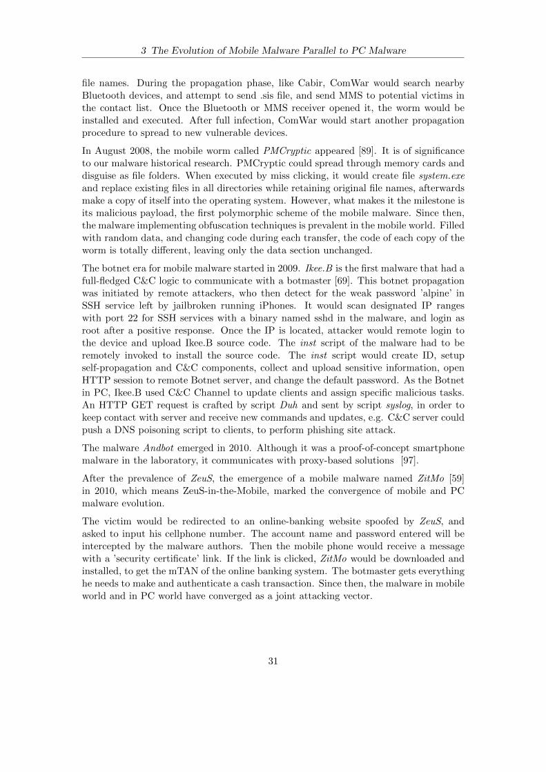
3 The Evolution of Mobile Malware Parallel to PC Malware
file names. During the propagation phase, like Cabir, ComWar would search nearbyBluetooth devices, and attempt to send .sis file, and send MMS to potential victims inthe contact list. Once the Bluetooth or MMS receiver opened it, the worm would beinstalled and executed. After full infection, ComWar would start another propagationprocedure to spread to new vulnerable devices.
In August 2008, the mobile worm called PMCryptic appeared [89]. It is of significanceto our malware historical research. PMCryptic could spread through memory cards anddisguise as file folders. When executed by miss clicking, it would create file system.exeand replace existing files in all directories while retaining original file names, afterwardsmake a copy of itself into the operating system. However, what makes it the milestone isits malicious payload, the first polymorphic scheme of the mobile malware. Since then,the malware implementing obfuscation techniques is prevalent in the mobile world. Filledwith random data, and changing code during each transfer, the code of each copy of theworm is totally different, leaving only the data section unchanged.
The botnet era for mobile malware started in 2009. Ikee.B is the first malware that had afull-fledged C&C logic to communicate with a botmaster [69]. This botnet propagationwas initiated by remote attackers, who then detect for the weak password ’alpine’ inSSH service left by jailbroken running iPhones. It would scan designated IP rangeswith port 22 for SSH services with a binary named sshd in the malware, and login asroot after a positive response. Once the IP is located, attacker would remote login tothe device and upload Ikee.B source code. The inst script of the malware had to beremotely invoked to install the source code. The inst script would create ID, setupself-propagation and C&C components, collect and upload sensitive information, openHTTP session to remote Botnet server, and change the default password. As the Botnetin PC, Ikee.B used C&C Channel to update clients and assign specific malicious tasks.An HTTP GET request is crafted by script Duh and sent by script syslog, in order tokeep contact with server and receive new commands and updates, e.g. C&C server couldpush a DNS poisoning script to clients, to perform phishing site attack.
The malware Andbot emerged in 2010. Although it was a proof-of-concept smartphonemalware in the laboratory, it communicates with proxy-based solutions [97].
After the prevalence of ZeuS, the emergence of a mobile malware named ZitMo [59]in 2010, which means ZeuS-in-the-Mobile, marked the convergence of mobile and PCmalware evolution.
The victim would be redirected to an online-banking website spoofed by ZeuS, andasked to input his cellphone number. The account name and password entered will beintercepted by the malware authors. Then the mobile phone would receive a messagewith a ’security certificate’ link. If the link is clicked, ZitMo would be downloaded andinstalled, to get the mTAN of the online banking system. The botmaster gets everythinghe needs to make and authenticate a cash transaction. Since then, the malware in mobileworld and in PC world have converged as a joint attacking vector.
31

3 The Evolution of Mobile Malware Parallel to PC Malware
3.5 Relating both Timelines
Everything that happened yesterday in the PC world and will happen again in the mobileworld tomorrow, just like a Groundhog Day. In Fig. 3.1 we have connected related eventsin the PC and mobile malware evolution with dotted lines. There is an obvious relationbetween both timelines in every evolution step. They follow the same sequential pattern:from the first worm, proof-of-concept though, to the first successful self-propagationworms showed up in both fields with fully functional exploit components, to the firstbotnet with very complete Command and Control logic, every development step of PCmalware and mobile malware is almost the same.
However, there is one point of divergence related to the emergence of the dialer. Itemerged at the early stage of the mobile malware development in 2004, but at the laterstage of PC malware development in 2001, drawing a relatively close time lapse. This isbecause the it is much more convenient for the attacker to make money from the mobilephone than a PC.
The appearance of ZeuS is a significant point throughout the history of malware. It isthe first time a malware could transcend the PC world and combine it with the mobile.Since then, the development of mobile malware caught up with and started to keep pacewith the PC malware.
From the both of the time lines we can learn that the obfuscation techniques emergedat relative early period of the malware evolution process, and simultaneously at theapproximately same developing stages. After that, those techniques are prevalent amongthe malware in both of the platform.
3.6 Conclusions
The purpose of digging into the dark history is to vision a brighter and clearer future.
After all this research, inevitably we would come to this question: Will the two devel-opments synchronize at a certain point in the near future? Will the previous threats inthe PC world repeat itself in the mobile world?
The answer to the two questions is probably yes. Firstly, the quantity of mobile bankingtransactions is on the rise, and still has very large growth potential. Secondly, accordingto the survey of TREND [62], financial crimes have not yet become a mainstream, buton a way since ZitMo. Thirdly, the increasing computing power of the smartphone blursthe boundary between mobile and PC in our daily life. Sometimes, a smartphone couldbe a more handful tool for some activities, e.g. surfing the Internet, checking Facebook,sending and receiving email, or even online banking. The launch of Ubuntu Phone,which merges those two together, would exacerbate this trend.
Although the ZeuS botnet is already prevalent in the PC, there is no similar malwaredesigned for the mobile. In the future, there could be a mobile botnet targeting bankaccounts, just like ZeuS, but only installed on smartphones.
32
3 The Evolution of Mobile Malware Parallel to PC Malware
--
DesktopTim
eline
MobileTim
eline
t1971Cr
eeper
t1981El
kClon
er
t1984Ba
ckdoor
t1986PC
-Write t
1988M
orris
t1990Ch
ameleon
t1999Pr
ettyP
ark t
2001Di
aler t
2002Sla
pper
t2007Ze
uS
t2004 Ca
bir, D
ust,Mosquit,
Brado
t2005
ComW
ar
t2008 PM
Cryptict
2009
Ikee.B
t2010 An
dbot, Z
itMot? ?
Figure 3.1: Malware Timeline
33

3 The Evolution of Mobile Malware Parallel to PC Malware
It works like a rootkit containing a keylogger hiding in a native library. It automaticallydetects online banking activities, e.g. bank websites, online banking applications, andtries to steal account numbers and passwords, transfers them back to dropzone, andintercepts mTAN.
The purpose of this section is to make a prediction about future threats. Then we havethe chance to stop them before it is too late.
34

Chapter 4
The Obfuscation Framework
As introduced in the previous chapter, we approach practical obfuscation as a processto transform the target APK into a more complex form while not significantly slowingit down. We design a Python based framework not only to automize the obfuscationprocess, but also to carry out performance measurement and optimization simultane-ously. In this chapter, we introduce the components and their working scheme in theframework, and more importantly the Obfuscation Management Layer which controlsevery work flow of the framework.
4.1 Introduction
The framework is designed to iteratively select and apply different obfuscation methodsto the input APK programs, and then evaluate the complexity and similarity of the resultAPK programs. To implement different obfuscation strategies, it can integrate differentalgorithms into the Obfuscation Management Layer to guide the transformation process,and to compare the distinguished results. The algorithm will be introduced in theChapter 6. The framework can be freely extended by adding new obfuscation methods,new software complexity metrics, and new algorithms, as we do in the following chapter.
The framework contains the following modules: the obfuscation engine Pandora [74], thecomplexity metric evaluator SSM, the similarity measurement toolset Androguard [34],the dynamic performance analysis tool Profiler [5], the GUI input generating and testingtool, the Android hardware device, the Preprocess and the Postprocess toolset, and thefile system with the database.
The structure of the framework is depicted in Figure 4.1. To make the work flows ofthe framework easier to understand, we distinguish the connections between modulesas data flows and control flows. In this Figure, the blue arrows represent data flows,e.g. the fetched APK files stored in the File System, the transfer of the log files fromthe Testing Tool to Profiler etc.. The black arrows represent control flows, such as theinquiry command from the Obfuscation Management Layer to the Database, or the copypaste command to the File System. Because the Obfuscation Management Layer, thePandora, and the SSM cooperate more closely with each other than other modules, weintegrate them as one central module in this figure. The Androguard is also integratedinto this module. However, since the measured similarity values from the Androguardare only used as an index of the differences of the transformation results, and do notaffect the obfuscation process, it is not explicitly represented in the figure. Its relatedworking process will be introduced in Section 4.9.1.
35

4 The Obfuscation Framework
Dat
abas
e Fi
le
Syst
em
Pre
pro
cess
Post
pro
cess
An
dro
id
Pro
file
r
Test
ing
Too
l
Dev
ice
Ob
fusc
atio
n M
anag
eme
nt
Laye
r Pan
do
ra
SSM
Dat
a Fl
ow
Co
ntr
ol F
low
Log
Fig
ure
4.1:
Th
eF
ram
ewor
k.
36

4 The Obfuscation Framework
Now the working iteration of the framework will be briefly introduced.
In the beginning, the Obfuscation Management Layer (OML) will fetch target APK filesaccording to the database information, and then push it into the Preprocess module. ThePreprocess will unzip the APK into the Jar file and input it into the central module.At the same time, the APK is also input into the Testing Tool module to generate thetesting cases log, if the APK’s log file does not exist. The obfuscation starts when thecentral module receives the Jar file. According to the Database history, the OML selectsa suitable obfuscation method and the obfuscation engine Pandora applies this methodto this input Jar file. The SSM module measures the complexity metrics of the result Jarfile, compares values before and after obfuscation. All the data are then recorded intothe Database. The OML will judge if the result has reached our desired complexity, anddecide whether next iteration should proceed. After that the result Jar file is transformedto Dex format and zipped into the APK by Postprocess module. The Profiler moduleimplements performance test with the testing cases log for the two APKs to comparethe performance penalty caused by obfuscation. The results are returned to the OML.All the files, logs, and data are stored into the File System and the Database.
4.2 Pandora
To make reverse engineering for Android application more difficult, Protsenko etl. [74]developed the Android obfuscation framework — Pandora (PANDORA: Applies Non-Deterministic Obfuscation Randomly to Android). It is a Soot [92, 93] based trans-formation system which operates on Android bytecode level, and aims at importingrandomness as a factor to make transformation results as non-deterministic as possible.
Soot framework [92] includes four intermediate representations, the stack based low-levelBaf, its Static Single Assignment form Shimple, the register based medium-level Jimple, and with its the aggregated version—Grimp. To transform the Dalvik bytecode, Pan-dora uses the Jimple representation. Because its strong typing and its limitation to 15different 3-address based instructions, it is more convenient to analyze, optimize, andproduce the result bytecode than theDalvik bytecode which has untyped 218 instruc-tions. The transformation of Pandora is implemented by the two extension modules ofthe Soot framework, the BodyTransformer and the SceneTransformer during its compileprocess. In this process, all the Object-Oriented elements are represented by the 15 Jim-ple instructions, and transformed locally and globally with the Jimple TransformationPack (jtp) and Whole-Jimple Transformation Pack (wjtp).
For the sake of simplicity, we call “obfuscation transformation” as “transformtion” inthis thesis.
In the following part, we demonstrate the theories and the implementations of thesetransformation methods that constitute the BodyTransformer and the SceneTransformerextension modules. Pandora has 11 obfuscation methods, including 6 data and con-trol flows obfuscation (the Java method level obfuscation), 5 Object-Oriented obfusca-tions(the Java class level obfuscation), and an identifier renaming obfuscation. It can
37

4 The Obfuscation Framework
apply an arbitrary subset of these obfuscation methods to the Android applications. Be-cause the identifier renaming has no effect on the complexity metric, and its relation tothe “difficulty” level against human revere engineering has already been elaborated in thework of Ceccato etl. [24, 25, 23], we emphasize the first two categories of transformations.
4.2.1 Data and Control Flow Transformation
This type of transformations is developed to obscure local and global variables, andtherefore the operations on the basic data types and objects.
String Encryption This transformation provides two kinds of polyalphabetic stringencryption algorithms, which replace each string with a serial of different characters. Adiversity of substitution methods is provided to obscure the strings which are revealingkey information, e.g. “Login Failed”. This transformation method is flexible to inte-grate more encryption algorithms to enhance diversity. The decryption algorithms areadditionally embedded into the source code of the target application. More effort forthe reverse engineer is needed to revert embedded algorithms to the original strings.
Vigenere Encryption: This algorithm improves Caesar Cypher [87]. It encrypts thetarget strings by determining the symbols in the strings with periodical shifting. Ituses another string as the key for decryption.
Dynamic Key Encryption: This algorithm is the upgrade of Vigenere Encryption.The shifting is defined by a series of randomly generated key ki by the Linear Con-gruential Method [55], with the given initial key k0.
Integer Encoding Besides the unencrypted Strings within the Java program, the inte-gers in this program can also imply critical information that can assist reverse engineer-ing. Therefore Pandora provides two algorithms, Split Modulo and Linear Encoding, toobscure the integers by adding extra homomorphic operations. In this way the decodingto the original values on the run is not necessary, so that the performance loss can besaved. The details of the two algorithms for the homomorphic encoding are describedas follow:
Split Modulo
With any given integer, the x P I can be decomposed into the quotient and the remainder.With natural number m, exist a and b and that the following equations are accepted:
a xm, b x mod m
where the “/” denotes the integer division.
38

4 The Obfuscation Framework
Then any two integer numbers x1, x2 P I can do the operations of addition, subtraction,multiplication, and comparison without using their original values [58]. We take additionfor example. m values are randomly and locally (within this Java method) identical, thequotient and the remainder of x1, x2 are respectively pa1, b1q and pa2, b2q their additionresult is:
a a1 a2 pb1 b2qm, b pb1 b2qmod m
Then the addition result of x1, x2 can be restored dynamically only when necessary.Therefore all the integer and their calculations are protected through out the wholecomputing process.
Linear Encoding
The same as Split Modulo, Linear Encoding encodes the integer variables in the wholedata flow, and decodes dynamically in JVM/Dalvik/Art. However, instead of encodinginto the quotient and the remainder, it encodes the target variables x into z with lineartransformation as the equation:
z αx β, α, β P N
where the Natural Number α, β are randomly assigned. Thus the transformed integervariables can be computed without decoding and the therefor protected.
Array Index Shift Array is an important data structure in Java. This transformationmaps all the elements in the array to a different sequence. It makes their index lookstotally random, therefore obscuring the loop of the array. The application of this trans-formation is only confined to local arrays. Because if the whole array passes to anotherJava method as one parameter, the effect of obfuscation is limited.
Locals Composition This transformation composes the local variables, e.g. integers,chars, or strings, into containing objects. It is used to obscure the correlation amongthose independent and unrelated values, so that they appear to be semantically closelyrelated. To compose the locals, a set of same type variables are chosen and compressedinto the equal type of map or array, i.e. local integers to integer array, local strings tostring array (or map). All those compressed variables are accessed by the indexes of themap or the array.
Compose to Array : The length of the array will be r0, n 1s, n is the number ofcompressed elements (local variables). The index n 1 stores the number “n”. Theindex of each element is randomly assigned.
Compose to Map: The same type of the local variables and their generated indexeswill be stored into one java.util.HashMap object. The type of the indexes (the key ofthe hash), which includes the integer, the char, or the string, is randomly selected.For each of the HashMap, only one type of the key is used.
39

4 The Obfuscation Framework
4.2.2 Object-Oriented Design Transformation
The following obfuscation methods, which composite the other half of the Pandora sys-tem, are constituted by the SceneTransformer extension modules. The goal of theObject-Oriented Design obfuscation is to move, modify, replace, and integrate the ele-ments within the Java objects, such as fields, methods, and classes, so that the appear-ance of those objects will be changed.
Drop Modifiers Drop modifier is an essential transformation for the total obfuscationprocess. It alters the access restriction for the classes and all their elements by replacingall the modifiers of the fields, methods, classes with public and removing final. All theother OOD obfuscation methods which modify the structures of the objects thereforecan be applicable.
Extract Method Extract Method refactors the Java methods by outlining the wholebody of the given methods. It generates a new Java method with the same argumentsand the same method body, while replacing the whole body of the given method with astatement to invoke the new method and pass the arguments.
Extract Method is not only a obfuscation method, but also a preliminary preparationfor further transformation. It is because in Java or Android, the signature of a setof particular method cannot be changed, e.g. the Java entry point main method, theAndroid onClick methods and the onCreate methods in the MainActivity class. Toapply OOD obfuscation on those methods (with Merge Methods for example), methodbody outlining is necessary.
Encapsulate Fields Encapsulate Field creates a getter method to define the valueof the target field and uses a getter method to extract this field. Therefore the targetfield can be encapsulated to avoid direct access, and allow modification and furtherobfuscation on that transformed field, i.e. the getter method. Consequently, EncapsulateField will change software complexity of the structure and the appearance of the callgraph in the target Object, and thus confuse similarity algorithms.
Move Fields Move Fields transfer the fields from one class to another. For the staticfield, the references to this field need to be updated. While for the instance field, sincethe base object (moved-out class) instance for this field is required, the moved-in classmust create a new reference corresponding to the moved-out class, to initialize it beforethe moved field is used. Furthermore, the based object instance will be constructed onlyonce and remain unchanged afterwords, until the life cycle of the moved-out class isfinished.
40

4 The Obfuscation Framework
Move Methods Similar to the Move Fields, the static methods are replaced by theinvoking statements while the instance methods need the base objects. However, thesynchronous life cycles of the moved-in and moved-out class instances are not necessary,because the reference to the moved-in class is available for the call sites.
As introduced before, some of the Java methods, e.g. onClick, onCreate which are calledfrom outside of the program, or overloading of the abstract methods from interface orsuperclass, are not applicable for Move Methods.
Merge Methods The Merge Methods is to combine two methods in the same classwhich have the identical return types and modifiers. After merging, the bodies of twoprevious methods can be interleaved in the newly merged method, while the executionof different bodies are chosen by the if...else... condition. The parameters lists of theprevious methods are attached together as one input list of the new method, along withthe extra bool variable which controls the if condition.
4.3 Androsim
In order to spot and scale the identical, similar, and distinct methods between twoAndroid dex files and thus the over all difference ratio, we select Androsim as ourmeasurement tool. This tool is described in the publication authored by Desnos etl.[70], as built for measuring and evaluating the distance of bytecode similarity betweentwo APKs to prevent plagiarism.
Androsim consists of similarity comparison algorithm Normalized Compression Distance(NCD) [27], that computes the distance between two series of strings which are com-pressed by snappy [3], and a module to translate the raw binary of dex file into arepresentation signature string, which is the input of that NCD algorithm.
In order to measure bytecode similarity between two dex files, the method signaturesfrom each of the Dex file are generated by that translation module. This signature isa concise form of representation for the raw binary file, and is created based on SilvioCesare grammar [26]. To generate this signature, the identical methods between the twodex are firstly excluded by comparing the checksum of the instruction sequence amongall those methods. Secondly, the features of control flow graph, i.e. BasicBlock, If,Goto, Return etc., along with the API, and the Exceptions are represented sequentiallyby chars which are mapped from the dictionary of Silvio Cesare grammar [26]. Thosegenerated char serials (strings) are the input of the following NCD algorithm.
The Normalized Compression Distance is defined as dNCDpA,Bq. A,B are two in-put strings. With the compressor C (snappy), the length of the compressed string areLpCpAqq and LpCpBqq (abbreviate as LA and LB). A|B are the concatenation (jointogether and get rid of A’s common string) of A and B:
41

4 The Obfuscation Framework
dNCDpA,Bq LA|B minpLA, LBq
maxpLA, LBq
With this equation, the similarity of two methods can be computed. Thus the overallsimilarity of the two dex file.
4.4 SSM
For software vendors, quality of their products plays a key role for their market status.However, quality is not an index that can be directly assessed and intuitively exemplified,and it is hard to control during the development process. To improve and control thequality of program design and development, the software complexity metrics are used tomodel and quantify the quality. [53][103]
The software complexity metrics are not only used during software (re)engineering tomeasure and evaluate the quality of the programs, also they could indicate produc-tivity [53], estimate and project reliability [54], improve maintainability [52], predictperformance [32], and meanwhile reflect the difficulty of understanding the program.
In our research, we integrate SSM into our framework to measure the different softwarecomplexity metrics, for the static analysis of the obfuscation results.
With the input Jar file, the SSM works as follows: To measure the metrics, the SSMfirstly profiles the relation of the classes and methods in the target Jar file with a set ofObject-Oriented Design metrics, and then identifies the data or control flow within eachJava method. Meanwhile, it generates the analysis graphs, e.g. the class inheritancediagram, the method call graphs, the control flow graphs etc.. After that it evaluatesthose output graphs and generates the results data. These data are later used to eval-uate and characterize the obfuscation methods and then joined with the performancemeasurement to optimize the obfuscation results.
Same with Pandora, the SSM module is also developed based on the Soot framework,using Jimple as the intermediate representation (IR). SSM evaluates software complexitymetrics in both the Object-Oriented Design aspect (Java class level) and the Controland Data Flow aspect (Java method level).
4.4.1 Method Level Metrics
Cyclomatic Complexity Control Flow Graph (CFG) is the abstract form of operationlogic that represents the specific module (method) in software with an explicit entrynode (call) and exit node (return). Each possible way of execution in this softwaremodule corresponds to a traverse path from entry node to exit node in the CFG. Thedifferent way of execution depends on the values of the predicates in condition switchstatements like if, while, etc.. To fully test or understand this module in the software,
42

4 The Obfuscation Framework
all the possible paths in this CFG need to be covered by giving different bool values tothe predicates. Therefore, if there exist more possible execution paths in the CFG, itrequires more efforts to totally test or understand this software module. Thus it wouldbe more complex for reverse engineering.
To quantify this complexity, the total number of possible paths need to be calculated.In Graphs Theory, the CFG could be recognized as a strongly connected graph witha virtual directed edge added which points from exit node to entry node. The totalpossible paths of this modified CFG, which are recognized as the fundamental cycles inthe Graphs Theory, are computed as pe 1q n 1.
So, this Cyclomatic number formula, by simply adding one virtual edge, defines themetric Cyclomatic Complexity [95].
Dependency Degree DepDegree is the number of the directed edges in the depen-dency graph that models the data dependency relation among the operations (nativeinstructions) in the method [17]. Therefore the dependency graph is the data-flow graphin the operations level. It is consisted of the nodes which represent every native codeinstruction in the method, and the directed edges which represent data flows or depen-dency relation between those nodes (instructions). The dependency relation means that,in data flow graph, the variable in node A is defined by the assignment or function calloperations in node B. Thus, there is a directed edge pointing from node A to B.
For the whole program, DepDegree is the index of how much information has to bedealt with and how many different data states have to be processed during reverseengineering. For every single node, it represents the amount of the predecessor operationsthat need to be considered, which decide the current state of operation node. If thereare more possible states for each node in the data-flow graph, it would be more complexto comprehend or optimize the program [17].
Lines of Codes The Lines of Code (abbreviated as LOC) is a simple widely-usedmetric for measuring the quantity of lines of text in the source code and the size of theprogram [98].
LOC was traditionally associated with programming errors in the predictive models.Early research [12] shows that bug density of the Fortran modules, which has less than200 LOCs, is inversely correlated with the quantity of LOC. Another research done inthe same period [82] also shows that, when the LOC is above 500, the bigger moduleshave a higher bug density regarding to Pascal, PLS and assemble language.
However, the LOC metric cannot indicate the real complexity of each code line [98].Meanwhile, it loses the information of overall structure complexity of the programs (e.g.branches, loops). Therefore, LOC metric is usually combined with other metrics toprovide more comprehensive measurements to the programs.
43

4 The Obfuscation Framework
4.4.2 Class Level Metrics
Weighted Methods per Class (WMC): the number of the methods defined in a class.
Depth of Inheritance Tree (DIT): the number of classes along the path from the givenclass to the root in the inheritance tree.
Number of Children (NOC): the number of direct subclasses.
Coupling Between the Object classes (CBO): the number of coupled classes. Here,two classes are considered coupled, if one of them uses methods or instance variablesof the other one.
Response Set for a Class (RFC): the number of declared methods plus the numberof methods the declared ones call.
Lack of Cohesion in Methods (LCOM): Given a class C declaring methodsM1,M2, ...,Mn
and a set of instance variables used by the method Mj denoted as Ij , define P tpIi, Ijq|Ii
Ij Hu and Q tpIi, Ijq|Ii
Ij Hu. Then LCOM maxt|P |
|Q|, 0u. Intuitively, if the cohesiveness is low, the original class should be split intotwo or more classes.
4.5 Preprocess Module
For the preparation of the optimized obfuscation, the Preprocess module is used to fetchand process different files or data from the File System according to the requirementof the Obfuscation Management Layer. Before the obfuscation starts, firstly a newAPK from File System is input into this module. It then unzips the new APK toextract the Dex file, and translates into the Jar file with the tool dex2jar [2]. If thisAPK has been transformed before, the Jar file will already exist. According to therecords in the Database, the Jar file will be fetched directly from the File System.Those unzipping and translation steps will be bypassed. Finally, the Jar and the APKare all sent to the central module (includes the Pandora, the SSM, the ObfucationManagement Layer, and the Androsim) to continue the transformation process. Whenthe performance optimization parts are integrated in the framework, the Preprocessmodule will meanwhile start the Testing Tool module. It will then forward the APKinto this module, wait for the result logs, and store it back to the File System which willbe fetched at the disposal of the Obfuscation Management Layer.
4.6 Postprocess Module
When the obfuscation transformation is finished, the Jar files, the SSM and Profilerlog files are input into this module. For the Jar file, it firstly will be optimized bythe Jasmin [61], then translated into the Dex file, and finally zipped into APK. ThisAPK file will be sent back to the Obfuscation Management Layer for comparing of the
44

4 The Obfuscation Framework
APKs’ similarity before and after obfuscation by Androsim. For the SSM log files, it willcompute the sum up values of complexity metrics of this Jar. The complexity resultsare also sent back to OML to measure the differences. For the Android Profiler log files,it calculates the total CPU cycles of those applications from the logs. After that, theAPK, the Jar files and the log files are stored into the File System, and all of the resultsdata from the computations are updated into the database.
4.7 Automatic Black Box Testing
To improve the code coverage in this performance analysis, we develop a black box testingtool which can be widely adapted to all Android applications, automatically generatingGUI behaviors on the run, and exploring as many APK functions as possible.
During the development process of this Android black box testing tool, there still existseveral problems we need to pay attention to. Firstly, our testing tool is trying to usethe greedy searching method to invoke all the functions in the APKs, which can causeinfinite loops in the tests. For instance, button A in Android view M lead to viewN , yet button B in view N vice versa. Secondly, the re-invoking of the functions willredundantly execute particular sections of codes. That can cause the recalculation ofthe CPU cycles during performance profiling.
To solve these problems, the view in the activity needs to be identified and a suitabletraversing algorithm for the GUI tree has to be implemented. We use the view hashvalues to recognize every Android GUI view. And then we record the view status changeswhen our tool clicks each of the clickable UI elements (e.g. buttons, slides bars, and etc.),i.e., we can record in the log files which view this button belongs to and what is the nextview when this button is clicked. We implement “Deep-Priority Search with One StepBack” algorithm in the testing tool, which can avoid view looping with the help of thehash values. When all the clickable UI elements have been traversed, the algorithm willterminate the testing.
4.7.1 The Implemented Tools
Because our black box testing tool can only acquire information of current view onthe screen during runtime, the context of predecessor and successor views have to beestablished from the log file as the program runs, i.e. we record the changes of the viewsin the log file when a button is clicked, and then a directive traversing graph of thecurrent APK GUI is constructed.
The “Deep-Priority Search with One Step Back” algorithm is iteratively launched todetermine the strategy of selecting the next GUI element to construct this graph. Ineach of the iteration, firstly the connection is established from the host machine (theTesting Tool module to be exactly) to the Android testing device. Then the data streamof the current view on the screen is received by the Testing Tool module in the host
45

4 The Obfuscation Framework
machine and interpreted into the tree data structure. With the help of the tree datastructure and the traversing history log file, the algorithm is applied to select and invokethe next element to traverse, and record into the log.
In the above procedures, the connection, the data stream interpretation, and the invokingof the active or clickable elements are crucial. We implement the following tools for thosefunctions.
1) view server : A service running on the Android device. Android GUI the view isinherently a tree data structure that formulates the screen layout on Android devices.The view server dynamically acquires the data of the current view each time it updates,and transforms them into the data stream. It is connected by the socket or the telnetfrom a local host machine running the debugging software (solointerface in our case). Ittransfers the stream data of view that end with “Dump -1”. After that the data transferis suspended until a new view layout shows on the screen.
2) solointerface: Our testing tool uses Apk View Tracer tool [4] to connect to the serverin android devices. When the APK is running, it retrieves information about the viewin the current screen. All the elements in that view and with their details (e.g. name, id,clickable or not, position etc.), are edited into an node object sets, and then compressedinto the tree data structure. The connection is established by telnet or socket. Whenthe view is changed, the view list will also be updated. The nodes will be processed bythe Tracer module listed in the following section, to produce a directive graph.
3) ViewTracer : This module is the GUI input generator in our testing tool. It processesand records all the information passed by the solointerface, features and recognizes thecurrent view or keys waiting to be clicked, and then call the monkeyrunner to make aclick or other action on the device screen.
4.7.2 The Algorithm in the Testing Tool
Before starting the algorithm, we need to create 3 data structures, for the storage ofinformation during runtime.
1. UI elements: To identify the views, we construct the data structure UI elements.Firstly, it hashes all the UI elements in each view with their id, coordinates and class-name. And then, we used the hash numbers of the views as index paired with a list,which is composed by all of the clickable UI elements within that view. Each UI ele-ment contains the following information: [id, text, isClicked, coordinates, classname,locations]. The Boolean flag “isClicked” is the variable that records the traversingstatus of each UI element. If traversed, the “isClicked” is valued True, otherwiseFalse.
2. UI hash list : It contains the hash values of each different UI interface which hasappeared on the screen of the Android device. It is the list of index from UI elements
46

4 The Obfuscation Framework
3. key list : It sequentially records the clicked UI elements (buttons) which will be outputto the result log file. It contains information of each key’s location, text, button id,the affiliation UI, the next UI after click. During the performance profiling process,the APK would have the same UI elements invoking order with this key list.
1
2 Terminate = True
3
4 While(Terminate)
5
6 Extractor(current UI elements data) from view server
7
8 update key_list of the next UI
9
10 if current UI is new
11
12 UI_hash_list.attach(hash of current UI)
13
14 UI_elements.attach(pair of hash and objects list)
15
16 if current UI is not fully traversed
17
18 for elements in current UI
19
20 if element is clickable and not clicked:
21
22 generate click event
23
24 update in the elements list
25
26 break for
27
28 continue While
29
30 else:
31
32 if any key leads to the other not fully traversed
UI:
33
34 click this key
35
36 update key_list
37
38 continue while
39
40 else:
41
42 press back button
43
47

4 The Obfuscation Framework
44 update key_list
45
46 if all UI have been traversed:
47
48 Terminate = False
Listing 4.1: Overall Algorithm of Black Box Testing Tool
The algorithm is shown in the List 4.1. Before the main while loop begins in thealgorithm, the loop breaking condition Terminate is valued as True, to keep the loopsrunning until the termination condition is satisfied, which is when all the clickable UIelements in all the views are traversed.
After the while loop begins, firstly the function Extractor() receives the stream datafrom the view service which can provide information of the current GUI on the testingAndroid device.
Unclickable or invisible elements are filtered out from the stream data, which will berestored into the tree data structure (in solointerface). The tree nodes are the clickableUI element objects and also contain all the necessary information of those UI element.
To identify the view, we hash the useful information (e.g. the ID, the coordinates, theclassname) of all the tree nodes as an index. If this view is new, the index hash valuewill be attached to the UI hash list. The pair of hash value and tree nodes (the clickableelements in a view) list is attached to the UI elements. Those objects in the list alltagged the “isClicked” with False as introduced above.
After that, the algorithm starts to search for the traversing route. Firstly, it checkswhether all of the tree nodes (the clickable elements) in this view are clicked. If not,it starts the for loop to iterate on those elements to find the unclicked element. ThenGUI input action is generated from the ViewTracer to click on the element. Then theUI elements is updated by valuing the “isClicked” of the selected element as True. Alsothe key list (the result log file) is updated by adding this new element information tothe list end, which is location, text, button id, the current view and the new view.
Because after the element is clicked, a new view may emerge on the screen. If so, thenew iteration of algorithm has to be started. Thus the while loop executes continueafter the click. And the new view in key list will be updated at the beginning of thenew while loop.
In the case of a fully traversed view, the algorithm will search in the key list, to findall the particular elements in the key list which direct to a different view. In the otherview, the algorithm tries to find out if there still exist elements not traversed yet, bycross referencing the information of “isClicked” in the UI elements list. If they exist,one particular element in the current view will be clicked to go to the new view. Andthen the algorithm replicates the procedure of updating the key list, and continues onthe while loop.
If the current view has been fully traversed and the other view which directly connects
48
4 The Obfuscation Framework
to this view is also totally traversed, the back button is clicked. After updating thekey list, the algorithm will search whether all the elements have been traversed in thisAPK from the UI elements. If true, the loop condition Terminate will be valued Falseto end the while loop.
Extract() module is composed by solointerface() and uiProcess() methods. The soloin-terface() uses telnet to connect to the service view server in Android devices. Eachconnection will return view stream data. solointerface() processes the data and revertthem into the view tree in local host. And then the uiProcess() is used to iterate thosetree nodes.
4.8 Android Profiler and Device
We implement the Android Profiler to measure the CPU time with which the target APKhas to spend on the dynamic testing of the script from the Testing Tool. It composed bythe ViewTracer and the native profiling module of Android OS. The ViewTracer modulehas already introduced in the Section 4.7. The natice profiling module will be invokedby the adb command line and run as a single profiling thread after the initialization ofthe APK process. The command line to initiate the process of the target APK and theprofiling thread is listed as follow.
1 adb shell am start -n <COMPONENT > --start -profiler <FILE >
The n COMPONENT ¡ specifies the activity component of the target APK withpackage name prefix to invoke an explicit intent, such as the com.caynax.alarmclock/.Mainactivity,and the FILE ¡ is the location where profiling log file stores. When this commandis received by the adb daemon in the Android OS, the arguments am start ... will bepassed to the ActivityManagerService daemon, which we have already introduced in Sec-tion 2.2.1. The process of the target APK is created by forking the zygote process whenthe start n COMPONENT ¡ message is received by the ActivityManagerServiceand communicate to the zygote socket as described in Section 2.2.2, while the profilingthread is already initialized in the ART vm by the –start-profiler (Subsection 2.2.2).Therefore the APK process starts along with the CPU time is already recording.
We employ the Samsung Galaxy S II (i9100) which implements the customized AndroidOS Cyanogen OS 5.0 as the Device module.
4.9 Work flows of the Framework
After the introduction of modules, we now explain the work flows of the framework. Wehave three types of obfuscations work flows. Firstly, a number of APKs are obfuscatedwith the same transformation methods multiple times and then the attributes of thoseobfuscation methods, which are measured by the complexity metrics, are observed. This
49
4 The Obfuscation Framework
is the base of our further research on the complexity or performance optimization. Thispart requires a simplified version of the framework without Obfuscation ManagementLayer (OML), and will be introduced in Chapter 5.
Secondly, certain algorithms in OML select the suitable transformation methods to guidethe obfuscation process, to optimize the target APKs into the desired result complexitymetrics. The algorithms will be introduced and compared in Chapter 6. In this part allthe dynamic analysis modules, e.g. the Testing Tool, are not initialized.
Thirdly, while the target APKs are obfuscated to the desired complexity metrics, theperformance of the result APKs are also optimized by the algorithm, to minimize theperformance penalty imposed by obfuscations. The details of the profiling process willbe introduced in the Chapter 6. All the modules are functional in this part.
4.9.1 Software Complexity Optimizations
The overall obfuscation process of the our framework is depicted in Figure 4.2. Thissection is the second type of work flows in the framework. As shown in this graph, each ofthe block colored black represents a functional module as introduced. The central modulecontrolled by OML dominates the whole optimized obfuscation process. It initializesall the framework modules when receiving the obfuscation starting command and thedesignated complexity metric values. We will elaborate one iteration of the workingprocess of OML independently, and the other accessory modules in the framework as awhole entirety will be introduced in the following subsections.
Obfuscation Management Layer (OML) The combination of the Pandora, SSM,and the Obfuscation Management Layer is called the central module of the framework.Because the control and data flow exchanges among those three modules are more regularand synchronous, the three modules could basically be recognized as one integratedentirety for the predigest of our framework work flows. This integrated module worksas follows:
Firstly, when the designated complexity metric values assigned by the user and theprevious iteration obfuscation are received, OML accepts the Jar file from the Preprocessmodule. After that, it starts the SSM module to measure a set of the complexity metricsof this Jar file. Meanwhile, OML sends a series of requests to the Database module. Itthen evaluates if the satisfaction of the target metrics should be expected in this iterationby any transformation method from Pandora.
We have two kinds of searching algorithms available to evaluate the result data returningfrom the Database in this case. Those two search algorithms, which will be thoroughlyelaborated in Section 6.4, are based on either the mean values (the simple search) orstatistics and probability models (the Naıve Bayesian Classifier).
On one hand, for the mean values based algorithm, OML will choose the transformation
50

4 The Obfuscation Framework
Dat
aBas
e
File
Sy
stem
Pre
Pro
cess
Post
Pro
cess
An
dro
id
Pro
file
r
Test
ing
Too
l
De
vice
Ob
fusc
atio
n M
anag
eme
nt
Laye
r Pan
do
ra
SSM
Dat
a Fl
ow
Co
ntr
ol F
low
1
2
3
3
4
4
5
6
7
8
9
Fig
ure
4.2:
Th
eF
ram
ewor
kof
Ob
fusc
atio
nw
ith
met
ric
op
tim
izati
on.
51

4 The Obfuscation Framework
Obfuscation Management Layer
SSM Pandora
An
dro
sim
Figure 4.3: The Obfuscation Control Module.
method whose average metrics increase are the closest to the target values (in Euclideandistance).
On the other hand, for the statistics and probability models, OML will calculate theoverall probability of reaching the target values, no matter what method it chooses. Thedetails are shown in Section 6.4.3.
If this probability is low, OML will search the Database to calculate the metrics valueswhich could possibly be reached at this obfuscation iteration. And then it substitutesthe target metrics with the possible values. If the possibility is high, OML starts tocalculate all the probability of the transformation methods for the target values, andthen select the dominant method.
When the transformation method is determined, OML will forward the Jar file to thePandora along with this method as an argument. Then the obfuscation process is started.The SSM module is used again directly after the transformation is applied. With thehelp of Postprocess module, the result metrics values are processed and compared tothose before transformation (after Step 7 in Figure 4.2 by SSM).
Afterwards, OML starts to examine the results, to measure if the temporary metrics orthe target metrics result are reached.
If the target metrics are satisfied, the total transformation process will be terminatedafter this iteration. If only the temporary values are reached, our framework will set
52

4 The Obfuscation Framework
another iteration. That obfuscation result Jar file will be sent to Postprocess module foroptimization, translated into Dex file, and then zipped into the APK afterwords. Theprocedures will be introduced in the next Section 4.9.1.
The new APK file is pushed back into OML to calculate the similarity ratio with theunobfuscated version of the APK file in the Androsim module. The Androsim in thiscentral module is used to measure the APK file before and after the obfuscation, toobserve if any differences have been made to the source codes during this transformationiteration. The Normalized Compression Distance algorithm used by Androsim is not aunique and accurate measurement of the differences between two strings, as introducedin Section 4.3. The result depends on the compression methods implemented. Thus, weonly use Androsim result here as a reference, to check the amount of Java methods inthe Dex file that have been modified or remain the same. The result data of Androsimis still writing into the obfuscated apks table in the Database module.
Workflow of the Framework In this Figure 4.2, the rectangles colored gray meanthe modules which are not functional in this complexity optimization section. The bluearrows are the routes to pass the data, e.g. required database items, APKs, Jars, log filesetc., while the black arrows mean control flow which contain instructions to commandand coordinate the other modules perform particular tasks.
To initialize the framework, the target complexity metric values, e.g. DepDegree and theCyclomatic Complexity, which are set to increase 30% and 50% respectively (Dep0.30^Cyc0.50), are assigned to the target set of APKs and input into the command lineinterface of our framework.
When this initial instruction is received, the central module, which is under the controlof OML, interprets this command as database inquire messages and then sends them tothe Database module (Step 1 in Figure 4.2). The Database module searches in its tablefor the information of the APK in the target APKs set, i.e. name, stored directory etc..
According to this information, instructions are passed from OML to the File System(Step 2) to search for the input APK and data for the Preprocess module. In the followingsteps, our framework will start to transform this APK to the desired complexity metricvalues. When the above searching is finished, all the information, e.g. the previous SSMlog files, is returned to OML (Step 3) for further support of transformation.
From the information, the framework would know if this APK had been transformedbefore. If so, the Jar file of the target APK is already stored in the File System andthe metrics are measured. Then the Jar file will skip the Preprocess module, directlygo to OML, and skip the SSM module before transformation as well. If not, the APKis pushed to Preprocess module (Step 4). In this module, the Dex file is extracted fromthe APK and translated into the Jar file. In this section, performance analysis is notinvolved. Thus, the Testing Tool module (colored gray) will only be initialized by thisPreprocess module in the following section.
When the Jar and the APK are both input into OML (Step 5), the obfuscation process
53

4 The Obfuscation Framework
inside the central module starts as elaborated in Section 4.9.1. During this process,OML will select the dominant obfuscation method , start transforming, and then com-pare the complexity metric values. If the transformation fails, OML will select anothertransformation method and replicate the above process.
To be able to process the transformed Jar file and the data logs from OML, the Post-process module is then implemented (Step 6). It does not only optimize the Jar filewith Jasmin [61], transforms to Dex, and zips into APK (when received from Step 7),it also extracts and processes the log files generated by the SSM module or the AndroidProfiler module implemented in Section 4.9.2 (colored gray).
To measure the NCD similarity ratio made by obfuscation (as introduced in Section 4.3),the Postprocess module will send the obfuscated APK back to central module for theAndrosim comparison. The similarity data are only used in Chapter 5, to show differentproperties of the transformations.
For the received SSM logs(Step 7), it does not only calculate the total values of everymetric in the target Jar file, it also calculates the metrics values for each class.
To evaluate the transformation result, the total metrics values are sent back to OML(Step 7), and meanwhile database is updated (Step 8). This updating process includes:The result information of the APK is stored into the obfuscated apks table, which con-tains the directory, transformation method, its original version, with its similarity andall the other data from the Androsim; The complexity metric information of the APKis stored into the method metrics and the class metrics tables.
The transformed Jar file, the APK file, and the log files are then stored into its directory(Step 9) in the File System.
The above procedures are one iteration of the total obfuscation transformation processof an APK. The iteration continues until the target complexity metrics are satisfied inthis APK. Afterwards, our framework moves to the next target in the APKs set.
4.9.2 Performance Optimization
In the context of software protection, we study how to automatically and practicallyobfuscate a given APK to a given target level of “difficulty” while not substantially“slowing down” the program. To be able to quantify the “difficulty”, we measure itwith the software complexity metrics in our research, and implement our obfuscationframework with the two optimization algorithms to reach the given target level. Theworking process is introduced in previous section.
According to Section 2.3.1, simply optimizing the software complexity metrics is notsufficient for such obfuscation. Performance penalty also needs to be defined, evaluated,and then optimized together with the other complexity metrics. In the following section,we introduce the working process of our performance evaluation and optimization.
54

4 The Obfuscation Framework
Dat
abas
e
File
Sy
stem
Pre
pro
cess
Post
pro
cess
An
dro
id
Pro
file
r
Test
ing
Too
l
De
vice
Ob
fusc
atio
n M
anag
eme
nt
Laye
r Pan
do
ra
SSM
Dat
a Fl
ow
Co
ntr
ol F
low
4.1
4.2
4.4
4
.3
4.5
4.6
4.8
4.7
4.9
4
.9
Fig
ure
4.4:
Imp
lem
enti
ng
the
An
dro
idU
IT
esti
ng
Tool
.
55

4 The Obfuscation Framework
Implementing the Android UI Testing Tool To evaluate the performance, theAndroid Profiler module initiates and launches the MainActivity of the target APK inthe main thread of a ART virtual machine, and uses the profiling threads to log the CPUcycles of every Java method pushed on to or popped from the threads stacks. Launchingthe MainActivity alone however only covers a limited part of APKs’ codes.
To have maximum code coverage, the Testing Tool module is implemented. Figure 4.4shows the work flow of the Testing Tool module in the framework: When the Preprocessmodule receives the information of the target APK (Step 4) , hereafter called “newAPK”, the Testing Tool module will be started (Step 4.1) immediately after.
After receiving the new APK (Step 4.2), the Testing Tool module tries to install thenew APK through the Android Profiler module (Step 4.4). In the process of Androidview traversing, the Android Profiler does not record any performance log file. It onlyworks as an initializing and launching module of the Android Device (Samsung i9100):Firstly, it tries to connect to adb (Android Debug Bridge) daemon of this device (Step4.5). If successful, the new APK will then be installed on the Device (Step 4.6). Afterthat the socket or telnet connection between the Solointerface server in the Testing Tooland the ActivityManageService (AMS) in the Device is established (Step 4.7). ThenTesting Tool will receive the current view layout information (Step 4.8) after the APKis started with the command from it (Step 4.7).
The view traversing iterations as described in Section 4.7 starts from here. The datastream of the current view is transmitted by the telnet protocol until terminate mark“Dump -1”, and reverted into a view tree data structure. After that, it selects one node,i.e. the clickable view element, from the tree data structure with the “Deep-PrioritySearch with One Steps Back” algorithm, clicks and logs this node. And then a newiteration starts.
The Testing Tool will judge the condition of termination during the loop, which iswhen all the clickable elements have been traversed. After termination, the APK file isuninstalled from the Device. This process produces a log file, which chronologically listsall the elements that have invoked actions and is stored into the File System (Step 4.9).
By clicking the view elements from the log file, the profiling process would have the samecode coverage with the testing process.
Measuring the Performance with Profiler Figure 4.5 shows the performance mea-surement process for the target APK by our Android Profiler module. During obfusca-tion, performance is used as the standalone metric to be optimized by the algorithm. Sothe work flows of the framework are the same with Section 4.9.1 at the beginning (Step1-7 in Figure 4.2). After the Jar file is translated and repackaged into the APK from thePostprocess module (Step 7), the performance measurement of the target APK starts.
To be able to start the profiling process, the Obfuscation Management Layer will com-mand the Android Profiler module (Step 7.1) to initialize the Android Device (Step 7.2).In this initialization process, the Android Profiler firstly uses adb shell to confirm that
56

4 The Obfuscation Framework
Dat
abas
e Fi
le
Syst
em
Pre
pro
cess
Post
pro
cess
An
dro
id
Pro
file
r
Test
ing
Too
l
Dev
ice
Ob
fusc
atio
n M
anag
eme
nt
Laye
r Pan
do
ra
SSM
Dat
a Fl
ow
Co
ntr
ol F
low
7.1
7.3
7.2
7.3
7.4
7
.4
7.5
7
.5
7.5
Log
7.6
7.7
7
.8
6
7
Fig
ure
4.5:
Imp
lem
enti
ng
the
An
dro
idP
rofi
ler.
57
4 The Obfuscation Framework
the Device is connected at the port 5554. And then it sets the running environments inthis Device. The environments include: The working mode of the CPU is set to PER-FORMANCE ; The operating frequency of the CPU is set to 1.2 GH; Permission of theroot access from the adb.
When all those parameters are set, the obfuscated APK file will be fetched from theObfuscation Management Layer by the Profiler (Step 7.3) and installed on the Device.If the APK is found already installed in the Device, it will be uninstalled first.
Because we already have the log from the Testing Tool, before the profiling, the log isfetched from the File System (Step 7.5), and used by the ViewTracer to generate theGUI input for the Device. The ViewTracer is a plugin of the Android Profiler module.To measure the performance of the target APK, the activity manager of the adb shelluses –start–profiler as an input argument from the command line (Step 7.6) of adb client.Thus, immediately after the starting of the APK’s process, the profiler will be startedas a single thread at the same time with the MainActivity thread.
After that, the Android Profiler module chronologically clicks the view elements oneby one according the log file with a 3-second interval until the traverse is terminated.While the profiling is finished, the APK is stopped. The profiling log is extracted fromthe Device and processed by the Postprocess module (Step 7.7), and it will be comparedto that of the unobfuscated APK with their sum up values of the CPU cycles.
Because the profiling could be affected by many runtime factors, the number of CPUcycles could vary in different runs of the same APK. Therefore, we repeat the profilingprocess 5 times with each of the APK and use their average values.
If the performance loss exceeds the limit set previously, the result will be abandoned.Another possible obfuscation method is selected and performed, and the above steps willbe repeated.
58

Chapter 5
Evaluation on the Metric of Obfuscations
In this chapter, we investigate the problem of creating complex software obfuscation formobile applications. We construct complex software obfuscation from sequentially ap-plying simple software obfuscation methods. We formally define what it means to applya sequence of obfuscation methods to a program and identify desirable and undesirablestructural properties. For example, we identify idempotency and monotony as desirableproperties of obfuscation functions.
We empirically evaluate 7 obfuscation methods with respect to 9 software complexitymetrics on a set of 240 Android Packages (APKs). Following our research question,we restrict our investigation to properties inherent to a single obfuscation function, i.e.,we only investigate iterative applications of the same obfuscation methods to a givenprogram.
Finally, we show that most obfuscation methods exhibit “stable” properties when usediteratively, i.e., they are idempotent or monotonous. However, a single obfuscationmethod usually exhibits different stable properties with respect to different complexitymetric, i.e., it might be idempotent regarding one metric and monotonous regarding asecond metric.
In our research, we implement the Pandora [74], an obfuscation framework that containsa representative selection of obfuscating transformations specifically for Android. Itsworking theory and those composed obfuscation methods have already introduced inChapter 4.
5.1 Introduction
As we have introduced in the Definition 1 and the Definition 2 of Section 2.3, an effectiveobfuscation transforms a program in such a way that
the original program semantics are preserved (maybe with a negligible delay in per-formance) and
the resulting program is harder to understand than the original one.
The problem of theoretical and practical definitions is to capture what it means for aprogram to be “harder to understand”. While there exist some obfuscation methods thatare provably hard to reverse [96, 21], the general understanding is that strong obfuscation
59

5 Evaluation on the Metric of Obfuscations
for general programs is impossible (for reasonable definitions of “strong”) [11]. Despitetheoretical advances of the field [41, 42], we must therefore continue to approximate thestrength of practical obfuscation methods empirically.
Most practical methods are designed with an “idea” in mind of why the resulting pro-gram is harder to understand, but for most techniques there is no empirical evaluation,especially in comparison to other obfuscation methods. Emirically, the hardness tounderstand a piece of code can only be checked by human experiment [23] or (as anapproximation) by using specific software complexity/quality metrics. In this chapter,we focus on software obfuscation for the Android platform and empirically evaluate theobfuscation techniques of Pandora [74].
The research question we investigate in this chapter is the following: Considering thebasic obfuscation techniques of Pandora, does obfuscation improve if we apply the sameobfuscation technique multiple times? Since obfuscation methods are usually appliedonly once to a piece of code, this might appear as a strange and unusual question.However, our aim is not primarily to build better obfuscation techniques but rather tounderstand the behavior of existing techniques better. Rephrasing the question, we ask:What are the characteristics of software if obfuscation methods are reused?
To answer our questions empirically, we have rebuilt the Android software obfuscationframework in this Chapter, which is the simplified version of our framework introducedin Chapter 4. It allows us to automate the task of obfuscation and software complexitymeasurement. In designing this simplified framework, we formalized the problem ofbuilding complex obfuscation methods from simpler ones. This allowed us to identify aset of desirable properties which practical program transformations should satisfy andto classify the investigated obfuscation techniques in this respect.
According to Collberg and Nagra [28], to measure the strength of practical obfuscationtechniques, a definition that allows comparison between the potency of two transforma-tions is required. Preda and Giacobazzi [72] classify a transformation as potent whenthere exists a property that is not preserved by the transformation. However, someproperties of a program must be preserved since the obfuscated program should com-pute the same functionality. In practice, the definition of Preda and Giacobazzi [72] onlyallows comparison of simple transformations in isolated environments. To compare thestrength of two obfuscated real-world programs, their framework cannot be applied.
Seminal work of Collberg et al. [29] surveyed different obfuscation techniques and clas-sified them mainly into three categories: data obfuscations, control obfuscations, andlayout obfuscations. They also investigated the effect of single obfuscation steps on dif-ferent software metrics and even proposed a Java obfuscation framework (named Kava[29, Sect. 3]) designed to systematically obfuscate a program, such that certain qualitycriteria are satisfied. We are, however, not aware of any empirical evaluation of theframework.
60

5 Evaluation on the Metric of Obfuscations
Outline of the Chapter
This chapter is structured as follows: We firstly define desirable properties of obfuscationfunctions in Sect. 5.2. After giving an overview of our obfuscation framework in Sect. 5.3we provide the results and a discussion in Sect. 5.4. Sect. 5.5 concludes this chapter.
5.2 Obfuscation as a Function
In this section, we formally define what it means to apply a sequence of obfuscationmethods to a program and identify desirable and undesirable structural properties.
(Complex) Obfuscation Methods. We consider a finite set of obfuscation methods Ω tω1, ω2, . . .u. Each method is defined as a program transformation for a particular do-main. Let P denote the set of all programs from that domain (e.g., all programs writtenin C). Then formally, every ωi is defined as a function
ωi : P ÞÑ P
such that ωippq computes the same functionality as p without being exponentially sloweror larger than p.
A complex obfuscation method can be defined as applying first a specific simple obfus-cation method ωi and then another simple obfuscation method ωj . From the perspectiveof obfuscation as a function this is the composition of functions, i.e., ωjpωippqq.
We now define what it means to apply a sequence of obfuscation methods from Ω to aprogram. We denote by Ω the set of all finite sequences of elements of Ω (includingthe empty sequence). An example sequence is xω1, ω2, ω1y. For two sequences α, β P Ω
we denote by α β the concatenation of α and β and by α β that α is a strict (i.e.,shorter) prefix of β.
We now define the general notion of obfuscator composition O as using individual meth-ods from Ω to create new (and possibly better) variants of obfuscation methods.
Definition 5. Complex obfuscator composition is a function O : P Ω ÞÑ P thatsatisfies the following conditions for all p P P:
1. Opp, xyq p
2. For all α P Ω: Opp, α ωq Opωppq, αq
As an example, let α xω1, ω2, ω1, ω3y. Then we have:
Opp, αq ω1pω2pω1pω3ppqqqq
61

5 Evaluation on the Metric of Obfuscations
Properties. We now define a set of properties that complex obfuscation methods shouldsatisfy. These properties sometimes refer to software metrics such as those defined inSect. 6.2. We formalize them as a finite set of of functions M tm1,m2, . . .u. Eachmetric is a function that maps a program into a totally ordered metrical space likenatural numbers. For example, the metrical result of the simple complexity metric linesof code is a set of natural numbers and its ordering relation is ¤.
The first property of idempotency refers to the effect of an individual obfuscation func-tion and intuitively states that applying the function more than once does not improvethe obfuscation result regarding a particular metric.
Definition 6. An obfuscation function ω is idempotent with respect to metric m P Miff for all p P P holds that mpωpωppqqq mpωppqq.
It should be noted that some obfuscation methods such as drop modifiers are idempotentfor all metrics since they satisfy the stronger property of ωpωppqq ωppq. We call suchmethods simply idempotent. An obviously non-idempotent method is extract methods,since it creates a new method with every invocation.
We now define an additional property of obfuscation functions: monotony. Intuitively,monotonous obfuscation functions continuously increase (or decrease) the value of theconsidered metrics. Obviously, all idempotent obfuscators are monotonous. For non-monotonous obfuscators, there are metrics which are unstable, i.e., which rise and laterdecrease or vice versa.
Definition 7. An obfuscation function ω is monotonous with respect to metric m PMif the following holds: Let α and β be sequences of ω: If α β then mpOpp, αqq ¤mpOpp, βqq, where ¤ is the order on the metrical space of m.
While idempotency is rather easy to understand, monotony is more complex since ob-fuscation effect on a particular metric is not always clear. In general, we believe thatthe potent obfuscation methods should be either idempotent or at least monotonousfor most metrics considered. Idempotency is a desirable property because it makes anobfuscation method easy to apply and it facilitates control of its effects. Monotonyis positive, because it corresponds to the expectation that obfuscation methods makeanalysis (increasingly) “difficult”.
We will evaluate the obfuscation methods presented in Section 6.2 and show that mostof them satisfy these desirable properties.
5.3 An Android Obfuscation Framework
As introduced in Chapter 4, We have designed and implemented a framework (Fig. 4.1)with which we can automatically apply the combination of complex obfuscation methodsto Android APKs and evaluate them. In this chapter, we only implement a simplified
62

5 Evaluation on the Metric of Obfuscations
version of the whole framework. Its functional parts are only based on three moduleswhich we use to apply and evaluate obfuscation methods: The Pandora, the SSM, andthe Androsim.
We now explain how APKs are processed in our framework. The starting point is a setof APKs stored in the File System (left of Fig. 4.1). In Preprocess module, The APKis transformed into a jar file that is subsequently processed by Pandora in ObfuscationManagement Layer (OML). The resulting jar file, which is an obfuscated version ofthe original jar file, goes through the Postprocess module (e.g., it is checked whetherit contains valid JVM code using the jasmin tool [61]). To distinguish the two files inthe file system, we append the name of the applied obfuscation method to the originalfilename of the jar file ( ω.jar, where ω is an identifier of the obfuscation methodrecord in our database). After that, the jar file is turned into a dex file and compressedinto an Android Package which is again stored in the file system. In the meantime, weuse Androsim and SSM to compare and compute different metrics on the original andtransformed jar files and APKs (see Fig. 4.1). All the generated data are inserted intoa Database.
The above process refers to one step of the complex obfuscation composition of Def. 5.To apply multiple obfuscation techniques in sequence, the framework will perform thesame iteration with another obfuscation techniques to the same APK. The selection ofthe input files as well as the iteration and type of obfuscation techniques applied on theAPKs are totally automated.
5.4 Results
We applied the obfuscation transformations described in Sect. 6.2 to 240 APKs whichwe randomly selected from a set of more than 1000 APKs which we downloaded fromthe open source Android application market F-Droid [35]. With more time we wouldhave chosen more APKs for the computation of our results but we consider 240 a largeenough set to give our results significance.
Idempotent Transformations. As introductory example for a clearly idempotent trans-formation, we show two metrics (CBO and LCOM) of drop modifiers in Fig. 5.1. Inthese (and the following) graphs, the horizontal axis denotes the number of transfor-mation iterations and the vertical axis denotes the percentage of the original APK’scomplexity or similarity. The red and green lines correspond to the given complexitymetric and the similarity measured with Androsim respectively. The values of similarityserve as a reference and indicate the overall change of the program structure caused byobfuscation.1
Transformations applied on the intraprocedural level, namely Compose Locals and ArrayIndex Shift, are idempotent with respect to all OOD metrics as expected. Move Fields
1 In the following figures, we have scaled down the graphs to improve the visual “overview” impressionwith multiple graphs on one page. The caption repeats the method and metric for readability.
63

5 Evaluation on the Metric of Obfuscations
88
90
92
94
96
98
100
0 1 2 3 4 5 6 7 8 9 88
90
92
94
96
98
100
sim
ilari
ty
cbo
obfuscate iteration
Drop_Modifiers*8
cbosimilarity
88
90
92
94
96
98
100
102
0 1 2 3 4 5 6 7 8 9 88
90
92
94
96
98
100
102
sim
ilari
ty
lcom
obfuscate iteration
Drop_Modifiers*8
lcomsimilarity
Figure 5.1: CBO and LCOM measurements of drop modifiers.
is idempotent for all metrics. Move Methods exhibits idempotency for Cyclomatic Com-plexity and WMC, since it neither changes the code of the methods nor their overallnumber.
Transformations applied on the intraprocedural level, namely compose locals and arrayindex shift, are as expected idempotent with respect to all OOD metrics. This can beseen in Fig. 5.2.
Monotonous Transformations. Many of the evaluated obfuscation transformations werefound to be monotonous, i.e., their continuous application keeps increasing some of thecomplexity metrics. In particular, the method-level obfuscations compose locals andarray index shift are monotonous for the method-level metrics Cyclomatic Complexity,DepDegree and LOC (shown in Fig. 5.3). For compose locals the complexity growthwas superlinear for all three metrics, whereas array index shift shows very slow linearincrease reaching less than 101% of the original complexity after 8 transformations.
64

5 Evaluation on the Metric of Obfuscations
91
92
93
94
95
96
97
98
99
100
0 1 2 3 4 5 6 7 8 9 91
92
93
94
95
96
97
98
99
100
sim
ilari
ty
rfc
obfuscate iteration
Compose_Locals*8
rfcsimilarity
92
93
94
95
96
97
98
99
100
0 1 2 3 4 5 6 7 8 9 92
93
94
95
96
97
98
99
100
sim
ilari
ty
rfc
obfuscate iteration
Array_Index_Shift*8
rfcsimilarity
91
92
93
94
95
96
97
98
99
100
0 1 2 3 4 5 6 7 8 9 91
92
93
94
95
96
97
98
99
100
sim
ilari
ty
noc
obfuscate iteration
Compose_Locals*8
nocsimilarity
92
93
94
95
96
97
98
99
100
0 1 2 3 4 5 6 7 8 9 92
93
94
95
96
97
98
99
100
sim
ilari
ty
noc
obfuscate iteration
Array_Index_Shift*8
nocsimilarity
91
92
93
94
95
96
97
98
99
100
0 1 2 3 4 5 6 7 8 9 91
92
93
94
95
96
97
98
99
100
sim
ilari
ty
cbo
obfuscate iteration
Compose_Locals*8
cbosimilarity
92
93
94
95
96
97
98
99
100
0 1 2 3 4 5 6 7 8 9 92
93
94
95
96
97
98
99
100
sim
ilari
ty
cbo
obfuscate iteration
Array_Index_Shift*8
cbosimilarity
91
92
93
94
95
96
97
98
99
100
0 1 2 3 4 5 6 7 8 9 91
92
93
94
95
96
97
98
99
100
sim
ilari
ty
dit
obfuscate iteration
Compose_Locals*8
ditsimilarity
92
93
94
95
96
97
98
99
100
0 1 2 3 4 5 6 7 8 9 92
93
94
95
96
97
98
99
100
sim
ilari
ty
dit
obfuscate iteration
Array_Index_Shift*8
ditsimilarity
Figure 5.2: Selection of OOD metrics for compose locals (left) and array index shift(right).
65

5 Evaluation on the Metric of Obfuscations
90
95
100
105
110
115
0 1 2 3 4 5 6 7 8 9 90
95
100
105
110
115
sim
ilari
ty
cycl
om
ati
c
obfuscate iteration
Compose_Locals*8
cyclomaticsimilarity
92
93
94
95
96
97
98
99
100
101
0 1 2 3 4 5 6 7 8 9 92
93
94
95
96
97
98
99
100
101
sim
ilari
ty
cycl
om
ati
c
obfuscate iteration
Array_Index_Shift*8
cyclomaticsimilarity
80
100
120
140
160
180
200
220
240
260
0 1 2 3 4 5 6 7 8 9 80
100
120
140
160
180
200
220
240
260
sim
ilari
ty
depdegre
e
obfuscate iteration
Compose_Locals*8
depdegreesimilarity
92
93
94
95
96
97
98
99
100
101
0 1 2 3 4 5 6 7 8 9 92
93
94
95
96
97
98
99
100
101
sim
ilari
ty
depdegre
e
obfuscate iteration
Array_Index_Shift*8
depdegreesimilarity
80
100
120
140
160
180
200
220
0 1 2 3 4 5 6 7 8 9 80
100
120
140
160
180
200
220
sim
ilari
ty
loc
obfuscate iteration
Compose_Locals*8
locsimilarity
92
93
94
95
96
97
98
99
100
101
0 1 2 3 4 5 6 7 8 9 92
93
94
95
96
97
98
99
100
101
sim
ilari
ty
loc
obfuscate iteration
Array_Index_Shift*8
locsimilarity
Figure 5.3: Cyclomatic Complexity, DepDegree and LOC metrics for compose locals (left)and array index shift (right).
66

5 Evaluation on the Metric of Obfuscations
70
80
90
100
110
120
130
140
150
160
0 1 2 3 4 5 6 7 8 9 70
80
90
100
110
120
130
140
150
160
sim
ilari
ty
rfc
obfuscate iteration
Move_Methods*8
rfcsimilarity
50
100
150
200
250
300
350
0 1 2 3 4 5 6 7 8 9 50
100
150
200
250
300
350
sim
ilari
ty
cbo
obfuscate iteration
Move_Methods*8
cbosimilarity
70
80
90
100
110
120
130
140
150
160
0 1 2 3 4 5 6 7 8 9 70
80
90
100
110
120
130
140
150
160
sim
ilari
ty
depdegre
e
obfuscate iteration
Move_Methods*8
depdegreesimilarity
70
80
90
100
110
120
130
140
150
0 1 2 3 4 5 6 7 8 9 70
80
90
100
110
120
130
140
150
sim
ilari
ty
loc
obfuscate iteration
Move_Methods*8
locsimilarity
Figure 5.4: RFC, CBO, DepDegree and LOC metrics for move methods.
Move methods is monotonous for the OOD metrics RFC and CBO as well as DepDegreeand LOC (in Fig. 5.4). As mentioned earlier, with respect to Cyclomatic Complexity,this transformation is idempotent. This is because moving non-static methods requiresa reference object to the target class, which is stored in the class field and copied tothe local variable before the method invocation. Since this does not add any branches,Cyclomatic Complexity stays unchanged. However, new instructions and variables areadded, which increases the other two method-level metrics.
Merge methods is monotonous with respect to DepDegree and LOC: It adds new in-structions and operations on variables. However, although it adds an additional branchper merge operation, the Cyclomatic Complexity (shown in Fig. 5.5) remains constant,since the number of circuits in the merged code equals to the sum of the circuits of themerged methods.
Unstable Transformations. Some of the obfuscation transformations did not fit the defi-nitions of monotonicity or idempotency for certain metrics. These unstable transforma-tions are particularly interesting. One example is merge methods. It exhibits monotonic-ity and idempotency for CBO and DepDegree, respectively, but is unstable in WMC,RFC, and LCOM (see Fig. 5.6, right). Move methods shows interesting unstable behav-ior with respect to the LCOM too: After decreasing within the first 3 obfuscation runs,LCOM increases again (see Fig. 5.6, left). The key to understanding this phenomenonlies in the randomness of the transformation and the nature of the metric: It should
67

5 Evaluation on the Metric of Obfuscations
65
70
75
80
85
90
95
100
105
0 1 2 3 4 5 6 7 8 9 65
70
75
80
85
90
95
100
105
sim
ilari
ty
loc
obfuscate iteration
Merge_Methods*8
locsimilarity
65
70
75
80
85
90
95
100
105
0 1 2 3 4 5 6 7 8 9 65
70
75
80
85
90
95
100
105
sim
ilari
ty
cycl
om
ati
c
obfuscate iteration
Merge_Methods*8
cyclomaticsimilarity
Figure 5.5: Merge methods: measurements for metrics LOC (left) and Cyclomatic Com-plexity (right).
75
80
85
90
95
100
0 1 2 3 4 5 6 7 8 9 75
80
85
90
95
100
sim
ilari
ty
lcom
obfuscate iteration
Move_Methods*8
lcomsimilarity
55
60
65
70
75
80
85
90
95
100
0 1 2 3 4 5 6 7 8 9 55
60
65
70
75
80
85
90
95
100
sim
ilari
ty
lcom
obfuscate iteration
Merge_Methods*8
lcomsimilarity
Figure 5.6: A comparison of LCOM for move methods (left) and merge methods (right).
be noted that LCOM increases with the number of class methods operating on differ-ent sets of instance variables and decreases with the number of those operating on theintersecting sets of instance variables. Since the movement process of move methods israndomized, a repeated application of the transformation can result in both more andless cohesive method layouts, therefore decreasing or increasing the metric.
5.5 Conclusions
In this chapter, we experimentally evaluated obfuscation methods when they are appliediteratively and we defined and revealed some structural properties of these methodsregarding different software complexity metrics. While the results are interesting andshow that most obfuscation methods we have used exhibit rather “stable” properties,the general picture is rather complex since a single obfuscation method usually exhibitsdifferent properties (i.e., monotonicity or idempotency) regarding different complexitymetrics. Interestingly, a few obfuscation methods have unstable properties regarding
68

5 Evaluation on the Metric of Obfuscations
some of the metrics.
A more thorough understanding of the behavior of obfuscation methods is the basis fora more intelligent application of these methods in practice. In next chapter, following anidea of Collberg et al. [29], a detailed understanding of the effects of certain obfuscationmethods on complexity metrics would allow us to transform programs in such a waythat specific “target” complexity requirements are reached with a minimum number ofobfuscation steps.
69


Chapter 6
Optimizing Obfuscation with the Complexity andPerformance
In the context of software protection, we study how to automatically obfuscate a givenprogram to a given target level of “difficulty” while not substantially “slowing down”the program. We measure difficulty with software complexity metrics, and evaluateperformance with CPU cycles. We formalize the problem of optimal obfuscation andshow that it differs from other informed search problems from the literature. Intuitively,this is because classical search algorithms assume that evaluating search candidates ischeap. In our case, constructing a search candidate (an obfuscated program) can takemany minutes and so the number of generated programs should be kept to the minimum.Instead, the complexity values of candidates must be predicted based on a set of trainingmeasurements.
Within our framework for program obfuscation for Android APKs from Chapter 4 weempirically evaluate two different algorithms that search for an obfuscated version satis-fying a conjunction of target complexity metric values. The first algorithm uses simplemean values to predict the complexity values and the second uses more refined probabilitycalculations based on Bayes theorem. We show that the second algorithm outperformsthe first.
We measure the performance overhead of the obfuscating transformations. By system-atically evaluating obfuscation methods, software complexity metrics and performanceoverhead, for the first time we can give detailed insights into the inherent performancecost of obfuscation. For example, we show that some obfuscation methods (like StringEncryption) are much more performance costly than others (like Compose Locals) toachieve the same metric value increase. We also found that especially for small met-ric value increases large performance benefits can be achieved if the right obfuscationtechniques are used (i.e., those that are less costly in terms of performance).
6.1 Introduction
Software security of Android applications is especially susceptible (vulnerable) to mali-cious reverse engineer than the native code based software, because its Java bytecode iseasier to decompile and to reconstruct the original Java source code. Therefore obfus-cation is an essential criterion for the protection of Android applications. Meanwhile,the unpredicted performance loss will be caused by the obfuscation, which might seri-ously influence the user experience of the software. As introduced in the Definition 3
71

6 Optimizing Obfuscation with the Complexity and Performance
of Section 2.3.1 and the Definition 4 of Section 2.3.2, practical obfuscation techniquestransform the original software into a potent form by preserving the original seman-tics while not substantially slowing it down. Therefore the obfuscation degree and theperformance cost out of it require being optimized.
To optimize the obfuscation, we firstly need to define that, in practical obfuscation, whatit means for a program to be “more difficult to understand” and being “not substantiallyslower” than the original.
6.1.1 Defining the Strength of Obfuscation Methods
Generally, an ideal definition of “difficulty” [10] not only refers to the consumption oftime and resources by an attacker during reverse engineering (e.g., money, tools [6, 34],human labor), it also refers to the strengths of reversing methods, the knowledge andexpertise of the attacker , which significantly affect the analysis processes. There isalready some previous work that tries to measure the difficulty in a rather holistic way.For example, Cecatto et al. [23] perform experiments with human reverse engineers thathave to understand the obfuscated code with the goal of comparing the effects of differ-ent obfuscations. An alternative way to define difficulty is to use software complexitymetrics. While this approach is less holistic it is more adequate for automation.
Software complexity metrics are normally utilized for solving software engineering prob-lems by evaluating and “measuring” software during the development process [33]. Theyare used as indicators for intricacy of structures, control and data flow, basically aimingat measuring how well or badly the program has been developed. When we obfuscatesoftware, we assume that the structures of the code become more complex resulting inchanges of at least some of the metrics.
6.1.2 Defining the Performance Cost of Obfuscation
To require that a program is “not substantially slower” than the original implies somenotion of performance cost. There are many ways to define perfomance cost of softwareand all of them have different disadvantages [51]. Within the Android ecosystem we strivefor a practical notion of performance that can be related to the user experience (i.e., theactual runtime) of an Android APK. This quest however is complicated by the fact thatAPKs usually are reactive and depend on user interaction to run. We therefore chose touse exclusive CPU cycles for all methods invoked by a “typical walkthrough” throughthe application. Performance increase is then measured by the increase in CPU cyclesof the same walkthrough of the application before and after applying the obfuscation.
6.1.3 The Quest for Optimal Obfuscation
When difficulty and performance cost can be measured, as described above, these met-rics can be used in an automated search for “optimal obfuscation”, a problem posed by
72

6 Optimizing Obfuscation with the Complexity and Performance
Collberg et al. [29] in 1997, demanding a transformation algorithm that, given a pro-gram p and a set of complexity target values t as input, computes a variant p1 that issemantically equivalent to p and has software complexity t.
The common approach to establish optimal obfuscation would be to systematically andsequentially apply a set of simple obfuscation techniques to the input program p untiltarget t is reached. In previous Chapter 4, we have built such a obfuscation frameworkfor Android APKs and have used it to study the properties of different obfuscationtechniques in the Chapter 5. It can employ a total of 11 obfuscation methods (mainlyfrom Pandora [74]) and 9 different software complexity metrics. We further extendedthis framework [101] to approximate optimal obfuscation. In all of these undertakings,however, performance cost was not taken into account.
Outline of the Chapter
This chapter is organized as follows: We give some background on the obfuscation frame-work, software complexity metrics and obfuscating transformations in Section 6.2. Thenwe formalize the problem of optimal software obfuscation in Section 6.3. In Section 6.4we describe two algorithms to approximate optimal obfuscation with a brief comparison.In Section 6.5 we describe the problem of measuring performance overhead of Androidapplications and our approach to solve it. In Section 6.6 we use these two algorithms tocompare the inherent performance costs of different obfuscation techniques and softwarecomplexity metrics. We conclude in Section 6.7 with a discussion of the results and ideasfor future work.
6.2 Background
In this section, we briefly review our obfuscation framework, the obfuscation techniquesand the software quality metrics it employs.
6.2.1 Known Dependencies between Obfuscation Methods and ComplexityMetrics
When the same obfuscation technique is applied to a program multiple times in sequence,different effects on the values of software complexity metrics can be observed. For exam-ple, some obfuscation methods only take effect once, i.e., applying them multiple timeshas the same effect as applying them once. Such methods are called idempotent regard-ing that particular metric in Chapter 5. For example, most of the obfuscation methodsabove (except Move Methods) are idempotent regarding the metric Coupling Betweenthe Object classes (CBO). Many obfuscation methods, however, are monotonous mean-ing that the metric increases with the number of times that the method is applied.
73

6 Optimizing Obfuscation with the Complexity and Performance
In general, idempotency and monotony are desirable properties of obfuscation methodsbecause they enable predictability of metric changes. However, idempotent methods aremuch less helpful than monotonous ones when complexity metrics are sought to increaseto large values. In the Section 6.4, we use all the metrics to evaluate all of the transfor-mation methods, and train the algorithm with the evaluation results, and then use theresults to make the framework generate optimized obfuscation results. Since hardly anyof the object-oriented metrics have monotonous obfuscation methods, in the Section 6.6,we concentrate on the three method level complexity metrics DepDegree, LOC, and Cy-clomatic. Furthermore, we restrict our attention to the 7 obfuscation methods that aremonotonous regarding DepDegree, LOC and Cyclomatic, namely String Encryption, In-teger Encoding, Compose Locals, Extract Methods, Move Methods, Encapsulate Fields,and Merge Methods.
6.2.2 Performance Cost
While trying to make software more complex, obfuscation also aims at not substantiallyslowing it down. Performance in comparison to the original program is therefore acentral quality metric of obfuscated programs but it is difficult to define. We brieflyreview the general possibilities to measure performance here. We later show how wemeasured performance specifically of Android APKs in our experiments.
There are various ways to define the term performance in computer science. It can referto the “speed” of a program or its resource efficiency [7], but it can also apply to acomputer system as a whole or merely the software itself. For the complete system,the three most commonly used performance metrics are response time, throughput, andutilization [51] which can be measured by commonly available tools. For measuring theperformance of (Android) software, software monitors [51] (also known as profilers [84])are used. A profiler is able to identify the most frequently executed code fragments ofthe program and record the time (usually the CPU time) spent on each of examinedparts of the code. There are different profilers which work on different levels all the waydown to the machine instruction level [79]. For our measurements we use the Androidprofiler [5] that aims at measuring CPU time on the (Java) method level.
Profilers can be categorized into two classes based on their inner working mechanisms:they can be either event-driven or sampling-based. On the one hand, an event-drivenprofiler monitors specific events occurring in a system [60], e.g., the push or pop of thesoftware stacks for example. Event-driven profiling is also often named tracing. Suchprofilers run by recording the time stamps when the control flow enters or exists eachmethod. They extract the execution path of the classes and methods in a program whichcan also be used to determine code coverage [79]. Event-driven profilers capture all thetime stamp records when methods execute no matter how small are they. Consequently,the performance overhead is relative high.
On the other hand, sampling-based profilers [51] is activated periodically after a user-defined time interval. When the profiler runs, the current state on the top of the stack
74

6 Optimizing Obfuscation with the Complexity and Performance
is recorded. It does not record every event occurring in the system, so overall there willbe less computation overhead in sampling based profiling.
In our work, we try to measure software performance after obfuscation and ideallyrelate the performance of the new version to the old version. However, if sampling-basedprofilers are applied, “small” methods will be neglected, though the codes inside thosemethods may have been changed by obfuscation. Therefore, performance change beforeand after obfuscation transformation cannot be thoroughly measured by sampling.
6.3 Formalizing Optimal Obfuscation
We now define the problem of finding an “optimally obfuscated” program. AS definedin Chapter 5, we consider a finite set of obfuscation methods Ω tω1, ω2, . . .u. Eachmethod is defined as a program transformation for a particular domain. Let P denotethe set of all programs from that domain (e.g., all Andoid APKs). ωippq computes thesame functionality as p without being exponentially slower or larger than p.
From the perspective of obfuscation as a function, complex obfuscation process is thecomposition of obfuscation methods, e.g., ωjpωippqq. Consequently, the application ofsome α P Ω is then the result of recursively applying the elements of α to the program,where Ω is the set of all finite sequences of elements of Ω. The details are described inSection 5.2.
We now formulate our task of finding an optimally obfuscated program as an optimiza-tion problem. We first formalize our software metrics as a finite vectorM pm1,m2, . . .q.Each metric is a function that takes a program and maps it into a totally ordered metri-cal space like the natural or real numbers. The total score of a program is formalized asa function f that maps a program p to a vector of values that are resulted by applyingeach function from M to p, i.e., the vector pm1ppq,m2ppq, . . .q. A target vector is a vectorof desired values, one for each element of M .
Definition 8. The optimal obfuscation problem with respect to a program p P P anda target vector t is the problem to find an element of γ P Ω such that ||fpOpp, γqq t||is minimal.
For simplicity, we assume that the norm ||.|| is the Euclidian distance between vectors.
We now argue why solving this problem is different from existing problems and estab-lished search algorithms (like combinatorial optimization or informed A* search) cannotbe used [78]. The problem in our context is that the task to generate and measure a newsolution requires some effort (i.e., computing the obfuscated program and measuring itsproperties). Therefore, we require an algorithm that generates as little search candidatesas possible. Since only available candidates can be measured, we attempt to predict thescore of a program. Since the prediction will never exactly match the actual cost, we geta prediction error which makes the search problem even harder.
75

6 Optimizing Obfuscation with the Complexity and Performance
To summarize, we characterize our problem as searching the obfuscation space under un-certainty while creating only one search candidate per iteration of the search algorithm.Note that we can treat the performance of the program as an abstract software qualitymetric and can integrate the performance slowdown as a target value in our quest foroptimal obfuscation.
6.4 Two Algorithms for Optimal Obfuscation
We first describe a very simple algorithm that serves as the baseline and then a morerefined algorithm that exploits probability distributions for metric prediction. We callthe first algorithm “simple search” and the second one “naıve Bayes search” since it usesBayes theorem.
6.4.1 Simple Search with Mean Values
In our research, we have computed the changes in the given 9 complexity metrics whenapplying the given 11 obfuscation methods on a training set of 400 APKs which wegathered from F-Droid [35], an online open source repository for Android applications.
We apply every obfuscation method to those 400 APKs only once, to produce 11 sets ofobfuscation results. Then we use the 9 complexity metrics respectively to measure themetric value of each APK in those 11 result sets. For each result set, we calculate itsmean value of metric changes (in percentages) regarding different complexity metrics.Therefore, we can produce the result mean values Table 6.1 for every pair of methodand metric, with which obfuscation methods forms rows and complexity metrics formscolumns. For example, after the obfuscation method String Encryption has been appliedto those 400 APKs, their mean changes of metric DepDegree is 0.0746 (in the secondrow and seventh column).
We then performed the search as follows: We iterated on a “working copy” of theprogram, the first working copy being the input program p. In every iteration, wepredicted the values of the metrics in our target vector t based on the table of meanvalues. For each obfuscation method ω P Ω, we could therefore estimate the effect thatthe application of ω would have on our working copy. From the set Ω we chose themethod for which the estimate was closest to t (using the Euclidean distance), and thenwe applied the concrete obfuscation method to the working copy, resulting in a newworking copy.
For example, if our target is to obfuscate an Android application in such a way thatCyclomatic Complexity increases by 60% and Dependency Degree increases by 80%,firstly the algorithm checks every obfuscation method on these two metrics in the table,predicts the Euclidean distances to the target metric values using the mean value, andthen chooses the method for which the minimum distance is predicted. Then it calculates
76

6 Optimizing Obfuscation with the Complexity and Performance
Tab
le6.
1:M
ean
valu
esof
met
ric
chan
ges
afte
rap
ply
ing
par
ticu
lar
ob
fusc
atio
nm
eth
od
s(n
40
0).
RF
CN
OC
CB
OD
ITW
MC
LC
OM
Dep
Deg
ree
LO
CC
ycl
omat
ic
Con
stE
xtr
act
0.00
360.
0000
0.01
190.
0000
0.00
130.
0032
0.03
940.
0269
0.00
10
Str
ing
Encr
ypt
0.00
180.
0000
0.00
210.
0000
0.00
130.
0032
0.07
460.
0455
0.02
11
Int
Enco
din
g0.
0018
0.00
000.
0021
0.00
000.
0013
0.00
320.
5885
0.57
300.
1528
Com
pos
eL
oca
ls0.
0019
0.00
000.
0023
0.00
000.
0014
0.00
330.
4705
0.38
440.
1950
Arr
ayIn
dex
Shif
t0.
0018
0.00
000.
0021
0.00
000.
0013
0.00
32-0
.005
3-0
.004
70.
0014
Dro
pM
odifi
ers
0.00
180.
0000
0.00
210.
0000
0.00
130.
0032
-0.0
057
-0.0
050
0.00
11
Extr
act
Met
hods
0.21
200.
0000
0.00
230.
0000
0.34
340.
9228
0.06
710.
1016
0.13
12
Mov
eF
ield
s0.
0056
0.00
000.
0274
0.00
000.
0012
0.00
30-0
.003
9-0
.003
40.
0010
Mov
eM
ethods
0.08
350.
0000
0.35
700.
0000
0.00
210.
3311
0.05
030.
0436
0.00
50
Enca
psu
late
Fie
lds
0.36
070.
0000
0.00
210.
0000
0.58
633.
1511
0.07
310.
1271
0.20
42
Mer
geM
ethods
-0.0
539
0.00
000.
0023
0.00
00-0
.071
5-0
.212
60.
0074
0.00
170.
0018
77

6 Optimizing Obfuscation with the Complexity and Performance
the increase of corresponding metrics of the transformed APK. It repeats the steps untilthe Euclidean distance to the target vector stops decreasing.
Overall, if the solution sequence of obfuscation methods α has the length n, then ouralgorithm generates only n 1 search candidates. Obviously, the greedy strategy usingthe mean value has to be taken with care: It will find local optima anyway althoughit is not very accurate because most of the APKs deviate considerably from the meanvalues. However, we can use this algorithm as a benchmark and a baseline for furtherimprovements.
6.4.2 Naıve Bayes Search
Our second algorithm uses more information than the mean value to make a moreinformed choice when selecting the next search candidate. When computing the meanvalues of previous measurements (see above), we found that the histogram of sometransformation results looks like the normal distribution. Figure 6.1 shows an examplehistogram of the metric value distribution. The x-axis is the increase made by theobfuscation while y-axis shows the number of APKs that exhibit this increase.1 Themean value is 0.4706 and the peak value of APK numbers are also very close to this value.This observation was similar for other metrics. So overall we studied the question, howwe could improve the simple algorithm if we can assume that the changes introduced bythe transformations follow a normal (Gaussian) distribution.
We decided to use the statistical classification method, the Naıve Bayes Classifier. Itcan categorize a particular result with a minimum probability of misclassification. Theassumption of our algorithm is that all the values in the target vector t (i.e., the values ofindividual software quality metrics) are considered conditionally independent from eachother when given a obfuscation method Ci in the obfuscation set C (defined below),which means that the values of all the metrics are considered to contribute independentlyto the possibility of choosing the transformation Ci, regardless the possible correlationsamong them.
We now formulate our problem in terms of Bayes’ classifier: X tx1, x2, . . . , xnu is themetric vector, an array of attributes composed by updated values of n metric measure-ments. In Bayes’ terminology, these are termed the “evidence”, i.e., the observed resultvalue of the software metric measurements. Furthermore, H is a hypothesis stating thatthe vector X belongs to (is caused by) one element in class set C tC1, C2, . . . , Cmu,where Ci means ωippq (ωi P Ω). Our search problem can now be phrased as follows:If we want to achieve evidence X (e.g., metric x1 to increase by 30%), the element Ciin the obfuscation set should be chosen. It means that we should use the method thatmaximizes the conditional probability P pH|Xq, i.e., the probability of using Ci (H istrue) given X.
1 Note that we eliminated any source of randomness from the obfuscation methods of Pandora beforeexecuting the experiments.
78

6 Optimizing Obfuscation with the Complexity and Performance
0
20
40
60
80
100
120
0 0.2 0.4 0.6 0.8 1 1.2
APK
Num
bers
Percentange of Increased Metric Depdegree
depdegree
Figure 6.1: Distributions of Dependency Degree of Compose Locals for 430 APKs. Thescale of the x-axis is the times the metric has increased.
Now Bayes’ theorem allows us to calculate
PpH|Xq PpX|HqPpHq
PpXq(6.1)
where PpH|Xq is the posteriori probability of H to be true under the condition X. In ourcase, it means that if some metrics has to be increased to a desired percentage, how largeis the probability in case we choose the method ωi. Here, P pXq is the a priori probabilityindependent from H, which means the total probability of the obfuscation result (i.e.,the total probability to reach the desired metric value) is the true independent of theobfuscation method we use. Similarly, P pX|Hq is the a posteriori probability of reachingour desired metric values in case of choosing obfuscation method ωi. The value P pHqmeans the probability of choosing this obfuscation method. Since P pXq, P pHq andP pX|Hq can be computed from the training set, the value of P pH|Xq can be calculated.
For example, we want to know the probability of using the obfuscation method ExtractMethods to reach the goal of increasing metric DepDegree by 30%. This is expressed asthe Hypothesis H: “X tDepp0.30qu caused by Extract Methods”. Firstly, we need tocalculate the overall probability of reaching this goal regardless of the obfuscation methodchosen, which is the total probability P pXq. Secondly, the we calculate P pX|Hq, i.e.,the probability of DepDegree increasing by 30% under the condition of Extract Methods.After multiplying it with the probability of choosing Extract Methods (which is P pHq)we have the desired result P pH|Xq.
We now describe a single iteration of the algorithm in detail. As mentioned above, we
79

6 Optimizing Obfuscation with the Complexity and Performance
0
5
10
15
20
25
30
35
40
0 0.2 0.4 0.6 0.8 1
Num
of A
pks
Percentage of Final Euclidean Distance
Simple SearchBayesian Classifier
0
0.1
0.2
0.3
0.4
0.5
0.6
Sim
ple
Bay
es
Perc
enta
ge o
f AV
G
Figure 6.2: Performance comparison between simple search (“mean”) and naıve Bayessearch (“nbc”) algorithms: distance (above) and mean of the final Euclidean distance
from target with standard deviation (below).
80

6 Optimizing Obfuscation with the Complexity and Performance
used a training set of more than 400 Android applications to measure the correlationbetween the target metrics and the obfuscation methods in this algorithm, i.e., we havemeasurements tx1, x2, . . . , xi|ωjppqu meaning the changes of metrics px1, x2, . . . , xiq af-ter ωjppq have been applied to program p from the training set. These measurementsdescribe statistically the metric increase caused by each (obfuscation) method. Our al-gorithm takes this training set and the current working copy of program as input andoutputs the “next best” obfuscated program:
1. The target is to find the dominance probability of the desired metric increase undera certain obfuscation method, which is P pCi|Xq. It is also the maximum posteriorihypothesis resulted from the training set. The algorithm categorizes the tuple Xinto the class which has the highest posteriori probability, i.e., Naıve Bayes Classifiescategory X into Ci, iff
P pCi|Xq ¡ P pCj |Xq 1 ¤ j ¤ m, j i
For example, if X tDepp0.30q^Cycp0.20qu (meaning our goal is to increase Depen-dency Degree by 30% and Cyclomatic complexity by 20%), then under the conditionof these goal metrics X we need to find out which obfuscation method has the highestprobability to achieve this.
2. According to Equation 6.1, because P pXq is a constant value to every classification,and all the obfuscation methods have equal possibility to be chosen (i.e., P pC1q P pC2q . . . P pCmq), the value of P pX|Ciq is the only deciding factor for ourchoice, which means we only need to compute P pDepp0.30q ^Cycp0.20q|ωippqq fromthe training set.
3. Since the assumption of the algorithm is class conditional independence, and X (thetarget metrics) is the collection of every single metric xk (1 ¤ k ¤ n), the a posterioriprobability of class Ci with a result X is
P pX|Ciq n¹
k1
P pxk|Ciq (6.2)
where P pxk|Ciq (1 ¤ k ¤ n) is estimated from the training set. In our example,P pDepp0.30q ^ Cycp0.20q|ωippqq P pDepp0.30q|ωippqq P pCycp0.20q|ωippqq.Because the values xk are continuous and we assume that they are subject to Gaussiandistribution with a mean value µ and standard deviation σ under the condition ofωippq, we can compute P pDepp0.30q|ωippqq and P pCycp0.20q|ωippqq.
4. In the last step, Equation 6.2 allows us to estimate the probability of reaching thetarget metric for every obfuscation method. We use this value to choose the obfus-cation method we use in this iteration, i.e., we choose the dominance P pX|Ciq. Thealgorithm predicts that X is the result of class Ci, iff
P pX|Ciq ¡ P pX|Cjq 1 ¤ j ¤ m, j i (6.3)
Following the previous step, we have all the probability values P pDepp0.30q^Cycp0.20q|ωippqqfor every obfuscation method ωi P Ω.
81

6 Optimizing Obfuscation with the Complexity and Performance
After the obfuscation method is chosen and applied, our algorithm computes the distanceof the resulting working copy to our target value. If the distance has deteriorated(i.e., increased), we end our search and return the previous value. If the distance hasdecreased, we start another iteration.
6.4.3 Total Probability
While the Naıve Bayesian Classifier determines the “best” next transformation, thereis still the chance of a prediction error. This is because the algorithm only chooses adominance class Ci learning from the training set, without knowing whether the overallprobability of achieving this goal is high. For example, let ω1 and ω2 have the proba-bility of 0.05 and 0.03 to reach the target value X tDepp0.80qu with some confidenceinterval. It means that, our algorithm cannot reach the given target values with onetransformation based on the current obfuscation methods. Therefore, to solve this prob-lem, we dissect the final obfuscation goal values into different sections X 1 which thetransformation most likely will reach: X X 1
1 X 12 . . . X 1
m for m ¥ 1. Since thetotal probability P pXq can be measured from the training set, the dominance sub-targetvalues P pX 1
iq before our final target can be calculated.
For example, we want an increase of X tDepp0.80q ^ Cycp0.60qu and all the obfusca-tion methods have very low probability of increasing to these goal metrics. The BayesClassifier only predicts one step. In this case, we need to split the goal metrics into threesteps: X tDepp0.30q^Cycp0.20qutDepp0.30q^Cycp0.20qutDepp0.20q^Cycp0.20qu.These X 1
i are chosen by the calculated highest total probabilities P pX 1iq within the final
goal values X.
6.4.4 Empirical Comparison of Algorithms
We ran both algorithms to approximate optimally obfuscated versions. Figure 6.2 (top)gives an overall comparison of the distribution of the final distances for the two algo-rithms over the same set of more than 110 APKs with the same target metric values.These were a target increase of 60% for Cyclomatic Complexity and an increase of 80%of Dependency Degree. The y-axis shows the number of the APKs and the x-axis showsthe distances between the reached final metric values and the designated values. TheNaıve Bayesian Classifier is marked in green and the simple search is marked in blue.The graph shows that 5 APKs’ final Euclidean distances are less than 0.05 percent-age points for both algorithms. Between the distances 0.05 and 0.10 percentage pointsthe Naıve Bayesian Classifier has 37 APKs while for simple search the number is only10. 70 APKs’ distances are below 0.20 for Naıve Bayesian Classifier while 39 APKsare below 0.20 for simple search. So overall, if we use the Naıve Bayesian Classifier inthe obfuscation space Ω we get much better results than using simple search. Thisis supported by Figure 6.2 (right), which shows the mean and standard deviation offinal distances between those the algorithm. The difference between them is large and
82

6 Optimizing Obfuscation with the Complexity and Performance
statistically significant: the mean of simple search is 0.3391 while the mean of NaıveBayesian Classifier is 0.1923 (t-test rejects the hypothesis that both distributions areidentical with p-value 0,0000049). So while the second algorithm does not necessarilyproduce optimally obfuscated versions, it is much better than the first.
6.5 Measuring Performance of Android Applications
We now show how we measure and compare the performance of Android applicationsbefore and after the obfuscation transformations.
We choose as performance metric the average number of exclusive method level CPUcycles on a real device, a Samsung i9100. In the following, we explain the rationalebehind this decision and how it is done in our framework.
6.5.1 Measuring CPU Cycles
To measure the performance cost introduced by obfuscation, we chose CPU cycles asbasic metric. More precisely, we use the exclusive cycles spent within a Java methodas a comparison number. Exclusive cycles are those CPU cycles spent on the numberof basic instructions within the method, not including idle times or time spent dealingwith interrupts. For a given APK, we collect a number of method invocations (resultingfrom a GUI traversal, see below) and compute the sum of all exclusive cycles spent inall these methods. After obfuscation, we perform the same traversal of the APK andcompute again the sum of the exclusive cycles of the methods. A comparison of theresulting two sums gives us the basis for a performance comparison.
From the set of possible methods to measure the performance of an Android application,we chose to use a tracing based profiler to measure CPU time of each Java method. CPUtime basically can be calculated by multiplying the number of CPU cycles spent withinthe code with the (wall clock) time the machine spends on executing a single cycle(basically the reciprocal of the frequency in Hz ). If we fix the CPU frequency, it willbe sufficient to just measure CPU cycles. The Android profiler is a module of Androiddebug bridge (adb), to record the running time of each Java method after invoking theMainActivity.
6.5.2 Calibrating the Measurement
As mentioned above, the CPU time of a Java method is computed from the numberof exclusive CPU cycles divided by the clock frequency. In normal cases, the CPU willchoose the working frequency itself only depending on the CPU usage (the ondemandmode), which affects the precision of measurement. To confine this source of measure-ment noise we use the userspace mode to fix the working frequency. We then need to
83
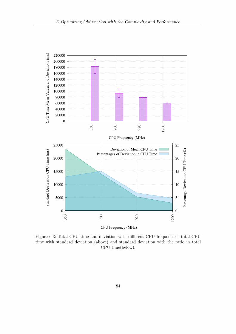
6 Optimizing Obfuscation with the Complexity and Performance
0
20000
40000
60000
80000
100000
120000
140000
160000
180000
200000
220000
350
700
920
1200
CPU
Tim
e M
ean
Val
ues
and
Dev
iatio
ns (m
s)
CPU Frequency (MHz)
0
5000
10000
15000
20000
25000
350
700
920
1200
0
5
10
15
20
25
Stan
dard
Dev
ivat
ion
CPU
Tim
e (m
s)
Perc
enta
ge D
eviv
atio
n C
PU T
ime
(%)
CPU Frequency (MHz)
Deviation of Mean CPU TimePercentages of Deviation in CPU Time
Figure 6.3: Total CPU time and deviation with different CPU frequencies: total CPUtime with standard deviation (above) and standard deviation with the ratio in total
CPU time(below).
84

6 Optimizing Obfuscation with the Complexity and Performance
find out to which value we should fix the frequency since there are several Hz levels thatcan be chosen.
To find the desirable value with the highest accuracy in performance measurement, weperformed some experiments on our target experiment device Samsung Galaxy S II (GT-I9100, CPU Exynos 4210 dual-core max 1.2GHz, 32/32 KB I/D Cache, 1 MB L2 Cache,1G RAM, 16G storage, OS Android 5.1.1.). We use alarmclock.apk as an example, andran this APK 20 times under different CPU frequency (ranging from 350 MHz to 1200MHz). We recorded the averages and standard deviation of the CPU time. The resultsare shown in Figure 6.3.
In this Figure, the graph on the top shows the averages and deviations of the consumedCPU cycles (y-axis) with the available frequencies (x-axis). From this graph, we can seethat the number of used CPU cycles decreases with the increase of the frequency. Moreimportantly, the standard deviation decreases. The graph at the bottom of Figure 6.3shows the ratio of the total consumed CPU cycles for each frequency. The ratio is 12.8%(350MHz) and drops to 4.9% (1200MHz). To minimize the deviations stemming fromfrequency variations of the CPU, we fixed the frequency to 1200MHz, which is also themaximum we can choose on our testing device. Moreover, to have stable performancedata for each result APK, we measured them for 5 times, and calculated the averages.
6.5.3 The Problem of GUI Traversal
In our framework, we use Pandora as an obfuscation engine. Its obfuscation process willcover all the Java methods in every Activity within the target Android applications. Soif we only invoke the MainActivity of the those apps, the majority part of obfuscatedJava methods might be excluded from performance change measurement. Therefore, toaccurately measure the performance loss made by obfuscation, our testing should coveras many Java methods as possible in the target apps.
In Android, a GUI is almost everything a user can see and interact with. An Androidapp is composed by one or more GUIs (as the frontend) and all the supporting Javamethods for these GUIs (as the backend). A collection of those GUIs can be formulatedas a tree graph representing the app. Each node is a visible instance of the GUI itselfand the edges are the connections between the current GUI state and the next, whichare defined by GUI manipulations, e.g. by clicking a button. The starting node of thetree graph is the GUI at the entry point of the MainActivity. We disregard apps whichonly run as services in the background.
To increase the coverage of Java methods for the APKs we measured, we developed atool that performed a “Depth-first with one step back” search of the GUI tree graphby clicking buttons. If the tool reaches a leaf node and cannot go any further, or ifall the buttons in a particular GUI have been clicked already, the tool will press theback button. During the process of traversing the GUI, our tool logs every GUI element(which is the button) it has clicked. The tool then generates a log file for the target app.
85

6 Optimizing Obfuscation with the Complexity and Performance
To implement the performance measurements, we generated such log files for each APKin our measurement set. We use monkeyrunner to replicate the same GUI traversal forboth cleartext APK and obfuscated APK. In both runs we measured and calculated thesum of the CPU time of each Java method. The performance overhead can then bequantified as the additional amount of CPU time caused by the obfuscation.
6.6 The Performance Cost of Obfuscation
Using our framework we can generate different versions of programs with (almost) ar-bitrary target complexity. We are also able to measure the performance cost of thesetransformations and even use performance as a target metric in the search. This allowsus to empirically study the relationship between obfuscation techniques and softwarecomplexity metrics on the one hand, and the relationships of the two concepts withperformance cost on the other hand.
In the following, we first study the performance cost from the obfuscation processeswhen the framework targets specific complexity metrics (Section 6.6.1). Then we in-vestigate the relationship between performance cost and the obfuscation methods. Wewish to find out which obfuscation methods are the most costly in terms of performance(Section 6.6.2).
6.6.1 The Performance Cost when Framework Targets Different SoftwareComplexity Metrics
The effect of certain obfuscation techniques in relation to different software metrics canbe classified into idempotent and monotonous as described in Chapter 5. Intuitively,monotonous techniques cause an increase in the complexity value with every (repeated)obfuscation step. An idempotent technique causes a change in the metric only once(usually in the first invocation). As mentioned above, we only consider the methodmetrics that are monotonous regarding the chosen complexity metrics in our framework.
To investigate the performance cost when our obfuscation framework targets variousmetrics and different complexity values, we performed the following experiment with asample size of 100 APKs which are randomly selected from the F-Droid [35]. Firstly,we set our obfuscation framework to increase the three method metrics (DepDegree,LOC, Cyclomatic) to values of 30%, 50%, 100%, and 150%. Then we measure theextra performance costs made by the obfuscation. We use the 5% trimmed means. Theaverages and standard deviations of the performance cost are listed in Table 6.2. Forexample, a 30% target increase value of the metric DepDegree in our framework causesan average of 16% increase in performance cost (with a standard deviation of 0.33). Afterthat, we performed one-way ANOVA tests among those target complexity values (from30% to 150%) for every metric. The oneway ANOVA test is used to test whether theaverage value of the samples in the four groups are significantly different (null hypothesis
86

6 Optimizing Obfuscation with the Complexity and Performance
H0). If the null hypothesis is rejected, then the performance cost of obfuscation can beinfluenced by the increased target values (from 30% to 150%). More precisely, the nullhypothesis H0 and alternative hypothesis H1 are as follows:
H0: The increase of target complexity values does not influence the performanceaverage.
H1: The increase of target complexity values influences the performance average.
The results of the test are shown on the right side of Table 6.2. Overall, the null hypoth-esis is rejected only for DepDegree (p 0.05). This means that increasing the targetvalue of DepDegree has a statistically significant influence on the average performancecost. For LOC and Cyclomatic we cannot reject H0, which means that we can merelyobserve their performance cost increases but we cannot prove that they are significantlyaffected by the increases of target complexity values.
Table 6.2 also shows which of the metrics is the most performance expensive metric inour framework: For all complexity value increases of the three metrics, Cyclomatic al-ways causes the highest performance cost (47% up to 67%). For increases of complexityvalue below 100%, the “cheapest” metric in terms of performance cost is DepDegree.For 100% increase and above, LOC incurs the least performance cost. To confirm thisobservation, we did one-way ANOVA test to compare the influence of a particular com-plexity metric on the performance average. We did this for the four complexity metricincreases described above (30% to 150%). The results are all significant. Therefore, toachieve the same metric value increase, choosing different complexity metric significantlyaffects the performance cost.
We now discuss these results in more details by looking at the histograms of individualmeasurements from Figures 6.4 to 6.6 and from Figures 6.7 to 6.10.
The three different metrics and their performance costs are shown in the three graphsin Figure 6.4, Figure 6.5, and Figure 6.6. In these graphs, each of the same coloredhistograms, which are in blue, red, purple, or green, represents the performance cost dis-tribution made by the three metrics with different target increase values of 30%, 50%,100%, or 150%. For example, the blue histograms are the performance cost distribu-tions when our framework targets the 30% increases of the metric DepDegree, LOC, orCyclomatic, which are respectively in Figure 6.4, Figure 6.5, and Figure 6.6. With thosethree metric values varying from 30% to 150%, the histograms — colored from blue togreen — are overall increasingly stretched to the right.
To make them more comparable to each other, we also display the Gaussian fit curvescolored the same with the corresponding histogram. The x-value of the peak of the curveis the average value of the histogram, and the extension degree (“the stretch”) along thex-axis of the fit curve can be used to compare the standard deviations (the longer thestretch, the larger the standard deviation).
For example, metric DepDegree is described in Figure 6.4. From 30% to 150%, theaverage values are 0.1681 (in blue curve peak x-value), 0.2310 (in red), 0.3908 (in purple),
87

6 Optimizing Obfuscation with the Complexity and Performance
and 0.5512 (in green), respectively, as shown in the first row of Table 6.2. In this table,from the 50% metric value increase of DepDegree, the average performance costs willbasically increase linearly by around 0.16 when the metric values increase every 50%.Along with the averages, the standard deviations are also increasing.
Figure 6.5 shows the correlations between the Lines of Codes (LOC) and the perfor-mance: We can observe that the histograms and the Gaussian fit curves are rathersimilar and the average performance cost at 30% metric increase is slightly higher thanthat of 50% with the value 0.0344. And their standard deviations differ by 0.0646. How-ever, the 30% increase and the 50% are very close to each other that their averages onlydiffer by 0.0228, and that deviations differ by 0.0009. Therefore, in the second graph,we can also observe that the blue curve basically overlaps with the purple. Meanwhile,the red curve is stretching more to the left comparing to both of the blue and purple.But from 50% to 150%, each step of metric increase has around 0.05 more of averageperformance cost, which is much less than that of DepDegree. As shown in this graph,the x-value of the peaks from of the red, the purple to the green curves steadily increasewith a small amount.
In Figure 6.6, the extra performance overhead of the metric Cyclomatic is shown. Fromthe 30% to 100%, the growing rate is relatively low. From 100% to 150% the performanceaverage increases by 0.1391 to 0.6786. Therefore the peaks of blue, red, purple curves arerelatively close to each other. The green is distinctively further to the positive directionof the x-axis.
We now discuss in more details the four measurement samples for the four classes ofcomplexity metric increase (30% to 150%). The histograms together with the Gaussianfit curves for these four cases are shown From Figure 6.7 to Figure 6.10. Each of thegraph in figure describes the distributions of the three complexity metrics when theirmetric increase values fix to a ratio, for example, Figure 6.7 describes the distributiondifferences of the metrics DepDegree, LOC, and Cyclomatic with 30% metric increases.It allows us to compare the performance cost of different complexity metrics for the samelevel of increase. In this figure, the blue histograms and curves represent DepDegree,the red represent LOC, and the purple represent Cyclomatic. From each of graphs,we intuitively observe that the purple curve (Cyclomatic) always stretches out furthestto the x-axis positive direction. It means Cyclomatic is always the most expensivein performance cost when targeting the same metric value increase. But according toTable 6.2, the difference in average performance cost between Cyclomatic (purple) andDepDegree (blue) gets smaller with larger complexity metric increases (from 0.31 for 30%to 0.12 for 150%). Thus, in the four graphs, we can observe that the blue curves and thepurple curves get closer from the top left to the bottom right. In the first two graphs (formetric value increase of 30% and 50%), the performance cost average of the DepDegree(blue) is lower than that of LOC (red). However, starting from 100% metric valueincrease (Figure 6.9) it is the other way round. Therefore, from Figure 6.9, the peaksx-values of blue curves exceed that of red. It means that the increase of performance costof DepDegree outpaces that of LOC when our framework targets 100% metric increase
88

6 Optimizing Obfuscation with the Complexity and Performance
Tab
le6.
2:P
erfo
rman
ceco
stof
reac
hin
gp
arti
cula
rco
mp
lexit
ym
etri
cin
crea
ses
(n
100)
.
Met
rics
AV
G&
ST
D30
%50
%10
0%15
0%A
NO
VA
f-va
lue
p-v
alue
Dep
Deg
ree
AV
G0.
1681
0.23
100.
3908
0.55
1212
.977
64.
3071
e-08
ST
D0.
3325
0.43
460.
4803
0.60
50
LO
CA
VG
0.31
580.
2814
0.33
860.
3881
0.76
770.
5126
ST
D0.
5338
0.46
920.
5347
0.48
29
Cycl
omat
icA
VG
0.47
450.
4893
0.53
950.
6786
2.22
830.
0844
ST
D0.
6286
0.52
870.
5976
0.70
42
AN
OV
Af-
valu
e8.
9296
7.78
383.
2601
5.65
26p-v
alue
0.00
010.
0005
0.03
990.
0039
89

6 Optimizing Obfuscation with the Complexity and Performance
0.5 0.0 0.5 1.0 1.5 2.0
CPU-Time increase
0.0
0.5
1.0
1.5
2.0
2.5
3.0
3.5
Pro
babili
ty D
ensi
ty
Metrics and Performance DepDegree
fit-dep-0.30fit-dep-0.50fit-dep-1.00fit-dep-1.50hist-dep-0.30hist-dep-0.50hist-dep-1.00hist-dep-1.50
Figure 6.4: Performance overhead increase histogram and the fit curves within the metricsDepDegree with target increase 30%, 50%, 100%, and 150%
0.5 0.0 0.5 1.0 1.5 2.0
CPU-Time increase
0.0
0.5
1.0
1.5
2.0
Pro
babili
ty D
ensi
ty
Metrics and Performance Loc
fit-loc-0.30fit-loc-0.50fit-loc-1.00fit-loc-1.50hist-loc-0.30hist-loc-0.50hist-loc-1.00hist-loc-1.50
Figure 6.5: Performance overhead increase histogram and the fit curves within the metricsLOC with target increase 30%, 50%, 100%, and 150%
90

6 Optimizing Obfuscation with the Complexity and Performance
0.5 0.0 0.5 1.0 1.5 2.0
CPU-Time increase
0.0
0.5
1.0
1.5
2.0
Pro
babili
ty D
ensi
ty
Metrics and Performance Cyclomatic
fit-cyc-0.30fit-cyc-0.50fit-cyc-1.00fit-cyc-1.50hist-cyc-0.30hist-cyc-0.50hist-cyc-1.00hist-cyc-1.50
Figure 6.6: Performance overhead increase histogram and the fit curves within the metricsCyclomatic with target increase 30%, 50%, 100%, and 150%
0.5 0.0 0.5 1.0 1.5 2.0 2.5 3.0 3.5 4.0
CPU-Time increase
0.0
0.2
0.4
0.6
0.8
1.0
1.2
1.4
1.6
1.8
Pro
babili
ty D
ensi
ty
Metrics and Performance 30%
fit-dep-0.30fit-loc-0.30fit-cyc-0.30hist-dep-0.30hist-loc-0.30hist-cyc-0.30
Figure 6.7: Performance overhead increase histogram and the fit curves among the met-rics DepDegree, LOC, and Cyclomatic with target increase 30%
91

6 Optimizing Obfuscation with the Complexity and Performance
0.5 0.0 0.5 1.0 1.5 2.0 2.5 3.0 3.5 4.0
CPU-Time increase
0.0
0.5
1.0
1.5
2.0
Pro
babili
ty D
ensi
ty
Metrics and Performance 50%
fit-dep-0.50fit-loc-0.50fit-cyc-0.50hist-dep-0.50hist-loc-0.50hist-cyc-0.50
Figure 6.8: Performance overhead increase histogram and the fit curves among the met-rics DepDegree, LOC, and Cyclomatic with target increase 50%
0.5 0.0 0.5 1.0 1.5 2.0 2.5 3.0
CPU-Time increase
0.0
0.5
1.0
1.5
2.0
2.5
Pro
babili
ty D
ensi
ty
Metrics and Performance 100%
fit-dep-1.00fit-loc-1.00fit-cyc-1.00hist-dep-1.00hist-loc-1.00hist-cyc-1.00
Figure 6.9: Performance overhead increase histogram and the fit curves among the met-rics DepDegree, LOC, and Cyclomatic with target increase 100%
92

6 Optimizing Obfuscation with the Complexity and Performance
0.5 0.0 0.5 1.0 1.5 2.0 2.5 3.0 3.5
CPU-Time increase
0.0
0.2
0.4
0.6
0.8
1.0
1.2
1.4
Pro
babili
ty D
ensi
ty
Metrics and Performance 150%
fit-dep-1.50fit-loc-1.50fit-cyc-1.50hist-dep-1.50hist-loc-1.50hist-cyc-1.50
Figure 6.10: Performance overhead increase histogram and the fit curves among themetrics DepDegree, LOC, and Cyclomatic with target increase 150%
and hereafter.
6.6.2 The Performance Cost of Obfuscation Methods
We now investigate the performance overhead caused by different obfuscation methods.As mentioned above, we selected 7 obfuscation methods out of 11 because they aremonotonous with respect to the three metrics discussed in Section 6.2.1. The results areshown in Table 6.3.
For DepDegree, the highest average increase is caused by Integer Encoding (0.5885)which causes an extra performance cost of only 0.0789 on average. The second highestaverage increase comes from Compose Locals (0.4750). Its performance penalty howeveris 0.3398, which is almost 5 times of that of Integer Encoding. The performance cost ofString Encryption, though only causing a 0.0746 metric increase, is up to 0.5844. Thisis similar to the effect of Move Methods.
The metric increases and performance penalty for Lines of Code (LOC) are similar tothose of DepDegree. Integer Encoding is the highest in metric change but lowest in theperformance cost. Compose Locals is the second highest regarding metric increase butscores relatively high in performance penalty. String Encryption and Move Methods arerather costly in terms of performance but very low in metric increase.
93

6 Optimizing Obfuscation with the Complexity and Performance
Regarding Cyclomatic the results are quite different from DepDegree and LOC. Here,Encapsulate Fields is the method which changes the metric most (0.2042) and is cheapin performance (0.0450). In this metric most of the average values are below 0.20, whichis less than the previous metrics. So, to reach similar values, more steps of obfuscationare needed. If one relates performance cost to metric increase, Cyclomatic is on averagethe most performance expensive metric.
We now analyze the two obfuscation methods, String Encryption and Compose Locals,in more details. Figure 6.11 shows histograms of the metric increases of String Encryp-tion in our experiments. It shows that most APKs do not change much regarding thethree metrics we considered. The histogram of performance cost, however, does not showa particular peak. Figure 6.12 shows the same graphs for Compose Locals: the metricchanges are comparatively larger and the performance increase shows a peak aroundthe value 0.2. Similar measurements were taken for Integer Encoding. Overall, Inte-ger Encoding and Compose Locals appear to be rather cheap in terms of performanceoverhead.
94

6 Optimizing Obfuscation with the Complexity and Performance
Tab
le6.3
:A
vera
ge
(AV
G)
met
ric
incr
ease
sw
ith
stan
dar
dd
evia
tion
(ST
D)
and
per
form
an
ceov
erh
ead
for
each
ob
fusc
atio
nm
eth
od
(n
100)
Obfu
Met
hods
AV
G&
ST
DStr
Encr
ypt
Int
Enco
de
Com
pL
oca
lE
xtr
act
Met
hM
ove
Met
hE
nca
pF
ield
Mer
geM
eth
Dep
Deg
ree
AV
G0.
0746
0.58
850.
4705
0.06
710.
0503
0.07
310.
0074
ST
D0.
2044
0.32
200.
2124
0.07
550.
0859
0.07
580.
0648
LO
CA
VG
0.04
550.
5730
0.38
440.
1016
0.04
360.
1271
0.00
17ST
D0.
1178
0.35
240.
1851
0.06
820.
0671
0.07
980.
0482
Cycl
omat
icA
VG
0.02
110.
1528
0.19
500.
1312
0.00
500.
2042
0.00
18ST
D0.
0839
0.17
760.
1897
0.09
160.
0639
0.14
950.
0644
Per
form
ance
AV
G0.
5844
0.07
890.
3398
0.03
580.
5196
0.04
500.
0159
ST
D0.
6926
0.16
540.
3675
0.11
160.
9528
0.10
110.
1126
95

6 Optimizing Obfuscation with the Complexity and Performance
0
20
40
60
80
100
120
140
160
180
200
-0.1 -0.05 0 0.05 0.1 0.15 0.2 0.25
Freq
uenc
y
increased metric
depdegreeloc
cyclomatic
0
2
4
6
8
10
12
14
16
-0.2 0 0.2 0.4 0.6 0.8 1 1.2
APK
Num
bers
CPU-Time increased
Figure 6.11: Histogram of the method metric increase and the performance overheadincrease regarding String Encryption.
96

6 Optimizing Obfuscation with the Complexity and Performance
0
10
20
30
40
50
60
70
80
0 0.2 0.4 0.6 0.8 1 1.2
APK
Num
bers
Percentange of Increased Metrics
depdegreeloc
cyclomatic
0
5
10
15
20
25
30
-0.2 0 0.2 0.4 0.6 0.8 1 1.2
APK
Num
bers
CPU-Time increased
Figure 6.12: Histogram of the method metric increase and the performance overheadincrease regarding Compose Locals.
6.6.3 Performance as a Special Metric
Given the fact that some obfuscation methods are cheaper regarding performance thanothers, we can use this insight to create obfuscated programs that reach the same metricvalue increase at a smaller performance overhead. We therefore use the statistical datafrom the previous section in our algorithm based on the Naıve Bayesian Classifier. Weadapted our framework such that the maximum performance overhead could be givenas an additional metric value. For example, we could now start the search for a versionof the program with an increase of DepDegree of 100% but where the performance costshould be limited to a 35% increase.
97

6 Optimizing Obfuscation with the Complexity and Performance
Table 6.4: Performance cost (“perf”) of obfuscated programs resulting from the NaıveBayesian algorithm by limiting performance loss to the average performance increase
(“norm”) of earlier measurements.
Metrics 30% 50% 100% 150%perf norm perf norm perf norm perf norm
DepDegree AVG 0.0172 0.8971 0.0394 0.8853 0.1108 1.0043 0.2112 1.1567STD 0.1039 1.7770 0.0836 1.4309 0.1283 0.7738 0.2063 0.5140
LOC AVG 0.1002 0.8374 0.0840 1.0187 0.1670 1.1973 0.1808 1.2143STD 0.1398 0.7053 0.1054 0.7084 0.1191 1.4624 0.1375 1.2750
Cyclomatic AVG 0.1528 1.5055 0.3202 1.4301 0.4146 1.4508 0.5053 1.9411STD 0.2103 1.1109 0.2361 1.3185 0.2072 0.9974 0.2651 1.5605
Recalling the measurements from Section 6.6.1, we now generated obfuscated versionsof 100 APKs for different metric value increases (from 30% to 150%) and we used theaverage performance cost from the original measurements as a boundary in guiding thesearch. The results are shown in the Table 6.4. For each metric (DepDegree, LOC, Cy-clomatic) the table lists the average performance increase (AVG) and standard deviation(STD) that was measured before performance optimization (“norm”) and contrasts itwith the average performance increase when low performance penalty is used as addi-tional search criterion in the the Naıve Bayesian Classifier algorithm (“perf”). The tableshows that the same metric increase can be achieved with dramatically lower performancecosts. We observe that the ratio between optimized performance increase and “normal”performance increase gets smaller as metric values (of DepDegree, LOC, Cyclomatic)increase. The largest savings in performance can therefore be achieved for small metricvalue increases. For example, at a 30% increase in DepDegree the optimized programruns 50 times faster that the non-optimized version, whereas the narrowest margin takesplace when the metric Cyclomatic is increased to 150%. In this case we are “only” fasterby a factor of 4. Overall, DepDegree can be optimized the most, i.e., it has the highestchance to be optimized regarding performance. Even after performance optimization,Cyclomatic remains the most expensive metric regarding average .
From Figure 6.13 to 6.15, the blue plots are the performance of the result APKs whichare obfuscated respectively to the target metric (DepDegree, LOC, Cyclomatic) andtheir desired values (30%, 50%, 100%, 150%). (e.g. in DepDegree 150%, we select theAPKs with the performance lager than the average value 0.5319 from the Table 6.2.).The red are those same APKs under the performance optimized obfuscation. In thesegraphs, the axis of “Actual Metric Values” are the metric values they have reached afterobfuscation. The “Target Metric Values” in the graphs are the desired values, and thegoal of our obfuscation framework. As we can see in those graphs, all the blue plotsand red plots are basically vertical distributed. For the blue plots, we can see that theymainly concentrate around the axis of target values, but stretched to larger performance
98

6 Optimizing Obfuscation with the Complexity and Performance
values. For instance in the Figure 6.13 (DepDegree), when the target metric values arepointing to 150% (which is the most inside layer of distribution in this graph), the blueplots gather around “Actual Metric Values” of 1.5. Meanwhile, their “Performance”values are getting larger.
Representing the performance optimized APKs, the majority of the red plots are dis-tributed under a certain performance values, which are the average values we acquiredfrom the Table 6.2. Because during the obfuscation process, we do statistics based onall the results performance data from Section 6.6.2, and then use them in our NaıveBayesian Classifier, same as the other complexity metrics. After calculation, we wouldchoose the dominant obfuscation method (which is performance and metric economy) asintroduced in Section 6.4.2. In this way, we can limit the increase in performance costunder the averages.
Before our obfuscation framework is performance optimized, we only confine the com-plexity increase. Because when we obfuscate blindly only by the complexity metrics,the result APKs could be very possibly over obfuscated. It means that the performanceis overburdened by too many increased metrics values (Our theory assumes that morecomplexity metric requires more computing resources). After optimization, the concernof performance overburden is solved. We could set the framework with a performanceoverhead limitation, the result metric could be over the target value and as high as pos-sible. As a result, the red plots in these Figures can be very high in the metric valueswhile limited in performance overhead. We take the same example when DepDegreetargeting 150% in Figure 6.13, the red plots are stretched to the larger values of the“Actual Metric Values” axis, but all of them are below performance values 0.5319 whichis the average of extra performance cost from the Table 6.2. A minimal of the APKscannot reach the 80% or 90% of the target metric values after we use the performanceas another metric for optimization, the ratio of those APKs and the total sample spaceare shown in Table 6.5.
99

6 Optimizing Obfuscation with the Complexity and Performance
Perfo
rman
ce
1
0
1
2
3
4
5
6
Actual Metric Values
0.5 0.0 0.5 1.0 1.5 2.0 2.5 3.0 3.5 4.0
Targ
et M
etric
Val
ues
0.20.40.60.81.01.21.41.6
DepDegree Performance Optimization
Figure 6.13: Plotting of the Performance and DepDegree
Perfo
rman
ce
1
0
1
2
3
4
5
6
Actual Metric Values
0.5 0.0 0.5 1.0 1.5 2.0 2.5 3.0 3.5
Targ
et M
etric
Val
ues
0.20.40.60.81.01.21.41.6
Loc Performance Optimization
Figure 6.14: Plotting of the Performance and LOC
100

6 Optimizing Obfuscation with the Complexity and Performance
Table 6.5: The ratio of the APKs that can NOT reach the 0.8 and 0.9 times targetcomplexity metric values.
Metrics Target Values 30% 50% 100% 150%Range&Total <0.9 <0.8 <0.9 <0.8 <0.9 <0.8 <0.9 <0.8
DepDegree Range 13.5% 2.7% 6.52% 4.35% 5.26% 5.26% 11.36% 11.36%Total 37 46 38 44
LOC Range 33.33% 12.82% 20.69% 13.79% 4% % 2.27% 2.27%Total 39 29 25 44
Cyclomatic Range 52.77% 5% 7.69% 5.13% 16.28% 11.63% 23.91% 18.6%Total 36 39 43 46
Perfo
rman
ce1
0
1
2
3
4
5
6
Actual Metric Values
0.5 0.0 0.5 1.0 1.5 2.0 2.5 3.0
Targ
et M
etric
Val
ues
0.20.40.60.81.01.21.41.6
Cyclomatic Performance Optimization
Figure 6.15: Plotting of the Performance and Cyclomatic
6.7 Conclusion
In this chapter we defined the problem of optimal software obfuscation and empiricallyevaluated two search algorithms for obfuscated versions in the context of Android APKs.With a training set of more than 400 APKs and measurements on 110 APKs, we couldshow that the second algorithm based on the Naıve Bayesian Classifier outperforms asimple greedy search considerably. We also investigated the performance cost of different
101

6 Optimizing Obfuscation with the Complexity and Performance
types of software obfuscation in this context. We showed that some obfuscation methods(like String Encryption) are more performance costly than others to achieve the samemetric value increase. We also found that especially for small metric value increases,large performance benefits can be achieved if the right obfuscation techniques are used,i.e. those that are less costly in terms of performance.
102

Chapter 7
Conclusion
7.1 Summary
In Chapter 4, we have given an overview of the composition and the work flows of ourobfuscation framework, which we define as the process of creating all the optimized resultAPKs in both complexities and performance. It produces all the result in the followingchapters. We have introduced the working principle of the obfuscation methods andsoftware complexity metrics and the classification of the attributes of the methods andthe metrics, which are categorized into the method level (data control flows) and theclass level (Object-Oriented Design). We pointed out the rationale of measuring “diffi-culty” and complex level caused by the obfuscation methods by the software complexitymetrics. We have developed an automatic testing tool to generate the testing cases forperformance analysis. The testing cases refer to the clicking or sliding action used toinvoke the active GUI elements on the testing device. Because the tree based data struc-ture of the GUI elements and the Android activities, the testing tool must implement“Depth-First search with one step back” to traverse the tree, which can cover most of theactive elements, hence achieving the maximum code coverage. The obfuscation manage-ment layer is designed to coordinate and control all the modules in the framework. Weoffered an overview on its mechanism: Based on the learning set data, it will evaluateand apply different obfuscation method for different scenarios.
To further optimize the obfuscation process with complexity metrics, a number of trans-formation results of each obfuscation method need to be analyzed, and used as thelearning set. In Chapter 5, we have given an overview that is based on different transfor-mation theories and mechanisms. The obfuscation methods show different but structuralattributes when evaluated by an array of software complexity metrics. To demonstratethe attributes we have implemented our framework to iteratively apply the same ob-fuscation methods onto the APKs, and evaluated the difference before and after trans-formation with metrics and similarity. Using these proof-of-concept implementations,we have performed the evaluation of 7 obfuscation methods with 9 complexity metrics.We showed from the pictures that the results are rather complex since a single obfus-cation method usually exhibits different properties (i.e. monotonicity or idempotency)and values regarding different complexity metrics. Meanwhile, most of the monotonic-ity obfuscation methods exhibit a rather “stable” attribute, that complexity value risesconstantly by a certain ratio after each iteration. However, a few obfuscation methodsdemonstrate unstable properties regarding some of the metrics. The analysis of the ob-fuscation methods properties is the basis of our further research, which is to optimizethe APKs to the designated metrics with minimum obfuscation iterations.
103

7 Conclusion
In Chapter 6, we define an obfuscation as “successful” when it transforms the APK toa certain level of “difficulty”, without significantly slowing it down. Instead of the ab-stract “difficulty” level, we use software complexity metrics values to measure concreteobfuscation results. To reach these concrete metrics values, we implement algorithms,which are either the Naıve Bayes Classifier or the mean values based simple search, inthe Obfuscation Management Layer of the framework to guide the obfuscation processto select the suitable obfuscation methods. The algorithms determine which method touse according to the complexity metrics data of the learning set from obfuscation history.By comparing the results of the two algorithms, the Naıve Bayes Classifier outperformsthe mean values based simple search. We then use the Naıve Bayes Classifier to guidethe obfuscation methods selections to optimize the complexity metrics into target val-ues and confine the performance penalty. To start the performance measurement, weimplement the performance measurement modules in the framework during obfuscationprocess. We have evaluated performance penalty of different obfuscated methods andalso that in relation to three metrics at different increased complexity values, i.e. De-pDegree, LOC, Cyclomatic Complexity. Our evaluation showed that DepDegree is themost performance saving metric while having the same target metric values as Cyclo-matic Complexity, which is the most performance expensive metric. Meanwhile, someof the obfuscation methods are significantly more costly in performance than otherswhen the metric value changes are similar, i.e. Strings Encryption, Compose Locals,and Move Methods. Therefore we conclude that, considering performance as a specifictarget metric during obfuscation, the Obfuscation Management Layer in our frameworkwill produce the result APKs with far lower performance cost, meanwhile satisfying thetarget complexity metrics.
7.2 Future Work
While the techniques we have developed in this thesis have extended optimized obfus-cation from complexity to performance, there is still potential for further research. Tomaintain user experience after obfuscation, the Obfuscation Management Layer can sta-tistically guide the obfuscation methods selection in the transformation process withthe minimum performance cost. However, in mobile devices, not only performance, butenergy consumption is also an important criterion for the user. Because obfuscationtransformation causes more complexity for the software, more computing power is con-sumed. Measured by the CPU cycles, performance expenses generated by obfuscationcannot fully reflect extra power consumptions. Therefore, it is necessary to measure andprofile the energy consumption for the target application. The hardware based energyprofiling toolset, the Monsoon power monitor [94], for example, can be implemented tomeasure energy consumption more exactly than the power modeling or estimation soft-ware [48, 68, 47]. Because the Monsoon power monitor is only an energy measurementtool, we then need to align its time indexed energy consumption curves exactly to ourperformance profiling results in order to show accurately the time schedule of each Javamethod. As a result, we could investigate the correlation between energy consumption
104

7 Conclusion
and different obfuscation methods or complexity metrics at different values.
Furthermore, we suggest researching on the correlation between complexity metrics val-ues and the “difficulty” level from the human perspective. While this approach is muchmore complicated, it is interesting to know to what extent complexity values add “dif-ficulty” to reverse engineer the software. This can provide a more accurate complexitytarget to guide our obfuscation process.
105


Bibliography
[1] LLVM. http://llvm.org/, 2007.
[2] Dex2jar. https://sourceforge.net/projects/dex2jar/, 2009.
[3] Snappy. https://github.com/google/snappy, 2011.
[4] apk-view-tracer. https://code.google.com/archive/p/apk-view-tracer/,2012.
[5] Profiling with traceview and dmtracedump. https://developer.android.com/
studio/profile/traceview.html#traceviewLayout, 2012.
[6] IDA Pro homepage. https://www.hex-rays.com/products/ida/index.shtml,2015.
[7] ISO/IEC 9126-2. Software engineering – product quality – part 2: External met-rics. ISO/IEC, June 2001.
[8] Ivan Arce and Elias Levy. An analysis of the slapper worm. IEEE Security &Privacy, 1(1):82–87, 2003.
[9] John Aycock. Computer Viruses and Malware, volume 22 of Advances in Infor-mation Security. Springer, 2006.
[10] Barak, Goldreich, Impagliazzo, Rudich, Sahai, Vadhan, and Yang. On the(im)possibility of obfuscating programs. In CRYPTO: Proceedings of Crypto, 2001.
[11] Boaz Barak, Oded Goldreich, Russell Impagliazzo, Steven Rudich, Amit Sahai,Salil P. Vadhan, and Ke Yang. On the (im)possibility of obfuscating programs. J.ACM, 59(2):6, 2012.
[12] Victor R. Basili and Barry T. Perricone. Software errors and complexity: Anempirical investigation. Commun. ACM, 27(1):42–52, 1984.
[13] Philippe Beaucamps. Advanced metamorphic techniques in computer viruses. Au-thor manuscript, published in ”International Conference on Computer, Electrical,and Systems Science, and Engineering - CESSE’07 (2007), November 14 2008.
[14] M. Becher, F. C. Freiling, and B. Leider. On the effort to create smartphoneworms in windows mobile. In 2007 IEEE SMC Information Assurance and SecurityWorkshop, pages 199–206, June 2007.
[15] Michael Becher. Security of Smartphones at the Dawn of Their Ubiquitousness.Phd thesis, University of Mannheim, Germany, 2009.
107

Bibliography
[16] Boldizsar Bencsath, Gabor Pek, Levente Buttyan, and Mark Felegyhazi. Thecousins of stuxnet: Duqu, flame, and gauss. Future Internet, 4(4):971–1003, 2012.
[17] Dirk Beyer and Ashgan Fararooy. Depdigger: A tool for detecting complex low-level dependencies. International Conference on Program Comprehension, 00:40–41, 2010.
[18] Hamad Binsalleeh, Thomas Ormerod, Amine Boukhtouta, Prosenjit Sinha,Amr M. Youssef, Mourad Debbabi, and Lingyu Wang. On the analysis of thezeus botnet crimeware toolkit. In PST, pages 31–38. IEEE, 2010.
[19] Bitdefender. Malware history. Technical report, 2008.
[20] Abhijit Bose, Xin Hu, Kang G. Shin, and Taejoon Park. Behavioral detection ofmalware on mobile handsets. In Dirk Grunwald, Richard Han, Eyal de Lara, andCarla Schlatter Ellis, editors, MobiSys, pages 225–238. ACM, 2008.
[21] Ran Canetti and Ronny Ramzi Dakdouk. Obfuscating Point Functions with Multi-bit Output. In EUROCRYPT ’08 (Proceedings of the theory and applicationsof cryptographic techniques 27th annual international conference on Advances incryptology), pages 489–508, Istanbul, Turkey, April 2008. Springer-Verlag, Berlin.
[22] Mariano Ceccato, Andrea Capiluppi, Paolo Falcarin, and Cornelia Boldyreff. Alarge study on the effect of code obfuscation on the quality of java code. EmpiricalSoftware Engineering, 20(6):1486–1524, 2015.
[23] Mariano Ceccato, Massimiliano Penta, Paolo Falcarin, Filippo Ricca, MarcoTorchiano, and Paolo Tonella. A family of experiments to assess the effectivenessand efficiency of source code obfuscation techniques. Empirical Software Engineer-ing, pages 1–35, 2013.
[24] Mariano Ceccato, Massimiliano Di Penta, Jasvir Nagra, Paolo Falcarin, FilippoRicca, Marco Torchiano, and Paolo Tonella. Towards experimental evaluation ofcode obfuscation techniques. In Andy Ozment and Ketil Stølen, editors, QoP,pages 39–46. ACM, 2008.
[25] Mariano Ceccato, Massimiliano Di Penta, Jasvir Nagra, Paolo Falcarin, FilippoRicca, Marco Torchiano, and Paolo Tonella. The effectiveness of source code ob-fuscation: An experimental assessment. In ICPC, pages 178–187, 2009.
[26] Silvio Cesare and Yang Xiang. Classification of malware using structured con-trol flow. In Proceedings of the Eighth Australasian Symposium on Parallel andDistributed Computing - Volume 107, AusPDC ’10, pages 61–70, Darlinghurst,Australia, Australia, 2010. Australian Computer Society, Inc.
[27] Cilibrasi and Vitani. Clustering by compression. IEEETIT: IEEE Transactionson Information Theory, 51, 2005.
108

Bibliography
[28] Christian Collberg and Jasvir Nagra. Surreptitious Software: Obfuscation, Water-marking and Tamperproofing for Software Protection. Addison-Wesley Longman,Amsterdam, July 2009.
[29] Christian Collberg, Clark Thomborson, and Douglas Low. A taxonomy of obfus-cating transformations. Technical Report 148, Department of Computer Sciences,The University of Auckland, July 1997.
[30] Jedidiah R. Crandall, Roya Ensafi, Stephanie Forrest, Joshua Ladau, and BilalShebaro. The ecology of malware. In Matt Bishop, Christian W. Probst, Angelos D.Keromytis, and Anil Somayaji, editors, NSPW, pages 99–106. ACM, 2008.
[31] Jonathan Crussell, Clint Gibler, and Hao Chen 0003. Attack of the clones: De-tecting cloned applications on android markets. In Sara Foresti, Moti Yung, andFabio Martinelli, editors, ESORICS, volume 7459 of Lecture Notes in ComputerScience, pages 37–54. Springer, 2012.
[32] Bill Curtis, Sylvia B. Sheppard, and Phil Milliman. Third time charm: Strongerprediction of programmer performance by software complexity metrics. In Pro-ceedings of the 4th International Conference on Software Engineering, ICSE ’79,pages 356–360, Piscataway, NJ, USA, 1979. IEEE Press.
[33] Tom deMarco. Controlling Software Projects: Management, Measurement, andEstimates. Springer-Verlag, 1986.
[34] Anthony Desnos. Androguard. https://code.google.com/p/androguard/, 2012.
[35] F-Droid Ltd. F-droid. https://f-droid.org/, 2010.
[36] F-Secure. Bluetooth-worm:symbos/cabir. http://www.f-secure.com/v-descs/cabir.shtml, 2004.
[37] F-Secure. Virus:w32/duts.1520. http://www.f-secure.com/v-descs/dtus.shtml,2004.
[38] Rik Ferguson. The botnet chronicles. Technical report, Trend Micro, Incorporated,2010.
[39] Peter Szor Frdric Perriot. An analysis of the slapper worm exploit. Technicalreport, Symantec Security Response, 2003.
[40] Felix C. Freiling, Mykola Protsenko, and Yan Zhuang. An empirical evaluationof software obfuscation techniques applied to Android APKs. In InternationalWorkshop on Data Protection in Mobile and Pervasive Computing (DAPRO 2014),2014.
[41] Sanjam Garg, Craig Gentry, Shai Halevi, Mariana Raykova, Amit Sahai, and BrentWaters. Candidate indistinguishability obfuscation and functional encryption forall circuits. IACR Cryptology ePrint Archive, 2013:451, 2013.
109
Bibliography
[42] Craig Gentry. Fully Homomorphic Encryption Using Ideal Lattices. In Proceedingsof the Forty-first Annual ACM Symposium on Theory of Computing, STOC ’09,pages 169–178, New York, NY, USA, 2009. ACM.
[43] Roberto Giacobazzi and Isabella Mastroeni. Making abstract interpretation incom-plete: Modeling the potency of obfuscation. In Proceedings of the 19th Interna-tional Conference on Static Analysis, SAS’12, pages 129–145, Berlin, Heidelberg,2012. Springer-Verlag.
[44] Alexander Gostev. Mobile malware evolution: An overview, part 1.http://www.securelist.com/en/analysis?pubid=200119916, 2006.
[45] Alexander Gostev. Mobile malware evolution: An overview, part 2.http://www.securelist.com/en/analysis?pubid=201225789, 2006.
[46] Steve Hanna, Ling Huang, Edward XueJun Wu, Saung Li, Charles Chen, andDawn Song. Juxtapp: A scalable system for detecting code reuse among androidapplications. In Ulrich Flegel, Evangelos P. Markatos, and William K. Robertson,editors, DIMVA, volume 7591 of Lecture Notes in Computer Science, pages 62–81.Springer, 2012.
[47] Shuai Hao, Ding Li, William G. J. Halfond, and Ramesh Govindan. Estimatingandroid applications’ CPU energy usage via bytecode profiling. In Rick Kaz-man, Patricia Lago, Niklaus Meyer, Maurizio Morisio, Hausi A. Muller, FrancesPaulisch, Giuseppe Scanniello, and Olaf Zimmermann, editors, GREENS, pages1–7. IEEE, 2012.
[48] Shuai Hao, Ding Li, William G. J. Halfond, and Ramesh Govindan. Estimatingmobile application energy consumption using program analysis. In David Notkin,Betty H. C. Cheng, and Klaus Pohl, editors, ICSE, pages 92–101. IEEE ComputerSociety, 2013.
[49] Thorsten Holz, Markus Engelberth, and Felix C. Freiling. Learning more aboutthe underground economy: A case-study of keyloggers and dropzones. In MichaelBackes and Peng Ning, editors, ESORICS, volume 5789 of Lecture Notes in Com-puter Science, pages 1–18. Springer, 2009.
[50] Heqing Huang, Sencun Zhu, Peng Liu, and Dinghao Wu. A framework for evalu-ating mobile app repackaging detection algorithms. In Michael Huth, N. Asokan,Srdjan Capkun, Ivan Flechais, and Lizzie Coles-Kemp, editors, TRUST, volume7904 of Lecture Notes in Computer Science, pages 169–186. Springer, 2013.
[51] R. Jain. The art of computer systems performance analysis. SIGMETRICS Per-formance Evaluation Review, 18(3):21–22, 1990.
[52] Dennis G. Kafura and Geereddy R. Reddy. The use of software complexity metricsin software maintenance. IEEE Transactions on Software Engineering, 13(3):335–343, March 1987.
110

Bibliography
[53] Stephen H. Kan. Metrics and Models in Software Quality Engineering. Addison-Wesley Longman Publishing Co., Inc., Boston, MA, USA, 2nd edition, 2002.
[54] Taghi M. Khoshgoftaar and John C. Munson. Predicting software developmenterrors using software complexity metrics. IEEE Journal on Selected Areas in Com-munications, 8(2):253–261, 1990.
[55] Donald E. Knuth. The Art of Computer Programming, Volume II: SeminumericalAlgorithms, 2nd Edition. Addison-Wesley, 1981.
[56] D. Krishnaswamy, R. N. Hasbun, and J. P. Brizek. Secure manageable mobilehandset platform architectures. Comm. Mag., 44(9):158–165, September 2006.
[57] Byoungyoung Lee, Long Lu, Tielei Wang, Taesoo Kim, and Wenke Lee. Fromzygote to morula: Fortifying weakened ASLR on android. In IEEE Symposium onSecurity and Privacy, pages 424–439. IEEE Computer Society, 2014.
[58] Anirban Majumdar, Stephen Drape, and Clark D. Thomborson. Slicing obfus-cations: design, correctness, and evaluation. In Moti Yung, Aggelos Kiayias, andAhmad-Reza Sadeghi, editors, Digital Rights Management Workshop, pages 70–81.ACM, 2007.
[59] Denis Maslennikov. ZeuS-in-the-Mobile Facts and Theories. 2011.
[60] Daniel A. Menasce, Lawrence W. Dowdy, and Virgilio A. F. Almeida. Performanceby Design: Computer Capacity Planning By Example. Prentice Hall PTR, UpperSaddle River, NJ, USA, 2004.
[61] Jonathan Meyer and Daniel Reynaud. Jasmin. http://jasmin.sourceforge.
net/, 2004.
[62] Trend Micro. Repeating history. Technical report, 2012.
[63] Michael Miller. Absolute PC Security and Privacy. 2002.
[64] Carey Nachenberg. Computer virus-antivirus coevolution. Commun. ACM,40(1):46–51, January 1997.
[65] Eric Chien Nicolas Falliere. Zeus: King of the bots. Technical report, Symantec,2009.
[66] Hilarie K. Orman. The morris worm: A fifteen-year perspective. IEEE Security& Privacy, 1(5):35–43, 2003.
[67] Abhinav Pathak, Y. Charlie Hu, and Ming Zhang. Where is the energy spentinside my app?: fine grained energy accounting on smartphones with eprof. InPascal Felber, Frank Bellosa, and Herbert Bos, editors, EuroSys, pages 29–42.ACM, 2012.
111

Bibliography
[68] Abhinav Pathak, Y. Charlie Hu, Ming Zhang, Paramvir Bahl, and Yi-Min Wang.Fine-grained power modeling for smartphones using system call tracing. InChristoph M. Kirsch and Gernot Heiser, editors, EuroSys, pages 153–168. ACM,2011.
[69] Phillip A. Porras, Hassen Saıdi, and Vinod Yegneswaran. An analysis of theikee.B iphone botnet. In Andreas U. Schmidt, Giovanni Russello, Antonio Lioy,Neeli R. Prasad, and Shiguo Lian, editors, MobiSec, volume 47 of Lecture Notes ofthe Institute for Computer Sciences, Social Informatics and TelecommunicationsEngineering, pages 141–152. Springer, 2010.
[70] Pouik and G0rfi3ld. Similarities for fun and profit. http://phrack.org/issues/68/15.html, April 2014.
[71] Mila Dalla Preda and Roberto Giacobazzi. Semantic-based code obfuscation by ab-stract interpretation. In ICALP: Annual International Colloquium on Automata,Languages and Programming, 2005.
[72] Mila Dalla Preda and Roberto Giacobazzi. Semantics-based Code Obfuscationby Abstract Interpretation. Journal of Computer Security (JCS), 17(6):855–908,2009.
[73] Mila Dalla Preda, Roberto Giacobazzi, Matias Madou, and Koen De Bosschere.Opaque predicates detection by abstract interpretation, 2006.
[74] Mykola Protsenko and Tilo Muller. Pandora applies non-deterministic obfuscationrandomly to android. In MALWARE, pages 59–67. IEEE, 2013.
[75] Niels Provos, Dean McNamee, Panayiotis Mavrommatis, Ke Wang, and NagendraModadugu. The ghost in the browser: Analysis of web-based malware. In FirstWorkshop on Hot Topics in Understanding Botnets, HotBots’07. USENIX, 2007.
[76] Krishna K. Ramachandran and Biplab Sikdar. Modeling malware propagationin networks of smart cell phones with spatial dynamics. In INFOCOM, pages2516–2520. IEEE, 2007.
[77] Vaibhav Rastogi, Yan Chen, and Xuxian Jiang. Droidchameleon: Evaluating an-droid anti-malware against transformation attacks, July 15 2013.
[78] S. Russel and P. Norvig. Artificial Intelligence: A Modern Approach. Prentice-Hall,1995.
[79] Antonino Sabetta and Heiko Koziolek. Measuring performance metrics: Tech-niques and tools. In Irene Eusgeld, Felix C. Freiling, and Ralf H. Reussner, editors,Dependability Metrics, volume 4909 of Lecture Notes in Computer Science, pages226–232. Springer, 2005.
112

Bibliography
[80] Sebastian Schrittwieser, Stefan Katzenbeisser 0001, Johannes Kinder, Georg Merz-dovnik, and Edgar R. Weippl. Protecting software through obfuscation: Can itkeep pace with progress in code analysis? ACM Comput. Surv, 49(1):4, 2016.
[81] SECURELIST. Trojan.symbos.mosquit.a. http://www.securelist.com/ en/de-scriptions/old58141, 2004.
[82] V. Y. Shen, T. J. Yu, S. M. Thebaut, and L. R. Paulsen. Identifying error-pronesoftware - an empirical study. IEEE Transactions on Software Engineering, SE-11(4):317–25, 1985.
[83] Rich Skrenta. Elk cloner. http://www.skrenta.com/cloner/, 2013.
[84] Connie U. Smith and Lloyd G. Williams. Performance solutions: A practical guideto creating responsive, scalable software. In Int. CMG Conference, pages 355–358.Computer Measurement Group, 2001.
[85] Yingbo Song, Michael E. Locasto, Angelos Stavrou, Angelos D. Keromytis, andSalvatore J. Stolfo. On the infeasibility of modeling polymorphic shellcode - re-thinking the role of learning in intrusion detection systems. Machine Learning,81(2):179–205, 2010.
[86] Michael Spreitzenbarth. Dissecting the Doid: Forensic Analysis of Android and itsMalicious Applications. Phd thesis, Department of Computer Science, Friedrich-Alexander-University, Erlangen, Germany, 2013.
[87] State. review of bruen forcinito, cryptography, information theory, and error-correction: A handbook for the 21st century (wiley-interscience, 2004). COM-PREVS: ACM Computing Reviews, 47, 2006.
[88] symantec. Dialer.trojan. http://www.symantec.com/security_response/
writeup.jsp?docid=2001-010916-4630-99. January, 2001.
[89] symantec. Wince.pmcryptic. http://www.symantec.com/connect/blogs/
smart-worm-smartphone-wincepmcryptica. last accessed: March 25, 2013.
[90] Symantec. Backdoor. brador. a. http://www.symantec.com/securityresponse/writeup.jsp?docid=2004-080516-3455-99&tabid=2, 2004.
[91] Ken Thompson. Reflections on trusting trust. chapter Reflections on trustingtrust. ACM, New York, NY, USA, 2007.
[92] Raja Vallee-Rai. Soot: A java bytecode optimization framework, 2000.
[93] Raja Vallee-Rai, Etienne Gagnon, Laurie J. Hendren, Patrick Lam, Patrice Pom-inville, and Vijay Sundaresan. Optimizing Java bytecode using the Soot framework:Is it feasible? In Compiler Construction, 9th International Conference (CC 2000),pages 18–34, 2000.
113

Bibliography
[94] Mario Linares Vasquez, Gabriele Bavota, Carlos Bernal-Cardenas, Rocco Oliveto,Massimiliano Di Penta, and Denys Poshyvanyk. Mining energy-greedy API usagepatterns in android apps: an empirical study. In Premkumar T. Devanbu, SungKim, and Martin Pinzger, editors, MSR, pages 2–11. ACM, 2014.
[95] A. Watson and T. McCabe. Structured testing: A testing methodology using thecyclomatic complexity metric. Technical report, National Institute of Standardsand Technology, Washington, D.C., 1996.
[96] Hoeteck Wee. On Obfuscating Point Functions. In STOC ’05 (Proceedings of thethirty-seventh annual ACM symposium on Theory of computing), pages 523–532,Baltimore, MD, USA, April 2005. ACM, NY.
[97] Cui Xiang, Fang Binxing, Yin Lihua, Liu Xiaoyi, and Zang Tianning. Andbot:towards advanced mobile botnets. In Proceedings of the 4th USENIX conferenceon Large-scale exploits and emergent threats, LEET’11, pages 11–11, Berkeley, CA,USA, 2011. USENIX Association.
[98] Sheng Yu and Shijie Zhou. A survey on metric of software complexity. In Infor-mation Management and Engineering (ICIME), 2010 The 2nd IEEE InternationalConference on. IEEE, 2010.
[99] Min Zheng, Patrick P. C. Lee, and John C. S. Lui. ADAM: An automatic andextensible platform to stress test android anti-virus systems. In Ulrich Flegel,Evangelos P. Markatos, and William K. Robertson, editors, DIMVA, volume 7591of Lecture Notes in Computer Science, pages 82–101. Springer, 2012.
[100] Wu Zhou, Yajin Zhou, Xuxian Jiang, and Peng Ning. Detecting repackaged smart-phone applications in third-party android marketplaces. In Elisa Bertino andRavi S. Sandhu, editors, CODASPY, pages 317–326. ACM, 2012.
[101] Yan Zhuang and Felix Freiling. Approximating Optimal Software Obfuscation forAndroid Applications. In Gunther Pernul, Guido Schryen, and Rolf Schillinger,editors, Proceedings 2nd Workshop on Security in Highly Connected IT Systems,pages 46–50, Piscataway, NJ, USA, 2015.
[102] Yan Zhuang, Mykola Protsenko, Tilo Muller, and Felix C. Freiling. An(other) ex-ercise in measuring the strength of source code obfuscation. In DEXA Workshops,pages 313–317. IEEE, 2014.
[103] H. Zuse and P. Bollmann. Software metrics: Using measurement theory to describethe properties and scales of static software complexity metrics. SIGPLAN Not.,24(8):23–33, August 1989.
114