Methods for Forecasting Energy Supply and Demand€¦ · ENERGY CENTER State Utility Forecasting...
49
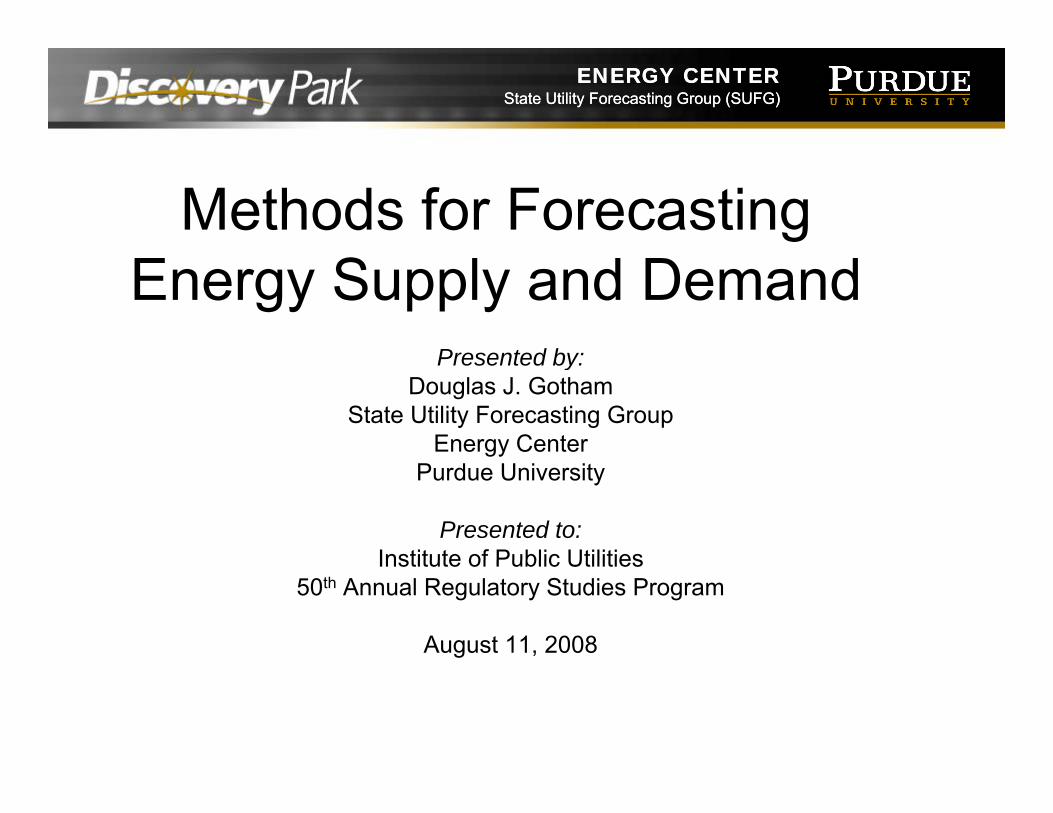
ENERGY CENTER State Utility Forecasting Group (SUFG) ENERGY CENTER State Utility Forecasting Group (SUFG) Methods for Forecasting Energy Supply and Demand Presented by: Presented by: Douglas J. Gotham State Utility Forecasting Group Energy Center Purdue University Presented to: Institute of Public Utilities Institute of Public Utilities 50 th Annual Regulatory Studies Program August 11, 2008
Transcript of Methods for Forecasting Energy Supply and Demand€¦ · ENERGY CENTER State Utility Forecasting...
ENERGY CENTERState Utility Forecasting Group (SUFG)
ENERGY CENTERState Utility Forecasting Group (SUFG)
Methods for Forecasting Energy Supply and Demand
Presented by:Presented by:Douglas J. Gotham
State Utility Forecasting GroupEnergy Center
Purdue University
Presented to:Institute of Public UtilitiesInstitute of Public Utilities
50th Annual Regulatory Studies Program
August 11, 2008
ENERGY CENTERState Utility Forecasting Group (SUFG)
ENERGY CENTERState Utility Forecasting Group (SUFG)
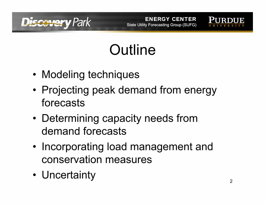
Outline• Modeling techniques• Projecting peak demand from energy• Projecting peak demand from energy
forecastsD t i i it d f• Determining capacity needs from demand forecasts
• Incorporating load management and conservation measures
• Uncertainty2

ENERGY CENTERState Utility Forecasting Group (SUFG)
ENERGY CENTERState Utility Forecasting Group (SUFG)
Using the Past to Predict the Future• What is the next number in the following
sequences?– 0, 2, 4, 6, 8, 10, 12, 14 ….– 0, 1, 4, 9, 16, 25, 36, 49, ...., , , , , , , ,– 0, 1, 3, 6, 10, 15, 21, 28, ....– 0, 1, 2, 3, 5, 7, 11, 13, ....0, , , 3, 5, , , 3,– 0, 1, 1, 2, 3, 5, 8, 13, ....– 8 5 4 9 1 7 68, 5, 4, 9, 1, 7, 6, ….
3

ENERGY CENTERState Utility Forecasting Group (SUFG)
ENERGY CENTERState Utility Forecasting Group (SUFG)
A Simple Example1000
106010801100
1000
1010
1020
100010201040
1020
1030
1040
920940960980
1040
1050
?
900920
1 2 3 4 5 6?
?
4
ENERGY CENTERState Utility Forecasting Group (SUFG)
ENERGY CENTERState Utility Forecasting Group (SUFG)
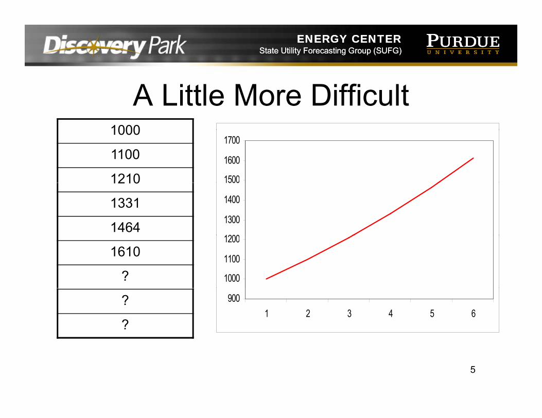
A Little More Difficult10001000
1100
1210 1500
1600
1700
1210
1331
14641200
1300
1400
1500
1610
? 1000
1100
1200
?
?
9001 2 3 4 5 6
5
ENERGY CENTERState Utility Forecasting Group (SUFG)
ENERGY CENTERState Utility Forecasting Group (SUFG)
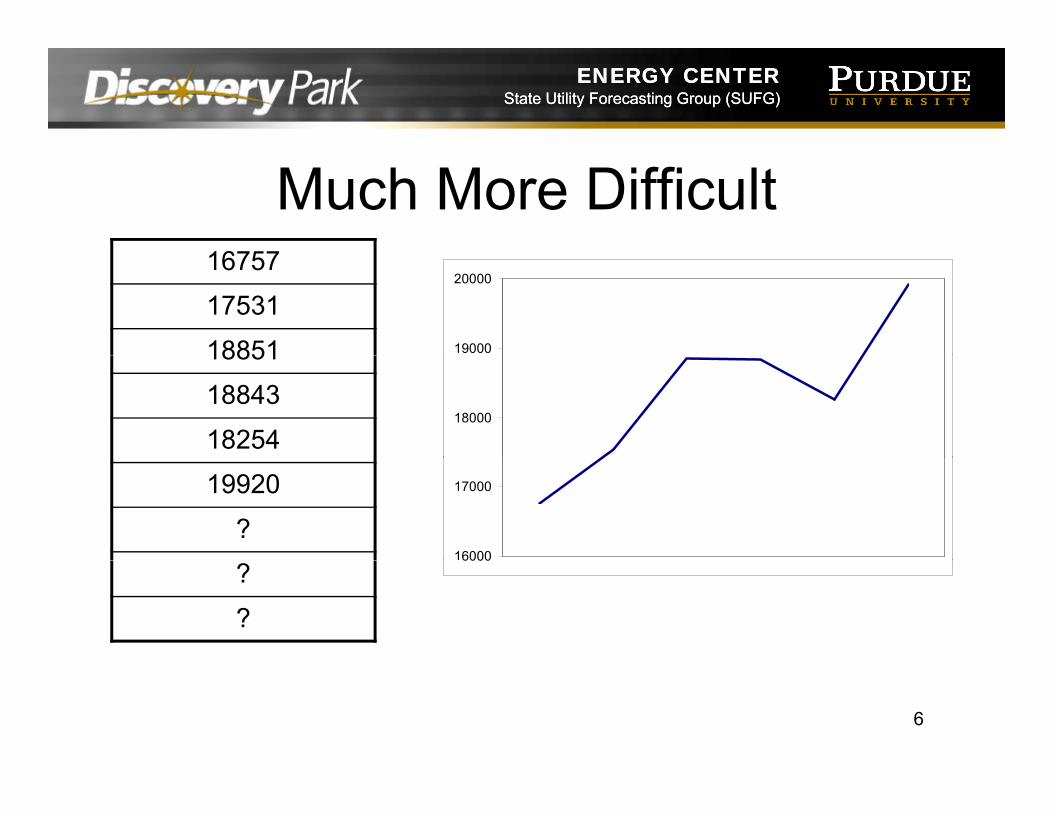
Much More Difficult1675716757
17531
18851 19000
20000
18851
18843
1825418000
19920
?16000
17000
?
?
6000
6

ENERGY CENTERState Utility Forecasting Group (SUFG)
ENERGY CENTERState Utility Forecasting Group (SUFG)
Much More Difficult• The numbers on the previous slide were
the summer peak demands for Indiana f 2000 t 2005from 2000 to 2005.
• They are affected by a number of f tfactors– Weather
E i ti it– Economic activity– Price
Interruptible customers called upon– Interruptible customers called upon– Price of competing fuels 7

ENERGY CENTERState Utility Forecasting Group (SUFG)
ENERGY CENTERState Utility Forecasting Group (SUFG)
Question• How do we find
a pattern in 20000
25000
pthese peak demand
b t10000
15000
numbers to predict the future?
0
5000
1980
1982
1984
1986
1988
1990
1992
1994
1996
1998
2000
2002
2004future?
8

ENERGY CENTERState Utility Forecasting Group (SUFG)
ENERGY CENTERState Utility Forecasting Group (SUFG)
The Short Answer
9

ENERGY CENTERState Utility Forecasting Group (SUFG)
ENERGY CENTERState Utility Forecasting Group (SUFG)
Methods of Forecasting• Time Series
– trend analysis– trend analysis• Econometric
t t l l i– structural analysis• End Use
– engineering analysis
10

ENERGY CENTERState Utility Forecasting Group (SUFG)
ENERGY CENTERState Utility Forecasting Group (SUFG)
Time Series ForecastingLi T d• Linear Trend – Fit the best straight line to the historical data and
assume that the future will follow that line k f tl i th 1st l• works perfectly in the 1st example
– Many methods exist for finding the best fitting line; the most common is the least squares method
• Polynomial Trend• Polynomial Trend– Fit the polynomial curve to the historical data and
assume that the future will follow that line– Can be done to any order of polynomial (square cube– Can be done to any order of polynomial (square, cube,
etc.) but higher orders are usually needlessly complex• Logarithmic Trend
– Fit an exponential curve to the historical data andFit an exponential curve to the historical data and assume that the future will follow that line
• works perfectly for the 2nd example 11

ENERGY CENTERState Utility Forecasting Group (SUFG)
ENERGY CENTERState Utility Forecasting Group (SUFG)
Good News and Bad News• The statistical functions in most commercial
spreadsheet software packages will calculate p p gmany of these for you.
• These may not work well when there is a lot of variability in the historical data.
• If the time series curve does not perfectly fit the historical data, there is model error. – There is normally model error when trying to
forecast a complex systemforecast a complex system.12
ENERGY CENTERState Utility Forecasting Group (SUFG)
ENERGY CENTERState Utility Forecasting Group (SUFG)
M th d U d t A t fMethods Used to Account for Variabilityy
• Modeling seasonality/cyclicalityS thi t h i• Smoothing techniques– Moving averages– Weighted moving averages– Exponentially weighted moving averages
• Filtering techniques• Box-Jenkins
13

ENERGY CENTERState Utility Forecasting Group (SUFG)
ENERGY CENTERState Utility Forecasting Group (SUFG)
Econometric Forecasting• Econometric models attempt to quantify the
relationship between the parameter of interest (output variable) and a number ofinterest (output variable) and a number of factors that affect the output variable.
• ExampleExample– Output variable– Explanatory variable
• Economic activity• Economic activity• Weather (HDD/CDD)• Electricity price• Natural gas priceNatural gas price• Fuel oil price
14

ENERGY CENTERState Utility Forecasting Group (SUFG)
ENERGY CENTERState Utility Forecasting Group (SUFG)
Estimating Relationships• Each explanatory variable affects the output
variable in different ways. The relationships b l l t d i f th th dcan be calculated via any of the methods
used in time series forecasting.– Can be linear polynomial logarithmic movingCan be linear, polynomial, logarithmic, moving
averages, …• Relationships are determined simultaneously
t fi d ll b t fitto find overall best fit.• Relationships are commonly known as
sensitivitiessensitivities.15

ENERGY CENTERState Utility Forecasting Group (SUFG)
ENERGY CENTERState Utility Forecasting Group (SUFG)
Example Sensitivities for State of Mississippiof Mississippi
A 10 percent increase in:
Results in this increasein electricity sales
Electricity price -3 0 percentElectricity price -3.0 percentCooling degree days +0.7 percentReal personal income +7.8 percentReal personal income 7.8 percent
16

ENERGY CENTERState Utility Forecasting Group (SUFG)
ENERGY CENTERState Utility Forecasting Group (SUFG)
End Use Forecasting• End use forecasting looks at individual
devices, aka end uses (e.g., refrigerators)( g g )• How many refrigerators are out there?• How much electricity does a refrigerator use?y g• How will the number of refrigerators change
in the future?• How will the amount of use per refrigerator
change in the future?• Repeat for other end uses
17

ENERGY CENTERState Utility Forecasting Group (SUFG)
ENERGY CENTERState Utility Forecasting Group (SUFG)
The Good News• Account for changes in efficiency levels (new
refrigerators tend to be more efficient than ld ) b th f d folder ones) both for new uses and for
replacement of old equipment• Allow for impact of competing fuels (natural• Allow for impact of competing fuels (natural
gas vs. electricity for heating) or for competing technologies (electric resistance heating vs. heat pump)
• Incorporate and evaluate the impact of demand side management/conservationdemand-side management/conservation programs 18
ENERGY CENTERState Utility Forecasting Group (SUFG)
ENERGY CENTERState Utility Forecasting Group (SUFG)
The Bad News• Tremendously data intensive• Primarily limited to forecasting energy• Primarily limited to forecasting energy
usage, unlike other forecasting methodsMost long term planning electricity– Most long-term planning electricity forecasting models forecast energy and then derive peak demand from the energythen derive peak demand from the energy forecast
19
ENERGY CENTERState Utility Forecasting Group (SUFG)
ENERGY CENTERState Utility Forecasting Group (SUFG)
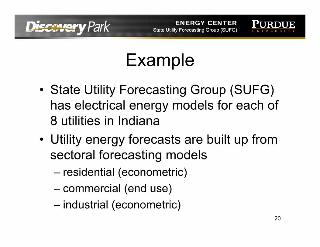
Example• State Utility Forecasting Group (SUFG)
has electrical energy models for each ofhas electrical energy models for each of 8 utilities in Indiana
• Utility energy forecasts are built up from• Utility energy forecasts are built up from sectoral forecasting models
residential (econometric)– residential (econometric)– commercial (end use)
i d t i l ( t i )– industrial (econometric)20

ENERGY CENTERState Utility Forecasting Group (SUFG)
ENERGY CENTERState Utility Forecasting Group (SUFG)
Another Example• The Energy Information Administration’s
National Energy Modeling System (NEMS) gy g y ( )projects energy and fuel prices for 9 census regions
• Energy demand– residential– commercial– industrial
transportation– transportation21

ENERGY CENTERState Utility Forecasting Group (SUFG)
ENERGY CENTERState Utility Forecasting Group (SUFG)
SUFG R id ti l S t M d lSUFG Residential Sector Model• Residential sector
Annual Use per Electric Space Heating Customer
split according to space heating source
500010000150002000025000
– electric– non-electric
M j f t d i
0
Year
1967
1971
1975
1979
1983
1987
1991
1995
1999
2003
Ye a r s
• Major forecast drivers– demographics
households
Annual Use per Non-Electric Space Heating Customer
1000012000
– households– household income– energy prices 0
2000400060008000
10000
7 5 9 3 7 5 9 3energy prices
Year
1967
1971
1975
1979
1983
1987
1991
1995
1999
2003
Ye a r s
22

ENERGY CENTERState Utility Forecasting Group (SUFG)
ENERGY CENTERState Utility Forecasting Group (SUFG)
Residential Model Sensitivities
10 Percent Increase InCauses This Percent
Change in Electric Use
Number of Customers 11.1Electric Rates -2.4Electric Rates 2.4Natural Gas Price 1.0Distillate Oil Prices 0.0Appliance Price -1.8Household Income 2.0
Source: SUFG 2007 Forecast 23
ENERGY CENTERState Utility Forecasting Group (SUFG)
ENERGY CENTERState Utility Forecasting Group (SUFG)
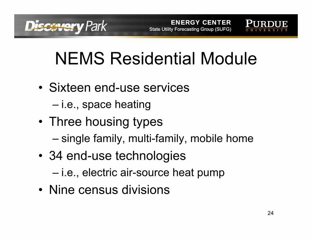
NEMS Residential Module• Sixteen end-use services
– i e space heating– i.e., space heating• Three housing types
i l f il lti f il bil h– single family, multi-family, mobile home• 34 end-use technologies
– i.e., electric air-source heat pump• Nine census divisions
24

ENERGY CENTERState Utility Forecasting Group (SUFG)
ENERGY CENTERState Utility Forecasting Group (SUFG)
SUFG Commercial Sector Model
• Major forecast drivers– floor space inventory
• 14 end uses per building type
space heating air– end use intensity– employment growth– energy prices
– space heating, air conditioning, ventilation, water heating, cooking, refrigeration, lighting, gy p
• 10 building types modeled
ffi t t
mainframe computers, mini-computers, personal computers, office equipment outdoor– offices, restaurants,
retail, groceries, warehouses, schools, colleges health care
equipment, outdoor lighting, elevators and escalators, other
colleges, health care, hotel/motel, miscellaneous 25

ENERGY CENTERState Utility Forecasting Group (SUFG)
ENERGY CENTERState Utility Forecasting Group (SUFG)
Commercial Model Sensitivities
10 Percent Increase InCauses This Percent Change in Electric Use
Electric Rates -2.5N t l G P i 0 2Natural Gas Price 0.2Distillate Oil Prices 0.0Coal Prices 0.0Coal Prices 0.0Electric Energy-weighted Floor Space 12.0
Source: SUFG 2005 Forecast 26

ENERGY CENTERState Utility Forecasting Group (SUFG)
ENERGY CENTERState Utility Forecasting Group (SUFG)
NEMS Commercial Module• Ten end-use services
– i.e., cooking• Eleven building types
– i.e., food service64 d t h l i• 64 end-use technologies– i.e., natural gas range
• Ten distributed generation technologies• Ten distributed generation technologies– i.e., photovoltaic solar systems
• Nine census divisionsNine census divisions27
ENERGY CENTERState Utility Forecasting Group (SUFG)
ENERGY CENTERState Utility Forecasting Group (SUFG)
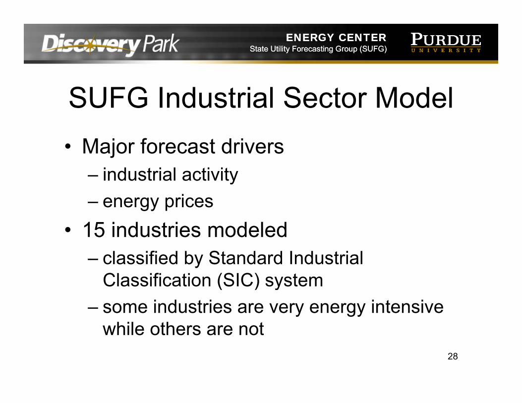
SUFG Industrial Sector Model• Major forecast drivers
– industrial activity– industrial activity– energy prices
• 15 industries modeled• 15 industries modeled– classified by Standard Industrial
Classification (SIC) systemClassification (SIC) system– some industries are very energy intensive
while others are notwhile others are not28

ENERGY CENTERState Utility Forecasting Group (SUFG)
ENERGY CENTERState Utility Forecasting Group (SUFG)
Indiana’s Industrial SectorCurrent Forecast Forecast Forecast
SIC Name
Current Share of
GSP
Current Share of
Electricity Use
Growth in GSP
Originating by Sector
Growth in Electricity by Intensity by
Sector
Forecast Growth in Electricity
Use by Sector
20 F d & Ki d d P d t 3 51 5 61 0 96 0 79 0 1720 Food & Kindred Products 3.51 5.61 0.96 -0.79 0.1724 Lumber & Wood Products 1.95 0.70 0.96 -0.42 0.5425 Furniture & Fixtures 1.60 0.46 0.62 -0.64 -0.0226 Paper & Allied Products 1.36 2.96 0.96 -0.56 0.4027 Printing & Publishing 2.55 1.30 0.96 -0.96 0.0028 Chemicals & Allied Prod cts 14 25 17 10 3 49 0 80 2 7028 Chemicals & Allied Products 14.25 17.10 3.49 -0.80 2.7030 Rubber & Misc. Plastic Products 4.77 6.25 4.52 -0.67 3.8532 Stone, Clay, & Glass Products 1.76 5.30 0.96 -0.67 0.2933 Primary Metal Products 8.55 31.34 1.02 1.76 2.7734 Fabricated Metal Products 6.25 5.29 2.51 -0.76 1.75
35 Industrial Machinery & Equipment 6.73 4.44 1.05 -0.68 0.3736 Electronic & Electric Equipment 16.19 5.54 5.33 -0.56 4.7737 Transportation Equipment 22.89 9.38 3.87 -0.68 3.1938 Instruments And Related Products 4.98 0.77 5.33 -0.86 4.4739 Miscellaneous Manufacturing 1.63 1.06 4.19 -5.24 -1.05
Source: SUFG 2007 Forecast
g
Total Manufacturing 100.00 100.00 3.48 -0.81 2.6729
ENERGY CENTERState Utility Forecasting Group (SUFG)
ENERGY CENTERState Utility Forecasting Group (SUFG)
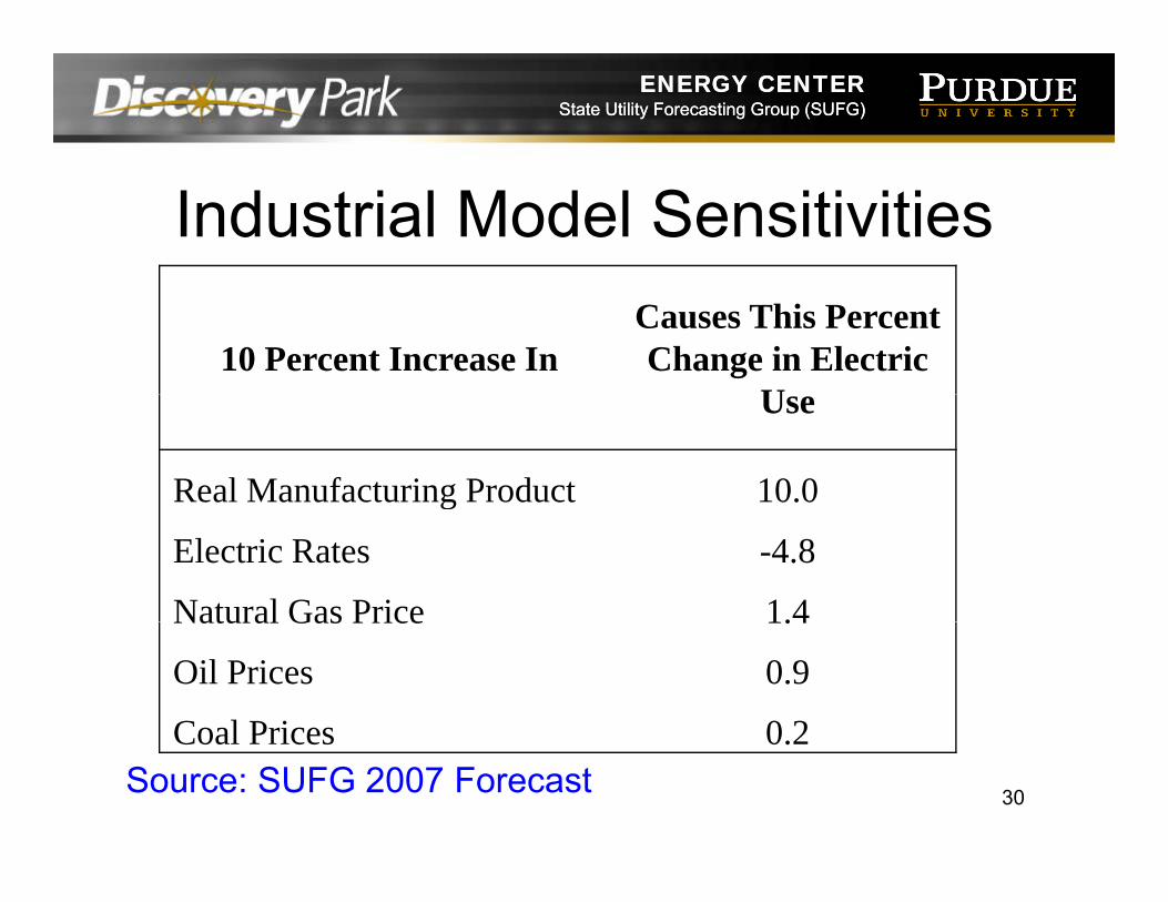
Industrial Model Sensitivities
10 Percent Increase InCauses This Percent Change in Electric
UUse
Real Manufacturing Product 10.0g
Electric Rates -4.8
Natural Gas Price 1.4Natural Gas Price 1.4
Oil Prices 0.9
Coal Prices 0 2Source: SUFG 2007 Forecast
Coal Prices 0.2
30

ENERGY CENTERState Utility Forecasting Group (SUFG)
ENERGY CENTERState Utility Forecasting Group (SUFG)
NEMS Industrial Module• Seven energy-intensive industries
– i e bulk chemicals– i.e., bulk chemicals• Eight non-energy-intensive industries
i t ti– i.e., construction• Cogeneration• Four census regions, shared to nine
census divisions
31

ENERGY CENTERState Utility Forecasting Group (SUFG)
ENERGY CENTERState Utility Forecasting Group (SUFG)
Energy → Peak Demand• Constant load factor / load shape
– Peak demand and energy grow at same rategy g• Constant load factor / load shape for each
sector– Calculate sectoral contribution to peak demand
and sumIf l l d f t ( id ti l) f t t k– If low load factor (residential) grows fastest, peak demand grows faster than energy
– If high load factor (industrial) grows fastest, peakIf high load factor (industrial) grows fastest, peak demand grows slower than energy
32

ENERGY CENTERState Utility Forecasting Group (SUFG)
ENERGY CENTERState Utility Forecasting Group (SUFG)
Energy → Peak Demand• Day types
– Break overall load shapes into typical day– Break overall load shapes into typical day types
• low, medium, high, , g• weekday, weekend, peak day
– Adjust day type for load management and j y yp gconservation programs
– Can be done on a total system level or a sectoral level
33

ENERGY CENTERState Utility Forecasting Group (SUFG)
ENERGY CENTERState Utility Forecasting Group (SUFG)
Load Diversity• Each utility does not see its peak demand at
the same time as the others
• 2005 peak demands occurred at:– Hoosier Energy – 7/25, 6PM
I di Mi hi 8/3 2PM– Indiana Michigan - 8/3, 2PM– Indiana Municipal Power Agency – 7/25, 3PM– Indianapolis Power & Light - 7/25, 3PM– NIPSCO – 6/24, 1PM– PSI Energy – 7/25, 4PM– SIGECO – 7/25 4PMSIGECO 7/25, 4PM– Wabash Valley – 7/24, 5PM
34

ENERGY CENTERState Utility Forecasting Group (SUFG)
ENERGY CENTERState Utility Forecasting Group (SUFG)
Load DiversityTh h id k d d i l h• Thus, the statewide peak demand is less than the sum of the individual peaks
• Actual statewide peak demand can beActual statewide peak demand can be calculated by summing up the load levels of all utilities for each hour of the yearDiversity factor is an indication of the level of• Diversity factor is an indication of the level of load diversity
• Historically, Indiana’s diversity factor has y, ybeen about 96 – 97 percent– that is, statewide peak demand is usually about 96
percent of the sum of the individual utility peak p y pdemands
35

ENERGY CENTERState Utility Forecasting Group (SUFG)
ENERGY CENTERState Utility Forecasting Group (SUFG)
Peak Demand → Capacity Needs• Target reserve margin• Loss of load probability (LOLP)p y ( )• Expected unserved energy (EUE)• Assigning capacity needs to type• Assigning capacity needs to type
– peakingb l d– baseload
– intermediate• Optimization
36

ENERGY CENTERState Utility Forecasting Group (SUFG)
ENERGY CENTERState Utility Forecasting Group (SUFG)
R M i C itReserve Margin vs. Capacity Marging
100%capacity demandCM xcapacity
−=100%capacity demandRM x
d d−
=capacity
• Both reserve margin (RM) and capacity
demand
Both reserve margin (RM) and capacity margin (CM) are the same when expressed in megawatts
diff b il bl i d– difference between available capacity and demand
• Normally expressed as percentagesNormally expressed as percentages37

ENERGY CENTERState Utility Forecasting Group (SUFG)
ENERGY CENTERState Utility Forecasting Group (SUFG)
Reserve Margins• Reserve/capacity margins are relatively
easy to use and understand, but the b t i l tnumbers are easy to manipulate
– Contractual off-system sale can be treated as a reduction in capacity or increase inas a reduction in capacity or increase in demand
• does not change the MW margin, but will g gchange the percentage
– Similarly, interruptible loads and direct load control is sometimes shown as an increasecontrol is sometimes shown as an increase in capacity 38

ENERGY CENTERState Utility Forecasting Group (SUFG)
ENERGY CENTERState Utility Forecasting Group (SUFG)
LOLP and EUEP b bili ti th d th t t f th li bilit• Probabilistic methods that account for the reliability of the various sources of supply
• Loss of load probabilityLoss of load probability– given an expected demand for electricity and a given set
of supply resources with assumed outage rates, what is the likelihood that the supply will not be able to meet thethe likelihood that the supply will not be able to meet the demand?
• Expected unserved energysimilar calculation to find the expected amount of energy– similar calculation to find the expected amount of energy that would go unmet
• Both are used in resource planning to ensure that sufficient capacity is available for LOLP and/or EUE to be less than a minimum allowable level 39

ENERGY CENTERState Utility Forecasting Group (SUFG)
ENERGY CENTERState Utility Forecasting Group (SUFG)
Capacity TypesO th t f it d d i• Once the amount of capacity needed in a given year is determined, the next step is to determine what type of capacity isto determine what type of capacity is needed– peaking (high operating cost, low capital cost)p g ( g p g , p )– baseload (low operating cost, high capital
cost)i t di t li ( ti d it l– intermediate or cycling (operating and capital costs between peaking and baseload)
• some planners only use peaking and baseloadp y p g
40

ENERGY CENTERState Utility Forecasting Group (SUFG)
ENERGY CENTERState Utility Forecasting Group (SUFG)
Assigning Demand to TypeSUFG hi t i l l d h l i f• SUFG uses historical load shape analysis for each of the utilities to assign a percentage of their peak demand to each load typetheir peak demand to each load type
• Percentages vary from utility to utility according to the characteristics of their customers– utilities with a large industrial base tend to have a
higher percentage of baseload demandhigher percentage of baseload demand– those with a large residential base tend to have a
higher percentage of peaking demandR h b kd• Rough breakdown:– baseload 65%, intermediate 15%, peaking 20% 41

ENERGY CENTERState Utility Forecasting Group (SUFG)
ENERGY CENTERState Utility Forecasting Group (SUFG)
Assigning Existing Resources• SUFG then assigns existing generation to
the three types according to age, size, fuel type, and historical usage patterns
• Purchased power contracts are assigned to type according to time period (annual or summer only) and capacity factor
• Power sales contracts are also assigned to type
42

ENERGY CENTERState Utility Forecasting Group (SUFG)
ENERGY CENTERState Utility Forecasting Group (SUFG)
Assigning Capacity Needs to Type• Future resource needs by type are
determined by comparing existing capacity to projected demand while accounting forto projected demand, while accounting for interruptible and buy through loads, as well as firm purchases and sales andas firm purchases and sales and retirement of existing units
• Breakdown of demand by type is not y ypprojected to change across the forecast horizon
43
ENERGY CENTERState Utility Forecasting Group (SUFG)
ENERGY CENTERState Utility Forecasting Group (SUFG)
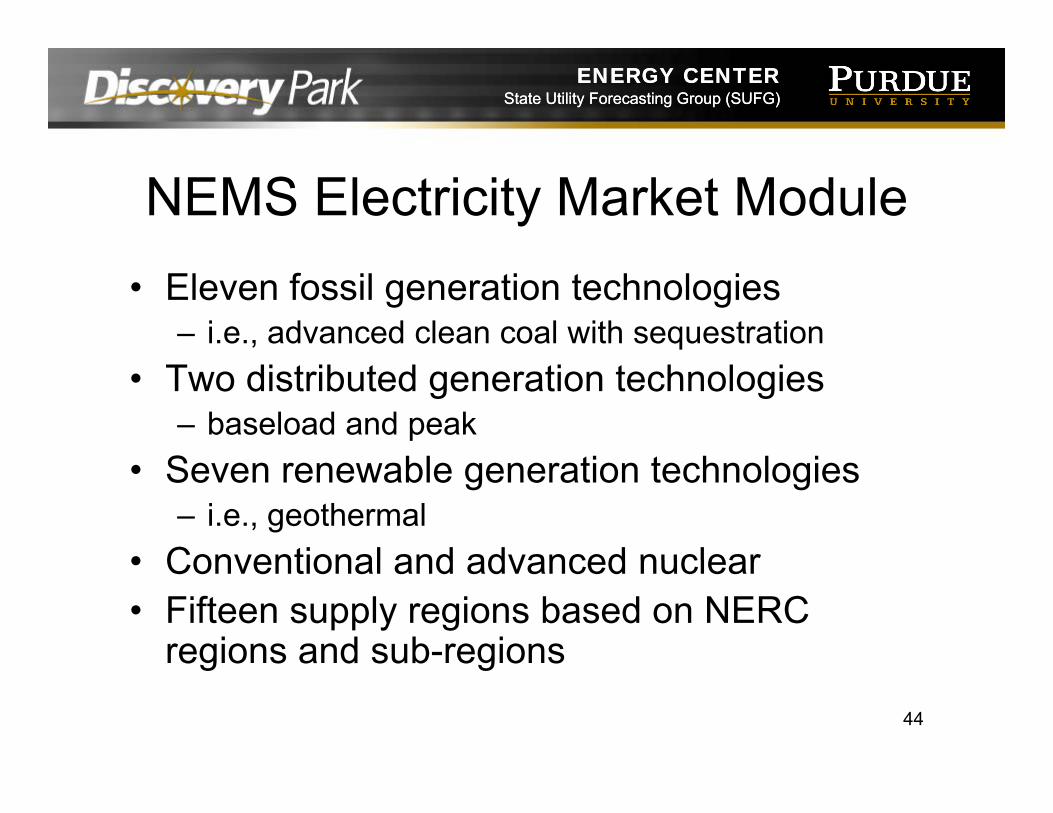
NEMS Electricity Market Module• Eleven fossil generation technologies
– i.e., advanced clean coal with sequestration• Two distributed generation technologies
– baseload and peakS bl ti t h l i• Seven renewable generation technologies– i.e., geothermal
• Conventional and advanced nuclear• Conventional and advanced nuclear• Fifteen supply regions based on NERC
regions and sub-regionseg o s a d sub eg o s
44

ENERGY CENTERState Utility Forecasting Group (SUFG)
ENERGY CENTERState Utility Forecasting Group (SUFG)
Load Management andLoad Management and Conservation Measures
• Direct load control and interruptible loads generally affect peak demand but not energy forecasts– delay consumption from peak time to off-peak time
ll bt t f k d d j ti– usually subtract from peak demand projections• Efficiency and conservation programs generally
affect both peak demand and energy forecastsaffect both peak demand and energy forecasts– consumption is reduced instead of delayed– usually subtract from energy forecast before peakusually subtract from energy forecast before peak
demand calculations45

ENERGY CENTERState Utility Forecasting Group (SUFG)
ENERGY CENTERState Utility Forecasting Group (SUFG)
Sources of Uncertainty• Exogenous assumptions
– forecast is driven by a number of assumptions y p(e.g., economic activity) about the future
• Stochastic model error– it is usually impossible to perfectly estimate the
relationship between all possible factors and the outputoutput
• Non-stochastic model error– bad input data (measurement/estimation error)bad input data (measurement/estimation error)
46

ENERGY CENTERState Utility Forecasting Group (SUFG)
ENERGY CENTERState Utility Forecasting Group (SUFG)
Alternate ScenariosGi th t i t• Given the uncertainty surrounding long-term forecasts, it is 200000
250000 History
High
Forecast
,inadvisable to follow one single forecast
100000
150000
GW
h
Base
Low
• SUFG develops alternative scenarios 0
50000
80 83 86 89 92 95 98 01 04 07 0 3 6 9 22 25
by varying the input assumptions
198
198
198
198
199
199
199
200
200
200
201
201
201
201
202
202
Year
Source: SUFG 2007 Forecast 47

ENERGY CENTERState Utility Forecasting Group (SUFG)
ENERGY CENTERState Utility Forecasting Group (SUFG)
Back to the Short Answer
48

ENERGY CENTERState Utility Forecasting Group (SUFG)
ENERGY CENTERState Utility Forecasting Group (SUFG)
Further Information• State Utility Forecasting Group
– http://www purdue edu/dp/energy/SUFG/– http://www.purdue.edu/dp/energy/SUFG/• Energy Information Administration
htt // i d /i d ht l– http://www.eia.doe.gov/index.html
49