MESSENGER: Exploring Mercury’s...

Space Sci RevDOI 10.1007/s11214-007-9154-x

MESSENGER: Exploring Mercury’s Magnetosphere

James A. Slavin · Stamatios M. Krimigis · Mario H. Acuña · Brian J. Anderson ·Daniel N. Baker · Patrick L. Koehn · Haje Korth · Stefano Livi · Barry H. Mauk ·Sean C. Solomon · Thomas H. Zurbuchen

Received: 22 May 2006 / Accepted: 1 February 2007© Springer Science+Business Media, Inc. 2007

Abstract The MErcury Surface, Space ENvironment, GEochemistry, and Ranging (MES-SENGER) mission to Mercury offers our first opportunity to explore this planet’s miniaturemagnetosphere since the brief flybys of Mariner 10. Mercury’s magnetosphere is unique inmany respects. The magnetosphere of Mercury is among the smallest in the solar system;its magnetic field typically stands off the solar wind only ∼1000 to 2000 km above the sur-face. For this reason there are no closed drift paths for energetic particles and, hence, noradiation belts. Magnetic reconnection at the dayside magnetopause may erode the subsolarmagnetosphere, allowing solar wind ions to impact directly the regolith. Inductive currentsin Mercury’s interior may act to modify the solar wind interaction by resisting changes

J.A. Slavin (�)Heliophysics Science Division, Goddard Space Flight Center, Code 670, Greenbelt, MD 20771,USAe-mail: [email protected]

S.M. Krimigis · B.J. Anderson · H. Korth · S. Livi · B.H. MaukThe Johns Hopkins University Applied Physics Laboratory, Laurel, MD 20723, USA

M.H. AcuñaSolar System Exploration Division, Goddard Space Flight Center, Code 690, Greenbelt, MD20771, USA

D.N. BakerLaboratory for Atmospheric and Space Physics, University of Colorado, Boulder, CO 80303, USA

P.L. KoehnPhysics and Astronomy Department, Eastern Michigan University, Ypsilanti, MI 48197, USA

S.C. SolomonDepartment of Terrestrial Magnetism, Carnegie Institution of Washington, Washington, DC 20015,USA

T.H. ZurbuchenDepartment of Atmospheric, Oceanic and Space Sciences, University of Michigan, Ann Arbor,MI 48109, USA

J.A. Slavin et al.

due to solar wind pressure variations. Indeed, observations of these induction effects maybe an important source of information on the state of Mercury’s interior. In addition, Mer-cury’s magnetosphere is the only one with its defining magnetic flux tubes rooted beneaththe solid surface as opposed to an atmosphere with a conductive ionospheric layer. Thislack of an ionosphere is probably the underlying reason for the brevity of the very intense,but short-lived, ∼1–2 min, substorm-like energetic particle events observed by Mariner 10during its first traversal of Mercury’s magnetic tail. Because of Mercury’s proximity to thesun, 0.3–0.5 AU, this magnetosphere experiences the most extreme driving forces in thesolar system. All of these factors are expected to produce complicated interactions involv-ing the exchange and recycling of neutrals and ions among the solar wind, magnetosphere,and regolith. The electrodynamics of Mercury’s magnetosphere are expected to be equallycomplex, with strong forcing by the solar wind, magnetic reconnection, and pick-up of plan-etary ions all playing roles in the generation of field-aligned electric currents. However,these field-aligned currents do not close in an ionosphere, but in some other manner. Inaddition to the insights into magnetospheric physics offered by study of the solar wind–Mercury system, quantitative specification of the “external” magnetic field generated bymagnetospheric currents is necessary for accurate determination of the strength and multi-polar decomposition of Mercury’s intrinsic magnetic field. MESSENGER’s highly capableinstrumentation and broad orbital coverage will greatly advance our understanding of boththe origin of Mercury’s magnetic field and the acceleration of charged particles in smallmagnetospheres. In this article, we review what is known about Mercury’s magnetosphereand describe the MESSENGER science team’s strategy for obtaining answers to the out-standing science questions surrounding the interaction of the solar wind with Mercury andits small, but dynamic, magnetosphere.

Keywords Planetary magnetospheres · Reconnection · Particle acceleration · Substorms ·Mercury · MESSENGER

1 Introduction: What Do We Presently Know and How Do We Know It?

Launched on November 2, 1973, Mariner 10 (M10) executed the first reconnaissance ofMercury during its three encounters on March 29, 1974, September 21, 1974, and March16, 1975 (see reviews by Ness 1979; Russell et al. 1988; Slavin 2004; Milillo et al. 2005).All flybys occurred at a heliocentric distance of 0.46 AU, but only the first (Mercury I) andthird (Mercury III) encounters passed close enough to Mercury to return observations ofthe solar wind interaction and the planetary magnetic field. The first encounter targeted theplanetary “wake” and returned surprising observations that indicate a significant intrinsicmagnetic field. The closest approach to the surface during this passage was 723 km where apeak magnetic field intensity of 98 nT was observed (Ness et al. 1974). During Mercury I themagnetic field investigation observed clear bow shock and magnetopause boundaries alongwith the lobes of the tail and the cross-tail current layer (Ness et al. 1974, 1975, 1976).The Mercury III observations were of great importance because they confirmed that themagnetosphere was indeed produced by the interaction of the solar wind with an intrinsicplanetary magnetic field. Once corrected for the differing closest approach distances, thepolar magnetic fields measured during Mercury III are about twice as large as those alongthe low-latitude Mercury I trajectory, consistent with a primarily dipolar planetary field.Magnetic field models derived using different subsets of the Mariner 10 data and variousassumptions concerning the external magnetospheric magnetic field indicate that the tilt of


the dipole relative to the planetary rotation axis is about 10◦, but the longitude angle of thedipole is very poorly constrained (Ness et al. 1976).

The plasma investigation was hampered by a deployment failure that kept it from re-turning ion measurements. Fortunately, the electron portion of the plasma instrument didoperate as planned (Ogilvie et al. 1974). Good correspondence was found between the mag-netic field and plasma measurements as to the locations of the Mercury I and III bow shockand magnetopause boundaries. Plasma speed and density parameters derived from the elec-tron data produced consistent results regarding bow shock jump conditions and pressurebalance across the magnetopause (Ogilvie et al. 1977; Slavin and Holzer 1979a). WithinMercury’s magnetosphere, plasma density was found to be higher than that observed at Earthby a factor comparable to the ratio of the solar wind density at the orbits of the two planets(Ogilvie et al. 1977). Similar correlations are observed between solar wind and plasma sheetdensity at Earth (Terasawa et al. 1997). Throughout the Mercury I pass plasma sheet-typeelectron distributions were observed with an increase in temperature beginning near closestapproach coincident with a series of intense energetic particle events (Ogilvie et al. 1977;Christon 1987).

Several groups have estimated the magnetic moment of Mercury from the observationsmade during Mercury I and III. Conducting a least-squared fit of the Mercury I data to anoffset tilted dipole, Ness et al. (1974) obtained a dipole moment of 227 nTR3

M , where RM isMercury’s radius (1 RM = 2439 km), and a dipole tilt angle of 10◦ relative to the planetaryrotation axis. Ness et al. (1975) considered a centered dipole and an external contributionto the measured magnetic field and found the strength of the dipole to be 349 nTR3

M fromthe same data set. From the Mercury III encounter observations these authors determined adipole moment of 342 nTR3

M (Ness et al. 1976). Higher-order contributions to the internalmagnetic field were examined by Jackson and Beard (1977) (quadrupole) and Whang (1977)(quadrupole, octupole). Both sets of authors reported 170 nTR3

M as the dipole contributionto Mercury’s intrinsic magnetic field. The cause for the large spread in the reported estimatesof the dipole term is the limited spatial coverage of the observations, which is insufficientfor separating the higher-order multipoles (Connerney and Ness 1988), and variable mag-netic field contributions from the magnetospheric current systems (Slavin and Holzer 1979b;Korth et al. 2004; Grosser et al. 2004).

Mercury’s magnetosphere is one of the most dynamic in the solar system. A glimpse ofthis variability was captured during the Mercury I encounter. Less than a minute after M10entered the plasma sheet during this first flyby there was a sharp increase in the Bz fieldcomponent (Ness et al. 1974). The initial sudden Bz increase and subsequent quasi-periodicincreases are nearly coincident with strong enhancements in the flux of >35 keV electronsobserved by the cosmic ray telescopes (Simpson et al. 1974; Eraker and Simpson 1986;Christon 1987). Taken together, these M10 measurements are very similar to the “dipo-larizations” of the near-tail magnetic field frequently observed in association with en-ergetic particle “injections” at Earth (Christon et al. 1987). This energetic particle sig-nature, and several weaker events observed later in the outbound Mercury I pass, wasinterpreted as strong evidence for substorm activity and, by inference, magnetic recon-nection in the tail (Siscoe et al. 1975; Eraker and Simpson 1986; Baker et al. 1986;Christon 1987).

The stresses exerted on planetary magnetic fields by magnetospheric convection aretransmitted down to the planet and its environs by Alfven waves carrying field-aligned cur-rent (FAC). At planets with electrically conductive ionospheres, such as the Earth, Jupiter,and Saturn, these current systems are well observed and transfer energy to their ionospheres,an important energy sink as well as serving as a “brake” that limits the speed and rate

J.A. Slavin et al.

of change of the plasma convection (Coroniti and Kennel 1973). Mercury’s atmosphere,however, is a tenuous exosphere, and no ionosphere possessing significant electrical con-ductance is present (Lammer and Bauer 1997). For these reasons, the strong variations inthe east-west component of the magnetic field measured by M10 during the Mercury I passseveral minutes following the substorm-like signatures may be quite significant. These per-turbations were first examined by Slavin et al. (1997), who concluded that the spacecraftcrossed three FAC sheets similar to those often observed at the Earth (Iijima and Potemra1978). The path by which these currents close is not known, but their existence may indicatethat the conductivity of the regolith is greater than is usually assumed (e.g., Hill et al. 1976)or other closure paths exist (Glassmeier 2000).

Another unique aspect of Mercury concerns the origin of its very tenuous, collisionless,neutral atmosphere (e.g., Goldstein et al. 1981). Three exospheric neutral species, Na, K,and Ca, have been measured spectroscopically from the Earth (Potter and Morgan 1985,1986; Bida et al. 2000), and three other species, H, He, and O, were observed by Mariner10 (Broadfoot et al. 1976). The large day-to-day variability in the sodium and potassiumexosphere at Mercury, including changes in both total density and global distribution, arequite striking and may be linked to dynamic events in the solar wind and their effect on themagnetosphere. For example, Potter et al. (1999) suggested that the underlying cause of thelarge day-to-day changes in the neutral exosphere might be the modulation of the surfacesputtering rates by variations in the spatial distribution and intensity of solar wind protonimpingement on the surface. Our present understanding of Mercury’s neutral atmosphereand the contributions that the MErcury Surface, Space ENvironment, GEochemistry, andRanging (MESSENGER) mission will make to this discipline are the subject of a companionpaper (Domingue et al. 2007).

2 MESSENGER Science Instruments

The MESSENGER spacecraft, instrument payload, and mission plan have been describedelsewhere (Gold et al. 2001). Here we provide a brief overview to emphasize the natureof the measurements to be returned and how they will be used to achieve the mission’sscientific objectives (Solomon et al. 2001, 2007). The MESSENGER spacecraft is shown inFig. 1. A key aspect of its design is the presence of a large sunshade that faces sunward whenthe spacecraft is closer than 0.9 AU to the Sun. The spacecraft is three-axis stabilized, butrotations about the Sun-spacecraft axis will be carried out while in Mercury orbit to orientsome of the instruments toward the surface.

The MESSENGER Magnetometer (MAG) is described in detail by Anderson et al.(2007). The triaxial sensor is mounted at the end of a 3.6-m boom to minimize the mag-nitude of stray spacecraft-generated magnetic fields at the MAG sensor location. Groundtesting and in-flight calibration have shown that the intensity of uncorrectable (i.e., variable)stray fields will be less than 0.1 nT (Anderson et al. 2007). While the magnetometer is ca-pable of measuring the full strength of the Earth’s field for integration and check-out, it isdesigned to operate in its most sensitive field range of ±1500 nT per axis when the space-craft is orbit about Mercury. The 16-bit telemetered resolution yields a digital resolutionof 0.05 nT. In the baseline mission plan, the sampling rate of the instrument will be variedaccording to a pre-planned schedule from 2 to 20 vectors s−1 once in orbit about Mercury.Additionally, 8-minute intervals of 20-vectors s−1 burst data will be acquired during peri-ods of lower-rate continuous sampling. The accuracy of the MESSENGER magnetic fieldmeasurements is 0.1%.


Fig. 1 The MESSENGER spacecraft behind its sunshade. Note the adapter ring at the bottom of the vehiclewhich encloses the planet-nadir-pointing instruments. The Magnetometer (MAG) is located at the end of a3.6-m double-hinged boom. The FIPS and EPS sensors are shown along with arrows indicating their locationson the spacecraft

The MESSENGER Energetic Particle and Plasma Spectrometer (EPPS) is described indetail by Andrews et al. (2007). EPPS is composed of two charged-particle detector sys-tems, the Fast Imaging Plasma Spectrometer (FIPS) and the Energetic Particle Spectrometer(EPS). FIPS has a near-hemispherical field of view and accepts ions with an energy-to-charge ratio from 0.05 to 20 keV/q. EPS has a 12◦ × 160◦ field of view and accepts ionsand electrons with energies of 10 keV to 5 MeV and 10 keV to 400 keV, respectively. TheEPPS sensors are mounted between the attach points for the MAG boom and one of thesolar arrays. The fields of view of both the FIPS and EPS are such that they will measurecharged particles coming from the anti-sunward direction, as well as from above and be-low the spacecraft. The FIPS field of view also encompasses the sunward direction, but thisportion of its field-of-view is blocked by the spacecraft and the sunshade. The EPPS mea-surements are central to resolving the issues that arose from the incomplete and ambiguousenergetic particle measurements of M10. The energetic particle measurements of Simpsonet al. (1974) were compromised by electron pileup in the proton channel (Armstrong et al.1975). They were later reinterpreted as having been responding to intense fluxes of >35 keVelectrons (Christon 1987).

3 MESSENGER Mission Plan

When evaluating the potential scientific impact of in-situ magnetospheric measurements, thespatial coverage of the critical boundaries and regions is one of the most important factors.

J.A. Slavin et al.

Fig. 2 Orthogonal views of the 12-hr-long MESSENGER orbit. The left-hand image shows the orbital plane;periapsis and apoapsis altitudes are 200 km and 15 193 km, respectively. The 80◦ inclination of the orbit isapparent in the orthogonal view in the right-hand image

Figure 2 shows the highly inclined, eccentric orbit that MESSENGER will achieve followinginsertion and trim maneuvers. This orbit represents a carefully considered trade between thesometimes competing requirements of the planetary interior, surface geology, atmosphericand magnetospheric science investigations and engineering constraints, particularly thoserelated to the thermal environment (Solomon et al. 2001; Santo et al. 2001). This orbitsatisfies the primary requirements of all of these planetary science disciplines and will enablean outstanding set of measurements to be gathered.

From the standpoint of the magnetosphere, the most informative view of the MESSEN-GER orbital coverage is to examine it relative to the bow shock and magnetopause surfaces.These boundaries are, to first order, axially symmetric with respect to the X axis in Mercury-Solar-Orbital (MSO) coordinates. This coordinate system is the Mercury equivalent of thefamiliar Geocentric-Solar-Ecliptic (GSE) system used at the Earth. In this system XMSO isdirected from the planet’s center to the Sun, YMSO is in the plane of Mercury’s orbit and pos-itive opposite to the planetary velocity vector, and ZMSO completes the right handed system.Mercury’s rotation axis is normal to its orbital plane and, therefore, parallel to the ZMSO

axis. As discussed more fully in Anderson et al. (2007), Mercury’s magnetic field is bestdescribed by a planet-centered dipole whose tilt relative to the ZMSO axis is about 10◦ (Con-nerney and Ness 1988). However, the longitude of Mercury’s magnetic poles are not wellconstrained by the Mariner 10 data (Ness et al. 1976). (Note: for many science applicationsthe MSO coordinates will be “aberrated” using the relative speeds of the planet and the solarwind so that the X′

MSO axis is opposite to the mean solar wind velocity direction in the restframe of Mercury. Due to the high orbital speed of Mercury, especially at perihelion, theaberration angle can approach, and for slow solar wind speeds exceed 10°.)

The efficacy of the MESSENGER orbit for magnetospheric investigations may bejudged by plotting these boundaries and the trace of the orbit over a Mercury year in the(Y 2

MSO + Z2MSO)1/2 versus XMSO and ZMSO versus YMSO planes. In Figs. 3a and 3b, bow


Fig. 3a Projection of the firstMercury year of predicted orbitsfor MESSENGER onto theXMSO–(Y 2

MSO + Z2MSO)1/2

plane. The conic traces in red arethe expected mean locations ofthe magnetopause and bow shockboundaries on the basis of thetwo M10 encounters

Fig. 3b Projection of the firstMercury year of predicted orbitsfor MESSENGER onto theYMSO–ZMSO plane. The circulartraces are the expected meanlocations of the magnetopauseand bow shock boundaries in theXMSO = 0 plane on the basis oftwo M10 encounters

shock and magnetopause surfaces are displayed based upon the subsolar magnetopause alti-tudes for northward Bz for a 6 × 10−8 dyne/cm2 solar wind pressure determined by Slavin

J.A. Slavin et al.

and Holzer (1979a). Mariner 10 crossed these boundaries too few times, over too restrictedof a range of solar zenith angles, to allow their shape to be accurately mapped. Hence, ter-restrial bow shock and magnetopause shapes from Slavin and Holzer (1981) and Holzer andSlavin (1978), respectively, have been assumed. As shown, the MESSENGER orbit will pro-vide dense sampling of all of the primary regions of the magnetosphere and its interactionwith the solar wind. The low-altitude polar passes in the northern hemisphere provide anexcellent opportunity to observe and map field aligned currents. The region south of Mer-cury’s orbital plane is better sampled at high altitudes than those to the north. However,we expect that Mercury’s magnetosphere possesses considerable north-south symmetry. Inthis manner, the MESSENGER orbit provides nearly comprehensive coverage of Mercury’smagnetosphere and solar wind boundaries sunward of XMSO ∼ −3 RM .

4 Solar Wind–Magnetosphere Interaction

4.1 What Is the Origin of Mercury’s Magnetic Field?

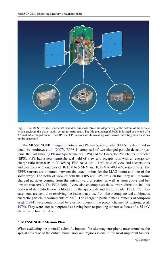
A planet’s spin axis orientation and rotation rate, its atmosphere, the existence and natureof any satellites, and its location within the heliosphere are all important factors influencingmagnetospheric structure and dynamics. However, the single most important factor is thenature of its magnetic field, consisting of the magnetic field intrinsic to the planet and anexternal contribution due to magnetospheric currents. As shown in Fig. 4, the sum of theprimarily dipolar planetary magnetic field and the fields due to the external currents producea magnetospheric magnetic field that is very different from a vacuum dipole even quite closeto the planet’s surface. On the dayside, the magnetic field is greatly compressed; the intensitynear the subsolar point is about twice that due to the planetary field alone. Conversely, thesurface magnetic field around midnight is somewhat reduced from that due to the planetalone, while at higher altitudes on the nightside the local magnetic field is much strongerthan the planetary dipole field would predict due to the current systems that form the longextended magnetotail.

Possible sources for Mercury’s magnetic field are an active dynamo, thermoremanentmagnetization of the crust, or a combination thereof. On the basis of analogy with the Earth,it is often assumed that the source of Mercury’s magnetic field is an active dynamo. Althoughthermal evolution models predict the solidification of a pure iron core early in Mercury’shistory (Solomon 1976), even small quantities of light alloying elements, such as sulfur oroxygen, could have prevented the core from freezing (Stevenson et al. 1983). An activehydrodynamic (Stevenson 1983) or thermoelectric (Stevenson 1987; Giampieri and Balogh2002) dynamo operating at Mercury is, therefore, a strong possibility.

Thermoremanent magnetization of the crust may have been induced either by a largeexternal (i.e., solar or nebular) magnetic field or by an internal dynamo that existed ear-lier in the planet’s history. The former possibility is implausible because any early solar ornebular field would presumably have decayed much faster than the timescale for thicken-ing of Mercury’s lithosphere (Stevenson 1987). The latter hypothesis of an early dynamoas the source for thermoremanent magnetization at Mercury faces additional requirementsset forth by the magnetostatic theorem of Runcorn (1975a, 1975b). Runcorn showed thatthe symmetry of the magnetic field due to thermoremanent magnetization of a uniform, thinshell by a formerly active internal dynamo at the planet’s center does not produce a mag-netic field external to the planet. However, Runcorn’s theorem is valid only under severalideal conditions, including that (1) the permeability of the magnetized shell was uniform


Fig

.4M

ercu

ry’s

mag

netic

field

and

the

stro

ngas

ymm

etri

esin

trod

uced

byits

inte

ract

ion

with

the

sola

rw

ind

(Cop

yrig

htE

urop

ean

Spac

eA

genc

y)

J.A. Slavin et al.

(Stephenson 1976), (2) the cooling of the planetary interior occurred from the outermostlayer progressively inward (Srnka 1976), and (3) the thermal structure of the lithosphereexhibited no asymmetries during the cooling process (Aharonson et al. 2004). Breaking anyof the above stringent conditions could result in a net planetary magnetic moment. Hence,crustal magnetization cannot be excluded as a source for some or all of Mercury’s plane-tary magnetic field. More comprehensive discussions of the important issues surroundingthe origins of Mercury’s magnetic field and the contributions to their solution to be made byMESSENGER can be found in companion papers by Anderson et al. (2007) and Zuber etal. (2007).

4.2 How Will MESSENGER Measurements Be Used to Determine the Origin ofMercury’s Intrinsic Magnetic Field?

Determining the origin of Mercury’s magnetic field is one of MESSENGER’s prime ob-jectives. The approach to addressing this objective will be to produce an accurate repre-sentation, or “map,” of Mercury’s intrinsic magnetic field and use it to distinguish amongthe several hypotheses for the field’s origin. This process, combined with the MESSEN-GER gravity and altimetry investigations, should ultimately yield considerable insight intothe interior structure and evolution of this small planet. Clues to the origin of the planetarymagnetic field are also expected to be found in the multipole decomposition of the planetaryfield, which will be retrieved from an inversion of the magnetic field measurements.

The principal external current systems are the magnetopause current that confines muchof the magnetic flux originating in the planet to the magnetospheric cavity and the cross-tailcurrent layer that separates the two lobes of the tail. A “ring current” due to the drift motionof trapped energetic ions and electrons, observed at Earth during geomagnetic “storms,” isnot expected because of the absence of closed drift paths in Mercury’s magnetosphere. How-ever, a “partial” ring current may exist at times (see Glassmeier 2000). Finally, Slavin et al.(1997) have reported evidence of high-latitude field-aligned currents at Mercury, but owingto the absence of a conducting ionosphere, their global distribution may differ significantlyfrom those at Earth.

Two methods of accounting for the external field contribution are typically used wheninverting the measured magnetic field to create model descriptions of the intrinsic magneticfield. In the first, a spherical harmonic expansion series is derived for the planetary field andthe external field is treated by adding a scalar potential function. Whether a scalar repre-sentation best captures the external contribution is not clear. The second approach appliesour present understanding of magnetospheric current systems to model the individual mag-netospheric current systems and subtract their contribution prior to evaluating the structureof the intrinsic field. Several workers have adapted geometric descriptions of the magneticfields from magnetopause currents and tail currents in the Earth’s magnetosphere to Mer-cury’s magnetosphere (Whang 1977; Korth et al. 2004). Our ability to characterize reliablythe structure of Mercury’s intrinsic magnetic field is, therefore, determined by the extent towhich the external field can be understood and accurately modeled.

The extensive spatial and temporal coverage of the MESSENGER observations willyield a number of important benefits. First, the residuals remaining after fitting for dif-ferent external field conditions will vary more distinctively, thus allowing better deter-mination of the quality of the inversion solutions. Second, cross-correlation among thespherical harmonic coefficients will be significantly reduced, allowing for the deriva-tion of improved quasi-linearly independent higher-order moments of the field repre-sentation (see Connerney and Ness 1988). Simulations of the magnetic field environ-ment at Mercury have shown that the dipole moment should be recoverable to within


10% without applying any corrections for the external field (Giampieri and Balogh 2001;Korth et al. 2004). Further, the magnetic field data will provide significant clues about theoccurrence of dynamic magnetospheric processes, so it will be possible to pre-select the datato be included in the inversion and reduce dynamic effects to a minimum. It is expected thatthe most reliable solutions will be afforded by the most carefully chosen “northward IMF—non-substorm” observations when the magnetospheric currents are weakest. We expect thatthe ultimate accuracy will be determined by a trade-off between statistical uncertainty, whichgrows as the number of observations is reduced, and systematic error, which decreases asthe data are more carefully selected. In any case, the ultimately achievable accuracy for thedipole term will be fairly high, on the order of a few percent, and many higher-order termsshould also be reliably recovered.

Additional analyses will examine the fine structure of Mercury’s crustal magnetic field.The altitudes of the MESSENGER orbit in the northern hemisphere are sufficiently low(200-km minimum altitude) that field structures due to crustal anomalies, if present, can bedirectly mapped. The closest approach points of the three flybys are also at 200 km altitudebut at low latitudes. Large crustal remanent fields were found at Mars (Acuña et al. 1998,1999) and may also be present at Mercury, although the carriers of the remanence and theinternal field history are probably very different for the two bodies. If only those magneticfeatures having a lateral extent larger than the spacecraft altitude can be resolved, then theeffective longitudinal and latitudinal resolution is determined by the spacecraft orbit. Ac-cordingly, we expect to be able to resolve magnetic features with horizontal dimensions of5◦(about 200 km) near the orbit-phase periapsis at ∼60–70◦ N latitude and near the closestapproach points of the flybys.

In summary, the MESSENGER data can be used to discriminate between the varioushypotheses for Mercury’s magnetic field only to the extent that the competing theories makediffering predictions involving quantities that can be measured directly or inferred from thedata. Unfortunately, the knowledge regarding the interior of Mercury is so limited that itis difficult to forecast now how specific hypotheses will be validated or ruled out simplythrough the generation of a more complete and accurate mapping of the planetary magneticfield. The more likely scenario is that all of MESSENGER’s measurements taken togetherwill reveal unexpected features of the planet, its interior, and magnetic field that cannot beaccommodated by the present hypotheses for the origin of its intrinsic magnetic field – thus,allowing some or most to be discarded and replaced by new theories and models.

4.3 How, When, and Where Does the Solar Wind Impact the Planet?

The manner, flux, energy spectrum, and location of solar wind and solar energetic particle(SEP) impact upon the surface is important because of the role that these processes play insputtering neutrals out of the regolith into the exosphere and their contribution to changingthe appearance and physical properties of the surface (Killen et al. 1999, 2001; Lammer etal. 2003; Sasaki and Kurahashi 2004). Solar wind and SEP charged particles may interceptthe surface by two mechanisms. First, finite gyroradius effects can result in ions being lostto collisions with regolith material wherever the strength of the magnetospheric magneticfield and the height of the magnetopause is such that their centers of gyration are withinone Larmor radius of the surface (Siscoe and Christopher 1975; Slavin and Holzer 1979a).Second, “open” magnetospheric flux tubes with one end rooted in the planet and the otherconnected to the upstream interplanetary magnetic field will act as a “channel” that guidescharged particles down to the surface, except for those that “mirror” prior to impact (Kabinet al. 2000; Sarantos et al. 2001; Massetti et al. 2003).

J.A. Slavin et al.

Fig. 5 Schematic view of themagnetosphere of Mercury.Regions with low plasmatemperature (solar wind and taillobes) are colored blue while thehotter regions (innermagnetosphere and plasma sheet)are shown in redder hues. Thetwo images illustrate the extremecases of minimal (A) andmaximal (B) tail flux expectedfor strongly northward andsouthward interplanetarymagnetic field, respectively

An idealized view of Mercury’s magnetosphere under a northward interplanetary mag-netic field (IMF), based on the Mariner 10 measurements, is presented in Fig. 5(a). It hasbeen drawn using an image of the Earth’s magnetosphere and increasing the size of theplanet by a factor of ∼7–8 to compensate for the relative weakness of the dipole fieldand the high solar wind pressure at Mercury (Ogilvie et al. 1977). The mean ∼1.5 RM

distance from the center of Mercury to the nose of the magnetosphere inferred from theMariner 10 measurements (Siscoe and Christopher 1975; Ness et al. 1976; Russell 1977;Slavin and Holzer 1979a) corresponds to 10–11 RE , where RE is Earth’s radius and1 RE = 6378 km.

Whether or not the solar wind is ever able to compress the dayside magnetosphere to thepoint where solar wind ions directly impact the surface at low latitudes remains a topic ofconsiderable interest and controversy. Siscoe and Christopher (1975) were the first to takea long time series of solar wind ram pressure data taken at 1 AU, scale it by 1/r2 inwardto Mercury’s perihelion, and then compute the solar wind stand-off distance using a rangeof assumed planetary dipole magnetic moments. They found that only for a few percent ofthe time would the magnetopause will be expected to fall below an altitude of ∼0.2 RM , thepoint where solar wind protons begin to strike the surface due to finite gyro-radius effects.

Rapid large-amplitude changes in solar wind ram pressure associated with high-speedstreams and interplanetary shocks might be expected easily to depress the magnetopauseclose to the surface of planet. However, induction currents will be generated in the plane-tary interior (Hood and Schubert 1979; Suess and Goldstein 1979; Goldstein et al. 1981;


Glassmeier 2000; Grosser et al. 2004), and these currents will act to resist rapid magne-tospheric compressions. Hence, the sudden solar wind pressure increases associated withinterplanetary shocks and coronal mass ejections may not be as effective depressing thedayside magnetopause as a very slow, steady pressure increase of comparable magnitude.Mercury’s interaction with the solar wind may, therefore, also provide a unique opportu-nity to study this planet’s large electrically conductive core via its inductive reactance toexternally imposed solar wind pressure variations.

The “erosion”, or transfer, of magnetic flux into the tail is well studied at Earth, wherethe distance to the subsolar magnetopause is reduced by ∼10–20% during a typical intervalof southward IMF (Sibeck et al. 1991). Analysis of the Mariner 10 boundary crossings, afterscaling for upstream ram pressure effects, by Slavin and Holzer (1979a) indicated that thesubsolar magnetopause extrapolated from the individual boundary encounters varied from1.3 to 2.1 RM , with the larger values corresponding to IMF Bz > 0 and the smaller to Bz < 0.Similar variations in dayside magnetopause height have been found in MHD simulations ofMercury’s magnetosphere under southward IMF conditions by Kabin et al. (2000) and Ipand Kopp (2002). Further evidence that reconnection operates at Mercury’s magnetopausecomes in the form of the “flux transfer events” identified in the Mariner 10 data by Russelland Walker (1985). These flux rope-like structures have been studied extensively at the ter-restrial magnetopause where they play a major role in the transfer of magnetic flux from thedayside to the nightside magnetosphere.

In the limit that all of the magnetic flux in the dayside magnetosphere of Mercury were toreconnect quickly, the north and south cusps are expected to move equatorward and mergeto form a single cusp as displayed in Fig. 5(b). All of the flux north (south) of this singlecusp will map back into the northern (southern) lobe of the tail. Direct solar wind impacton the surface will take place in the vicinity of the single, merged low-altitude cusp. How-ever, such extreme events are not necessary. As shown by Kabin et al. (2000) and Sarantoset al. (2001), the strong radial IMF near Mercury’s orbit should always be conducive tosolar wind and SEP particles being channeled to the surface along reconnected flux tubesthat connect to the upstream solar wind. For the completely eroded dayside magnetosphereshown in Fig. 5(b), the solar wind and SEP charged particles would impact a large fractionof the northern (southern) hemisphere of Mercury for IMF Bx > 0 (Bx < 0). Whether ornot the fully reconnected dayside magnetosphere shown in Fig. 5(b) is ever realized willbe determined by the rate of reconnection at the magnetopause and how long it takes forMercury’s magnetosphere to respond by reconnecting magnetic flux tubes in the tail andconvecting magnetic flux back to the dayside. However, it is notable that Slavin and Holzer(1979a) have argued that the high Alfven speeds in the solar wind at 0.3 to 0.5 AU mayproduce very high magnetopause reconnection rates and lead to strong erosion of the day-side magnetosphere even if the timescale for the magnetospheric convection cycle is only∼1–2 min.

4.4 How Will MESSENGER Determine the Extent of Solar Wind Impact?

The two critical factors controlling the impact of the solar wind and SEP flux to the surfaceare the height of the magnetopause and the distribution of “open” magnetic flux tubes thatare topologically connected to the upstream region. MESSENGER will encounter and mapthe principal magnetospheric boundaries and current sheets, i.e., the bow shock, magne-topause, magnetic cusps, field-aligned currents, and the cross-tail current layer, throughoutthe mission. Typically, these surfaces are modeled by identifying “boundary crossings” andthen employing curve fitting techniques to produce 2- or 3-dimensional surfaces. If such

J.A. Slavin et al.

encounters can be collected for a variety of solar wind and magnetospheric conditions, thenparameterized models may be produced. The essential requirement for this technique to besuccessful is the availability of crossings over a wide range of local times and latitudes alongtrajectories that provide good spatial coverage above and below the mean altitude of thesurfaces (e.g., see Slavin and Holzer 1981). Inspection of the first Mercury-year of MES-SENGER orbits, displayed in Figs. 3a and 3b, indicates that the modeling of bow shock,magnetosphere, and cross-tail current layer using boundary crossings should work very wellsunward of X ∼ −3.5 RM . The lack of coverage of the northern halves of the bow shock andmagnetopause surfaces should not be a significant problem because of the expected symme-try between the two hemispheres. The models of the magnetopause and magnetic cusps willbe used to infer the extent and frequency with which the magnetopause altitude becomesso low that a given population of interplanetary charged particles may find itself within oneLarmor radius of the surface.

However, the measurements of the charged particle distribution functions and pitch angledistributions by the FIPS and EPS sensors when MESSENGER is within the magnetospherewill provide the most direct information regarding the ion and electron fluxes reaching thesurface of the planet. Charged particles on magnetic flux tubes that connect to the planet willbe lost if their magnetic mirror points are below the surface of the planet. This effect pro-duces a “loss cone” signature in the particle pitch angle distributions, which is a definitiveindication of particles impacting the surface. The EPPS instrument will return charged par-ticle distribution functions according to particle composition, charge state, and energy thatwill be inverted to infer the flux of particles impacting the surface of Mercury. The resultsare expected to vary greatly depending upon where the spacecraft is located, the topology ofthe local magnetic field, and the state of the magnetosphere (i.e., IMF direction and substormversus non-substorm conditions).

5 Magnetospheric Dynamics

5.1 What Are the Principal Mechanisms for Charged Particle Acceleration at Mercury?

Charged particle acceleration is one of the most fundamental processes occurring in spaceplasmas. Planetary magnetospheres are known to accelerate particles from thermal to highenergies very rapidly via a range of processes. The plasma in Mercury’s magnetosphere isexpected to come from two sources, the solar wind and the ionization of the neutral ex-osphere. Solar wind plasma enters the magnetosphere by flowing along “open” flux tubesthat connect to the interplanetary medium as shown in Fig. 6. After reconnection splicestogether an interplanetary and a planetary flux tube, the solar wind particles are channeleddown into the cusp region where either they mirror and reverse their direction of motion orthey impact the regolith and are absorbed. The solar wind particles that mirror and then flowtailward find themselves in the “plasma mantle” region of the tail lobe. Due to the dawn-to-dusk electric field that the solar wind interaction impresses across the magnetosphere, theplasma in the mantle will “E × B” drift toward the equatorial regions of the tail where itwill be assimilated into the plasma sheet. Delcourt et al. (2003) showed that the large Larmorradii of the newly created sodium ions will result in significant “centrifugal” acceleration asthe ions E ×B drift at lower altitudes over the polar regions of Mercury. Similarly, at higheraltitudes Delcourt et al. found that these large Larmor radii will result in ion motion thatis generally non-adiabatic and follows “Speiser-type” trajectories near the cross-tail currentlayer with the ions rapidly attaining energies of several keV.


Fig

.6M

agne

tosp

heri

cco

nvec

tion

and

the

pick

-up

ofne

wly

ioni

zed

exos

pher

icpa

rtic

les.

Not

eth

ere

lativ

ely

stra

ight

equa

tori

alco

nvec

tion

path

sex

pect

edat

Mer

cury

due

toth

epl

anet

’sex

trem

ely

slow

rota

tion

rate

J.A. Slavin et al.

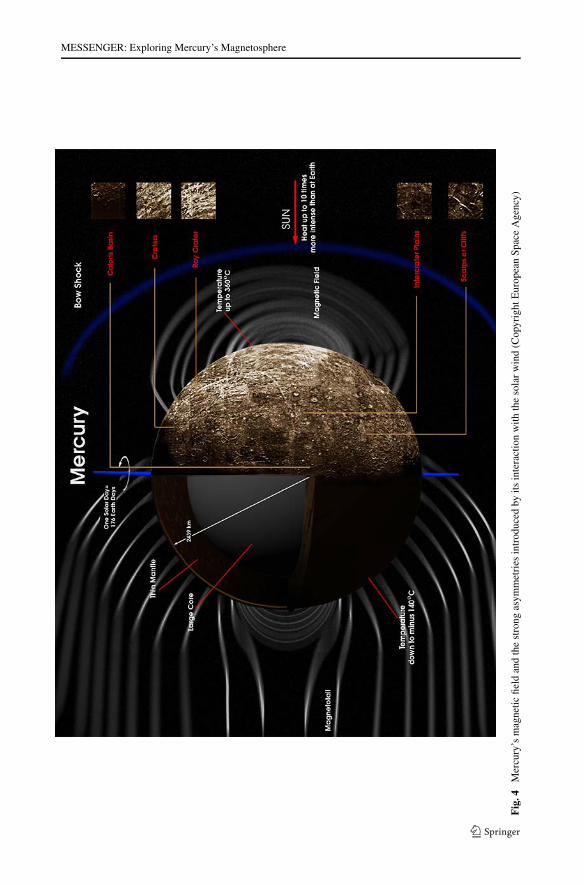
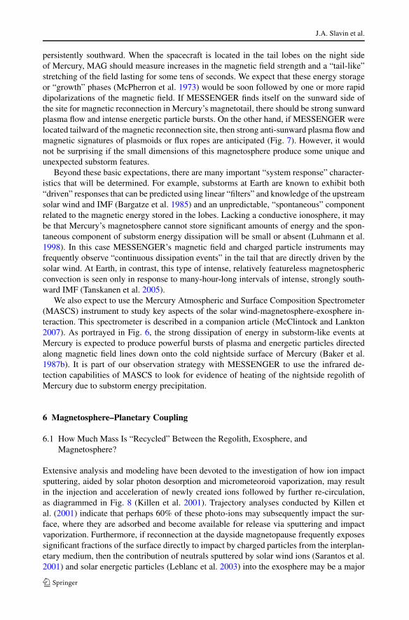
Fig. 7 Schematic depiction of a reconnection-driven substorm within Mercury’s magnetosphere (Slavin2004)

The neutral species in the exosphere travel on ballistic trajectories determined only bygravity and light pressure until the point where they become ionized by solar ultraviolet(UV) radiation, charge exchange with a magnetospheric ion, or electron impact ionization.At that point the newly created ion will begin to execute single particle motion according toits velocity vector at the time of creation and the ambient electric and magnetic fields withinthe magnetosphere (Cheng et al. 1987; Ip 1987; Delcourt et al. 2002, 2003). Alternatively,some of the ions may possess sufficiently large Larmor radii to intersect quickly the mag-netopause or the planet and be lost. For those pickup ions remaining in the magnetosphere,their non-Maxwellian distribution functions will cause plasma waves to be excited, grow,and scatter the ions until they become “thermalized.” The determination of the extent towhich planetary pick-up ions can actually be thermalized within Mercury’s small magne-tosphere is a major objective of MESSENGER. Since Mercury takes 59 days to spin onceabout its axis, planetary rotation is not expected to play any role in particle acceleration ortransport. Hence, the E × B drift or “convection” path for magnetospheric plasma is ex-pected to follow relatively straight lines from the plasma sheet sunward toward the nightsideof the planet and the forward magnetopause, as shown in Fig. 6.

Some of the most energetic charged particles in the tail are thought to be accelerated bythe intense electric fields driven by the reconnection of magnetic flux tubes from the lobes ofthe tail (Hill 1975). At Earth, recently reconnected flux tubes are observed to be bounded by“magnetic separatrices” populated with newly accelerated ions and electrons (Cowley 1980;Scholer et al. 1984). The particles possessing the highest Vparallel are found farthest from thecurrent sheet and closest to the separatrix boundary. These regions of sunward and tailward


streaming energetic charged particles are colored red in Fig. 7. Indeed, short-lived “spikes”in energetic ions and electron flux extending up to at least several MeV have been seenin Earth’s distant magnetotail (Krimigis and Sarris 1979) and have been associated withepisodes of X-line formation and reconnection (Sarris and Axford 1979; Richardson et al.1996). Non-adiabatic processes are necessary to explain these acceleration events, usuallyattributed to the effect of extreme thinning of the cross-tail current sheet relative to theLarmor radii of the ions and electrons (Büchner and Zelenyi 1989; Delcourt et al. 2003;Hoshino 2005).

Many of these accelerated charged particles are immediately lost as they flow down thetail to the interplanetary medium. Others, however, are carried sunward and undergo furtheracceleration due to first invariant conservation. At Earth, ions convected from the inner edgeof the tail may have their energy increased by a factor of 100 by the time they reach the “ringcurrent” region at a radial distance of ∼3 RE from the center of the planet. By contrast, theweak planetary magnetic field at Mercury greatly limits this type of adiabatic acceleration.Indeed, Mercury may be ideal for the direct observation of acceleration associated withX-line formation. As these charged particles approach Mercury and experience strongermagnetic fields, the ions and electrons will begin to experience gradient and curvature driftthat causes the ions to drift about the planet toward dusk while electrons are diverted towarddawn, as indicated in Fig. 6. The loss of these energetic particles via intersection with thesurface of Mercury or the magnetopause is expected to limit severely the flux of quasi-trapped particles that complete a circuit about the planet (Lukyanov et al. 2001; Delcourt etal. 2003), but their loss constitutes an additional source of surface sputtering.

Charged particles also experience acceleration during interactions with ultra-low-frequency (ULF) waves (e.g., Blomberg 1997). Ion pickup due to photo-ionization of neu-trals sputtered from the surface is expected to be a persistent feature of Mercury’s mag-netosphere (Ip 1987). These newly created ions will then experience the convection elec-tric field and be picked up in the plasma flow much as newly ionized atoms are sweptup in the solar wind flow near comets (e.g., Coates et al. 1996). The resulting pickupion distributions contain significant free energy and can be unstable to various cyclotronwave modes, many of which have magnetic signatures in the vicinity of the ion gyro-frequencies (Gomberoff and Astudillo 1998). Cyclotron waves may also be generated byions accelerated in the magnetotail as they convect sunward and are commonplace atEarth (Anderson et al. 1992). At Earth ion populations can also drive long-wavelength,low-frequency waves which, in turn, couple to field-line resonances (e.g., Southwood andKivelson 1981). While the ion gyro-frequencies and field-line resonance frequencies atEarth are separated by a factor of 10 to 100, at Mercury the gyro-frequencies are fairlylow because of the low magnetic field strength at Mercury, while the field-line resonanceperiods should be relatively high owing to the small size of the magnetosphere (Russell1989). The wave-particle physics at Mercury may, therefore, be particularly interesting,because the kinetic and longer wavelength waves should be coupled (Othmer et al. 1999;Glassmeier et al. 2003).

5.2 How Will Energetic Particle Acceleration Processes Be Measured at Mercury?

The EPPS and MAG instruments will be used in concert to explore Mercury’s magne-tosphere, map out its different regions, and determine the spatial and temporal variationsin the charged particle populations peculiar to the different parts of the magnetosphere (seeMukai et al. 2004). For example, the magnetic field and plasma measurements will be usedto calculate the ratio of thermal particle pressure to magnetic pressure, termed the “β” value

J.A. Slavin et al.

of the plasma. The inner regions close to the planet and the lobes of the tail are typicallydominated by the magnetic field pressure and have very low β values, i.e., <0.1. The plasmasheet region (see Fig. 6), in contrast, is dominated by thermal pressure. At Earth the plasmasheet has β values that vary from a few times 0.1 in the outer layers to �10 in the cen-tral portion where the cross-tail electric current density peaks. The most dynamic eventsobserved in the Earth’s magnetosphere, such as “bursty bulk flows” and “dipolarizations,”are generally found in the plasma sheet region (Angelopoulos et al. 1992). Streaming en-ergetic particles accelerated in the separatrices emanating from X-lines are most frequentlyobserved in the outer layers of the plasma sheet where β ∼ 0.1.

The MESSENGER EPPS instrument will provide comprehensive observations of ionsand electrons from low altitudes over the north polar regions (see Fig. 3b) out throughthe lobes and into the cross-tail current layer. The flux of ions moving up and down thesemagnetic flux tubes will be measured directly and used to infer the rate at which mass isexchanged between the surface of the planet and the magnetosphere. Furthermore, any at-tendant acceleration of the charged particles will also be observed. The natural tendency ofenergetic particles to disperse, with faster particles reaching an observer before the slowerparticles, is a strong modeling constraint for determining the source populations, drift paths,and magnetic conjugacies. Modeling and analysis of dispersed ion-injection events at vari-ous distances down the tail at the Earth have shown that it is often possible to specify the timeand location where the initial acceleration event took place (Mauk 1986; Sauvaud et al. 1999;Kazama and Mukai 2005).

The MESSENGER Magnetometer is also designed to characterize waves and wave-particle interactions at Mercury. The MAG instrument provides coverage up to 10 Hz, a bandthat spans all of the relevant ion gyro-frequencies including protons throughout the planetarymagnetosphere. Even during periods of low telemetry allocations the magnetospheric sam-pling will be no coarser than 2 vectors s−1 providing coverage over all ULF and heavy-iongyro-frequencies. Moreover, the MAG provides a burst detection capability that will allowcapture of large-amplitude wave events. In concert with FIPS and EPS observations of iondistributions and composition such measurements will provide a comprehensive survey ofwave activity and determine their correspondence with the local ion populations.

5.3 Do Terrestrial-Style Substorms Occur at Mercury?

Mercury is expected to be one of the best places to test and extend our understandingof magnetospheric substorms. Because of its closeness to the Sun, this magnetosphereis subject to the most intense solar wind pressure and IMF intensity in the solar system(Burlaga 2001). The MESSENGER measurements will give detailed observations of sub-storms in a magnetosphere where planetary rotation is negligible and no ionosphere ispresent. The slow rotation of Mercury will result in sunward convection in the equator-ial region being dominant throughout the forward magnetosphere. This is in stark contrastwith Saturn, the other planet where terrestrial-type substorms are thought to occur. Sat-urn has a rapid rotation that dominates magnetospheric convection to the point where eventhe tail magnetic field may be twisted into a helical configuration (Mitchell et al. 2005;Cowley et al. 2005).

The absence of a collisional ionosphere at Mercury also has important consequencesfor global electric currents and plasma convection. At Earth and Saturn it is believed thatthe timescale for the substorm growth phase is determined by ionospheric line-tying thatin turn limits the rate of magnetic flux circulation from the dayside magnetosphere to thenightside and back again (Coroniti and Kennel 1973). Furthermore, some theories of the


substorm expansion phase at Earth require active feedback between the magnetosphere andan ionosphere whose conductivity varies at least somewhat with the rate of charged particleprecipitation (Baker et al. 1996). Such feedback is presumably absent at Mercury, althoughwe shall evaluate the situation using the MESSENGER observations. In this manner, it willbe determined whether or not active feedback between an ionosphere and the equatorialmagnetosphere is a necessary condition for magnetospheric substorms. Finally, the flowof field-aligned currents to low altitudes produces auroras in the Earth’s upper atmospherewhen the charge carriers impact neutral atoms. It is unlikely that classical auroras wouldoccur at Mercury. Nonetheless, Joule heating due to magnetospheric field-aligned currentsclosing at very shallow depths beneath Mercury’s surface may create a “warm” auroral ovalthat might be visible at infrared wavelengths (Baker et al. 1987b).

Siscoe et al. (1975) and Ogilvie et al. (1977) showed that the energetic particle burstsdetected by Mariner 10 tended to occur at times when the magnetic field exhibited the dis-turbed behavior characteristic of substorms at Earth. Mariner 10 entered the near-tail plasmasheet on the dusk side of the tail during its first Mercury encounter. The magnetic field ob-served inside the magnetopause was very tail-like and relatively quiet during the inboundhalf of the encounter. Shortly after closest approach, |B| decreased rapidly, and the field in-clination increased markedly, becoming less tail-like and more dipole-like. Such magneticfield variations are a classic signature of substorm expansive phase onset at the Earth wherethey are termed “dipolarization events” (Baker et al. 1996). Christon et al. (1987) conductedcomparative studies of the magnetic field changes observed in association with the Mercuryand Earth magnetosphere energetic particle events in the near-tail and found them to beextremely similar.

Siscoe et al. (1975) also called attention to the fact that the IMF switched from north-ward to southward while Mariner 10 was in the magnetosphere. These authors suggested,by analogy to Earth, that this change in IMF direction initiated reconnection at the daysidemagnetopause, magnetic flux transfer to the tail, and, finally, tail reconnection. As shownschematically in Fig. 7, tail reconnection is believed to drive fast plasma flows and energeticparticle acceleration. Indeed, Slavin and Holzer (1979a) found that the altitude of the day-side magnetopause for both M10 encounters was reduced whenever the IMF Bz componentwas southward, consistent with the reconnection model. Siscoe et al. further used scalingarguments to suggest that if substorms occurred at Mercury, then their timescales should beof order 1–2 min, similar to the M10 energetic particle events, in contrast with the ∼1 hrtypical of the Earth’s magnetosphere.

Eraker and Simpson (1986) and Baker et al. (1986) developed this scenario further andsuggested that the substorms in Mercury’s magnetotail resulted from magnetic reconnectionin the range of 3–6 RM on the nightside, as shown in Fig. 7. During substorms in Earth’smagnetosphere, the plasma sheet has been observed to be severed by magnetic reconnectionquite close to Earth, i.e., ∼20–30 RE or ∼2–3 times the solar wind stand-off distance. Thereconnection process produces a magnetically confined structure (i.e., loop-like or helicalmagnetic topology) termed a “plasmoid” (Hones et al. 1984; Slavin et al. 1984) that isejected down the tail at high speed, as schematically depicted in Fig. 7. As at the Earth,the observation of plasmoids in Mercury’s magnetotail would provide direct informationregarding the time of onset and intensity of magnetic reconnection (e.g., Baker et al. 1987a;Slavin et al. 2002).

5.4 How Will Substorm Activity Be Identified in the MESSENGER Measurements?

Given our present understanding of the Mariner 10 observations, we expect that substormsin the MESSENGER data will appear whenever the IMF upstream of Mercury becomes

J.A. Slavin et al.

persistently southward. When the spacecraft is located in the tail lobes on the night sideof Mercury, MAG should measure increases in the magnetic field strength and a “tail-like”stretching of the field lasting for some tens of seconds. We expect that these energy storageor “growth” phases (McPherron et al. 1973) would be soon followed by one or more rapiddipolarizations of the magnetic field. If MESSENGER finds itself on the sunward side ofthe site for magnetic reconnection in Mercury’s magnetotail, there should be strong sunwardplasma flow and intense energetic particle bursts. On the other hand, if MESSENGER werelocated tailward of the magnetic reconnection site, then strong anti-sunward plasma flow andmagnetic signatures of plasmoids or flux ropes are anticipated (Fig. 7). However, it wouldnot be surprising if the small dimensions of this magnetosphere produce some unique andunexpected substorm features.

Beyond these basic expectations, there are many important “system response” character-istics that will be determined. For example, substorms at Earth are known to exhibit both“driven” responses that can be predicted using linear “filters” and knowledge of the upstreamsolar wind and IMF (Bargatze et al. 1985) and an unpredictable, “spontaneous” componentrelated to the magnetic energy stored in the lobes. Lacking a conductive ionosphere, it maybe that Mercury’s magnetosphere cannot store significant amounts of energy and the spon-taneous component of substorm energy dissipation will be small or absent (Luhmann et al.1998). In this case MESSENGER’s magnetic field and charged particle instruments mayfrequently observe “continuous dissipation events” in the tail that are directly driven by thesolar wind. At Earth, in contrast, this type of intense, relatively featureless magnetosphericconvection is seen only in response to many-hour-long intervals of intense, strongly south-ward IMF (Tanskanen et al. 2005).

We also expect to use the Mercury Atmospheric and Surface Composition Spectrometer(MASCS) instrument to study key aspects of the solar wind-magnetosphere-exosphere in-teraction. This spectrometer is described in a companion article (McClintock and Lankton2007). As portrayed in Fig. 6, the strong dissipation of energy in substorm-like events atMercury is expected to produce powerful bursts of plasma and energetic particles directedalong magnetic field lines down onto the cold nightside surface of Mercury (Baker et al.1987b). It is part of our observation strategy with MESSENGER to use the infrared de-tection capabilities of MASCS to look for evidence of heating of the nightside regolith ofMercury due to substorm energy precipitation.

6 Magnetosphere–Planetary Coupling

6.1 How Much Mass Is “Recycled” Between the Regolith, Exosphere, andMagnetosphere?

Extensive analysis and modeling have been devoted to the investigation of how ion impactsputtering, aided by solar photon desorption and micrometeoroid vaporization, may resultin the injection and acceleration of newly created ions followed by further re-circulation,as diagrammed in Fig. 8 (Killen et al. 2001). Trajectory analyses conducted by Killen etal. (2001) indicate that perhaps 60% of these photo-ions may subsequently impact the sur-face, where they are adsorbed and become available for release via sputtering and impactvaporization. Furthermore, if reconnection at the dayside magnetopause frequently exposessignificant fractions of the surface directly to impact by charged particles from the interplan-etary medium, then the contribution of neutrals sputtered by solar wind ions (Sarantos et al.2001) and solar energetic particles (Leblanc et al. 2003) into the exosphere may be a major


Fig. 8 Mass exchange betweenthe solar wind, magnetosphere,exosphere, and regolith atMercury (Killen et al. 2001)

driver for this system. The relatively short times, i.e., hours, required for photo-ionizationand charge exchange will lead to sputtered neutrals being quickly ionized and picked-up bythe convective flow within the magnetosphere to produce a coupled system (see also Fig. 6).

The nature of this complex chain of coupled processes that link the planet to the at-mosphere and the magnetosphere has become a major focus for the Mercury research com-munity. Killen et al. (2001) found that Mercury’s atmosphere is sufficiently tenuous that itwould soon be depleted by losses, if it were not being continuously replenished from be-low as depicted in Fig. 8. The creation of exospheric neutrals involves several competingprocesses including photon desorption, ion sputtering, and meteoritic impact (e.g., Killenand Ip 1999; Milillo et al. 2005). All of these processes and how the MESSENGER measure-ments will contribute to our understanding of them are discussed in detail in a companionarticle (Domingue et al. 2007).

The dynamic nature of Mercury’s magnetosphere is expected to complicate the measure-ment of the rate of recycling of magnetospheric ions and neutrals. After a newly liberatedneutral leaves the surface, it follows a ballistic trajectory until it impacts the surface or be-comes ionized (see review by Hunten et al. 1988). If a given particle becomes ionized thenit will be accelerated by the magnetospheric electric fields until it either collides with theplanetary surface or is thermalized and swept along by the convective flow in the equatorialmagnetosphere. The exospheric neutrals available for ionization depend heavily on the com-position of the planetary surface. Charged particle and photon sputtering work on the firstfew monolayers of the surface grains, so pre-sputtered atoms must first make their way to themonolayers by diffusion. Gardening rates for the crust are much faster than the time required

J.A. Slavin et al.

to deplete a grain of a given species, providing a constant supply of neutrals to the exosphere(see Killen et al. 2004). On the basis of the Mariner 10 observations, the magnetosphericreconfiguration time is only a few minutes (Siscoe et al. 1975; Slavin and Holzer 1979a;Luhmann et al. 1998). Hence, the trajectories of magnetospheric ions through the magne-tosphere may be quite complex (Delcourt et al. 2002).

Several studies have been performed that examine the importance of ion recycling inMercury’s exosphere and magnetosphere (e.g., Zurbuchen et al. 2004). Koehn (2002) usedthe MHD model of Kabin et al. (2000) to study the surface-to-surface transport of OH+and S+ ions. For normal solar wind conditions, he found that ions created at mid-latitudestended to return to equatorial dusk regions, while ions formed elsewhere were lost to themagnetosphere and solar wind. For very strong solar wind conditions, returning ions tendedto move poleward and duskward, enhancing mid-latitude regions. Recycling rates for thisstudy were less than 10%.

Delcourt et al. (2003) and Leblanc et al. (2003) followed the trajectories of Na+ ionswith an initial energy of 1 eV using a realistic magnetospheric magnetic field model. Theirresults show Na+ returning to the surface primarily along two mid-latitude regions centeredon ±30◦, with some returning to duskside latitudes equatorward of ±20◦. Recycling ratesfor these studies were 10–15%. Killen et al. (2004) utilized a new model (see Sarantos etal. 2001) that, unlike that of Delcourt et al. (2003), takes into account radial magnetic fieldorientation. Their ion initial energies were also ∼1 eV. The measured recycling rates aresignificantly higher (60%), and they find that dawnside-generated ions tend to return to thesurface, while duskside-born ions are swept away by the solar wind.

6.2 How Will the MESSENGER Observations Be Used to Discover the Extent of MassExchange Between Mercury’s Regolith, Exosphere, and Magnetosphere?

Perhaps no science objective will so fully utilize the MESSENGER instruments as thestudy of the mass exchange between the planetary surface, exosphere, and magnetosphere.The MAG instrument will map the magnetic field, providing insight into magnetosphericdynamics and supporting improved field models. The Gamma-Ray and Neutron Spec-trometer (GRNS) and X-Ray Spectrometer (XRS) instruments (Goldsten et al. 2007;Schlemm et al. 2007) will provide elemental composition maps of the surface, from whichexospheric neutrals arise, forming the seed population for magnetospheric ions. MASCSwill measure the composition of the neutral atmosphere, recently liberated from the re-golith. EPPS will detect pickup ions in the magnetosphere and then map detected ions backto surface regions from which they escaped. The Mercury Dual Imaging System (MDIS)instrument (Hawkins et al. 2007) will then image the surface from which these neutrals andions are sputtered, thereby tying atmospheric and magnetospheric measurements back tosurface features.

In addition, EPPS and MAG will allow us to understand the complex interplay betweenmagnetospheric plasmas and the magnetic field. In the event that the magnetopause is com-pressed sufficiently such that the solar wind can come into direct contact with much of thesurface, EPPS will monitor the likely large increase in exospheric neutrals and newly cre-ated magnetospheric ions. Large increases in the rate of ion sputtering from the surface hasbeen offered as a likely explanation for the high degree of temporal and spatial variationin Mercury’s atmosphere as observed from the Earth (Potter et al. 1999). Such increaseswould soon lead to a large number of new photo-ions that can modify the magnetosphericconfiguration, which MAG can also detect. In summary, most aspects of the recycling ofmagnetospheric ions between the exosphere and surface are still very much open issues.


The MESSENGER instrument payload will make the critical measurements that will re-solve the most important questions regarding the mass exchange within this closely coupledsystem.

6.3 Do Field-Aligned Currents Couple Mercury to Its Magnetosphere, and How Do TheyClose?

Among the fundamental aspects of all planetary magnetospheres visited thus far are field-aligned electric currents (Kivelson 2005). When magnetospheric magnetic fields reconnectwith the IMF and are pulled back into the tail at Earth, sheets of field-aligned current, termed“Region 1” currents, flow down into the high-latitude ionosphere on the dawn side of thepolar cap and outward on the dusk side. These Region 1 currents are also expected to bepresent at Mercury, as schematically depicted in Fig. 9, though their intensity and temporalevolution may be greatly modified depending upon the nature of current closure path and theelectrical conductivity of the regolith (Slavin et al. 1997). When the magnetic flux tubes inthe tail reconnect again and high-speed plasma jets are generated toward and away from theplanet (see Fig. 7), another set of field-aligned currents are generated, termed the “substormcurrent wedge (SCW)” (McPherron et al. 1973; Hesse and Birn 1991; Shiokawa et al. 1998).These currents are also shown in Fig. 9. The SCW currents connect the midnight region ofthe polar cap to the plasma sheet and transfer to the planet a significant fraction of the totalenergy being released in the tail (e.g., Fedder and Lyon 1987). These SCW currents are themost likely source of the field-aligned currents in the Mariner 10 measurements reportedby Slavin et al. (1997). Numerical simulations by Janhunen and Kallio (2004) and Ip andKopp (2004) suggest that Region 1 and SCW field-aligned currents will have importantconsequences for the structure of Mercury’s magnetosphere as they do for that of Earth(cf. Fedder and Lyon 1987). However, in order for these currents to reach a steady-state,they must have a conductive path for closure. As Mercury possesses no such conductiveionosphere, other mechanisms or paths must be found.

A moderately conductive regolith is a likely candidate for FAC closure at Mercury. Hillet al. (1976) suggested a conductance value of 0.1 mho, which is not unreasonable basedupon the lunar measurements. If this value were indeed appropriate, however, the highrate of joule heating in the regolith would severely limit the duration of the current flowas the available magnetospheric energy would be quickly dissipated. Cheng et al. (1987)showed that sputtering is a possible means to generate the neutral sodium atmosphere ofMercury and a source population for magnetospheric ions. They further pointed out thatthe new ions created by photo-ionization, electron impact ionization, and charge exchangeare available to be “picked-up” by the convective motion of the magnetospheric flux tubes(Fig. 6). In doing so, they would give rise to a “pickup” or “mass loading” conductance (seeKivelson 2005) that might contribute to the generation and/or closure of FACs at Mercury.Photoelectrons have also been suggested as a source of current carriers (Grard et al. 1999;Grard and Balogh 2001). However, the pick-up of planetary ions and the photoelectronsheath over Mercury’s sunlit surface provide conductances that are only slightly greaterthan the lunar values. Measurements of surface characteristics, as well as neutral andion populations near the surface of Mercury, are necessary for a better understanding ofmagnetosphere-surface coupling. Glassmeier (2000) argued that field-aligned currents atMercury may close as diamagnetic currents in regions of enhanced plasma density nearthe planet; for example, at low altitudes over the nightside of the Mercury where sunward-directed, reconnection-driven fast flows encounter strong planetary magnetic field. Janhunenand Kallio (2004) considered possible surface materials and mineralogy and concluded that

J.A. Slavin et al.

Fig. 9 Depiction of possible Region 1 and substorm current wedge field-aligned currents at high latitudes.Subsurface solar wind induction currents, flowing in the planetary interior, are shown at lower latitudes

the effective height-integrated conductance could fall within a wide range. In summary, thenew, more detailed measurements to be returned by MESSENGER are necessary beforethe nature of the electrodynamic coupling between Mercury, its atmosphere, and its magne-tosphere can be determined.

6.4 How Will MESSENGER Detect and Map Field-Aligned Currents and Determine TheirClosure Path?

The large-scale field-aligned currents at Mercury should be readily detected by MESSEN-GER’s instrumentation. The signatures of currents at low altitudes in the Earth systemare well known (Iijima and Potemra 1978; Zanetti and Potemra 1982). The low-altitudenorthern hemisphere portion of the MESSENGER orbit, as depicted in Figs. 3a and 3b,is ideal for detecting field-aligned currents since the magnetic perturbation scales as r−3/2

(Rich et al. 1990). Experience at the Earth shows that single spacecraft measurements pro-vide accurate field-aligned current determinations using the infinite-current-sheet assump-tion (Rich et al. 1990; Anderson et al. 1998, 2000). Although this approach breaks downmore than a few hours from dawn and dusk and under other circumstances (e.g., northward


IMF) when fringing effects dominate the signatures, the magnetic signatures unambigu-ously indicate the presence of the currents even if one cannot confidently infer the cur-rent density distribution from the data (cf. Fung and Hoffman 1992; Waters et al. 2001;Korth et al. 2005). In addition, particle data provide useful correlative observations of thecurrent carriers, and the FIPS and EPS sensors which measure composition, velocity, anddensity for both ions and electrons will, in principle, give a direct measurement of current.As most current carriers are of relatively low energy, the broad energy range of EPPS willbe of particular importance. Finally, GRNS, XRS, and other instruments will provide dataabout the makeup of the regolith, allowing better estimates of the surface conductivity.

7 Summary

A common paradigm describing the accumulation of knowledge about a planetary bodysuggests that advances come in four mission phases: “reconnaissance,” “exploration,” “in-tensive study,” and “understanding.” Applied to Mercury, the Mariner 10 mission can besaid to have contributed to our progress by providing a reconnaissance-level characteriza-tion. In particular, those measurements showed that Mercury possesses an intrinsic magneticfield that interacts strongly with the solar wind, especially when the IMF is southward, andproduces short-duration, intense variations in the tail magnetic field that are well correlatedwith energetic particle acceleration events.

As described here, the MESSENGER mission will explore Mercury’s magnetic field andits magnetosphere for the first time. The mission will determine whether the planet’s mag-netic field is the result of an ongoing convective dynamo, some other type of dynamo, orcrustal magnetization. MESSENGER will also characterize the structure and dynamics ofMercury’s magnetosphere and its response to average and extreme interplanetary conditions.In particular, it will determine whether Earth-like “substorms” occur, how the lack of anionosphere affects magnetospheric dynamics, and the processes responsible for Mercury’sintense energetic particle acceleration events. Moreover, the mission will determine the na-ture and importance of the coupling between this magnetosphere, the exosphere, and theregolith and, via induction effects, the planetary interior. The importance of magnetosphericcharged particle precipitation for the maintenance and variability of the exosphere will bedetermined. Conversely, the impact of newly formed heavy ions due to the ionizing effects ofsolar extreme-UV radiation on the exosphere will also be measured. Finally, the existenceof field-aligned currents and the nature of their low-altitude closure will be revealed. Thesuccess of MESSENGER in achieving these exploration-level, and some intensive-study,objectives will, in turn, produce a foundation for the comprehensive investigations to be car-ried out by future missions, such as BepiColombo (Grard and Balogh 2001), that will yielda detailed understanding of this most intriguing magnetosphere.

Acknowledgements The authors express their great appreciation to all of those who have contributed to theMESSENGER mission. Useful comments and discussion with J. Eastwood, M. Sarantos, and S. Boardsen,are also gratefully acknowledged.

References

M.H. Acuña et al., Science 279, 1676–1680 (1998)M.H. Acuña et al., Science 284, 790–793 (1999)O. Aharonson, M.T. Zuber, S.C. Solomon, Earth Planet. Sci. Lett. 218, 261–268 (2004)

J.A. Slavin et al.

B.J. Anderson et al., Space Sci. Rev. (2007, this issue)B.J. Anderson, R.E. Erlandson, L.J. Zanetti, J. Geophys. Res. 97, 3075–3088 (1992)B.J. Anderson, J.B. Gary, T.A. Potemra, R.A. Frahm, J.R. Sharber, J.D. Winningham, J. Geophys. Res. 103,

26323–26335 (1998)B.J. Anderson, K. Takahashi, B.A. Toth, Geophys. Res. Lett. 27, 4045–4048 (2000)G.B. Andrews et al., Space Sci. Rev. (2007, this issue)V. Angelopoulos et al., J. Geophys. Res. 97, 4027–4039 (1992)T.P. Armstrong, S.M. Krimigis, L.J. Lanzerotti, J. Geophys. Res. 80, 4015–4017 (1975)D.N. Baker, J.A. Simpson, J.H. Eraker, J. Geophys. Res. 91, 8742–8748 (1986)D.N. Baker, R.C. Anderson, R.D. Zwickl, J.A. Slavin, J. Geophys. Res. 92, 71–81 (1987a)D.N. Baker et al., J. Geophys. Res. 92, 4707–4712 (1987b)D.N. Baker, T.I. Pulkkinen, V. Angelopoulos, W. Baumjohann, R.L. McPherron, J. Geophys. Res. 101,

12975–13010 (1996)L.F. Bargatze, D.N. Baker, R.L. McPherron, E.W. Hones Jr., J. Geophys. Res. 90, 6387–6394 (1985)T.A. Bida, R.M. Killen, T.H. Morgan, Nature 404, 159–161 (2000)L.G. Blomberg, Planet. Space Sci. 45, 143–148 (1997)A.L. Broadfoot, D.E. Shemansky, S. Kumar, Geophys. Res. Lett. 3, 577–580 (1976)J. Büchner, L.M. Zelenyi, J. Geophys. Res. 94, 11821–11842 (1989)L.F. Burlaga, Planet. Space Sci. 49, 1619–1627 (2001)A.F. Cheng, R.E. Johnson, S.M. Krimigis, L.J. Lanzerotti, Icarus 71, 430–440 (1987)S.P. Christon, Icarus 71, 448–471 (1987)S.P. Christon, J. Feynman, J.A. Slavin, in Magnetotail Physics, ed. by A.T.Y. Lui (Johns Hopkins University

Press, Baltimore, 1987), pp. 393–402A.J. Coates, A.D. Johnstone, F.M. Neubauer, J. Geophys. Res. 101, 27573–27584 (1996)J.E.P. Connerney, N.F. Ness, in Mercury, ed. by F. Vilas, C.R. Chapman, M.S. Matthews (University of

Arizona Press, Tucson, 1988), pp. 494–513F.V. Coroniti, C.F. Kennel, J. Geophys. Res. 78, 2837–2851 (1973)S.W.H. Cowley, Space Sci. Rev. 25, 217–275 (1980)S.W.H. Cowley et al., J. Geophys. Res. 110, A02201 (2005). doi: 10.1029/2004JA010796D.C. Delcourt, T.E. Moore, S. Orsini, A. Millilo, J.-A. Sauvaud, Geophys. Res. Lett. 29, 1591 (2002). doi:

10.1029/2001GL013829D.C. Delcourt et al., Ann. Geophys. 21, 1723–1736 (2003)D.L. Domingue et al., Space Sci. Rev. (2007, this issue)J.H. Eraker, J.A. Simpson, J. Geophys. Res. 91, 9973–9993 (1986)J.A. Fedder, J.G. Lyon, Geophys. Res. Lett. 14, 880–883 (1987)S.F. Fung, R.A. Hoffman, J. Geophys. Res. 97, 8569–8579 (1992)G. Giampieri, A. Balogh, Planet. Space Sci. 49, 1637–1642 (2001)G. Giampieri, A. Balogh, Planet. Space Sci. 50, 757–762 (2002)K.-H. Glassmeier, in Magnetospheric Current Systems, ed. by S.-I. Ohtani, R. Fujii, M. Hesse, R.L. Lysak.

Geophysical Mon., vol. 118 (American Geophysical Union, Washington, 2000), pp. 371–380K.-H. Glassmeier, N.P. Mager, D.Y. Klimushkin, Geophys. Res. Lett. 30, 1928 (2003). doi:

10.1029/2003GL017175R.E. Gold et al., Planet. Space Sci. 49, 1467–1479 (2001)J.O. Goldsten et al., Space Sci. Rev. (2007, this issue)B.E. Goldstein, S.T. Suess, R.J. Walker, J. Geophys. Res. 86, 5485–5499 (1981)L. Gomberoff, H.F. Astudillo, Planet. Space Sci. 46, 1683–1687 (1998)R. Grard, A. Balogh, Planet. Space Sci. 49, 1395–1407 (2001)R. Grard, H. Laakso, T.I. Pulkkinen, Planet. Space Sci. 47, 1459–1463 (1999)J. Grosser, K.-H. Glassmeier, S. Stadelmann, Planet. Space Sci. 52, 1251–1260 (2004)S.E. Hawkins III, et al., Space Sci. Rev. (2007, this issue)M. Hesse, J. Birn, J. Geophys. Res. 96, 19417–19426 (1991)T.W. Hill, J. Geophys. Res. 80, 4689–4699 (1975)T.W. Hill, A.J. Dessler, R.A. Wolf, Geophys. Res. Lett. 3, 429–432 (1976)R.E. Holzer, J.A. Slavin, J. Geophys. Res. 83, 3831–3839 (1978)E.W. Hones Jr. et al., Geophys. Res. Lett. 11, 5–7 (1984)H. Hoshino, J. Geophys. Res. 110, A102154 (2005). doi: 10.1029/2005JA011229L.L. Hood, G. Schubert, J. Geophys. Res. 84, 2641–2647 (1979)D.M. Hunten, T.H. Morgan, D.E. Schemansky, in Mercury, ed. by F. Vilas, C.R. Chapman, M.S. Matthews

(University of Arizona Press, Tucscon, 1988), pp. 562–612T. Iijima, T.A. Potemra, J. Geophys. Res. 83, 599–615 (1978)W.-H. Ip, Icarus 71, 441–447 (1987)

http://dx.doi.org/10.1029/2004JA010796

http://dx.doi.org/10.1029/2001GL013829

http://dx.doi.org/10.1029/2003GL017175

http://dx.doi.org/10.1029/2005JA011229


W.-H. Ip, A. Kopp, J. Geophys. Res. 107, 1348 (2002). doi: 10.1029/2001JA009171W.-H. Ip, A. Kopp, Adv. Space. Res. 33, 2172–2175 (2004)D.J. Jackson, D.B. Beard, J. Geophys. Res. 82, 2828–2836 (1977)P. Janhunen, E. Kallio, Ann. Geophys. 22, 1829–1830 (2004)K. Kabin, T.I. Gombosi, D.L. DeZeeuw, K.G. Powell, Icarus 143, 397–406 (2000)Y. Kazama, T. Mukai, J. Geophys Res. 110, A07213 (2005). doi: 10.1029/2004JA010820R.M. Killen, W.-H. Ip, Rev. Geophys. Space Phys. 37, 361–406 (1999)R.M. Killen et al., J. Geophys. Res. 106, 20509–20525 (2001)R.M. Killen, M. Sarantos, A.E. Potter, P.H. Reiff, Icarus 171, 1–19 (2004)M.G. Kivelson, Space Sci. Rev. 116, 299–318 (2005)P.L. Koehn, Ph.D. Thesis, University of Michigan, Ann Arbor, 2002H. Korth et al., Planet. Space Sci. 54, 733–746 (2004)J. Korth, B.J. Anderson, Frey, C.L. Waters, Ann. Geophys. 23, 1295–1310 (2005)S.M. Krimigis, E.T. Sarris, in Dynamics of the Magnetosphere, ed. by S.-I. Akasofu (Reidel, Dordrecht,

1979), pp. 599–630H. Lammer, S.J. Bauer, Planet. Space Sci. 45, 73–79 (1997)H. Lammer et al., Icarus 166, 238–247 (2003)F. Leblanc, J.G. Luhmann, R.E. Johnson, M. Lui, Planet. Space Sci. 51, 339–352 (2003)J.G. Luhmann, C.T. Russell, N.A. Tsyganenko, J. Geophys. Res. 103, 9113–9119 (1998)A.V. Lukyanov, S. Barabash, R. Lundin, P.C. Brandt, Planet. Space Sci. 49, 1677–1684 (2001)S. Massetti et al., Icarus 166, 229–237 (2003)B.H. Mauk, J. Geophys. Res. 91, 13423–13431 (1986)W. McClintock, M.R. Lankton, Space Sci. Rev. (2007, this issue)R.L. McPherron, C.T. Russell, M.P. Aubry, J. Geophys. Res. 78, 3131–3149 (1973)A. Milillo et al., Space Sci. Rev. 117, 397–443 (2005)D.G. Mitchell et al., Geophys. Res. Lett. 32, L20S01 (2005). doi: 10.1029/2005GL022647T. Mukai, K. Ogasawara, Y. Saito, Adv. Space Res. 33, 2166–2171 (2004)N.F. Ness, in Solar System Plasma Physics, vol. II, ed. by C.F. Kennel, L.J. Lanzerotti, E.N. Parker (North-

Holland, New York, 1979), pp. 185–206N.F. Ness, K.W. Behannon, R.P. Lepping, Y.C. Whang, K.H. Schatten, Science 185, 151–160 (1974)N.F. Ness, K.W. Behannon, R.P. Lepping, J. Geophys. Res. 80, 2708–2716 (1975)N.F. Ness, K.W. Behannon, R.P. Lepping, Y.C. Whang, Icarus 28, 479–488 (1976)K.W. Ogilvie et al., Science 185, 145–150 (1974)K.W. Ogilvie, J.D. Scudder, V.M. Vasyliunas, R.E. Hartle, G.L. Siscoe, J. Geophys. Res. 82, 1807–1824

(1997)C. Othmer, K.-H. Glassmeier, R. Cramm, J. Geophys. Res. 104, 10369–10378 (1999)A.E. Potter, T.H. Morgan, Science 229, 651–653 (1985)A.E. Potter, T.H. Morgan, Icarus 67, 336–340 (1986)A.E. Potter, R.M. Killen, T.H. Morgan, Planet. Space Sci. 47, 1441–1448 (1999)F.J. Rich, D.A. Hardy, R.H. Redus, M.S. Gussenhoven, J. Geophys. Res. 95, 7893–7913 (1990)I.G. Richardson, C.J. Owen, J.A. Slavin, J. Geophys. Res. 101, 2723–2740 (1996)S.K. Runcorn, Nature 253, 701–703 (1975a)S.K. Runcorn, Phys. Earth Planet. Inter. 10, 327–335 (1975b)C.T. Russell, Geophys. Res. Lett. 4, 387–390 (1977)C.T. Russell, R.J. Walker, J. Geophys. Res. 90, 11067–11074 (1985)C.T. Russell, D.N. Baker, J.A. Slavin, in Mercury, ed. by F. Vilas, C.R. Chapman, M.S. Matthews (University

of Arizona Press, Tucscon, 1988), pp. 514– 561C.T. Russell, Geophys. Res. Lett. 16, 1253–1256 (1989)A.G. Santo et al., Planet. Space Sci. 49, 1481–1500 (2001)M. Sarantos, P.H. Reiff, T.W. Hill, R.M. Killen, A.L. Urquhart, Planet. Space Sci. 49, 1629–1635 (2001)E.T. Sarris, W.I. Axford, Nature 77, 460–462 (1979)S. Sasaki, E. Kurahashi, Adv. Space. Res. 33, 2152–2155 (2004)J.-A. Sauvaud et al., J. Geophys. Res. 104, 28565–28586 (1999)C.E. Schlemm II et al., Space Sci. Rev. (2007, this issue)M. Scholer, G. Gloecker, B. Klecker, F.M. Ipavich, D. Hovestadt, E.J. Smith, J. Geophys. Res. 89, 6717–6727

(1984)K. Shiokawa et al., J. Geophys. Res. 103, 4491–4507 (1998)D.G. Sibeck, R.E. Lopez, E.C. Roelof, J. Geophys. Res. 96, 5489–5495 (1991)J.A. Simpson, J.H. Eraker, J.E. Lamport, P.H. Walpole, Science 185, 160–166 (1974)G.L. Siscoe, L. Christopher, Geophys. Res. Lett. 2, 158–160 (1975)G.L. Siscoe, N.F. Ness, C.M. Yeates, J. Geophys. Res. 80, 4359–4363 (1975)

http://dx.doi.org/10.1029/2001JA009171

http://dx.doi.org/10.1029/2004JA010820

http://dx.doi.org/10.1029/2005GL022647

J.A. Slavin et al.

J.A. Slavin, Adv. Space Res. 33, 1587–1872 (2004)J.A. Slavin, R.E. Holzer, J. Geophys. Res. 84, 2076–2082 (1979a)J.A. Slavin, R.E. Holzer, Phys. Earth Planet. Inter. 20, 231–236 (1979b)J.A. Slavin, R.E. Holzer, J. Geophys. Res. 86, 11401–11418 (1981)J.A. Slavin, C.J. Owen, J.E.P. Connerney, S.P. Christon, Planet. Space Sci. 45, 133–141 (1997)J.A. Slavin et al., Geophys. Res. Lett. 11, 657–660 (1984)J.A. Slavin et al., J. Geophys. Res. 107, 1106 (2002). doi: 10.1029/2000JA003501S.C. Solomon, Icarus 28, 509–521 (1976)S.C. Solomon et al., Planet. Space Sci. 49, 1445–1465 (2001)S.C. Solomon, R.L. McNutt Jr., R.E. Gold, D.L. Domingue, Space Sci. Res. (2007, this issue)D.J. Southwood, M.G. Kivelson, J. Geophys. Res. 86, 5643–5655 (1981)L.J. Srnka, Phys. Earth Planet. Inter. 11, 184–190 (1976)A. Stephenson, Earth Planet. Sci. Lett. 28, 454–458 (1976)D.J. Stevenson, Rep. Prog. Phys. 46, 555–620 (1983)D.J. Stevenson, Earth Planet. Sci. Lett. 82, 114–120 (1987)D.J. Stevenson, T. Spohn, G. Schubert, Icarus 54, 466–489 (1983)S.T. Suess, B.E. Goldstein, J. Geophys. Res. 84, 3306–3312 (1979)T. Terasawa et al., Geophys. Res. Lett. 24, 935–938 (1997)E.I. Tanskanen et al., J. Geophys. Res. 110, A03216 (2005). doi: 10.1029/2004JA010561C.L. Waters, B.J. Anderson, K. Liou, Geophys. Res. Lett. 28, 2165–2168 (2001)Y.C. Whang, J. Geophys. Res. 82, 1024–1030 (1977)L.J. Zanetti, T.A. Potemra, Geophys. Res. Lett. 9, 349–352 (1982)M.T. Zuber et al., Space Sci. Rev. (2007, this issue)T.H. Zurbuchen, P. Koehn, Fisk, T. Gombosi, G. Gloeckler, K. Kabin, Adv. Space Res. 33, 1884–1889 (2004)

http://dx.doi.org/10.1029/2000JA003501

http://dx.doi.org/10.1029/2004JA010561

MESSENGER: Exploring Mercury’s...

Documents

Transcript of MESSENGER: Exploring Mercury’s...