Meshfree First-order System Least...

NUMERICAL MATHEMATICS: Theory, Methods and Applications

Numer. Math. Theor. Meth. Appl., Vol. 1, No. 1, pp. 29-43 (2008)

Meshfree First-order System Least Squares

Hugh R. MacMillan1,∗, Max D. Gunzburger2 and John V. Burkardt3

1 Department of Mathematical Sciences, Clemson University, Clemson,

SC 29634-0975, USA.2 School of Computational Science, Florida State University, Tallahassee,

FL 32306-4120, USA.3 Advanced Research Computing, Virginia Tech University, Blacksburg,

VA 24061-0123, USA.

Received 4 December, 2007; Accepted (in revised version) 11 December, 2007

Abstract. We prove convergence for a meshfree first-order system least squares (FOSLS)

partition of unity finite element method (PUFEM). Essentially, by virtue of the partition

of unity, local approximation gives rise to global approximation in H(div) ∩ H(curl).

The FOSLS formulation yields local a posteriori error estimates to guide the judicious

allotment of new degrees of freedom to enrich the initial point set in a meshfree dis-

cretization. Preliminary numerical results are provided and remaining challenges are

discussed.

AMS subject classifications: 65N30, 65N50

Key words: Meshfree methods, first-order system least squares, adaptive finite elements.

1. Introduction

1.1. Summary

Interest remains in avoiding the proper tessellation of a computational domain used

to solve partial differential equations, especially in the context of moving meshfree, or

meshless, particle methods. However, as will be made clear, the flexibility inherent to

using merely the cover of a domain does not come without cost. A number of mostly-

related meshfree approaches have been proposed, yielding a variety of approximation

spaces from which to choose. For example, consider the diffuse element method (DEM),

element free Galerkin (EFG), finite point method (FPM), HP clouds, meshfree local Petrov

Galerkin (MLPG), smooth particle hydrodynamics (SPH), moving least squares SPH (ML-

SPH), material-point method (MPM), partition of unity finite element method (PUFEM),

reproducing kernel particle method (RKPM); see [1,2] for a classification and review. Be-

low, we employ the partition unity (PU) approach, given its flexibility and local nature, to

discretize the prototypical first-order system least-squares (FOSLS) formulation for Pois-

son’s equation. This synthesis can be generalized to existing FOSLS formulations of more

∗Corresponding author. Email address: hma mil lemson.edu (H. R. MacMillan)

http://www.global-sci.org/nmtma 29 c©2008 Global-Science Press

30 H. R. MacMillan, M. D. Gunzburger and J. V. Burkardt

complicated PDE systems. Since the FOSLS formulation presents local a posteriori error

estimates to guide adaptive enrichment of an initially-sparse point set, the synthesis may

enhance the utility of meshfree methods.

Below, after a brief discussion about meshfree methods, we introduce FOSLS and a

vector PUFEM discretization. Then, convergence is proved from assumptions about the lo-

cal approximation spaces defined on each patch used to cover the domain. Finally, several

numerical examples are provided.

1.2. Meshfreedom

The notion of altogether avoiding a mesh requires some clarification. First, a set of

points in a domain, along with an associated covering of the domain, must be chosen.

Given generic specifications for this covering, such as the density used in point set selec-

tion and the degree of overlap, a provision of points and their associated patches can be

supplied probabilistically, without use of a background mesh [3]. However, enrichment

of an initially sparse (or coarse) point set nevertheless entails relaxation of the new point

set, in concert with updating the associated cover. While explicit retriangulation is thus

avoided, significant refinement costs persist to ensure that both point placement and patch

size are suitable.

Integration during assembly of the discrete problem leads to a second unavoidable com-

putational cost. In lieu of a tessellation, integration over each intersecting pair of patches

entails defining quadrature points either locally, in a consistent and efficient manner, or

globally, appealing to some background mesh. Below we simply use circular patches Ωi to

cover a domain Ω ⊂ R2. Rather than perform quadrature on each individual lens, Ωi ∩Ω j,

which would yield a symmetric linear system, it is more efficient to simply set a quadrature

rule on each Ωi. Of course, this leads to an asymmetric system due to inexact integration,

i.e., Ai j is computed using quadrature on Ωi while A j i is computed using quadrature on Ω j.

Our approach is truly meshfree in the sense that integration is performed according

to neighbor connectivity, point locations, and neighboring support radii, not according to

the elements of a tessellation. No background mesh is utilized. As a result, adding and/or

moving individual points is unencumbered by the need to re-tessellate the domain. This

flexibility comes with less-efficient assembly of the discrete problem, primarily because

there are many more regions of overlap, Ωi ∩Ω j, than there are elements of a comparable

tessellation. This cost is compounded by the partition of unity construction, which yields

conforming discretizations at the expense of pointwise conditions on the degree of overlap;

e.g., requiring that each point be covered by at least three elements of the cover, # j|Ωi ∩Ω j 6= ; approaches 30 in Fig. 1.

2. A FOSLS partition of unity method

FOSLS has been applied to far more difficult PDE systems than the simplistic elliptic

problem considered below [4]. As a methodology, it is only distinct from least-squares

(LS) in that a residual on vorticity, or the curl of velocity, is introduced in lieu of solving for

Meshfree First-order System Least Squares 31

pressure; the latter is the common velocity-pressure formulation, while the former leads to

approximation of velocity with respect to H(div)∩H(curl).

2.1. Flux-vorticity formulation

Consider the prototypical first-order system,

−∇ ·u = f in Ω, (2.1)

∇× u= 0 in Ω, (2.2)

n · u = 0 on ΓN , (2.3)

τ · u = 0 on ΓD, (2.4)

where u ∈ H(div;Ω)∩H(curl;Ω) and f ∈ L2(Ω). The simplest FOSLS (L2) approach is to

formulate the solution of system (2.1-2.4) as the minimizer of the interior functional

J (u; f ) :=

‖∇ · u+ f ‖20,Ω+ ‖∇× u‖2

0,Ω

1/2

. (2.5)

By design [4], this functional provides a norm on the space

W=

(

v ∈ H(div;Ω)∩H(curl;Ω) | n · v= 0 on ΓN , τ · v= 0 on ΓD, and

∫

ΓD

τ · v= 0

)

.

That is,

‖v‖W :=J (v; 0,0) =p

⟨L v, L v⟩0,Ω , (2.6)

where

L =

−∇· 0

0 ∇×

.

Note that the (L2(Ω))2-innerproduct is conducted componentwise. Hence, solving for

u= arg minv∈WJ (v; f ) (2.7)

is equivalent to minimizing error in the W-norm. As is standard, defining functionals

F (u,v) = ⟨Lu,L v⟩0,Ω , (2.8)

ℓ(v) =

( f 0)t,L v

0,Ω. (2.9)

leads to a variational form of minimization problem (2.7):

Find u ∈W such that F (u,v) = ℓ(v) for all v ∈W. (2.10)

Motivation for this approach is two-fold. First, functional equivalence to an H1-like

norm implies optimal performance of multigrid methods in solving the resulting discrete

problem. Furthermore, a posteriori W-norm error estimates follow simply from evaluating

the FOSLS functional given a computed solution. In [5], a meshfree LS formulation of


steady incompressible viscous flow is presented that uses a background mesh for integra-

tion and employs RKPM to achieve exact approximation of quadratic functions defined on

the entire domain. We have chosen to avoid any background mesh and focus on retaining

the capacity to enhance a given mesh locally through direct appeal to FOSLS a posteriori

error estimates.

We now establish convergence for problem (2.10) when using a vector partition of

unity to define a discrete subspace of W. We only consider Ω ⊂ R2 and use the notation

∇⊥ ·u = k · (∇× u), but extension to 3-D is straightforward. Non-homogeneous boundary

conditions can be handled through standard lifting techniques or by adding appropriate

boundary terms to (2.5). As will be illustrated, the latter gives rise questions as to the

implementation of Sobolev norms on boundary spaces.

2.2. Vector PU Discretization

Briefly, a scalar partition of unity discretization involves first choosing a set of points in

the domain, ziNi=1, and then determining corresponding supports, Ωi, to constitute a cover,

C = ΩiNi=1| ∪N

i=1Ωi ⊃ Ω . Next, a smooth compactly supported “window function”

is chosen from which a Shephard partition of unity, subordinate to C , is constructed.

Analogous to standard p-refinement, local approximation spaces on each support can then

be formed to improve approximation accuracy.

As discussed in [3], we determine a point set ziNi=1= (x i, yi)Ni=1

along with associated

radii riNi=1to determine C = ΩiNi=1

according to

Ωi = z ∈ R2 | |z− zi| ≤ ri .

Fig. 1 illustrates the connectivity of neighboring patches for such a cover, given a point set

with uniform density.

Figure 1: A point set zi and an illustration of support overlaps given a over of the domain withri = 1.7/

pN . All pat hes Ωik

that interse t the two sele ted Ωi are pi tured. Pat hes that happen tooverlap the boundary appear in red .


Following [6], on each patch we use a quartic spline window function

ω(s) =

¨

1− 6s2 + 8s3 − 3s4 for 0≤ s ≤ 1,

0 for s ≥ 1,

and then define

φi(z) =ω

|z− zi|ri

as building blocks for a Shepard partition of unity. That is, taken together, the functions

ψi(z) =φi(z)

∑

N

j=1φ j(z)

yield a partition of unity of Ω, subordinate to C . Note that the summation appearing

in the denominator need only be conducted over indices j such that Ωi ∩ Ω j 6= ;; i.e.,

as depicted in Fig. 1. In the context of scalar function approximation, this immediately

defines a global PU approximation space V h,0 := span

ψi(z)

. The smoothness of the

quartic spline window function yields the conformity of this space.

As detailed in the proof of convergence, partitioning unity provides the ability to trans-

fer local approximation properties to the entire domain. For example, in analogy to p-

refinement, global approximation can be enhanced by considering local spaces

V h,q

i:= span

ψi, (x − x i)ψi, (y − yi)ψi, . . . (x − x i)qψi,

(x − x i)q−1(y − yi)ψi, . . . , (y − yi)

qψi

. (2.11)

Through direct summation, these give rise to the global PU approximation space

V h,q := V h,q

1⊕V h,q

2⊕ · · · ⊕ V h,q

N. (2.12)

Note that H1 approximation requires q ≥ 1.

Generalization to a vector setting follows immediately from introducing PU basis func-

tions

ψ(1)i(z) =

ψi(z)

0

and ψ(2)i(z) =

0

ψi(z)

.

It is convenient, notationally, to suppress arguments and define 2× 2 matrices

Ψi =

ψ(1)

iψ(2)

i

so that, using a constant coefficient vector αi =

α(1)iα(2)

i

t,

uh =

N∑

i=1

Ψriαi for any uh ∈ (V h,0)2 . (2.13)


Clearly, we have a vector partition of unity in the sense that

I =

N∑

i=1

Ψri.

Consequently, for any v ∈ Hk(Ω)2

, note that

v=

N∑

i=1

Ψi

!

v=

N∑

i=1

Ψiv . (2.14)

As done in the scalar case and in analogy to p-refinement, approximation on each Ωi

can be enhanced. For example, letting

Qi = span

1,(x − x i)

ri

,(y − yi)

ri

and taking the tensor product Qi ⊗Qi leads to local approximation spaces

(V h,1

i)2 := span

ψ(1)

i, ψ(2)

i,(x − x i)

ri

ψ(1)i

,(y − yi)

ri

ψ(1)i

,(x − x i)

ri

ψ(2)i

,(y − yi)

ri

ψ(2)i

.

(2.15)

Again, direct summation yields a global PU approximation space

(V h,1)2 := (V h,1

1)2⊕ · · · ⊕ (V h,1

N)2 (2.16)

subordinate to C . Employing additional coefficient vectors, βi

and γi, and folding these

into a coefficient vector function, Ui ∈ Qi ⊗Qi, allows us to write

uh =

N∑

i=1

Ψi

αi +(x − x i)

ri

β i +(y − yi)

ri

γi

=

N∑

i=1

ΨiUi (2.17)

for any uh ∈ (V h,1)2. Hence, for example in the case that Ω ⊂ R2, six unknowns are asso-

ciated with each Ωi. This space represents the simplest extension of the PUFEM for which

convergence of the FOSLS formulation can be proven in the manner presented below. In

general, the supplemental space Q can be built to suit, yielding global approximation

spaces referred to below as (V h,q)2.

2.3. Convergence

To establish global convergence of a FOSLSPU formulation, certain local approximation

is required [7]. We thus introduce the notion of a uniform Helmholtz partition of unity.

Definition 2.1. A vector partition of unity, (V h,q)2, is uniform Helmholtz if, for any u ∈(H2(Ω))2 , there exist constants C1, C2, and C3 independent of ri such that there exist Wi ∈Qi ⊗Qi satisfying


(i) ‖∇ · (u−Wi)‖0, Ω∩Ωi≤ 2C1ri‖u‖2, Ω∩Ωi

;

(ii) ‖∇⊥ · (u−Wi)‖0, Ω∩Ωi≤ 2C2ri‖u‖2, Ω∩Ωi

;

(iii) ‖u−Wi‖0, Ω∩Ωi≤ 4C3r2

i‖u‖2, Ω∩Ωi

.

This definition suggests how convergence can be established, but first we generalize to

the vector setting a lemma that appears in [7].

Lemma 2.1. Define a maximum degree of covering overlap, M, such that ∀ z ∈Ω, card

i | z ∈ Ωi

≤ M. Then, for any f ∈ Hk(Ω)2

and any collection of fi ∈

Hk

0(Ω∩Ωi)

2

, we have

N∑

i=1

‖ f ‖2

k, Ω∩Ωi≤ M‖ f ‖2

k, Ω(2.18)

and

‖N∑

i=1

fi‖2

k, Ω≤ M

N∑

i=1

‖ fi‖2

k, Ω∩Ωi. (2.19)

The proof using scalar norms that appears in [7] generalizes, componentwise, to vector

norms without complication. We only remark that the second estimate neglects any specific

treatment of each lenticular overlap Ωi∩Ω j . Instead, the result follows from bounding each

inner-product over such regions by an inner-product over all of Ωi. This leads to the factor

of M , suggesting some potential for refinement of this estimate given more careful analysis

of a class of coverings. Of course, the maximum degree, M , is linked to the minimum

degree of overlap; i.e., the minimum number of supports covering any given point in the

domain. The latter characteristic of a covering impacts the smoothness of the functions

ψi(z), and thus also the accuracy of their integration.

We can now state and prove the following convergence result.

Theorem 2.1. Let (V h,q)2 be a uniform Helmholtz partition of unity, with overlap degree M,

constructed from a scalar partition of unity, ψi, that satisfies

‖ψi‖0, Ω∩Ωi= C∞ , (2.20)

‖∇ψi‖0, Ω∩Ωi=

Cg

2ri

, (2.21)

for some constants C∞ and Cg. Also, let

uh := arg minvh∈(V h,q)2

J (vh; f ) . (2.22)

Then, there exists a constant C, depending only on C1, C2, C3, C∞, and Cg, such that

J (u− uh; 0)≤ 2C M rmax‖u‖2, Ω , (2.23)

where rmax =maxiri.


Proof. First, via triangle inequality,

J (u−uh; 0)≤ J (u−wh; 0)+J (wh− uh; 0) (2.24)

for any wh ∈ (V h,q)2. In particular, set wh =∑N

i=1ΨiWi, where Wi is that which is guaran-

teed by the uniform Helmholtz property. Then,

J (wh− uh; 0)2= F (wh− uh,wh− uh)

= F (wh− u+ u− uh,wh− uh)

= F (wh− u,wh− uh)

≤ J (wh− uh; 0)J (u−wh; 0) (2.25)

by virtue of the orthogonality condition on u− uh that follows from (2.22). Thus, since

J (u− uh; 0)≤ 2J (u−wh; 0) , (2.26)

it suffices to bound the quantity J (u−wh; 0) in terms of the radii of supports Ωi. The above

lemma, combined with the uniform Helmholtz property, provide the bound as follows.

First, property (2.14) yields

J (u−wh; 0)2= F (u−wh,u−wh)

= ‖∇ · (u−wh)‖20,Ω+ ‖∇⊥ · (u−wh)‖2

0,Ω

= ‖∇ ·N∑

i=1

Ψi(u−Wi)‖20,Ω+ ‖∇⊥ ·

N∑

i=1

Ψi(u−Wi)‖20,Ω. (2.27)

Then, separately appealing to the second estimate in Lemma 2.1 leads to

‖∇ ·N∑

i=1

Ψi(u−Wi)‖0,Ω

≤ ‖N∑

i=1

ψi∇ · (u−Wi)‖0,Ω+ ‖N∑

i=1

∇ψi · (u−Wi)‖0,Ω

≤

M

N∑

i=1

‖ψi∇ · (u−Wi)‖2

0,Ω∩Ωi

!1/2

+

M

N∑

i=1

‖∇ψi · (u−Wi)‖2

0,Ω∩Ωi

!1/2

(2.28)

and

‖∇⊥ ·N∑

i=1

Ψi(u−Wi)‖0,Ω

≤ ‖N∑

i=1

ψi∇⊥ · (u−Wi)‖0,Ω+ ‖N∑

i=1

∇⊥ψi · (u−Wi)‖0,Ω

≤

M

N∑

i=1

‖ψi∇⊥ · (u−Wi)‖2

0,Ω∩Ωi

!1/2

+

M

N∑

i=1

‖∇⊥ψi · (u−Wi)‖2

0,Ω∩Ωi

!1/2

.(2.29)


Then, bounds (2.20-2.21) and the uniform Helmholtz property provide that

‖∇ ·N∑

i=1

Ψi(u−Wi)‖0,Ω

≤

MC 2

∞

N∑

i=1

‖∇ · (u−Wi)‖2

0,Ω∩Ωi

!1/2

+

MC 2

g

N∑

i=1

1

4r2

i

‖(u−Wi)‖2

0,Ω∩Ωi

!1/2

≤

4MC 2

∞C 2

1r2

max

N∑

i=1

‖u‖2

2,Ω∩Ωi

!1/2

+

4MC 2

gC 2

3r2

max

N∑

i=1

‖u‖2

2,Ω∩Ωi

!1/2

(2.30)

and

‖∇⊥ ·N∑

i=1

Ψi(u−Wi)‖0,Ω

≤

MC 2

∞

N∑

i=1

‖∇⊥ · (u−Wi)‖2

0,Ω∩Ωi

!1/2

+

MC 2

g

N∑

i=1

1

4r2

i

‖(u−Wi)‖2

0,Ω∩Ωi

!1/2

≤

4MC 2

∞C 2

2r2

max

N∑

i=1

‖u‖2

2,Ω∩Ωi

!1/2

+

4MC 2

gC 2

3r2

max

N∑

i=1

‖u‖2

2,Ω∩Ωi

!1/2

. (2.31)

Finally, employing the first estimate of Lemma 2.1 and combining each of the above ac-

cording to (2.27) implies that

J (u−wh; 0)≤

[C∞C1+ CgC3]2+ [C∞C2+ CgC3]

21/2

2M rmax‖u‖2,Ω , (2.32)

so that setting C =

[C∞C1+ CgC3]2+ [C∞C2+ CgC3]

21/2

completes the proof.

Accounting for inexact integration entails defining a projection of f ,

f h := arg minwh∈V h

‖ f −wh‖L2(Ω) , (2.33)

that satisfies

¬

f − f h,ψri

¶

0,Ω= 0 ,∀ i . (2.34)

Then, as approximate solution to (2.1-2.4), we seek

uh := arg minwh∈(V h,1)2

J (wh; f h) . (2.35)

Well-posedness of (2.35) follows from extending (2.24) to include an additional error term

‖ f − f h‖, and subsequently employing the same line of proof.


3. Numerical demonstration

3.1. Boundary functionals

To demonstrate the above, consider the Neumann problem

−∇ · u= f in Ω, (3.1)

∇× u = 0 in Ω, (3.2)

n ·u = g on Γ , (3.3)

and the more general FOSLS functional with boundary terms

Jbd y′(u; f ) :=

‖∇ · u+ f ‖20,Ω+ ‖∇× u‖2

0,Ω+ ‖n ·u− g‖2−1/2,Γ

1/2

. (3.4)

Practically, in lieu of the Sobolev boundary norm, we use an appropriately weighted L2-

norm on the boundary and define

Jbd y(u; f , g) :=

‖∇ · u+ f ‖20,Ω+ ‖∇× u‖2

0,Ω+

1

r‖n · u− g‖2

0,Γ

1/2

. (3.5)

Hence, we seek

uh := arg minwh∈(V h,1)2

Jbd y(wh; f h, gh) . (3.6)

In the event that a chosen cover consists of patches with non-uniform radii, this weighting

should be enacted during assembly in a consistent fashion. Also, note that unlike standard

finite elements, interior nodes contribute to the solution at the boundary. That is, PU basis

elements do not have the kronecker delta property and the unknown associated with a

node on the boundary is not the function value at that node.

As discussed in the introduction, assembly of the discrete problem (3.6) is performed

by quadrature on a disc [8], translated and dilated to each Ωi. The symmetric part of the

resulting matrix is then taken. Integration remains a significant challenge to the efficacy

of meshfree methods. We have resorted to a 64pt scheme on each patch to achieve the

accuracy apparent in the below selected examples. Use of a 16pt alters diagonal entries of

the stiffness matrix significantly (by 10-50 %), depending on the extent of overlap in the

cover C and its impact on the regularity of the basis elements ψi.

3.2. Selected examples

The three examples presented correspond, respectively, with the following exact solu-

tions

u=

x(1− x)

y(1− y)

, (3.7)

u=

x

y

, (3.8)


and

u=

kπ cos(kπx) sin(lπy)

lπ sin(kπx) cos(lπy)

with k = 1.2 and l = 2.3 . (3.9)

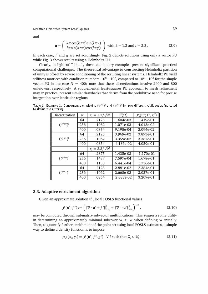
In each case, f and g are set accordingly. Fig. 2 depicts solutions using only a vector PU

while Fig. 3 shows results using a Helmholtz PU.

Clearly, in light of Table 1, these elementary examples present significant practical

computational challenges. The theoretical advantage to constructing Helmholtz partition

of unity is off-set by severe conditioning of the resulting linear systems. Helmholtz PU yield

stiffness matrices with condition numbers 106−107, compared to 102−103 for the simple

vector PU in the case N = 400; note that these discretizations involve 2400 and 800

unknowns, respectively. A supplemental least-squares PU approach to mesh refinement

may, in practice, present similar drawbacks that derive from the prohibitive need for precise

integration over lenticular regions.Table 1: Example 1: Convergen e employing (V h,0)2 and (V h,1)2 for two dierent radii, set as indi atedto dene the overing.Discretization N ri = 1.7/

pN L2(Ω) Jn(u

h; f h, gh)

64 .2125 1.604e-03 1.419e-01

(V h,0)2 256 .1062 1.071e-03 4.013e-02

400 .0854 9.198e-04 2.094e-02

64 .2125 3.969e-02 3.893e-01

(V h,1)2 256 .1062 3.359e-02 3.387e-01

400 .0854 4.186e-02 4.059e-01

ri = 2.3/p

N

64 .2875 1.435e-03 1.170e-01

(V h,0)2 256 .1437 7.597e-04 1.678e-01

400 .1150 6.441e-04 1.736e-01

64 .2125 2.881e-02 2.384e-01

(V h,1)2 256 .1062 2.668e-02 3.037e-01

400 .0854 2.688e-02 3.209e-01

3.3. Adaptive enrichment algorithm

Given an approximate solution uh, local FOSLS functional values

Ji(uh; f h) :=

‖∇ · uh+ f h‖20,Ωi+ ‖∇⊥ · uh‖2

0,Ωi

1/2

. (3.10)

may be computed through submatrix-subvector multiplications. This suggests some utility

in determining an approximately minimal subcover C0 ⊂ C when defining C initially.

Then, to quantify further enrichment of the point set using local FOSLS estimates, a simple

way to define a density function is to impose

ρuh(x i, yi) = Ji(uh; f h, gh) ∀ i such that Ωi ∈ C0. (3.11)


(a) (b)

(c) (d)

(e) (f)Figure 2: For (a)-(b) Example 1, ( )-(d) Example 2, and (e)-(f) Example 3, the exa t solution is shownin red and the omputed solution is shown in bla k. The ases N = 64 and N = 400 using (V h,0)2 aredepi ted.


(a) (b)

(c) (d)

(e) (f)Figure 3: For (a)-(b) Example 1, ( )-(d) Example 2, and (e)-(f) Example 3, the exa t solution is shownin red and the omputed solution is shown in bla k. The ases N = 64 and N = 400 using (V h,1)2 aredepi ted.


Figure 4: Among the interior lo al FOSLS fun tional values, the largest quintile are depi ted in redfor ea h of the three examples. The remainder, in blue, are above the average lo al FOSLS fun tionalvalue.Provided convergence can be improved in practice, this suggests the following simplistic

algorithm for meshfree enrichment:

1. Select an initially-coarse point set and covering to construct a Helmholtz partition

of unity V h,q.

2. Compute uh by solving (3.6).

3. Evaluate local estimates (3.10) ∀ i ∈ C0, as visualized in Fig. 4.

4. Define a density function ρuh(x , y) satisfying (3.11) and assess equi-distribution

of error.

5. If needed, supplement the initial point set in targeted patches subject to ρuh(x , y)

and repeat.

4. Concluding remarks

Given the compromises in efficiency that accompany a truly meshfree approach, its

primary appeal may be as a conformal supplement to more-standard discretizations. In

principle, this could be done precisely within a least-squares setting, whether the mesh-

free flexibility is utilized to resolve multiscale phenomena or to optimize least-squares

approaches to local mesh adaptation [9]. Integration, however, and its impact on condi-

tioning, remains a concern.

Beyond mechanics and classical PDE systems, application of PU methods to dynamic

cell-centered biological simulations may hold special promise [10,11]. This is due to nat-

ural interest in either moving (cell migration), eliminating (cell death), or adding (cell

division) subsets of points used to build multilevel — with respect to biological organiza-

tion — descriptions of various molecular factors and their impact on cell proliferation, cell

differentiation, and cell death in tissue.


Acknowledgments This research is was partially supported by Florida State University

Research Foundation and by Clemson University, under NSF/EPSCoR grant 29-201-xxxx-

0975-223-2094887.

References

[1] S. LI AND W. K. LIU, Meshfree and particle methods and their applications, Appl. Mech. Rev., 55

(2002), pp. 1–34.

[2] T.-P. FRIES AND H. G. MATTHIES, Classification and Overview of Meshfree Methods, Technical

Report, Institure of Scientific Computing, Technical University Braunschweig, 2003.

[3] Q. DU, M. GUNZBURGER, AND L. JU, Meshfree, probabilistic determination of point sets and

support regions for meshless computing, Comput. Meth. Appl. Mech. Eng., 191 (2002), pp.

1349–1366.

[4] M. BERNDT, T. A. MANTEUFFEL, AND S. F. MCCORMICK, Analysis of first-order system least squares

(FOSLS) for elliptic problems with discontinuous coefficients: Part I, SIAM J. Numer. Anal., 43

(2006), pp. 386–408.

[5] X. K. ZHANG, K.-C. KWON, AND S.-K. YOUN, The least-squares meshfree method for the steady

incompressible viscous flow, J. Comput. Phys., 206 (2005), pp. 182–207.

[6] C. A. DUARTE AND J. T. ODEN, H-p Clouds – an h-p meshless method, Numer. Meth. PDEs, 12

(1996), pp. 673–705.

[7] I. BABUSKA AND J. M. MELENK, The partition of unity method, Comput. Meth. Appl. Mech. Eng.,

40 (1997), pp. 727–758.

[8] A. STROUD AND D. SECREST, Gaussian Quadrature Formulas, Prentice Hall, 1966.

[9] P. BOCHEV, G. LIAO, AND G. PENA, Analysis and computation of adaptive moving grids by defor-

mation, Numer. Meth. PDEs, 12 (1996), pp. 489–506.

[10] B. P. AYATI, G. F. WEBB, AND A. R. A. ANDERSON, Computational methods and results for struc-

tured multiscale models of tumor invasion, SIAM Multiscale Model. Simul., 5 (2006), pp. 1–20.

[11] H. R. MACMILLAN, On the potential for explanatory modeling of cellular decisions during neuro-

genesis, Bull. Math. Bio., to appear.

Meshfree First-order System Least...

Documents

Transcript of Meshfree First-order System Least...