MATH 590: Meshfree Methodsfass/590/notes/Notes590_Ch17Print.pdfMATH 590: Meshfree Methods Machine...

MATH 590: Meshfree MethodsMachine Learning

Greg Fasshauer

Department of Applied MathematicsIllinois Institute of Technology

Fall 2014

[email protected] MATH 590 1

http://math.iit.edu/~fass

Outline

1 Introduction

2 Radial Basis Function Networks

3 Classification with Support Vector Machines — Theory

4 Classification with Support Vector Machines — Practice

5 Support Vector Regression



Introduction

Until now

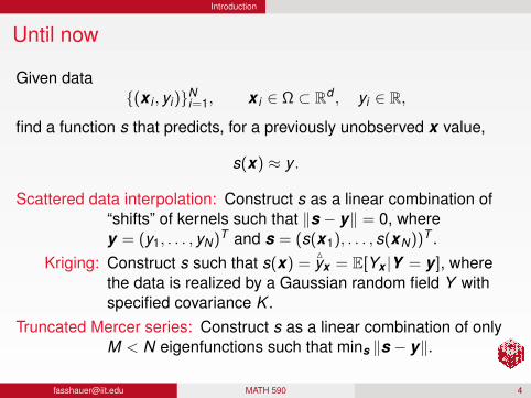
Given data(x i , yi)Ni=1, x i ∈ Ω ⊂ Rd , yi ∈ R,

find a function s that predicts, for a previously unobserved x value,

s(x) ≈ y .

Scattered data interpolation: Construct s as a linear combination of“shifts” of kernels such that ‖s − y‖ = 0, wherey = (y1, . . . , yN)T and s = (s(x1), . . . , s(xN))T .

Kriging: Construct s such that s(x) =Myx = E[Yx |Y = y ], where

the data is realized by a Gaussian random field Y withspecified covariance K .

Truncated Mercer series: Construct s as a linear combination of onlyM < N eigenfunctions such that mins ‖s − y‖.



Introduction

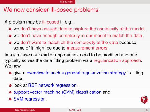
We now consider ill-posed problems

A problem may be ill-posed if, e.g.,we don’t have enough data to capture the complexity of the model,we don’t have enough complexity in our model to match the data,we don’t want to match all the complexity of the data becausesome of it might be due to measurement errors.

In such cases our earlier approaches need to be modified and onetypically solves the data fitting problem via a regularization approach.We now

give a overview to such a general regularization strategy to fittingdata,look at RBF network regression,support vector machine (SVM) classification andSVM regression.



Introduction

Each of our algorithms will involve its own particularloss functioncoupled with an appropriate regularization term with the help of aregularization parameter µ > 0.

The discussion below is quite brief.

Many more details can be found in specialized books or survey paperson machine learning or statistical learning such as, e.g.,[EPP00, HTF09, RW06, SS02, STC04, SC08].



Introduction

Loss function

A typical loss function L depends onan input measurement x ,its associated value yand a value s(x) predicted by the learning algorithm.

The goal of the training phase of the machine learning algorithm is todetermine the predictor s such that the empirical risk

RL =1N

N∑i=1

L (yi , s(x i))

is minimized.



Introduction

Regularization

The regularization functional frequently measures the smoothness ofthe predictor of s.

RemarkThe regularization term can also be interpreted as a measure of thecomplexity of the model (think of an eigenfunction expansion of asmooth function s with rapidly decaying eigenvalues so thathigh-frequency eigenfunctions contribute very little to s, i.e., s is notvery complex).

Example

The quadratic loss L (y ,s) = ‖y − s‖2 coupled with a quadraticregularization functional leads to spline smoothing or penalized leastsquares.This is also what we use for learning via RBF networks.



Introduction

Regularization Theory in RKHSs

If HK (Ω) is a RPHS with reproducing kernel K we can consider cT Kc,the square of the native space norm of s, as the associatedregularization term.

Theorem (Representer Theorem [KW71])

The optimal predictor s in HK (Ω) characterized by

minc

[L (y ,Kc) + µcT Kc

],

can be expressed as a linear combination of kernel functions, i.e.,

s(x) =N∑

j=1

cjK (x ,x j).

Here K is our usual kernel matrix and y = (y1, . . . , yN)T .



Introduction

RemarkFor general L the optimal predictor characterized in therepresenter theorem requires the solution of a non-trivial nonlinearoptimization problem.If L is squared loss and we have a square system matrix K thenthe optimal solution is obtained by simply solving the linearsystem Kc = y , i.e., the empirical risk is zero and the native spacenorm of s is automatically minimized (see also [Fas07,Chapter 19], or the discussion below).



Introduction

RemarkQuestion: Why are we willing to solve an optimization problem

rather than a simple interpolation/regression problem?

Answer: Machine learning applications generally deal with datacontaminated by significant errors (perhaps on the orderof 10% error). This often means that the observed datalook rough, as though generated by a nonsmoothfunction.

A common assumption is that the data were generated by a smoothfunction, but that the observations were corrupted by a nonsmootherror term.



Introduction

RemarkThis suggests we should use smooth basis functions for theapproximation, but should also do some balancing to avoid fitting thenonsmooth errors.

Choosing µ > 0 forces c to not grow too large (and so preventsthe wild oscillations which would be needed to exactly fit data froma nonsmooth function).

A larger µ will demand smaller ci values and care less about fittingthe data.A smaller µ will more closely fit the observed data at the cost of anapproximation which is more susceptible to errors in theobservations, i.e., overfitting.



Radial Basis Function Networks

Machine learning networks follow a supervised learning strategyaccording to which the algorithm learns patterns that exist in a givenset of inputs/outputs (x i , yi)Ni=1.

In its simplest form, the pattern is approximated by a linearcombination of basis functions.

Common choices of basis functions include the Gaussian,trigonometric functions and sigmoids, which have an “on/off” behaviorand are used to reflect the behavior of neurons in a human brain[HTF09, Orr96].

We will consider only so-called single layer learning algorithms usingshifts of the Gaussian kernel (often called the RBF-kernel in thelearning literature).




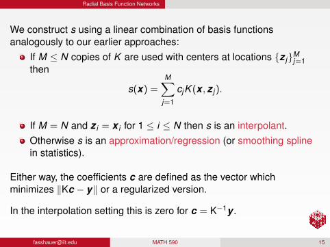
We construct s using a linear combination of basis functionsanalogously to our earlier approaches:

If M ≤ N copies of K are used with centers at locations z jMj=1then

s(x) =M∑

j=1

cjK (x , z j).

If M = N and z i = x i for 1 ≤ i ≤ N then s is an interpolant.Otherwise s is an approximation/regression (or smoothing splinein statistics).

Either way, the coefficients c are defined as the vector whichminimizes ‖Kc − y‖ or a regularized version.

In the interpolation setting this is zero for c = K−1y .




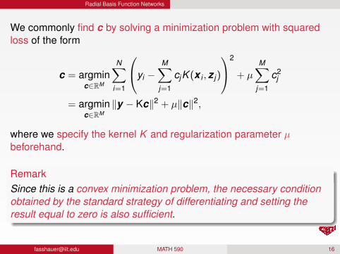
We commonly find c by solving a minimization problem with squaredloss of the form

c = argminc∈RM

N∑i=1

yi −M∑

j=1

cjK (x i , z j)

2

+ µ

M∑j=1

c2j

= argminc∈RM

‖y − Kc‖2 + µ‖c‖2,

where we specify the kernel K and regularization parameter µbeforehand.

RemarkSince this is a convex minimization problem, the necessary conditionobtained by the standard strategy of differentiating and setting theresult equal to zero is also sufficient.




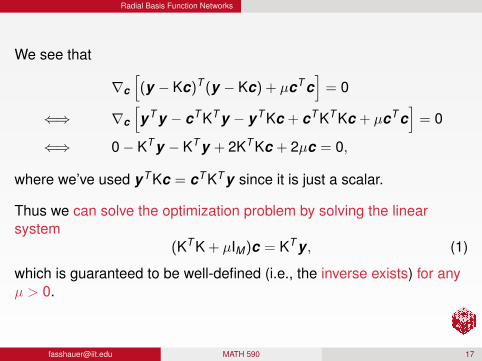
We see that

∇c

[(y − Kc)T (y − Kc) + µcT c

]= 0

⇐⇒ ∇c

[yT y − cT KT y − yT Kc + cT KT Kc + µcT c

]= 0

⇐⇒ 0− KT y − KT y + 2KT Kc + 2µc = 0,

where we’ve used yT Kc = cT KT y since it is just a scalar.

Thus we can solve the optimization problem by solving the linearsystem

(KT K + µIM)c = KT y , (1)

which is guaranteed to be well-defined (i.e., the inverse exists) for anyµ > 0.




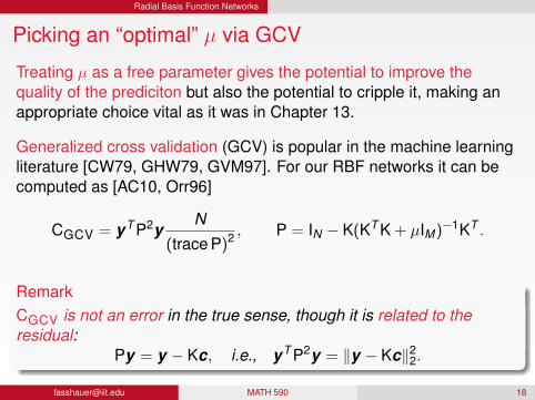
Picking an “optimal” µ via GCV

Treating µ as a free parameter gives the potential to improve thequality of the prediciton but also the potential to cripple it, making anappropriate choice vital as it was in Chapter 13.

Generalized cross validation (GCV) is popular in the machine learningliterature [CW79, GHW79, GVM97]. For our RBF networks it can becomputed as [AC10, Orr96]

CGCV = yT P2yN

(trace P)2 , P = IN − K(KT K + µIM)−1KT .

RemarkCGCV is not an error in the true sense, though it is related to theresidual:

Py = y − Kc, i.e., yT P2y = ‖y − Kc‖22.



Radial Basis Function Networks Numerical experiments for regression with RBF networks

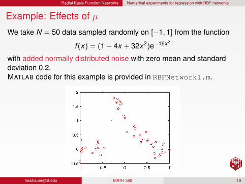
Example: Effects of µ

We take N = 50 data sampled randomly on [−1,1] from the function

f (x) = (1− 4x + 32x2)e−16x2

with added normally distributed noise with zero mean and standarddeviation 0.2.MATLAB code for this example is provided in RBFNetwork1.m.




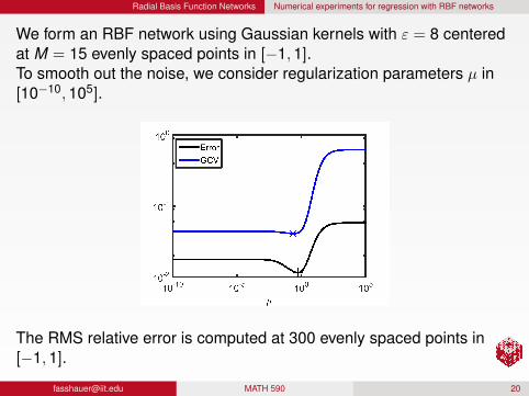
We form an RBF network using Gaussian kernels with ε = 8 centeredat M = 15 evenly spaced points in [−1,1].To smooth out the noise, we consider regularization parameters µ in[10−10,105].

The RMS relative error is computed at 300 evenly spaced points in[−1,1].




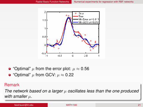
“Optimal” µ from the error plot: µ ≈ 0.56“Optimal” µ from GCV: µ ≈ 0.22

RemarkThe network based on a larger µ oscillates less than the one producedwith smaller µ.




RemarkThe smoothing parameter µ can affect the quality of the predictionin an understandable (larger µ yields less oscillation) butunpredictable (the optimal amount of oscillation is unknown apriori) way, much as the shape parameter ε works in unpredictableways.

Due to the ill-conditioning of KT K as ε→ 0, for small ε values, µmay actually improve the condition of the solution.

There is a complicated relationship between µ and ε. For somekernels µ may improve the accuracy through smoothing out noiseand for others it may improve the quality by reducingill-conditioning.

Although µ affects the quality of the prediction s, it does notchange the native space HK (it pushes the interpolant toward aset of functions which try to minimize ‖c‖2 rather than ‖s‖HK ). Incontrast, changing ε changes K and, therefore, HK .




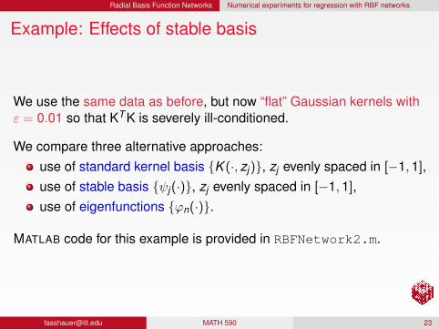
Example: Effects of stable basis

We use the same data as before, but now “flat” Gaussian kernels withε = 0.01 so that KT K is severely ill-conditioned.

We compare three alternative approaches:use of standard kernel basis K (·, zj), zj evenly spaced in [−1,1],use of stable basis ψj(·), zj evenly spaced in [−1,1],use of eigenfunctions ϕn(·).

MATLAB code for this example is provided in RBFNetwork2.m.




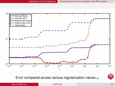
Error compared across various regularization values µ.




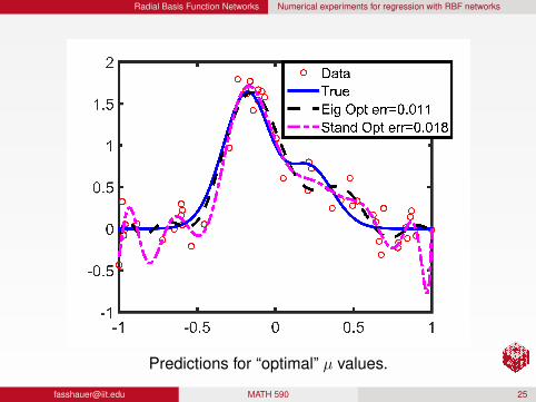
Predictions for “optimal” µ values.




RemarkThe stable basis outperforms the standard basis for most µ values.

Eigenfunctions and the stable basis essentially overlap.

For large µ values, the prediction is dominated by theregularization component (cf. the overlap near µ ≈ 104).

The similarity between the stable basis and eigenfunctions is dueto the fact that the correction term in the HS-SVD decreases inmagnitude as ε decreases.

Even a tiny value of µ has a remarkable stabilization effect in thisexample.




Example: Combined effects of µ and ε

Again, same data as before, but now we look at the effect of allowingboth ε and µ to change.

Only the eigenfunction basis is considered.

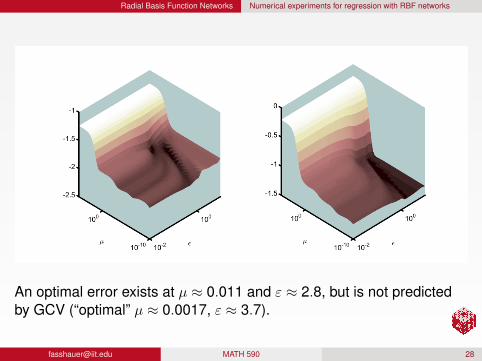
The errors for µ ∈ [10−10,105] and ε ∈ [10−2,101], along with GCVplots are shown below.

MATLAB code for this example is provided in RBFNetwork3.m.




An optimal error exists at µ ≈ 0.011 and ε ≈ 2.8, but is not predictedby GCV (“optimal” µ ≈ 0.0017, ε ≈ 3.7).



Classification with Support Vector Machines — Theory

We now discuss the two main applications of support vector machines(SVMs) in the context of supervised machine learning:

classification andregression.

Both of these applications can be formulated within the regularizationframework outlined at the beginning of this chapter.




Standard (binary) classification

Given: a set of training data (x i , yi) : i = 1, . . . ,N withmeasurements x i ∈ Rd anddata values in the form of labels yi ∈ −1,+1.

Find: a predictor s that will allow us to assign an appropriate label,either −1 or +1, to a future measurement x .




ExampleA predictor might be

s(x) = sign (h(x)) ,

where h denotes a hyperplane separating the given measurements.

A typical loss function is given by the hinge loss (or soft margin loss)

L (y ,h(x)) = max (1− yh(x),0)

sinceL (y ,h(x)) = 0 ⇐⇒ yh(x) ≥ 1,

i.e., y and h(x) have the same sign and |h(x)| ≥ 1 so that we haveenough confidence in our prediction (see, e.g., [SS02, Chapter 3]).

An appropriate regularization term will be given by some norm of h(see below for more details).




Regression

We estimate continuous numeric values as discussed in the previoussection.As for RBF networks, we can use the squared loss

L (y , s(x)) = (y − s(x))2 .

Alternatively, the so-called ε-insensitive loss

L (y , s(x)) = max (|y − s(x)| − ε,0)

is used as a symmetric analogue of the hinge loss.

RemarkAccording to the ε-insensitive loss function, deviations of the predictedvalue s(x) from the correct value y are only penalized if they exceed ε,and therefore it will be possible to obtain sparse representations usingonly a subset of the data referred to as support vectors (more detailsbelow).



Classification with Support Vector Machines — Theory Linear classification

Linear Classification

The simplest predictor is given by

s(x) = sign (h(x)) ,

where h denotes a hyperplane — directly in input space — of the form

h(x) = xT w + b = 0, x ∈ Rd ,

that separates the measurements with label −1 from those with a +1.

The weights w (which serve as the unit normal vector to thehyperplane) and the bias b can be determined by maximizing themargin or gap to both sides of this hyperplane (see, e.g., [HTF09,Chapter 12]).




Unconstrained minimization

Since the size of the margin is 1‖w‖ , and we want to maximize this

margin, a natural regularization functional is:

minimize ‖w‖ (norm of the coefficients of h).

Using the hinge loss function and h(x) = xT w + b, we get theunconstrained minimization problem

minw ,b

[1N

N∑i=1

max (1− yih(x i),0) + µ12

wT w

],

where µ is an appropriately chosen regularization parameter.




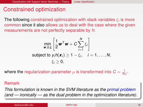
Constrained optimization

The following constrained optimization with slack variables ξi is morecommon since it also allows us to deal with the case where the givenmeasurements are not perfectly separable by h:

minw ,b,ξ

[12

wT w + CN∑

i=1

ξi

]subject to yih(x i) ≥ 1− ξi , i = 1, . . . ,N,

ξi ≥ 0,

where the regularization parameter µ is transformed into C = 1Nµ .

RemarkThis formulation is known in the SVM literature as the primal problem(and — ironically — as the dual problem in the optimization literature).




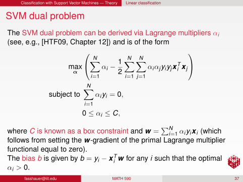
SVM dual problem

The SVM dual problem can be derived via Lagrange multipliers αi(see, e.g., [HTF09, Chapter 12]) and is of the form

maxα

N∑i=1

αi −12

N∑i=1

N∑j=1

αiαjyiyjxTi x j

subject to

N∑i=1

αiyi = 0,

0 ≤ αi ≤ C,

where C is known as a box constraint and w =∑N

i=1 αiyix i (whichfollows from setting the w -gradient of the primal Lagrange multiplierfunctional equal to zero).The bias b is given by b = yi − xT

i w for any i such that the optimalαi > 0.




RemarkFor stability purposes we compute the bias by considering allqualifying indices and find b using the mean.

The box constraint C is a free parameter which needs to be eitherset by the user or determined by an additional parameteroptimization methods such as cross validation.



Classification with Support Vector Machines — Theory Kernel classification

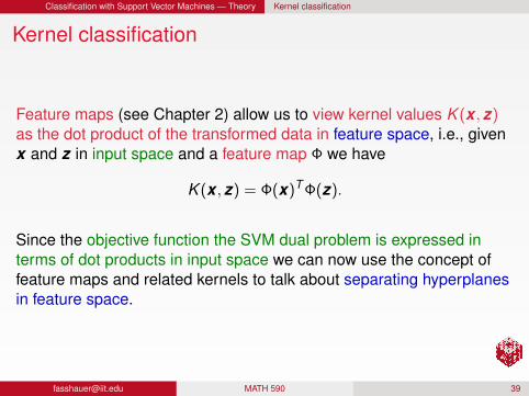
Kernel classification

Feature maps (see Chapter 2) allow us to view kernel values K (x , z)as the dot product of the transformed data in feature space, i.e., givenx and z in input space and a feature map Φ we have

K (x , z) = Φ(x)T Φ(z).

Since the objective function the SVM dual problem is expressed interms of dot products in input space we can now use the concept offeature maps and related kernels to talk about separating hyperplanesin feature space.




RemarkThe feature space is potentially infinite-dimensional (as, e.g., inthe case of the Gaussian kernel) and therefore offers much moreflexibility for separating the data than the finite-dimensional inputspace.

Cover’s theorem [Cov65] provides a theoretical foundation for this.It ensures that data which can not be separated by a hyperplanein input space most likely will be linearly separable after beingtransformed to feature space by a suitable feature map.

Thus, support vector machines — and kernel machines, inparticular — are a good tool to use in order to tackle difficult dataclassification problems.




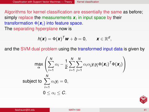
Algorithms for kernel classification are essentially the same as before;simply replace the measurements x i in input space by theirtransformation Φ(x i) into feature space.The separating hyperplane now is

h(x) = Φ(x)T w + b = 0, x ∈ Rd ,

and the SVM dual problem using the transformed input data is given by

maxα

N∑i=1

αi −12

N∑i=1

N∑j=1

αiαjyiyjΦ(x i)T Φ(x j)

subject to

N∑i=1

αiyi = 0,

0 ≤ αi ≤ C.




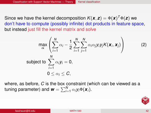
Since we have the kernel decomposition K (x , z) = Φ(x)T Φ(z) wedon’t have to compute (possibly infinite) dot products in feature space,but instead just fill the kernel matrix and solve

maxα

N∑i=1

αi −12

N∑i=1

N∑j=1

αiαjyiyjK (x i ,x j)

(2)

subject toN∑

i=1

αiyi = 0,

0 ≤ αi ≤ C,

where, as before, C is the box constraint (which can be viewed as atuning parameter) and w =

∑Ni=1 αiyiΦ(x i).




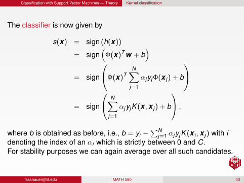
The classifier is now given by

s(x) = sign (h(x))

= sign(

Φ(x)T w + b)

= sign

Φ(x)TN∑

j=1

αjyjΦ(x j) + b

= sign

N∑j=1

αjyjK (x ,x j) + b

,

where b is obtained as before, i.e., b = yi −∑N

j=1 αjyjK (x i ,x j) with idenoting the index of an αi which is strictly between 0 and C.For stability purposes we can again average over all such candidates.




What does the separating hyperplane in this case look like?

The hyperplane will be linear only in feature space (which weusually have no concrete knowledge of). In the input space thedata will be separated by a nonlinear manifold.

The representation of this manifold is sparse in the sense that notall basis functions are needed to specify it.

Only those centers x j whose corresponding αj are nonzero definemeaningful basis functions.These special centers are referred to as support vectors.




RemarkSince the decision boundary can be expressed in terms of alimited number of support vectors, i.e., it has a sparserepresentation, learning is possible in very high-dimensional inputspaces [SC08].

SVMs arerobust against several types of model violations and outliers,computationally efficient, e.g., by using sequential minimaloptimization (SMO) [Pla99] to perform the quadratic optimizationtask required for classification as well as regression.

Another way to make SVMs perform more efficiently is to considera low-rank representation for the kernel [FS02]. Below we test ourown version based on eigenfunctions.




RemarkFor positive definite kernels one can formulate the separatinghyperplane without the bias term b. In that case the equalityconstraint

∑Ni=1 αiyi = 0 (which may be somewhat of a nuisance

during the optimization process) can be omitted [PMR+01].

The primal and dual formulations each have their advantages.The primal formulation (in input space) is good for large amounts ofrather low-dimensional data.The dual formulation (with kernels in feature space) is good forhigh-dimensional data (since only the number of support vectorsmatter).




RemarkIn our numerical experiments we use Gaussian kernels.

Linear SVM uses the dot product kernel K (x , z) = xT z .

Other popular kernels arepolynomial kernels of degree β in the form K (x , z) = (1 + xT z)β ,the sigmoid kernel (or multilayer perceptron)K (x , z) = tanh(1 + εxT z).

Kernels may be defined via the feature map (instead of in closedform), and this feature map can be picked depending on thespecific application (e.g., as a string kernel for text mining).



Classification with Support Vector Machines — Practice Numerical experiments for classification with kernel SVMs

Example: Simple kernel classification

This example is from [HTF09, Section 2.3] (see also help for SVMs inMATLAB’s Statistics Toolbox).

We attempt to learn/classify data coming from two differentpopulations:

population 1, normally distributed with center at (1,0) (filled redcircle) and identity covariancepopulation 2, normally distributed with center at (0,1) (filled greensquare) and identity covariance

Use Gaussian kernels with varying shape parameter ε and boxconstraint C.

MATLAB code for this example is provided in SVM1.m which usesSVM_Setup.m and gqr_fitsvm.m.




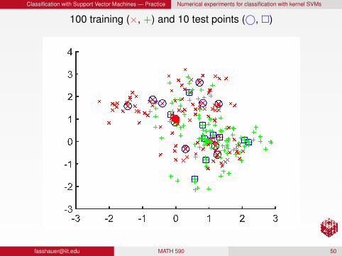
100 training (×, +) and 10 test points (©, )




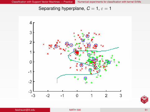
Separating hyperplane, C = 1, ε = 1




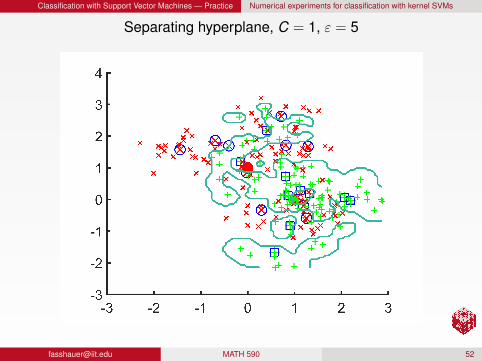
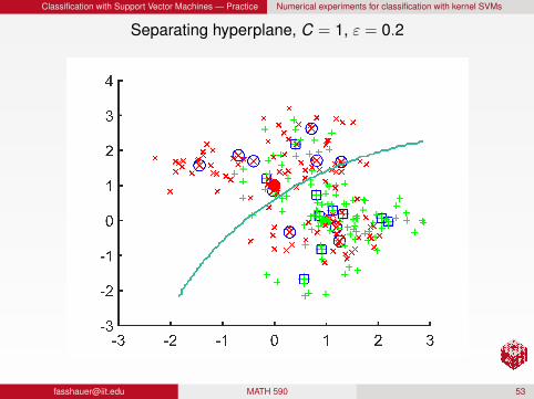
Separating hyperplane, C = 1, ε = 0.2




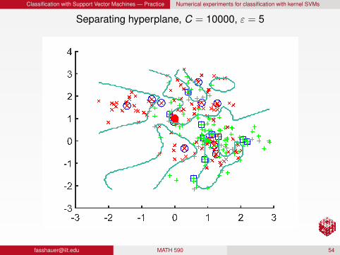
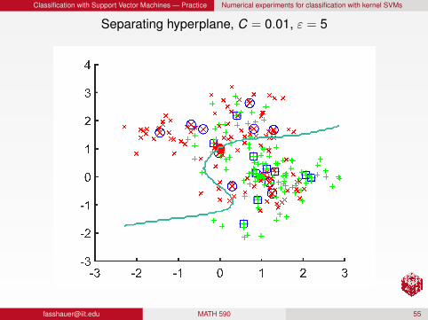
Separating hyperplane, C = 0.01, ε = 5




RemarkFor a fixed C, larger ε produces a more localized/detailedseparatorFor a fixed ε, larger C produces a more localized/detailedseparator




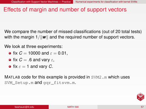
Effects of margin and number of support vectors

We compare the number of missed classifications (out of 20 total tests)with the margin 1/‖w‖ and the required number of support vectors.

We look at three experiments:fix C = 10000 and ε = 0.01,fix C = .6 and vary ε,fix ε = 1 and vary C.

MATLAB code for this example is provided in SVM2.m which usesSVM_Setup.m and gqr_fitsvm.m.




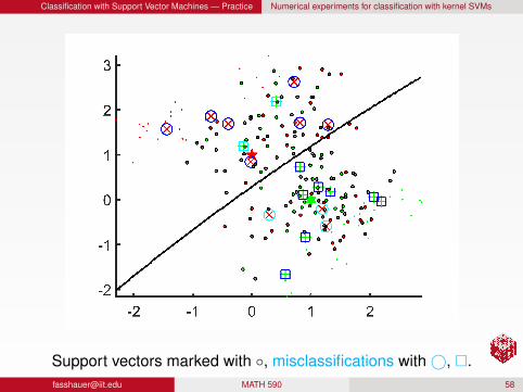
Support vectors marked with , misclassifications with©, [email protected] MATH 590 58



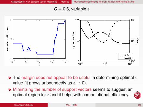
C = 0.6, variable ε

The margin does not appear to be useful in determining optimal εvalue (it grows unboundedly as ε→ 0).Minimizing the number of support vectors seems to suggest anoptimal region for ε and it helps with computational efficiency.




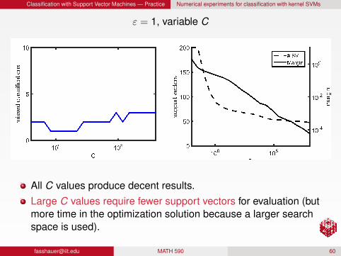
ε = 1, variable C

All C values produce decent results.Large C values require fewer support vectors for evaluation (butmore time in the optimization solution because a larger searchspace is used).




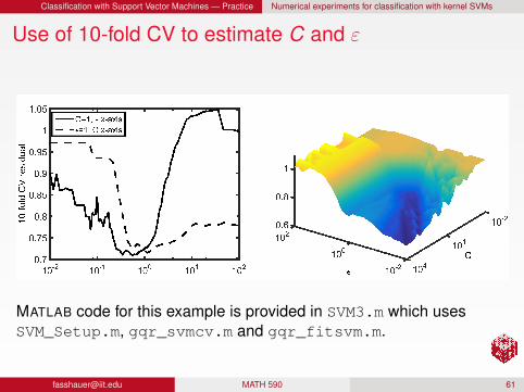
Use of 10-fold CV to estimate C and ε

MATLAB code for this example is provided in SVM3.m which usesSVM_Setup.m, gqr_svmcv.m and gqr_fitsvm.m.




RemarkThe example just discussed uses a linearly separable pattern since thepopulation centers (0,1) and (1,0) are linearly separable.

Because the ε→ 0 limit of Gaussians is a polynomial, it is reasonableto conclude that, with infinitely much data drawn from thosepopulations, the optimal SVM would have ε→ 0 to produce a line.

We therefore next consider a different pattern which is not linearlyseparable.




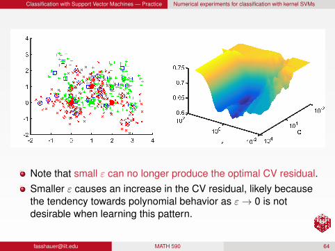
Pattern that is not linearly separable

We want to classify data as coming from one of two populations:population 1 (denoted by© and ×) with centers at(0,0), (1,1), (2,0) (filled©), andpopulation 2 (denoted by and +), with centers at(0,1), (1,0), (2,1) (filled ).

Test points (large ×, +) and training points (small ×, +) are shown inthe figure.

MATLAB code for this example is provided in SVM4.m which usesSVM_Setup.m, gqr_svmcv.m and gqr_fitsvm.m.




Note that small ε can no longer produce the optimal CV residual.Smaller ε causes an increase in the CV residual, likely becausethe tendency towards polynomial behavior as ε→ 0 is notdesirable when learning this pattern.



Classification with Support Vector Machines — Practice Computational consideration for classification with kernel SVMs

Computational consideration for classification withkernel SVMs

SVMs are generally more popular than RBF networks.On the one hand, SVMs may require many fewer kernel centersfor evaluation, i.e., they have a spare representation (only thenonzero coefficients must be included).However, solving the quadratic program (2) is more expensivethan solving the linear system (1).

We nowlook at that cost as a function of ε and C, andpresent a strategy for exploiting the low rank eigenfunctionrepresentation for small ε to decrease cost.




RemarkWe use the quadprog solver with the algorithminterior-point-convex from MATLAB’s Optimization Toolboxwith initial guess C/2 times a vector of ones.

As always for iterative solvers, a good initial guess helps speed upconvergence.




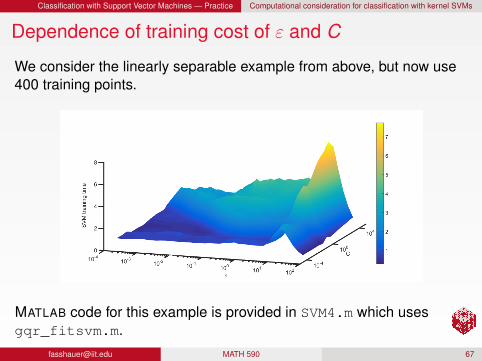
Dependence of training cost of ε and C

We consider the linearly separable example from above, but now use400 training points.

MATLAB code for this example is provided in SVM4.m which usesgqr_fitsvm.m.




RemarkThe solution time for the quadratic program clearly depends on ε andC.

Very large ε and very small C seem to be solved quickly:large ε because the alertkernel is very localized,and small C because the solution domain is very small and quicklysearched.

Larger values of C seem to always take longer, likely because thesearch space is increasing.




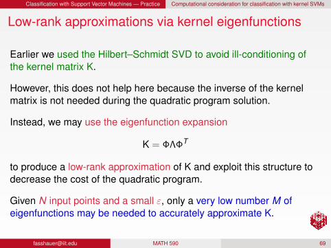
Low-rank approximations via kernel eigenfunctions

Earlier we used the Hilbert–Schmidt SVD to avoid ill-conditioning ofthe kernel matrix K.

However, this does not help here because the inverse of the kernelmatrix is not needed during the quadratic program solution.

Instead, we may use the eigenfunction expansion

K = ΦΛΦT

to produce a low-rank approximation of K and exploit this structure todecrease the cost of the quadratic program.

Given N input points and a small ε, only a very low number M ofeigenfunctions may be needed to accurately approximate K.




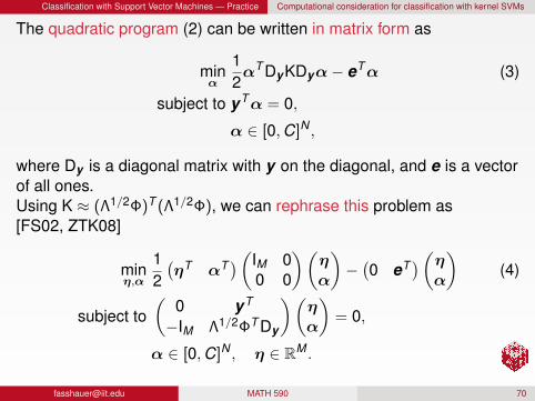
The quadratic program (2) can be written in matrix form as

minα

12αT DyKDyα− eTα (3)

subject to yTα = 0,

α ∈ [0,C]N ,

where Dy is a diagonal matrix with y on the diagonal, and e is a vectorof all ones.Using K ≈ (Λ1/2Φ)T (Λ1/2Φ), we can rephrase this problem as[FS02, ZTK08]

minη,α

12(ηT αT

)(IM 00 0

)(ηα

)−(0 eT

)(ηα

)(4)

subject to(

0 yT

−IM Λ1/2ΦT Dy

)(ηα

)= 0,

α ∈ [0,C]N , η ∈ RM .




RemarkAlthough this system is of size N + M (and the original system wasonly size N), the cost of solving this system may be much lowerbecause of the extremely simple structure of the Hessian.

This sparsity, in comparison to H which may be fully dense, allows forcheap matrix-vector products and decompositions, both of which mayall for a faster quadratic program solve.

Note that the η values are inconsequential in making predictions withthe SVM.




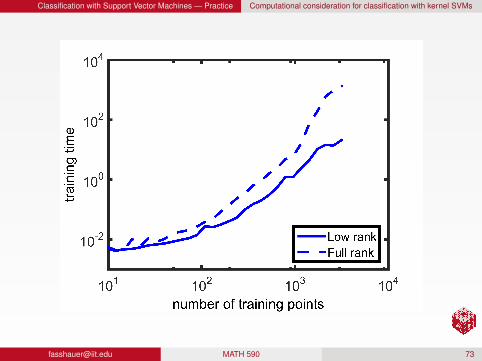
Low-rank vs. full-rank approximation

We use the same setup as before (given in SVM5.m).

We study the cost of solving the quadratic program and training theSVM. Minimizing this cost is an important topic in machine learning(see, e.g., [YDD04, FL02, LLZ+11]).

Increasingly large sets of input points are considered and the cost ofsolving the full rank problem (3) is compared to solving the low rankproblem (4).

The kernel is parameterized with ε = .01 and C = 1 and theeigenfunctions of the Gaussian use α = 106.



Support Vector Regression Linear support vector regression

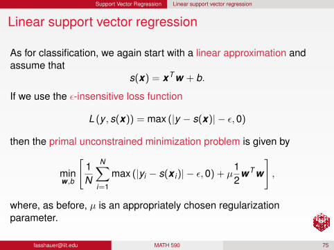
Linear support vector regression

As for classification, we again start with a linear approximation andassume that

s(x) = xT w + b.

If we use the ε-insensitive loss function

L (y , s(x)) = max (|y − s(x)| − ε,0)

then the primal unconstrained minimization problem is given by

minw ,b

[1N

N∑i=1

max (|yi − s(x i)| − ε,0) + µ12

wT w

],

where, as before, µ is an appropriately chosen regularizationparameter.




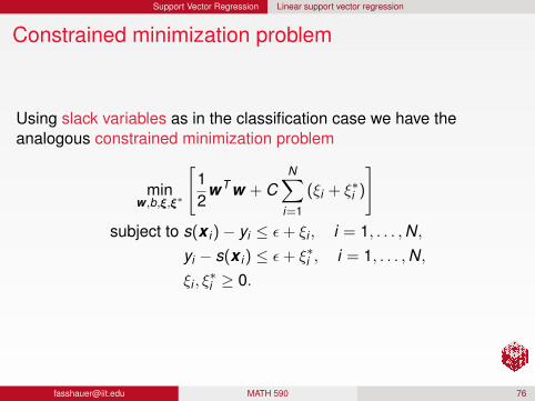
Constrained minimization problem

Using slack variables as in the classification case we have theanalogous constrained minimization problem

minw ,b,ξ,ξ∗

[12

wT w + CN∑

i=1

(ξi + ξ∗i )

]subject to s(x i)− yi ≤ ε+ ξi , i = 1, . . . ,N,

yi − s(x i) ≤ ε+ ξ∗i , i = 1, . . . ,N,ξi , ξ

∗i ≥ 0.




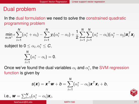
Dual problem

In the dual formulation we need to solve the constrained quadraticprogramming problem

minα,α∗

ε

N∑i=1

(α∗i + αi)−N∑

i=1

yi(α∗i − αi) +

12

N∑i=1

N∑j=1

(α∗i − αi)(α∗j − αj)xTi x j

subject to 0 ≤ αi , α∗i ≤ C,

N∑i=1

(α∗i − αi) = 0.

Once we’ve found the dual variables αi and α∗i , the SVM regressionfunction is given by

s(x) = xT w + b =N∑

i=1

(α∗i − αi)xT x i + b,

i.e., w =∑N

i=1(α∗i − αi)x i [email protected] MATH 590 77



RemarkThe computation of the bias term b follows from the KKTconditions (for details see [SS02]) and is similar in spirit to theclassification setting, i.e.,

b = yi − xTi w − ε for αi ∈ (0,C),

b = yi − xTi w + ε for α∗i ∈ (0,C).

As before, any one of these will theoretically suffice, but forstability reasons it is better to compute b via an average over allcandidates.

As in the classification setting, α∗i −αi 6= 0 only for some i, and thecorresponding measurements x i are called the support vectors.

For more details see, e.g., [HTF09, Chapter 12], [SS02,Chapter 9].



Support Vector Regression Nonlinear support vector regression

Nonlinear support vector regression

As for classification, we obtain a nonlinear “kernelized” regression fit ifwe map the data into feature space and then use kernels.

This is straightforward and completely analogous to the classificationsetting.




The resulting dual problem is

minα,α∗

ε

N∑i=1

(α∗i + αi )−

N∑i=1

yi (α∗i − αi ) +

12

N∑i=1

N∑j=1

(α∗i − αi )(α∗

j − αj )K (x i ,x j )

subject to 0 ≤ αi , α∗i ≤ C,

N∑i=1

(α∗i − αi ) = 0,

so that

s(x) = Φ(xT )w + b =N∑

i=1

(α∗i − αi )K (x ,x i ) + b,

i.e., w =∑N

i=1(α∗i − αi )Φ(x i ) and

b = yi −N∑

j=1

(α∗j − αj )K (x i ,x j )− ε for αi ∈ (0,C),

b = yi −N∑

j=1

(α∗j − αj )K (x i ,x j ) + ε for α∗

i ∈ (0,C).




RemarkMany more details on all aspects of machine learning can be found,e.g., in the

books [Alp09, HTF09, RW06, SS02, STC04, SC08] orsurvey papers [EPP00, MMn06, Orr96].



Appendix References

References I

[AC10] S. Arlot and A. Celisse, A survey of cross-validation procedures for modelselection, Statistics surveys 4 (2010), 40–79.

[Alp09] Ethem Alpaydin, Introduction to Machine Learning, 2nd ed., The MITPress, December 2009.

[Cov65] Thomas M. Cover, Geometrical and statistical properties of systems oflinear inequalities with applications in pattern recognition, IEEETransactions on Electronic Computers 14 (1965), 326–334.

[CW79] Peter Craven and Grace Wahba, Smoothing noisy data with splinefunctions, Numerische Mathematik 31 (1979), no. 4, 377–403.

[EPP00] Theodoros Evgeniou, Massimiliano Pontil, and Tomaso Poggio,Regularization networks and support vector machines, Advances inComputational Mathematics 13 (2000), no. 1, 1–50.

[Fas07] G. E. Fasshauer, Meshfree Approximation Methods with MATLAB,Interdisciplinary Mathematical Sciences, vol. 6, World Scientific PublishingCo., Singapore, 2007.



Appendix References

References II

[FL02] G. W. Flake and S. Lawrence, Efficient SVM regression training with SMO,Machine Learning 46 (2002), no. 1-3, 271–290.

[FS02] Shai Fine and Katya Scheinberg, Efficient SVM training using low-rankkernel representations, J. Mach. Learn. Res. 2 (2002), 243–264.

[GHW79] G. H. Golub, M. Heath, and G. Wahba, Generalized cross-validation as amethod for choosing a good ridge parameter, Technometrics 21 (1979),no. 2, 215–223.

[GVM97] G. H. Golub and U. Von Matt, Generalized cross-validation for large-scaleproblems, Journal of Computational and Graphical Statistics 6 (1997),no. 1, 1–34.

[HTF09] T. Hastie, R. Tibshirani, and J. Friedman, Elements of Statistical Learning:Data Mining, Inference, and Prediction, 2nd ed., Springer Series inStatistics, Springer, New York, 2009.

[KW71] G. Kimeldorf and G. Wahba, Some results on Tchebycheffian splinefunctions, J. Math. Anal. Applic. 33 (1971), 82–95.



Appendix References

References III

[LLZ+11] Y. Lin, F. Lv, S. Zhu, M. Yang, T. Cour, K. Yu, L. Cao, and T. Huang,Large-scale image classification: fast feature extraction and SVM training,2011 IEEE Conference on Computer Vision and Pattern Recognition(CVPR), IEEE, 2011, pp. 1689–1696.

[MMn06] Javier M. Moguerza and Alberto Muñoz, Support vector machines withapplications, Statistical Science 21 (2006), no. 3, 322–336.

[Orr96] M. J. L. Orr, Introduction to radial basis function networks, Tech. report,University of Edinburgh, Centre for Cognitive Sciences, 1996.

[Pla99] John C. Platt, Fast training of support vector machines using sequentialminimal optimization, Advances in Kernel Methods (Bernhard Schölkopf,Christopher J. C. Burges, and Alexander J. Smola, eds.), MIT Press,Cambridge, MA, USA, 1999, pp. 185–208.

[PMR+01] T. Poggio, S. Mukherjee, R. Rifkin, A. Rakhlin, and A. Verri, b, Tech. report,MIT AI Memo 2001-011, 2001.



Appendix References

References IV

[RW06] C. E. Rasmussen and C. Williams, Gaussian Processes for MachineLearning, MIT Press, Cambridge, Massachussetts, 2006.

[SC08] I. Steinwart and A. Christmann, Support Vector Machines, InformationScience and Statistics, Springer, New York, 2008.

[SS02] B. Schölkopf and A. J. Smola, Learning with Kernels: Support VectorMachines, Regularization, Optimization, and Beyond, The MIT Press,2002.

[STC04] J. Shawe-Taylor and N. Cristianini, Kernel Methods for Pattern Analysis,Cambridge University Press, 2004.

[YDD04] C. Yang, R. Duraiswami, and L. S. Davis, Efficient kernel machines usingthe improved fast Gauss transform, Advances in neural informationprocessing systems, 2004, pp. 1561–1568.

[ZTK08] K. Zhang, I. W Tsang, and J. T Kwok, Improved Nyström low-rankapproximation and error analysis, Proceedings of the 25th internationalconference on Machine learning, ACM, 2008, pp. 1232–1239.



MATH 590: Meshfree Methodsfass/590/notes/Notes590_Ch17Print.pdfMATH 590: Meshfree Methods Machine...

Documents

Transcript of MATH 590: Meshfree Methodsfass/590/notes/Notes590_Ch17Print.pdfMATH 590: Meshfree Methods Machine...