Mesh management methods in finite element simulations of orthodontic...
33
This is a repository copy of Mesh management methods in finite element simulations of orthodontic tooth movement. White Rose Research Online URL for this paper: http://eprints.whiterose.ac.uk/92644/ Version: Accepted Version Article: Mengoni, M, Ponthot, JP and Boman, R (2016) Mesh management methods in finite element simulations of orthodontic tooth movement. Medical Engineering and Physics, 38 (2). pp. 140-147. ISSN 1350-4533 https://doi.org/10.1016/j.medengphy.2015.11.005 © 2015. This manuscript version is made available under the CC-BY-NC-ND 4.0 license http://creativecommons.org/licenses/by-nc-nd/4.0/ [email protected] https://eprints.whiterose.ac.uk/ Reuse Unless indicated otherwise, fulltext items are protected by copyright with all rights reserved. The copyright exception in section 29 of the Copyright, Designs and Patents Act 1988 allows the making of a single copy solely for the purpose of non-commercial research or private study within the limits of fair dealing. The publisher or other rights-holder may allow further reproduction and re-use of this version - refer to the White Rose Research Online record for this item. Where records identify the publisher as the copyright holder, users can verify any specific terms of use on the publisher’s website. Takedown If you consider content in White Rose Research Online to be in breach of UK law, please notify us by emailing [email protected] including the URL of the record and the reason for the withdrawal request.
Transcript of Mesh management methods in finite element simulations of orthodontic...
This is a repository copy of Mesh management methods in finite element simulations of orthodontic tooth movement.
White Rose Research Online URL for this paper:http://eprints.whiterose.ac.uk/92644/
Version: Accepted Version
Article:
Mengoni, M, Ponthot, JP and Boman, R (2016) Mesh management methods in finite element simulations of orthodontic tooth movement. Medical Engineering and Physics, 38 (2). pp. 140-147. ISSN 1350-4533
https://doi.org/10.1016/j.medengphy.2015.11.005
© 2015. This manuscript version is made available under the CC-BY-NC-ND 4.0 license http://creativecommons.org/licenses/by-nc-nd/4.0/
[email protected]://eprints.whiterose.ac.uk/
Reuse
Unless indicated otherwise, fulltext items are protected by copyright with all rights reserved. The copyright exception in section 29 of the Copyright, Designs and Patents Act 1988 allows the making of a single copy solely for the purpose of non-commercial research or private study within the limits of fair dealing. The publisher or other rights-holder may allow further reproduction and re-use of this version - refer to the White Rose Research Online record for this item. Where records identify the publisher as the copyright holder, users can verify any specific terms of use on the publisher’s website.
Takedown
If you consider content in White Rose Research Online to be in breach of UK law, please notify us by emailing [email protected] including the URL of the record and the reason for the withdrawal request.
Mesh Management Methods in Finite Element
Simulations of Orthodontic Tooth Movement
M. Mengonia,∗, J.P. Ponthota, R. Bomana
aUniversity of Liege (ULg), Department of Aerospace and Mechanical Engineering,Non-linear Computational Mechanics (LTAS/MN2L), Liege, Belgium
Abstract
In finite element simulations of orthodontic tooth movement, one of the chal-
lenges is to represent long term tooth movement. Large deformation of the
periodontal ligament and large tooth displacment due to bone remodelling
lead to large distortions of the finite element mesh when a Lagrangian for-
malism is used. We propose in this work to use an Arbitrary Lagrangian
Eulerian (ALE) formalism to delay remeshing operations. A large tooth dis-
placement is obtained including effect of remodelling without the need of
remeshing steps but keeping a good-quality mesh. Very large deformations
in soft tissues such as the periodontal ligament is obtained using a combi-
nation of the ALE formalism used continuously and a remeshing algorithm
used when needed. This work demonstrates that the ALE formalism is a
very efficient way to delay remeshing operations.
Keywords: Orthodontic Tooth Movement, Arbitrary Lagrangian Eulerian
formalism, Remeshing, Finite Element Method
Word count: 3706
∗Corresponding author.Email address: [email protected] (M. Mengoni)
Preprint submitted to Medical Engineering & Physics September 10, 2015
1. Introduction1
The Finite Element (FE) Method is a numerical procedure to approx-2
imate problems modelled by partial differential equations using a discrete3
representation of the problem to be solved on a grid of nodes and elements.4
In mechanical models, it involves procedures to calculate in each element5
stresses and strains resulting from external factors such as forces and dis-6
placements. The FE method is extremely useful for estimating mechanical7
response of biomaterials and tissues that can hardly be measured in vivo.8
It has been used in dentistry-related problems since the 1970’s, as reviewed9
in [1, 2, 3], with the interest of determining stresses in dental structures and10
materials used for clinical treatment and repair, and to improve the strength11
and response of these treatments, procedures and associated adaptive be-12
haviour of the tissues. In particular, for orthodontic tooth movement prob-13
lems, the FE method can deliver not only the global mechanical behaviour14
of the involved structures, i.e. the tooth mobility, but also it gives access to15
local stresses and strains of each tissue. That local behaviour is essential to16
couple mechanics and biology and to model the adaptive response of tissues.17
One of the main principles of orthodontic treatment is to impose external18
loads to a tooth, leading to an altered mechanical environment in the peri-19
odontal ligament (PDL) surrounding the tooth and bone tissues supporting20
it. This altered environment induces remodelling and leads the tooth into a21
new position. The driving force of remodelling is the biological interaction22
between bone tissues and the PDL. Remodelling models in orthodontics FE23
analysis usually involve an update of the purely mechanical displacement of24
the tooth due to applied forces by a displacement due to the remodelling25
2
stimulus [4, 5]. The stimulus for remodelling is either the strain energy den-26
sity [6], based on the strain field [7, 8, 9], or based on the stress field [10].27
However, other approaches can also be found: Soncini and Pietrabissa [11]28
or van Schepdael et al. [12] proposed remodelling models considering a vis-29
cous behaviour of the bone (viscoelastic Maxwell models) ; Cronau et al. [13]30
proposed a remodelling model considering a viscous behaviour of the PDL31
(viscoelastic Maxwell model) ; finally, Field et al. [14], Lin et al. [15], Men-32
goni and Ponthot [16] proposed remodelling laws involving an explicit local33
change of the bone elastic properties based on the strain level, similarly to34
remodelling algorithms used within the orthopaedic biomechanics literature.35
In any case, due to remodelling and therefore softening of the bone tissue,36
or when the PDL deformations are physically modelled, large deformations37
are locally encountered during tooth movement. This leads to deformations38
of the finite element mesh up to a point where the mesh quality is no longer39
sufficient enough either to continue the computation, if elements happen40
to get highly distorted, or simply to blindly trust the solution quality. To41
overcome this problem, mesh management techniques such as the Arbitrary42
Lagrangian-Eulerian (ALE) formalism and a remeshing method are proposed43
in this work. The ALE formalism decouples, at each time step of the simu-44
lation, the mesh movement from the material displacement. The remeshing45
method authorises, at given predefined time step, a complete remesh the de-46
formed geometry. The ALE method has been previously used in biomechan-47
ical problems, specifically in cardiovascular problems where fluid-structure48
interactions between blood flow and natural tissues [17, 18, 19, 20, 21, 22, 23]49
or devices [24, 25, 26] are modelled, or in deformation problems of soft or-50
3
gans such as breasts and lungs [27, 28], or in car safety simulation such as51
airbag deployment [29]. However, to the best of the authors’ knowledge, it52
has not been used with dentistry-related models. Remeshing methods are53
often used in bone remodelling models when remodelling algorithms involve54
the computation of a new geometry [5] rather than being embedded into the55
constitutive behaviour of the tissue. In the present study, the remodelling56
algorithm for orthodontic tooth movement [16] is embedded into the bone57
tissue behaviour allowing it to soften as biological activity occurs. The aim58
of this study was to assess the advantages and drawbacks of using the ALE59
method and remeshing procedures to model a tooth moving along a finite60
distance in the alveolar bone due to orthodontic forces. The simulations61
presented in this work were performed using the non-linear implicit FE code62
METAFOR (developed at the LTAS/MN2L, University of Liege, Belgium -63
metafor.ltas.ulg.ac.be). All material models [16, 30] and numerical methods64
such as ALE [31, 32] and remeshing method [33] used in this work were previ-65
ously implemented, verified, or validated, in this software in such a way that66
they are fully compatible. They are here used in the new context of long term67
orthodontic tooth movement. Similar simulations would have been difficult68
in traditional commercial software.69
2. Methods70
2.1. Theoretical Background71
The Arbitrary Lagrangian Eulerian (ALE) formalism [34] consists in de-72
coupling the movement of the finite element mesh from the deformations73
of the underlying material. Compared to the classical Lagrangian formal-74
4
ism where the nodes follow the same material particles or to the Eulerian75
formalism where the nodes are fixed in space, the motion of the ALE com-76
putational grid can be arbitrarily chosen by the user of the FE code. ALE77
methods are very helpful in large deformation problems, such as the ap-78
plications presented in this paper, when the quality of the finite elements79
deteriorates rapidly during the simulation. For these particular models, the80
quality of the ALE mesh is constantly optimised and costly remeshing op-81
erations are delayed, and sometimes completely avoided. Another kind of82
problems targeted by ALE methods is the simulation of complex material83
flows involving free boundaries which cannot be handled by the traditional84
Eulerian formalism with a fixed mesh [31].85
The ALE equilibrium equations contain two sets of unknowns defined at86
each node [34]: the material velocity and the mesh velocity. This system87
of equations must be completed with additional relationships describing the88
motion of the mesh. However, in the case of highly nonlinear problems in-89
cluding large deformations and possibly contact between boundaries, writing90
these equations explicitly is very difficult. The common workaround is to91
solve the two sets of equations sequentially with an operator split procedure.92
At each time-step, the nonlinear equilibrium equations are iteratively solved93
as in the Lagrangian case, i.e. with a mesh that follows the material. Once94
the equilibrium is reached, the nodes are then relocated using appropriate95
techniques [31] such as smoothing, projections or prescribed displacements.96
The solution fields (e.g. the stress tensor and the internal variables of the97
material) are eventually transferred from the old mesh configuration to the98
new one. Since the topology of both meshes is exactly the same (each ele-99
5
ment keeps the same neighbours during the redefinition of the new mesh) and100
the distance between two corresponding elements is usually small, very fast101
and efficient transfer algorithms based on projections and the Finite Volume102
Method can be employed [32, 35, 36].103
When the deformation of the computational domain becomes so impor-104
tant that the quality of the mesh cannot be improved without modifying105
its topology, a new one has to be generated by a remeshing procedure. In106
METAFOR, this expensive operation consists in several steps. First the107
boundaries of the deformed domain are extracted and converted to smooth108
cubic splines which are remeshed one by one using a prescribed mesh density.109
Secondly the interior of the domain is remeshed thanks to a robust quadran-110
gular mesher [37]. Then the solution fields are transferred from the old mesh111
to the new one. The transfer methods used in this work [33] are very similar112
to the former ones implemented in the ALE context. Nevertheless, they are113
much slower because the projection requires the determination of all the ele-114
ments of the old mesh which intersects each element of the new mesh. In the115
ALE case, this expensive search can be restricted to the element itself and116
its direct neighbours. At last, when all the fields have been transferred, the117
time integration procedure is restarted with the new mesh using the ALE118
formalism until a new remeshing operation is required.119
In the current state of the code, remeshing operations should be man-120
ually planned by the user. However, thanks to the ALE formalism which121
constantly improves the mesh quality despite of large deformations, the num-122
ber of remeshing is expected to be much lower than in a purely Lagrangian123
approach.124
6
2.2. Modelling of Orthodontic Tooth Movement125
Two types of simulations were developed to illustrate the need for mesh126
management methods in finite element models of orthodontic tooth move-127
ments. Both simulations are 2D plane-strain models.128
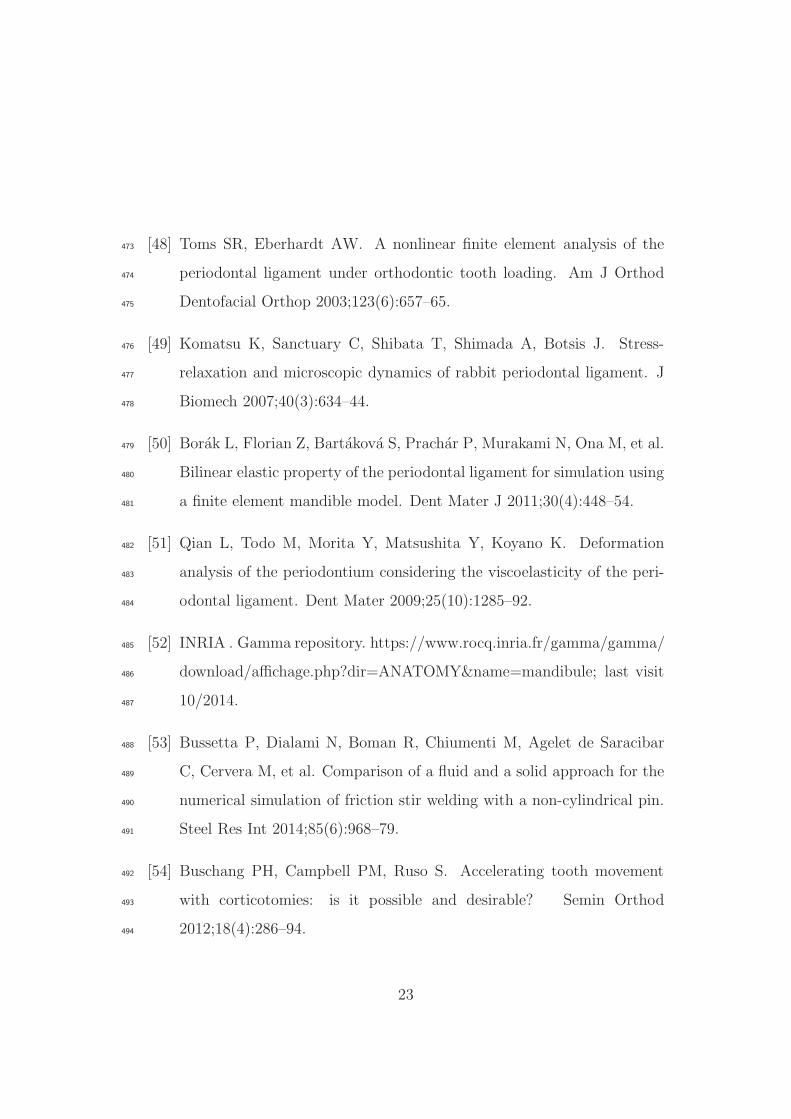
The first simulation was an academic case, testing the capacity of a re-129
modelling model combined with mesh management methods for tooth move-130
ment applications. A 2D single-rooted tooth was modelled with a root thick-131
ness of 7 mm at the alveolar margin and a root height of 16 mm, surrounded132
by alveolar bone (composed solely of trabecular tissue) 49-mm thick on each133
side of the tooth, and 40-mm high (see Figure 1). This model corresponded134
to a simulation of a tooth moving along the alveolar arch, with no other teeth135
present. The size of the considered bone reduced boundary effects to which136
remodelling algorithms are very sensitive [38, 39]. The tooth was considered137
as being a rigid tissue and the PDL was represented with a piecewise-linear138
interface model [16]. The bone was assumed to follow mechanical and remod-139
elling constitutive models such as described in [16, 30] with an initial uniform140
bone density of 1.3 gr/cc. These material and remodelling models assumed141
an anisotropic elastoplastic bone, submitted to remodelling in such a way142
that bone formation was observed at high strain energy density locations143
and bone resorption at low strain energy density locations. The coupling144
between the constitutive model and the remodelling model was expressed145
in a Continuum Damage Mechanics framework, with a remodelling criterion146
function of the strain energy density. Bone remodelling followed the concept147
of the mechanostat theory [40]: the bone density and orientation evolved148
according to the signed difference between the remodelling criterion and an149
7
homeostatic level of that value. All material and remodelling parameters150
are listed in Table 1. The remodelling rates are the only drivers of time in151
the remodelling algorithm and the all simulation. All time measures are thus152
described with respect to arbitrary time units, T. The bone was meshed with153
linear quadrangular elements using a structured mesh away from the tooth154
root in the regions delimited by the lateral rectangles ABHG and EFLK155
and using an unstructured mesh matching the root shape in its surround-156
ing in the region delimited by the central rectangle BEKH (see Figure 1)157
with a total of 1004 elements. This subdivision of the geometrical domain158
facilitated the mesh refinement in the area submitted to large strains around159
the apex of the tooth root. Boundary conditions were applied to represent160
the outcome of an orthodontic treatment at constant velocity. Boundary161
conditions representative of a end-of-treatment state, i.e. constant rate of162
displacement, were applied to the tooth. The tooth root was horizontally163
translated at a constant velocity to achieve a displacement of 1.5 times its164
width over 365 units of time. Rigid boundary conditions were applied to the165
bone basal line while it was restrained vertically on its top line and horizon-166
tally on its vertical extremities (see Figure 1). The ALE mesh movement was167
specified following the tooth kinematics to keep a good mesh quality along168
the displacement. The unstructured central mesh was moved with the same169
velocity as the tooth, imposing that the displacement of nodes B, H , and I170
was identical to that of node C in contact with the tooth root. In the same171
way, the displacement of nodes E, J , and K was identical to that of node D.172
The mesh nodes along the root surface (green curve in Figure 1) were relo-173
cated using spline curves [31]. Finally, the nodes of lines BC, DE, EK, KJ ,174
8
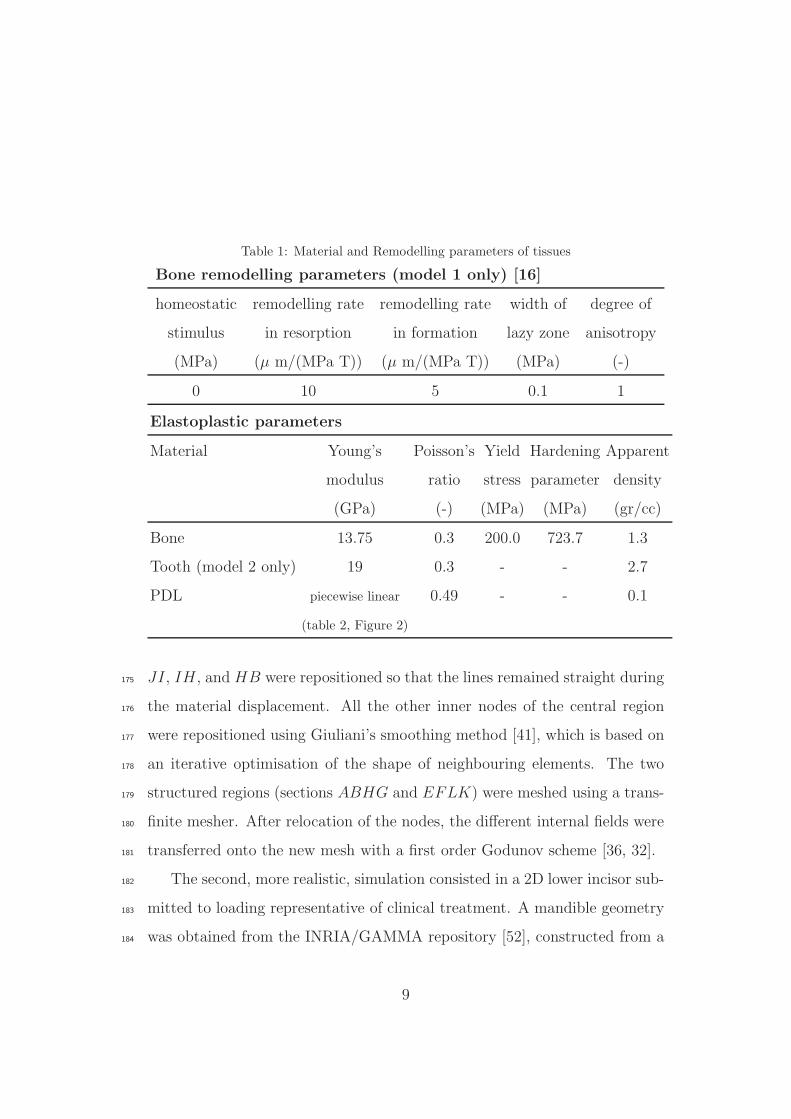
Table 1: Material and Remodelling parameters of tissues
Bone remodelling parameters (model 1 only) [16]
homeostatic remodelling rate remodelling rate width of degree of
stimulus in resorption in formation lazy zone anisotropy
(MPa) (µ m/(MPa T)) (µ m/(MPa T)) (MPa) (-)
0 10 5 0.1 1
Elastoplastic parameters
Material Young’s Poisson’s Yield Hardening Apparent
modulus ratio stress parameter density
(GPa) (-) (MPa) (MPa) (gr/cc)
Bone 13.75 0.3 200.0 723.7 1.3
Tooth (model 2 only) 19 0.3 - - 2.7
PDL piecewise linear 0.49 - - 0.1
(table 2, Figure 2)
JI, IH , and HB were repositioned so that the lines remained straight during175
the material displacement. All the other inner nodes of the central region176
were repositioned using Giuliani’s smoothing method [41], which is based on177
an iterative optimisation of the shape of neighbouring elements. The two178
structured regions (sections ABHG and EFLK) were meshed using a trans-179
finite mesher. After relocation of the nodes, the different internal fields were180
transferred onto the new mesh with a first order Godunov scheme [36, 32].181
The second, more realistic, simulation consisted in a 2D lower incisor sub-182
mitted to loading representative of clinical treatment. A mandible geometry183
was obtained from the INRIA/GAMMA repository [52], constructed from a184
9
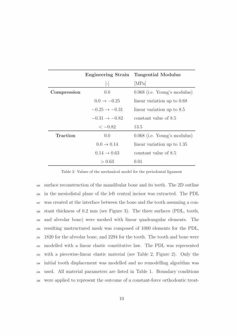
Engineering Strain Tangential Modulus
[-] [MPa]
Compression 0.0 0.068 (i.e. Young’s modulus)
0.0 → −0.25 linear variation up to 0.68
−0.25 → −0.31 linear variation up to 8.5
−0.31 → −0.82 constant value of 8.5
< −0.82 13.5
Traction 0.0 0.068 (i.e. Young’s modulus)
0.0 → 0.14 linear variation up to 1.35
0.14 → 0.63 constant value of 8.5
> 0.63 0.01
Table 2: Values of the mechanical model for the periodontal ligament
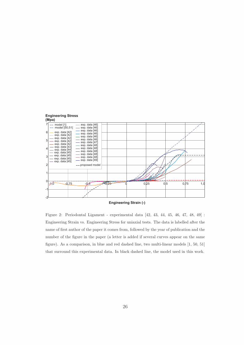
surface reconstruction of the mandibular bone and its teeth. The 2D outline185
in the mesiodistal plane of the left central incisor was extracted. The PDL186
was created at the interface between the bone and the tooth assuming a con-187
stant thickness of 0.2 mm (see Figure 3). The three surfaces (PDL, tooth,188
and alveolar bone) were meshed with linear quadrangular elements. The189
resulting unstructured mesh was composed of 1000 elements for the PDL,190
1820 for the alveolar bone, and 2294 for the tooth. The tooth and bone were191
modelled with a linear elastic constitutive law. The PDL was represented192
with a piecewise-linear elastic material (see Table 2, Figure 2). Only the193
initial tooth displacement was modelled and no remodelling algorithm was194
used. All material parameters are listed in Table 1. Boundary conditions195
were applied to represent the outcome of a constant-force orthodontic treat-196
10
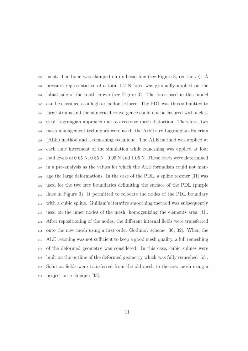
ment. The bone was clamped on its basal line (see Figure 3, red curve). A197
pressure representative of a total 1.2 N force was gradually applied on the198
labial side of the tooth crown (see Figure 3). The force used in this model199
can be classified as a high orthodontic force. The PDL was thus submitted to200
large strains and the numerical convergence could not be ensured with a clas-201
sical Lagrangian approach due to excessive mesh distortion. Therefore, two202
mesh management techniques were used: the Arbitrary Lagrangian-Eulerian203
(ALE) method and a remeshing technique. The ALE method was applied at204
each time increment of the simulation while remeshing was applied at four205
load levels of 0.65 N, 0.85 N , 0.95 N and 1.05 N. Those loads were determined206
in a pre-analysis as the values for which the ALE formalism could not man-207
age the large deformations. In the case of the PDL, a spline rezoner [31] was208
used for the two free boundaries delimiting the surface of the PDL (purple209
lines in Figure 3). It permitted to relocate the nodes of the PDL boundary210
with a cubic spline. Guiliani’s iterative smoothing method was subsequently211
used on the inner nodes of the mesh, homogenizing the elements area [41].212
After repositioning of the nodes, the different internal fields were transferred213
onto the new mesh using a first order Godunov scheme [36, 32]. When the214
ALE rezoning was not sufficient to keep a good mesh quality, a full remeshing215
of the deformed geometry was considered. In this case, cubic splines were216
built on the outline of the deformed geometry which was fully remeshed [53].217
Solution fields were transferred from the old mesh to the new mesh using a218
projection technique [33].219
11
3. Results220
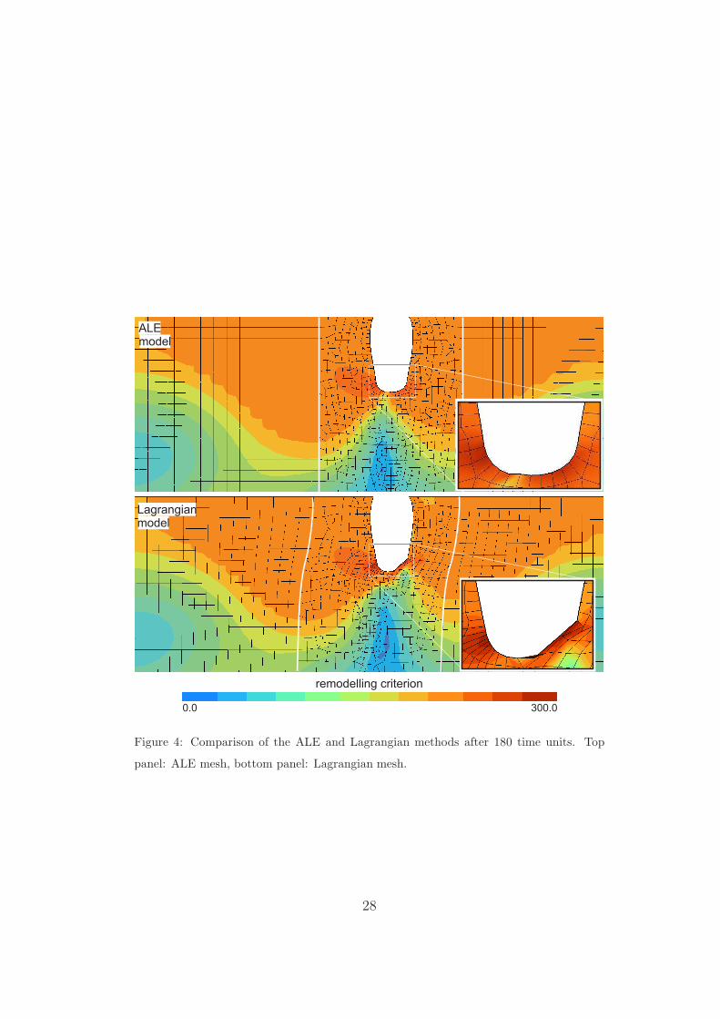
The benefit of the ALE method in the first model was analysed comparing221
the remodelling criteria values at 50% of the maximal displacement, i.e. 5.25222
mm (see Figure 4) with and without ALE. At that level of displacement,223
both methods showed the same results in the regions where the mesh is of224
good quality. However, the classical Lagrangian method produced a distorted225
mesh around the tooth apex to a point where the local numerical solution226
could not be trusted any more, with a remodelling criterion reaching high227
values around the tooth apex. Displacement higher than 5.4 mm could not be228
computed with a Lagrangian mesh due to negative jacobians while the ALE229
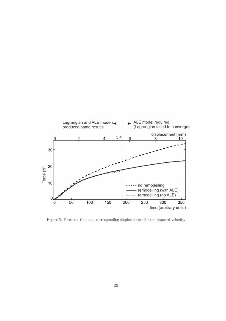
mesh allowed the full tooth displacement to be computed. The force needed230
for the ALE model (Figure 5 plain line) is the same as the one needed for231
the Lagrangian model (Figure 5 dash-dot line) where the Lagrangian mesh232
is of good quality (for the first 2.6 mm of translation). The Lagrangian force233
however deviates from the ALE one when the mesh becomes too distorted.234
The remodelling constitutive model facilitated the tooth movement, requiring235
a force about 40% lower than the force needed to displace the tooth of the236
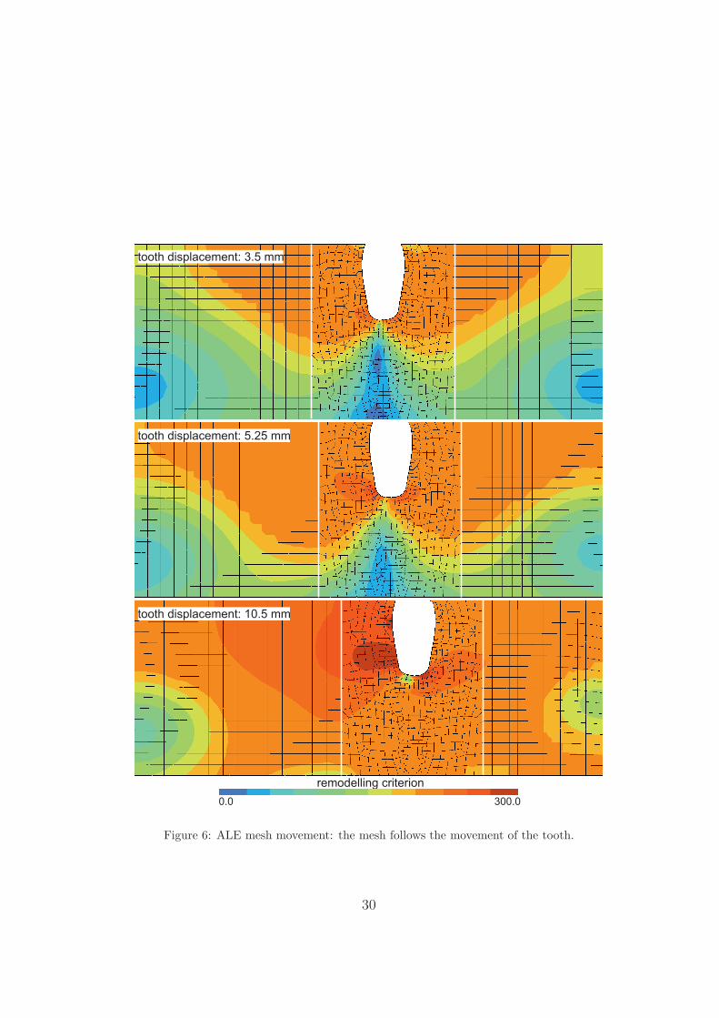
same length if no biological remodelling were present (Figure 5). The ALE237
mesh kinematics is depicted in Figure 6 were the remodelling criterion is238
plotted at three different time points of the simulation. The unstructured239
mesh around the tooth in the rectangle BEKH of Figure 1 followed the240
tooth movement. The structured mesh of the upstream rectangle ABHG241
expanded as the tooth moved away from the fixed left boundary while the242
structured mesh of the downstream rectangle EFLK shrunk.243
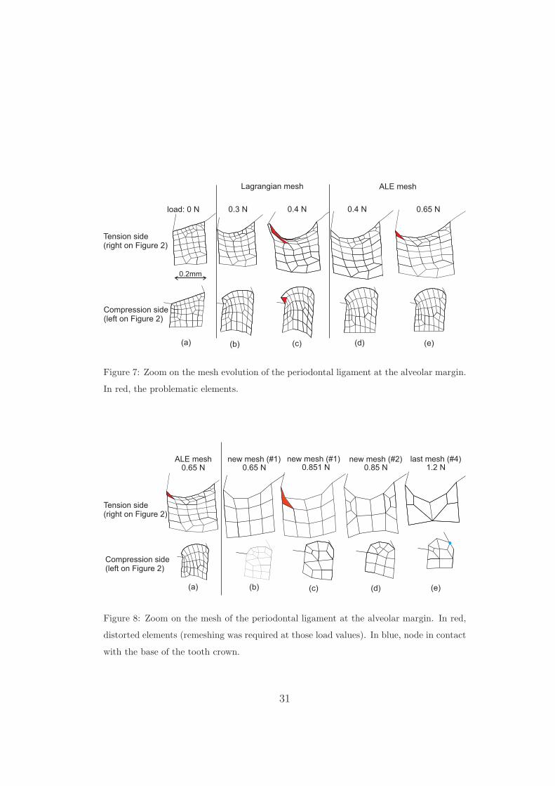
The forces applied on the second model led to large strains around the244
12
tooth collar. The soft PDL thus deformed up to a point where the mesh245
quality can not be trusted any more (see Figure 7(b)). A better represen-246
tation of the large strains at the alveolar margin without excessive mesh247
distortion was allowed by the ALE method (see initial and deformed meshes,248
with and without ALE in Figure 7(a-d)). A tipping force of 0.65 N was249
applied while keeping a good mesh quality but a higher force could not be250
used, with elements too distorted for a higher force, whatever the ALE node251
relocation algorithm used (Figure 7(e), red element). Indeed in the cervical252
area, because of the almost incompressible behaviour of the ligament, the free253
boundaries created convex and concave menisci so that inversion of the finite254
elements occured. The first load step defined for remeshing was when the255
applied load reached 0.65 N. The resulting new mesh (Figure 8(b)) allowed256
the computation to continue further (still applying the ALE method at each257
time step) up to a 0.85 N force. At a higher force level the mesh became once258
more too distorted on the tension side (Figure 8(c)). New remeshing instants259
were defined similarly at 0.85 N, 0.95 N, and 1.05 N. This fourth and final260
mesh was used for forces up to 1.2 N. This remeshing technique could be used261
further, every time defining new time steps at which remeshing takes place.262
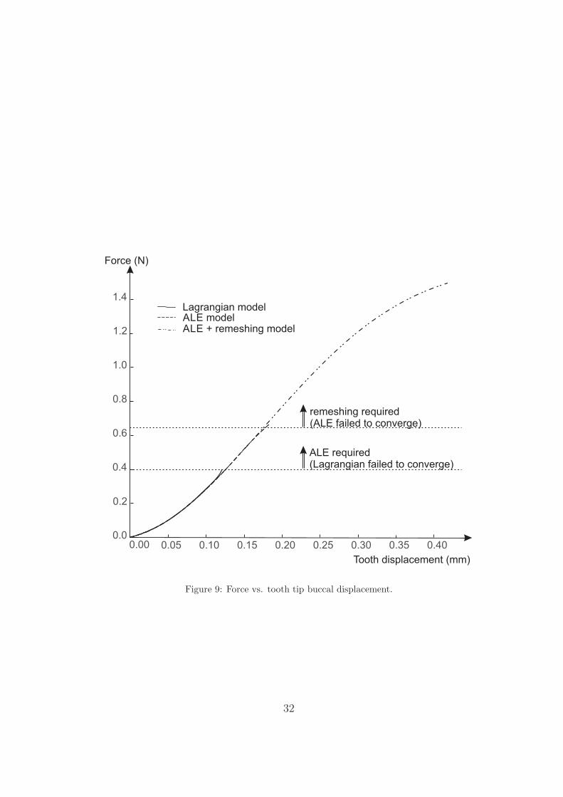
The displacement of the tooth tip was identical for all three models (purely263
Lagrangian, ALE, ALE with remeshing) as long as the model converged (see264
Figure 9).265
4. Discussion266
This work proposes an assessment of computational tools such as the Ar-267
bitrary Lagrangian Eulerian formalism and remeshing in the development of268
13
orthodontics tooth movement predictive models. Although this work focuses269
on the computational methods and the presented models are not validated270
against experimental and clinical data, it demonstrates the advantages and271
drawbacks of these methods for soft tissues modelling and remodelling mod-272
els.273
The first model shows that the ALE formalism makes it possible to reach274
a large displacement of a tooth within a mandible including the effect of275
bone remodelling without any remeshing steps. While the model is not rep-276
resentative of an actual tooth movement, it emphasizes the need to keep a277
good-quality mesh where remodelling is observed so that the bone formation278
or resorption is not artifically modified by numerical errors due to exces-279
sive mesh distortion. It should be emphasized that the aim of the proposed280
model is not clinically-driven. While the loading conditions have been cho-281
sen to represent average constant rate of displacement achieved in the third282
phase of orthodontic treatments [54, 55], the reproduced movement is not283
a model of an actual treatment. In particular, no physiological homeostatic284
loads are present, and the constant velocity condition is assumed to be the285
result of using orthodontic devices which are not modelled. It is unlikely286
that a constant rate of displacement would be achieved over such a distance287
without the need to adapt the device used.288
The second model underlines the possibility of reaching very large defor-289
mations in soft tissues models. The combination of the ALE formalism used290
continuously throughout the simulation with a remeshing algorithm used291
when needed facilitates the development of a reliable model of the menisci292
creation at the free boundaries of thin soft tissues. Analysing the evolution293
14
of the mesh in the periodontal ligament however shows that the number of294
elements describing those boundaries has to decrease with increasing applied295
load. The creation of the menisci due to the deformation needs an initial fine296
mesh. Once the menisci are formed, building a fine mesh without creating297
badly shaped elements at the extremities is very hard. At the tension side,298
the angle between the concave meniscus and the tooth boundary increases299
as the force increases, and become obtuse. At the compression side however,300
the angle between the convex meniscus and the bone boundary decreases,301
with a tendency to deform the quadrangles into triangles. Therefore, the302
description of the geometry of the free boundary is less and less accurate in303
order to be able to mesh it properly. Using the combination of ALE and304
remeshing methods in this case allows the simulation to reach force levels305
that are representative of orthodontic treatment force levels. This is a major306
improvement with respect to a purely Lagrangian approach that can only307
reach a force a quarter of the final value achieved here.308
3D models of a set of adjacent teeth submitted to loading through or-309
thodontic devices would however better represent an actual clincal outcome.310
Such models have already shown to perform well in initial tooth movement311
predictions and in long-term prediction when the remodelling algorithm in-312
volves full remeshing of a new geometry at each time step. In the case of313
remodelling algorithm such as used in this work, the presented applications314
demonstrate that the ALE formalism is a very efficient way to delay remesh-315
ing operations. The later are usually very expensive in terms of CPU time316
and user work time, even for 2D problems. In a 3D context, remeshing be-317
comes a major issue and we think that it could be partially solved by the318
15
ALE methods, which are already fully functional in 3D. Applications in 3D319
will be thus addressed in a near future.320
This computational work presents a promising approach to model large321
tooth displacements in orthodontic treatment. This approach is not limited322
to orthodontic treatment and can be used in combination with any remod-323
elling algorithm fully embedded within the constitutive law and not needing324
full computation of a new geometry.325
5. Author’s declarations326
Funding: None declared327
Conflicts of Interest: None declared328
Ethical Approval: Not required329
References330
[1] Cattaneo PM, Dalstra M, Melsen B. The finite element method : a tool331
to study orthodontic tooth movement. J Dent Res 2005;84(5):428–33.332
[2] Mackerle J. Finite element modelling and simulations in dentistry:333
a bibliography 1990-2003. Comput Methods Biomech Biomed Engin334
2004;7(5):277–303.335
[3] Van Staden RC, Guan H, Loo YC. Application of the finite element336
method in dental implant research. Comput Methods Biomech Biomed337
Engin 2006;9(4):257–70.338
16
[4] Provatidis CG. A bone-remodelling scheme based on principal strains339
applied to a tooth during translation. Comput Methods Biomech340
Biomed Engin 2003;6(5-6):347–52.341
[5] Chen J, Li W, Swain MV, Ali Darendeliler M, Li Q. A periodontal342
ligament driven remodeling algorithm for orthodontic tooth movement.343
J Biomech 2014;47(7):1689–95.344
[6] Li J, Li H, Shi L, Fok AS, Ucer C, Devlin H, et al. A mathematical model345
for simulating the bone remodeling process under mechanical stimulus.346
Dent Mater 2007;23(9):1073–8.347
[7] Bourauel C, Vollmer D, Jager A. Application of bone remodeling theo-348
ries in the simulation of orthodontic tooth movements. J Orofac Orthop349
2000;61(4):266–79.350
[8] Marangalou JH, Ghalichi F, Mirzakouchaki B. Numerical simulation of351
orthodontic bone remodeling. Orthod Waves 2009;68(2):64–71.352
[9] Qian Y, Fan Y, Liu Z, Zhang M. Numerical simulation of tooth move-353
ment in a therapy period. Clin Biomech 2008;23(Supplement 1):S48–52.354
[10] Kojima Y, Kawamura J, Fukui H. Finite element analysis of the ef-355
fect of force directions on tooth movement in extraction space closure356
with miniscrew sliding mechanics. Am J Orthod Dentofacial Orthop357
2012;142(4):501–8.358
[11] Soncini M, Pietrabissa R. Quantitative approach for the prediction359
of tooth movement during orthodontic treatment. Comput Methods360
Biomech Biomed Engin 2002;5(5):361–8.361
17
[12] van Schepdael A, De Bondt K, Geris L, Sloten JV. A visco-elastic model362
for the prediction of orthodontic tooth movement. Comput Methods363
Biomech Biomed Engin 2014;17(6):581–90.364
[13] Cronau M, Ihlow D, Kubein-Meesenburg D, Fanghnel J, Dathe H, Ngerl365
H. Biomechanical features of the periodontium: an experimental pilot366
study in vivo. Am J Orthod Dentofacial Orthop 2006;129(5):599.e13–21.367
[14] Field C, Li Q, Li W, Thompson M, Swain M. A comparative mechanical368
and bone remodelling study of all-ceramic posterior inlay and onlay fixed369
partial dentures. J Dent 2012;40(1):48–56.370
[15] Lin D, Li Q, Li W, Duckmanton N, Swain M. Mandibular bone remod-371
eling induced by dental implant. J Biomech 2010;43(2):287–93.372
[16] Mengoni M, Ponthot JP. A generic anisotropic continuum damage373
model integration scheme adaptable to both ductile damage and bio-374
logical damage-like situations. Int J Plasticity 2015;66:46–70.375
[17] Colciago C, Deparis S, Quarteroni A. Comparisons between reduced376
order models and full 3D models for fluid-structure interaction problems377
in haemodynamics. J Comput Appl Math 2014;265:120–38.378
[18] Martino ED, Guadagni G, Fumero A, Ballerini G, Spirito R, Biglioli379
P, et al. Fluid-structure interaction within realistic three-dimensional380
models of the aneurysmatic aorta as a guidance to assess the risk of381
rupture of the aneurysm. Med Eng Phys 2001;23(9):647–55.382
18
[19] Javadzadegan A, Fakhim B, Behnia M, Behnia M. Fluid-structure in-383
teraction investigation of spiral flow in a model of abdominal aortic384
aneurysm. Eur J Mech B Fluids 2014;46:109–17.385
[20] Langer U, Yang H. Partitioned solution algorithms for fluid-structure386
interaction problems with hyperelastic models. J Comput Appl Math387
2015;276:47–61.388
[21] Lee C, Zhang Y, Takao H, Murayama Y, Qian Y. A fluid-structure inter-389
action study using patient-specific ruptured and unruptured aneurysm:390
The effect of aneurysm morphology, hypertension and elasticity. J391
Biomech 2013;46(14):2402–10.392
[22] Taelman L, Degroote J, Swillens A, Vierendeels J, Segers P. Fluid-393
structure interaction simulation of pulse propagation in arteries: Nu-394
merical pitfalls and hemodynamic impact of a local stiffening. Int J Eng395
Sci 2014;77:1–13.396
[23] Wolters B, Rutten M, Schurink G, Kose U, de Hart J, van de Vosse F.397
A patient-specific computational model of fluid-structure interaction in398
abdominal aortic aneurysms. Med Eng Phys 2005;27(10):871–83.399
[24] Chiastra C, Migliavacca F, Martınez MA, Malve M. On the necessity400
of modelling fluid-structure interaction for stented coronary arteries. J401
Mech Behav Biomed Mater 2014;34:217–30.402
[25] Guivier-Curien C, Deplano V, Bertrand E. Validation of a numerical403
3D fluid-structure interaction model for a prosthetic valve based on ex-404
perimental PIV measurements. Med Eng Phys 2009;31(8):986–93.405
19
[26] McCormick M, Nordsletten D, Kay D, Smith N. Simulating left ventricu-406
lar fluid-solid mechanics through the cardiac cycle under LVAD support.407
J Comput Phys 2013;244:80–96.408
[27] Yin Y, Choi J, Hoffman EA, Tawhai MH, Lin CL. A multiscale MDCT409
image-based breathing lung model with time-varying regional ventila-410
tion. J Comput Phys 2013;244:168–92.411
[28] Kuhlmann M, Fear E, Ramirez-Serrano A, Federico S. Mechanical model412
of the breast for the prediction of deformation during imaging. Med Eng413
Phys 2013;35(4):470–8.414
[29] Potula S, Solanki K, Oglesby D, Tschopp M, Bhatia M. Investigating415
occupant safety through simulating the interaction between side curtain416
airbag deployment and an out-of-position occupant. Accid Anal Prev417
2012;49:392–403.418
[30] Mengoni M, Ponthot JP. An enhanced version of a bone remodelling419
model based on the continuum damage mechanics theory. Comput Meth-420
ods Biomech Biomed Engin 2015;18(12):1367–76.421
[31] Boman R, Ponthot JP. Efficient ALE mesh management for 3D quasi-422
Eulerian problems. Int J Numer Methods Eng 2012;92(10):857–90.423
[32] Boman R, Ponthot JP. Enhanced ALE data transfer strategy for explicit424
and implicit thermomechanical simulations of high-speed processes. Int425
J Impact Eng 2013;53:62–73.426
[33] Bussetta P, Boman R, Ponthot JP. Efficient 3D data transfer operators427
20
based on numerical integration. Int J Numer Methods Eng 2015;102(3-428
4):892–929.429
[34] Donea J, Huerta A, Ponthot JP, Rodriguez-Ferran A. Encyclopedia of430
Computational Mechanics, Volume 1; chap. 14: Arbitrary Lagrangian-431
Eulerian Methods. Stein, E. and de Borst, R. and Hughes T. J. R.; 2004,432
p. 413–37.433
[35] Benson DJ. An efficient, accurate, simple ALE method for non-434
linear finite element programs. Comput Methods Appl Mech Eng435
1989;72(3):305–50.436
[36] Rodriguez-Ferran A, Casadei F, Huerta A. ALE stress update for tran-437
sient and quasistatic processes. Int J Numer Methods Eng 1998;42:241–438
62.439
[37] Sarrate J, Huerta A. Efficient unstructured quadrilateral mesh genera-440
tion. Int J Numer Methods Eng 2000;49:1327–50.441
[38] Bitsakos C, Kerner J, Fisher I, Amis AA. The effect of muscle loading442
on the simulation of bone remodelling in the proximal femur. J Biomech443
2005;38(1):133–9.444
[39] Fernandez J, Garcıa-Aznar J, Martınez R. Numerical analysis of a445
diffusive strain-adaptive bone remodelling theory. Int J Solids Struct446
2012;49(15):2085–93.447
[40] Frost H. Skeletal structural adaptations to mechanical usage (SATMU):448
2. Redefining Wolff’s law: the remodeling problem. Anat Rec449
1990;226(4):414–22.450
21
[41] Giuliani S. An algorithm for continuous rezoning of the hydrodynamic451
grid in Arbitrary Lagrangian-Eulerian computer codes. Nucl Eng Des452
1982;72(2):205–12.453
[42] Dorow C, Krstin N, Sander FG. Determination of the mechanical prop-454
erties of the periodontal ligament in a uniaxial tensional experiment. J455
Orofac Orthop 2003;64(2):100–7.456
[43] Natali AN, Carniel EL, Pavan PG, Bourauel C, Ziegler A, Keilig L.457
Experimental-numerical analysis of minipig’s multi-rooted teeth. J458
Biomech 2007;40(8):1701–8.459
[44] Natali AN, Pavan PG, Carniel EL, Dorow C. A transversally isotropic460
elasto-damage constitutive model for the periodontal ligament. Comput461
Methods Biomech Biomed Engin 2003;6(5-6):pp. 329–336.462
[45] Aversa R, Apicella D, Perillo L, Sorrentino R, Zarone F, Ferrari M,463
et al. Non-linear elastic three-dimensional finite element analysis on464
the effect of endocrown material rigidity on alveolar bone remodeling465
process. Dent Mater 2009;25(5):678–90.466
[46] Pini M, Wiskott HWA, Scherrer SS, Botsis J, Belser UC. Mechani-467
cal characterization of bovine periodontal ligament. J Periodontal Res468
2002;37(4):237–44.469
[47] Pini M, Zysset PK, Botsis J, Contro R. Tensile and compressive be-470
haviour of the bovine periodontal ligament. J Biomech 2004;37(1):111–471
9.472
22
[48] Toms SR, Eberhardt AW. A nonlinear finite element analysis of the473
periodontal ligament under orthodontic tooth loading. Am J Orthod474
Dentofacial Orthop 2003;123(6):657–65.475
[49] Komatsu K, Sanctuary C, Shibata T, Shimada A, Botsis J. Stress-476
relaxation and microscopic dynamics of rabbit periodontal ligament. J477
Biomech 2007;40(3):634–44.478
[50] Borak L, Florian Z, Bartakova S, Prachar P, Murakami N, Ona M, et al.479
Bilinear elastic property of the periodontal ligament for simulation using480
a finite element mandible model. Dent Mater J 2011;30(4):448–54.481
[51] Qian L, Todo M, Morita Y, Matsushita Y, Koyano K. Deformation482
analysis of the periodontium considering the viscoelasticity of the peri-483
odontal ligament. Dent Mater 2009;25(10):1285–92.484
[52] INRIA . Gamma repository. https://www.rocq.inria.fr/gamma/gamma/485
download/affichage.php?dir=ANATOMY&name=mandibule; last visit486
10/2014.487
[53] Bussetta P, Dialami N, Boman R, Chiumenti M, Agelet de Saracibar488
C, Cervera M, et al. Comparison of a fluid and a solid approach for the489
numerical simulation of friction stir welding with a non-cylindrical pin.490
Steel Res Int 2014;85(6):968–79.491
[54] Buschang PH, Campbell PM, Ruso S. Accelerating tooth movement492
with corticotomies: is it possible and desirable? Semin Orthod493
2012;18(4):286–94.494
23

[55] Dixon V, Read M, O’Brien K, Worthington H, Mandall N. A randomized495
clinical trial to compare three methods of orthodontic space closure. J496
Orthod 2002;29(1):31–6.497
24
A B E F
G H I J K L
12mm 7mm 12mm
37mm 37mm
40mm
16mm
DC
Figure 1: Academic case: geometry, mesh, and ALE mesh management: the nodes on the
green curve are relocated using spline curves, the blue points have an horizontal displace-
ment which is set equal to the one of the red points, the blue lines are remeshed (with a
constant number of elements) as if they remained straight between their extremities.
25
-2
-1
0
1
2
3
4
5
6
7
-1,0 -0,75 0 0,25 0,5 0,75
Engineering Strain -( )
exp. data [42]exp. data [42]exp. data [42]exp. data [42]exp. data [42]
exp. data [44]exp. data [43]
exp. data [46]exp. data [46]exp. data [46]exp. data [46]exp. data [46]exp. data [46]exp. data [47]exp. data [48]exp. data [48]exp. data [48]exp. data [48]exp. data [48]
[1]model
proposed model
exp. data [49]
exp. data [45]exp. data [45]exp. data [45]exp. data [45]
Engineering Stress( )Mpa
1,0-0,5 -0,25
[50,51]model
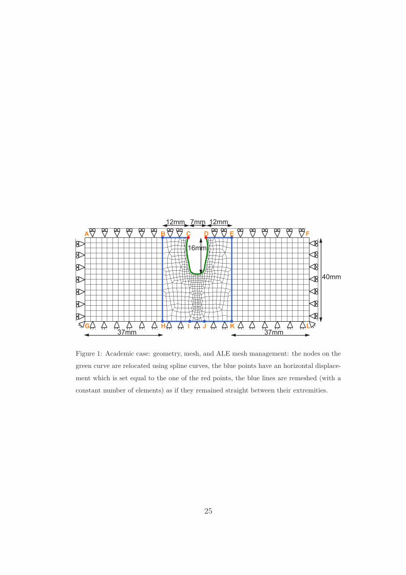
Figure 2: Periodontal Ligament - experimental data [42, 43, 44, 45, 46, 47, 48, 49] :
Engineering Strain vs. Engineering Stress for uniaxial tests. The data is labelled after the
name of first author of the paper it comes from, followed by the year of publication and the
number of the figure in the paper (a letter is added if several curves appear on the same
figure). As a comparison, in blue and red dashed line, two multi-linear models [1, 50, 51]
that surround this experimental data. In black dashed line, the model used in this work.
26
bone
tooth
PDL
clampedbasal bone
0.2mm
0.2mm
appliedpressure
PDL
PDL
Figure 3: 2D geometry in the mesiodistal plane of the left central incisor.
27
ALEmodel
Lagrangianmodel
remodelling criterion
0.0 300.0
Figure 4: Comparison of the ALE and Lagrangian methods after 180 time units. Top
panel: ALE mesh, bottom panel: Lagrangian mesh.
28
0
10
20
30
Forc
eN(
)
no remodelling
remodelling (with ALE)
0 2 4 6 8 10displacement (mm)
0 50 100 150 200 250 300 350
time (arbitrary units)
remodelling (no ALE)
5.4
ALE model required(Lagrangian failed to converge)
Lagrangian and ALE modelsproduced same resutls
Figure 5: Force vs. time and corresponding displacements for the imposed velocity.
29
remodelling criterion
0.0 300.0
tooth displacement: 10.5 mm
tooth displacement: 5.25 mm
tooth displacement: 3.5 mm
Figure 6: ALE mesh movement: the mesh follows the movement of the tooth.
30
0.2mm
(a) (e)(d)(c)(b)
load: 0 N 0.3 N 0.4 N 0.4 N 0.65 N
Lagrangian mesh ALE mesh
Tension side(right on Figure 2)
Compression side(left on Figure 2)
Figure 7: Zoom on the mesh evolution of the periodontal ligament at the alveolar margin.
In red, the problematic elements.
(a)
0.65 N
(b)
ALE mesh0.65 N
new mesh (#1)0.8 N51
new mesh (#1) new mesh (#2)
(c) (d)
1.2 Nlast mesh (#4)
(e)
0.8 N5
Tension side(right on Figure 2)
Compression side(left on Figure 2)
Figure 8: Zoom on the mesh of the periodontal ligament at the alveolar margin. In red,
distorted elements (remeshing was required at those load values). In blue, node in contact
with the base of the tooth crown.
31
0.0
0.2
0.4
0.6
0.8
1.0
1.2
1.4
0.00 0.05 0.10 0.15 0.20 0.25 0.30 0.35 0.40
ALE modelALE + remeshing model
Tooth displacement (mm)
Force (N)
remeshing required(ALE failed to converge)
Lagrangian model
ALE required(Lagrangian failed to converge)
Figure 9: Force vs. tooth tip buccal displacement.
32