MEMORANDUM To: From: Date: Subject: 1. Introduction
84
MEMORANDUM To: Dr. Michael Suplee, Montana Department of Environmental Quality From: Arun Varghese and Joshua Cleland Date: June 29, 2005 Subject: Seasonally Stratified Water Quality Analysis for Montana Rivers and Streams – Final Report 1. Introduction This memorandum presents ICF’s analysis of regionally based stratification methodologies for water quality criteria determination in Montana rivers and streams. The purpose of this analysis is to support the Montana Department of Environmental Quality (MT DEQ) as it develops nutrient and nuisance-algae criteria for flowing waters. This analysis builds upon research and analysis ICF performed for related project phases sponsored by the U.S. Environmental Protection Agency (EPA) and MT DEQ: • In a July 2004 report (ICF 2004b), we analyzed the relationships between ambient surface water quality and selected environmental and geospatial characteristics of Montana rivers and streams; and • In a November 2004 (ICF 2004a) report, we analyzed the relationship between the statistical distributions of water quality parameter observations at designated reference locations and in the whole population of observations from water quality monitoring locations in various classes of Montana rivers and streams. In the current analysis, most elements of the previous two phases of have been reworked with an expanded database and employing seasonal stratification as a further means of partitioning the data. In addition, the current analysis examines whether general purpose, regionally based stratifying methodologies such as Omernik ecoregions provide an adequate basis to establish geographic zones for nutrient criteria determination in the state of Montana. The analysis also examines using stream order and lithology data in combination with Omernik ecoregions to establish nutrient zones.
Transcript of MEMORANDUM To: From: Date: Subject: 1. Introduction

MEMORANDUM To: Dr. Michael Suplee, Montana Department of Environmental Quality
From: Arun Varghese and Joshua Cleland
Date: June 29, 2005
Subject: Seasonally Stratified Water Quality Analysis for Montana Rivers and Streams – Final Report
1. Introduction
This memorandum presents ICF’s analysis of regionally based stratification methodologies for water quality criteria determination in Montana rivers and streams.
The purpose of this analysis is to support the Montana Department of Environmental Quality (MT DEQ) as it develops nutrient and nuisance-algae criteria for flowing waters. This analysis builds upon research and analysis ICF performed for related project phases sponsored by the U.S. Environmental Protection Agency (EPA) and MT DEQ:
• In a July 2004 report (ICF 2004b), we analyzed the relationships between ambient
surface water quality and selected environmental and geospatial characteristics of Montana rivers and streams; and
• In a November 2004 (ICF 2004a) report, we analyzed the relationship between the
statistical distributions of water quality parameter observations at designated reference locations and in the whole population of observations from water quality monitoring locations in various classes of Montana rivers and streams.
In the current analysis, most elements of the previous two phases of have been reworked
with an expanded database and employing seasonal stratification as a further means of partitioning the data. In addition, the current analysis examines whether general purpose, regionally based stratifying methodologies such as Omernik ecoregions provide an adequate basis to establish geographic zones for nutrient criteria determination in the state of Montana. The analysis also examines using stream order and lithology data in combination with Omernik ecoregions to establish nutrient zones.

Section 2 of this memorandum describes the scope and objectives of this analysis. Section 3 identifies the sources of data ICF used for the analysis and explains how we compiled the data into a relational database. Section 4 describes the statistical methods used in the analysis. In Section 5, we present the results and conclusions of the analysis. Section 6 identifies the literature cited in this memorandum. Appendix A documents the methodologies used to group water quality parameters, Appendix B documents the methodologies used to group data by seasons, Appendix C describes the lithologic grouping methodology, and Appendix D provides the detailed results log files of the statistical analysis. 2. Scope and Objectives
EPA’s guidance on nutrient and algal criteria development (EPA 2000) recognizes the need for identifying stream groups with comparable biological, ecological, physical, and chemical features, because natural levels of nutrient concentrations in streams are likely to be related to these factors. Spatially defined nutrient zones developed by grouping streams with similar characteristics are therefore an appropriate mechanism of setting nutrient criteria that reflect natural variability.
A stratifying system that tends to minimize variability within nutrient zones and maximize differences between nutrient zones is considered suitable for setting nutrient criteria. Two approaches have previously been proposed in regulatory guidance and literature for delineating such nutrient zones: (1) general purpose regionalizations that depend on subjective expert judgment in identifying regions that are relatively homogenous in terms of a composite set of environmental variables such as geology, ecology, climate and land-use and (2) nutrient-specific regionalizations that depend on empirical analysis and data-mining approaches to identify regions that are relatively homogenous in terms of the concentration of a particular nutrient. While nutrient-specific regionalizations may potentially provide a higher level of homogeneity and statistical precision, general-purpose zones offer advantages in terms of their easy applicability and convenience.
To support the development of general-purpose nutrient zones for Montana, we used
statistical metrics to gauge the performance of potential general-purpose environmental stratifying methodologies. Specifically, we evaluated the Omernik ecoregions approach and improvised classifications based on Omernik ecoregions in combination with geological and hydrologic variables. The analyses were applied exclusively to Montana river and stream reaches, and the data were seasonally stratified to improve statistical precision. The analytical methods included tests to verify that the stratifications and sub-stratifications based on these parameters are statistically meaningful. We also computed alternative measures of variation to assess the effectiveness of the stratification methodologies. All analyses were conducted separately for the reference and whole population. Furthermore, the analyses were performed using all observed data, as well as station median data. The analyses based on station median data were expected to be more statistically robust.
Another objective of this project was to perform distributional analyses that would enable MT DEQ to use data from reference sites to develop nutrient and algal criteria within nutrient zones. EPA guidance (EPA 2000) recommends that the 75th percentile of the frequency distribution of water quality measurements at reference stream reaches be used to develop
2

nutrient criteria. In the absence of data for reference stream reaches, EPA guidance recommends choosing from the 5th to 25th percentile of the frequency distribution of the whole population of a class of streams to develop the criteria.1 Therefore, application of the EPA guidance requires not only the computation of the 75th percentile in reference population, but also comparison of this value with 5th to 25th percentile in the whole population. This analysis computes the 75th percentile of nutrient concentrations in the reference population and matches these to the whole population distribution to assess how the two populations are related for various potential nutrient zone groupings. This is effectively a revision of the analysis conducted in November 2004 (ICF, 2004b) using the updated database developed as part of this phase of the project.
A further objective of this analysis was to compare the distribution of stream order in the whole population data and the reference population data. This analysis was conducted for specific nutrients in Omernik level III ecoregions at both the observation level and the station level. This part of the analysis could potentially lay the groundwork for refined analyses based on bootstrapping or simulation methods that ensure appropriate representation of different stream orders in the determination of nutrient criteria. The analysis also tested for statistically significant differences in nutrient concentrations between seasons in Omernik level III ecoregions. 3. Data Sources and Database Development
The first step of this analysis was to compile sources of water quality data and selected environmental and geospatial characteristics into a single relational database. Most of the water quality data were available in a database ICF compiled for the previous phases of the analysis (ICF 2004a).2 ICF deleted reference data from the previously compiled database and then added water quality data from sampling sites in designated reference reaches as well as from a few non-reference reaches. These newly-added data were provided by MT DEQ3 and reflected more-refined screening techniques for identifying reference reaches, as well as new data sources. Specific details on the reference site screening methodology are provided by MT DEQ (2005).
Figure 3.1 displays the location and identity of the reference stations in the newly-added
MT DEQ data. Figure 3.2 displays the location of the general population and reference population
stations in the new database.
1 Hereafter, we refer to data for the reference stream reaches as the “reference population.” We refer to data for non-reference stream reaches as the “general population.” 2 See ICF (2004a and 2004b) for details about the sources of data used to create the database. 3 Email communication with Dr Michael Suplee, MT DEQ, April 18, 2005.
3

SFkWillo_245_C
SFkFlath_244_C
ChepatCk_194_C
EfkBullR_205_C
Deerhorn_202_C
RoaringL_241_C
SeymoreC_249_C
ODellCk9_236_C
ElkCk999_209_C
BigCk999_180_C
PineCk99_238_C wfkstl99_274_C
crookd99_200_Clfkrok99_222_W
calfck99_192_C
sfksun99_250_C
waldrn99_270_C
WyomingC_107_C
WoodyIsl_174_W
WolfCree_130_W
WillowCr_172_W
WillowCr_171_W
WillowCr_104_C
WillowCr_103_C
Whitewat_170_W
Whitewat_169_W
Whitetai_102_W
WFkPopla_126_W
WFkBeave_095_C
WESTFORK_129_WWESTFORK_128_W
WESTFORK_127_W
WESTFORK_099_W
TuleCree_164_W
TuleCree_092_W
TribofNF_091_C
Swiftcur_132_C
SUNRIVER_116_C
SpringCr_081_W
SouthFkS_080_C
SOUTHFKF_115_C
SilverCr_078_C
SeymourC_076_C
SchaferC_074_C
RockCree_071_C
RockCree_070_C
ROARINGL_069_C
RoaringL_068_C
PumpkinC_161_W
PryorCre_159_C
PintlerC_066_C
PastureC_065_WPastureC_064_W
OFallonC_062_W
OFallon9_157_W
OFallon9_156_W
NoManCre_059_C
NFKGreen_058_C
Mussigbr_154_C
MuddyCre_057_W
MooseCre_056_C
MillUp99_053_C
LonePine_051_C
LittlePo_050_W
GoatCree_043_C
Gallatin_040_C
FishCree_038_W
EFkBullR_025_C
EagleCre_030_W
EagleCre_028_C
E.Redwat_027_W
DeerCree_023_C
CROOKEDC_111_C
CowCreek_141_W
CowCreek_022_W
Cottonwo_021_C
ClearCre_121_W
ChickenC_019_C
ChepatCr_108_C
CedarCr9_140_W
CalfCree_017_C
CabinCre_016_C
BrownsCr_015_C
BoxElder_138_W
Blacklea_008_W
Blackfoo_006_CBeaverCr_002_W
Beauvois_136_W Beauvais_131_W
BasinCre_001_C
ArrowCre_135_W
LittleMi_152_W
LittleLa_049_C
LittleDr_151_W
Highwood_044_W
CascadeC_193_CFourMile_212_C
nfktet99_234_C
WESTFORK_118_C
WaldronC_117_C
SeeleyCr_075_C
SCottonw_073_C
ROCKCREE_133_W
ROCKCREE_125_W
RockCree_124_W
RockCree_123_W
RockCrBL_122_W
NFkTeton_114_C
Fourmile_112_C
ElkSprin_037_C
EastRose_033_C
EASTFORK_031_C
BoxElder_382_W
BoxElder_137_W
BoxElder_013_W
Blacklea_007_C
BitterCr_120_W
BIGCREEK_110_C
ARMSTRON_109_W
LaMarche_048_C
LAKEFORK_113_C
0 50 100 150 20025Miles
LegendReference Sampling Stations
Ecological RegionsNorthern Rockies
Idaho Batholith
Middle Rockies
Wyoming Basin
Canadian Rockies
Northwestern Glaciated Plains
Northwestern Great Plains
Map 1: Reference Sampling Stations

M O N T A N AM O N T A N A
0 50 100 150 20025Miles
Legend
Reference Sampling Stations
General Population Stations
Ecological RegionsNorthern Rockies
Idaho Batholith
Middle Rockies
Wyoming Basin
Canadian Rockies
Northwestern Glaciated Plains
Northwestern Great Plains
Map 2: General Population and Reference Sampling Stations
ICF used the following steps to integrate the new and previously compiled data:
The existing database was updated for Strahler stream order using new data provided by MT DEQ that related Strahler stream order to sampling stations.
The updated version of the existing database (with reference data deleted) was
appended to the new data provided by MT DEQ. A number of queries were designed to check for duplicate observations, which were identified and deleted. New fields were introduced to indicate whether the data related to a reference reach, and to indicate the origin of the data.
The water quality data, which included latitude and longitude coordinates for each
observation, were spatially joined to GIS layers containing information on the stratifying parameters of interest. In particular, using a spatial join, each observation was assigned appropriate values for each stratifying parameter depending on the location of the sampling site. The stratifying parameters thus incorporated into the database include Omernik level III ecoregions, Omernik level IV ecoregions, geologic formation, and elevation. Elevation does not play a role in this analysis but was included in the database for later use by MT DEQ.
ICF created two stratifying parameters specifically for this analysis:
o “Grouped level III ecoregions” creates superecoregions, which represent a coarser
stratification than level III ecoregions. This stratification divides the state into Mountain and Prairie areas. The Mountain areas comprise the following level III ecoregions: Northern Rockies, Idaho Batholith, Middle Rockies and Canadian Rockies. The Prairie areas comprise the Wyoming Basin, Northwestern Glaciated Plains and Northwestern Great Plains.
o “Grouped Strahler Stream Order” groups together stream orders 1&2, 3&4, 5&6, and 7&8, respectively, in order to increase sample size in each category without significant loss of hydrologic similarity.
The previously compiled water quality data, which were obtained from Legacy
STORET, were collected by various agencies using various methods. A methodology developed by MT DEQ was used to group related water quality parameters. The objective of the water quality parameter grouping methodology was to group fundamentally equivalent analytic measurements, while avoiding double counts. A detailed explanation of the parameter grouping methodology is provided in Appendix A.
The water quality data were seasonally defined as Winter, Runoff, or Growing using
a methodology developed by MT DEQ. A detailed explanation of the seasonal grouping methodology is provided in Appendix B.
6

MT DEQ had previously provided ICF with data on lithologic classifications (e.g., rock types) within Montana (ICF, 2004b). The data were supplied in a GIS shapefile on a CD-ROM and were originally developed by Raines and Johnson (1996). The lithological classification shapefile contained over 80 groupings (i.e., rock types). Following the GIS-based spatial join, ICF combined these into 19 major lithologic categories according to a methodology proposed by MT DEQ, which is described in Appendix C. Lithologic classifications are also referred to as geologic formations in this analysis.
To eliminate potentially erroneous or highly uncertain data from the assessment, ICF
excluded water quality data associated with certain comment codes4 in the Legacy STORET data. For example, these codes denoted estimated values or values from analyses known to be in error.
In addition, ICF replaced Legacy STORET data bearing comment codes5 denoting
non-detects with values equal to 50 percent of the reported detection limits.
ICF also eliminated from use all water quality parameters that had reported values of zero. Most analytical results in the database provided a result value and a detection limit, or an indication that the analyte was below the detection limit. True analytical values of zero are very unlikely (Luce, 2005), and therefore these data (most of which are old) were not used.
The resulting database is referred to hereafter as the “all-observation database.” We then processed the all-observation database to develop a “median database” as an
alternative basis for analysis. The median database contains a unique observation for each nutrient, for each station, for each season. This observation is the median observed value for a nutrient, at a particular station, in a particular season. The median database is less likely to be influenced by outliers and is more amenable to parametric statistical analysis. Analyses based on station median data are therefore expected to be more statistically robust. Many of the analyses conducted in this assignment were performed for both the total database and median database. However, many of the results summarized in this report are based on the median database.
The software used in the creation of the combined database included Arcview GIS, Stata (version 7), Microsoft Access and Microsoft Excel. 4. Statistical Methods
This section discusses the statistical methods employed in the following components of the analysis:
4 Specifically, ICF eliminated Legacy STORET data bearing comment-codes H, O, Q, L, Y and “*”; USGS data bearing comment code E; and estimated data bearing comment code J (with the exception of benthic chlorophyll-A data bearing comment code J.) 5 The specific legacy STORET comment codes included T, M, W, K, U, ND,”<” and “Non-detect.”
7
Mapping percentiles of interest from the reference population to the general population;
Testing of different stratification methodologies;
Computing measures of variance for alternative stratification methodologies;
Examining seasonal differences in nutrient concentrations; and
Analyzing stream order distributions in the general and reference populations.
For all analyses, ICF performed a series of statistical calculations by means of programs
written in Stata (version 7), a statistical analysis software package. ICF ran the Stata program for each water quality parameter for various combinations of stratifying parameters. Coarse-scale stratifications refer to stratifications based on a single stratifying parameter. Fine-scale stratifications refer to stratifications based on two stratifying parameters, one embedded or sub-stratified within the other. The results of the Stata runs are presented in Appendix D, along with a guide to their interpretation.
Most analyses were conducted separately for the general population and the reference population. Certain analyses were conducted exclusively on the all-observation database, other analyses exclusively on the median database, and some analyses were performed on both databases. Most analyses were performed for all seasons as well as for specific seasons.
Sections 4.1 through 4.5 provide further explanation of each component of the statistical analysis. Section 4.6 describes ICF’s quality assurance measures for the statistical results. 4.1 Percentile Mapping
Percentile mapping was performed using only the all-observation database. The percentile mapping methodology included four steps:
Computing summary statistics to describe the reference, non-reference, and whole
population characteristics for alternative stratification methodologies;
Performing tests of equality of populations to assess whether the reference and non-reference populations within each level of each stratification could be considered similar; and
Matching the reference and whole population distributions within each level of each
stratification methodology.
ICF performed the percentile matching only when four or more observations were available at non-reference and reference locations. Results were reported for each specific season and for all seasons combined. Each step in the percentile mapping analysis is described further below.
8
4.1.1 Summary Statistics for Reference and Whole Population
Summary statistics in the Stata results characterize the reference, non-reference, and whole population statistical distributions for the selected water quality parameter for each value of the stratifying or sub-stratifying parameter. Statistics are reported for the all-observation database and not the median database. Specific summary statistics include the total number of observations, minimum, maximum, mean, standard deviation and skewness for reference observations, non-reference observations, and whole population observations. In addition, the summary statistics include the values of the 10th, 25th, 50th, 75th, and 90th percentiles for reference observations, non-reference observations, and whole population observations. 4.1.2 Tests of Equality of Populations
ICF performed the Kolmogorov Smirnoff Test and the Kruskal Wallis Test to determine whether the reference and non-reference populations could be considered different from each other. Both tests were applied at the 95 percent confidence limit to determine if the null hypothesis of equality of the two populations could be rejected. (The Kolmogorov Smirnoff test assesses the equality of the entire distributions, while the Kruskal Wallis test assesses the equality of the medians of the populations.)
4.1.3 Percentile Matching
The statistical analysis program matched water quality parameter values in the reference and whole population distributions to find the percentiles in the whole population distribution that correspond to the percentiles of interest (i.e., 75th and 90th percentiles) in the reference population. Specific steps in this approach are listed below:
1. Compute the water quality parameter value corresponding to the percentile of interest in the reference population.
2. Generate a cumulative distribution function that calculates a percentile rank for each water quality parameter value in the whole population.
3. Determine the percentile in whole population that corresponds to the water quality
parameter value of the percentile of interest in the reference distribution.6 4. Generate box-whisker plots of nutrient concentrations at reference and non-reference
sites for each level of each stratification and for each season.
The text-format log files produced by the statistical program include the percentile matching results for each reference population percentile of interest.
6 ICF used a linear interpolation method in this step. ICF also tested a cubic interpolation method. However, in most cases the cubic interpolation method did not differ from the linear method. In a few cases, the cubic interpolation method resulted in missing values. Therefore, ICF decided to apply the linear interpolation method exclusively for this analysis.
9

4.2 Testing of Stratification Methodologies
This analysis was performed exclusively on the median database (described in Section 3) for various stratification and sub-stratification methodologies. Results were reported for all seasons and for specific seasons.
The results of the Stata runs included:
Summary statistics describing the statistical distribution of each water quality parameters for coarse and fine-scale stratifications;
Parametric and non-parametric statistical tests to assess whether stratifications and
sub-stratifications are statistically significant; and
Box-whisker plots for each coarse-scale stratifying parameter for each nutrient for each season.
4.2.1 Summary Statistics by Stratum
Summary statistics in the Stata results characterize the statistical distributions for the selected water quality parameter for each level of the stratifying or sub-stratifying parameter. All statistics are reported only for the median database. Specific summary statistics include the total number of observations, minimum, maximum, mean, standard deviation and skewness. In addition, the summary statistics include the values of the 10th, 25th, 50th, 75th, and 90th percentiles. 4.2.2 Non-Parametric Tests for Differences Between Stratified Populations
A stratification methodology may be considered statistically significant if there are differences in nutrient concentrations between the strata defined by the methodology, i.e., if at least one stratum may be considered to have a higher or lower median or mean concentration than the other strata. In order to test for statistically significant differences between the median nutrient concentrations of different strata within a given stratification methodology, ICF used the non-parametric Kruskal Wallis test. The test was used only on the median database. A 95 percent confidence level was used to identify statistically significant differences.
If the test indicated the existence of statistically significant differences in median concentrations between the strata, a post-hoc non-parametric multiple comparison test was implemented based on procedures described in Siegel and Castellan (1988). These procedures helped determine whether specific strata could be considered different from one another.
10

4.2.3 Parametric Tests for Differences Between Stratified Populations
In order to test for statistically significant differences between the mean nutrient concentrations of different strata within a given stratification methodology, ICF used analysis of variance (ANOVA) tests.
ANOVA procedures are most accurate when the underlying populations are normally
distributed with equal variance in each stratum. To determine if the data could be considered normally distributed for each nutrient for each stratification methodology, ICF performed the Shapiro-Wilk test of normality and assessed normal probability plots. In general, the hypothesis of normality could not be rejected for log-transformed data in the median database. (The all-observation database did not show the same characteristics; the log-transformed data in that database could not usually be considered normally distributed. Therefore, the all-observation database was not used for significance testing procedures.)
The Levene test was performed to determine if the data could be considered homoscedastic (having equal variance in each stratum) for each nutrient for each stratification methodology. In many cases, the hypothesis of homoscedasticity was rejected. However, the absolute value of the ratio of standard deviations across strata was most often less than two.
A consultation with ICF’s statistician (Cohen, 2005) concluded that ANOVA results were likely to be robust to these levels of non-normality and heteroscedasticity.
ANOVA was implemented only on the median database. A 95 percent confidence level was used to identify statistically significant differences.
If the test indicated statistically significant differences in mean concentrations between the strata, a post-hoc parametric multiple comparisons of means was performed using the Bonferroni adjustment.
In order to test the statistical validity of sub-stratification, we used a nested ANOVA model with sub-strata nested within the main strata. We then used the Wald test to test the significance of the sub-stratification term in the nested model. The Wald test is a way of testing the significance of particular explanatory variables in a statistical model. The Wald test works by comparing the performance of the unrestricted model with a restricted model in which the variables to be tested have been dropped. If the Wald test is significant for a particular explanatory variable or group of explanatory variables, then we would conclude that the parameters associated with these variables are not zero, and that the variables should be included in the model. If the Wald test is not significant then these explanatory variables can be omitted from the model. Further details on the Wald test may be found in Statacorp (2001).
The R2 and adjusted R2 statistics were computed for all ANOVA runs. Ideally, however,
these measures should not be used to select between alternative statistically valid stratification methodologies, because adding variables or sub-strata to a model will always improve the R2
measure. Instead, once a set of statistically significant stratification methods have been determined, the selection of the optimal method may be based on a priori ecological, biological,
11

and hydrogeologic considerations and practical ease of applicability. More complex model selection methods, such as those based on the Akaike Information Criterion statistics or the Davidson and MacKinnon J test, were not included in this analysis. 4.3 Computation of Measures of Variance for Alternative Stratification Methods
For the purposes of this project, a suitable stratification methodology is one that can be used to define nutrient zones in Montana between which nutrient concentrations differ from one another, and within which the variability of nutrient concentrations is minimized. Section 4.2 discussed tests to ascertain statistically significant differences between nutrient zones. To assess the performance of alternative stratification methodologies in minimizing variation within nutrient zones, two measures of variance were computed: the mean coefficient of variation and the coefficient of efficiency. 4.3.1 Mean Coefficient of Variation
For each stratification methodology, the mean coefficient of variation (MCV) was computed as follows, based on a definition provided in Robertson et al. (2001):
NnCV
MCV ∑ ×=
)( 2
XStDevCV =
where,
CV is the coefficient of variation of each group (or area); n is the number of observations in each group; N is the total number of observations in all of the groups; StDev is the standard deviation of each group; and
X is the mean concentration of each group.
One shortcoming of the MCV measure is that it is likely to improve (i.e., show lower absolute values) with increasing stratification. Therefore it would only be appropriate to use the MCV to assess the performance of alternative stratification schemes if the schemes divide the state into roughly equal number of strata. 4.3.2 Coefficient of Efficiency
Legates and McCabe (1999) proposed the coefficient of efficiency as a means of evaluating the goodness-of-fit of hydrologic and hydroclimatic models. This measure is defined as follows:
12

∑∑
−
−−=
i i
iii
OO
POCOE 2
2
)(
)(1
where,
iO = Value of the ith observation
iP = Predicted value corresponding to the ith observation (equal to the mean of the observations in the stratum of the ith observation) O = Grand mean of observed values
Thus, the COE in this analysis will equal the ANOVA R2.
This measure can vary from minus infinity (poor model) to 1.0 (perfect model).
Like the MCV, the COE has the shortcoming of being likely to improve with increasing stratification. Therefore it would only be appropriate to use the COE to assess the performance of alternative stratification schemes if the schemes divide the state into roughly equal number of strata.
Although the MCV and COE will usually be negatively correlated (i.e., high MCV associated with low COE and vice versa), there may be exceptions to this trend. These exceptions may occur because the MCV is weighted by the number of observations in each group and because the COE is more sensitive to departures from the grand mean. 4.4 Examination of Seasonal Differences in Nutrient Concentrations
In order to determine whether nutrient concentrations within nutrient zones differ by season, a limited analysis was performed for nutrient zones based on Omernik level III ecoregions. This analysis included:
Summary statistics; Non-parametric tests for between-season differences; and Parametric tests for between-season differences.
4.4.1 Summary Statistics by Season
Summary statistics in the Stata results characterize the statistical distributions for the selected water quality parameter by season for each Omernik level III ecoregion. All statistics are reported for both the all-observation database and the median database. Specific summary statistics include the total number of observations, minimum, maximum, mean, standard deviation and skewness. In addition, the summary statistics include the values of the 10th, 25th, 50th, 75th, and 90th percentiles.
13

4.4.2 Non-parametric tests for between season differences
In order to test for statistically significant differences between the median nutrient concentrations in different seasons of a given Omernik level III ecoregion, ICF used the non-parametric Kruskal Wallis test. The test was used for both the median database and the all-observation database. A 95 percent confidence level was used to identify statistically significant differences.
If the test indicated statistically significant differences in median concentrations between the seasons, a post-hoc non-parametric multiple comparison test was implemented based on procedures described in Siegel and Castellan (1988). These procedures help determine whether specific seasons may be considered different from one another.
4.4.3 Parametric tests for between season differences
In order to test for differences between the mean nutrient concentrations of different seasons within a given Omernik level III ecoregion, ICF implemented analysis of variance (ANOVA) tests on the log-transformed data. The tests were implemented for both the median database and the all-observation database.
Although ANOVA procedures are most accurate when the underlying populations are normally distributed with equal variance in each stratum, no specific tests were performed to verify that these conditions were met. On the basis of the exploratory data analysis undertaken earlier in the analysis, we assumed that departures from these conditions are not sufficient to bias the accuracy of the results. However, the results of the non-parametric tests are preferred in assessing seasonal trends.
If ANOVA indicated the existence of statistically significant differences in mean concentrations between the seasons, we performed a post-hoc parametric multiple comparisons of means using the Bonferroni adjustment. 4.5 Distribution of Stream Order in the Reference and General Populations
Higher stream orders often are associated with higher levels of nutrient concentrations as a result of increased natural and anthropogenic loadings. Regulators setting nutrient criteria would therefore be interested in knowing the distribution of stream order amongst reference sites in each nutrient zone for the available sample of water quality data. A preponderance of lower-order streams may suggest that a criterion based on the sample could be environmentally conservative. On the other hand, if higher order streams predominate, criteria based on the sample may not be sufficiently environmentally conservative. While the ideal distribution of stream order in the reference sample is an issue best judged by regulators, this analysis attempts to support this process by providing a distributional analysis of stream order in the reference and general populations. Future criteria-setting analyses that use bootstrapping or simulation methods to generate appropriately balanced and representative distributions of reference and general population data may also benefit from this groundwork.
14

Distributions of stream order were provided for the all-observation database as well as for
the median database (which represents individual stations). The analyses are provided by nutrient for each Omernik level III ecoregion for all seasons only. 4.5.1 Histograms of Strahler Stream Order Distribution
Histograms representing the proportion of observations/stations from each stream order were developed for the reference and general populations. A normal distribution curve was superimposed on the histograms. These graphs are developed for each nutrient for each level III ecoregion.
4.5.2 Tabulation of Strahler Stream Order
The Stata runs present a breakdown of the distribution of Strahler stream order in the reference and general population for each nutrient for each level III ecoregion. 4.5.3 Tests for Differences in Stream Order Distribution
The Pearson Chi-square test was performed to test for statistically significant differences in the distribution of stream order between the reference and general population.
The Kruskal Wallis test was also performed. However, this test is less appropriate than the Pearson Chi-square test, because the stream order variable is treated as an ordinal variable instead of as a categorical variable for this test. The results of the Pearson Chi-square test should therefore be preferred. 4.6 Quality Assurance
The quality assurance methodology ICF adopted for this analysis involved replication of randomly selected cases from the Stata log files in independent database management and statistical software. Specifically, the data pertinent to the randomly selected cases were independently queried and analyzed with Statistica, a competing statistical analysis software application. Because the Stata and Statistica results were in agreement for all QA cases, we concluded that the quality assurance analysis validated the querying system, the program, and the analysis conducted in Stata. For some cases, the QA was conducted in Stata but outside of the programming framework, in order to serve as a check on the integrity of the programs. 5. Results and Conclusions
ICF performed the suite of statistical analyses described in Section 4 for ten water quality parameters and several stratification and sub-stratification methodologies. As described in Section 4, some analyses were performed on the all-observation database, some analyses on the median database, and some analyses were performed on both databases. All analyses were seasonally stratified.
15

Because the suite of statistical analyses produced a very large amount of results, this section presents only the most interesting trends as well as summary tables for each type of analysis. The full results of the statistical analyses were saved in easily readable, self-explanatory, computer-generated text files, referred to as log files, which are included in Appendix D. A guide to locating and reading the log files also is included in Appendix D. In the tables presented in this section, water quality parameters are represented by a set of abbreviations. A key to these abbreviations is presented below.7 5.1 Percentile Mapping
Tables 5.1.1 through 5.1.4 present the 75th and 90th reference percentile equivalents in the whole population for each Omernik level III ecoregion for seven nutrients, benthic chlorophyll a and two turbidity parameters for each season and for all seasons combined. The summary statistics in these tables were computed without ammonia, benthic chlorophyll and turbidity. Ammonia was excluded from the summary statistics because it is very often at or below detection level in oxygenated surface waters, and oxygenated surface waters comprise the bulk of the data being analyzed. In general, bacteria rapidly convert ammonia N to its dominant and most oxidized form, NO3 (ICF, 2004a). We excluded turbidity and benthic chlorophyll data from the summary statistics in the tables because MT DEQ requested that turbidity and benthic chlorophyll be analyzed separately from nutrients. It is apparent from Tables 5.1.1 through 5.1.4 that seasonal trends are not very pronounced in the percentile mappings. The only exception to this finding is for the Middle Rockies and the Canadian Rockies in which the general population percentiles corresponding to the 75th and 90th percentile in the reference population are lower in the Winter season than for other seasons. Cross-nutrient trends suggest that the Northwestern Glaciated Plains and the Northwestern Great Plains are fairly homogeneous in their reference and general population distributions for all nutrients for all seasons. For the Northern Rockies, however, the 75th and 90th reference percentiles correspond to fairly low general population percentiles.
7 BNCHLOR-A = Benthic Chlorophyll-A; NO3+NO2 = Nitrates and Nitrites; SRP = Soluble Reactive Phosphates; TDP=Total Dissolved Phosphorus; TKN = Total Kjeldahl Nitrogen; TOTALN = Total Nitrogen; TOTALP = Total Phosphorus; TURB-JTU = Turbidity (JTUs); TURB-NTU = Turbidity (NTUs)
16

Table 5.1.1: Cross-Nutrient Percentile Matching Summary for Level III Ecoregions (All Seasons)
p75 p90 p75 p90 p75 p90 p75 p90 p75 p90AMMONIA - - 17.74 45.54 13.03 13.03 80.67 91.36 39.36 63.35
BNCHLOR-A - - 31.24 50.31 54.84 93.55 69.95 88.14 57.26 71.57NO3+NO2 47.43 59.41 26.24 73.57 82.18
SRP 16.76 23.12 54.17 83.38 85.21TKN 49.06 60.19 65.84 90.64 92.43
TOTAL N - 78.72 76.67 88.32 88.26TOTAL P 3.27 52.39 29.83 89.63 96.03
TDP - - - 96.38 97.85
Mean 29.13 54.77 50.55 86.99 90.33Std Dev 22.76 20.20 22.08 7.79 6.17
CV 0.78 0.37 0.44 0.09 0.07
31.52 37.73 18.52 48.8 75.7715.56 8.87 45.46 63.88 80.1226.38 43.71 52.06 80.59 68.33
- 74.69 61.67 66.13 72.113.27 27.4 25.65 81.02 85.13
- - - 84.44 95.59TURB-JTU - - - - - - - - 89.14 98.03TURB-NTU - - 76.14 91.74 55.59 63.55 92.21 96.31 70.1 75.16
19.18 38.48 40.67 70.81 79.5112.52 24.18 18.10 13.71 9.84
0.65 0.63 0.44 0.19 0.12
Water Quality
Parameter
Summary Statistics Exclude Ammonia, Benthic Chlorophyll and Turbidity
Great PlainsNorthwestern NorthwesternNorthern Middle Canadian
Rockies Rockies Rockies Glaciated Plains
Table 5.1.2: Cross-Nutrient Percentile Matching Summary for Level III Ecoregions (Winter)
p75 p90 p75 p90 p75 p90 p75 p90 p75 p90AMMONIA - - 16.76 43.27 - - 82.79 84.5 47.55 60.89
BNCHLOR-A - - - - - - - - - -NO3+NO2 38.27 15.28 78.78 76.66
SRP 25.21 18.31 77.96 94.49TKN 53.88 - 88.13 94.36
TOTAL N - - 96.66 91.31TOTAL P 42.75 7.05 84.42 97.27
TDP - - 87.89 98.26
Mean 40.03 85.64 92.06Std Dev 11.86 6.93 7.93
CV 0.30 0.43 0.08 0.09
- - 27.49 9.14 74.53 72.23- - 8.56 15.49 51.62 84.84- - 38.54 - 80.87 85.67- - - - 87.74 81.31- - 14.7 5.77 75.45 89.6- - - - 74.06 97.43
TURB-JTU - - - - - - - - - -TURB-NTU - - 72.82 92.44 - - 92.71 97.17 - -
- - 22.32 10.13 13.55 74.05 85.18- - 13.38 4.94 5.83 12.16 8.40
- - 0.60 0.49 0.16 0.10
Summary Statistics Exclude Ammonia, Benthic Chlorophyll and Turbidity
Water Quality
Parameter
Northern Middle Canadian Northwestern NorthwesternRockies Rockies Rockies Glaciated Plains Great Plains
17
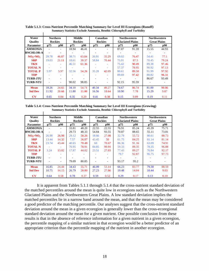
Table 5.1.3: Cross-Nutrient Percentile Matching Summary for Level III Ecoregions (Runoff)
p75 p90 p75 p90 p75 p90 p75 p90 p75 p90AMMONIA - - 18.94 46.41 - - 87.07 91.59 15.55 44.93
BNCHLOR-A - - - - - - - - - -NO3+NO2 46.87 63.84 35.29 76.47 77.1
SRP 21.11 39.37 70.44 87.5 79.24TKN - 61.36 - 90.49 97.46
TOTAL N - - - 78.95 97.13TOTAL P 5.97 54.26 42.09 89.58 97.92
TDP - - - 97.42 96.31
Mean 24.65 54.71 49.27 86.74 90.86Std Dev 20.68 11.00 18.64 7.78 9.87
CV 0.84 0.20 0.38 0.09 0.11
29.78 38.71 26.91 69.02 54.4119.03 18.61 58.84 75.91 70.45
- 46.51 - 75.42 89.38- - - 57.37 90.92
5.97 32.56 35.28 80.61 91.99- - - 89.69 88.82
TURB-JTU - - - - - - - - 86.67 93.49TURB-NTU - - 90.02 98.85 - - 92.15 95.59 - -
18.26 34.10 40.34 74.67 81.0011.92 11.80 16.56 10.90 15.29
0.65 0.35 0.41 0.15 0.19
Summary Statistics Exclude Ammonia, Benthic Chlorophyll and Turbidity
Water Quality
Parameter
Northern Middle Canadian Northwestern NorthwesternRockies Rockies Rockies Glaciated Plains Great Plains
Table 5.1.4: Cross-Nutrient Percentile Matching Summary for Level III Ecoregions (Growing)
p75 p90 p75 p90 p75 p90 p75 p90 p75 p90AMMONIA - - 33.81 48.20 22.55 22.55 76.91 85.24 45.39 75.71
BNCHLOR-A - - 29.73 48.33 54.84 93.55 70.87 88.65 55.11 73.81NO3+NO2 26.98 58.26 27.08 55.72 88.73
SRP 14.32 26.87 50 84.25 81.14TKN 43.44 70.48 70.67 91.16 74.91
TOTAL N - 78.91 90.91 89.35 96.88TOTAL P 13.02 44.02 27.03 89.27 92.17
TDP - - - 92.87 97.73
Mean 24.44 55.71 53.14 83.77 88.59Std Dev 14.15 20.80 27.86 14.04 9.03
CV 0.58 0.37 0.52 0.17 0.10
26.98 29.12 18.66 32.79 80.6113.44 7.57 43.45 61.75 81.1423.74 40.65 60 86.36 63.09
- 76.95 84.85 59.33 78.353.24 17.87 23.51 77.43 76.84
- - - 79.7 95.75TURB-JTU - - - - - - - - - -TURB-NTU - - 79.09 80.85 - - 93.17 95.2 - -
16.85 34.43 46.09 66.23 79.3010.75 26.79 27.23 19.48 10.44
0.64 0.78 0.59 0.29 0.13
Summary Statistics Exclude Ammonia, Benthic Chlorophyll and Turbidity
Water Quality
Parameter
Northern Middle Canadian Northwestern NorthwesternRockies Rockies Rockies Glaciated Plains Great Plains
It is apparent from Tables 5.1.1 through 5.1.4 that the cross-nutrient standard deviation of
the matched percentiles around the mean is quite low in ecoregions such as the Northwestern Glaciated Plains and the Northwestern Great Plains. A low standard deviation implies the matched percentiles lie in a narrow band around the mean, and that the mean may be considered a good predictor of the matching percentile. Our analyses suggest that the cross-nutrient standard deviation around the mean in a given ecoregion is generally lower than the cross-ecoregional standard deviation around the mean for a given nutrient. One possible conclusion from these results is that in the absence of reference information for a given nutrient in a given ecoregion, the percentile mapping of a similar nutrient in that ecoregion would be a better predictor of an appropriate criterion than the percentile mapping of the nutrient in another ecoregion.
18

5.2 Testing of Stratification Methodologies
Coarse-scale Stratifications for the General Population
Tables 5.2.1 through 5.2.4 report the results of the Kruskal Wallis test for between-strata differences in median nutrient concentrations for various coarse-scale stratification methodologies for the general population for a limited selection of nutrient parameters. These tests were performed on the median database only. These tables show that stratification by Omernik level III ecoregions consistently produce strata that differ from one another in terms of their median nutrient concentrations for all nutrients for all seasons. Geologic formation is also a significant coarse-scale stratification methodology. Grouped level III ecoregions and Strahler stream order are less consistently significant as course-scale stratifying methodologies.
Table 5.2.1 : Statistical Significance of Coarse Scale Stratifying Parameters (General Population, Median Data, All Seasons)
TKN TOTALN NO3+NO2 SRP TOTALP TDPGrouped Level III Ecoregions Y Y Y Y Y NLevel III Ecoregions Y Y Y Y Y YGeologic Formation Y Y Y Y Y NStrahler Stream Order Y Y Y N Y Y
"Y" indicates significant differences in median concentrations between different levels of the stratifying parameter (KW Test, 95% confidence level)"N" indicates absence of significant differences in median concentrations between different strata"-" indicates inadequate data
Nutrient GroupStratifying Parameter
Table 5.2.2 : Statistical Significance of Coarse Scale Stratifying Parameters(General Population, Median Data, Winter)
TKN TOTALN NO3+NO2 SRP TOTALP TDPGrouped Level III Ecoregions Y Y Y N Y YLevel III Ecoregions Y Y Y Y Y YGeologic Formation Y Y Y Y Y NStrahler Stream Order N Y N N N Y
"Y" indicates significant differences in median concentrations between different levels of the stratifying parameter (KW Test, 95% confidence level)"N" indicates absence of significant differences in median concentrations between different strata"-" indicates inadequate data
Nutrient GroupStratifying Parameter
19

Table 5.2.3 : Statistical Significance of Coarse Scale Stratifying Parameters(General Population, Median Data, Runoff)
TKN TOTALN NO3+NO2 SRP TOTALP TDPGrouped Level III Ecoregions Y Y Y N Y NLevel III Ecoregions Y Y Y Y Y NGeologic Formation Y Y Y Y Y NStrahler Stream Order Y N Y N Y N
"Y" indicates significant differences in median concentrations between different levels of the stratifying parameter (KW Test, 95% confidence level)"N" indicates absence of significant differences in median concentrations between different strata"-" indicates inadequate data
Nutrient GroupStratifying Parameter
Table 5.2.4 : Statistical Significance of Coarse Scale Stratifying Parameters(General Population, Median Data, Growing)
TKN TOTALN NO3+NO2 SRP TOTALP TDPGrouped Level III Ecoregions Y Y N N Y NLevel III Ecoregions Y Y Y Y Y YGeologic Formation Y Y Y Y Y NStrahler Stream Order Y Y Y N Y N
"Y" indicates significant differences in median concentrations between different levels of the stratifying parameter (KW Test, 95% confidence level)"N" indicates absence of significant differences in median concentrations between different strata"-" indicates inadequate data
Nutrient GroupStratifying Parameter
Course-Scale Stratifications for the Reference Population Tables 5.2.5 through 5.2.8 report the results of the Kruskal Wallis test for between-strata
differences in median nutrient concentrations for various coarse-scale stratification methodologies for the reference population for a limited selection of nutrient parameters. These tests were performed on the median database only.
It is apparent from these tables that none of the coarse-scale stratification methodologies
are effective for the Winter and Runoff seasons for the reference data. However, for the Growing season, and for all seasons together, stratification by Omernik level III ecoregions does produce strata that differ from one another in terms of their median nutrient concentrations for nearly all nutrient groupings.
20

Table 5.2.5 : Statistical Significance of Coarse Scale Stratifying Parameters (Reference Population, Median Data, All Seasons)
TKN TOTALN NO3+NO2 SRP TOTALP TDPGrouped Level III Ecoregions Y Y N N Y NLevel III Ecoregions Y Y Y Y Y NGeologic Formation Y Y N N Y NStrahler Stream Order N Y N N N N
"Y" indicates significant differences in median concentrations between different levels of the stratifying parameter (KW Test, 95% confidence level)"N" indicates absence of significant differences in median concentrations between different strata"-" indicates inadequate data
Nutrient GroupStratifying Parameter
Table 5.2.6 : Statistical Significance of Coarse Scale Stratifying Parameters (Reference Population, Median Data, Winter)
TKN TOTALN NO3+NO2 SRP TOTALP TDPGrouped Level III Ecoregions Y N N N Y NLevel III Ecoregions Y N N N N NGeologic Formation N N N N N NStrahler Stream Order N N N N N N
"Y" indicates significant differences in median concentrations between different levels of the stratifying parameter (KW Test, 95% confidence level)"N" indicates absence of significant differences in median concentrations between different strata"-" indicates inadequate data
Nutrient GroupStratifying Parameter
Table 5.2.7 : Statistical Significance of Coarse Scale Stratifying Parameters(Reference Population, Median Data, Runoff)
TKN TOTALN NO3+NO2 SRP TOTALP TDPGrouped Level III Ecoregions Y Y N N Y NLevel III Ecoregions Y N N N Y NGeologic Formation N N N N N NStrahler Stream Order Y N N N Y N
"Y" indicates significant differences in median concentrations between different levels of the stratifying parameter (KW Test, 95% confidence level)"N" indicates absence of significant differences in median concentrations between different strata"-" indicates inadequate data
Nutrient GroupStratifying Parameter
21

Table 5.2.8 : Statistical Significance of Coarse Scale Stratifying Parameters(Reference Population, Median Data, Growing)
TKN TOTALN NO3+NO2 SRP TOTALP TDPGrouped Level III Ecoregions Y Y N Y Y NLevel III Ecoregions Y Y Y Y Y NGeologic Formation Y Y N Y Y NStrahler Stream Order N Y N N N N
"Y" indicates significant differences in median concentrations between different levels of the stratifying parameter (KW Test, 95% confidence level)"N" indicates absence of significant differences in median concentrations between different strata"-" indicates inadequate data
Nutrient GroupStratifying Parameter
Fine-scale Sub-stratifications for the General Population Tables 5.2.9 through 5.2.12 report the results of post-ANOVA Wald tests used to verify
the statistical significance of various sub-stratification methodologies within coarse-scale strata for the general population for a limited selection of nutrient parameters. These tests were performed on the median database only. These tables indicate that sub-stratification by Omernik level IV ecoregions is consistently an improvement over stratification by Omernik level III ecoregions for all seasons combined and for specific seasons. However, sub-stratifications based on geological formation and Strahler stream order within Omernik level III ecoregions are also significant. To decide between these competing sub-stratification methodologies, ICF recommends choosing the one that a priori creates zones most similar in terms of composite physical, ecological and hydrogeological parameters. In this respect, Omernik level IV ecoregions seems to be a superior sub-stratification methodology to geological formation and Strahler stream order, which do not control for ecological effects and which group widely dispersed areas together.
As an additional but secondary basis for deciding between competing stratification
methodologies, it is possible to compare the performance of each methodology in terms of total variance explained (as measured by the adjusted R2) and the mean coefficient of variance. Such a comparison is admissible in this circumstance, because these sub-stratification methodologies divide the state into roughly equal numbers of zones. On the basis of these measures of variance, the sub-stratification based on Omernik level IV ecoregions generally outperforms the others. However, statistical significance and expert judgment are the best basis for deciding on a stratification methodology.
The analysis shows that even finer sub-stratification of Omernik level IV ecoregions by
Strahler stream order produces statistically significant results. However, this level of stratification would fragment the state into too many nutrient zones to be practically useful. Also, given the small number of observations, especially reference observations, in each of the resulting nutrient zones, this level of stratification would result in excessively wide confidence intervals around the criteria.
22
23
Fine-scale Sub-stratifications for the Reference Population Tables 5.2.13 through 5.2.16 report the results of post-ANOVA Wald tests used to verify
the statistical significance of various sub-stratification methodologies for coarse-scale strata for the reference population for a limited selection of nutrient parameters. These tests were performed on the median database only.
At the all-season level, sub-stratification by Omernik level IV ecoregions is consistently
an improvement over stratification by Omernik level III ecoregions. The other sub-stratification methods do not show statistically significant results. However, sample size was limited at this level of stratification for the reference population and the power of these tests is likely to be low.

Table 5.2.9 : Statistical Significance of Fine Scale Stratifying Parameters (General Population, Median Data, All Seasons)
Significance Adjusted R2 Significance Adjusted R2 Significance Adjusted R2 Significance Adjusted R2Level III Ecoregions Level IV Ecoregions Y 0.3681 Y 0.6607 Y 0.1176 Y 0.2708Level III Ecoregions Strahler Stream Order Y 0.2116 Y 0.5662 Y 0.0664 Y 0.1786Level III Ecoregions Geologic Formation Y 0.2474 Y 0.58 Y 0.0928 Y 0.1588Level IV Ecoregions Strahler Stream Order Y 0.409 Y 0.7507 Y 0.1569 Y 0.345
"Y" indicates the sub-stratification is significant (post-ANOVA Wald test, 95% confidence level)"N" indicates the sub-stratification is not significant"-" indicates inadequate data
Nutrient GroupStratifying Parameter Sub-Stratifying Parameter TKN TOTALN SRP TOTALP
Table 5.2.10: Statistical Significance of Fine Scale Stratifying Parameters (General Population, Median Data, Winter)
Significance Adjusted R2 Significance Adjusted R2 Significance Adjusted R2 Significance Adjusted R2Level III Ecoregions Level IV Ecoregions Y 0.4073 Y 0.6716 Y 0.1069 Y 0.2271Level III Ecoregions Strahler Stream Order Y 0.2225 Y 0.5122 Y 0.0455 Y 0.132Level III Ecoregions Geologic Formation Y 0.2188 Y 0.5957 Y 0.0696 Y 0.1118Level IV Ecoregions Strahler Stream Order Y 0.5271 Y 0.7333 N 0.134 Y 0.277
"Y" indicates the sub-stratification is significant (post-ANOVA Wald test, 95% confidence level)"N" indicates the sub-stratification is not significant"-" indicates inadequate data
Stratifying Parameter Sub-Stratifying ParameterNutrient Group
TKN TOTALN SRP TOTALP
24

Table 5.2.11 : Statistical Significance of Fine Scale Stratifying Parameters (General Population, Median Data, Runoff)
Significance Adjusted R2 Significance Adjusted R2 Significance Adjusted R2 Significance Adjusted R2Level III Ecoregions Level IV Ecoregions Y 0.4175 Y 0.7652 Y 0.1532 Y 0.2871Level III Ecoregions Strahler Stream Order Y 0.2126 N 0.5993 Y 0.0796 Y 0.195Level III Ecoregions Geologic Formation Y 0.2513 Y 0.7037 Y 0.0824 Y 0.1426Level IV Ecoregions Strahler Stream Order Y 0.48 N 0.8052 Y 0.1902 Y 0.3599
"Y" indicates the sub-stratification is significant (post-ANOVA Wald test, 95% confidence level)"N" indicates the sub-stratification is not significant"-" indicates inadequate data
Nutrient GroupStratifying Parameter Sub-Stratifying Parameter TKN TOTALN SRP TOTALP
Table 5.2.12 : Statistical Significance of Fine Scale Stratifying Parameters (General Population, Median Data, Growing)
Significance Adjusted R2 Significance Adjusted R2 Significance Adjusted R2 Significance Adjusted R2Level III Ecoregions Level IV Ecoregions Y 0.4277 Y 0.7002 Y 0.1428 Y 0.2991Level III Ecoregions Strahler Stream Order Y 0.2411 Y 0.5715 Y 0.0888 Y 0.2211Level III Ecoregions Geologic Formation Y 0.245 Y 0.6232 Y 0.0904 Y 0.196Level IV Ecoregions Strahler Stream Order Y 0.4791 Y 0.7395 Y 0.2208 Y 0.383
"Y" indicates the sub-stratification is significant (post-ANOVA Wald test, 95% confidence level)"N" indicates the sub-stratification is not significant"-" indicates inadequate data
Nutrient GroupStratifying Parameter Sub-Stratifying Parameter TKN TOTALN SRP TOTALP
25

Table 5.2.13 : Statistical Significance of Fine Scale Stratifying Parameters (Reference Population, Median Data, All Seasons)
Significance Adjusted R2 Significance Adjusted R2 Significance Adjusted R2 Significance Adjusted R2Level III Ecoregions Level IV Ecoregions Y 0.6416 Y 0.6855 Y 0.5653 Y 0.5477Level III Ecoregions Strahler Stream Order N 0.5163 Y 0.6746 N 0.2192 N 0.4177Level III Ecoregions Geologic Formation N 0.6128 N 0.6687 N 0.1992 Y 0.5281Level IV Ecoregions Strahler Stream Order N 0.679 N 0.7021 N 0.599 Y 0.6338
"Y" indicates the sub-stratification is significant (post-ANOVA Wald test, 95% confidence level)"N" indicates the sub-stratification is not significant"-" indicates inadequate data
Sub-Stratifying ParameterStratifying ParameterNutrient Group
TKN TOTALN SRP TOTALP
Table 5.2.14 : Statistical Significance of Fine Scale Stratifying Parameters (Reference Population, Median Data, Winter)
Significance Adjusted R2 Significance Adjusted R2 Significance Adjusted R2 Significance Adjusted R2Level III Ecoregions Level IV Ecoregions N 0.421 - - N 0.5171 Y 0.8828Level III Ecoregions Strahler Stream Order N 0.6487 N 0.6743 N 0.0842 N 0.2366Level III Ecoregions Geologic Formation N 0.5989 N -0.4625 N -0.0044 N 0.3818Level IV Ecoregions Strahler Stream Order N 0.5419 - - N 0.3561 N 0.8929
"Y" indicates the sub-stratification is significant (post-ANOVA Wald test, 95% confidence level)"N" indicates the sub-stratification is not significant"-" indicates inadequate data
Sub-Stratifying ParameterStratifying ParameterNutrient Group
TKN TOTALN SRP TOTALP
26

Table 5.2.15 : Statistical Significance of Fine Scale Stratifying Parameters (Reference Population, Median Data, Runoff)
Significance Adjusted R2 Significance Adjusted R2 Significance Adjusted R2 Significance Adjusted R2Level III Ecoregions Level IV Ecoregions N 0.7344 N 0.6694 N 0.3725 N 0.6354Level III Ecoregions Strahler Stream Order N 0.6749 N 0.4958 N 0.1763 N 0.6764Level III Ecoregions Geologic Formation Y 0.7608 N 0.5785 N 0.1222 N 0.6177Level IV Ecoregions Strahler Stream Order N 0.8063 N 0.4958 Y 0.8623 N 0.6494
"Y" indicates the sub-stratification is significant (post-ANOVA Wald test, 95% confidence level)"N" indicates the sub-stratification is not significant"-" indicates inadequate data
Sub-Stratifying ParameterStratifying ParameterNutrient Group
TKN TOTALN SRP TOTALP
27
Table 5.2.16 : Statistical Significance of Fine Scale Stratifying Parameters (Reference Population, Median Data, Growing)
Significance Adjusted R2 Significance Adjusted R2 Significance Adjusted R2 Significance Adjusted R2Level III Ecoregions Level IV Ecoregions N 0.6386 N 0.7197 Y 0.613 Y 0.5586Level III Ecoregions Strahler Stream Order N 0.5884 N 0.8079 Y 0.3456 N 0.4449Level III Ecoregions Geologic Formation Y 0.6662 Y 0.8074 N 0.2519 Y 0.5821Level IV Ecoregions Strahler Stream Order N 0.6654 N 0.783 N 0.5934 N 0.6401
"Y" indicates the sub-stratification is significant (post-ANOVA Wald test, 95% confidence level)"N" indicates the sub-stratification is not significant"-" indicates inadequate data
Sub-Stratifying ParameterStratifying ParameterNutrient Group
TKN TOTALN SRP TOTALP

28
5.3 Computation of Measures of Variation for Stratification Methodologies
In order to assess how well the various stratification methodologies perform in explaining nutrient concentration variability, we computed the mean coefficient of variation (MCV) and the coefficient of efficiency (COE).
As described in Section 4, the MCV and the COE should not be used to compare
stratification methodologies that create widely differing numbers of strata. This is because both measures are likely to improve as the dataset is increasingly partitioned and as fewer numbers of observations become available in each stratum.
The measures may be used, however, in combination with the tests of significance and
theoretical considerations described in Section 5.2, to compare stratifications and sub-stratifications that partition the state into similar numbers of strata. They are also useful in identifying seasons with high variance in nutrient concentrations. All COEs in Tables 5.3.1 through 5.3.16 are reported for log-transformed data.
Course-scale Stratifications for the General Population Tables 5.3.1 through 5.3.4 report the MCV and COE for selected coarse-scale
stratifications in the general population for a selection of nutrient groupings by season. These tables indicate that the stratification methodologies considered are more successful in explaining variance for nitrogen group nutrients than for phosphorus groups. This is consistent with the findings in Robertson, et al. (2001). However, the values of the MCVs computed in this analysis are higher than those reported in that paper.8 It is also notable that the stratification methodologies have the most explanatory power in the Winter season.
8 The higher values observed in the general population analysis (compared to Robertson (2001)) may be the result of using a database that was not specifically selected to exclude particular sites or observations except those that did not pass the QC measures used to screen the data. The stratification methodologies used in this analysis are mainly intended to capture factors that contribute to natural nutrient loadings. This is evident in the better performance of the stratification methodologies in the designated reference data. It should also be noted that the data used in the general population analysis spanned over 40 years. Partitioning the data by time periods (e.g. 1990s only) may potentially reduce variability further. The current analysis used data that spanned both wet and dry climatic cycles which necessitated using multiple-decade data. Reducing the data to a given decade could reduce noise, especially if all the data come from a dry cycle, for example, but would be less representative of the complete recent climatic record.

Table 5.3.1 : MCV Summary by Coarse Scale Stratifying Parameter (General Population, Median Data, All Seasons)
MCV COE MCV COE MCV COE MCV COEGrouped Level III Ecoregions 3.95 0.16 2.12 0.52 5.17 0.004 5.46 0.09Level III Ecoregions 3.82 0.17 1.96 0.53 3.94 0.05 5.23 0.12Level IV Ecoregions 1.72 0.39 1.57 0.71 2.9 0.15 3.59 0.29Geologic Formation 2.54 0.14 2.23 0.34 3.86 0.06 5.26 0.08Strahler Stream Order 2.79 0.04 1.83 0.05 4.5 0.003 5.49 0.03
MCV=Mean Coefficient of VariationCOE= Coefficient of Efficiency
Nutrient and Measure of VariationStratifying Parameter TKN TOTALN SRP TOTALP
Table 5.3.2: MCV Summary by Coarse Scale Stratifying Parameter (General Population, Median Data, Winter)
MCV COE MCV COE MCV COE MCV COEGrouped Level III Ecoregions 1.84 0.12 0.87 0.45 5.3 0.0007 4.09 0.01Level III Ecoregions 1.85 0.15 0.82 0.47 3.73 0.04 3.44 0.07Level IV Ecoregions 1.13 0.44 0.61 0.72 2.45 0.15 2.44 0.27Geologic Formation 1.35 0.17 0.91 0.29 3.98 0.04 3.22 0.04Strahler Stream Order 1.37 0.01 0.86 0.09 3.99 0.01 3.37 0.01
MCV=Mean Coefficient of VariationCOE= Coefficient of Efficiency
Nutrient and Measure of VariationStratifying Parameter TKN TOTALN SRP TOTALP
29

Table 5.3.3 : MCV Summary by Coarse Scale Stratifying Parameter (General Population, Median Data, Runoff)
MCV COE MCV COE MCV COE MCV COEGrouped Level III Ecoregions 4.06 0.16 0.92 0.59 4.02 0.0001 5.12 0.07Level III Ecoregions 3.91 0.18 0.89 0.6 3.52 0.05 4.97 0.1Level IV Ecoregions 1.47 0.45 0.69 0.81 2.09 0.2 3.05 0.32Geologic Formation 2.54 0.15 0.93 0.33 3.1 0.05 4.35 0.09Strahler Stream Order 2.44 0.04 0.87 0.07 3.07 0.004 3.71 0.07
MCV=Mean Coefficient of VariationCOE= Coefficient of Efficiency
Nutrient and Measure of VariationStratifying Parameter TKN TOTALN SRP TOTALP
30
Table 5.3.4 : MCV Summary by Coarse Scale Stratifying Parameter (General Population, Median Data, Growing)
MCV COE MCV COE MCV COE MCV COEGrouped Level III Ecoregions 1.6 0.17 2.31 0.54 3.8 0.00003 4.66 0.1Level III Ecoregions 1.57 0.18 2.08 0.56 3.32 0.06 4.37 0.14Level IV Ecoregions 1.12 0.45 1.44 0.75 1.57 0.19 2.04 0.33Geologic Formation 1.4 0.12 2.41 0.31 2.44 0.06 4.65 0.1Strahler Stream Order 1.33 0.05 2.02 0.08 2.6 0.007 4.76 0.03
MCV=Mean Coefficient of VariationCOE= Coefficient of Efficiency
Stratifying ParameterNutrient and Measure of Variation
TKN TOTALN SRP TOTALP

31
Coarse-scale Stratifications for the Reference Population Tables 5.3.5 through 5.3.8 report the MCV and COE for selected coarse-scale
stratifications in the reference population for a selection of nutrient groupings by season. The stratification methodologies show considerably lower variance for these data than for the general population. The tables also indicate that the stratification methodologies considered are more successful in explaining variance for nitrogen group nutrients than for phosphorus groups. As was evident for the general population, the stratification methodologies have the most explanatory power in the Winter season. The Growing season appears to be the most noisy.

Table 5.3.5 : MCV Summary by Coarse Scale Stratifying Parameter (Reference Population, Median Data, All Seasons)
MCV COE MCV COE MCV COE MCV COEGrouped Level III Ecoregions 2.01 0.49 2.18 0.51 0.76 0.07 2.27 0.28Level III Ecoregions 1.57 0.57 1.5 0.61 1.69 0.19 1.73 0.44Level IV Ecoregions 0.76 0.79 0.7 0.83 0.9 0.77 1.15 0.7Geologic Formation 1.14 0.56 1.04 0.57 1.55 0.26 1.75 0.35Strahler Stream Order 1.36 0.14 1.45 0.31 1.54 0.04 1.84 0.1
MCV=Mean Coefficient of VariationCOE= Coefficient of Efficiency
Stratifying ParameterNutrient and Measure of Variation
TKN TOTALN SRP TOTALP
Table 5.3.6 : MCV Summary by Coarse Scale Stratifying Parameter (Reference Population, Median Data, Winter)
MCV COE MCV COE MCV COE MCV COEGrouped Level III Ecoregions 0.53 0.62 0.78 0.06 1.26 0.2 0.9 0.19Level III Ecoregions 0.54 0.63 0.89 0.06 1.04 0.4 0.78 0.42Level IV Ecoregions 0.55 0.74 0 1 0.4 0.88 0.25 0.97Geologic Formation 0.47 0.78 0.56 0.37 1.23 0.19 1.1 0.15Strahler Stream Order 0.48 0.79 0.67 0.66 0.96 0.6 0.69 0.43
MCV=Mean Coefficient of VariationCOE= Coefficient of Efficiency
Stratifying ParameterNutrient and Measure of Variation
TKN TOTALN SRP TOTALP
32
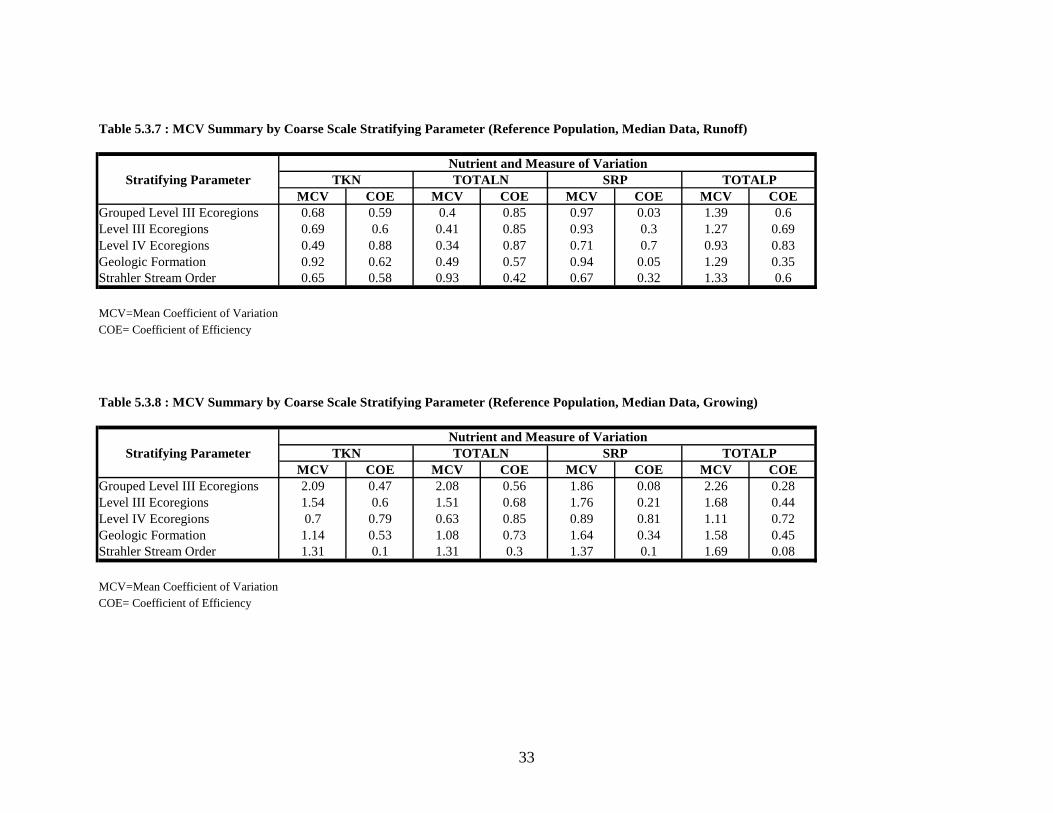
Table 5.3.7 : MCV Summary by Coarse Scale Stratifying Parameter (Reference Population, Median Data, Runoff)
MCV COE MCV COE MCV COE MCV COEGrouped Level III Ecoregions 0.68 0.59 0.4 0.85 0.97 0.03 1.39 0.6Level III Ecoregions 0.69 0.6 0.41 0.85 0.93 0.3 1.27 0.69Level IV Ecoregions 0.49 0.88 0.34 0.87 0.71 0.7 0.93 0.83Geologic Formation 0.92 0.62 0.49 0.57 0.94 0.05 1.29 0.35Strahler Stream Order 0.65 0.58 0.93 0.42 0.67 0.32 1.33 0.6
MCV=Mean Coefficient of VariationCOE= Coefficient of Efficiency
Stratifying ParameterNutrient and Measure of Variation
TKN TOTALN SRP TOTALP
33
Table 5.3.8 : MCV Summary by Coarse Scale Stratifying Parameter (Reference Population, Median Data, Growing)
MCV COE MCV COE MCV COE MCV COEGrouped Level III Ecoregions 2.09 0.47 2.08 0.56 1.86 0.08 2.26 0.28Level III Ecoregions 1.54 0.6 1.51 0.68 1.76 0.21 1.68 0.44Level IV Ecoregions 0.7 0.79 0.63 0.85 0.89 0.81 1.11 0.72Geologic Formation 1.14 0.53 1.08 0.73 1.64 0.34 1.58 0.45Strahler Stream Order 1.31 0.1 1.31 0.3 1.37 0.1 1.69 0.08
MCV=Mean Coefficient of VariationCOE= Coefficient of Efficiency
Stratifying ParameterNutrient and Measure of Variation
TKN TOTALN SRP TOTALP

34
Fine-scale Sub-stratifications for the General Population Tables 5.3.9 through 5.3.12 report the MCV and COE for selected fine-scale
stratifications in the general population for a selection of nutrient groupings by season. These tables indicate a considerable improvement in the measures of variance with increasing sub-stratification. However, as explained earlier, this improvement may partly be the result of a fewer number of observations contributing to each stratum.

Table 5.3.9 : MCV Summary by Fine Scale Stratifying Parameter (General Population, Median Data, All Seasons)
MCV COE MCV COE MCV COE MCV COEGrouped Level III Ecoregions Strahler Stream Order 2.52 0.2 1.57 0.57 3.97 0.03 4.07 0.133Level III Ecoregions Strahler Stream Order 2.1 0.23 1.28 0.61 2.42 0.09 0.46 0.2Level IV Ecoregions Strahler Stream Order 1.08 0.5 0.7 0.84 1.54 0.3 1.73 0.44
MCV=Mean Coefficient of VariationCOE= Coefficient of Efficiency
Nutrient and Measure of VariationTKN TOTALN SRP TOTALPStratifying Parameter Sub Stratifying Parameter
Table 5.3.10 : MCV Summary by Fine Scale Stratifying Parameter (General Population, Median Data, Winter)
MCV COE MCV COE MCV COE MCV COEGrouped Level III Ecoregions Strahler Stream Order 1.17 0.2 0.69 0.54 3.78 0.03 2.71 0.08Level III Ecoregions Strahler Stream Order 1.02 0.26 0.65 0.57 2.08 0.09 1.71 0.17Level IV Ecoregions Strahler Stream Order 0.69 0.65 0.47 0.83 1.3 0.34 1.05 0.44
MCV=Mean Coefficient of VariationCOE= Coefficient of Efficiency
Stratifying Parameter Sub Stratifying ParameterNutrient and Measure of Variation
TKN TOTALN SRP TOTALP
35

Table 5.3.11 : MCV Summary by Fine Scale Stratifying Parameter (General Population, Median Data, Runoff)
MCV COE MCV COE MCV COE MCV COEGrouped Level III Ecoregions Strahler Stream Order 2 0.19 0.87 0.64 2.53 0.02 3.18 0.16Level III Ecoregions Strahler Stream Order 1.53 0.25 0.81 0.66 1.87 0.12 2.63 0.23Level IV Ecoregions Strahler Stream Order 0.87 0.61 0.5 0.87 1.07 0.38 1.36 0.5
MCV=Mean Coefficient of VariationCOE= Coefficient of Efficiency
Stratifying Parameter Sub Stratifying ParameterNutrient and Measure of Variation
TKN TOTALN SRP TOTALP
36
Table 5.3.12 : MCV Summary by Fine Scale Stratifying Parameter (General Population, Median Data, Growing)
MCV COE MCV COE MCV COE MCV COEGrouped Level III Ecoregions Strahler Stream Order 1.2 0.23 1.71 0.58 1.99 0.03 3 0.16Level III Ecoregions Strahler Stream Order 1.13 0.26 1.36 0.62 1.71 0.12 2.35 0.24Level IV Ecoregions Strahler Stream Order 0.77 0.59 0.7 0.85 1.05 0.39 1.23 0.51
MCV=Mean Coefficient of VariationCOE= Coefficient of Efficiency
Stratifying Parameter Sub Stratifying ParameterNutrient and Measure of Variation
TKN TOTALN SRP TOTALP

37
Fine-scale Sub-stratification for the Reference Population Tables 5.3.13 through 5.3.16 report the MCV and COE for selected fine-scale
stratifications in the reference population for a selection of nutrient groupings by season. These tables indicate an even greater improvement in the measures of variance with increasing sub-stratification for the reference population. However, as explained earlier, these effects may be the result of a fewer number of observations contributing to each stratum.

Table 5.3.13 : MCV Summary by Fine Scale Stratifying Parameter (Reference Population, Median Data, All Seasons)
MCV COE MCV COE MCV COE MCV COEGrouped Level III Ecoregions Strahler Stream Order 1.28 0.55 1.51 0.59 1.21 0.26 1.7 0.36Level III Ecoregions Strahler Stream Order 1.07 0.64 1.03 0.78 1.01 0.43 1.34 0.52Level IV Ecoregions Strahler Stream Order 0.58 0.88 0.54 0.89 0.51 0.85 0.91 0.82
MCV=Mean Coefficient of VariationCOE= Coefficient of Efficiency
Stratifying Parameter Sub Stratifying ParameterNutrient and Measure of Variation
TKN TOTALN SRP TOTALP
Table 5.3.14 : MCV Summary by Fine Scale Stratifying Parameter (Reference Population, Median Data, Winter)
MCV COE MCV COE MCV COE MCV COEGrouped Level III Ecoregions Strahler Stream Order 0.44 0.81 0.38 0.89 0.94 0.62 0.71 0.47Level III Ecoregions Strahler Stream Order 0.44 0.81 0.37 0.89 0.89 0.66 0.48 0.7Level IV Ecoregions Strahler Stream Order 0.47 0.83 0 1 0.4 0.88 0.18 0.98
MCV=Mean Coefficient of VariationCOE= Coefficient of Efficiency
Sub Stratifying ParameterStratifying ParameterNutrient and Measure of Variation
TKN TOTALN SRP TOTALP
38

Table 5.3.15 : MCV Summary by Fine Scale Stratifying Parameter (Reference Population, Median Data, Runoff)
MCV COE MCV COE MCV COE MCV COEGrouped Level III Ecoregions Strahler Stream Order 0.52 0.82 0.35 0.89 0.65 0.47 1.08 0.78Level III Ecoregions Strahler Stream Order 0.55 0.84 0.33 0.9 0.79 0.61 0.93 0.82Level IV Ecoregions Strahler Stream Order 0.31 0.95 0.33 0.9 0.28 0.96 0.75 0.89
MCV=Mean Coefficient of VariationCOE= Coefficient of Efficiency
Sub Stratifying ParameterStratifying ParameterNutrient and Measure of Variation
TKN TOTALN SRP TOTALP
39
Table 5.3.16 : MCV Summary by Fine Scale Stratifying Parameter (Reference Population, Median Data, Growing)
MCV COE MCV COE MCV COE MCV COEGrouped Level III Ecoregions Grouped Strahler Stream Order 1.26 0.56 1.29 0.66 1.04 0.41 1.61 0.73Level III Ecoregions Grouped Strahler Stream Order 1.01 0.72 0.9 0.88 0.78 0.56 1.24 0.57Level IV Ecoregions Grouped Strahler Stream Order 0.52 0.89 0.52 0.92 0.53 0.85 0.78 0.84
MCV=Mean Coefficient of VariationCOE= Coefficient of Efficiency
Stratifying Parameter Sub Stratifying ParameterNutrient and Measure of Variation
TKN TOTALN SRP TOTALP
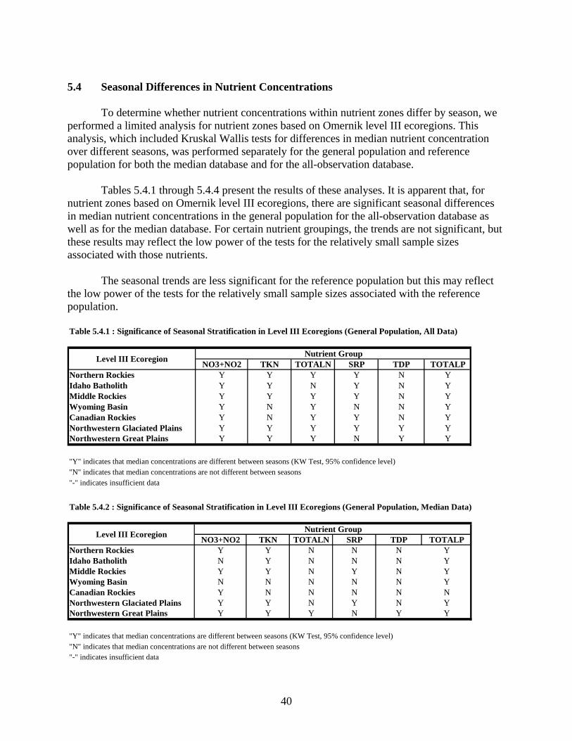
5.4 Seasonal Differences in Nutrient Concentrations
To determine whether nutrient concentrations within nutrient zones differ by season, we performed a limited analysis for nutrient zones based on Omernik level III ecoregions. This analysis, which included Kruskal Wallis tests for differences in median nutrient concentration over different seasons, was performed separately for the general population and reference population for both the median database and for the all-observation database.
Tables 5.4.1 through 5.4.4 present the results of these analyses. It is apparent that, for nutrient zones based on Omernik level III ecoregions, there are significant seasonal differences in median nutrient concentrations in the general population for the all-observation database as well as for the median database. For certain nutrient groupings, the trends are not significant, but these results may reflect the low power of the tests for the relatively small sample sizes associated with those nutrients.
The seasonal trends are less significant for the reference population but this may reflect
the low power of the tests for the relatively small sample sizes associated with the reference population. Table 5.4.1 : Significance of Seasonal Stratification in Level III Ecoregions (General Population, All Data)
NO3+NO2 TKN TOTALN SRP TDP TOTALPNorthern Rockies Y Y Y Y N YIdaho Batholith Y Y N Y N YMiddle Rockies Y Y Y Y N YWyoming Basin Y N Y N N YCanadian Rockies Y N Y Y N YNorthwestern Glaciated Plains Y Y Y Y Y YNorthwestern Great Plains Y Y Y N Y Y
"Y" indicates that median concentrations are different between seasons (KW Test, 95% confidence level)"N" indicates that median concentrations are not different between seasons"-" indicates insufficient data
Nutrient GroupLevel III Ecoregion
Table 5.4.2 : Significance of Seasonal Stratification in Level III Ecoregions (General Population, Median Data)
NO3+NO2 TKN TOTALN SRP TDP TOTALPNorthern Rockies Y Y N N N YIdaho Batholith N Y N N N YMiddle Rockies Y Y N Y N YWyoming Basin N N N N N YCanadian Rockies Y N N N N NNorthwestern Glaciated Plains Y Y N Y N YNorthwestern Great Plains Y Y Y N Y Y
"Y" indicates that median concentrations are different between seasons (KW Test, 95% confidence level)"N" indicates that median concentrations are not different between seasons"-" indicates insufficient data
Nutrient GroupLevel III Ecoregion
40

Table 5.4.3 : Significance of Seasonal Stratification in Level III Ecoregions (Reference Population, All Data)
NO3+NO2 TKN TOTALN SRP TDP TOTALPNorthern Rockies Y N N N - NIdaho Batholith N N N - - NMiddle Rockies Y Y N Y - YWyoming Basin - - - - - -Canadian Rockies Y N N N - YNorthwestern Glaciated Plains Y N N N N YNorthwestern Great Plains Y N N N N Y
"Y" indicates that median concentrations are different between seasons (KW Test, 95% confidence level)"N" indicates that median concentrations are not different between seasons"-" indicates insufficient data
Nutrient GroupLevel III Ecoregion
Table 5.4.4: Significance of Seasonal Stratification in Level III Ecoregions (Reference Population, Median Data)
NO3+NO2 TKN TOTALN SRP TDP TOTALPNorthern Rockies Y N N N - NIdaho Batholith N N N - NMiddle Rockies N N N N - NWyoming Basin - - - - NCanadian Rockies N N N N - NNorthwestern Glaciated Plains N N N N N NNorthwestern Great Plains N N N N N N
"Y" indicates that median concentrations are different between seasons (KW Test, 95% confidence level)"N" indicates that median concentrations are not different between seasons"-" indicates insufficient data
Nutrient GroupLevel III Ecoregion
5.5 Distribution of Stream Order in the Reference and General Population
In order to assess whether the distributions of stream orders in the reference and general populations were significantly different, we performed a limited analysis for nutrient zones based on Omernik level III ecoregions. The analysis, which included the Pearson Chi-square test, was performed separately at the all-observation level and at the station level for all seasons only.
Tables 5.5.1 and 5.5.2 present the results of these analyses. It is apparent that there are
significant differences in stream order distributions between the reference and general population for the all-observation database. The trend is less significant at the station level, in which each station contributes a single observation for each nutrient. The observed difference in trends between the all-observation database and the median database is because certain stations contribute substantially more observations than others. The statistically significant difference in stream order distributions between the reference and general population for the all-observation database implies that standards based on the reference population distributions in the all-observation database may be overly or insufficiently conservative, depending on whether lower order streams are over or under-represented in the reference population compared to the general population. The fact that the differences in stream order distribution between the general and
41

reference population are less pronounced in the median database implies that standards based on the reference population in the median database are less likely to be biased in this regard. However, relatively low sample size in the median database may have resulted in statistical tests with low power in some cases. Ideally, regulators should also ensure that the distribution of stream order in the general population is balanced and appropriately representative of each nutrient zone.
Table 5.5.1: Stream Order Distribution in Level III Ecoregions (General v Ref Population, All Data)
NO3+NO2 TKN TOTALN SRP TDP TOTALPNorthern Rockies Y Y Y Y - YIdaho Batholith N N - - - NMiddle Rockies Y Y Y Y - YWyoming Basin - - - - - -Canadian Rockies Y Y Y Y - YNorthwestern Glaciated Plains Y Y Y Y Y YNorthwestern Great Plains Y Y Y Y Y Y
"Y" indicates differences between stream order distribution in the reference and general population (Pearson Chi Square, 95%)"N" indicates stream order distributions are not different between the reference and general population"-" indicates insufficient data
Nutrient GroupLevel III Ecoregion
Table 5.5.2: Stream Order Distribution in Level III Ecoregions (General v Ref Population, Station Data)
NO3+NO2 TKN TOTALN SRP TDP TOTALPNorthern Rockies N N N N - NIdaho Batholith N N - - - NMiddle Rockies Y Y N Y - NWyoming Basin - - - - - -Canadian Rockies N N N N - NNorthwestern Glaciated Plains Y Y N Y N YNorthwestern Great Plains N N N N N N
"Y" indicates differences between stream order distribution in the reference and general population (Pearson Chi Square, 95%)"N" indicates stream order distributions are not different between the reference and general population"-" indicates insufficient data
Nutrient GroupLevel III Ecoregion
5.6 General Conclusions The preceding analyses suggest the following general conclusions:
Percentile mapping trends between the reference and general population do not show pronounced seasonal differences (based on the analysis for Omernik level III ecoregions);
Omernik level IV ecoregions constitute a statistically significant parameter for stratifying
the state for most nutrients in most seasons for both the general and reference population;
42
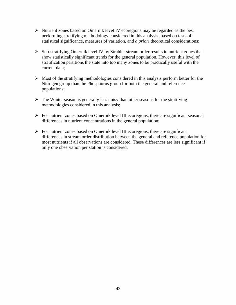
Nutrient zones based on Omernik level IV ecoregions may be regarded as the best performing stratifying methodology considered in this analysis, based on tests of statistical significance, measures of variation, and a priori theoretical considerations;
Sub-stratifying Omernik level IV by Strahler stream order results in nutrient zones that
show statistically significant trends for the general population. However, this level of stratification partitions the state into too many zones to be practically useful with the current data;
Most of the stratifying methodologies considered in this analysis perform better for the
Nitrogen group than the Phosphorus group for both the general and reference populations;
The Winter season is generally less noisy than other seasons for the stratifying
methodologies considered in this analysis;
For nutrient zones based on Omernik level III ecoregions, there are significant seasonal differences in nutrient concentrations in the general population;
For nutrient zones based on Omernik level III ecoregions, there are significant
differences in stream order distribution between the general and reference population for most nutrients if all observations are considered. These differences are less significant if only one observation per station is considered.
43
6. Literature Cited Cohen, J., 2005, Personal communication between Jonathan Cohen, Statistician, ICF Consulting, and Arun Varghese, Senior Associate, ICF Consulting, June 2, 2005. EPA, 2000, Nutrient Criteria Technical Guidance Manual, U.S. EPA, Office of Water, Document Number EPA-822-B-00-002, July 2000. ICF, 2004a. “Montana Rivers and Streams Reference-to-Whole-Population Percentile Mapping for Selected Water Quality Parameters – Final Report,” Memorandum to Dr. Michael Suplee, Montana Department of Environmental Quality, from Arun Varghese and Joshua Cleland, ICF Consulting, November 22, 2004. ICF, 2004b. “Stratification of Algae and Nutrient Data of Montana Rivers and Streams to Assist in the Development of Numeric Standards – Final Report,” Memorandum to Dr. Michael Suplee, Montana Department of Environmental Quality, from Arun Varghese and Joshua Cleland, ICF Consulting, July 13, 2004. MT DEQ, 2005. “Identification and Assessment of Montana Reference Streams: A Follow-up and Expansion of the 1992 Benchmark Biology Study”, Suplee, M., Sada de Suplee R., Feldman, D., Laidlaw, T. Legates, D.R. and McCabe, G.J. “Evaluating the Use of “Goodness of Fit” Measures in Hydrologic and Hydroclimatic Model Validation”, Water Resources Research, 1999, 35:233-241 Luce, W., 2005. Personal communication between Wendy Luce, Analytic Chemist, ICF Consulting, and Arun Varghese, Senior Associate, ICF Consulting, May 5, 2005. Robertson, D.M., Saad, A.S., Wieben, A.M., 2001. “An Alternative Regionalization Scheme for Defining Nutrient Criteria for Rivers and Streams.” U.S. Geological Survey, Middleton, WI. Water-Resources Investigations Report 01–4073. 2001. Siegel, S., & Castellan, N. J., Jr., 1988. Nonparametric Statistics for the Behavioural Sciences (2nd ed.). McGraw-Hill Publishing, New York. Statacorp. 2001. Stata Reference Manual, Stata Press, College Station, Texas.
44
APPENDIX A
WATER QUALITY DATA GROUPING METHODOLOGY
Prepared by: Dr. Michael Suplee, MT DEQ
Updated: May 16, 2005
Organization of Nutrient, Benthic Chlorophyll a and Turbidity data from NEW, Legacy, and non-STORET Databases
The organizational objective outlined herein was to group analytical measurements together that are fundamentally equivalent, while at the same time avoiding double-counts in cases where an agency may have measured two or more closely related parameters from the same sample. The approach was undertaken in a series of steps as follows:
1. The different analytical measurements (e.g. total nitrate, dissolved nitrate, total phosphorus) were identified in the database, checked against STORET and other records to determine what they actually measured, and then organized into groups. The groups (e.g., total N group, soluble reactive phosphorus group) were composed of similar measurements that fundamentally measured the same thing.
2. For each group, a series of exploratory queries were made in the databases, by
agency, to ascertain if the various analytical measurements within the group were derived from the same sample. In cases where this occurred, only one of the analytical measurements was retained for that particular agency. Entire analytical measurements (regardless of agency) were eliminated if a clear definition for the measurement could not be located or if its inclusion resulted in other data-collation problems (these will be detailed below for each group).
This methodological appendix is an update of two earlier versions, Appendix C (Varghese and Cleland 2004a) and Appendix A (Varghese and Cleland 2004b). The present description outlines what data sources were used, which water quality measurements were grouped together for common analysis and how the database was screened to assure quality. In earlier analyses (Varghese and Cleland 2004a and 2004b) only Legacy STORET and a handful of other data were used. In the present work the database was enhanced by adding to it all relevant MT DEQ data from NEW STORET (2000-2004), EMAP-West (2000-2004), the University of Montana (1987-2004) and Utah State University (2001). All of the data used were from rivers and streams only. There were thirty-six nutrient, benthic chlorophyll a (Chl a) and turbidity measurements found in the above databases for rivers and streams. In total, including the previous Legacy STORET data, the data spanned the time period from the early 1960s to September 2004. Table 1.0 (below) shows the thirty-five nutrient and turbidity analytical measurements that were identified in the databases. These have been organized into groups. Individual analytical measurements that were completely eliminated from use in the present analysis are shown in the
A-1
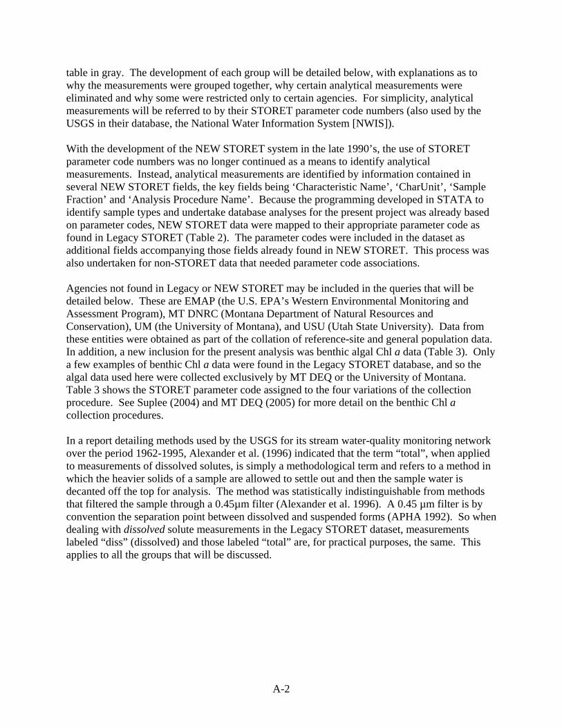
table in gray. The development of each group will be detailed below, with explanations as to why the measurements were grouped together, why certain analytical measurements were eliminated and why some were restricted only to certain agencies. For simplicity, analytical measurements will be referred to by their STORET parameter code numbers (also used by the USGS in their database, the National Water Information System [NWIS]). With the development of the NEW STORET system in the late 1990’s, the use of STORET parameter code numbers was no longer continued as a means to identify analytical measurements. Instead, analytical measurements are identified by information contained in several NEW STORET fields, the key fields being ‘Characteristic Name’, ‘CharUnit’, ‘Sample Fraction’ and ‘Analysis Procedure Name’. Because the programming developed in STATA to identify sample types and undertake database analyses for the present project was already based on parameter codes, NEW STORET data were mapped to their appropriate parameter code as found in Legacy STORET (Table 2). The parameter codes were included in the dataset as additional fields accompanying those fields already found in NEW STORET. This process was also undertaken for non-STORET data that needed parameter code associations. Agencies not found in Legacy or NEW STORET may be included in the queries that will be detailed below. These are EMAP (the U.S. EPA’s Western Environmental Monitoring and Assessment Program), MT DNRC (Montana Department of Natural Resources and Conservation), UM (the University of Montana), and USU (Utah State University). Data from these entities were obtained as part of the collation of reference-site and general population data. In addition, a new inclusion for the present analysis was benthic algal Chl a data (Table 3). Only a few examples of benthic Chl a data were found in the Legacy STORET database, and so the algal data used here were collected exclusively by MT DEQ or the University of Montana. Table 3 shows the STORET parameter code assigned to the four variations of the collection procedure. See Suplee (2004) and MT DEQ (2005) for more detail on the benthic Chl a collection procedures. In a report detailing methods used by the USGS for its stream water-quality monitoring network over the period 1962-1995, Alexander et al. (1996) indicated that the term “total”, when applied to measurements of dissolved solutes, is simply a methodological term and refers to a method in which the heavier solids of a sample are allowed to settle out and then the sample water is decanted off the top for analysis. The method was statistically indistinguishable from methods that filtered the sample through a 0.45µm filter (Alexander et al. 1996). A 0.45 µm filter is by convention the separation point between dissolved and suspended forms (APHA 1992). So when dealing with dissolved solute measurements in the Legacy STORET dataset, measurements labeled “diss” (dissolved) and those labeled “total” are, for practical purposes, the same. This applies to all the groups that will be discussed.
A-2
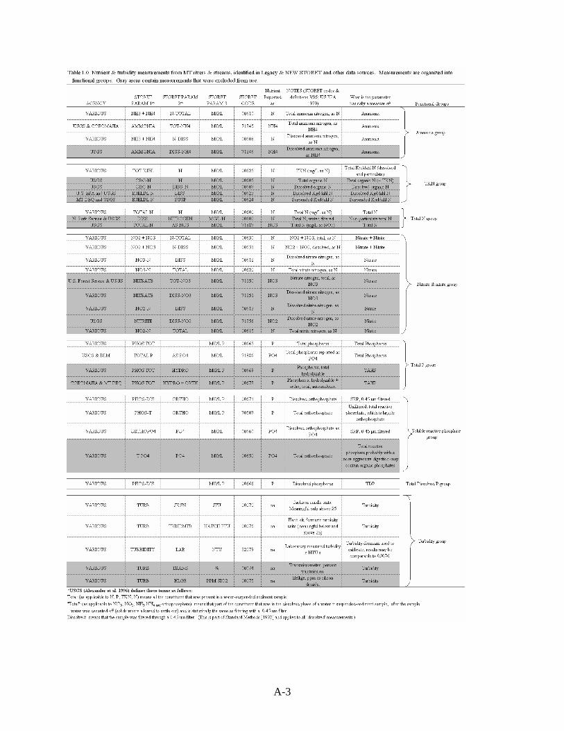
A-3

A-4
Table 3.0 Benthic chlorophyll a measurements from MT rivers & streams.
AGENCYSTORET
PARAM 1STORET PARAM
2STORET
PARAM 3STORET CODE* Values Reported as: NOTES
What is the parameter basically a measure of:
MT-DEQ and UM CHLRPHYL A MG/M2 CORRECTD 32223 mg Chl a /m2 Recorded as Rock in "Medium" field of NEW STORET.
Algal chlorophyll a from the surface of stream-bottom
rocks, collected with a template; values NOT
estimated.
MT-DEQ and UM CHLRPHYL A MG/M2 CORRECTD 32223 mg Chl a /m2 Recorded as Rock or Other in "Medium" field in NEW STORET.
Algal chlorophyll a from the surface of stream-bottom
rocks, six-rocks composited; values estimated (J).
MT-DEQ and UM CHLRPHYL A MG/M2 CORRECTD 32223 mg Chl a /m2 Recorded as Other in "Medium" field in NEW STORET.
Algal chlorophyll a collected using the Hoop Method.
MT-DEQ and UM CHLRPHYL A MG/M2 CORRECTD 32223 mg Chl a /m2 Recorded as Sediment in "Medium" field in NEW STORET.
Algal chlorophyll a collected using the Core Method.
* Although none of these data are from Legacy STORET, the parameter code and parameter names assigned are the equivelant values as found in Legacy STORET.

A. Ammonia Group The group was composed of four analytical measurements, all which measure ammonia and/or ammonium; 00610, 00608, 71845 and 71846 (Table 1.0). Only the USGS used 71846 and this parameter was eliminated, as it is similar to 71845 and the USGS frequently reported both 71845 and 71846 from the same sample. The USGS also frequently reported 00610, 00608, and 71845 from a single sample; so only one (00610) was retained to avoid same-sample duplication. All other agencies used 00610, 00608, and 71845, but did not report them from the same sample; so all values from those agencies could be retained. 71845 is reported as NH4 and, in order that the data be compatible with 00608 and 00610, all sample results for 71845 need to be multiplied by 0.7765 to convert them to ‘as N’. The database query has two important fields that are required to be correctly queried to produce the Ammonia Group: ‘Agency Code’ and ‘Param Code’. The query for the Ammonia Group should be written as follows: AGENCY CODE PARAM CODE Not “112WRD” 71845 Not “112WRD” 00608 00610 (Microsoft Access queries described in the remainder of this report will follow the general pattern shown above, and are applicable to the database which combines the ‘tblLEGSTORETGRAB(mostly nutrient)’ data and data from NEW STORET, EMAP and the Universities.) B. TKN /Organic N Group The database contained five analytical measurements in this group (00625, 00605, 00607, 00623, and 00624). The USGS reported from individual samples both 00625 (total Kjeldahl N) and 00605 (total organic N), and since 00605 is unique to the USGS it was eliminated. Many other different agencies reported 00625. 00607 (dissolved organic N) is unique to the USGS but is not useful in this effort because it excludes particulate organic N. Similarly, 00623 and 00624 measure either dissolved or suspended TKN, respectively, and therefore they were eliminated. The query was written to capture only 00625 and is shown here: AGENCY CODE PARAM CODE 00625 C. Total N Group Three TN analytical measurements were located in the database (00600, 00602 and 71887). 71887 is unique to the USGS and is frequently reported along with 00600 from the same samples (71887 is total N reported at NO3), and was eliminated from use. 00602 only measured total N
A-5

from the dissolved fraction and therefore is not comparable to 00600. The query for total N is as follows: AGENCY CODE PARAM CODE 00600 D. Nitrate + Nitrite Group This group contained the largest number of analytical measurement variations and presented the most complicated query challenge. At first, the possibility of summing the individual nitrate value and individual nitrite value (e.g., 71851 and 71856) from the same sample was considered, but this presented a major database effort in order to correctly match stations, dates and times for numerous different agencies. In most natural water exposed to oxygen, nitrite is only present in trace quantities and most dissolved inorganic N is nitrate (Horne and Goldman 1994). A review of this database showed that most nitrite measurements were very low or below the detection limit. Further, analytical measurements that analyzed for both NO3 + NO2 simultaneously (both 00630 and 00631 do this) were the largest contributors to the group in terms of sample numbers, and therefore nitrite is included in the bulk of the samples. For simplicity, it was decided to eliminate all nitrite-only measurements (00615, 00613, and 71856) from use (Table 1.0). Large numbers of USGS samples reported both 71851 (nitrate as NO3) and 00618 (nitrate dissolved, as N) from the same sample. But there were only 114 non-USGS records for 71851 (for streams & rivers) in the database. Therefore, 71851 was completely eliminated (Table 1.0). The USGS and the U.S. Forest Service were the only agencies to measure 71850 (“total” nitrate as NO3), and sometimes reported both 00618 and 71850 from the same samples; therefore, 71850 (the measurement with fewest values) was eliminated. The remaining four ‘nitrate’ or ‘nitrate + nitrite’ measurements (00630, 00631, 00618 and 00620) were queried on an agency-by-agency basis to determine which agencies reported more than one of these measurements from a single sample. It resulted that the USGS frequently reported all four, and so their samples are restricted in the query only to 00630 (NO3 + NO2 N-TOTAL). MT DEQ (agency code 21MTHDWQ) did, on very rare occasions, report 00630 and 00620 from the same sample, but in the vast majority of cases reported values were unique and so all four measurements are retained. EPA (agency code 11EPALES) usually reported 00630 paired with 00620, and so 00620 was excluded. EMAP reported both 00618 and 00631, but there were only a few 00631 samples so that parameter was eliminated for EMAP and 00618 was retained. None of the remaining agencies reported more than one of the four measurements from any single sample. 11NPSWRD was excluded because the few sample shown in the database appeared to be end-of-pipe data. The final query is shown below:
Agency Code Param CodeNot "112WRD" and Not "11NPSWRD" and Not "EMAP" 00631Not "11NPSWRD" 00630Not "112WRD" and Not "11NPSWRD" 00618Not "112WRD" and Not "11EPALES" and Not "11NPSWRD" 00620
A-6

E. Total P Group Comprised of four measurements (00665, 71886, 00669, and 00678). 00669 and 00678 were completely excluded because there was some uncertainty in the comparability of these samples to 00665 and 71886 and together, they represented < 1% of the data of this group. The two remaining measurements (00665 and 71886) were both found to be frequently reported on from a single sample by the USGS, and so the query restricts USGS data to 00665. All other agencies reported one or the other from any given sample. Values from 71886 are reported as PO4 and will need to be converted to units of P to combine with 00665, therefore all samples under the 71886 code need to be multiplied by 0.3261. The query is shown below: F. Soluble Reactive Phosphate (SRP) Group This group consists of four analytical measurements (00671, 70507, 00660, and 00650). 00650 was eliminated completely because of uncertainty in the comparability of this analytical measurement to the other three. The USGS frequently reported the remaining three (00671, 70507, 00660) from a single sample, but one of them (00660) was simply a reporting unit change (00660 is reported as PO4) and of the remaining two, there were six times more records for 00671 than for 70507. Therefore, for the USGS only 00671 is retained. EPA (agency code 1119C050) often reported 70507 and 00671 from a single sample and therefore the query restricts that agency to just 70507. The other agencies did not report more than one measurement from a single sample. The query is shown below: AGENCY CODE PARAM CODE Not “112WRD” 70507 Not “112WRD” 00660 Not “1119C050” 00671 G. Total Dissolved Phosphorus (TDP) Group Only one analytical measurement was found in the database (00666). No restrictions are placed on any agency for this query, which is shown below: AGENCY CODE PARAM CODE 00666 H. Turbidity Group Consists of five analytical turbidity measurements (00070, 00076, 82079, 00074, and 00075). 00075 was eliminated as no record of what it actually measures could be found. 00074 was eliminated after a conversation with the USGS revealed that 00074’s units (percent light light transmissivity) could not be directly converted to the other commonly used turbidity unit, JTU or NTU (John Lambing, personal communication). The remaining three measurements (00070, 00076, and 82079) are based on differing measurement methodologies relying on visible light and infrared light respectively. There is no consistent conversion mechanism that can be applied to standardize 00070 and 00076 measurements; the measurements (JTU and FTU) were therefore
A-7
analyzed separately. Further, 00070 (JTU) values are only meaningful when they are higher than 25 (Hach Chemical Co. 1975). 00076 (FTU) and 82079 (NTU) values are evidently comparable because 82079 values were calibrated using formazin; 00076 values are meaningful down to a value of 1.0 (Hach Chemical Co. 1975; APHA 1992), whereas 82079 values are meaningful down to 0.02 (APHA 1992). No agency reported all three, or pairs, from the same sample. After the query is run, all values associated with 00070 that are less than 25 should be eliminated, and in any analyses the values from 00070 should be kept separate from those of 00076 and 82079. The query is shown below:
Benthic Chlorophyll a Group
here is a single analytical measurement for this group (32223), although there are variations in
herein 6 stream-bottom rocks are collected and
f
eferences
lexander, R. B., Ludtke, A. S., Fitzgerald, K. K., and T. L. Schertz. 1996. Data from selected
merican Public Health Association (APHA). 1992. Standards methods for the examination of
ach Chemical Co. 1975. Procedures, chemical lists and glassware for water and wastewater
a.
orne, A. J., and C. R. Goldman. 1994. Limnology, 2 edition. McGraw-Hill.
AGENCY CODE PARAM CODE
Agency Code Param Code000700007682079
I. Tthe way benthic Chl a have been collected (Table 3; see Suplee 2004 or MT DEQ SOPs for moreexplanation). All of the samples have been adjusted for phaeophytins (monochromatic method; APHA 1992), and are only measures of algal Chl a. By definition one of the rock methods, wthe total attached Chl a is extracted (see Notes, table 3.0), is considered an estimate (“J” flag in the Remark_Code field). This is because it is assumed that the Chl a was recovered from 50% othe rocks’ total surface area, which may or may not be true. The query for these data is shown below. It should be noted that for this group in the present study, an exception is made to the general exclusion of estimated data (“J” flagged); this exception will apply only to datawith STORET parameter code 3223.
32223
R A
U.S. geological survey national stream water-quality monitoring networks (WQN) on CD-ROM. United States Geological Survey, Open-File Report 96-337.
Awater and wastewater, 18th edition. American Public Health Association, Washington, D.C.
Hanalysis with calibrations for the Bausch and Lomb Spectronic 20, Mini Spec 20 and other popular spectrophotometers. 2nd edition. Hach Chemical Company, Ames, Iow
ndH
A-8

Lambing, J. 2004. USGS Water Quality Specialist. Personal communication. Helena, MT,
T DEQ. 2005. Sample collection and laboratory analysis of chlorophyll-a, standard operation
TORET. 1996. Printout of STORET parameter numbers and their associated descriptions.
uplee, M. 2004. Wadeable streams of Montana’s Hi-line region: an analysis of their nature and
r_Doc_DII.pdf
May 10th, 2004.
Mprocedure. QPBWQM-011, review draft of 5/16/2005. Available from the MT Department of Environmental Quality, 1520 E. 6th Ave, Helena, MT 59620.
SPrinted from the EPA STORET system on September 11, 1996 (on file at the MT Department of Environmental Quality, Helena, MT).
Scondition, with an emphasis on factors affecting aquatic plant communities and recommendations to prevent nuisance algae conditions. Montana Department ofEnvironmental Quality, May 2004. Available at: http://www.deq.state.mt.us/wqinfo/Standards/Maste
U.S EPA. 1979. Methods for chemical analysis of water and wastes. United Stated 1979.
arghese, A. and J. Cleland. 2004a. Stratification of algae and nutrient data of Montana rivers
arghese, A. and J. Cleland. 2004b. Montana rivers and streams reference-to-whole-population
Environmental Protection Agency, publication No. EPA-600/4-79-020. March
Vand streams to assist in the development of numeric standards-final report. Submitted to Dr. Michael Suplee, Montana Department of Environmental Quality, Helena, MT. July 13, 2004.
Vpercentile mapping for selected water quality parameters-final report. Submitted to Dr. Michael Suplee, Montana Department of Environmental Quality, Helena, MT. November 19, 2004.
A-9

APPENDIX B
SEASONAL GROUPING METHODOLOGY
Prepared by: Dr. Michael Suplee, MT DEQ June 17, 2005
Techniques used to Determine Seasonal Periods for the Purpose of Segregating Nutrient
and Chlorophyll a Data by Time of Year The results of two previous analyses (Varghese and Cleland 2004; Varghese and Cleland 2005) demonstrated that level III and level IV ecoregions (Omernick 1987) are likely to be meaningful tools for the purpose of stratifying nutrient data in Montana. It was hypothesized that the correlation between ecoregions and nutrient concentrations might be further improved by dividing the data into different seasons, as nutrient concentrations in flowing waters often demonstrate distinct seasonal patterns (Lohman and Priscu 1992). For example, phosphorus (P) is frequently associated with total suspended sediment (TSS) and during spring runoff in streams both TSS and total P can be orders-of-magnitude higher than at other times (Horne and Goldman 1994). Seasonal variation in stream nutrient concentrations are not only influenced by abiotic factors such as runoff patterns, they are also influenced by biological uptake and release by organisms such as aquatic plants. Aquatic plant growth — including algal growth — is influenced by (among other things) light availability and temperature, which are climatically driven. Therefore, the development of seasons to define nutrient concentrations must consider not only hydrologic patterns, but climatic factors such as the onset of cold winter temperatures as well. The following describes techniques that were used to establish distinct seasonal periods, applicable to each of Montana’s seven level III ecoregions. The goal of this effort was to define three seasons for each ecoregion: a growing season, which would roughly correspond to the summer months; winter, which would follow the growing season; and runoff, which would terminate the winter period and comprise the yearly high flow period. 1. Selection of best-fit cutoff dates for the runoff period using hydrologic data. To address the hydrologic component, the United State Geological Survey (USGS) was consulted. The USGS indicated that flow-duration hydrographs for average daily flows could be a useful approach for describing typical, long-term flow conditions on any given stream (C. Parrett, personal communication). The data used in the present work were all extracted from the USGS’s online NWIS database. The flow duration hydrographs were developed using the complete period of record for USGS gauge stations in Montana that typically had a minimum of 10 years of continuous data. For each station, the average of all daily flow records for any given date was calculated. Each day of the year was plotted, and the hydrograph curve thus generated represents the average flow conditions at the station over the course of the year for the time period over which the data were collected (Fig. 1.0).
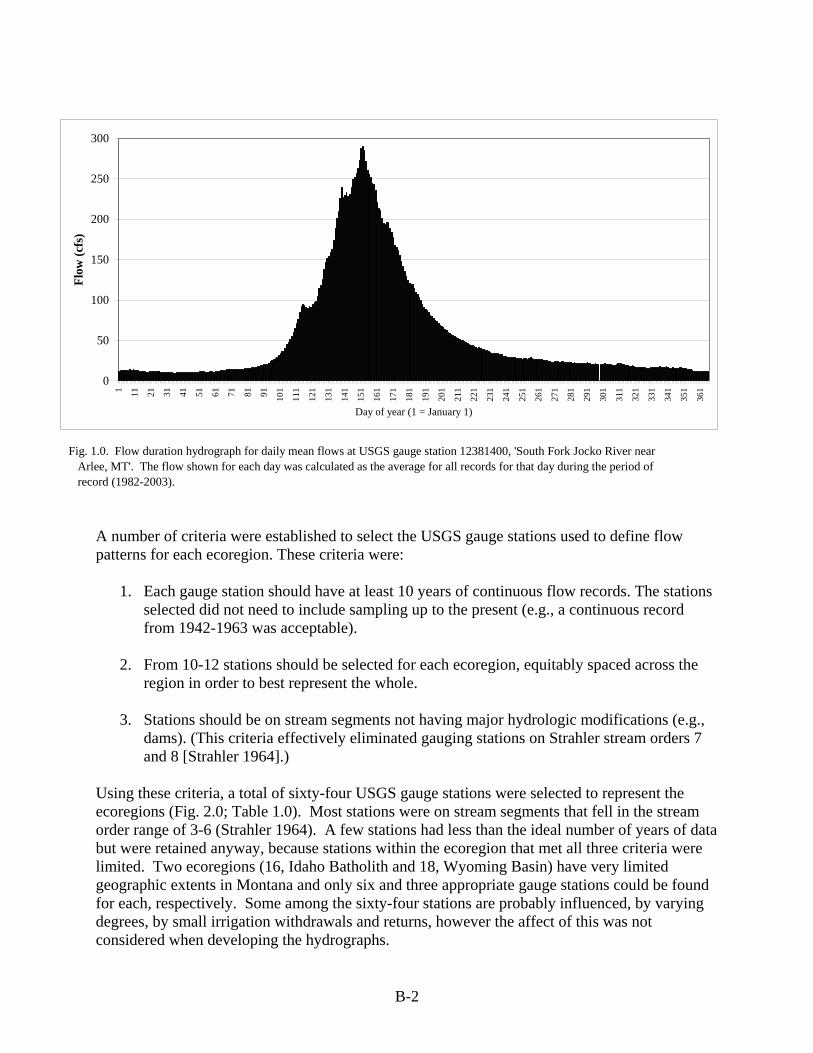
number of criteria were established to select the USGS gauge stations used to define flow
1. Each gauge station should have at least 10 years of continuous flow records. The stations
. From 10-12 stations should be selected for each ecoregion, equitably spaced across the
. Stations should be on stream segments not having major hydrologic modifications (e.g.,
sing these criteria, a total of sixty-four USGS gauge stations were selected to represent the
ta
ound
considered when developing the hydrographs.
Fig. 1.0. Flow duration hydrograph for daily mean flows at USGS gauge station 12381400, 'South Fork Jocko River near Arlee, MT'. The flow shown for each day was calculated as the average for all records for that day during the period of record (1982-2003).
0
50
100
150
200
250
300
1 11 21 31 41 51 61 71 81 91 101
111
121
131
141
151
161
171
181
191
201
211
221
231
241
251
261
271
281
291
301
311
321
331
341
351
361
Day of year (1 = January 1)
Flow
(cfs
)
Apatterns for each ecoregion. These criteria were:
selected did not need to include sampling up to the present (e.g., a continuous record from 1942-1963 was acceptable).
2region in order to best represent the whole.
3dams). (This criteria effectively eliminated gauging stations on Strahler stream orders 7 and 8 [Strahler 1964].)
Uecoregions (Fig. 2.0; Table 1.0). Most stations were on stream segments that fell in the streamorder range of 3-6 (Strahler 1964). A few stations had less than the ideal number of years of dabut were retained anyway, because stations within the ecoregion that met all three criteria were limited. Two ecoregions (16, Idaho Batholith and 18, Wyoming Basin) have very limited geographic extents in Montana and only six and three appropriate gauge stations could be ffor each, respectively. Some among the sixty-four stations are probably influenced, by varying degrees, by small irrigation withdrawals and returns, however the affect of this was not
B-2

Figure 2.0. Location of USGS gauging stations used to develop ecoregionally-based time periods. The seven Level III ecoregions are shown in color.
B-3

B-4

B-5
B-5

B-6
B-6
median ents of
stream rs at 3 times the m ny aquatic life
curve were used to
calcu . The two
ean- or me
distant s appeared to drive
d. In these scenarios, th 2. ing
was immnce has
from nutrient
21st
The selec
irly uniform well into Novemb reduced temp ination in the
nutrients
Two types of flow duration hydrograph were developed for each station; one based on daily ean flows, and one based on daily median flows. Median flow-duration hydrographs were
developed in the present work because studies in New Zealand show that 3 times the mannual flow is a useful flow variable which explains much of the variance in measurem
aquatic communities (Clausen and Biggs 1997). This is because scouring occuedian yearly flow, and scouring is a physical stressor that controls ma
populations (Clausen and Biggs 1997).
Specific onset and termination dates for the runoff period were identified on flow-duration hydrographs for both daily mean flows and daily median flows. For the flow-duration hydrographs based on daily means, the points of greatest inflection on the define the runoff onset and termination dates (e.g., day 101 and 205 in Fig. 1.0). For the flow-duration hydrographs based on daily medians, the median flow for any given station was first
lated using all records in the dataset, and then this values was multiplied by threedates straddling the runoff period that had flows equal to 3 times the median flow were then noted for that hydrograph.
The best overall results were achieved using the mean-based flow duration hydrographs. New Zealand is a mountainous country, and in the mountainous ecoregions (e.g. 15, Northern Rockies) there was generally good agreement in the dates selected using either the m
dian-based hydrographs. However, in the plains ecoregions this was not the case. The plains ecoregions (42, 43 and 18) frequently show bimodal runoff periods with an initial rise in flow in March followed by a lull and then, usually in June, a second surge as runoff frommountain influences occurs. In a few of the plains hydrographs, thunderstormmuch of the high flows and these were often scattered across the entire summer perio
e three-times-the-median-flow approach proved to be unworkable.
Selection of best-fit cutoff dates for the start of winter and the start of the growseason, based on biological considerations.
After the hydrologically-based dates for the onset and termination of runoff were compiled, it ediately obvious that the runoff termination dates suggested by many of the flow-
duration hydrographs were frequently extending deeper into the summer than experieshown there to be discernable scouring effects on aquatic life. As stated earlier, scouring flows
runoff influence aquatic life (Clausen and Biggs 1997) as well as nutrient concentrations (Snelder et al. 2004), but after this affect subsides biological influences on streamconcentrations are likely to become significant (Lohman and Priscu 1992). MT DEQ uses June
as the general start date for its biological sampling index period, as experience has shown that runoff effects (i.e., scouring) have usually subsided by that time.
tion of the start-of-winter date could not be determined using hydrograph characteristics. After runoff, a period of base flow begins which is often fa
er or December (Fig. 1.0). However, climatic influences in Montana (mainlyeratures and light intensity) typically cause, by the end of September, a term
growth of aquatic plant life. Once the aquatic plant life has begun to senesce uptake ofis reduced and decomposition begins to outweigh production. In general, the MT DEQ uses

September 21st as the termination date for the biological sampling index period, which is supported by work that has been undertaken on macroinvertebrates in Montana streams (Richards 1996). 3. Final selection of best-fit cutoff dates for the winter, run-off and growing season
periods. The final cutoff dates for the three seasons in each ecoregion are shown in Table 2.0. They were
For f runoff
re re, at least, on the declining leg of the runoff curve. The start of
inter was uniformly selected as October 1st, the closest date to the end of the DEQ’s indexing
raw-Hill Inc.
Table 2.0
Ecowing
er 30 1 September 30
eptember 30ptember 30
Northwestern March 15 June 15 June 16 September 30Northw ber 30
mber 30
derived using a combination of the methods and considerations discussed in 1 and 2 above. simplicity, all dates were rounded to the nearest mid- or end-of-month date. The start owas calculated as the average onset date of runoff for the set of daily mean flow-duration hydrographs for each ecoregion. The growing season cutoff dates were developed by considering both the hydrograph end-of-runoff dates and the biological index period dates. In ecoregions where more than half of the hydrographs still showed sizable flows on June 21st, the start of the growing season was extended to July 16th. By July 16th all of the hydrographs weapproaching base flow or wewperiod and a date by which most aquatic plant growth should be ended for the year.
. Best-fit cutoff dates, by level III ecoregion, for each of three seasons (winter, runoff and growing season).
oregion Name
Ecoregion Level III Number
Start of Winter
End of Winter
Start of Runoff
End of Runoff
Start of Growing Season
End of GrSeason
Canadian Rockies 41 October 1 April 14 April 15 June 30 July 1 SeptembNorthern Rockies 15 October 1 March 31 April 1 June 30 July
References Clausen, B., and B. J. F. Biggs. 1997. Relationships between benthic biota and hydrological
indices in New Zealand streams. Freshwater Biol. 38: 327-342. Horne, A. J., and C. R. Goldman. 1994. Limnology, 2nd edition. McG
estern Great Plains 43 October 1 February 29 March 1 June 30 July 1 SeptemWyoming Basin 18 October 1 April 14 April 15 June 30 July 1 Septe
Idaho Batholith 16 October 1 April 14 April 15 July 15 July 16 SMiddle Rockies 17 October 1 April 14 April 15 July 15 July 16 SeGlaciated Plains 42 October 1 March 14
Lohman, K., and J. C. Priscu. 1992. Physiological indicators of nutrient deficiency in
Cladophora (chlorophyta) in the Clark Fork of the Columbia River, Montana. J. Phycol. 28: 443-448.
Omernik, J. M. 1987. Ecoregions of the conterminous United States. Annals of the Association
of American Geographers 77: 118-125.
B-7

Parrett, C. Hydrologist, United State Geological Survey, Helena, MT. Personal commun
February 24ication.
, 2005.
ain streams. M.S. thesis, Montana State University, Bozeman, MT, pp 166.
works. In
n
November 19, 2004.
Richards, D.C. 1996. The use of aquatic macroinvertebrates as water quality indicators in
mount Snelder, T. H., Biggs, B. J. F., and M. A. Weatherhead. 2004. Nutrient concentration criteria
and characterization of patterns in trophic state for rivers in heterogeneous landscapes. Journal of the American Water Resources Association 40: 1-13.
Strahler, A. N. 1964. Quantitative geomorphology of drainage basins and channel net
Chow, V. T. (ed), Handbook of applied hydrology. McGraw-Hill, New York, pp 439-476.
Varghese, A. and J. Cleland. 2004. Montana rivers and streams reference-to-whole-populatio
percentile mapping for selected water quality parameters-final report. Submitted to Dr. Michael Suplee, Montana Department of Environmental Quality, Helena, MT.
Varghese, A. and J. Cleland. 2005. Stratification of nutrient data for Montana rivers and
streams-summary of findings. Submitted to Dr. Michael Suplee, Montana Department of Environmental Quality, Helena, MT. February 15, 2005.
B-8

APPENDIX C
LITHOGRAPHIC GROUPING METHODOLOGY
Nutrient – Lithology – Geology Layer June 7, 2004
Jim Stimson (DEQ Source Water Protection Program) Source of Geologic Information: Gary L. Raines and Bruce R. Johnson, 1996, Digital representation of the Montana state geologic map: a contribution to the Interior Columbia River Basin Ecosystem Management Project, USGS Open File Report 95-691, ArcView Shapefile for Montana. Source of information on geologic sources of Nitrogen: Holloway, J.M., Dahlgren, R.A., and Casey, W. H., 1998, Contribution of bedrock nitrogen to high nitrate concentrations in stream water, Nature: Vol 395 October 1998, p. 785 – 788. Reason for lithology groupings: Based on information from the Holloway et al. study forms of nitrate (ammonium) can substitute into the mica crystal structure. In addition, several other sources identify marine shale rocks as containing significant amounts of nitrate. Therefore, sedimentary shale rocks and metamorphic that contain significant volumes of mica minerals, like biotite and muscovite, were two of the lithology categories culled out of the digital version of the 1955 Geologic map of Montana. How the lithology groupings were made: The digital version of the 1955 Geologic map of Montana comes with an attribute data table that includes multiple fields including eight lithology fields. In transferring the original lithologic descriptions from the 1955 geologic map, the dominant lithology type was placed into the Lith1 field, the next abundant lithology was placed into the Lith2 field, and so on. These lithology fields were used to isolate 17 lithology types. The dominant lithology names taken from the Lith1 and Lith2 fields are included in the lithology shapefile names. A quick review of the attribute table of each shapefile shows which specific lithologies are included in each group. Once a group of lithology types was selected from the original geologic shapefile, the selected records were exported into a new shapefile bearing the name of new lithologic group. Lithologic Groups: The following lithologic shapefiles have been created:
1) Igneous Intrusives and extrusives but not volcanics. Major types of igneous rock. Volcanics excluded.
2) Igneous volcanics. Rocks identified specifically as volcanics.
3) Metamorphic Schist. Schist is a name applied a metamorphic rock dominated by
aligned mica minerals usually biotite and muscovite but there is a host of other mica

minerals. Because the schist rocks contain significant volumes of mica minerals they are thought to be a possible source of geologic nitrate.
4) Metamorphic Schist and Argillite. Argillite is a name usually applied a fine-grained
rock like a shale or mudstone that is quite hard and breaks into angular “chucks”. Argillites are thought to have been metamorphosed so that the original minerals have been re-crystallized and have grown, and exhibit alignment with the general bedding direction. Because the argillite rocks contain significant volumes of mica minerals they are thought to be a possible source of geologic nitrate.
5) Sedimentary Sandstones. Thought to not be a source of geologic nitrate.
6) Sedimentary Quartzite. A metamorphosed sandstone composed almost entirely of
quartz grains. Thought to not be a source of geologic nitrate. 7) Sedimentary Gravel, Boulders, and Conglomerates. Range front gravel deposits and
the Flaxville gravels. Flaxville gravels host aquifers that can have elevated nitrate levels related to agricultural practices. Otherwise, thought to not be a source of geologic nitrate.
8) Sedimentary Limestone and Dolomite. Thought to not be a source of geologic nitrate.
9) Sedimentary Argillaceous Limestone. Limestones with a significant volume of fine
grained material (argillite) and could be a source of geologic nitrate.
10) Sedimentary Shaly Sandstone. Sandstones with a significant volume of shale and could be a source of geologic nitrate.
11) Sedimentary Sandy Shale. Sandstones with a significant volume of shale and could be
a source of geologic nitrate.
12) Sedimentary Shale and Clay. A grouping of several geologic formations where the Lith1 and Lith2 fields listed shale and clay. Could be a source of geologic nitrate.
13) Sedimentary Carbonaceous Shale. Shales with high organic (carbonaceous) content.
Could be a source of geologic nitrate.
14) Sedimentary Siliceous Shale. Shales with relatively high silica content. Could be a source of geologic nitrate.
15) Sedimentary Calcareous Shale. Shales with relatively high carbonate (calcite or
dolomite, or other carbonates) content. Could be a source of geologic nitrate.
16) Sedimentary Argillaceous Shale. I believe these are shales with relatively high mica content. There could also be shales that are more lithified and hard but I think the term is used to express that the rock has identifiably large mica crystals present. Could be a source of geologic nitrate.
C-2

17) Sedimentary Silt Dominated. Since there can be a fine line between shales and silts, I
pulled out formations that listed silt as the dominant lithology. Usually the term silt is used to describe rocks that are more gritty than shales or clays because the silt rock contains more grains of quartz. If they are associated with shale beds, they could be a source of geologic nitrate.
18) Sedimentary Silt Shale – Hell Creek Formation. The Hell Creek is part of the Fort
Union Formation and is usually described as containing more shale beds than the Fox Hills member (located below the Hell Creek) and the Tongue River member (located above the Hell Creek. Could be a source of geologic nitrate.
C-3

APPENDIX D
LOG FILES OF STATA STATISTICAL ANALYSES
Enclosed with this report is a CD-ROM that contains the detailed output of the statistical analyses conducted for this project. The CD contains several hundred statistical analyses (i.e., Stata log files) for ten water quality parameters evaluated in various combinations of coarse- and fine-scale stratifying parameters, as described in Section 4 of the report. Some analyses were repeated with both databases utilized for this project: the All-Observations database and the Median database. Below, we provide guidance on locating the files on the CD and finding specific statistical results within the log files. 1.1 Contents of Folders
The RUNS folder on the CD-ROM contains six folders. Table D-1 describes the contents of each folder and the databases analyzed. Table D-1: Folder Contents Folder Name Contents Databases Analyzed PTILE
Percentile Mapping
All-Observation Database
TESTS Significance Testing of Stratification Methods
Median Database
MCV Measures of Variation for Stratification Methods
All-Observation and Median Database
SEASONS Testing of Seasonal Differences
All-Observation and Median Database
STRAHDIST Distribution of Strahler Stream OrderIn General and Reference Population
All-Observation and Median Database
NO7&8 Repeats the analyses of the PTILE, TESTS and MCV folders for the general population after excluding Strahler stream order 7 and 8.
All-Observation and Median Database
Detailed guides to the contents of each folder are provided in Section 2 of this appendix.

1.2 Summary Statistics
Summary statistics of the water quality parameters are found in numerous places in the log files. Table D-2 describes where specific summary statistics may be located. Table D-2: Location of Summary Statistics Database Location of Summary Statistics Comment
All-Observation Folder = PTILE.
Locate log-file within sub-folder for specific nutrient and stratifying methodology of interest (coarse or fine).
Summary Statistics are presented for each level of various coarse/fine stratification methodologies for each season. General population and reference statistics are presented together.
Median Folder = TESTS Locate log-file within sub-folder for specific nutrient and stratifying methodology of interest (coarse or fine). Separate log-files are provided for general population and reference population results.
Summary Statistics are presented for each level of various coarse/fine stratification methodologies for each season. General population and reference statistics are NOT presented together but in separate log files.
1.3 Guide to Terminology
The log files contain a number of symbols, or codes, used as short-hand for water quality parameters and stratifying parameters in the database and in the statistical programs. In many cases, the log files provide comments that translate these symbols or codes into plain English equivalents. However, such translation was not always possible, given the complexity of some of the procedures. Therefore, the tables below provide a key to the codes used in this analysis.
Tables D-3, D-4 and D-5 list the codes used for water quality parameters, stratifying parameters, and geologic formations, respectively. Figure D-1 presents the codes used to represent Omernik Levels III and IV ecoregions.
D-2

Table D-3: Water Quality Parameter Codes
Code Water Quality Parameter AMMONIA Ammonia (mg/l) BNCHLOR-A Benthic Chlorophyll-a (mg/m2) NO3+NO2 Nitrate and Nitrite group (mg/l) SRP Soluble Reactive Phosphate (mg/l) TDP Total Dissolved Phosphorus (mg/l) TKN Total Kjeldahl Nitrogen (mg/l) TOTALN Total Nitrogen (mg/l) TOTALP Total Phosphorus (mg/l) TURB-NTU Turbidity (NTU) TURB-JTU Turbidity (JTU)
Table D-4: Stratifying Parameter Codes
Code Stratifying Parameter eco3 Omernik level III ecoregions eco4 Omernik level IV ecoregions sfname Geologic formation geco Grouped level III ecoregions (Mountain or Prairie) strahgroup Grouped Strahler Stream Order (1&2, 3&4, 5&6 and 7&8)
Table D-5: Geologic Formation Codes
Code Geologic Formation 1 Metamorphic Argillite 2 Argillaceous Shale 3 Argillaceous Limestone 4 Calcareous Shale 5 Carbonaceous Shale 6 Gravel, Boulders, Conglomerate 7 Hell Creek Silty Shale 8 Chert 9 Igneous but not Volcanic 10 Limestone and Dolomite 11 Quartzite 12 Sedimentary Sandstone 13 Sandy Shale 14 Metamorphic Schist 15 Shale and Clay 16 Shaly Sandstone 17 Siliceous Shale 18 Sedimentary Silt Dominated 19 Cretaceous and Tertiary Volcanics
D-3

USDA Natural ResourcesConservation Service
Albers equal area projectionStandard parallels 46° N and 48° N
15 10 5 0 30 60
030 20 10 60 120 km
mi
15 Northern Rockies15a Grave Creek Range-Nine Mile Divide15b Camas Valley15c Flathead Valley15d Tobacco Plains15e Flathead Hills and Mountains15h High Northern Rockies15i Clearwater Mountains and Breaks15k Clark Fork Valley and Mountains15l Salish Mountains15o Coeur d' Alene Metasedimentary Zone15p St. Joe Schist-Gneiss Zone15q Purcell-Cabinet-North Bitterroot Mountains15t Stillwater-Swan Wooded Valley
16 Idaho Batholith16a Eastern Batholith16b Lochsa Uplands16e Glaciated Bitterroot Mountains and Canyons16h High Idaho Batholith
17 Middle Rockies 17d Eastern Gravelly Mountains17e Barren Mountains17f Crazy Mountains17g Absaroka-Gallatin-Madison-Bridger
Sedimentary Mountains17h High Elevation Rockland Alpine Zone17i Absaroka-Gallatin Volcanic Mountains17j West Yellowstone Plateau17k Lady of the Lake17l Gneissic-Schistose Forested Mountains17m Big Horn-Pryor Mountains17p Foothill Potholes17q Big Snowy-Little Belt Carbonate Mountains17r Scattered Eastern Igneous-Core Mountains17s Bitterroot-Frenchtown Valley17t Limy Foothill Savanna17u Paradise Valley17v Big Belt Forested Highlands17w Townsend Basin17x Rattlesnake-Blackfoot-South Swan-Northern
Garnet-Sapphire Mountains17y Townsend-Horseshoe-London Sedimentary
Hills
17z Tobacco Root Mountains17aa Dry Intermontane Sagebrush Valleys17ab Dry Gneissic-Schistose-Volcanic Hills17ac Big Hole17ae Forested Beaverhead Mountains17af Centennial Basin17ag Pioneer-Anaconda Ranges17ah Eastern Pioneer Sedimentary Mountains17ai Elkhorn Mountains-Boulder Batholith17aj Eastern Divide Mountains17ak Deer Lodge-Philipsburg-Avon Grassy
Intermontane Hills and Valleys17al Southern Garnet Sedimentary-Volcanic
Mountains17am Flint Creek-Anaconda Mountains
18 Wyoming Basin18b Northern semiarid Intermontaine Basin
41 Canadian Rockies41a Northern Front41b Crestal Alpine-Subalpine Zone41c Western Canadian Rockies41d Southern Carbonate Front41e Flathead Thrust Faulted Carbonate-Rich
Mountains
42 Northwestern Glaciated Plains42b Collapsed Glacial Outwash42d Northern Missouri Coteau42i Glaciated Dark Brown Prairie42j Glaciated Northern Grasslands42k Coteau Lakes Upland42l Sweetgrass Uplands42m Cherry Patch Moraines42n Milk River Pothole Upland42o North Central Brown Glaciated Plains42q Rocky Mountain Front Foothill Potholes42r Foothill Grassland
43 Northwestern Great Plains 43a Missouri Plateau43b Little Missouri Badlands43c River Breaks43d Forested Buttes43e Sagebrush Steppe43g Semiarid Pierre Shale Plains43k Dense Clay Prairie43l Missouri Breaks Woodland-Scrubland43m Judith Basin Grassland43n Central Grassland43o Unglaciated Montana High Plains43p Ponderosa Pine Forest-Savanna Hills43q Mesic Tongue River Dissected Plains43s Non-calcareous foothill grassland43t Shield-Smith Valleys43u Limy Foothill Grassland43v Pryor-Big Horn Foothills
Level III ecoregionLevel IV ecoregionCounty boundaryState boundaryInternational boundary
15q15l
15t
15h15d
41c
41c
41b41a
41a
42q
42r
42n
42n
42o
42l42r
17r
15h
42r
42j
17r
42q
15c
15c
42m
42r
15k
15o
42i
41d
15o
42k42d
15l
41d
15e
15b
42b
41e
15e
42r
17r
42r
42d
15a
43n
15p
42i
43l
43l42q
43n
42r17r
41b
15a
17x
43c
15c
17s
43c
43c
42r
41b41b
41b
41b
41b 41b
43n
43n
17r
42q
15h
43m
43n43o
17r17p
17aj
43c
43u
43s
43a
17ak17x
17al16b
17q
17q
43s17r
43a
17x
17w
17w
17v
17al
43t
17t
17am
17aj
17ai
43u
43e
17ak
17q
16e
16a
17y
43o
43n
43s
43e
17f
17ag
43p
17ag
17ac
17g
17ah
17aa
17y
17ag
16h
16h
43c
43c
17h
17h
17h
17y
43p
17ab
43b
17l
43s
17y 17i
17ae
43p
43p
17ab
17ab
17z
43p
43p 43p
43p
17z
43c
17ab
17ab
43n
17g17g
43p
17l
17g17i
17u
17aa
17aa
17y
17l
43v
17e
17i17g
43p
17ad
43d
17e
17e
17d
43d
17e
43v
17l
17h
43d
17e17e
17e
17m
43n
18b
17ab
17ab
17h
17h
17k
17j
17m 43q
17j17af
43p
17e
43k
43g43g
15h
15h
15h
42r
17h
17h
17h
17h
17h
17h
Helena
Billings
Bozeman
Butte
Cut Bank
Great Falls
Havre
Kalispell
Miles City
Missoula
Wolf Point
Cody
Sheridan
Shelby
Baker
Broadus
Dillon
Livingston
Big Timber
Columbus
Red Lodge
Hardin
Forsyth
Roundup
White Sulphur Springs
Harlowton
Anaconda Boulder
Deer Lodge
TownsendHamilton
Superior
Lewistown
Jordan
Glendive
Sidney
Fort Benton
Choteau
PolsonThompsonFalls
Libby
Conrad
Chinook
Glasgow
Malta
PlentywoodScobey
Colstrip
Salmon
Fresno
MedicineLake
Reservoir
LakeElwell
Fla
thea
d La
ke
Lak
e K
ooca
nusa
CanyonFerry
Lake
HebgenLake
LakeYellowstone
F ort Pec
k Lak
e
Missouri River
Flathead River
Clark Fork
Flathead River
Miss
ouri River
Missouri R
iver
Missouri River
Musselshell R
iver
Yello
wst
one
Rive
r
Yellowstone River
Musselshell River
S
almon River
Bit
terr
oot R
iver
Clark Fork
Kooten
ai River
Milk River
Teton River
Marias River
Powde
r Ri
ver
Sage Creek
Big
San
dy C
reek
CANADA
UNITED STATES
ALBERTA SASKATCHEWAN
BRITISH COLUMBIA
IDA
HO
NO
RT
H D
AK
OTA
WYOMING
WY
OM
ING
IDA
HO
SOU
TH
DA
KO
TA
116° 115° 114° 113° 112° 111° 110° 109° 108° 107° 106° 105° 104°
115° 114° 113° 112° 111° 110° 109° 108° 107° 106°105°
45°
46°
47°
48°
49°
45°
46°
47°
48°
49°
IN T E R IOR —G E OLOG ICA L S U R V E Y , R E S T ON , V IR G IN IA —1999
Ecoregions of Montana

2. Detailed Guide to Folders 2.1 PTILE
The PTILE folder contains two separate sub-folders for coarse and fine-scale stratifications. Each of these contains ten sub-folders, one for each water quality parameter. Within the water quality parameter subfolder, are further subfolders for each stratification methodology.
For example, to access the percentile mapping results for TKN by Geologic Formation, follow the path:
Ptile/Coarse/TKN/SFNAME and open the log file TKN.log
To access the percentile mapping results for SRP by Omernik level III ecoregions by Geologic Formation, follow the path:
Ptile/Fine/SRP/ECO3/SFNAME and open the log file SRP.log.
The coarse-scale log files have the following general structure:
For each level of the coarse-scale stratifying variable, each season is considered in turn. For each season, the log file contains summary statistics, tests of comparison for the reference and general population, and the results of the percentile mapping. After all seasons have been considered, the analysis moves to the next level of the stratifying variable.
The fine-scale log files have the same structure, except that the analysis is performed for
each level of the fine-scale parameter within each level of the coarse-scale parameter.
Our previous report (ICF 2004b) provided an annotated guide to the percentile mapping log files, which are nearly identical to those in this analysis and may be consulted for further details on interpreting the log files.
The analyses are supported by a series of graphics, which display adjacent box-whisker plots for logtransformed data for the non-reference and reference populations. An example graph is displayed below. (In the graphs, “Y” refers to the reference population and “N” to the non-reference population.)
D-5
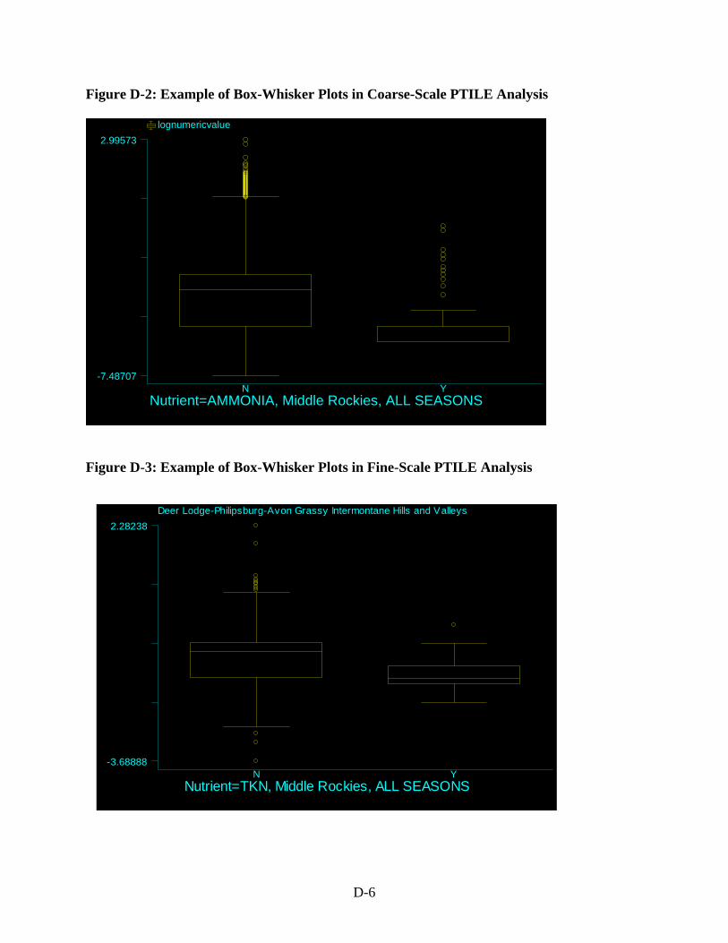
Figure D-2: Example of Box-Whisker Plots in Coarse-Scale PTILE Analysis
Nutrient=AMMONIA, Middle Rockies, ALL SEASONS
-7.48707
2.99573 lognumericvalue
N Y
Figure D-3: Example of Box-Whisker Plots in Fine-Scale PTILE Analysis
Deer Lodge-Philipsburg-Avon Grassy Intermontane Hills and Valleys
Nutrient=TKN, Middle Rockies, ALL SEASONS
-3.68888
2.28238
N Y
D-6

2.2 TESTS
The TESTS folder contains two separate sub-folders for coarse and fine-scale stratifications. Each of the sub-folders contains a sub-folder for General Population results (GP) and a sub-folder for Reference Population results (REF). Each of these contains ten sub-folders, one for each water quality parameter. Within the water quality parameter subfolders, are further subfolders for each stratification methodology.
For example, to access the significance testing results for TKN by Geologic Formation in the General Population, follow the path:
Tests/Coarse/GP/TKN/SFNAME and open the log file TKNsfnameGP.log
To access the percentile mapping results for SRP by Omernik level III ecoregions by Geologic Formation in the Reference Population, follow the path:
Tests/Fine/REF/SRP/ECO3/SFNAME and open the log file SRPeco3sfnameREF.log.
The coarse-scale log files have the following general structure:
A separate analysis is performed for each season. First, summary statistics are reported for each level of the stratifying parameter for the nutrient, for the specific season.
An example output of summary statistics is presented below: _________________________________________________________________ SUMMARY STATISTICS for Nutrient = TKN by Level 3 Ecoregion for Season = ALL SEASONS Summary for variables: num by categories of: eco3 eco3 | N min max mean sd skewness -----+------------------------------------------------------------ 15 | 342.00 0.03 23.70 0.42 1.50 13.09 16 | 39.00 0.05 2.00 0.39 0.45 1.63 17 | 764.00 0.03 69.30 0.48 2.55 25.75 18 | 10.00 0.17 2.89 0.73 0.81 2.11 41 | 43.00 0.05 1.00 0.22 0.23 1.53 42 | 259.00 0.05 13.00 1.02 1.35 4.93 43 | 645.00 0.03 51.40 0.87 2.23 18.50 -----+------------------------------------------------------------ Total| 2102.00 0.03 69.30 0.65 2.13 23.40 ------------------------------------------------------------------ Summary for variables: num by categories of: eco3 eco3 | N p10 p25 p50 p75 p90 -----+------------------------------------------------------------ 15 | 342.00 0.05 0.10 0.20 0.50 0.65 16 | 39.00 0.05 0.05 0.13 0.50 1.10 17 | 764.00 0.05 0.10 0.25 0.50 0.80 18 | 10.00 0.18 0.22 0.51 0.74 2.00 41 | 43.00 0.05 0.05 0.11 0.30 0.60 42 | 259.00 0.20 0.34 0.70 1.16 1.90 43 | 645.00 0.14 0.28 0.52 1.00 1.60 -----+------------------------------------------------------------ Total| 2102.00 0.05 0.15 0.35 0.70 1.26 ------------------------------------------------------------------ _________________________________________________________________
D-7

XXXXXXXXXXXXXXXXXXXXXXXXXXXXXXXXXXXXXXXXXXXXXXXXX
The Kruskal Wallis (KW) Test for equality of median nutrient concentrations across each stratum is then performed. An example output of the KW test is presented below: KRUSKAL-WALLIS TEST for Nutrient = TKN by Level 3 Ecoregion for Season = ALL SEASONS Test: Equality of populations (Kruskal-Wallis test) eco3 _Obs _RankSum 15 342 269425.00 16 39 32788.50 17 764 657985.00 18 10 12734.00 41 43 26377.00 42 259 370142.00 43 645 840801.50 chi-squared = 379.591 with 6 d.f. probability = 0.0001 chi-squared with ties = 380.900 with 6 d.f. probability = 0.0001 ______________________________________________________ Can Reject the Hypothesis that the group medians are equal ______________________________________________________
Note that the statistical results are interpreted by an explanatory comment. XXXXXXXXXXXXXXXXXXXXXXXXXXXXXXXXXXXXXXXXXXXXXXXXX
The KW test is followed by a non-parametric multiple comparison of means. An annotated abbreviated example output of the non-parametric multiple comparisons of means is presented below. (Note: the yellow-highlighted comments have been added here to facilitate interpretation and are not part of the log files.) NON-PARAMETRIC MULTIPLE COMPARISON OF MEDIANS One-way analysis of variance by ranks (Kruskal-Wallis Test) neco3 Obs RankSum RankMean -------------------------------- 1 342 269425.00 787.79 2 39 32788.50 840.73 3 764 657985.00 861.24 4 10 12734.00 1273.40 5 43 26377.00 613.42 6 259 370142.00 1429.12 7 645 840801.50 1303.57 Chi-squared (uncorrected for ties) = 379.591 with 6 d.f. (p = 0.00010) Chi-squared (corrected for ties) = 380.900 with 6 d.f. (p = 0.00010) Multiple comparisons between groups ----------------------------------- (Adjusted p-value for significance is 0.001190)
D-8

Ho: num(neco3==1) = num(neco3==2) RankMeans difference = 52.94 Critical value = 311.65 Prob = 0.302903 (NS) THE NULL HYPOTHESIS IS THAT THE MEDIAN VALUE FOR NECO3=1 IS EQUAL TO THE MEDIAN VALUE FOR NECO3=2. NECO3 IS THE CODENAME FOR ECO3. A RELATIONSHIP KEY AT THE END OF THE ANALYSIS WILL ASSOCIATE THE NUMERIC VALUES WITH SPECIFIC LEVELS OF THE STRATIFYING PARAMETER. THE OPERATIVE TERM TO INTERPRETING THE RESULTS HERE IS THE “NS” IN PARENTHESIS, WHICH STANDS FOR “NOT SIGNIFICANT”. THIS IMPLIES THAT THE DIFFERENCE BETWEEN THE MEDIANS OF THE TWO GROUPS COMPARED IS NOT SIGNIFICANT. Ho: num(neco3==2) = num(neco3==7) RankMeans difference = 462.84 Critical value = 304.06 Prob = 0.000002 (S)
THE NULL HYPOTHESIS IS THAT THE MEDIAN VALUE FOR NECO3=2 IS EQUAL TO THE MEDIAN VALUE FOR NECO3=7. BECAUSE THE TERM IN PARENTHESIS IS “S”, THIS IMPLIES THAT THE DIFFERENCE BETWEEN THE MEDIANS OF THE TWO GROUPS COMPARED IS INDEED SIGNIFICANT.
XXXXXXXXXXXXXXXXXXXXXXXXXXXXXXXXXXXXXXXXXXXXXXXXX
Here is the relationship key for the stratifying variable: RELATIONSHIP KEY FOR MULTIPLE COMPARISON TESTS ---------------------------------------------------- group(eco | eco3 3) | 15 16 17 18 41 42 43 ----------+----------------------------------------- 1 | 342 2 | 39 3 | 764 4 | 10 5 | 43 6 | 259 7 | 645 ----------------------------------------------------
According to this key, the numeric group 1 refers to the level III ecoregion with the
codename 15, which is the Northern Rockies (see figure D-1). XXXXXXXXXXXXXXXXXXXXXXXXXXXXXXXXXXXXXXXXXXXXXXXXX
The log file then presents the results of a one-way analysis of variance to test the statistical significance of the stratifying parameter. An example output of the ANOVA procedure is presented below: ANOVA for Nutrient = TKN by Level 3 Ecoregion for Season = ALL SEASONS Number of obs = 2102 R-squared = 0.1707 Root MSE = 1.04184 Adj R-squared = 0.1683 Source | Partial SS df MS F Prob > F -----------+---------------------------------------------------- Model | 468.139391 6 78.0232318 71.88 0.0000 | neco3 | 468.139391 6 78.0232318 71.88 0.0000 | Residual | 2273.99068 2095 1.08543708 -----------+---------------------------------------------------- Total | 2742.13007 2101 1.30515472
D-9
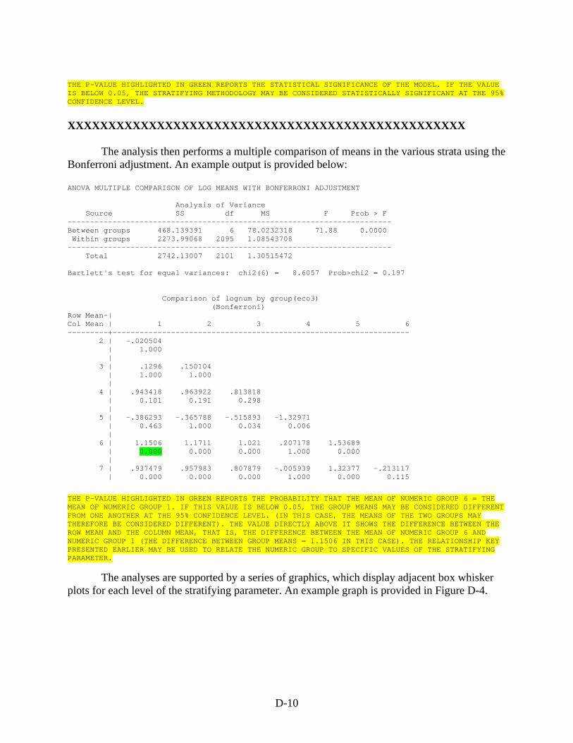
THE P-VALUE HIGHLIGHTED IN GREEN REPORTS THE STATISTICAL SIGNIFICANCE OF THE MODEL. IF THE VALUE IS BELOW 0.05, THE STRATIFYING METHODOLOGY MAY BE CONSIDERED STATISTICALLY SIGNIFICANT AT THE 95% CONFIDENCE LEVEL. XXXXXXXXXXXXXXXXXXXXXXXXXXXXXXXXXXXXXXXXXXXXXXXXX
The analysis then performs a multiple comparison of means in the various strata using the Bonferroni adjustment. An example output is provided below: ANOVA MULTIPLE COMPARISON OF LOG MEANS WITH BONFERRONI ADJUSTMENT Analysis of Variance Source SS df MS F Prob > F ------------------------------------------------------------------------ Between groups 468.139391 6 78.0232318 71.88 0.0000 Within groups 2273.99068 2095 1.08543708 ------------------------------------------------------------------------ Total 2742.13007 2101 1.30515472 Bartlett's test for equal variances: chi2(6) = 8.6057 Prob>chi2 = 0.197 Comparison of lognum by group(eco3) (Bonferroni) Row Mean-| Col Mean | 1 2 3 4 5 6 ---------+------------------------------------------------------------------ 2 | -.020504 | 1.000 | 3 | .1296 .150104 | 1.000 1.000 | 4 | .943418 .963922 .813818 | 0.101 0.191 0.298 | 5 | -.386293 -.365788 -.515893 -1.32971 | 0.463 1.000 0.034 0.006 | 6 | 1.1506 1.1711 1.021 .207178 1.53689 | 0.000 0.000 0.000 1.000 0.000 | 7 | .937479 .957983 .807879 -.005939 1.32377 -.213117 | 0.000 0.000 0.000 1.000 0.000 0.115
THE P-VALUE HIGHLIGHTED IN GREEN REPORTS THE PROBABILITY THAT THE MEAN OF NUMERIC GROUP 6 = THE MEAN OF NUMERIC GROUP 1. IF THIS VALUE IS BELOW 0.05, THE GROUP MEANS MAY BE CONSIDERED DIFFERENT FROM ONE ANOTHER AT THE 95% CONFIDENCE LEVEL. (IN THIS CASE, THE MEANS OF THE TWO GROUPS MAY THEREFORE BE CONSIDERED DIFFERENT). THE VALUE DIRECTLY ABOVE IT SHOWS THE DIFFERENCE BETWEEN THE ROW MEAN AND THE COLUMN MEAN, THAT IS, THE DIFFERENCE BETWEEN THE MEAN OF NUMERIC GROUP 6 AND NUMERIC GROUP 1 (THE DIFFERENCE BETWEEN GROUP MEANS = 1.1506 IN THIS CASE). THE RELATIONSHIP KEY PRESENTED EARLIER MAY BE USED TO RELATE THE NUMERIC GROUP TO SPECIFIC VALUES OF THE STRATIFYING PARAMETER.
The analyses are supported by a series of graphics, which display adjacent box whisker plots for each level of the stratifying parameter. An example graph is provided in Figure D-4.
D-10

Figure D-4: Example of Box-Whisker Plots in Coarse-Scale TESTS Analysis
Grouped By Level 3 Ecoregion
Nutrient=TKN, Season= ALL SEASONS
-4.14703
4.23844
15 16 17 18 41 42 43
XXXXXXXXXXXXXXXXXXXXXXXXXXXXXXXXXXXXXXXXXXXXXXXXX
The fine-scale analyses for the significance of sub-stratifying methodologies have a different structure than the coarse-scale.
These analyses first report exploratory one-way ANOVA on the coarse-scale parameter, one-way ANOVA on the fine-scale parameter, two-way factorial ANOVA with interaction on the coarse and fine-scale parameters together, and the KW test for substratification of the coarse scale parameter by the fine-scale parameter. (Annotated output for these exploratory tests are not provided here; however, the same principles may be used to interpret them as described in other parts of this analysis).
To assess the significance of sub-stratification methodologies, the analysis uses a model that embeds the sub-stratification term within the coarse-scale stratification term, and then performs a post-ANOVA Wald test to test the significance of the sub-stratification term. An annotated example of this output is provided below: TEST OF SIGNIFICANCE OF SUBSTRATIFYING Level 3 Ecoregion BY Level 4 Ecoregion Number of obs = 1592 R-squared = 0.1766 Root MSE = 1.21312 Adj R-squared = 0.1398 Source | Partial SS df MS F Prob > F -----------+---------------------------------------------------- Model | 480.559891 68 7.06705722 4.80 0.0000
D-11
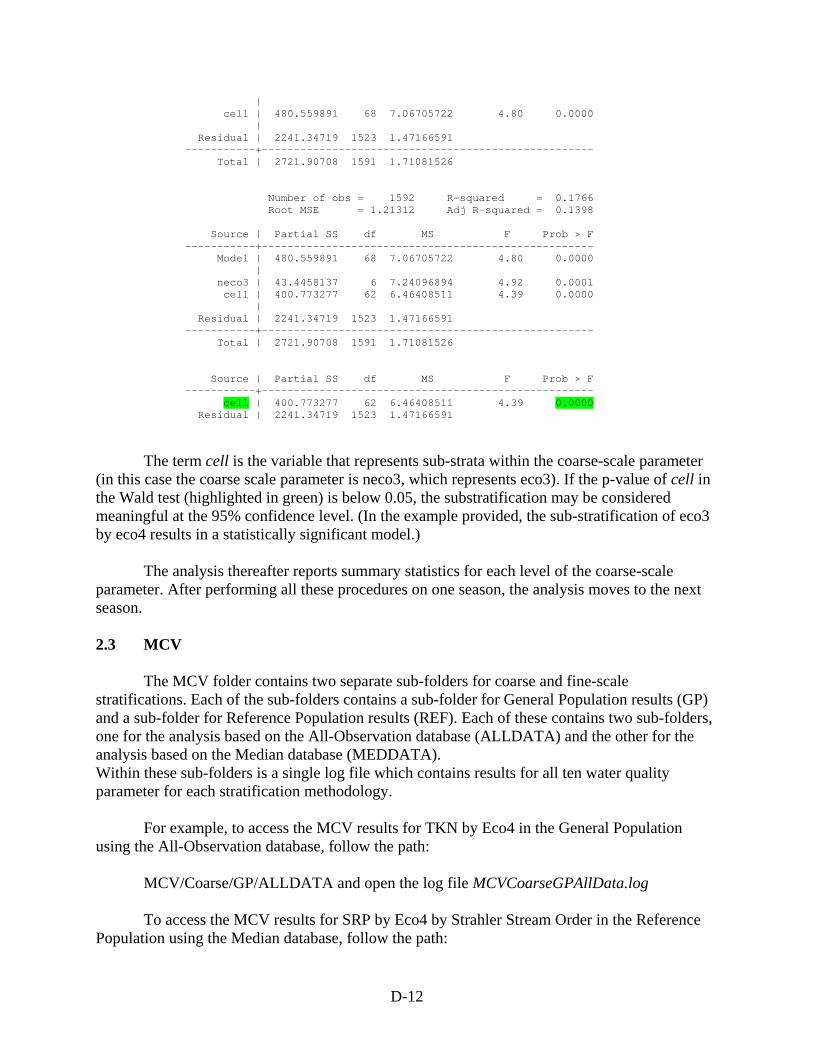
| cell | 480.559891 68 7.06705722 4.80 0.0000 | Residual | 2241.34719 1523 1.47166591 -----------+---------------------------------------------------- Total | 2721.90708 1591 1.71081526 Number of obs = 1592 R-squared = 0.1766 Root MSE = 1.21312 Adj R-squared = 0.1398 Source | Partial SS df MS F Prob > F -----------+---------------------------------------------------- Model | 480.559891 68 7.06705722 4.80 0.0000 | neco3 | 43.4458137 6 7.24096894 4.92 0.0001 cell | 400.773277 62 6.46408511 4.39 0.0000 | Residual | 2241.34719 1523 1.47166591 -----------+---------------------------------------------------- Total | 2721.90708 1591 1.71081526 Source | Partial SS df MS F Prob > F -----------+---------------------------------------------------- cell | 400.773277 62 6.46408511 4.39 0.0000 Residual | 2241.34719 1523 1.47166591
The term cell is the variable that represents sub-strata within the coarse-scale parameter
(in this case the coarse scale parameter is neco3, which represents eco3). If the p-value of cell in the Wald test (highlighted in green) is below 0.05, the substratification may be considered meaningful at the 95% confidence level. (In the example provided, the sub-stratification of eco3 by eco4 results in a statistically significant model.)
The analysis thereafter reports summary statistics for each level of the coarse-scale parameter. After performing all these procedures on one season, the analysis moves to the next season. 2.3 MCV
The MCV folder contains two separate sub-folders for coarse and fine-scale stratifications. Each of the sub-folders contains a sub-folder for General Population results (GP) and a sub-folder for Reference Population results (REF). Each of these contains two sub-folders, one for the analysis based on the All-Observation database (ALLDATA) and the other for the analysis based on the Median database (MEDDATA). Within these sub-folders is a single log file which contains results for all ten water quality parameter for each stratification methodology.
For example, to access the MCV results for TKN by Eco4 in the General Population using the All-Observation database, follow the path:
MCV/Coarse/GP/ALLDATA and open the log file MCVCoarseGPAllData.log
To access the MCV results for SRP by Eco4 by Strahler Stream Order in the Reference Population using the Median database, follow the path:
D-12

MCV/Fine/REF/MEDDATA and open the log file MCVFineREFMedData.log
The coarse scale log files report the MCV, COE and total observations for each nutrient,
for a number of stratification methodologies, for each season. The log files are self-explanatory. A sample output is provided below. XXXXXXXXXXXXXXXXXXXXXXXXXXXXXXXXXXXXXXXXXXXXXXXXXXXXXXXXXXXXXXXXXXXXXX XXXXXXXXXXXXXXXXXXXXXXXXXXXXXXXXXXXXXXXXXXXXXXXXXXXXXXXXXXXXXXXXXXXXXX XXXXXXXXXXXXXXXXXXXXXXXXXXXXXXXXXXXXXXXXXXXXXXXXXXXXXXXXXXXXXXXXXXXXXX MCV ANALYSIS FOR GENERAL POPULATION, ALL DATA NUTRIENT = TOTALN BY Level 3 Ecoregion BY SEASON XXXXXXXXXXXXXXXXXXXXXXXXXXXXXXXXXXXXXXXXXXXXXXXXXXXXXXXXXXXXXXXXXXXXXX XXXXXXXXXXXXXXXXXXXXXXXXXXXXXXXXXXXXXXXXXXXXXXXXXXXXXXXXXXXXXXXXXXXXXX XXXXXXXXXXXXXXXXXXXXXXXXXXXXXXXXXXXXXXXXXXXXXXXXXXXXXXXXXXXXXXXXXXXXXX ************************************************************************************************* NUTRIENT = TOTALN, SEASON = ALL SEASONS, by Level 3 Ecoregion MCV = 1.472456999216334 COE (Log Transformed) = .4315597138630014 TOTAL OBSERVATIONS = 4830 ************************************************************************************************* ************************************************************************************************* NUTRIENT = TOTALN, SEASON = WINTER, by Level 3 Ecoregion MCV = 1.086934706932231 COE (Log Transformed) = .3559982722827028 TOTAL OBSERVATIONS = 1779 ************************************************************************************************* ************************************************************************************************* NUTRIENT = TOTALN, SEASON = RUNOFF, by Level 3 Ecoregion MCV = 1.144742222687749 COE (Log Transformed) = .5330003741207156 TOTAL OBSERVATIONS = 1716 ************************************************************************************************* ************************************************************************************************* NUTRIENT = TOTALN, SEASON = GROWING, by Level 3 Ecoregion MCV = 2.010365373877689
D-13

COE (Log Transformed) = .423718064817054 TOTAL OBSERVATIONS = 1335 *************************************************************************************************
The introductory comment enclosed between two triple lines of “X”s indicates which
nutrient and stratification methodology are being analysed and also specifies which population (general or reference) and database (All-Observations or Median) are analyzed. The MCV and COE results are thereafter reported for each season, enclosed between lines of “*”s. Specific results may be located by using the appropriate word searches within a text editor or by scrolling through the log file. The analyses were processed in the following order: mtmcvc TOTALN eco3 mtmcvc TOTALN eco4 mtmcvc TOTALN geco mtmcvc TOTALN sfname mtmcvc TOTALN strahler mtmcvc TOTALN strahgroup mtmcvc TKN eco3 mtmcvc TKN eco4 mtmcvc TKN geco mtmcvc TKN sfname mtmcvc TKN strahler mtmcvc TKN strahgroup mtmcvc NO3+NO2 eco3 mtmcvc NO3+NO2 eco4 mtmcvc NO3+NO2 geco mtmcvc NO3+NO2 sfname mtmcvc NO3+NO2 strahler mtmcvc NO3+NO2 strahgroup mtmcvc TOTALP eco3 mtmcvc TOTALP eco4 mtmcvc TOTALP geco mtmcvc TOTALP sfname mtmcvc TOTALP strahler mtmcvc TOTALP strahgroup mtmcvc SRP eco3 mtmcvc SRP eco4 mtmcvc SRP geco mtmcvc SRP sfname mtmcvc SRP strahler mtmcvc SRP strahgroup mtmcvc TDP eco3 mtmcvc TDP eco4 mtmcvc TDP geco mtmcvc TDP sfname mtmcvc TDP strahler mtmcvc TDP strahgroup
D-14

mtmcvc AMMONIA eco3 mtmcvc AMMONIA eco4 mtmcvc AMMONIA geco mtmcvc AMMONIA sfname mtmcvc AMMONIA strahler mtmcvc AMMONIA strahgroup mtmcvc BNCHLOR-A eco3 mtmcvc BNCHLOR-A eco4 mtmcvc BNCHLOR-A geco mtmcvc BNCHLOR-A sfname mtmcvc BNCHLOR-A strahler mtmcvc BNCHLOR-A strahgroup mtmcvc TURB-JTU eco3 mtmcvc TURB-JTU eco4 mtmcvc TURB-JTU geco mtmcvc TURB-JTU sfname mtmcvc TURB-JTU strahler mtmcvc TURB-JTU strahgroup mtmcvc TURB-NTU eco3 mtmcvc TURB-NTU eco4 mtmcvc TURB-NTU geco mtmcvc TURB-NTU sfname mtmcvc TURB-NTU strahler mtmcvc TURB-NTU strahgroup
The fine-scale analysis follows the same format as the coarse-scale log files. The fine-scale analyses were processed in the following order: mtmcvf TOTALN eco3 strahler mtmcvf TOTALN eco3 strahgroup mtmcvf TOTALN eco3 sfname mtmcvf TOTALN eco4 strahler mtmcvf TOTALN eco4 strahgroup mtmcvf TOTALN eco4 sfname mtmcvf TOTALN geco strahler mtmcvf TOTALN geco strahgroup mtmcvf TOTALN geco sfname mtmcvf TKN eco3 strahler mtmcvf TKN eco3 strahgroup mtmcvf TKN eco3 sfname mtmcvf TKN eco4 strahler mtmcvf TKN eco4 strahgroup mtmcvf TKN eco4 sfname mtmcvf TKN geco strahler mtmcvf TKN geco strahgroup mtmcvf TKN geco sfname mtmcvf NO3+NO2 eco3 strahler mtmcvf NO3+NO2 eco3 strahgroup mtmcvf NO3+NO2 eco3 sfname
D-15
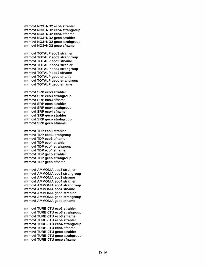
mtmcvf NO3+NO2 eco4 strahler mtmcvf NO3+NO2 eco4 strahgroup mtmcvf NO3+NO2 eco4 sfname mtmcvf NO3+NO2 geco strahler mtmcvf NO3+NO2 geco strahgroup mtmcvf NO3+NO2 geco sfname mtmcvf TOTALP eco3 strahler mtmcvf TOTALP eco3 strahgroup mtmcvf TOTALP eco3 sfname mtmcvf TOTALP eco4 strahler mtmcvf TOTALP eco4 strahgroup mtmcvf TOTALP eco4 sfname mtmcvf TOTALP geco strahler mtmcvf TOTALP geco strahgroup mtmcvf TOTALP geco sfname mtmcvf SRP eco3 strahler mtmcvf SRP eco3 strahgroup mtmcvf SRP eco3 sfname mtmcvf SRP eco4 strahler mtmcvf SRP eco4 strahgroup mtmcvf SRP eco4 sfname mtmcvf SRP geco strahler mtmcvf SRP geco strahgroup mtmcvf SRP geco sfname mtmcvf TDP eco3 strahler mtmcvf TDP eco3 strahgroup mtmcvf TDP eco3 sfname mtmcvf TDP eco4 strahler mtmcvf TDP eco4 strahgroup mtmcvf TDP eco4 sfname mtmcvf TDP geco strahler mtmcvf TDP geco strahgroup mtmcvf TDP geco sfname mtmcvf AMMONIA eco3 strahler mtmcvf AMMONIA eco3 strahgroup mtmcvf AMMONIA eco3 sfname mtmcvf AMMONIA eco4 strahler mtmcvf AMMONIA eco4 strahgroup mtmcvf AMMONIA eco4 sfname mtmcvf AMMONIA geco strahler mtmcvf AMMONIA geco strahgroup mtmcvf AMMONIA geco sfname mtmcvf TURB-JTU eco3 strahler mtmcvf TURB-JTU eco3 strahgroup mtmcvf TURB-JTU eco3 sfname mtmcvf TURB-JTU eco4 strahler mtmcvf TURB-JTU eco4 strahgroup mtmcvf TURB-JTU eco4 sfname mtmcvf TURB-JTU geco strahler mtmcvf TURB-JTU geco strahgroup mtmcvf TURB-JTU geco sfname
D-16

mtmcvf TURB-NTU eco3 strahler mtmcvf TURB-NTU eco3 strahgroup mtmcvf TURB-NTU eco3 sfname mtmcvf TURB-NTU eco4 strahler mtmcvf TURB-NTU eco4 strahgroup mtmcvf TURB-NTU eco4 sfname mtmcvf TURB-NTU geco strahler mtmcvf TURB-NTU geco strahgroup mtmcvf TURB-NTU geco sfname mtmcvf BNCHLOR-A eco3 strahler mtmcvf BNCHLOR-A eco3 strahgroup mtmcvf BNCHLOR-A eco3 sfname mtmcvf BNCHLOR-A eco4 strahler mtmcvf BNCHLOR-A eco4 strahgroup mtmcvf BNCHLOR-A eco4 sfname mtmcvf BNCHLOR-A geco strahler mtmcvf BNCHLOR-A geco strahgroup mtmcvf BNCHLOR-A geco sfname 2.4 SEASONS
The SEASONS folder contains two separate sub-folders for coarse and fine-scale stratifications. Each of the sub-folders contains a sub-folder for General Population results (GP) and a sub-folder for Reference Population results (REF). Each of these contains two sub-folders, one for the analysis based on the All-Observation database (ALLDATA) and the other for the analysis based on the Median database (MEDDATA). Within these sub-folders are sub-folders for the ten water quality parameters, each containing a subfolder named ECO3, which contains a log file with the results of tests for differences in seasonal concentrations in each level III ecoregion.
For example, to access the seasonal testing results for ECO3 for TKN in the General Population using the All-Observation database, follow the path: SEASONS\GP\ALLDATA\TKN\ECO3 and open the log file TKNeco3GPAll.log
In the log files, each level III ecoregion is considered one at a time. Summary statistics are first presented for each season. The Kruskal Wallis test is then performed to test for significant differences between the median nutrient concentrations across the different seasons. A non-parametric multiple comparison test is then performed to determine which specific seasons may be considered different from each other. ANOVA and multiple comparisons of seasonal means based on the Bonferroni adjustment are thereafter presented. The interpretation of these tests has been described in Section 2.2 of this appendix and is not repeated here. The analysis then proceeds to the next level III ecoregion.
(Note: The ALLDATA analyses present results only for specific seasons (Winter, Runoff, Growing) whereas the MEDDATA report result for specific seasons as well as for all seasons. This difference in formats is due to differences in the structures of the two databases.)
D-17

2.5 STRAHDIST
The STRAHDIST folder contains two sub-folders, one for station-level analysis (STATION) and the other for observation-level analysis (OBS).
Each of the subfolders has ten subfolders for each of the water quality parameters. Within them is a further subfolder called ECO3, representing the analysis for level III ecoregions. (The analysis is only presented for level III ecoregions for all seasons.)
For example, to access the Strahler stream order distributional analysis for TKN at the station level for level III ecoregions, follow the path: STRAHDIST\STATION\TKN\ECO3 and open the log file: TKNeco3stationstrahdist.log
In the log files, each level III ecoregion is considered one at a time. A tabulation of stream order in the general and reference population in the ecoregion is first presented. The Pearson chi-square test is then presented to assess whether the distribution of stream order in the general and reference populations may be considered equal in that ecoregion.
D-18

An example of this test is provided below: _________________________________________________________________ PEARSON CHI SQUARE TEST for Nutrient=TKN, Level 3 Ecoregion = Middle Rockies for REF and NON-REF ST > ATIONS | REF STRAHLER | N Y | Total -----------+----------------------+---------- 1 | 99 0 | 99 | 15.97 0.00 | 15.40 -----------+----------------------+---------- 2 | 163 10 | 173 | 26.29 43.48 | 26.91 -----------+----------------------+---------- 3 | 160 8 | 168 | 25.81 34.78 | 26.13 -----------+----------------------+---------- 4 | 79 1 | 80 | 12.74 4.35 | 12.44 -----------+----------------------+---------- 5 | 65 0 | 65 | 10.48 0.00 | 10.11 -----------+----------------------+---------- 6 | 25 4 | 29 | 4.03 17.39 | 4.51 -----------+----------------------+---------- 7 | 26 0 | 26 | 4.19 0.00 | 4.04 -----------+----------------------+---------- 8 | 3 0 | 3 | 0.48 0.00 | 0.47 -----------+----------------------+---------- Total | 620 23 | 643 | 100.00 100.00 | 100.00 Pearson chi2(7) = 20.3102 Pr = 0.005 REJECT THE HYPOTHESIS THAT STRAHLER DISTRIBUTION IS EQUAL IN REF AND NON-REF STATIONS
The distribution of Strahler stream order may be considered to be different in the general and reference population with 95% statistical confidence if the highlighted p-value is less than 0.05. However, the output translates the result of this test into a direct statement of whether the distributions are different.
The analysis also performs the Kruskal Wallis test, and presents histograms of the stream order distribution in the general and reference population with a superimposed normal distribution curve for each level III ecoregion. An example of the graphical output is presented in Figure D-5. The histogram marked “N” refers to the non-reference population and “Y” refers to the reference population.
D-19

Figure D-5: Example of Histograms in STRAHDIST Analysis Grouped By Reference Status -- STATIONS
Frac
tion
Nutrient=TKN, Level 3 Ecoregion= Middle RockiesSTRAHLER
N
1 80
.434783
Y
1 8
D-20