Median Unbiased Estimation of Coefficient Variance in a Time-Varying Parameter … ·...

Median Unbiased Estimation of Coefficient Variance in a Time-Varying Parameter Model

James H. STOCK and Mark W. WATSON

This article considers inference about the variance of coefficients in time-varying parameter models with stationary regressors. The Gaussian maximum likelihood estimator (MLE) has a large point mass at 0. We thus develop asymptotically median unbiased estimators and asymptotically valid confidence intervals by inverting quantile functions of regression-based parameter stability test statistics, computed under the constant-parameter null. These estimators have good asymptotic relative efficiencies for small to moderate amounts of parameter variability. We apply these results to an unobserved components model of trend growth in postwar U.S. per capita gross domestic product. The MLE implies that there has been no change in the trend growth rate, whereas the upper range of the median-unbiased point estimates imply that the annual trend growth rate has fallen by 0.9% per annum since the 1950s.

KEY WORDS: Stochastic coefficient model; Structural time series model; Unit moving average root; Unobserved components.

1. INTRODUCTION

Since its introduction in the early 1970s by Cooley and Prescott (1973a,b, 1976), Rosenberg (1972, 1973), and Sar- ris (1973), the time-varying parameter (TVP), or "stochastic coefficients," regression model has been used extensively in empirical work, especially in forecasting applications. Chow (1984), Engle and Watson (1987), Harvey (1989), Nichols and Pagan (1985), Pagan (1980), and Stock and Watson (1996) have provided references and discussion of this model. The appeal of the TVP model is that by permit- ting the coefficients to evolve stochastically over time, it can be applied to time series models with parameter instability.

The TVP model considered in this article is

yt = 3itXt + ut, (1)

,3t /3t-l + vt, (2)

a(L)ut = Et, (3)

and

vt = Tvt, where vt = B(L)qt, (4)

where {(yt,Xt),t = 1,... ,T} are observed, Xt is an exogenous k-dimensional regressor, /3t is a k x 1 vector of unobserved time-varying coefficients, T is a scalar, a(L) is a scalar lag polynomial, B(L) is a k x k matrix lag polynomial, and Et and qt are serially and mutually uncorrelated mean 0 random disturbances. (Additional technical conditions used for the asymptotic results are given in Section 2, where we also discuss restrictions on B(L) and E(rqtqr) that are sufficient to identify the scale factor T.) An im- portant special case of this model is when Xt = 1 and B(L) = 1; following Harvey (1985), we refer to this case as the "local-level" unobserved components model.

James H. Stock is Professor of Political Economy, Kennedy School of Government, Harvard University, Cambridge, MA 02138, and Research Associate at the National Bureau of Economic Research (NBER). Mark W. Watson is Professor of Economics and Public Affairs, Woodrow Wilson School, Princeton University, Princeton, NJ 08544, and Research Associate at the NBER. The authors thank Bruce Hansen, Andrew Harvey and two referees for comments on an earlier draft, and Lewis Chan and Jonathan Wright for research assistance. This research was supported in part by National Science Foundation grant SBR-9409629.

We consider the problem of estimation of the scale parameter r. If (as is common) et and nt are assumed to be jointly normal and independent of {Xt, t-1) . . .; T}, then the parameters of (1)-(4) can be estimated by maximum likelihood implemented by the Kalman filter. However, the maximum likelihood estimator (MLE) has the undesirable property that if r is small, then it has point mass at 0. In the case Xt - 1, this is related to the so-called pile-up problem in the first-order moving average [MA( 1)] model with a unit root (Sargan and Bhargava 1983; Shephard and Harvey 1990). In the general TVP model (1)-l4), the pile-up probability depends on the properties of Xt and can be large. The pile-up probability is a particular problem when 7 is small and thus is readily mistaken for 0. Arguably, small values of r are appropriate for many empirical applications; indeed, if 7 is large, then the distribution of the MLE can be approximated by conventional T1/2-asymptotic normality, but Monte Carlo evidence suggests that this approximation is poor in many cases of empirical interest. (See Davis and Dunsmuir 1996 and Shephard 1993 for discussions in the case of Xt = 1.)

We thus focus on the estimation of r when it is small. In particular, we consider the nesting

r = A/T. (5)

Order of magnitude calculations suggest that this might be an appropriate nesting for certain empirical problems of interest, such as estimating stochastic variation in the trend component in the growth rate of U.S. real gross domestic product (GDP), as we discuss in Section 4. This is also the nesting used to obtain local asymptotic power functions of tests of 7r 0, a fact suggesting that if the researcher is in a region in which tests yield ambiguous conclusions about the null hypothesis 7r 0, then the nesting (5) is appropriate.

The main contribution of this article is the development of asymptotically median unbiased estimators of A and asymptotically valid confidence intervals for A in the model (1)-(5). These are obtained by inverting asymptotic quantile functions of statistics that test the hypothesis A = 0. The

? 1998 American Statistical Association Journal of the American Statistical Association

March 1998, Vol. 93, No. 441, Theory and Methods

349

350 Journal of the American Statistical Association, March 1998

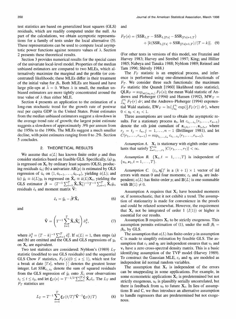
test statistics are based on generalized least squares (GLS) residuals, which are readily computed under the null. As part of the calculations, we obtain asymptotic representations for a family of tests under the local alternative (5). These representations can be used to compute local asymptotic power functions against nonzero values of A. Section 2 presents these theoretical results.

Section 3 provides numerical results for the special cases of the univariate local-level model. Properties of the median unbiased estimators are compared to two MLEs, which alternatively maximize the marginal and the profile (or concentrated) likelihoods; these MLEs differ in their treatment of the initial value for 3t. Both MLEs are biased and have large pile-ups at A = 0. When A is small, the median unbiased estimators are more tightly concentrated around the true value of A than either MLE.

Section 4 presents an application to the estimation of a long-run stochastic trend for the growth rate of postwar real per capita GDP in the United States. Point estimates from the median unbiased estimators suggest a slowdown in the average trend rate of growth; the largest point estimate suggests a slowdown of approximately .9% per annum from the 1950s to the 1990s. The MLEs suggest a much smaller decline, with point estimates ranging from 0 to .2%. Section 5 concludes.

2. THEORETICAL RESULTS

We assume that a(L) has known finite order p and thus consider statistics based on feasible GLS. Specifically, (a) Yt is regressed on Xt by ordinary least squares (OLS), produc- ing residuals fit; (b) a univariate AR(p) is estimated by OLS regression of fit on (1,It-i,... , yielding &(L); and (c) t = &(L)yt is regressed on Xt &(L)Xt, yielding the GLS estimator ,3 - (T-1 Et=L1 XtX ) t1T-1 t=1 xy, residuals et and moment matrix V:

et = It-3'Xt (6)

and

V = (T-1 E tk &2 (7)

where &2 = (T - k)-1 ET= E2. If a(L) 1, then steps (a) and (b) are omitted and the OLS and GLS regressions of Yt on Xt are equivalent.

Two test statistics are considered: Nyblom's (1989) LT statistic (modified to use GLS residuals) and the sequential GLS Chow F statistics, FT(s)(O < s < 1), which test for a break at date [Ts], where [.] denotes the greatest lesser integer. Let SSRt1,t2 denote the sum of squared residuals from the GLS regression of jt onto Xt over observations tl < t < t2, and let CT(S) = T-1/2 E[Ts] Xtet. The LT and FT statistics are

T

LT-T-1 Z (T(t/T)V-1 T(t/T) (8) t= 1

and

FT(s) = (SSRl,T- SSRl,[Ts] - SSRrTs]+1,T)

? [k(SSRl,[Ts] + SSR[TS]+l,T)/(T - k)]. (9)

(For other tests in versions of this model, see Franzini and Harvey 1983; Harvey and Streibel 1997; King; and Hillier 1985; Nabeya and Tanaka 1988; Nyblom 1989; Reinsel and Tam 1996; Shively 1988.)

The FT statistic is an empirical process, and inference is performed using one-dimensional functionals of FT. We consider three such functionals: the maximum FT statistic (the Quandt [1960] likelihood ratio statistic), QLRT = supSE(S,S1) FT(s); the mean Wald statistic of An- drews and Ploberger (1994) and Hansen (1992), MWT =

f Z FT(r) dr; and the Andrews-Ploberger (1994) exponential Wald statistic, EWT = ln{f1 exp( FT(r)) dr}, where O < so < SI < 1.

Three assumptions are used to obtain the asymptotic results. For a stationary process Zt, let ci ...i.(r, ..rn-1) denote the nth joint cumulant of zi1t1,...)zintn, where rj = tj-tn,j = 1, . ..,n-1 (Brillinger 1981), and let C(ri,..., rn-1) = Supil,.,in Cil ... in(rl, * * rn-1).

Assumption A. Xt is stationary with eighth order cumulants that satisfy ,.rJ I C(rI,... ,r7) < 00

Assumption B. {Xt, t = 1,... ,T} is independent of {Ut, Vt, t1, ...,T}.

Assumption C. (Ct, r)' is a (k + 1) x 1 vector of iid errors with mean 0 and four moments; Et and rt are independent; a(L) has finite-order p; and B(L) is one-summable with B(1) 34 0.

Assumption A requires that Xt have bounded moments or, if nonstochastic, that it not exhibit a trend. The assumption of stationarity is made for convenience in the proofs and could be relaxed somewhat. However, the requirement that Xt not be integrated of order 1 (I(1)) or higher is essential for our results.

Assumption B requires Xt to be strictly exogenous. This assumption permits estimation of (1), under the null f3t 3o0, by GLS.

The assumption that a(L) has finite-order p in assumption C is made to simplify estimation by feasible GLS. The assumption that Et and rt are independent ensures that ut and vt have a zero cross-spectral density matrix. This is a basic identifying assumption of the TVP model (Harvey 1989). To construct the Gaussian MLE, Et and rt are modeled as independent iid normal random variables.

The assumption that Xt is independent of the errors can be unappealing in some applications. For example, in some econometric applications Xt is predetermined but not strictly exogenous, ut is plausibly serially uncorrelated, but there is feedback from Ut to future Xt. In lieu of assumptions B and C, we thus introduce an alternative assumption to handle regressors that are predetermined but not exogenous.

Stock and Watson: Time-Varying Parameters 351

Assumption D. (6t,4)' is a (k + 1) x 1 vector of iid errors with mean 0 and four moments; Et and nt are independent; a(L) = 1; B(L) is one-summable with B(1) 74 0; nIt is independent of {Xt, Xt?l, Xt?2,.. .}; and ut is independent of {Xt, Xti l, Xt-2, ..

This permits feedback from ut to future Xt, but not from vt to Xt, and thus rules out Xt containing lagged Yt when A#o.

Our main theoretical results are given in the following theorem. Let ">" denote weak convergence on D[0, 1], let W1 and W2 be independent standard Brownian mo- tions on [0, ]k, and let F = E{ [a(L)Xt] [a(L)Xt]'}, l =

B(1)E(7qntq)B(1)', and D= r1/2n1/2/ Theorem 1. Let Yt obey (1)-(5), and suppose either that

assumptions A, B, and C hold or that assumptions A and D hold. Then

a. V-1/2(T X hO, where h0(s) = hA(s)-shA(1), where hA (s) = Wi (s) + AD fs W2 (r) dr;

b. LT X f0 h?(s)'h? (s) ds; and c. FT => F*, where F*(s) = h0(s)'h?(s)/(ks(1 - s)).

The proof is given in the Appendix. Limiting representations of the QLR, mean Wald, and

exponential Wald statistics are obtained from part (c) of Theorem I and the continuous mapping theorem. Thus QLRT ?I sup,,<,<,1 F*(s), MWT f> JS F*(r) dr, and EWT X> ln{<1 exp( 2F* (r))dr}. Note that the limiting representation for LT can be written as LT =X k f (r(1 - r))F* (r) dr.

When A = 0, the process hO is a k-dimensional Brown- ian bridge, and the representations for the statistics LT and FT reduce to their well-known null representations as functionals of a Brownian bridge (Andrews and Ploberger 1994; Nabeya and Tanaka 1988; Nyblom 1989).

When A 7& 0, the limiting distributions of LT and FT depend on two parameters, A and D. The limiting representations in Theorem 1 are used for three purposes: to compute local asymptotic power functions, to construct median unbiased estimators of A, and to construct asymptotically valid confidence intervals for A. To do so, D must either be known or be consistently estimable, so that asymptotically A is the only unknown parameter entering these distributions.

The determination of D raises issues of identification and modeling strategy. Evidently a(L) and var(ct) are not separately identified, but this is resolved without loss of generality by adopting the normalization ao 0 1. Similarly, for standard reasons associated with moving average models, B(L) and Enitn' are not separately identified; we thus adopt the conventional assumptions that Bo = Ik and the roots of IB(z) are outside the unit circle. Even with these assumptions, however, inspection of (1)-(5) reveals that A and Q? are not separately identified: The parameter combinations (A, Q) = (A, Q) and (A, Q) = (1, >2) are observationally equivalent for fixed (A, Q).

When k = 1, this identification problem can be solved without loss of generality by adopting an arbitrary normal-

ization. Henceforth, when k = 1, we thus set D = 1. When Xt = 1, under this normalization, A is T times the ratio of the long-run standard deviation of A/3t to the long run standard deviation of ut.

When k > 1, Ql is identified upon making a single suit- able normalization; for example, that the trace of -Q is unity. However, the local-to-O variation in A/3t makes it impossi- ble to estimate the free elements of Q consistently without further restrictions. In this case two types of further restrictions suggest themselves. First, Q may be set equal to a prespecified constant matrix chosen by the researcher in a manner appropriate for the specific empirical model under study. Second, Q may be parameterized as a function of r and a 2 (which are consistently estimable). As in the k = 1 case, a convenient parameterization sets Q - ar2Y-1, for this implies that D = Ik. This choice of Q implies that the regression coefficients evolve as mutually independent random walks after rotating the regressors so that they are mutually uncorrelated. This is the parameterization used by Nyblom (1989) in his development of the LMPI test for A 0 O. From a computational perspective, this assumption is attractive because it simplifies the calculation of median unbiased estimators of A and the construction of confidence intervals. From a modeling perspective, the restriction is arguably appealing because it makes the magnitude of the time variation comparable across variables when measured in standard deviation units (or, for general a(L) and /(L), long-run standard deviation units). With the additional restrictions a(L) =1 and B(L) = 1, this restriction was used by Stock and Watson (1996) in their investigation of time variation in empirical macroeconomic relationships. Whether this assumption is desirable for general Xt is a matter of modeling strategy in a particular empirical application.

2.1 Local Asymptotic Power

The representations can be used to compute the distribution of the tests under the local alternative (5) and thus to compute the local asymptotic power of tests of the null T = 0. The various test statistics have limiting representations under the local alternative that are qualitatively similar. This is interesting, because the FT-based statistics are typically motivated by considering the single break model, whereas Nyblom (1989) derived the LT statistic as the LMPI test statistic for the seemingly rather different Gaus- sian TVP model.

2.2 Median Unbiased Estimation of A

Median unbiased estimators of A can be computed from LT or from a scalar functional of FT. Consider, for example, the scalar functional g(FT), which is assumed to be continuous. By the continuous mapping theorem, g(FT) =>

g(F*), the distribution of which depends on A and D. Let mD(A) denote the median of g(F*) as a function of A for a given matrix of nuisance parameters D. Suppose that mn(.) is monotone increasing and continuous in A. Then the inverse function mj-1 exists, and for D known, A can be es-


timated by

=mD(g(FT)). (10)

Asymptotically, A0 A mj -(g(F*)). By construction, Pr[% < A] - Pr[mj1(g(F*)) < Al = Pr[g(F*) < mD(A)] .5, so A9 is asymptotically median unbiased.

In practice D is not known, so the estimator (10) is in- feasible. However, as discussed earlier, D generally can be consistently estimated for a given choice of Q. If in addition mjn (.) is continuous in D (which it is for the functionals considered in this article), then (10) can be computed with D replaced by a consistent estimator D, and the same asymptotic distribution obtains. Note, however, that this is computationally cumbersome, as it requires computing the inverse median function mn;1 (.) for every estimate D under consideration. (However, some simplifications are possible because, as pointed out by a referee, the distribution of the test statistics depends only on the eigenvalues of D.) When Q is chosen so that D= Ik, the limiting distributions of LT and FT depend only on A and k under the local alternative.

It would be of interest to obtain theoretical results com- paring the efficiency of median-unbiased estimators based on the various functionals of FT. However, the limiting distributions are nonstandard and do not appear to have any simple relation to each other. Thus these efficiency comparisons are undertaken numerically and are reported in the next section.

2.3 Confidence Intervals for A

Suppose that D = Ik, in which case the local asymptotic representatiorns in Theorem 1 depend only on A and k. For a given scalar test statistic, its representation can then be used to compute a family of asymptotic 5% critical values of tests of A = A0 against a two-sided alternative, and in turn these critical values can be used to construct the set of A0 that are not rejected. This set constitutes a 95% confidence set for A0. This process of inverting the test statistic can be

0

0

0? /j

O X,

(D

0 0 5 10 15 20 25 30

Figure 1. Asymptotic Power Functions ot 5% Tests otTr = 0 Against Alternatives w = A/T. - , envelope; ,L; -,MW; ,EW; -- -, QLR; ,P01(7J; ---, P01(17J.

done graphically by the method of confidence belts or by interpolation of a lookup table. The details parallel those for construction of confidence intervals for autoregressive roots local to unity (Stock 1991) and are omitted.

3. NUMERICAL RESULTS FOR THE UNIVARIATE LOCAL-LEVEL MODEL

In the univariate of local-level model, Xt 1 and B(L) = 1, so that yt is the sum of an I(0) component and an independent random walk, which under the parameterization (5) has a small disturbance variance. In this model AYt follows a moving average (MA) process, with largest MA root (1 - A/T)-> + o(T-1). In this section we first compare numerically the power of the tests in Section 2 and of some other previously proposed tests against the local alternative, then turn to an analysis of the properties of median unbiased estimators. All computations of asymptotic distributions are based on simulation of the limiting representations, with T = 500 and 5,000 Monte Carlo replications.

3.1 Asymptotic Power of Tests

A great deal of work has been on tests of A = 0 in the local-level model and of a unit MA root in the related MA(1) model (see Nyblom and Makelainen 1983; Saikko- nen and Luukonen 1993; Shively 1988; Stock 1994; Tanaka 1990). In addition to the tests discussed in Section 2, local power functions are computed for two point-optimal invariant (POI) tests (Saikkonen and Luukkonen 1993; Shive- ly 1988), for A = 7 and A = 17, denoted by P01(7) and P0(17). As a basis of comparison, we also computed the asymptotic Gaussian power envelope.

Asymptotic powers of various 5% tests are summarized in Figure 1. Evidently, for small values of A all tests ef- fectively lie on the asymptotic Gaussian power envelope. For more distant alternatives, the MW and L tests lose power and, to a lesser degree, so do the EW and QLR. The asymptotic power functions of the EW and QLR tests are essentially indistinguishable, consistent with findings else- where (Andrews, Lee, and Ploberger 1996; Stock and Wat- son 1996) that these tests perform similarly.

3.2 Estimators of A

Each of the tests examined in Figure 1 has a power function that depends only on A and has a median function that is monotone and continuous in A. Asymptotically median unbiased estimators of A based on each of these tests thus can be constructed as described in Section 2. In addition, results are reported for two versions of the Gaussian MLE that differ in their assumptions concerning the initial value of 1o. The first estimator, the maximum profile (or concentrated) likelihood estimator (MPLE), treats Q0 as an unknown nuisance parameter that is concentrated out of the likelihood. The second estimator, the maximum marginal likelihood estimator (MMLE), treats \ Io as a N(, T ) random variable that is independent of {Ut, vt, t =1 ,... ., T}, so that f0o is integrated out of the likelihood. When i oc, this produces the "diffuse prior" likelihood function (see Shephard 1993


Table 1. Pile-Up Probability That A = 0 for MLEs and Various Median-Unbiased Estimators

A MPLE MMLE L MW EW QLR P01(7) P01(17)

0 .96 .66 .50 .50 .50 .50 .50 .50 1 .91 .60 .47 .47 .47 .46 .47 .47 2 .88 .57 .42 .42 .42 .43 .44 .43 3 .81 .47 .34 .34 .34 .35 .35 .37 4 .72 .40 .28 .28 .29 .29 .29 .30 5 .65 .35 .24 .24 .24 .24 .24 .26 6 .56 .28 .19 .19 .19 .19 .18 .20 7 .48 .24 .15 .16 .16 .16 .14 .15 8 .42 .19 .13 .13 .13 .13 .12 .13 9 .37 .17 .11 .12 .12 .12 .09 .10

10 .30 .13 .09 .09 .09 .09 .07 .07 12 .24 .09 .06 .07 .07 .06 .05 .05 14 .15 .06 .03 .04 .04 .04 .03 .02 16 .13 .04 .03 .03 .03 .03 .01 .01 18 .09 .03 .02 .03 .02 .02 .01 .01 20 .07 .02 .01 .01 .01 .01 .01 .01 25 .03 .01 .01 .01 .01 .01 .01 .01 30 .01 .01 .01 .01 .01 .01 .01 .01

NOTE: Entries for MPLE and MMLE for A = 0 are from Shepard and Harvey (1990). Entries for other values of A are estimated using 5,000 replications with T = 500. To facilitate the computations, the likelihoods were computed on a discrete grid of 240 equally spaced values of 0 < A < 60, and the MLEs were computed by a search over this grid.

and Shephard and Harvey 1990). The MMLE is equivalent, after reparameterization on a restricted parameter space, to the MA(1) MLE analyzed by Davis and Dunsmuir (1996), and their local-to-unity asymptotic results apply here.

Pile-up probabilities that A is estimated to be exactly 0 are reported in Table 1. The mass of the median unbiased estimators at 0 is similar for all estimators. The pile-up probability for the MPLE remains large as A increases, both in absolute terms (it is above 50% for A < 6) and relative to the median unbiased estimators. As pointed out by Shephard and Harvey (1990), the pile-up probability for the MMLE is smaller than for MPLE.

Cumulative distribution functions of the various estimators for A 5 are plotted in Figure 2. As expected, both

o

O~~~ _

Q / / - n~~~~~~~~

CD

0 /

0 2 4 6 8 10 12 14 16 18 20

oiur /.Cmltv smttcDsrbtoso h asinME an ixMdinUnise stmtrso AWenA= . , PE

--,ML; ,L-,0W ,E ; QR-- 0() o-,P11)

MLEs are biased and median biased. For A = 5, 77% of the mass of the distribution of the MPLE is below the true value and the median is 0; the MMLE performs better, with 64% of its mass below A = 5 and a median bias of approximately -1. The cdfs of the median unbiased estimators are fairly similar to each other, but markedly different than the MLE. One apparent cost of unbiasness is their longer right tail relative to the MLEs.

We compare the estimators by computing their asymptotic relative efficiencies (AREs). Because the distributions are nonnormal and not proportional, conventional methods of computing AREs do not apply. Instead, we mea- sure the ARE of the ith estimator 4rj relative to the MMLE, TMMLE (denoted by AREi,MMLE), as the limit of the ratio of observations TMMLE/Ti needed for Pr[#i c G(r); Tj] = Pr[4MMLE E G(T); TMMLE], where Ti and TMMLE denote the number of observations used to compute $j and TMMLE. The AREs reported here were for the sets G(r) = {x: .5r < x < 1.54}, so Pr[#i c GQr); Ti] = Pr[ITi - TirI < .5Tjr] - pi(Tir), say, and similarly for TMMLE. Using (5), set A TMMLET; then AREj,MMLE = limTMMLE/Ti can be computed by solving Pi(A/AREj,MMLE) = PMMLE(A)-

In general, the ARE depends on A. Table 2 reports these AREs for the MPLE and six me-

dian unbiased estimators for various values of A; all AREs are relative to the MMLE. For example, when A = 4, the ARE of the QLR-based median unbiased estimator, relative to the MMLE, is 1.02, which indicates that in large sam- ples the MMLE requires 1.02 times as many observations as the QLR-based estimator to achieve the same probability of falling in the set G(r). Evidently, MMLE dominates MPLE for all values of A shown and is considerably more efficient for small to moderate values of A. In contrast, the median unbiased estimators perform slightly better than MMLE for small values of A (A < 4) and comparably for moderate

Table 2. Asymptotic Relative Efficiencies of Median-Unbiased Estimators Relative to the MMLE

A MPLE L MW EW QLR P01(7) P01(17)

1 .13 1.00 1.00 1.00 1.00 1.07 1.07 2 .19 1.09 1.07 1.07 .96 1.07 1.02 3 .52 1.08 1.10 1.08 1.04 1.02 .94 4 .62 1.06 1.06 1.06 1.02 1.06 1.00 5 .65 .93 .93 .98 .97 1.11 1.14 6 .71 .94 .92 .99 1.00 1.03 1.08 7 .76 .79 .79 .85 .88 .96 1.04 8 .77 .77 .77 .85 .85 .91 .98 9 .75 .69 .69 .75 .77 .86 .89

10 .80 .65 .65 .71 .74 .80 .80 12 .67 .56 .56 .65 .67 .67 .67 14 .57 .50 .49 .57 .57 .57 .57 16 .50 .42 .42 .49 .50 .50 .50 18 .44 .38 .38 .44 .44 .44 .44 20 .40 .33 .33 .40 .40 .40 .40 25 .32 .28 .28 .32 .32 .32 .32 30 .27 .22 .23 .27 .27 .27 .27

NOTE: The reported AREs are the limiting ratio of the number of observations necessary for the MLE to achieve the same probability of being in the region T ?t .5T as the candidate estimator, as a function of A = TIT, as described in the text. AREs exceeding 1 indicate greater efficiency than the MLE. Entries are estimates based on interpolating probabilities from the values of A shown in column 1. These probabilities were estimated using 5,000 replications and T = 500 for each value of A~.


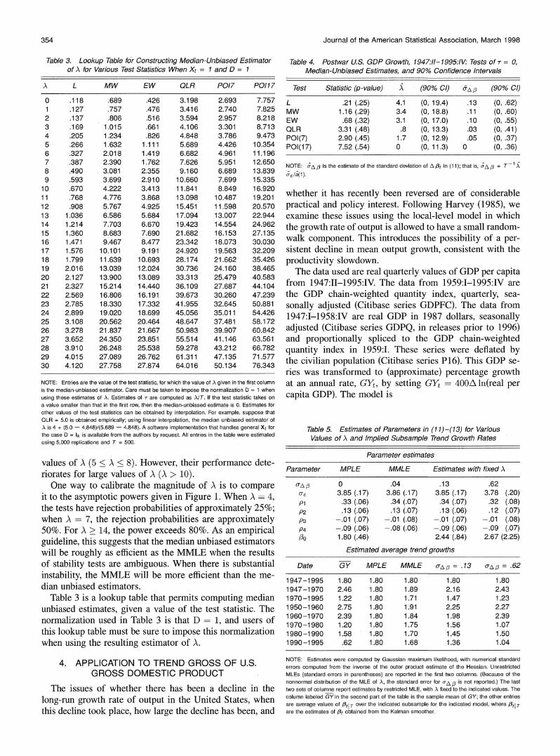
Table 3. Lookup Table for Constructing Median-Unbiased Estimator of A for Various Test Statistics When Xt = 1 and D = 1

A L MW EW QLR P017 P0117

0 .118 .689 .426 3.198 2.693 7.757 1 .127 .757 .476 3.416 2.740 7.825 2 .137 .806 .516 3.594 2.957 8.218 3 .169 1.015 .661 4.106 3.301 8.713 4 .205 1.234 .826 4.848 3.786 9.473 5 .266 1.632 1.111 5.689 4.426 10.354 6 .327 2.018 1.419 6.682 4.961 11.196 7 .387 2.390 1.762 7.626 5.951 12.650 8 .490 3.081 2.355 9.160 6.689 13.839 9 .593 3.699 2.910 10.660 7.699 15.335

10 .670 4.222 3.413 11.841 8.849 16.920 11 .768 4.776 3.868 13.098 10.487 19.201 12 .908 5.767 4.925 15.451 11.598 20.570 13 1.036 6.586 5.684 17.094 13.007 22.944 14 1.214 7.703 6.670 19.423 14.554 24.962 15 1.360 8.683 7.690 21.682 16.153 27.135 16 1.471 9.467 8.477 23.342 18.073 30.030 17 1.576 10.101 9.191 24.920 19.563 32.209 18 1.799 11.639 10.693 28.174 21.662 35.426 19 2.016 13.039 12.024 30.736 24.160 38.465 20 2.127 13.900 13.089 33.313 25.479 40.583 21 2.327 15.214 14.440 36.109 27.687 44.104 22 2.569 16.806 16.191 39.673 30.260 47.239 23 2.785 18.330 17.332 41.955 32.645 50.881 24 2.899 19.020 18.699 45.056 35.011 54.426 25 3.108 20.562 20.464 48.647 37.481 58.172 26 3.278 21.837 21.667 50.983 39.907 60.842 27 3.652 24.350 23.851 55.514 41.146 63.561 28 3.910 26.248 25.538 59.278 43.212 66.782 29 4.015 27.089 26.762 61.311 47.135 71.577 30 4.120 27.758 27.874 64.016 50.134 76.343

NOTE: Entries are the value of the test statistic, for which the value of A given in the first column is the median-unbiased estimator. Care must be taken to impose the normalization D = 1 when using these estimates of A. Estimates of T are computed as AIT. If the test statistic takes on a value smaller than that in the first row, then the median-unbiased estimate is 0. Estimates for other values of the test statistics can be obtained by interpolation. For example, suppose that QLR = 5.0 is obtained empirically; using linear interpolation, the median unbiased estimator of A is 4 + (5.0 - 4.848)/(5.689 - 4.848). A software implementation that handles general Xt for the case D = Ik is available from the authors by request. All entries in the table were estimated using 5,000 replications and T = 500.

values of A (5 < A < 8). However, their performance dete- riorates for large values of A (A > 10).

One way to calibrate the magnitude of A is to compare it to the asymptotic powers given in Figure 1. When A = 4, the tests have rejection probabilities of approximately 25%; when A = 7, the rejection probabilities are approximately 50%. For A > 14, the power exceeds 80%. As an empirical guideline, this suggests that the median unbiased estimators will be roughly as efficient as the MMLE when the results of stability tests are ambiguous. When there is substantial instability, the MMLE will be more efficient than the median unbiased estimators.

Table 3 is a lookup table that permits computing median unbiased estimates, given a value of the test statistic. The normalization used in Table 3 is that D = 1, and users of this lookup table must be sure to impose this normalization when using the resulting estimator of A.

4. APPLICATION TO TREND GROSS OF U.S. GROSS DOMESTIC PRODUCT

The issues of whether there has been a decline in the long-run growth rate of output in the United States, when this decline took place, how large the decline has been, and

Table 4. Postwar U.S. GDP Growth, 1947:11-1995:IV: Tests of 1r = 0, Median-Unbiased Estimates, and 90% Confidence Intervals

Test Statistic (p-value) A (90% Cl) crA, (90% Cl)

L .21 (.25) 4.1 (0, 19.4) .13 (0, .62) MW 1.16 (.29) 3.4 (0, 18.8) .11 (0, .60) EW .68 (.32) 3.1 (0, 17.0) .10 (0, .55) QLR 3.31 (.48) .8 (0, 13.3) .03 (0, .41) P01(7) 2.90 (.45) 1.7 (0, 12.9) .05 (0, .37) P01(17) 7.52 (.54) 0 (0, 11.3) 0 (0, .36)

-1

NOTE: ; is the estimate of the standard deviation of A.3t in (11); that is, ;A 8 = T A

whether it has recently been reversed are of considerable practical and policy interest. Following Harvey (1985), we examine these issues using the local-level model in which the growth rate of output is allowed to have a small random- walk component. This introduces the possibility of a per- sistent decline in mean output growth, consistent with the productivity slowdown.

The data used are real quarterly values of GDP per capita from 1947:II-1995:IV. The data from 1959:I-1995:IV are the GDP chain-weighted quantity index, quarterly, seasonally adjusted (Citibase series GDPFC). The data from 1947:1-1958:IV are real GDP in 1987 dollars, seasonally adjusted (Citibase series GDPQ, in releases prior to 1996) and proportionally spliced to the GDP chain-weighted quantity index in 1959:1. These series were deflated by the civilian population (Citibase series P16). This GDP series was transformed to (approximate) percentage growth at an annual rate, GYt, by setting GYt = 400A ln(real per capita GDP). The model is

Table 5. Estimates of Parameters in (1 1)-(13) for Various Values of A and Implied Subsample Trend Growth Rates

Parameter estimates

Parameter MPLE MMLE Estimates with fixed A

UA,8 0 .04 .13 .62 0a 3.85 (.17) 3.86 (.17) 3.85 (.17) 3.78 (.20) P1 .33 (.06) .34 (.07) .34 (.07) .32 (.08) P2 .13 (.06) .13 (.07) .13 (.06) .12 (.07) P3 --.01 (.07) -.01 (.08) -.01 (.07) -.01 (.08) p4 -.09 (.06) -.08 (.06) -.09 (.06) -.09 (.07) 00 1.80 (.46) 2.44 (.84) 2.67 (2.25)

Estimated average trend growths

Date GY MPLE MMLE c, A = .13 <:Ap = .62

1947-1995 1.80 1.80 1.80 1.80 1.80 1947-1970 2.46 1.80 1.89 2.16 2.43 1970-1995 1.22 1.80 1.71 1.47 1.23 1950-1960 2.75 1.80 1.91 2.25 2.27 1960-1970 2.39 1.80 1.84 1.98 2.39 1970-1980 1.20 1.80 1.75 1.56 1.07 1980-1990 1.58 1.80 1.70 1.45 1.50 1990-1995 .62 1.80 1.68 1.36 1.04

NOTE: Estimates were computed by Gaussian maximum likelihood, with numerical standard errors computed from the inverse of the outer product estimate of the Hessian. Unrestricted MLEs (standard errors in parentheses) are reported in the first two columns. (Because of the nonnormal distribution of the MLE of A, the standard error for aB is not reported.) The last two sets of columns report estimates by restricted MLE, with A fised to the indicated values. The column labeled GY in the second part of the table is the sample mean of GY; the other entries are average values Of 'pti T over the indicated subsample for the indicated model, where t T are the estimates of /3, obtained from the Kalman smoother.


0~

o -- l 0 ;0 2 A A AA A f]

N -Y-r Vtl,TX tV t T f - I~~~~~~~~~~~~~~~~~~~~~~r

I 1945 1950 1955 1960 1965 1970 1975 1 980 1 985 1990 1995

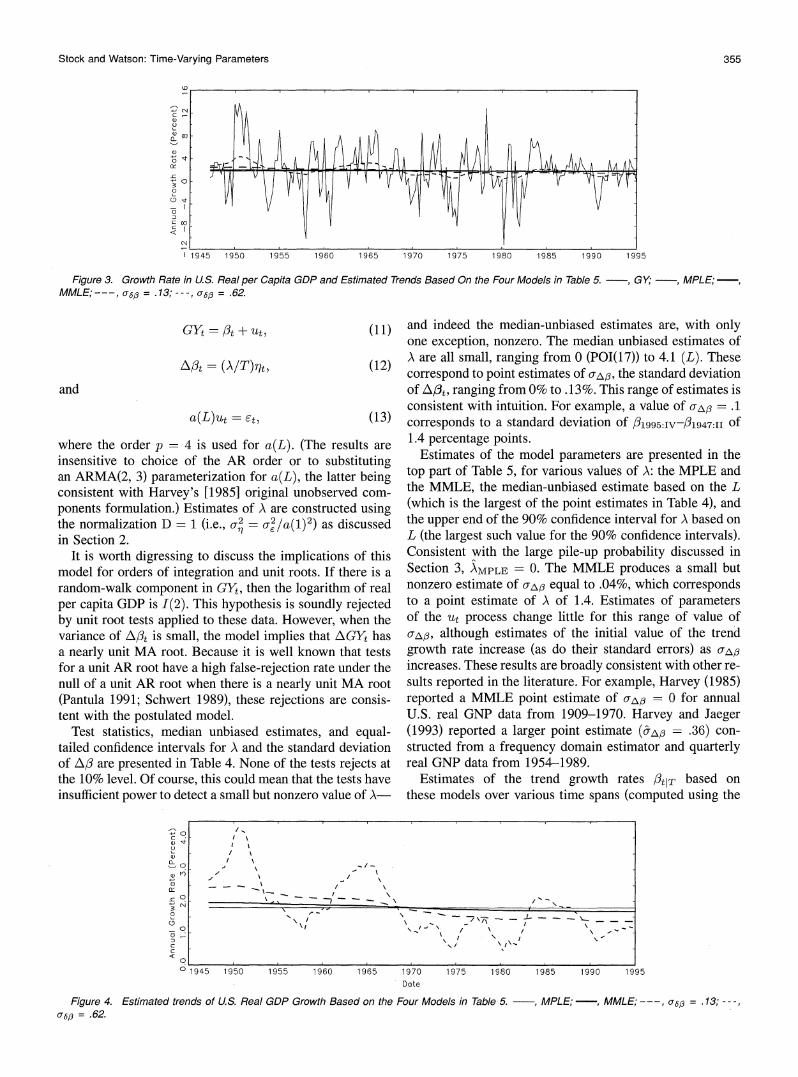
Figure 3. Growth Rate in U.S. Real per Capita GDP and Estimated Trends Based On the Four Models in Table 5. , GY , MPLE;- MMLE;---, u6,8 = .13; -- -, u6, = .62.

GYt = t + Ut, 0(11)

A =t = (A/T)rt, (12)

and

a(L)ut = Et, (13)

where the order p = 4 is used for a(L). (The results are insensitive to choice of the AR order or to substituting an ARMA(2, 3) parameterization for a(L), the latter being consistent with Harvey's [1985] original unobserved components formulation.) Estimates of A are constructed using the normalization D = 1 (i.e., ao2 - 0Q2/a(1)2) as discussed in Section 2.

It is worth digressing to discuss the implications of this model for orders of integration and unit roots. If there is a random-walk component in GYt, then the logarithm of real per capita GDP is I(2). This hypothesis is soundly rejected by unit root tests applied to these data. However, when the variance of A/t is small, the model implies that AGYt has a nearly unit MA root. Because it is well known that tests for a unit AR root have a high false-rejection rate under the null of a unit AR root when there is a nearly unit MA root (Pantula 1991; Schwert 1989), these rejections are consistent with the postulated model.

Test statistics, median unbiased estimates, and equal- tailed confidence intervals for A and the standard deviation of AO are presented in Table 4. None of the tests rejects at the 10% level. Of course, this could mean that the tests have insufficient power to detect a small but nonzero value of A-

and indeed the median-unbiased estimates are, with only one exception, nonzero. The median unbiased estimates of A are all small, ranging from 0 (POI(17)) to 4.1 (L). These correspond to point estimates of uA,, the standard deviation of A/3t, ranging from 0% to .13%. This range of estimates is consistent with intuition. For example, a value of u(, = .1 corresponds to a standard deviation of /31995:IV-31947:II of 1.4 percentage points.

Estimates of the model parameters are presented in the top part of Table 5, for various values of A: the MPLE and the MMLE, the median-unbiased estimate based on the L (which is the largest of the point estimates in Table 4), and the upper end of the 90% confidence interval for A based on L (the largest such value for the 90% confidence intervals). Consistent with the large pile-up probability discussed in Section 3, AMPLE = 0. The MMLE produces a small but nonzero estimate of uA, equal to .04%, which corresponds to a point estimate of A of 1.4. Estimates of parameters of the ut process change little for this range of value of uAo, although estimates of the initial value of the trend growth rate increase (as do their standard errors) as uA, increases. These results are broadly consistent with other results reported in the literature. For example, Harvey (1985) reported a MMLE point estimate of uA, = 0 for annual U.S. real GNP data from 1909-1970. Harvey and Jaeger (1993) reported a larger point estimate (&Afl = .36) constructed from a frequency domain estimator and quarterly real GNP data from 1954-1989.

Estimates of the trend growth rates /tIT based on these models over various time spans (computed using the

n0?

(U9 \\/- =

-;

-

<0

o 1945 1950 1955 1960 1965 1970 1975 1980 1985 1990 1995 Date

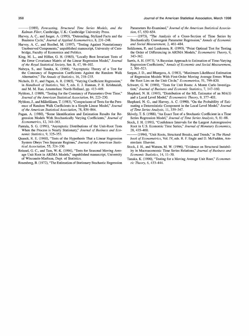
Figure 4. Estimated trends of US. Real GDP Growth Based on the Four Models in Table 5. MPLE; - , MMLE; -- = .1 3; - -, u6, = .62.


Kalman smoother) are given in the bottom part of Table 5, and these series are plotted in Figures 3 and 4. Figure 3 includes the raw data (GYt); this series is omitted from Figure 4, in which the scale is enlarged. No large mean shift is evident in the raw data, consistent with the small estimates of uA, found using the various methods. The estimate of trend per capita GDP growth based on the MPLE is, of course, a horizontal line showing the mean of the raw data. In contrast, the other estimates reflect, to a varying degree, a slowdown in mean GDP growth over this period. The point estimate based on L implies a slowdown in the annual trend growth rate of approximately .9% per annum from the 1950s to the 1990s. Finally, none of the methods detects any substantial increase in trend GDP growth over the 1990s relative to the 1980s; indeed, all of the point estimates suggest a modest decrease.

5. DISCUSSION AND CONCLUSIONS

The median unbiased estimators developed here provide empirical researchers with a device to circumvent the undesirable pile-up problem and bias of the MLE in the TVP model when coefficient variation is small. The LT- and FT-based test statistics are easily computed using statistics from the GLS regression of yt on Xt. Given these statistics, the median unbiased estimator can be obtained by interpolating the entries in a lookup table. Such a lookup table is provided here for the univariate local levels model (Table 3), and lookup tables in higher dimensions for the normalization D = Ik are available from the authors on request.

In the special case of the univariate local-level model, we examined six asymptotically median unbiased estimators and two MLEs and found considerable differences among them. The MLEs were badly biased, particularly the MPLE. When the variance of the coefficients is small, the median unbiased estimators based on the QLR and P01(17) test statistics had good AREs. Because no asymptotic theory for the POI tests in the TVP model appears to be available outside the case Xt = 1, and because the POI tests are somewhat cumbersome to compute even in the local-level model, these results provide support for using the QLR-based median unbiased estimators in the general TVP model when the coefficient instability is small.

APPENDIX: PROOF OF THEOREM 1

Before proving Theorem 1, we state and prove two prelim- inary lemmas. Let UttI - i.t_p)', A = (-ai, -a2,..., -ap)', and A (Ut1U1<1(U' 1fi) using the usual matrix notation.

Lemma A]. Under assumptions A-C, T1/2 (A - A) = Op(1).

Proof. The result follows by showing T1 /2 (A-A) ?P 0, where A = (Ut1 U_i)-1(Ut1 u), where Ut-I = (ut-i, ... . ut-PY . After straightforward algebra, it is seen that this follows if

p -LIT P 0 and /12T -P* 0, where tIlT and tt2T are matrices with (i,j) elements, it,i - T-12 Zt=1 U ( - ) and /12t,ij =T-112 ZtI1 (f3-i-' -it_( _-3). These limits follow using the Markov and Chebyschev inequalities and ap- plying assumptions A-C, assuming that T112 (p3- i3) => Op (1).

An Op (1) limiting representation for T112 ( _- 30) can be obtained using the methods in the proof of Theorem 1, but showing the T112 rate (which is all that is required here) can be verified directly using Chebyschevs' inequality.

Lemma A2. Let Zt be a mean 0 stationary vector stochastic process with fourth-order cumulants that satisfy E? rl ,r2 ,r3= oo0

IC(rl, r2, r3)1 < oo. Let wt be either a scalar nonrandom se- quence or a random variable that is independent of Zt for which supi supt>1 EIzit I4 < oo and supt>I EIwt 14 < oo. Then T-1 EZT71 ztwt p 0 uniformly in s.

Proof First let Zt be a scalar. For 3 > 0,

[Ts9] / r 4

Pr sup T-1 ZtWt > 6 < 6-4E max T-1 ztwt

T r 4\

< 6-4 E T-1 Eztwt ( r=l t=l

r 4

< -4T+-3 max E tttj l<r<T = J

T

< 6-4T-3 supEIwt {T ZE(ztr1rr) tI,t2 ,t3 ,t4= j

T

Proof~~~~~~~~~~~~t of: Thoe 1

An implication of assumptions A, B, and C, or alternatively of~~~~~r o

< a -4Tp-3isup EAwt 14 is tha t , t3t1

t~~~~~~~~U

tI ,t2,t3,t=-I

T~~~~ 2)

3T2 3 IC(tY) I 1

_ =00

We frsthe sproElwthe t assumptions,A, Br , andvC.

by Zit~~~~~

Proof of Paertm a

Lne imp l (atL)d assumptions, A, final and i vrn, srovith

asuniomptionsistency D,his etensthatottb epaigz

t=l t=

Brownianimotion o ss. pin ,B n ratraieyo Wefrtpoetetermudrassumptions A,B and DC. ta

Proof ~~~ ofPr

wheet W,= (L and W2 =Ej= areineenet_ k-imni_onal sthandr


yt =/36Xt + (Z=l Vr)'Xt + ?t + ?tt Accordingly,

CT (S) = 1T (S) + A\6T (S) + 3T (S)

- fKT(S)1{1T(1) + /A2T(1) + 63T(1)}, (A.2)

where [Ts]

1T (S) = T-1 /2 ZitfLt, t=l

[Ts] t

42(S= T / tt Vr

t=l r=l

[Ts]

3T (S) = T-1 /2 : xt(t t=l

and - [Ts] - T _-

fKT (S) = T-1 E Z T I ' ic

Limits are obtained for these terms in turn. All limits are uniform in s E [0,1].

1. Write (1T(S) AlT(S) + A2T(s) + ( T(s), where AlT(s) - j= o &i >7/ T2 (a, - ai)(T1 >s? xt-j)t-i))

A2T(S) = T1/2 Et= 1(it - Xt and -lT(1) = T1/2 ZI11 Xt?t. Assumptions A, B, and C imply that T-1 E>Ts] Xt_jut_i satisfies the conditions of Lemma A.2 with zt = Xt-jut-i and wt - 1; so, because p is fixed, AlT P 0. By an analogous argument, A2T P 0. Using the limit in (A.1), we have (IT(S) =X U,rl /2 W (S).

2. Write 42T(S) A3T(S) + A4T(S) + (2T (S), where *~~~~-/ E[Ts] 1XXi-/

A3T(S) T >tk (XtXt - r) Et=1 V, A4T(S) - T

Zt= (XtXt - XtXtk) Et r, and 42T(s) = Ts 3/2 >7"1 Er= IZJ,r To show A3T P 0 and A4T P 0, consider for nota- tional simplicity the case k = 1. (The argument for k > 1 is similar.) Note that T2 maxt1...t4 E j Zr-= vr1 r4Z = lVr4j r

supSI...s4 EjW2(si) ... W2(s4)jfQ2 < oo. Because Xt is station-

ary with absolutely summable eighth-order cumulants, Xt2-r is stationary with absolutely summable fourth-order cumulants. Thus A3T satisfies the conditions of Lemma A.2 with Zt

t - r and wt = T-12 r 1 Vr, SO A3T P 0. Turning to A4T, A4T =~0 = E 70 (&i +ai)T / (j -aj)A4T,ij(S), where

A4T,ij(S) [T-3/2 E[Ts] Xt_j Xt_jT-1/2 =3 I vr]. An argument analogous to that used for A3T shows that A4T,ij P 0 and, because p is finite, A4T -P 0. The limit of $ijT follows from (A.1). Thus 42T (s) => rPl /2 f0o W2 (r) dr.

3. Write 43T(S) = -AZEP=0 i=o j ( s3T,ilJ(S), where

63T,i1j(s) (T-3/2 E[Ts] Xt_iX/_jVt_i) As before, consider the case k 1. Now, T1/2 3T,i1j(s) satisfies Lemma A.2 with Zt Xt0X- 3_jvt-i and wt = 1; thus 63T - 0.

4. Let AlT(s) = T1 X71] (XtXt - XtXt/) and A,T(s) =

T-1 >3Ts](X)tX)t - F), and let A7T Al^T ? AlT =

T-1 >3TS7] (X0X - F). The argument that AlT P~ 0 follows the argument that A4T P~ 0 with T-~12 >3r=l Vr replaced by 1, and

the argument that A6T P 0 follows the argument that A3T P 0 with the same replacement. Thus A7T -A 0, SO K;T(S) - Slk.

Similar calculations imply that P 2 soV P rPo. By collect- ing terms and using (A.2), it follows that V"2- T(S) #> hx(s) - shA (1), where h, (s) = Wi (s) + ((r 1/2 n1 /2/u) f' W2 (r) dr.

Proof of Part b This follows from the continuous mapping theorem.

Proof of Part c This follows by straightforward but tedious manipulations using

the previous limiting results. Next, turn to the proof under assumptions A and D. Under as-

sumption D, a(L) = &(L) = 1, so Xt = Xt = Xt and et = Yt - ,3'Xt (where ,3 remains the OLS estimator). The proof under these conditions follows the foregoing proof but is simpler. In particular, (A.2) now holds with (lT(S) = T-1 /2 EtT=s Xtet,)42T(S)

T 3/2 TStj XtX't r 1 /r,3T(S) 0, and IKT(S) -

[T-1 E[T7s] XtX'][T-1 ET1 XtX']-1. The limit of 41T fol-

lows from (A.1). Write 42T(S) as 42T(S) = T-E '11(XtXt -

r)(T-1/2 Zt=1 vr) + rT-3/2 Z:1T'sZ Et=l r. The first term in this expression P 0 as a consequence of Lemma A.2 and the independence of {vt,t 1,.. ., T} and {Xt,t = 1,...,T}, as discussed earlier for the term A3T. The limit of the second term follows from (A. 1) and the continuous mapping theorem. The argument given earlier for $KT(s) P slk applies under these assumptions, and V -A o- 'r. This proves part (a) under assumptions A and D; the proof of parts (b) and (c) follows accordingly.

[Received August 1996. Revised June 1997.]

REFERENCES Andrews, D. W. K., Lee, I., and Ploberger, W. (1996), "Optimal Change-

point Tests for Normal Linear Regression," Journal of Econometrics, 70, 9-38.

Andrews, D. W. K., and Ploberger, W. (1994), "Optimal Tests When a Nui- sance Parameter is Present Only Under the Alternative," Econometrica, 62, 1383-1414.

Brillinger, D. R. (1981), Time Series: Data Analysis and Theory, San Fran- cisco: Holden-Day.

Chow, G. C. (1984), "Random and Changing Coefficient Models," in Hand- book of Econometrics, eds. Z. Griliches and M. D. Intrilligator, Amster- dam: North-Holland, chap. 21.

Cooley, T. F., and Prescott, E. C. (1973a), "An Adaptive Regression Model," International Economic Review, 14, 364-371.

(1973b), "Tests of an Adaptive Regression Model," Review of Eco- nomics and Statistics, 55, 248-256.

-~ (1976), "Estimation in the Presence of Stochastic Parameter Vari- ation," Econometrica, 44, 167-184.

Davis, R. A., and Dunsmuir, W. T. M. (1996), "Maximum Likelihood Es- timation for MA(1) Processes with a Root on or Near the Unit Circle," Econometric Theory, 12, 1-29.

Engle, R. F., and Watson, M. W. (1987), "The Kalman Filter Model: Appli- cations to Forecasting and Rational Expectations Models," in Advances in Econometrics: Fifth World Congress of the Econometric Society, ed. T. Bewley, Cambridge, U.K.: Cambridge University Press.

Franzini, L., and Harvey, A. C. (1983), "Testing for Deterministic Trend and Seasonal Components in Time Series Models," Biometrika, 70, 673- 682.

Hansen, B. E. (1992), "Tests for Parameter Instability in Regressions with I(1) Processes," Journal of Business and Economic Statistics, 10, 321- 336.

Harvey, A. C. (1985), "Trends and Cycles in Macroeconomic Time Series," Journal of Business and Economic Statistics, 3, 216-227.


(1989), Forecasting, Structural Time Series Models, and the Kalman Filter, Cambridge, U.K.: Cambridge University Press.

Harvey, A. C., and Jaeger, A. (1993), "Detrending, Stylized Facts and the Business Cycle," Journal of Applied Econometrics, 8, 231-248.

Harvey, A. C., and Streibel, M. (1997), "Testing Against Nonstationary Unobserved Components," unpublished manuscript, University of Cam- bridge, Faculty of Economics and Politics.

King, M. L., and Hillier, G. H. (1985), "Locally Best Invariant Tests of the Error Covariance Matrix of the Linear Regression Model," Journal of the Royal Statistical Society, Ser. B, 47, 98-102.

Nabeya, S., and Tanaka, K. (1988), "Asymptotic Theory of a Test for the Constancy of Regression Coefficients Against the Random Walk Alternative," The Annals of Statistics, 16, 218-235.

Nichols, D. F., and Pagan, A. R. (1985), "Varying Coefficient Regression," in Handbook of Statistics, Vol. 5, eds. E. J. Hannan, P. R. Krishnaiah, and M. M. Rao, Amsterdam: North-Holland, pp. 413-449.

Nyblom, J. (1989), "Testing for the Constancy of Parameters Over Time," Journal of the American Statistical Association, 84, 223-230.

Nyblom, J., and Makelainen, T. (1983), "Comparisons of Tests for the Pres- ence of Random Walk Coefficients in a Simple Linear Model," Journal of the American Statistical Association, 78, 856-864.

Pagan, A. (1980), "Some Identification and Estimation Results for Re- gression Models With Stochastically Varying Coefficients," Journal of Econometrics, 12, 341-363.

Pantula, S. G. (1991), "Asymptotic Distributions of the Unit-Root Tests When the Process is Nearly Stationary," Journal of Business and Eco- nomic Statistics, 9, 325-353.

Quandt, R. E. (1960), "Tests of the Hypothesis That a Linear Regression System Obeys Two Separate Regimes," Journal of the American Statis- tical Association, 55, 324-330.

Reinsel, G. C., and Tam, W.-K. (1996), "Tests for Seasonal Moving Aver- age Unit Root in ARIMA Models," unpublished manuscript, University of Wisconsin-Madison, Dept. of Statistics.

Rosenberg, B. (1972), "The Estimation of Stationary Stochastic Regression

Parameters Re-Examined," Journal of the American Statistical Associa- tion, 67, 650-654.

(1973), "The Analysis of a Cross-Section of Time Series by Stochastically Convergent Parameter Regression," Annals of Economic and Social Measurement, 2, 461-484.

Saikkonen, P,. and Luukonen, R. (1993), "Point Optimal Test for Testing the Order of Differencing in ARIMA Models," Econometric Theory, 9, 343-362.

Sarris, A. H. (1973), "A Bayesian Approach to Estimation of Time-Varying Regression Coefficients," Annals of Economic and Social Measurement, 2, 501-523.

Sargan, J. D., and Bhargava, A. (1983), "Maximum Likelihood Estimation of Regression Models With First-Order Moving Average Errors When the Root Lies on the Unit Circle," Econometrica, 51, 799-820.

Schwert, G. W. (1989), "Tests for Unit Roots: A Monte Carlo Investiga- tion," Journal of Business and Economic Statistics, 7, 147-160.

Shephard, N. H. (1993), "Distribution of the ML Estimator of an MA(1) and a Local Level Model," Econometric Theory, 9, 377-401.

Shephard, N. G., and Harvey, A. C. (1990), "On the Probability of Esti- mating a Deterministic Component in the Local Level Model," Journal of Time Series Analysis, 11, 339-347.

Shively, T. S. (1988), "An Exact Test of a Stochastic Coefficient in a Time Series Regression Model," Journal of Time Series Analysis, 9, 81-88.

Stock, J. H. (1991), "Confidence Intervals for the Largest Autoregressive Root in U.S. Economic Time Series," Journal of Monetary Economics, 28, 435-460.

(1994), "Unit Roots, Structural Breaks, and Trends," in The Hand- book of Econometrics, Vol. IV, eds. R. F. Engle and D. McFadden, Am- sterdam: Elsevier.

Stock, J. H., and Watson, M. W. (1996), "Evidence on Structural Instabil- ity in Macroeconomic Time Series Relations," Journal of Business and Economic Statistics, 14, 11-30.

Tanaka, K. (1990), "Testing for a Moving Average Unit Root," Economet- ric Theory, 6, 433-444.

Median Unbiased Estimation of Coefficient Variance in a Time-Varying Parameter … ·...

Documents

Transcript of Median Unbiased Estimation of Coefficient Variance in a Time-Varying Parameter … ·...