Mechanical Vibration Lab...Mechanical Vibration Lab Philadelphia Unversity Page 9 of 64 Equations of...

Philadelphia University

Faculty of Engineering

Mechanical Engineering Department

Mechanical Vibration Lab

of 64

Table of contents

No. Experiment

0 Vibration Review

1 Mass – Spring system

2 Simple and Compound Pendulums

3 Mass Moment of Inertia Estimation-Part one: Bifilar Suspension

4 Mass Moment of Inertia Estimation-Part two: Auxiliary Mass Method

5 Forced Vibration with Negligible Damping

6 Transverse Vibration of a Beam

7 Undamped vibration absorber

8 Static and Dynamic Balancing

of 64

ELEMENTARY PARTS OF VIBRATORY SYSTEMS

Vibratory systems comprise means for storing potential energy (spring), means for

storing kinetic energy (mass or inertia), and means by which the energy is gradually lost

(damper). The vibration of a system involves the alternating transfer of energy

between its potential and kinetic forms. In a damped system, some energy is dissi-

pated at each cycle of vibration and must be replaced from an external source if a

steady vibration is to be maintained. Although a single physical structure may store

both kinetic and potential energy, and may dissipate energy, this chapter considers

only lumped parameter systems composed of ideal springs, masses, and dampers

wherein each element has only a single function. In translational motion, displace-

ments are defined as linear distances; in rotational motion, displacements are

defined as angular motions.

TRANSLATIONAL MOTION

Spring:- In the linear spring shown in Figure1, the change in the length of the spring is

proportional to the force acting along its length:

F = k(x - u) (1)

The ideal spring is considered to have no mass; thus, the force acting on one end is

equal and opposite to the force acting on the other end. The constant of proportionality k

is the spring constant or stiffness.

Figure1. Linear spring.

Mass:- A mass is a rigid body (Figure 2) whose acceleration x according to Newton’s

second law is proportional to the resultant F of all forces acting on the mass:*

F = m x (2)

of 64

Figure 2. Rigid mass.

Damper. In the viscous damper shown in Figure 3, the applied force is proportional

to the relative velocity of its connection points:

F = c(x - u ) (3)

The constant c is the damping coefficient, the characteristic parameter of the damper. The

ideal damper is considered to have no mass; thus the force at one end is equal and

opposite to the force at the other end.

Figure.3 Viscous damper.

ROTATIONAL MOTION

The elements of a mechanical system which moves with pure rotation of the parts are

wholly analogous to the elements of a system that moves with pure translation. The

property of a rotational system which stores kinetic energy is inertia; stiffness and

damping coefficients are defined with reference to angular displacement and angular

velocity, respectively. The analogous quantities and equations are listed in Table.1.

TABLE 1. Analogous Quantities in Translational and Rotational Vibrating Systems

Translational quentity rototinal quantity

Linear displacement x Angular displacement Force F Torque M

Spring constant k Spring constant kr

Damping constant c Damping constant cr

Mass m Moment of inertia I

Spring law F k(x1 x2) Spring law M kr(1 2)

Damping law F c(x1 x2) Damping law M cr( 1 2)

Inertia law F mx Inertia law M I

In as much as the mathematical equations for a rotational system can be written by analogy

from the equations for a translational system, only the latter are discussed in detail.

Whenever translational systems are discussed, it is understood that corresponding equations

of 64

apply to the analogous rotational system, as indicated in Table.1.

PERIODIC MOTION

Vibration is a periodic motion, or one that repeats itself after a certain interval of time called the

period, T. Figure 4. illustrated the periodic motion time-domain curve of a steam turbine bearing

pedestal. Displacement is plotted on the vertical, or Y-axis, and time on the horizontal, or X-

axis. The curve shown in Figure 5 is the sum of all vibration components generated by the

rotating element and bearing-support structure

Figure 4. Periodic motion for bearing pedestal of a steam turbine.

Figure 5 Discrete (harmonic) and total (none-harmonic) time-domain vibration

curves.

of 64

˙

MEASURABLE PARAMETERS

As shown previously, vibrations can be displayed graphically as plots, which are referred

to as vibration profiles or signatures. These plots are based on measurable parameters (i.e.,

frequency and amplitude). Note that the terms profile and signature are sometimes used

interchangeably by industry. In this module, however, profile is used to refer either to time-

domain (also may be called time trace or waveform) or frequency-domain plot.

Frequency

Frequency is defined as the number of repetitions of a specific forcing function or vibration

component over a specific unit of time. Take for example a four-spoke wheel with an

accelerometer attached. Every time the shaft completes one rotation, each of the four spokes

passes the accelerometer once, which is referred to as four cycles per revolution. Therefore, if

the shaft rotates at 100 rpm, the frequency of the spokes passing the accelerometer is 400 cycles

per minute (cpm). In addition to cpm, frequency is commonly expressed in cycles per second

(cps) or Hertz (Hz).

Amplitude

Amplitude refers to the maximum value of a motion or vibration. This value can be

represented in terms of displacement (mils), velocity (inches per second), or acceleration (inches

per second squared), each of which is discussed in more detail in the following section on

Maximum Vibration Measurement.

Displacement

Displacement is the actual change in distance or position of an object relative to a reference

point and is usually expressed in units of mils, 0.001 inch. For example, displacement is the

actual radial or axial movement of the shaft in relation to the normal centerline usually using

the machine housing as the stationary reference. Vibration data, such as shaft displacement

measurements acquired using a proximity probe or displacement transducer should always be

expressed in terms of mils, peak – peak

Velocity

Velocity is defined as the time rate of change of displacement (i.e., the first derivative, 𝑑𝑋

𝑑𝑡 or ��)

and is usually expressed as inches per second (in./sec). In simple terms, velocity is a

description of how fast a vibration component is moving rather than how far, which is described

by displacement.

of 64

Acceleration

Acceleration is defined as the time rate of change of velocity (i.e., second derivative of

displacement, 𝑑2𝑋

𝑑𝑡2 or ��) is expressed in units of inches per second squared ( inch/ sec2 )

Acceleration is commonly expressed in terms of the gravitational constant, g, which is 32.17

ft/sec2. In vibration analysis applications, acceleration is typically expressed in terms of g-RMS

or g-PK. These are the best measures of the force generated by a machine, a group of

components, or one of its components.

of 64

TYPES OF VIBRATION

Vibration Classifications

Linearity

linear

non - linear

Excitation

free

force

Damping

undamped

damped

Countinuty

continous

descrite

period of ocsillation

harmonic

periodic

general

random

Mechanical Vibration Lab Philadelphia Unversity

Page 8 of 64

Newtown Laws of motion

Newton's First Law of Motion:

Every object in a state of uniform motion tends to remain in that state of motion unless an

external force is applied to it.

Newton's Second Law of Motion:

The relationship between an object's mass m, its acceleration a, and the applied force F is

F = ma. Acceleration and force are vectors; in this law the direction of the force vector is

the same as the direction of the acceleration vector.

Newton's Third Law of Motion:

For every action there is an equal and opposite reaction.

Free Body Diagrams ( F.B.D )

Drawing Free-Body Diagrams

Free-body diagrams are diagrams used to show the relative

magnitude and direction of all forces acting upon an object

in a given situation. A free-body diagram is a special

example of the vector diagrams. These diagrams will be

used throughout our study of physics. The size of the

arrow in a free-body diagram is reflects the magnitude of

the force. The direction of the arrow shows the direction

which the force is acting. Each force arrow in the diagram is labeled to indicate the exact

type of force. It is generally customary in a free-body diagram to represent the object by a

box and to draw the force arrow from the center of the box outward in the direction

which the force is acting. An example of a free-body diagram is shown at the right.

The free-body diagram above depicts four forces acting upon the object. Objects do not

necessarily always have four forces acting upon them. There will be cases in which the

number of forces depicted by a free-body diagram will be one, two, or three. There is no

hard and fast rule about the number of forces which must be drawn in a free-body

diagram. The only rule for drawing free-body diagrams is to depict all the forces which

exist for that object in the given situation. Thus, to construct free-body diagrams, it is

extremely important to know the various types of forces. If given a description of a

physical situation, begin by using your understanding of the force types to identify which

forces are present. Then determine the direction in which each force is acting. Finally,

draw a box and add arrows for each existing force in the appropriate direction; label each

force arrow according to its type. If necessary, refer to the list of forces and their

description in order to understand the various force types and their appropriate symbols.

http://www.glenbrook.k12.il.us/GBSSCI/PHYS/Class/newtlaws/u2l2b.html#Top

http://www.glenbrook.k12.il.us/GBSSCI/PHYS/Class/newtlaws/u2l2b.html#Help

http://www.glenbrook.k12.il.us/GBSSCI/PHYS/Class/newtlaws/u2l2b.html#Help


Page 9 of 64

Equations of motion:-

When a body is moving with a constant acceleration, the following relations are valid for

the distance, velocity and acceleration.

By substituting (1) into (2), we can get (3), (4) and (5)

where

s = the distance between initial and final positions (displacement) (sometimes

denoted R or x)

u = the initial velocity (speed in a given direction)

v = the final velocity

a = the constant acceleration

t = the time taken to move from the initial state to the final state


Page 10 of 64

Report writing

Every student is required to submit his own separate report for each test

conducted. Reports should be in hand-writing, on A4 paper. In general, the

reports should be arranged in the following order:

1- Abstract

(An abstract is a self-contained, short, and powerful statement that describes a

larger work. Components vary according to discipline. An abstract of a social

science or scientific work may contain the scope, purpose, results, and contents of

the work.)

2- Introduction

(Begin with background knowledge-What was known before the lab? What is the

lab about? Include any preliminary/pre-lab questions. Also, include the purpose of

the lab at the end of the introduction. Be clear & concise)

3- Materials and Equipment

(Can usually be a simple list, but make sure it is accurate and complete.)

4- Procedure

(Describe what was performed during the lab Using clear paragraph structure,

explain all steps in the order they actually happened, If procedure is taken directly

from the lab handout, say so! Do NOT rewrite the procedure!)

5- Collected Data

(Label clearly what was measured or observed throughout the lab Include all data

tables and/or observation)


Page 11 of 64

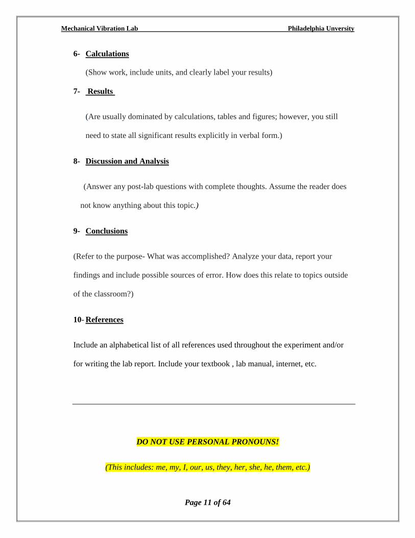
6- Calculations

(Show work, include units, and clearly label your results)

7- Results

(Are usually dominated by calculations, tables and figures; however, you still

need to state all significant results explicitly in verbal form.)

8- Discussion and Analysis

(Answer any post-lab questions with complete thoughts. Assume the reader does

not know anything about this topic.)

9- Conclusions

(Refer to the purpose- What was accomplished? Analyze your data, report your

findings and include possible sources of error. How does this relate to topics outside

of the classroom?)

10- References

Include an alphabetical list of all references used throughout the experiment and/or

for writing the lab report. Include your textbook , lab manual, internet, etc.

DO NOT USE PERSONAL PRONOUNS!

(This includes: me, my, I, our, us, they, her, she, he, them, etc.)


Page 12 of 64

I- Objectives:

1) To determine the stiffness of a helical spring using two methods;

a -Deflection curve and Hook’s Law.

b -Time measurements.

Then to compare their results with the analytical value.

2) To find the effective mass of the spring that has been used.

3) To evaluate the gravitational acceleration constant g.

4) To estimate the value of the modulus of rigidity G for the material of the helical

spring, and compare it with the standard value for steel.

II- System Description:

The spring-mass system in Figure1.1 shows an extension linear helical spring with an

initial free length Li, effective mass mS, supported vertically from one of its ends; while

the other end is free to elongate and attached to a load-carrier of mass. The free length of

the spring loaded with the load carrier alone is Lo. Disks each of (md = 0.4 kg) mass are

added to the carrier gradually, and each loading state causes the spring to elongate by the

distance from its unloaded length Lo to get a total length of L.

Lo

L

Disk

md

Load-Carrier

mc

Y

Spring

ms

Figure 1.1 General layout of the experiment set-up


Page 13 of 64

III- Governing Equations:

For the spring-mass system shown in Figure-1.1, in the case of free vibration in the

vertical direction Y, the equation of motion of the system is given by:

M�� + Ky=0 (1)

where:

M is the total mass of the system, and equals to: SC mmmM

m is the total mass of the disks: dmm ∑

From the equation of motion, we can find that:

* Natural frequency=M

Kn (2)

* Period of oscillation=K

mmm2

K

M2

2 SC

n

(3)

For the linear spring following Hook’s law, then:

KFS (4)

But for the present system, the spring force FS is also given by:

mgFS (5)

Combine eqns-4 & 5, to get:

g

Km (6)

For a helical spring, the stiffness is expressed analytically as:

3

4

ND8

GdK (7)


Page 14 of 64

IV- Experimental Procedures:

1. Hang the spring vertically with the load carrier attached to its end, and then

measure the total length of the spring Lo. (This length is not the initial free length

of the spring Li )

2. Add one disk to the carrier (m = md), and measure the total length of the spring

after elongation L.

3. With this loading, stretch the spring downward, then leave it to oscillate freely

and record the time needed to complete ten oscillations T.

4. Add another disk so that (m = 2md), and repeat steps-2 & 3.

5. Continue by adding a disk each time for total ten disks (m = 10md), and each

time measure the parameters L and T.

V- Collected Data:

Table-1.1 Data collected from the experiment execution

Trial m (kg) L (cm) T (second)

1

2

3

4

5

6

7

8

9

10

Table-1.2 Dimensions and parameters of the spring

Parameter Value

N (turns)

D (mm)

d (mm)

Lo (cm)


Page 15 of 64

VI- Data Processing:

Square eqn-3, to get: SC

22 mmm

K

4

Draw 2 versus m ( call it figure 1.2 )

1. Slope K

4S

2

1

K is determined.

2. Intercept with the vertical axis SC

2

Inter mmK

4Y

mS is determined.

3. Intercept with the horizontal axis SCInter mmX - mS is verified.

From eqn-6: g

Km

Draw m versus ( call it figure 1.3 )

1. Slope g

KS2 K is also obtained.

2. Multiply the slopes of the previous two steps. You get the value: g

4SS

2

21

g

is found, and compared to the standard value.

Use eqn-7: 3

4

ND8

GdK

1. Find K directly.

2. Compare the two experimental values of K obtained before, with this theoretical

value.


Page 16 of 64

VII- Results:

Table-1.3 Data processing analysis

Trial m (kg) (mm) (second) 2 (second)

2

1

2

3

4

5

6

7

8

9

10

Table-1.4 Data processing results

Spring Stiffness K

K (theoretical) = …………… (N/m)

From: Slope K (N/m) Percent Error ()

Figure-1.2

Figure-1.3

Spring Effective Mass ms

From Figure-1.2:

YInter (kg.m/N) ms (kg)

XInter (kg) ms (kg)

Gravitational Acceleration g

From Figures-

1.2 & 1.3

S1S2 (sec2/m) g (m/sec

2) Percent Error ()

modulus of rigidity G

From Figures-

1.2

slope (m/N) G (Gpa) Percent Error ()


Page 17 of 64

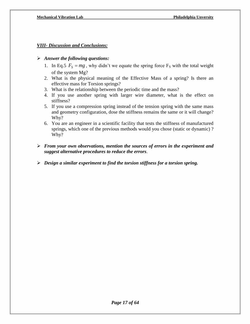
VIII- Discussion and Conclusions:

Answer the following questions:

1. In Eq.5 mgFS , why didn’t we equate the spring force FS with the total weight

of the system Mg?

2. What is the physical meaning of the Effective Mass of a spring? Is there an

effective mass for Torsion springs?

3. What is the relationship between the periodic time and the mass?

4. If you use another spring with larger wire diameter, what is the effect on

stiffness?

5. If you use a compression spring instead of the tension spring with the same mass

and geometry configuration, dose the stiffness remains the same or it will change?

Why?

6. You are an engineer in a scientific facility that tests the stiffness of manufactured

springs, which one of the previous methods would you chose (static or dynamic) ?

Why?

From your own observations, mention the sources of errors in the experiment and

suggest alternative procedures to reduce the errors.

Design a similar experiment to find the torsion stiffness for a torsion spring.


Page 18 of 64

I- Introduction:

Simple pendulum is simply a concentrated mass m attached to one of the ends of a

mass-less cord of length l, while the other end is fitted as a point of oscillation, such that

the mass is free to oscillate about that fixed point in the vertical plane. The compound

pendulum differs from the simple one in that it has a mass distribution along its length -

that is its mass is not concentrated at a given point-, therefore it has a mass moment of

inertia I about its mass centre.

Any rigid body that has a mass m, and mass moment of inertia I and suspended at a given

distance h from its centre of gravity represents a compound pendulum.

It should be realised in the derivation of the governing equations, that the angle of

oscillation of the pendulum, simple or compound, should be small.

II- Objectives:

This experiment aims at studying the behaviour of both simple and compound

pendulums, in order to realise the following objectives:

1. The independence of the period of oscillation of the simple pendulum from its

mass.

2. The relationship between the period of oscillation and its length.

3. The determination of the value of the gravitational acceleration g, to be compared

with the known standard value.

4. Find the radius of gyration for a compound pendulum

III- System Description:

Part One- Simple Pendulum:

The schematic representation of the simple pendulum is shown in Figure-2.1-a,

which consists of a small ball of mass m suspended by a mass-less cord of length l. The

system is given an initial small angular displacement , and as a result the pendulum

oscillates in the vertical plane by a time varying angle (t) with the vertical direction.

Part Two- Compound Pendulum:

The compound pendulum is schematically shown in Figure-2.2-b below, and it

consists of a uniform slender bar of total mass m and length l, which may be suspended at


Page 19 of 64

various points A along the bar with the aid of a sliding pivot situated at any distance h

from the centre of gravity of the pendulum.

(For this case, the centre of mass is at the middle of the rod).

As a result of an initial angular displacement the pendulum oscillates also with a

time-varying angle (t) with the vertical direction.

Figure-2.1 Schematic representation of the (a)simple pendulum (b)compound pendulum

IV- Governing Equations:

Part One - Simple Pendulum:

The dynamic equilibrium equation (equation of motion) corresponding to the

tangential direction of motion of the concentrated mass yields:

mI��+ mgsin 𝜃 = 0 (1)

Assuming small magnitude for the angle , so that sin , and simplifying eqn-1

leads to the equation:

��+ 𝑔

𝐼 𝜃= 0 (2)

l

m

l/2

hRod

(l,m)

A

neutral

positionneutral

position

Centre of

Gravity CG

(a)

Simple Pendulum

(b)

Compound Pendulum

A


Page 20 of 64

Let the motion defined by the function (t) be a simple harmonic motion defined

as 𝛉(𝐭) = 𝛂𝐬𝐢𝐧n t , where n is the natural frequency of the pendulum. Substituting for

in eqn-2 and simplifying gives n as:

l

gn (3)

The period of oscillation , is defined as the time required to complete one full cycle of

motion or one oscillation. By observing the function (t), the period is given as:

g

l2

2

n

(4)


For the compound pendulum, the dynamic equilibrium equation is obtained by

taking the moments about pivot point A as given below:

IA ��+ mgsin𝜃 =0 (5)

where; IA is the mass moment of inertia of the rod about the pivot point A.

Assuming small angle of oscillation and simple harmonic motion for (t), leads to the

following expressions for the natural frequency n and period , respectively:

A

nI

mgh=ω (6)

mgh

I Aπ2τ= (7)

The mass moment of inertia about the pivot point IA, is defined in terms of the mass

moment of inertia about the centre of gravity ICG and the distance h between the centre of

gravity and the pivot point A as: 2mhII CGA += (8)

or

)hK(mI 22CGA (9)

where; KCG is the radius of gyration of the rod about the centre of gravity.


Page 21 of 64

Using eqns-7 & 9, then the period of oscillation of the compound pendulum is given

by the expression:

gh

hK2

22GC

(10)

V- Experimental Procedures:


Steel and plastic balls are used separately in this experiment as follows:

1. Attach the cord to the steel ball at one end, and attach the other end to the main frame.

Record the length of the cord l.

2. Displace the ball form its neutral position by a small amount, and then release it to

oscillate freely. Measure and record the time T required to complete ten oscillations.

3. Adjust the cord length to a new value and repeat step-2.

4. Repeat Step-3 six more times so that eight pairs of l and T are recorded.

5. Replace the steel ball with the plastic ball and repeat steps-1 through 4.


The experimental procedures for the compound pendulum part are carried out

through the following steps:

1. Measure and record the total length l of the rod. Since the rod is uniform, the

geometrical centre point coincides with the rod's centre of gravity CG.

2. Pivot the rod at an arbitrary point A, and measure the distance from that point to the

centre of gravity h. Displace the rod by a small angle from its neutral position and

release it freely, then measure and record the time required to complete ten

oscillations T.

3. Change the pivoting point A and repeat step-2.

4. Repeat step-3 eight more times so that ten pairs of h and T are recorded.


Page 22 of 64

VI- Collected Data:


Table-2.1 Collected data for the simple pendulum part


l = …………cm

Table-2.2 Collected data for the compound pendulum part

Trial h (cm) T (second)

1

2

3

4

5

6

7

8

9

10

Trial Steel Ball Plastic Ball

l (cm) T (second) l (cm) T (second)

1

2

3

4

5

6

7

8

9

10


Page 23 of 64

VII- Data Processing:


Use eqn-4: g

l2

Evaluate the theoretical period Theor corresponding to each length l.

The values of Theor are to be compared with the experimental values Exper.

Square both sides of eqn-4 to get: g

lπτ 22 4

Draw 2 versus l ( call it Figure 2.2)

Slope = g

24 g is found and compared to the standard value.


Square eqn-10 and rearrange to get: 22CG

22 hK

g

4h

Draw 2h versus h

2 ( call it Figure-2.3)

1. Slope = g

4 2 find g and compare it to the standard value.

2. Intercept with the vertical axis 2

24CGInt K

gY

KCG is obtained.

3. Intercept with the horizontal axis 2CGInt KX KCG is verified.

Draw versus h ( call it Figure-2.4.)

Find min and the corresponding value of h.


Page 24 of 64

VIII- Results:


Table-2.3 Data processing analysis for the simple pendulum part

Steel Ball

Trial l

(cm)

Exper

(second)

Theor

(second)

(Exper.)2

(second)2

Percent

Error ()

1

2

3

4

5

6

7

8

9

10

Table-2.4 Data processing analysis for the simple pendulum part

Plastic Ball

Trial l

(cm)

Exper

(second)

Theor

(second)

(Exper.)2

(second)2

Percent

Error ()

1

2

3

4

5

6

7

8

9

10


Page 25 of 64

Table-2.5 Data processing results for the simple pendulum part.

Quantity Slope from

Figure-2.2:

g (m/s2) Percentage Error

of g ()

Steel Ball

Plastic Ball


Table-2.6 Data processing analysis for the compound pendulum part.

Trial h (cm) (second) h2 (cm)

2

2h (cm.sec

2)

1

2

3

4

5

6

7

8

9

10

Table-2.7 Data processing results for the compound pendulum part

From Figure-2.3

Slope (sec.2/m) g (m

2/sec.) Percent Error ()

YInt (sec2.m) KCG (cm)

XInt (m2) KCG (cm) Percent Error ()

From Figure-2.4

min (sec.)

h at = min (cm)


Page 26 of 64

IX- Discussion And Conclusions:

Answer the follwing questions:-

1. What do we mean by “Simple Harmonic Motion” (SHM)?

2. Why did we use two masses with identical geometries for the simple pendulum

experiment?

3. What is the physical meaning of h being equal to zero? What is the

corresponding period of oscillation?

4. Why does the compound pendulum have the identity of possessing two values of

h corresponding to the same period of oscillation ?

5. Based on the equation of motion, what is the difference between the simple and

compound pendulums? How can we replace the compound pendulum with a

simple pendulum having the same period of oscillation?



Mention some applications of both simple and compound pendelums in practical

life.

Discuss the physical meaning of the radius of gyration and give examples for it is

importance from practical life.

In this experimet, we use pendelums to find the gravitional accelertaion. Design

another experiment with different proceduers for the same perpouce.


Page 27 of 64

I- Introduction:

The Bifilar Suspension is a technique that could be applied to objects of different

shapes, but capable to be suspended by two parallel equal-length cables, in order to

evaluate its mass moment of inertia I about any point within the body.

In this experiment, the technique will be applied to find the mass moment of inertia of a

regular cross-section steel beam about its centre of gravity.

II- Objectives:

This experiment is to be performed in order to evaluate the mass moment of inertia

of a prismatic beam by introducing the method of Bifilar Suspension Technique.


The layout of the experiment is shown schematically in Figure-3.1, in which we

have a regular rectangular cross-section steel beam, of length L, total mass M, and mass

moment of inertia about its centre of gravity I. The beam is suspended horizontally

through two vertical chords, each of length l, and at distance b/2 from the middle of the

beam CG.(Two small chucks are provided for attachment).

The system is initially balanced, and by exerting a small pulse in such a way that the

beam keeps oscillating in the horizontal plane about its middle point (centre of gravity

CG), then by virtue of the tension forces initiated in the suspension chords, the beam will

oscillate making an angle θ with its neutral axis, and the suspension chords will make an

angle with the original vertical position.

Figure-3.1 General layout of the Bifilar Suspension


Page 28 of 64


In the system shown in Figure-3.1, and under equilibrium conditions, the tension

force in each chord is equal to Mg/2, and by disturbing the system with an initial angular

displacement about the middle point in the horizontal plane, it will oscillate with a

time-varying angle θ(t) under the action of the tension forces in the chords.

Taking the summation of moments about the middle point (Centre of Gravity CG), we

get the equation of motion as:

I��+(Mgb

2 ) ∅ = 0 (1)

But:

lb

2

(By equating the length of the arc of oscillation)

Substituting in eqn-1, and rearranging:

�� + (𝑀𝑔𝑏2

4𝐼𝑙) 𝜃 = 0 (2)

From the above equation of motion, we find that:

* Natural frequency = Il

Mgbn

4

2

(3)

* Period of oscillation = 2

42

2

Mgb

Il

n

(4)

# Analytical Solution:

Using the dimensions of the beam, then its mass moment of inertia about the centre

of gravity can be found analytically as follows:

I = I (solid beam) – I (holes) + I (two chucks) = IS – IH + IC (5)

12

whL

12

LMI

32S

S

(6)

2222

H2

HH X2r2

15hrXM2rM

2

15I ∑∑ (7)


Page 29 of 64

2

brhr

2

bM2rMI

22

CC2

C

2

C2

CCC

(8)

Where:-

r: the radius of each hole.

X: the distance between the hole and the middle point of the beam.

rC: the radius of the chuck.

hC: the height of the chuck.

The geometry and the definitions of the basic parameters of the system are provided in

Figure-3.1.


1- Attach the first chord to the main frame and measure its length, then attach the second

chord to the main frame with the same length as the first one. (The length to be

measured and included in the calculations l should include both the chord’s length

and the chuck’s height, see Figure-3.1)

2- Insert a slender rod through the middle hole of the beam, to provide as an axis of

rotation for the beam.

3- Hold the slender rod in place and give the beam a small displacement from one of its

ends in the transverse direction. The beam should oscillate in the horizontal plane

only.

4- Measure the time elapsed to complete ten oscillations T.

5- Release the chords then re-attach them at another length l, and repeat steps-2, 3 & 4.

6- Repeat step-5 four more times to get total six pairs of l and T.

VI- Collected Data:

Basic Parameters:

Table-3.1 Dimensions to be used according to Figure-3.1

Parameter Value Parameter Value

L (cm) rc (mm)

w (mm) hc (mm)

h (mm) R (mm)

b (mm) hm (mm)

r (mm)


Page 30 of 64

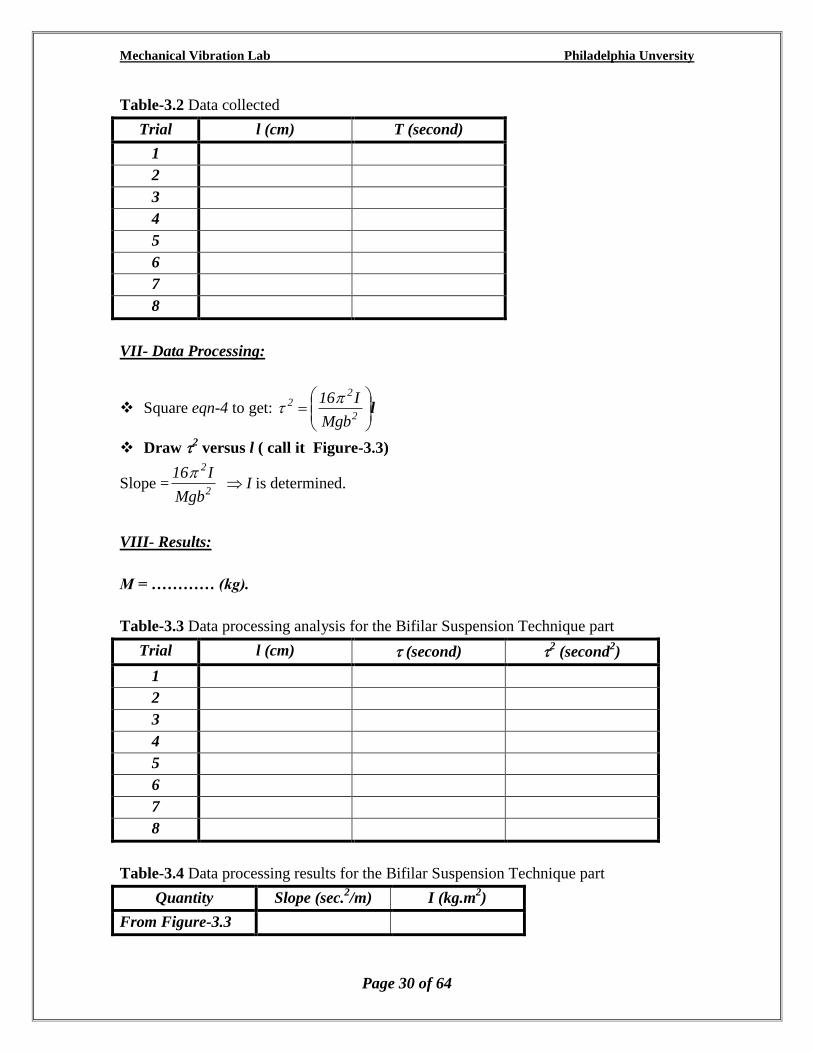
Table-3.2 Data collected

Trial l (cm) T (second)

1

2

3

4

5

6

7

8


Square eqn-4 to get: l

2

22

Mgb

I16

Draw 2 versus l ( call it Figure-3.3)

Slope =2

2

Mgb

I16 I is determined.

VIII- Results:

M = ………… (kg).

Table-3.3 Data processing analysis for the Bifilar Suspension Technique part

Trial l (cm) (second) 2 (second

2)

1

2

3

4

5

6

7

8

Table-3.4 Data processing results for the Bifilar Suspension Technique part

Quantity Slope (sec.2/m) I (kg.m

2)

From Figure-3.3


Page 31 of 64

Analytical Solution:

Table-3.5 Analytical determination of the mass moment of inertia I

IS (kg.m2)

IH (kg.m2)

IC (kg.m2)

I =IS IH + IC (kg.m2)


Answer the follwoing questions:-

1- In the first part, what modifications should be done (concerning the derivation of

equation of motion) in order to determine the mass moment of inertia about any

point other than the middle point of the beam? Derive the equation of motion for

this case.

2- Referring to the derivation of the equation of motion for the beam, why is it

important to keep the angle of oscillation of the beam small during the execution

of the experiment? What is the basic assumption that is based on assuming a small

angle of oscillation?



Design other procedures to find the mass moment of inertia other than the used in

this experiment.


Page 32 of 64

I- Introduction:

In this experiment, the two identical masses will be added to the primary system

discussed in the previous experiment to find the mass moment of inertia of a regular

cross-section steel beam about its centre of gravity.

II- Objectives:

This experiment is to be performed in order to evaluate the mass moment of inertia

of a prismatic beam by introducing the method the Auxiliary Mass.

Then the values obtained from the this method will be compared with the values obtained

experimentally and analytically in the previous experiment.


The layout of the experiment is shown schematically in Figure-4.1, in which we

have a regular rectangular cross-section steel beam, of length L, total mass M, and mass

moment of inertia about its centre of gravity I. The beam is suspended horizontally

through two vertical chords, each of length l, and at distance b/2 from the middle of the

beam CG.(Two small chucks are provided for attachment).

The system is initially balanced, and by exerting a small pulse in such a way that the

beam keeps oscillating in the horizontal plane about its middle point (centre of gravity

CG), then by virtue of the tension forces initiated in the suspension chords, the beam will

oscillate making an angle θ with its neutral axis, and the suspension chords will make an

angle with the original vertical position.


Page 33 of 64

Figure-4.1 General layout of the Bifilar Suspension


Consider the previous system with the addition of two identical circular disks of

radius R, mass m, and inertia Im; each at a side at distance Y from the middle of the beam.

The resulting equation of motion of the modified system will be:

( I + 2Im) �� + ((𝑀+2𝑚)𝑔 𝑏2

4𝑙) 𝜃 =0 (1)

Where:-

Im = m ( 𝑅2 + 𝑌2), m2hRm

Rearrange eqn-1, yields:

�� + ((𝑀+2𝑚)𝑔 𝑏2

4𝑙(𝐼+𝐼𝑚)) 𝜃 =0 (2)

From eqn-2, the natural frequency and the period of oscillation are found as:


Page 34 of 64

* Natural frequency = m

nIIl

mMgb

24

22

(3)

* Period of oscillation = mMgb

IIl m

n 2

242

22

(4)


Using the dimensions of the beam, then its mass moment of inertia about the centre

of gravity can be found analytically as follows:

I = I (solid beam) – I (holes) + I (two chucks) = IS – IH + IC (5)

12

whL

12

LMI

32S

S

(6)

2222

H2

HH X2r2

15hrXM2rM

2

15I ∑∑ (7)

2

brhr

2

bM2rMI

22

CC2

C

2

C2

CCC

(8)

Where:-

r: the radius of each hole.

X: the distance between the hole and the middle point of the beam.

rC: the radius of the chuck.

hC: the height of the chuck.

The geometry and the definitions of the basic parameters of the system are provided in

Figure-4.1.


1- Fix the examined system at any length l.

2- Put the two disks (auxiliary masses) at distance Y from the beam’s middle point, each

at a side, and record the value of Y.

3- Displace the beam slightly as in the previous part, and again measure the time elapsed

in ten oscillations T.

4- Change the positions of the two masses to new value of Y, then repeat step-3.

5- Repeat step-4 for total different six values of Y.

VI- Collected Data:


Page 35 of 64

Basic Parameters:

Table-4.1 Dimensions to be used according to Figure-4.1


L (cm) rc (mm)

w (mm) hc (mm)

h (mm) R (mm)

b (mm) hm (mm)

r (mm)

l = ……………(cm)

m = ……………(kg)

Table-4.2 Data collected for the Auxiliary Mass Method part

Trial Y (cm) T (second)

1

2

3

4

5

6


Square eqn-8 to get: mMgb

IIl m

2

2162

2

2

Draw 2 versus Im ( call I Figure-4.4)

1- Slope = mMgb

l

2

322

2

Determine g and compare it with the standard value.

2- Interception with the vertical axis mMgb

IlYInt

2

162

2

I is determined.

3- Interception with the horizontal axis 2

IX Int I is verified.

VIII- Results:


Page 36 of 64

Table-4.3 Data processing analysis for the Auxiliary Mass Method part

Trial Y (cm) Im (kg.m2) 2

(second2)

1

2

3

4

5

6

Table-4.4 Data processing results for the Auxiliary Mass Method part

From Figure-4.4

Slope (s2/m

2.kg) g (m/sec.

2)

YInt (sec.2) I (kg.m

2)

XInt (kg.m2) I (kg.m

2)


Table-4.5 Analytical determination of the mass moment of inertia I

IS (kg.m2)

IH (kg.m2)

IC (kg.m2)

I =IS IH + IC (kg.m2)

Comparison:

Table-4.6 Comparison of I obtained by the two methods with the analytical value

Method: I (kg.m2) Percentage Error ()

Analytically

Bifilar Suspension

Auxiliary Mass(Xint)

Auxiliary Mass(Yint)



Page 37 of 64

Answer the follwoing questions:-

1. In the second part (the Auxiliary Mass Method part), is it acceptable to use only

one mass at either sides of the beam? Explain?



Design other procedures to find the mass moment of inertia other than the used in

this experiment.


Page 38 of 64

I- Introduction:

Forced Vibrations is that mode of vibrations in which the system vibrates under the

action of a time-varying force, generally; a harmonic external excitation of the form:

)ωsin()( tFtf = .

The importance of this mode rises in the practical field, as machines, motors and other

industrial applications, exhibits this mode of vibrations, which may cause a serious

damage of the machine.

II- Objectives:

In this experiment, we will apply both modes of vibrations; free and forced modes of

vibrations, on a system in order to:

1- Evaluate of the natural frequency of the system using the following methods:

1) Equation of motion.

2) Time measurements.

3) Drum speed.

4) Resonance observation.

And the results of the various methods will be compared with the analytical value from

the equation of motion.

2- Study the response of the system under the action of a time-varying force, then to

determine and compare the magnification factor obtained both theoretically and

experimentally.


The system to be used in the experiment is shown in Figure-5.1, which consists of a

regular rectangular cross-section beam of mass Mb, length L, width w and thickness t;

pinned at one end to the main frame at point O, where it is free to rotate about, and

suspended from point S by a linear helical spring of stiffness K at distance b from point

O.

A motor with mass (M = 4.55 kg) is fitted on the beam at distance a from pivot point

O, and drives two circular discs with total eccentric mass m at distance e from the centre

of the disc (The eccentric mass is obtained from a hole in each disk with radius r and

thickness td). When the motor rotates these discs with speed , a harmonic excitation is


Page 39 of 64

established on the beam, and as a result of that, the beam vibrates in the vertical plane

with angle (t) measured from the horizontal reference direction.

The free end of the beam carries a pencil that touches a rotating cylinder (drum)

with a strip of paper covering it, so that you can draw the vibrations of the beam for a

given period of time.

Figure-5.1 General layout of the experiment set-up


Part One- Free Vibrations:

Referring to the system shown in Figure-5.1, with the motor is not operated; by giving

the system an initial displacement and then leaving it to oscillate freely, the system will

exhibit a free mode of vibrations, and the equation of motion in such case is obtained by

taking the summation of moments about point O as follows:

I�� + Kb2𝜃=0 (1)

From which the natural frequency is found to be:

I

Kbn

2

ω = (2)

where:-

+=3

22 L

MMaI b (3)

3

4

8ND

GdK = (For a helical spring) (4)


Page 40 of 64

Also from time measurements, the natural frequency is equal to:

τ

π2ω =n

(5)

in addition to getting the drum in touch with the pencil at the end of the beam, a graph

of the oscillations of the beam can be obtained by rotating the drum. And so, we can say

that:

V

C=τ (6)

where:-

C is the distance travelled per cycle.

V is the circumferential velocity of the drum.

And again, the natural frequency is obtained from Eq.5.

Part Two- Forced Vibrations:

When the motor is in operation, the beam will be imposed to a harmonic excitation

due to the eccentric mass in each disk. This harmonic excitation will have the form:

)ωsin(ω)ωsin()( 2 tmetFtf == (7)

In this case, the equation of motion of the system is altered by:

I�� + Kb2𝜃=ame 𝜔2

sin (𝜔𝑡) (8)

Let )ωsin(Θ)(θ tt = , then the solution of the differential equation in (8) gives the

amplitude of the angular displacement of the beam as:

22

2

ω-

ωΘ

AIKb

mea= (9)

And so, the vertical displacement of the end of the beam Y will be:

2A

2

2

IKb

meaLLY

- (10)

Magnification Factor:

Magnification Factor MF is the ratio between the dynamic amplitude of oscillation

and the static amplitude of the same mode of displacement (degree of freedom). And for

this case, it is expressed as:


Page 41 of 64

Static

Dynamic

Y

YMF (11)

where:-

DynamicY , is given by eqn-10 above.

2

2

StaticKb

meaLY

(12)

Substitute for DynamicY and StaticY in eqn-11, and rearrange to get:

2r1

1MF

- (13)

where:-

n

r

is the frequency ratio.


1. Use the system described above while the motor is turned off, and give the beam a

small vertical displacement, then release it to oscillate freely for ten oscillations.

Record the elapsed time T.

2. Bring the drum in slight touch with the pencil at the end of the beam, after

attaching the roll of paper to the drum, and then give the beam a small pulse to

oscillate freely as before with the drum is held fixed.

3. Turn the motor of the drum on, and after ten seconds stop it and remove the chart

for using it in the calculations.

4. Return to the original system by separating the drum from the pencil, and switch

the motor on at a relatively slow speed.

5. Increase the speed of the motor slowly and notice the response of the system, and

at the same time; try to identify the point at which resonance takes place (When

the largest amplitude of vibrations is noticed). Record the speed of the motor at

that state Nr.

6. Attach the paper roll again to the drum, and make the pencil in touch with the

drum. Activate the motor and set it to any desired speed (Choose one that gives

an appreciable amplitude of vibrations in the beam), and record that speed N.

7. Rotate the drum again for a while, and take the response curve obtained for the

subsequent calculations.


Page 42 of 64

VI- Collected Data:

Figure-5.2 Nomenclature of the coil spring and the rotating disc

Basic Parameters And Dimensions:

Table-5.1 Basic dimensions and parameters according to Figures-5.1& 2

Beam


L (cm) b (cm)

w (mm) t (mm)

Motor, Rotating Disks


a (cm) r (mm)

e (mm) td (mm)

Spring


D (mm) d (mm)

N (turns)

Table-5.2 Data collected from the experiment

Free Vibrations Part

Parameter Value

T (second)

C [from the first chart] (mm)

V (m/s)

Forced Vibrations Part

Parameter Value

Nr (rpm)

N (rpm)

A [amplitude of the second chart] (mm)

Eccentricity

e

Hole radius

r

Disk

Wire diameter

d

Spring

Coil dimeter

D


Page 43 of 64


Part One- Free Vibration:

From the dimensions provided, and using eqns-3 & 4. Find Mb, I and K.

Apply in eqn-2 to find the theoretical natural frequency n-theor

From T find , as: 10

T

From eqn-5, find n.

Compare it with n-theor.

Calculate the velocity of the drum V, and use eqn-6 to find .

Apply again in eqn-5 to find n.

Compare it with n-theor

Part Two- Forced Vibration:

For the speed of the motor at resonance Nr, find the equivalent angular frequency of

the motor .

This frequency will be equal to the natural frequency of the system n.

Compare it with n-theor.

From the value of N at which the second chart has been plotted, find the

corresponding angular frequency .

1. Evaluate the frequency ratio

r using n-theor, and apply eqn-13 to evaluate MF.

2. From eqn-12, find StaticY , and from the second chart evaluate DynamicY , then apply

in eqn-11 to evaluate MF.

3. Compare the results of the two ways.


Page 44 of 64

VIII- Results:


Parameter Value

Mb (kg)

I (kg.m2)

K (N/m)

Table-5.4 Results of the natural frequency by the various methods

Method Natural Frequency n

(rad/sec)

Percent Error ()

Analytical (E.O.M)

Time Measurements

Drum Speed

Resonance Observation

Table-5.5 Magnification Factor MF results

Methode-1 (rad/sec) r (/n) MF Percent Error

()

Methode-2 Ydynamic (mm) Ystatic (mm) MF


Answer the following questions:-

1. What is the meaning of the Static Amplitude of oscillation? In this case, derive

the expression of (Ystatic) given in eqn-12?

2. In the derivation of the equation of motion for the system, why did not we

consider the effect of the gravitational forces (weights of its components) although

they have moments about point O?

3. For a practical system like a machine, suffering from such mode of vibrations,

how could you modify its parameters ( or ), or add other components, in a way

that minimises vibrations level?



In this experiment, the unbalance causes the forced vibration. Mention other

practical sources that causes forced vibration.

Discuss in your own language the concept of magnification factor and its relation

to vibration analysis.


Page 45 of 64

I- Objectives:

1) To introduce “Dunkerley’s Equation”, and demonstrate its use in studying

transverse vibrations of beams.

2) To recognise the application of this equation on a simply supported beam, for the

aim of:

1- Determining the natural frequency n of the simply supported beam, and then

to compare it with the analytical value.

2- Evaluation of its effective mass MEff, and then comparing it with the

theoretical value.

3- Determining the stiffness of the beam K, to be compared with the theoretical

value.


The system under study is shown in Figure-7.1 below, which consists of a simply

supported rectangular cross-section beam, of known dimensions L, w & t, modulus of

elasticity E, total mass Mb and effective mass MEff.

Auxiliary masses (disks) M may be added to the system.

An electrical motor is fixed on the beam, and rotates a circular disk with eccentric mass

to induce vibrations on the system.

Figure-7.1 General layout of the experiment set-up


Page 46 of 64

III- Governing Equations:

For the system shown in Figure-7.1, the equation of motion is given by:

(𝑀 + 𝑀𝐸𝑓𝑓)�� + KY =0 (1)

From which the natural frequency of the whole system ns is found as:

Eff

nsMM

K

(2)

Square and expand this equation to get:

2nb

2nm

2ns

Eff

2ns

111

K

M

K

M1

(3)

This equation is known as the “Dunkerley’s Equation”,

Where:-

ns is the natural frequency of the whole system.

nm is the natural frequency of the motor.

nb is the natural frequency of the beam.


1. Natural Frequency (nb):

Analytically, for a simply supported beam, an expression for the natural frequency

n can be derived to give:

3b

2

4

2n

LM

EJ

AL

EJ

(4)

2. Effective Mass (MEff):

The effective mass MEff of a simply supported beam is given in terms of its total mass Mb

by the expression:

bbEff M485714.0M35

17M (5)


Page 47 of 64

3. Stiffness (K):

The stiffness of simply supported beam is given as:

3L

EJ48K (6)

Where:-

J is the polar moment of area and is found as: 12

bhJ

3

where: b is the width of the beam

and h is the thickness of the beam.


1. Start with the system shown in Figure-7.1 without any additional masses, and

activate the motor to initiate vibrations on the beam.

2. Increase the speed gradually and observe the behaviour of the system, until you

identify the resonance state where maximum amplitude of vibrations takes place,

then record the speed of the motor NR.

3. Add a (M) mass to the beam; and again, record the speed of the motor at

resonance NR.

4. Repeat step-3 another eight times to get total ten pairs of M and NR.

V- Collected Data:

Table-7.1 Dimensions of the beam

Parameter Value

L (cm)

w (mm)

t (mm)

Table-7.2 Data collected for the Dunkerley’s Equation part

Trial M (kg) NR (rpm)

1

2

3

4

5

6

7

8

9

10


Page 48 of 64


For each value of NR obtained, find the corresponding natural frequency for the

system ns.

Draw

2

ns

1

versus M, (call it Figure-7.2).

1) Slope = K

1 K is determined.

Intercept with the vertical axis

2

1

nb

InterY

nb is found.

Intercept with the horizontal axis EffInter M-X Verify MEff.

Use eqn-4 to find nb

Compare it with the experimental values

From eqn-5, find MEff

Compare it with the experimental value.

Determine K from eqn-6

Compare it with the experimental value.

VII- Results:

Table-7.3 Data processing analysis for the Dunkerley’s Equation part

Theoretically:

MEff (kg)

K (N/m)

nb (rad/sec)

Table-7.4 Data processing results for the Dunkerley’s Equation part

From Figure-7.4

Slope (m/N) K (N/m) Percent Error ()

YInter (sec/rad)2 nb (rad/sec) Percent Error ()

XInter (kg) MEff (kg) Percent Error ()


Page 49 of 64

VIII- Discussion and Conclusions:

Answer the following questions:-

1. Previously, both translational and rotational vibrations were examined. Mention

the main differences between these types of vibration and the transverse vibration.

2. What is the relationship between the added mass and the natural frequency of the

tested beam? Discus the physical meaning of this relation and how it can be used

to control vibration levels.

3. In derivation of the mathematical model, what assumption been taken in

consideration to transform the physical system to mass-spring model?

From your own observations, mention the sources of error in this experiment and

suggest alternative procedures to reduce it.

In this experiment, the observation of first resonance was used to determine the

natural frequency of the whole configuration. Dose this approach is acceptable for

this prepuce? Suggest another approach to find the natural frequency.

Dunkerley’s Equation was and still an important to analyze the systems that

contain multi-parts. Mention some of life applications that can be analyzed using

this equation.


Page 50 of 64

I- Objectives:

To demonstrate the principle of operation of the “Un-damped Dynamic Vibration

Absorber” in eliminating vibrations of single degree of freedom systems.


The Vibration Absorber is a secondary vibratory system attached to a primary one,

such that it eliminates the vibrations of that primary system. One type of such absorbers

is the Un-damped Dynamic Vibration Absorber, which is simply a spring-mass system.

Figure-7.1 below shows a form of such vibration absorbers; in which a cantilever beam

having two identical masses at both ends -each at distance LC- is fitted to the system used

before and shown in Figure-7.1 without the auxiliary masses.

The new system can be represented by a two-degrees of freedom system as the one

shown schematically also in Figure-8.1, where:

M1 is the mass of the primary system (the beam and the motor).

M2 is the mass of the secondary system (each of the two suspended masses).

K1 is the stiffness of the simply supported beam.

K2 is the stiffness of the cantilever beam.

Figure-8.1 General layout of the original system after the addition of the vibration

absorber

Taking each system separately (primary & secondary), the equations of motion for

the two systems are given by:

M1y1 + K1y1 + K2(y1 − y2) = F sin(ωt)

(1)

M2y2 +K2(y2 − y1) = 0

(2)


Page 51 of 64

From which the steady state response is found for both as:

2

22

222

121

222

1KωM-KωM-K+K

FωM-K=Y (3)

22

222

2121

22

KωM-K ωM-K+K

FK=Y

(4)

But:

1

StaticK

F (5)

So, eqn-3 becomes:

1

2

2

2n

2

1n1

2

2

1n

Static

1

K

K1

K

K1

1Y

(6)

Figure-8.2 below shows a graph of Static

1Y

versus

1n

for the primary system.

Figure-8.2. Magnification factor versus frequency ration for the primary system

Static

1Y

1n


Page 52 of 64

Considering eqns-3 & 6, to eliminate the vibrations of the primary system, then:

01 Y 02

22 MK 2

22

M

K

But, at the state of resonance of the primary system:

2

2

1

1

1

121n

2

M

K

M

K

M

K (7)

That is, the natural frequency of the primary system should be equal to that of the

secondary systems, and so:

3C2

CC2R

LM

IE3 (8)

To find the values of r1 and r2 in Figure-8.2, then:

Define:

n

r

,

1

2M

M

MR 01rR2r 2

M4 then:

2

R4RR2r

M2

MM22,1

(9)

From eqn-9 we can find that:

M2

22

1

21

R2rr

1rr (10)


1. Run the motor at until the resonance occurs; then slide the two masses slowly on

the cantilever beam by equal distances, until you detect the best sense of

elimination of vibrations of the simply supported beam. Record the length LC.

2. Keep the vibration absorber in the previous modified configuration, and run the

motor at low speed. Increase the speed slowly, and determine the speed of the

motor at each one of the two cases of resonance shown in Figure-8.2; that is, N1

and N2 corresponding to r1 and r2, respectively.

0KωMKωMKK∞ Y2

22

222

1211


Page 53 of 64

V- Collected Data:

Table-8.1 Parameters of the cantilever beam and the suspended masses

Parameter Value

LC (cm)

wC (mm)

tC (mm)

M2 (kg)

Table-8.2 Data collected for the Vibration Absorber part

Parameter Value

N1 at r1 (rpm)

N2 at r2 (rpm)


Apply in eqn-8, with 1nn to find LC for the cantilever beam.

Compare LC calculated with that obtained experimentally.

Use eqn-9 to evaluate r1 and r2.

Compare these values with those observed experimentally.

Then verify your experimental results using eqn-10.

VII- Results:

Table-8.3 Data processing results for the Vibration Absorber part

Parameter Theoretical Experimental Percent Error ()

LC (mm)

r1

r2


Page 54 of 64

VIII- Discussion And Conclusions:

Answer the follwing questions:-

1. How dose the vibration absorber control vibration level?

2. After adding the absorber, two resonances were generated. Explain why?

From your own observations, mention the sources of error in this experiment and

suggest alternative procedures to reduce it.


Page 55 of 64

I- Introduction:

Balancing is an essential technique applied to mechanical parts of rotational

functionality (wheels, shafts, flywheels…), in order to eliminate the detected irregularities

found within it, and that may cause excessive vibrations during operation, and act as

undesirable disturbances on the system being in use. Such irregularities may rise due to

the inhomogeneous distribution of material within the part, bending and deflection of

rotating shafts, and eccentricity of mass from the axis of rotation of the rotating disks and

rotors.

These irregularities lead to small eccentric masses that disturb mass distribution of

the part, and the last generate centrifugal forces when the part is in rotation; the

magnitude of these forces increases rapidly with speed of rotation, and enhances

vibrations level during operation, and cause serious problems.

II- Objectives:

This experiment is established in order to introduce and interpret the general features

of balancing technique, in addition to familiarise the student with the basic steps in

applying both static and dynamic balancing techniques on unbalanced mechanical parts.

III- Technique Presentation:

Part One- Static Balancing:

Static Balancing simply means the insurance of mass distribution about the axis of

rotation of the rotating mechanical part in the radial directions, without consideration of

that distribution in the axial (longitudinal) direction.

To illustrate this; consider a circular disk of perfect mass distribution, with the

points A and B are at two opposite positions on the circumference of the disk, but each is

on one of the faces of the disk, and suppose that a point mass with the same value is fixed

at each of the two points A and B.

Generally, static balancing looks to the part in the direction of its axis of rotation, so in

this case, as the two eccentric masses at A and B are in opposite positions with equal

distances from the central axis, the disk is considered statically balanced although these

masses are at different axial positions.

Practically, static balancing is performed by taking the part like a disk with its axis

of rotation oriented horizontally, and rotating it several times; and at the end of each run


Page 56 of 64

after getting stable, a mark is made in the lower part of the disk on one of its faces. If the

different marks are distributed randomly over the circumference of the disk, then the disk

is of good mass distribution and considered balanced; but in the case that they accumulate

in a small region, it is realised that there is a mass concentration in that part of the disk,

and this can be treated either by taking small mass from there, or by adding mass to the

opposite position of the disk.

Static Balancing Machine shown in Figure-10.1 below is used for faster and more

accurate static balancing operations. The machine is simply a pendulum, that is balanced

and stable in a vertical configuration with no loading, and free to tilt in all directions

about a ball joint; but when the pendulum is loaded with an unbalanced disk on its

platform, it tilts by some angle from the original orientation. The side to which it tilts

shows the position of the eccentric mass, and the angle by which it tilts is proportional

to the magnitude of that eccentric mass to be compensated.

Figure-10.1 Schematic representation of the Static Balancing Machine

From the previous discussion, the only condition to be satisfied for static balancing

to be achieved is that:-

“The resultant force of all the forces caused by the rotation of the out of balance masses,

in a given rotating part should be zero”, that is:

0Fi

∑ (1)

The force Fi is given by:

2iiemFi (2)

Before

Loading

After

Loading

Ball

joint

pendulum

unbalanced

disk


Page 57 of 64

where; mi is the out of balance mass (eccentric mass).

ei is the distance from axis of rotation (eccentricity).

is the angular speed of the part.

(Note: Eq.1 is a vector equation, in which each force is a vector of a magnitude given by

Eq.2, and direction denoted by the angle i, measured from the reference horizontal

direction).

Part Two- Dynamic Balancing:

Dynamic Balancing differs from static balancing in that the mass distribution of the

part is detected in all directions, and not only about the central axis; and so, not only the

magnitude of the unbalanced mass and its distance from the axis of rotation are to be

determined, but also its position in the axial (longitudinal) direction of the rotational part.

To illustrate the meaning of this, consider a disk rotating with an angular speed ,

with different out of balance masses mi, each with eccentricity ei from the axis of rotation.

These masses are not expected to be in the same plane, but in different locations along

the disk’s axial direction; in addition, each mass will produce a centrifugal force making

an angle i with the reference horizontal direction in its own plane.

The system described previously and shown schematically in Figure-10.2, can be easily

treated by choosing any plane as the reference for the other planes containing the

eccentric masses, such that each one of them is at distance ai from that reference plane.

And for simplicity, choose plane-1 as the reference plane, where a1 becomes zero.

Generally, for the dynamic balancing of a system to be achieved, then:

“The resultant force of all centrifugal forces caused by the out of balance masses should

be zero (as in static balancing), in addition to that the summation of their moments about

any point should be also zero”, that is:

Figure-10.2 General case of a 3-D system to be dynamically balanced

a2

a3

a4

Reference Plane

(1)(2)(3)(4)

m1

m2

m3

m4

Axis Of

Rotation

e1e2

e3

e4


Page 58 of 64

0Fi

∑ (1)

0M i

∑ (3)

And again, the forces in eqn-1 are given by eqn-2, and the moments in eqn-3 are given

by:

2

iii emaMi (4)

And so, after choosing a reference plane, translate all the centrifugal forces in the

other planes to that plane as forces (miei2) and moments (aimiei

2), and there you can

apply the vector summation of forces and moments separately to satisfy the requirements

of dynamic balancing mentioned in eqns-1 & 3.

IV- System Description:

The system we are dealing with is shown in Figure-10.3, which consists of four

blocks with the same geometry and dimensions, but each has a different size hole and so

different eccentric mass. The four blocks are spaced along a shaft driven by an electrical

motor, where each is fixed at distances Si from its end, with angle i measured from the

horizontal direction.

The electrical motor is attached to the shaft by a flexible belt, and provides the shaft with

rotation at various speeds; The shaft and the four blocks are carried on a circular table,

which is attached to the rigid frame by flexible mountings that permits the sense of

vibrations during the operation of the system.

The system in hand is to be balanced using the principles outlined before. The

dimensions of all the blocks are provided, while the angular orientation and the distance

from the end of the shaft are given for the first two blocks only; and so, you have to find

the missing parameters of the other two blocks analytically, such that balancing state is

accomplished.

V- Governing Equations:

In this experiment, the major formulas to be used have been given in eqns-1, 2, 3 &

4; and according to the given system, eqns-1 & 3 can be extracted to:


Page 59 of 64

04321 FFFFFi

0coscoscoscos 444333222111 emememem (5)

0sinsinsinsin 444333222111 emememem (6)

04321 MMMMM i

0coscoscoscos 4444333322221111 emaemaemaema (7)

0sinsinsinsin 4444333322221111 emaemaemaema (8)

To find the eccentric mass m and the eccentricity e for each block, then: According to

Figure-10.4 shown below, by assuming that the sector removed from the circle of

diameter D1 contributes approximately 90 of the full circle, then the eccentric mass and

its eccentricity can be expressed by the following formulas, respectively:

Figure-10.4 Nomenclature of the blocks

2

2

2

2

2

2

1

2

1

2

1144168

1

4LdtbLtDtDtDtDwtLm

(9)

D2 D1 dW

b

C1

C2

L1

L2

CG

t

e


Page 60 of 64

244

8

1

162

12

2

212

2

2

1

2

1

2

111

1

bCLdtbLCCtD

bCtDtDCL

wtL

me

(10)

VI- Experimental Procedures:

1- Take all the dimensions and perform your calculations as will be demonstrated, and

complete balancing process of the rotating shaft by finding the missing variables.

2- Fix the four blocks on the rotating shaft with the corresponding longitudinal distances

from its end ai, and the angular orientations , according to your balancing

calculations.

3- Connect the shaft to the motor through the flexible belt.

4- Run the motor, and vary its speed to observe the vibrations of the system.

According to your calculations, this configuration of the four blocks on the shaft

should give a balanced rotating system, and you can check it out from the behaviour of

the system as it should not generate any vibrations, and rotates smoothly.

To differentiate the behaviour of a balanced system from an unbalanced one, you can

disturb the configuration of the four blocks with respect to each other (change a or/and

), and rotate the shaft again, then notice the vibrations or fluctuations of the system.

VII- Collected Data:

Table-10.1 Basic dimensions of the four blocks

Differentiated Dimensions Among the Four Blocks

Block (1) (2) (3) (4)

D2 (mm)

C2 (mm)

Shared Dimensions Among the Four Blocks


D1 (mm) C1 (mm)

L1 (mm) L2 (mm)

t (mm) w (mm)

b (mm) d (mm)

Table-10.2 Data obtained concerning the first two blocks-1 & 2

Block (˚) S (mm)


Page 61 of 64

(1)

(2)

VIII- Data Processing:

Use the dimensions measured, and apply in eqns-9 & 10 to find m and e for each

block.

Determine the quantity me for the four blocks.

Determine the quantity ame for blocks-1 & 2.

Note:

a1 = 0 a1m1e1 = 0.

On a graph paper, draw to scale from the origin the vector m1e1 at the angle 1, and

then continue from its tip with the vector m2e2 at angle 2.

From the end of the second vector, draw a circle with radius m3e3, and from the origin

draw a circle of radius m4e4.

Join the intersection point of the two circles with the end of vector-2 to get vector-3,

and join it with the origin to get vector-4.

Measure the angles of the two vectors 3 and 4.

On another graph paper, draw from the origin the vector a1m1e1 at the angle 1, and

then continue with a2m2e2 at 2.

From the end of the second vector, draw a line at angle 3, and from the origin

another one at angle 4.

The intersection of them identifies vectors-3 & 4, and their lengths are a3m3e3 and

a4m4e4, respectively.

And so, you can find a3 and a4, then S3 and S4, according to your scale.

The previous method outlined is a graphical method, and you can obtain more

accurate results by solving eqns-5 & 6 simultaneously, to find 3 and 4, and then eqns-7

& 8 to get a3 and a4.

* Note that:

1SSa ii , as we have chosen plane-1 as the reference plane.


Page 62 of 64

IX- Results:


Block m (kg) e (mm) me (kg.m) ame (kg.m2)

(1)

(2)

(3) -------------------

(4) -------------------

Table-10.4 Data processing results

From the two graphs:

Block (˚) ame (kg.m2) a (mm)

(3)

(4)

X- Discussion And Conclusions:

1. Name some practical examples in which balancing technique is necessary,

and so employed?

2. For the disk mentioned in the example of static balancing technique, it was

shown that it is statically balanced. Based on that description is it also

dynamically balanced? Why?

3. It can be easily concluded that static balancing dose not imply dynamic

balancing. Describe how can you check that with the system used in the

experiment, after being balanced?

4. Could we consider static balancing technique an adequate alternative for

dynamic balancing in some special cases? If yes, explain when and give a

practical example?


Page 63 of 64

5. You are given a build-in system that you cannot change its configuration;

like a shaft loaded with parts of known eccentric masses, at fixed separating

distances and with fixed angular orientations. How could you balance such a

system?

6. Comment on your observations concerning the behaviour of the system,

when you had tested your balancing calculations experimentally?

Mechanical Vibration Lab...Mechanical Vibration Lab Philadelphia Unversity Page 9 of 64 Equations of...

Documents

Transcript of Mechanical Vibration Lab...Mechanical Vibration Lab Philadelphia Unversity Page 9 of 64 Equations of...