Mechanical and thermodynamical properties of … and thermodynamical properties of matter in strong...

Mechanical and thermodynamical properties of

matter in strong gravitational fields

Francisco Joao Belo Caldeira Lopes

Thesis to obtain the Master of Science Degree in

Engineering Physics

Supervisor: Professor Doutor Jose Pizarro de Sande e Lemos

Examination Committee

Chairperson: Professora Doutora Ana Maria Vergueiro Monteiro Mourao

Supervisor: Professor Doutor Jose Pizarro de Sande e Lemos

Members of the Committee: Professor Doutor Vıtor Manuel dos Santos Cardoso

October 2014

Acknowledgments

First, I would like to thank to my supervisor Professor Jose Sande Lemos, whom was a great

supervisor and made me learn a lot and have great opportunities. This past year, when we worked

together, was certaintly the best year of my entire degree. I would also like to thank Goncalo Quinta,

Vilson Zanchin and Jorge Rocha for their collaborations. In particular, Goncalo turned out to be a

greatful help in all the development of this thesis. I would like to thank my family for all the help and

support in my entire life. I also would like to thank my friends for all the fun in the last years and

the team of Portal da Sabedoria, an e-learning project which I founded during the degree and which

helps me developing other skills. In particular I thank Rogerio Jorgel, Tomas Goldstein and Goncalo

Simoes de Almeida and for all comments and support.

i

Abstract

In this thesis we study mechanical properties for compact stars and thermodynamical properties

of thin matter shells in the context of general relativity. For compact stars made of perfect fluid with

a small electrical charge we obtain the interior Schwarzschild limit, i.e., the limiting radius to mass

relation. We also obtain the maximum mass that the star can attain. As for thin matter shells we use

the same strategy for two different configurations: a shell in (3+1)-dimensional AdS (Anti de Sitter)

spacetime and a rotating shell in (2+1)-dimensional AdS spacetime. We start by using the junction

conditions to obtain the dynamical relevant quantities: rest mass, pressure and angular velocity. Then

we use the first law of thermodynamics and we obtain the shell’s entropy differential. The entropy is

parametrized by a phenomenological function with free parameters. We also take the shells to their

gravitacional radius and we obtain the Bekenstein-Hawking entropy of a black hole. Finally, we analyze

the thermodynamic stability of the shell. For the (2+1)-dimensional spacetime the thermodynamic

analysis is only done for the slolwy rotating limit.

Keywords

Compact stars, Schwarzschild limit, thin shell, thermodynamics, black hole, entropy

iii

Resumo

Nesta tese estudam-se propriedades mecanicas de estrelas compactas e propriedades termodinamicas

de camadas finas de materia, no ambito da Relatividade Geral. Para estrelas compactas constituıdas

por um fluido perfeito com uma pequena carga electrica obteve-se o limite interior de Schwarzschild,

que da o limite mınimo da razao entre o raio da estrela e a sua massa. Obteve-se tambem a massa

maxima que a estrela pode ter. No que toca as camadas finas de materia, utilizou-se a mesma estrategia

para duas configuracoes diferentes: uma camada num espaco-tempo de (3+1) dimensoes AdS (anti de

Sitter) e uma camada em rotacao num espaco-tempo de (2+1) dimensoes AdS. Inicialmente utilizam-se

as condicoes de juncao de forma a obter-se as quantidades dinamicas: massa em repouso, pressao e

velocidade angular. De seguida utiliza-se a primeira lei da termodinamica para se obter o diferencial

da entropia, sendo que a entropia e parametrizada por uma funcao fenomenologica com parametros

livres. Alem disso, colocam-se as camadas nos seus proprios raios gravitacionais e obtem-se a entropia

de Bekenstein-Hawking de um buraco negro. Para finalizar analisa-se a estabilidade termodinamica da

camada. Para o problema a (2+1) dimensoes a analise termodinamica so e feita para o caso de baixa

rotacao.

Palavras Chave

Estrelas compactas, limite de Schwarzschild, camadas finas, termodinamica, buraco negro, entropia

v

Contents

1 Introduction 1

1.1 General relativity and the strong field regime . . . . . . . . . . . . . . . . . . . . . . . . 2

1.2 Compact objects: continuous matter and thin shells . . . . . . . . . . . . . . . . . . . . 3

1.3 Black holes . . . . . . . . . . . . . . . . . . . . . . . . . . . . . . . . . . . . . . . . . . . 4

1.3.1 Astrophysical aspects . . . . . . . . . . . . . . . . . . . . . . . . . . . . . . . . . 4

1.3.2 Classical aspects . . . . . . . . . . . . . . . . . . . . . . . . . . . . . . . . . . . . 5

1.3.3 Quantum aspects . . . . . . . . . . . . . . . . . . . . . . . . . . . . . . . . . . . . 6

1.3.4 Black holes in other dimensions . . . . . . . . . . . . . . . . . . . . . . . . . . . . 7

1.4 Thesis outline . . . . . . . . . . . . . . . . . . . . . . . . . . . . . . . . . . . . . . . . . . 8

2 Compact stars with a small electric charge: the limiting radius to mass relation

and the maximum mass for incompressible matter 9

2.1 Introduction . . . . . . . . . . . . . . . . . . . . . . . . . . . . . . . . . . . . . . . . . . . 10

2.2 General relativistic equations . . . . . . . . . . . . . . . . . . . . . . . . . . . . . . . . . 13

2.2.1 Basic equations . . . . . . . . . . . . . . . . . . . . . . . . . . . . . . . . . . . . . 13

2.2.2 Equations of structure . . . . . . . . . . . . . . . . . . . . . . . . . . . . . . . . . 14

2.2.3 Equation of state and the charge density profile . . . . . . . . . . . . . . . . . . . 15

2.2.4 The exterior vacuum region to the star and the boundary conditions . . . . . . . 15

2.3 The interior Schwarzschild limit: The zero charge case . . . . . . . . . . . . . . . . . . . 16

2.3.1 Equations . . . . . . . . . . . . . . . . . . . . . . . . . . . . . . . . . . . . . . . . 16

2.3.2 The interior Schwarzschild limit: The R and M relation and the minimum radius 17

2.3.3 Misner mass bound . . . . . . . . . . . . . . . . . . . . . . . . . . . . . . . . . . . 18

2.4 The electrically charged interior Schwarzschild limit: The small charge case . . . . . . . 18

2.4.1 Equations: perturbing with a small electric charge . . . . . . . . . . . . . . . . . 18

2.4.1.A Expansion in the electric charge parameter α . . . . . . . . . . . . . . . 18

2.4.1.B Calculation of the perturbed charge distribution q1 . . . . . . . . . . . 19

2.4.1.C Calculation of non-perturbed and perturbed masses . . . . . . . . . . . 19

2.4.1.D Equations for the pressures, solution for the zeroth order pressure, and

calculation of the perturbed pressure at the star’s radius . . . . . . . . 20

2.4.1.E Equation for the minimum radius . . . . . . . . . . . . . . . . . . . . . 21

vii

2.4.2 The electric interior Schwarzschild limit: The R, M and Q relation for small

charge . . . . . . . . . . . . . . . . . . . . . . . . . . . . . . . . . . . . . . . . . . 22

2.4.3 A mass bound . . . . . . . . . . . . . . . . . . . . . . . . . . . . . . . . . . . . . 23

2.5 Conclusions . . . . . . . . . . . . . . . . . . . . . . . . . . . . . . . . . . . . . . . . . . . 24

2.6 Appendix: Behaviour of the perturbed pressure for small radius . . . . . . . . . . . . . . 24

3 Dynamics of thin shells in a (3+1)-dimensional asymptotically AdS spacetime 27

3.1 Introduction . . . . . . . . . . . . . . . . . . . . . . . . . . . . . . . . . . . . . . . . . . . 28

3.2 The thin shell spacetime . . . . . . . . . . . . . . . . . . . . . . . . . . . . . . . . . . . . 28

3.3 The thin shell gravitational junction conditions . . . . . . . . . . . . . . . . . . . . . . . 29

3.4 Energy Conditions . . . . . . . . . . . . . . . . . . . . . . . . . . . . . . . . . . . . . . . 30

3.5 Conclusions . . . . . . . . . . . . . . . . . . . . . . . . . . . . . . . . . . . . . . . . . . . 31

4 Dynamics of rotating thin shells in a (2+1)-dimensional asymptotically AdS space-

time 33

4.1 Introduction . . . . . . . . . . . . . . . . . . . . . . . . . . . . . . . . . . . . . . . . . . . 34

4.2 The thin shell spacetime . . . . . . . . . . . . . . . . . . . . . . . . . . . . . . . . . . . . 34

4.3 The thin shell gravitational junction conditions: slowly rotating limit . . . . . . . . . . . 35

4.3.1 Energy conditions . . . . . . . . . . . . . . . . . . . . . . . . . . . . . . . . . . . 37

4.4 The thin shell gravitational junction conditions: exact solution . . . . . . . . . . . . . . 38

4.4.1 Energy conditions . . . . . . . . . . . . . . . . . . . . . . . . . . . . . . . . . . . 39

4.5 Conclusions . . . . . . . . . . . . . . . . . . . . . . . . . . . . . . . . . . . . . . . . . . . 40

5 Entropy of thin shells in a (3+1)-dimensional asymptotically AdS spacetime and

the Schwarzschild-AdS black hole limit 41

5.1 Introduction . . . . . . . . . . . . . . . . . . . . . . . . . . . . . . . . . . . . . . . . . . . 42

5.2 Thermodynamics and stability conditions for the thin shell . . . . . . . . . . . . . . . . 42

5.3 The two equations of state: equations for the pressure and temperature . . . . . . . . . 43

5.3.1 The two independent thermodynamic variables . . . . . . . . . . . . . . . . . . . 43

5.3.2 The pressure equation of state . . . . . . . . . . . . . . . . . . . . . . . . . . . . 43

5.3.3 The temperature equation of state . . . . . . . . . . . . . . . . . . . . . . . . . . 43

5.4 Entropy of the thin shell . . . . . . . . . . . . . . . . . . . . . . . . . . . . . . . . . . . . 44

5.4.1 The temperature equation of state and the entropy . . . . . . . . . . . . . . . . . 44

5.4.2 The black hole limit . . . . . . . . . . . . . . . . . . . . . . . . . . . . . . . . . . 45

5.5 Another specific equation of state for the temperature of the thin matter shell: entropy

and stability . . . . . . . . . . . . . . . . . . . . . . . . . . . . . . . . . . . . . . . . . . . 45


5.5.2 The stability conditions for the specific temperature ansatz . . . . . . . . . . . . 45

5.6 Conclusions . . . . . . . . . . . . . . . . . . . . . . . . . . . . . . . . . . . . . . . . . . . 46

viii

6 Entropy of slowly rotating thin shells in a (2+1)-dimensional asymptotically AdS

spacetime and the BTZ black hole limit 47

6.1 Introduction . . . . . . . . . . . . . . . . . . . . . . . . . . . . . . . . . . . . . . . . . . . 48

6.2 Thermodynamics and stability conditions for the thin shell . . . . . . . . . . . . . . . . 48

6.3 The three equations of state: equation for the pressure, equation for the temperature

and equation for angular velocity . . . . . . . . . . . . . . . . . . . . . . . . . . . . . . . 50

6.3.1 The three independent thermodynamic variables . . . . . . . . . . . . . . . . . . 50

6.3.2 The pressure equation of state . . . . . . . . . . . . . . . . . . . . . . . . . . . . 50

6.3.3 The temperature equation of state . . . . . . . . . . . . . . . . . . . . . . . . . . 50

6.3.4 The angular velocity equation of state . . . . . . . . . . . . . . . . . . . . . . . . 51

6.4 Entropy of the thin shell . . . . . . . . . . . . . . . . . . . . . . . . . . . . . . . . . . . . 51


6.4.2 The black hole limit . . . . . . . . . . . . . . . . . . . . . . . . . . . . . . . . . . 52

6.5 Another specific equation of state for the temperature of the thin matter shell: entropy

and stability . . . . . . . . . . . . . . . . . . . . . . . . . . . . . . . . . . . . . . . . . . . 52


6.5.2 The stability conditions for the specific temperature ansatz . . . . . . . . . . . . 52

6.6 Conclusions . . . . . . . . . . . . . . . . . . . . . . . . . . . . . . . . . . . . . . . . . . . 53

7 Conclusions 55

Appendix A Thin shell formalism 59

A.1 Generics . . . . . . . . . . . . . . . . . . . . . . . . . . . . . . . . . . . . . . . . . . . . . 60

A.2 First junction condition . . . . . . . . . . . . . . . . . . . . . . . . . . . . . . . . . . . . 61

A.3 Second junction condition . . . . . . . . . . . . . . . . . . . . . . . . . . . . . . . . . . . 62

Bibliography 65

ix

List of Figures

3.1 R/r+ as function of R/l in order that the dominant energy condition p ≤ σ is obeyed. . 30

xi

Preface

The research of this thesis has been done at Centro Multidisciplinar de Astrofısica (CENTRA) in

the Physics Department of Instituto Superior Tecnico. The work was partially supported by Fundacao

para a Ciencia e Tecnologia (FCT), through project Incentivo/FIS/UI0099/2014.

Chapters 3 to 5 were done in collaboration with Professor Jose P. S. Lemos. Chapter 2 was done in

collaboration with Professor Jose P. S. Lemos, MSc. Goncalo M. Quinta and Professor Vilson Zanchin.

Chapter 6 was done in collaboration with Professor Jose P. S. Lemos, MSc. Goncalo Quinta and PhD.

Jorge Rocha.

Below are listed the works included in this thesis submitted and in preparation to be submitted

soon in major international journals:

- Jose P. S. Lemos, Francisco J. Lopes, Goncalo M. Quinta, Vilson Zanchin, Compact stars with

a small electric charge: the limiting radius to mass relation and the maximum mass for incom-

pressible matter, submitted (Chapter 2) [1].

- Francisco J. Lopes, Jose P. S. Lemos, Entropy of thin shells in a (3+1)-dimensional asymptotically

AdS spacetime and the Schwarzschild-AdS black hole limit, in preparation (Chapters 3 and 5) [2].

- Jose P. S. Lemos, Francisco J. Lopes, Jorge Rocha, Goncalo M. Quinta, Dynamics of rotating

thin shells in a (2+1)-dimensional asymptotically AdS spacetime, in preparation (Chapter 4) [3].

- Jose P. S. Lemos, Francisco J. Lopes, Entropy of slowly rotating thin shells in a (2+1)-dimensional

asymptotically AdS spacetime and the BTZ black hole limit, in preparation (Chapter 6) [4].

In adition there are works which have been published and will be published in books of abstracts

and proceedings:

- Francisco J. Lopes, Buchdahl limit for stars with a Schwarzschild interior and a small electrical

charge: Analytical approach based on Misner’s method to solve the TOV equation, presented in

VI Black Hole Workshop [5], book of abstracts (2013); also presented at ENEF 2013 (Encontro

Nacional de Estudantes de Fısica) where took the 2nd prize to the best oral presentation.

- Francisco J. Lopes, Compact stars: Radius to mass relation, Fisica 14 - 19th Portuguese National

Physics Conference [6], book of abstracts and to appear in proceedings (2014).

xiii

1Introduction

1

The introduction that we are going to write is relative to our works [1–6].

1.1 General relativity and the strong field regime

Shortly after presenting the special theory of relativity in 1905, Einstein began to think how to

describe gravity into a relativistic framework, which led him into a ten years crusade towards a new

theory of gravitation. In 1915, Albert Einstein presented a geometric theory of gravitation, known as

general relativity, or the general theory of relativity. This theory is the description of gravitation in

modern physics and generalizes Newton’s gravitation by interpretating gravity as a geometric property

of spacetime. It is described by the Einstein field equations, a set of non-linear partial differential

equations, which tell us that the spacetime is modeled by the distribuition of matter. Einstein used

the equations linearized to make his first predictions. [7].

The field equations, also known as Einstein’s field equations, are

Gµν = 8πGTµν , (1.1)

where Greek indices are spacetime indices running from 0 to d, with 0 as the time index and d as

the number of spatial dimensions and where the velocity of light at vacuum equals one, c = 1. The

Einstein tensor Gµν is defined as Gµν = Rµν − 12gµνR, where Rµν is the Ricci tensor, gµν is the metric

tensor, and R is the Ricci scalar. On the left side of Eq. (1.1) we have the Einstein tensor which is a

purely geometric quantity, whereas on the right side we have the energy-momentum tensor, Tµν , which

provides the information about the matter. G is the gravitational constant. At vacuum the equations

reduce to

Rµν = 0. (1.2)

In 1916, Schwarzschild presented the first non-trivial exact solution, for the gravitational field in

vacuum outside a spherically symmetric mass, uncharged and without angular momentum [8].

General relativity predicts some results much different from those of classical physics, like gravi-

tational time dilation [9], gravitational redshif of light [7], bending of light and gravitational lensing

[10, 11], which all have been confirmed by experimental data. Among the relativistics theories of grav-

ity it is the simplest one that is consistent with experiments. It also has some relevant astrophysical

implications, such as the existence of black holes (see Sec. 1.3) and gravitational waves. In addition

general relativy is used as a basis of nowadays most prominent cosmological models.

Strong field regime, as the name indicates, refers to a strong gravitational field. Basically, it is a

gravitational field that causes large deviations from flat spacetime. Unfortunately we do not know if

general relativity is valid in this regime, due to lack of experimental data. Nowadays motivations for

alternatives to general relativity are mainly cosmological, due to problems like inflation, dark matter

and dark energy. The sought alternatives theories must verify general relativity as a special case

for sufficiently weak fields. These theories are based on the principle of least action, by choosing the

appropriate lagragian density for gravity. Thus these theories modify the left-hand side of Eq. (1.1), by

2

adding some extra terms. In this group of theories fall the following: scalar field theories, quasilinear

theories, tensor theories, scalar-tensor theories, vector-tensor theories and bimetric theories [12].

Scalar theories try to describe the gravitational field using a scalar field, which must satisfy some

field equation. Newton gravitation is a scalar field theory in the way that it is completely described by

the potential φ which satisfies the Poisson equation. Indeed, the first attempts to create a relativistic

theory of gravitation were scalar field theories like the two Nordstrom theories, whose the idea was to

modify the Poisson’s equation of Newtonian gravitation.

In quasilinear theories the physical metric is constructed algebraically from the Minkowski metric

and matter variables. The most known quasilinear theory is the Whitehead’s theory of gravitation,

which makes the same predictions as general relativity for the four classical tests: perihelion shift,

gravitational red shift, light bending and Shapiro time delay. However, this theory predicts a sidereal

tide on Earth, caused by the gravitational field of the Milky Way which is in disagreement with

experimental observations.[13]. There is another interpretation of Whitehead’s theory that eliminates

the unobserved sidereal tide effects, but predicts a new and unobserved effect, called the “Nordtvedt

Effect”, unverified up to date [14–16].

General relativy is an example of a tensor theory. In fact it is the most simple tensor theory. Others

include theories like f(R) gravity (a family of theories), Gauss-Bonnet gravity and Lovelock theory of

gravity. Of these the f(R) is the most popular and is based on the substitution of the Ricci scalar R

for a function f(R) in the lagragian density [17].

Scalar-tensor theories are theories that include both a scalar field and a tensor field to represent the

gravitational interaction, like the Brans-Dicke theory [18]. On the other hand, vector-tensor theories

include a tensor field and a vector field to represent the interaction.

Finally, bimetric theories contain both the normal tensor metric and a metric of constant curvature.

They may also contain other scalar or vector fields.

1.2 Compact objects: continuous matter and thin shells

Compact objects is a term used in astrophysics to refer to the most dense objects in nature. We

separate compact objects into two categories: continuous matter, i.e., compact stars, and thin matter

shells. In this kind of objects it is imperative to use general relativity as the gravitation theory, since

Newtonian theory of gravitation does not provide a realistic description because one can attain strong

gravitacional fields.

White dwarfs, neutron stars and black holes are examples of compact stars. Also exotic stars,

which are a compact star composed of something other than baryons as darkmatter. As the name

indicates, compact stars are stellar objects with small volume for their mass, which means very high

density. For instance, neutron stars typically have masses of the same order of magnitude as the sun’s

mass, M ∼ 1.4M, in radii of only R ∼ 10km. Thus we can have densitys ρ ∼ 1015g cm−3, even larger

than the nuclear ground state density, ρ0 ∼ 1014g cm−3 [19].

These stars are formed at the endpoint of stellar evolution. A star loses energy through radiation,

while shining. That energy comes from nuclear fusion in the interior of the star. When a star exhausts

3

all its energy the gas pressure of the interior can no more support the weight of the star and it

collapses to a denser object: the so-called compact star. Despite the fact that the compact star has

no mechanism of energy production, it may still radiate the excess heat left from the collapse for

many millions of years. Notwithstanding the fact that compact stars can achieve temperatures as high

as T ∼ 1011K ∼ 10MeV, compact stars are cold in the sense that their temperature is small when

compared to the baryon chemical potencial, T µ (where we set the Boltzmann constant kB equal to

1). The structure of compact stars implies that they can exist forever, because, although they radiate

and loose energy, they do not depend on high temperatures to sustain nuclear reactions, since this type

of mechanism does not take part of the star. Nearly 1% of the stars in the Milky Way are expected to

be compact stars [20].

A possible way to simulate compact objects, while keeping the most important physical aspects,

is using thin matter shells. A thin matter shell is a hypersurface which separates spacetime into

two regions: the interior region and the exterior region. Due to the development of a singularity in

spacetime there are some conditions that must be satisfied to ensure that the entire spacetime is a valid

solution of Einstein’s equations. These conditions are called junctions conditions (see Appendix A)

[49]. In this kind of system, the material degrees of freedom of the shell are related to the gravitational

degrees of freedom by the Einstein equations, which implies that the thermodynamics of the shell is

acutely related to the structure of spacetime.

The usefulness of thin matter shells is also evident from the fact that we can take the black hole

limit, i.e., the shells can be taken to their gravitational radius. Once we obtained the entropy from the

thermodynamics approach, we can take the black hole limit and obtain the black hole entropy. Thus,

the black hole thermodynamic properties can be attained using a much more simplified computation

than the usual black hole mechanics. This idea was developed by Martinez [114] and is going to

be applied in chapters 5 and 6 which will generalize the results from [114], by adding a negative

cosmological constant and the results from [53] by considering slowly rotation, respectively.

1.3 Black holes

1.3.1 Astrophysical aspects

Although black holes are sometimes considered as compact stars, they are a different and special

object. They are formed by the gravitational collapse of a massive star or a cluster of stars. As long as

more mass is gathered, the star reaches its breaking point. The pressure is not sufficient to outweigh

gravity and the star collapses. Black holes are objects of extreme density with such strong gravitational

attraction that even light cannot escape. The boundary of the region from which nothing can escape

is denominated event horizon.

Astronomers have discovered two types of astrophysical black holes, i.e., candidates to black holes:

the stellar-mass black holes, with masses from 5 to 30 solar masses and supermassive black holes with

masses from 106 to 1010 solar masses. We call them astrophysical black holes because there is very

strong evidence that these objects are black holes, as predicted by theory, with event horizons. Cyg

X-1, in the constellation of Cygnus, was the first stellar-mass black hole to be discovered [21, 22].

4

There are expected many millions of stellar-mass black holes in our galaxy, the Milky Way, and until

now 24 of them have been confirmed by dynamical observations [23].

On the other hand, supermassive black holes are located typically at the center of galaxies. The

reason expected to explain the mass growth of these black holes is rapid gas accretion, which is

observable as active galactic nuclei as quasars. Active galatic nucleus is a compact region at the centre

of a galaxy with a very high luminosity. If a given galaxy hosts an active galatic nucleus then it is

called active galaxy. Still, quasars or quasi-stellar radio sources are the most energetic of the active

galactic nuclei. Quasars also show a very high redshift, which by Hubble’s law imply that thery are

very distant in space and time from Earth. At the center of Milky way there is a supermassive black

hole, the Sagittarius A*. It is a very bright radio source with a measured mass of 4× 106M [24].

There is also evidence of another class of black holes, the intermediate-mass black hole, with masses

between the stelar-mass black holes and supermassive black holes, that range from 102 to 105 solar

masses. The more relevant evidence for these black holes comes from low-luminosity active galactic

nuclei [25].

1.3.2 Classical aspects

The first solution of the field equations that predicted a black hole was the Schwarzschild’s solution

in 1916 [8] with the appropriate interpretation coming only in 1958 by Finkelstein [26]. A black hole

has a singularity at its center where the curvature and thus the tidal forces become infinite. The next

solution predicting a black hole was the Reissner-Nordstrom solution, for a charged, non-rotating,

spherically symmetric body [27]. In 1963 Kerr presented the first solution for a rotating mass [28] and

in 1965 it was generalized for the case of a rotating and electrically charged mass. [29, 30].

The Schwarzschild line element for a spherically symmetric, static, solution of the vacuum field

equations, Eq. (1.2), is

ds2 = −(

1− 2m

r

)dt2 +

(1− 2m

r

)−1

dr2 + r2(dθ2 + sin2 θdφ2

), (1.3)

where t is the time coordinate, (r, θ, φ) are the spherical coordinates and m is the mass in the so-

called interior region, i.e., such that r < 2m, in units G = c = 1. We can see that the line element

from Eq. (1.3) has two singularities: r = 2m and r = 0. The first, r = 2m, is removable, i.e., it

is a coordinate singularity and has a physical interpretation: it is the event horizon of a black hole.

Choosing appropriate coordinates leads us to an analytic extension of the Schwarzschild solution, like

the advanced or retarded Eddington-Finkelstein coordinates. On the other hand, the singularity r = 0

is not removable and is called an intrinsic singularity and at this point the tidal forces go to infinity.

One can go further and achieve the maximal analytic extension of the solution, by assuring that all

geodesics emanating from an arbitrary point can be extended to infinite values of the affine parameter

along the geodesic in both directions or either terminate on an intrinsic singularity [31]. The maximal

extension of the Schwarzschild solution is the Kruskal solution [32]. This solution is composed of a

wormhole which initially expands as a white hole and collapses in a black hole. The wormhole connects

two asymptotically flat universes. It also shows that the region r > 2m is static, whereas the interior

5

region, r < 2m, is highly dynamic [31]. All black hole solutions of field equations in general relativity

are fully characterized by three observable parameters: mass, angular momentum and electric charge.

Every other information is lost throuht the black hole event horizon and is inacessible to any external

observer. This result is known as “no-hair theorem” [7].

1.3.3 Quantum aspects

Black holes also have a finite temperature, TH, and entropy [33–35]. This may seem strange since

black holes as they appear in classical general relativity have thermodynamic temperature equal to

absolute zero. However, when quantum effects arise, the black hole must have a non-null temperature

[36]. They also emit radiation known as Hawking radiation. This radiation, which is also acknowledged

as black hole evaporation, reduces the mass and the energy of the black hole and is caused by quantum

effects. A simplified view of the process is that vacuum fluctuations create a particle-antiparticle pair

near the event horizon. While one of the pair falls throught the event horizon and therefore in the

black hole, the other escapes. To garantee the conservation of total energy the particle that entered

the black hole must have a negative energy, so that the black hole reduces its mass in the process. As

viewed by an observer outside of the black hole it seems that the black hole just emitted a particle.

If black holes did not have entropy, SBH, one would violate the second law of thermodynamic by

throwing some mass into the black hole. Bekenstein proposed that the entropy was proportional to

the area of its event horizon, by comparing the first law of thermodynamics to the energy conservation

law of a black hole [33], also known as the first law of black hole dynamics. Besides the conservation of

total energy, it is also supplemented by the conservation laws of total momentum, angular momentum,

and charge. This law, for a rotating black hole with area A, mass m and angular momentum J , is

stated as

dm =κ

8πGdA+ ωBHdJ , (1.4)

where κ is the surface gravity and ωBH is the black hole angular velocity.

On the other hand the second law of black hole mechanics states that the black hole area never

decreases (∆A ≥ 0), similar to the second law of thermodynamics (∆S ≥ 0). The second law of black

hole mechanics is a mathematically rigorous consequence of general relativity, while the second law of

thermodynamics is a law that stands for systems with many degrees of freedom. However, this relation

between both laws proved to be of a fundamental nature [36]. This similarity led Bekenstein [33], in

1973, to propose that

dSBH =κ

8πGTHdABH . (1.5)

Bekenstein used a thermodynamic approach together with information theory to obtain the entropy

up to a proportionality constant. Two years later Hawking [35], using the formalism of second quan-

tization, found the black hole temperature, known as Hawking temperature

TH =~κ2π

. (1.6)

Thus, the black hole entropy, also known as Bekenstein-Hawking entropy is given by

SBH =1

4

A+

l2p, (1.7)

6

in units with kB = 1 (to be used through this thesis), where lp =√G~ is the Planck length, kB is the

Boltzmann constant, ~ is the Planck constant and A+ is the area of the event horizon.

There are other ways to obtain the black hole entropy. Hawking also derived the black hole entropy,

but from a path integral approach of quantum field theory in curved spacetime [37]. York [38] obtained

the black hole entropy using the grand canonical ensemble. The last two approaches are: through quasi-

black holes [39–41] and through thin matter shells [53, 114, 119]. In this work this approach of thin

matter shells will be used.

Despite the fact that most of engineering problems which conciliate heat with work and energy

can be solved with the theory of thermodynamics, one must remark that the full understaing of the

macroscopic physics of a given system is not enough on a physical perspective. One needs to perceive

the macroscopic behaviour of the system by understanding its microscopic dynamics, as one does on

statistical mechanics where the laws of thermodynamics are obtained from first principles through

the microscopic analysis of the system, concerning the notion of degree of freedom and its influence

on the phase space. The entropy of a macroscopic system contains information about the degrees of

freedom, since it is related to the number of ways in which the system can be formed. So if there is no

microscopic theory the entropy can be used to find some clues about that theory. A black hole is an

example of a system where we do not know the microscopic theory describing the system, despite the

use of an expression for the entropy [33–35, 42]. This is because we need a theory for quantum gravity

to describe the microscopics of a black hole. Whereas in statistical mechanics the degrees of freedom are

well-known, for a black hole that is not true, since all the information is lost through the event horizon

(“no-hair theorem” [7]). Thus, the black hole entropy quantifies the information of the system but

does not clarify about the nature of the degrees of freedom, which can be gravitational or material. So

we expect that a quantum theory of gravity should not create any type of distinction between material

and gravitational degrees of freedom. However, this is still a theme for phenomenological studies.

Quantum gravity becomes relevant at radii, R ∼ lp ∼ 10−33cm. This kind of investigation may clear

up some features of the thermodynamics of the gravitational field which can lead us to some aspects

of a quantum theory of gravity. [43].

1.3.4 Black holes in other dimensions

The first and only black hole solution in (2+1)-dimensions was the Banados-Teitelboim-Zanelli

(BTZ) black hole, discovered in 1992, for spacetimes with negative cosmological constant. Then the

interest in (2+1)-dimensional general relativity boosted.

It is also interesting to study black hole solutions in higher dimensions. This is because many

quantum gravity theories require more than four dimensions, like String theory. Also the AdS/CFT

correspondence relates the properties of d dimensional black holes with the proprerties of a quantum

field theroy in d − 1 dimensions. Finally the production of higher-dimensional black holes becomes a

feasible possibility in future collides involving TeV-scale gravity and large extra dimensions [44–46].

7

1.4 Thesis outline

This thesis is organized as follows. Chapter 2 presents an analytical scheme to investigate the limit-

ing radius to mass relation and the maximum mass of relativistic stars made of an incompressible fluid

with a small electric charge, thus generalizing the Schwarzschild interior limit [104]. The investigation

is carried out by using the hydrostatic equilibrium equation, i.e., the Tolman-Oppenheimer-Volkoff

(TOV) equation [99, 106], together with the other equations of structure, with the further hypothe-

sis that the charge distribution is proportional to the energy density and that the energy density is

constant. Chapter 3 is dedicated to the analysis of the dynamics of a static thin matter shell in a

(3+1)-dimensional asymptotically AdS (anti de Sitter) spacetime, while in Chapter 4 we do the same

to a rotating thin matter shell in a (2+1)-dimensional spacetime with negative cosmological constant.

For both chapters the strategy employed is the use of junction conditions (see Appendix A). In Chapter

5 we study the thermodynamics of the thin matter shell whose dynamics we analyze in Chapter 3.

Chapter 6 follows the same line of work but with regard to the thin matter shell in the spacetime

of Chapter 4, for the slowly rotating case. The approach for Chapter 5 and 6 is the following. We

integrate the first law of thermodynamics to obtain the entropy of the thin shell, using its pressure,

rest mass and angular velocity (for the rotating shell of Chapter 6), forthcoming from Chapters 3 and

4, respectively. The entropy is obtained up to a function of the gravitational radius of the shell. By

choosing the most simple phenomenological one we arrive to an explicit expression for the entropy and

then we analyze the thermodynamic stability of the shell [115].

8

2Compact stars with a small electriccharge: the limiting radius to mass

relation and the maximum mass forincompressible matter

9

2.1 Introduction

Compact stars and their properties have been a theme of great relevance on several grounds.

Chandrasekhar’s celebrated work [73] on the maximum mass for white dwarfs advanced the way to

the understanding of the nature and structure of compact stars. By using a cold equation of state

in which the degeneracy electron pressure is the most relevant form of pressure for the support of a

white dwarf against gravitational collapse, a radius-mass relation for these stars was deduced, from the

non-relativistic electron regime in relatively large white dwarfs up to the relativistic electron regime

in the most compact stars. He found that as the radius of the star approached zero the mass would

go to a maximum value of 1.44M, where M is the sun’s mass. This is the Chandrasekhar limit.

It uses Newtonian gravitation. Landau [92] through heuristic arguments found that the mass limit

for white dwarfs could be written as M ∼ M3pl/m

2n where mn is the neutron or the proton mass and

Mpl is the Planck mass, Mpl =√~c/G, with ~ being the Planck constant, G the Newton’s constant

of gravitation, and c the velocity of light, or, setting units such that G = 1 and c = 1, which we do

from now on in this chapter, one has Mpl =√~. Putting in the numerical values for Mpl and mn, the

mass M of the star is about the Chandrasekhar mass limit M ∼ 1 M. Landau further deduced that

the stars should have a radius of about λeMpl/mn, where λe is the electron’s Compton wavelength,

λe = ~/me, me being the electron’s mass, giving a radius of the order of 5000 km. He also found that

there was another regime in which the star is composed of neutrons, supported by the degeneracy

pressure of these particles, and has a maximum mass of about M ∼M3pl/m

2n. These neutron stars are

much more compact with a radius λnMpl/mn, λn being the neutron’s Compton wavelength, giving

about 10 km. For objects with a radius tending to zero one should use general relativity, rather than

Newtonian gravitation. In general relativity a compact star can be defined neatly as a star that has

a geometrical mass M (or, GM/c2 if one restores G and c) somehow comparable to its radius R,

i.e., R/M ∼ a, with a a number not much bigger than 1, say of order of 10 or less. Whereas for an

extended star like the Sun R/M ∼ 5 × 105, one has for a white dwarf R/M ∼ 3 × 103, and for a

neutron star R/M ∼ 6, showing that the latter is really compact. On a general relativistic basis,

[99] worked out further the nature and structure of neutron stars. Working out on a stiff equation of

state for star matter made of neutrons they found roughly the results of Landau, namely, the mass

limit is about 1 M and R/M ∼ 6. This limit is called the Landau-Oppenheimer-Volkoff limit.

Improvements have been made on these limits. Using a cold equation of state valid in the full range of

highly compressed matter, the Harrison-Wheeler equation of state, the full set of equilibria in an R-M

relation were found, in particular, the two maxima masses corresponding to the Chandrasekhar and

Landau-Oppenheimer-Volkoff limits appear naturally [84]. See also [80, 82, 102] for further discussion

on compact stars. These mass limits, as seen in the context of general relativity, appear because at

these stages the energy associated to the pressure is so strong that its gravitating effect overwhelms

the self support effect. Now, the properties of the stars get modified if either the constituent material

is altered or on alternative theory of gravitation is used. For instance, it is believed that dark matter

also inhabits the core of stars. The properties that dark matter can imprint on a star like the sun have

10

been studied in [54, 55, 70, 71], and in compact stars in [66, 90, 91]. In addition, the structure of stars

like the sun in alternative theories of gravity has been analyzed in [72], and the structure of neutron

stars in those alternative theories has been analyzed in [83] with the conclusion that more massive

stars than in general relativity can form.

In contrast to the fermion stars mentioned above, boson stars can have a wide range of mass limits,

namely, M ∼ M2pl/mb, M ∼ M3

pl/m2b , or M ∼ M4

pl/m3b , where mb is the mass of the boson that

makes up the star [89, 93, 103], see [87, 97] for reviews. These stars could have been formed in the

beginning of the universe from the primordial gravitational collapse of the boson particles and have

been proposed as alternatives to the usual compact objects [97], such as neutron stars and black holes,

and also as part of the dark matter [105]. These stars can, in principle, be detected [74, 100, 108].

Now, the first compact star ever displayed in its full structure was a general relativistic star with

a very stiff equation of state, a star made of an incompressible perfect fluid, i.e., ρ(r) = constant, and

isotropic pressure (where ρ(r) is the energy density at the radius r) [104]. This interior Schwarzschild

star solution is spherically symmetric and has a vacuum exterior. An incompressible equation of state

is interesting from various aspects, since one can extract clean results and it also provides compactness

limits. Furthermore, this incompressible fluid applies to both fermion and boson particles, as long as

the fluid is at an incompressible state. As a drawback for such an equation of state, one can mention

that the speed of sound through such a medium is infinite, but generically the overall structure is not

majorly changed. Schwarzschild found that there was a limit, when the central pressure pc goes to

infinity and that the star’s radius to the mass limit is R/M = 9/4 = 2.25, indeed a very compact

star [104]. [107] and [98] rederived the Schwarzschild interior limit of R/M = 9/4 using the propitious

Tolman-Oppenheimer-Volkoff (TOV) equation, a differential equation for the pressure profile as a

function of the other quantities [99], see also [106]. In addition, [98] even found a maximum mass for

a given density of the incompressible fluid, the Misner mass.

One can ask if the Schwarzschild limit can be modified, allowing for instance a lower R/M relation.

As mentioned above, one way is to have some kind of repulsive matter or new field in the star. Another

way is by resorting to some alternative theory of gravity. It is also well known that the introduction

of new matter fields can be mimicked by modifications of the gravitational field. One example, even

in Newtonian gravitation, is that the effects of the dark matter can be mimicked by modifying the

gravitational field, e.g., in the MOND theories [56–58]. The same type of choice holds true in tensor

theories of gravitation, since one can pass the excess of the gravitational field present in the left-hand

side of the Einstein equations to their right hand side giving an effective energy-momentum tensor

in a form of a new field, e.g., see [77]. Rather than introducing an alternative theory of gravitation

we here opt to study the case in which we add a matter field to the existent matter. We consider

matter with a small electric charge, introducing thus an additional electric field in addition to the

usual matter and gravitational fields. This addition of an electric charge and an electric field to

the Schwarzschild incompressible matter configurations brings insight to the configurations overall

structure in more complex situations and its study in stars mimics other fields and possible alterations

in the gravitational field.

11

The important quantity in knowing how much electric charge a star can support is the ratio of

the mass m to the charge q of the main fundamental constituents of the star [80]. For normal matter

the net electric matter in a star is utterly negligible as the ratio of the proton mass mp to the proton

charge e is mp/e = 10−18, giving thus Q/M ' (mp/e)2 ' 10−36, where Q is the star’s total charge [80],

see also [85]. However, stars can contain some dark matter in their interior, and of the several dark

matter fluid candidates some could be electrically charged. Indeed, natural candidates to compose

the dark matter are supersymmetric particles. The lightest supersymmetric particles that make the

bulk of dark matter should be neutral. One possible candidate is the neutralino [69], however, some

of these particles could be electrically charged. The mass m to charge q ratio of these supersymmetric

particles are much higher than the baryonic mass to charge ratio, indeed current supergravity theories

indicate that some particles can have a ratio of one. For a m/q ∼ 0.1− 0.3 one has Q/M ' 0.01− 0.1,

a small but non-negligible electric charge. Thus, if dark matter populates the interior of stars, and

some of it is made of electrically charged particles there is the possibility that stars have a tiny but

non-negligible electric charge. In this case the radius-mass relations for the corresponding stars should

get modifications and have an influence in the structure of the compact star.

That electric charge can influence the structure of a compact star was proposed earlier by [63]

who wrote the appropriate TOV equation. Some electric compact configurations with an incom-

pressible equation of state for the matter were studied numerically and the corresponding general-

ized Schwarzschild limit, i.e., central pressure going to infinity in these configurations, was analyzed.

[61, 62, 75, 76]. Other equations of state for electrically charged matter, such as polytropic equa-

tions were used in [60, 78, 101], where star configurations and their structure were studied and the

Schwarzschild electric limit for the given equation of state and for a given charge was considered. In

particular, in [101] it was argued that upon gravitational collapse a star could retain, significantly, part

of its electric charge. Other interesting equations of state were proposed and studied in [81, 96], and

in [94] where electrically charged dust was studied. Electrically charged boson stars have been also

studied and their properties analyzed [67, 88]. Bounds on the radius to mass relation for uncharged

and charged stars have been put forward in [59, 68], respectively, see also [64, 79, 109]. It is also worth

mentioning some work on charged Newtonian stars. That compact stars could exist was even noticed

in the 18th century. A subset of these Newtonian compact stars are the dark stars of Mitchell, also

mentioned later by Laplace, see [86]. The Chandrasekhar white dwarfs of very small radius, including

the one with zero radius that gives the Chandrasekhar maximum mass, are also Newtonian compact

stars, indeed the ones that have very small radii from the gravitational radius to zero radius provide an

instance of the dark stars of Mitchell and Laplace. Of course these stars cannot exist in nature as for

strong gravitational fields Newtonian gravitation is invalid. That compact Newtonian stars could be

electrified was raised in [65] and further developed in [95]. Turning the table around, the real analogue

of dark stars are the quasiblack holes considered in, e.g., [96].

In order to understand the effects of a small electric charge on a star, and in particular, on the

interior Schwarzschild limit, we use an analytical scheme and investigate the limiting radius to mass

relation and the maximum mass of relativistic compact stars made of an electrically charged incom-

12

pressible fluid. The investigation is carried out using the hydrostatic equilibrium equation, i.e., the

TOV equation, and the other structure equations, with the further hypothesis that the charge distribu-

tion is proportional to the energy density. The approach relies on Volkoff and Misner’s method [98, 107]

to solve the TOV equation. For zero charge one gets the interior Schwarzschild limit and under certain

assumptions one gets the Misner mass. Our analysis for stars with a small electric charge shows that

the maximum mass increases relatively to the uncharged case, whereas the minimum possible radius

decreases, an expected effect since the new field is repulsive aiding the pressure to sustain the star

against gravitational collapse.

The chapter is organized as follows. In Sec. 2.2 we give the general relativistic equations, the

equations of structure for a static spherically symmetric configuration, the equations of state for energy

density and charge density, and discuss the exterior spacetime and the boundary conditions. In Sec. 2.3

we review the pure, uncharged, interior Schwarzschild limit using the Volkoff and Misner’s formalism

to set the nomenclature. We also give the Misner mass. In Sec. 2.4 we study analytically the interior

electric Schwarzschild limit using the Volkoff and Misner’s formalism and give the electric correction

to the Misner mass. In Sec. 2.5 we conclude. Sec. 2.6 is an appendix for the chapter, dedicated to the

analysis of the behaviour of the perturbed pressure for small radius.

2.2 General relativistic equations

2.2.1 Basic equations

We are interested in analyzing highly compacted charged spheres as described by the Einstein-

Maxwell equations with charged matter. In this chapter we set G = 1 and c = 1. The field equations

are

Gµν = 8πTµν , (2.1)

∇νFµν = 4πJµ, (2.2)

where Greek indices are spacetime indices running from 0 to 3, with 0 being a time index. The Einstein

tensor Gµν is defined as Gµν = Rµν− 12gµνR, where Rµν is the Ricci tensor Rµν , gµν is the metric tensor,

and R the Ricci scalar. The Faraday-Maxwell tensor Fµν is defined in terms of an electromagnetic

four-potential Aµ by Fµν = ∂µAν−∂ν Aµ. Equation (2.1) is the Einstein equation, stating the relation

between the Einstein tensor and the energy-momentum tensor Tµν . Tµν is written here as a sum of

two terms,

Tµν = Eµν +Mµν . (2.3)

Eµν is the electromagnetic energy-momentum tensor, which is given in terms of the Faraday-Maxwell

tensor Fµν by the relation

Eµν =1

4π

(Fµ

γFνγ −1

4gµνFγβF

γβ

). (2.4)

Mµν represents the matter energy-momentum tensor and we assume to be the energy-momentum

tensor of a perfect fluid, namely,

Mµν = (ρ+ p)UµUν + pgµν , (2.5)

13

with ρ and p being the energy density and the pressure of the fluid, respectively, and Uµ is the

fluid four-velocity. Equation (2.2) is the Maxwell equation, stating the proportionality between the

covariant derivative ∇ν of the Faraday-Maxwell tensor Fµν and the electromagnetic four-current Jµ.

For a charged fluid, this current is given in terms of the electric charge density ρe by

Jµ = ρeUµ . (2.6)

The other Maxwell equation ∇[αFβγ] = 0, where [...] means antisymmetrization, is automatically

satisfied.

2.2.2 Equations of structure

The line element for a static spherically symmetric spacetime is of the form

ds2 = −B(r) dt2 +A(r) dr2 + r2(dθ2 + sin2 θdφ2

), (2.7)

where t, r, θ e φ are the usual Schwarzschild-like coordinates, and the metric potentials A(r) and B(r)

are functions of the radial coordinate r only. The assumed spherical symmetry of the spacetime implies

that the only nonzero components of a purely electrical Faraday-Maxwell tensor Fµν are F tr and F rt

with F tr = −F rt and where F tr is a function of the radial coordinate r alone, F tr = F tr(r). The

other components of Fµν are identically zero. It is advantageous to define the total electric charge

q(r) inside a spherical surface labeled by the radial coordinate whose value is r by

q(r) = F trr2√A(r)B(r) . (2.8)

I.e., one swaps F tr for q(r). It is also opportune to define a new quantity m(r) in such a way that

1

A(r)= 1− 2m(r)

r+q2(r)

r2. (2.9)

I.e., one swaps A(r) for m(r). The new function m(r) represents the gravitational mass inside the

sphere of radial coordinate r.

One of the Einstein equations can be substituted by the contracted Bianchi identity ∇µTµν = 0,

which givesdB(r)

dr=

B(r)

p(r) + ρ(r)

[q(r)

2πr4

dq(r)

dr− 2

dp(r)

dr

], (2.10)

a differential equation for B, q, and p.

Einstein equations also give a differential equation for B(r) alone, i.e.,(1− 2m(r)

r+q2(r)

r2

)[1 +

r

B(r)

dB(r)

dr

]= 1 + 8πr2

[p(r)− q2(r)

8πr4

]. (2.11)

Now, we are ready to write the other three equations in a form we want to use. One finds that another

of Einstein equations gives a differential equation for m(r), i.e.,

dm(r)

dr= 4πρ(r)r2 +

q(r)

r

dq(r)

dr. (2.12)

Since m(r) represents the gravitational mass inside the sphere of radial coordinate r, Eq. (2.12) repre-

sents then the energy conservation as measured in the star’s frame. The only non-vanishing component

14

of the Maxwell equation (2.2) is given by

dq(r)

dr= 4πρe(r) r

2

√1− 2m(r)

r+q2(r)

r2, (2.13)

Finally, replacing Eq. (2.13) and the conservation equation (2.10) into Eq. (2.11) it yields

dp

dr= −(p+ ρ)

(4πpr +m/r2 − q2/r3

)(1− 2m/r + q2/r2)

+ ρeq/r2√

1− 2m/r + q2/r2. (2.14)

where to simplify the notation we have dropped the functional dependence, i.e., m(r) = m, q(r) = q,

ρ(r) = ρ, p(r) = p, and ρe(r) = ρe. Eq. (2.14) is the TOV equation modified by the inclusion of

electric charge [63] (see also [60]). The system of equations (2.11)-(2.14) is the system we were looking

for. We need now to specify the equation of state and the equation for the charge density profile.

2.2.3 Equation of state and the charge density profile

In the present model there are six unknown functions: B(r), m(r), q(r), ρ(r), p(r), and ρe(r); and

just four equations: Eqs. (2.11), (2.12), (2.13), and (2.14). Additional relations are obtained from a

model for the cold fluid, which furnishes relations among the pressure and the energy density. For an

electrically charged fluid, a relation defining the electric charge distribution is also needed.

Here we assume an incompressible fluid, i.e.,

ρ(r) = constant . (2.15)

So the energy density is constant along the whole star.

Following [101] (see also [60]), we assume a charge density proportional to the energy density,

ρe = αρ , (2.16)

where, in geometric units, α is a dimensionless constant which we call the charge fraction. The charge

density along the whole star is thus constant as well. Other equations for the charge distribution could

be considered, as more charge concentration on the core, or more charge on the outer layers, see , e.g.,

[62, 75, 76].

We have now four equations: Eqs. (2.11), (2.12), (2.13), and (2.14); and four unknowns: B(r),

m(r), q(r), and p(r), as ρ and ρe are given in (2.15) and (2.16), respectively. The resulting set of

equations constitute the complete set of structure equations which, with some appropriate boundary

conditions, can be solved simultaneously. We are not going to solve it, see previous paper [61]. Here

we use this system of equations to find the Schwarzschild interior limit for the small charge case.

2.2.4 The exterior vacuum region to the star and the boundary conditions

The conditions at the center of the star are that m(r = 0) = 0, q(r = 0) = 0, and A(r = 0) = 1 to

avoid any type of singularities, and that p(r = 0) = pc, ρ(r = 0) = ρc, and ρe(r = 0) = ρec, where pc

is the central pressure, ρc is the central energy density, and ρec is the central charge distribution, the

two latter having the same constant values throughout the star (see Eqs. (2.15-2.16)).

15

The interior solution is matched at the surface to the exterior Reissner-Nordstrom spacetime, with

metric given by

ds2 = −F (r) dT 2 +dr2

F (r)+ r2

(dθ2 + sin2 θdφ2

), (2.17)

where

F (r) = 1− 2M/r +Q2/r2 , (2.18)

with the outer time T being proportional to the inner time t, and M and Q being the total mass and

the total charge of the star, respectively.

At the surface of the star one has a vanishing pressure, i.e., p(r = R) = 0. The boundary conditions

at the surface of the star are then B(R) = 1/A(R) = F (R), m(R) = M , q(R) = Q, besides p(R) = 0.

An important quantity for the exterior metric is the gravitational or horizon radius r+ of the

configuration. The Reissner-Nordstrom metric, given through Eqs. (2.17)-(2.18), then has

r+ = M +√M2 −Q2 . (2.19)

as the solution for its own gravitational radius.

2.3 The interior Schwarzschild limit: The zero charge case

2.3.1 Equations

Before we treat the small charge case analytically, we consider the exact Schwarzschild interior

solution as given by [107] and displayed later in Misner’s lectures [98]. For this we put q = 0 in

Eqs. (2.11)-(2.14). Equation (2.11) is of no direct interest here, Eq. (2.12) gives

dm(r)

dr= 4πρ(r)r2 , (2.20)

Eq. (2.13) is trivially satisfied in this case, and finally, Eq. (2.14) simplifies to

dp

dr= −(p+ ρ)

4πpr +m/r2

1− 2m/r. (2.21)

Since, by equation (2.15), the density is constant we can integrate equation (2.20) obtaining

m(r) =4

3πρ r3 , 0 ≤ r ≤ R , (2.22)

where R is the star radius and we have imposed that there is no point mass in the center. Defining a

characteristic length Rc as

R2c =

3

8πρ, (2.23)

we can rewrite the mass function, Eq. (2.22), as

m(r) =1

2

r3

R2c

, 0 ≤ r ≤ R . (2.24)

Interchanging ρ and Rc as necessary and noting that 2 ρR2c = 3

4π we get from Eq. (2.21),

dp

dr= − (p+ ρ)(3p+ ρ)

ρ

1

2R2c

r

1− r2/R2c

. (2.25)

16

2.3.2 The interior Schwarzschild limit: The R and M relation and theminimum radius

Equation (2.25) is separable and can be integrated as∫dp

ρ

(ρ+ p)(ρ+ 3p)= −1

2

∫dr

r

R2c

1

1− r2/R2c

, (2.26)

with the boundary condition that the surface of the star R has zero pressure, i.e.,

p(R) = 0 . (2.27)

Defining a new radial coordinate χ by

r = Rc sinχ , (2.28)

Eq. (2.26) can be put in the form∫dp

ρ

(ρ+ p)(ρ+ 3p)= −1

2

∫d (ln cosχ) . (2.29)

subjected to the boundary condition

p(χs) = 0 , (2.30)

where χs is given through

R = Rc sinχs . (2.31)

Integrating Eq. (2.29), subjected to the boundary condition (2.30), yields the pressure

p = ρcosχ− cosχs

3 cosχs − cosχ. (2.32)

The central pressure, pc is the pressure computed at zero radius r = 0, i.e., χ = 0, so that

pc = ρ1− cosχs

3 cosχs − 1. (2.33)

This blows up,

pc →∞ when cosχs → 1/3 . (2.34)

This is equivalent to

sin2 χs =8

9. (2.35)

Now, Eqs. (2.24) and (2.28) allow us to write

M =1

2R sin2 χs , (2.36)

where M ≡ m(R) is the star’s total mass. Thus, Eqs. (2.35) and (2.36) yield

R

M=

9

4. (2.37)

Equation (2.37) is the Schwarzschild limit found by [104].

17

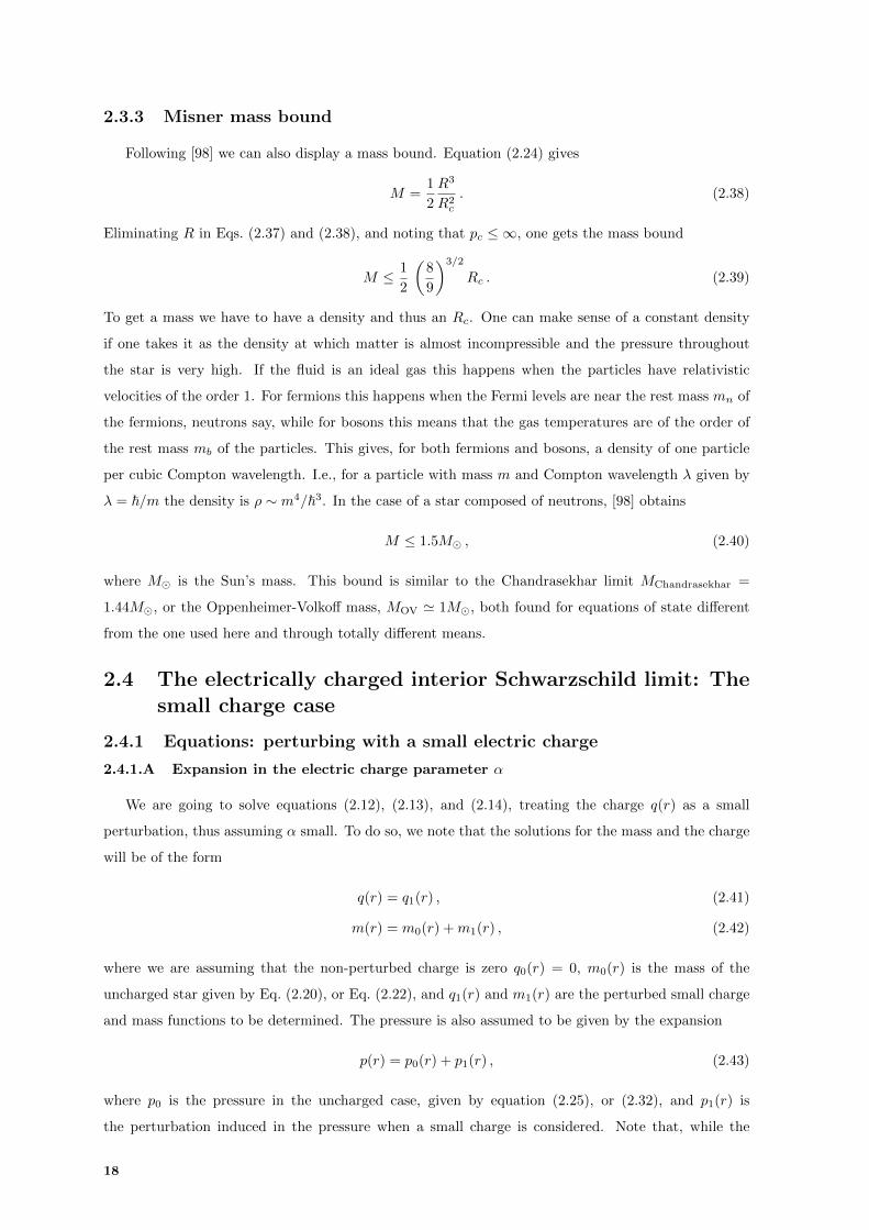
2.3.3 Misner mass bound

Following [98] we can also display a mass bound. Equation (2.24) gives

M =1

2

R3

R2c

. (2.38)

Eliminating R in Eqs. (2.37) and (2.38), and noting that pc ≤ ∞, one gets the mass bound

M ≤ 1

2

(8

9

)3/2

Rc . (2.39)

To get a mass we have to have a density and thus an Rc. One can make sense of a constant density

if one takes it as the density at which matter is almost incompressible and the pressure throughout

the star is very high. If the fluid is an ideal gas this happens when the particles have relativistic

velocities of the order 1. For fermions this happens when the Fermi levels are near the rest mass mn of

the fermions, neutrons say, while for bosons this means that the gas temperatures are of the order of

the rest mass mb of the particles. This gives, for both fermions and bosons, a density of one particle

per cubic Compton wavelength. I.e., for a particle with mass m and Compton wavelength λ given by

λ = ~/m the density is ρ ∼ m4/~3. In the case of a star composed of neutrons, [98] obtains

M ≤ 1.5M , (2.40)

where M is the Sun’s mass. This bound is similar to the Chandrasekhar limit MChandrasekhar =

1.44M, or the Oppenheimer-Volkoff mass, MOV ' 1M, both found for equations of state different

from the one used here and through totally different means.

2.4 The electrically charged interior Schwarzschild limit: Thesmall charge case

2.4.1 Equations: perturbing with a small electric charge

2.4.1.A Expansion in the electric charge parameter α

We are going to solve equations (2.12), (2.13), and (2.14), treating the charge q(r) as a small

perturbation, thus assuming α small. To do so, we note that the solutions for the mass and the charge

will be of the form

q(r) = q1(r) , (2.41)

m(r) = m0(r) +m1(r) , (2.42)

where we are assuming that the non-perturbed charge is zero q0(r) = 0, m0(r) is the mass of the

uncharged star given by Eq. (2.20), or Eq. (2.22), and q1(r) and m1(r) are the perturbed small charge

and mass functions to be determined. The pressure is also assumed to be given by the expansion

p(r) = p0(r) + p1(r) , (2.43)

where p0 is the pressure in the uncharged case, given by equation (2.25), or (2.32), and p1(r) is

the perturbation induced in the pressure when a small charge is considered. Note that, while the

18

boundary condition for the non-charged star was simply p(R) = p0(R) = 0, the boundary condition

for the charged star becomes

p0(R) + p1(R) = 0 . (2.44)

At this point, it will prove useful to introduce the dimensionless variable

x =r

Rc, (2.45)

where Rc is the characteristic length defined in Eq. (2.23). The expressions for the mass, charge, and

pressure in this new variable are generically defined as

m(x) =m(r)

Rc, q(x) =

q(r)

Rc, p(x) =

p(r)

ρ. (2.46)

From Eq. (2.45) we defined xs as the x at the surface, so that

xs =R

Rc. (2.47)

Accordingly, we define

m(xs) =M

Rc, q(xs) =

Q

Rc, p(xs) =

p(R)

ρ. (2.48)

2.4.1.B Calculation of the perturbed charge distribution q1

Expanding Eq. (2.13) for small α, we get in the x variable that

dq1

dx=

3

2α

x2

√1− x2

, (2.49)

up to first order in α. Solving the above equation subject to the condition q1(0) = 0 and expressing

the solution in terms of the variable x, results in

q1(x) =3

4α(

arcsinx− x√

1− x2). (2.50)

2.4.1.C Calculation of non-perturbed and perturbed masses

The unperturbed mass m0 can now be expressed simply as

m0(x) =x3

2. (2.51)

One can also find an expression for m1, namely,

m1(x) =3

8α2(

3x− x3 − 3√

1− x2 arcsinx). (2.52)

Indeed, from Eqs. (2.12) and (2.42), it is clear that the equation for the perturbed mass m1 is given

bydm1

dx=q1

x

dq1

dx. (2.53)

Inserting Eq. (2.50) into Eq. (2.53), we can integrate it using the boundary condition that the total

mass at the center of the star is m(0) = 0, which implies that m1(0) = 0 since Eq. (2.22), or Eq. (2.51),

satisfies m0(0) = 0. Doing this, we are led to Eq. (2.52).

19

2.4.1.D Equations for the pressures, solution for the zeroth order pressure, and calcu-lation of the perturbed pressure at the star’s radius

(i) Equations for the pressures

To find the equations for the pressures p0(x) and p1(x), we begin by expressing Eq. (2.14) for the total

pressure in terms of the variable x given in Eq. (2.45),

dp

dx=−

(1 + p(x))(3p(x)x/2 +m(x)/x2 − q2(x)/x3

)1− 2m(x)/x+ q2(x)/x2

+

+αq

x2√

1− 2m(x)/x+ q2(x)/x2. (2.54)

Now we can expanded the right side of the above equation in powers of α and retain the two lowest

terms. By doing so, and using the expansion (2.43) on the left side of Eq. (2.54) and Eqs. (2.41)-(2.42)

on the right hand side, we can equate the terms in equal powers of α, thus obtaining two differential

equations. The first one, obtained from the 0th power in α is

dp0(x)

dx= −

(1 + p0(x))(3p0(x)x/2 +m0(x)/x2

)1− 2m0(x)/x

, (2.55)

which is simply the differential equation for the unperturbed pressure. The second differential equation,

to first order in α2, is

dp1

dx=

αq1

x2√

1− 2m0/x− (1 + p0)(3p0x/2 + x/2)f1

(1− 2m0/x)2+

− p1(3p0x/2 + x/2) + (1 + p0)(3p1x/2 + f2)

(1− 2m0/x), (2.56)

which is the differential equation for the perturbed pressure p1, where, again, to shorten equations we

have dropped the dependence of variables p1, p0, m1, m0, and q1 on x, and we have also defined the

auxiliary functions f1 = f1(x) and f2 = f2(x) by

f1(x) =2m1(x)

x− q2

1(x)

x2, (2.57)

and

f2(x) =m1(x)

x2− q2

1(x)

x3. (2.58)

Ultimately, we want to obtain an equation for the radius R for which the central pressure blows

up. From Eq. (2.43), the central pressure is p(0) = p0(0) + p1(0). In Sec. 2.6 we show that p1(0) is

always finite. So we have to find a solution for the radius R at which p0(0) blows up.

(ii) Solution for the zeroth order pressure

We start by obtaining a solution for p0. Since the boundary condition has changed relatively to the

uncharged case, it is now given by Eq. (2.44), we cannot use a priori the form (2.32) for p0. We use

the solution to Eq. (2.55) without specifying any boundary condition. In the variable x, this means

p0(x) =

√1− x2 −A

3A−√

1− x2. (2.59)

where A is an integration constant. To find out what this constant is, we insert the above equation into

Eq. (2.44) and solve the resulting equation with respect to A. After expanding for the small charge

parameter α, and so for small p1, we are led to

A =√

1− x2s (1 + 2p1(xs)) , (2.60)

20

up to first order in the perturbed quantities. Then, the expression for p0, analogous to Eq. (2.32),

becomes

p0(x) = ρ

√1− x2 −

√1− x2

s (1 + 2p1(xs))

3√

1− x2s (1 + 2p1(xs))−

√1− x2

. (2.61)

Since p0(x) depends on p1(xs) in the denominator, we have to find p1(xs), i.e., we have to calculate

the perturbed pressure at the star’s radius.

(iii) Calculation of the perturbed pressure at the star’s radius

The equation for p1, Eq. (2.56), cannot be solved analytically for all x. However, we are only interested

in the value of p1 at the surface of the star. At this particular radius it is possible to obtain the exact

value of the perturbed pressure without ever solving Eq. (2.56). The reason for this is the fact that at

the star’s radius the pressure p(xs) = p0(xs) + p1(xs) is zero. Therefore, we can insert the boundary

condition p(xs) = 0 in the exact derivative of the pressure given by Eq. (2.54) and expand the resulting

equation for small α, giving

dp

dx

∣∣∣x=xs

= − m0(xs)

x2s(1− 2m0(xs)/xs)

+

− m0(xs)

1− 2m0(xs)/xs

(f1(xs)

x2s

+f2(xs)

m0(xs)

), (2.62)

up to first order, and where the auxiliary functions f1(x) and f2(x) are given by Eqs. (2.57) and (2.58),

respectively. Using the expansion (2.43) on the left side of Eq. (2.62), one can clearly see that there

is a compatibility condition which must be physically required, namely that, at the star surface, the

first term on the right side of Eq. (2.62) must be equal to Eq. (2.55) and the second term equal to

Eq. (2.56). Hence, we arrive at the two equations

3

2p2

0(xs) + 2 p0(xs) = 0 , (2.63)

and3

2p1(xs)p0(xs)xs + p0(xs)f2(xs) = 0 . (2.64)

These equations give two different solutions, namely, p0(xs) = 0 and p1(xs) = 0, or p0(xs) = − 43 and

p1(xs) = − 23x

−1s f2(xs). This latter solution does not satisfy the boundary condition (2.44) so the

unique valid solution is given by

p0(xs) = 0 , (2.65)

and

p1(xs) = 0 . (2.66)

2.4.1.E Equation for the minimum radius

We see that the central pressure p0(0) given in Eq. (2.61) is divergent when the following condition

holds,

3√

1− x2s (1 + 2p1(xs)) = 1 . (2.67)

Expanding it in α2 we arrive toxs

m0(xs)=

9

4− 9

8p1(xs) , (2.68)

21

valid in first order in α2. Using the expansion provided by Eq. (2.42), it can be shown that to first

order in α2, we havexs

m(xs)=

xsm0(xs)

− xsm1(xs)

m20(xs)

. (2.69)

Upon substituting Eq. (2.69) into Eq. (2.68) we conclude that

xsm(xs)

=9

4−(

9

8p1(xs) + xs

m1(xs)

m20(xs)

). (2.70)

Now, the minimum star radius R will not be just√

8/9Rc but will have corrections of order α2.

These corrections will induce changes of the order α4 in Eq. (2.70). Thus, we can set xs =√

8/9 in

Eq. (2.70), i.e.,

xsm(xs)

=9

4−

(9

8p1(xs) +

√8

9

m1(xs)

m20(xs)

), (2.71)

which is the equation we were looking for. Since m0(xs), m1(xs), and p1(xs) can be taken directly

from Eq. (2.51), Eq. (2.52), and Eq. (2.66), respectively, we can proceed to the final result. Indeed,

using Eqs. (2.51), (2.52), (2.66) in (2.71), we obtain

xsms

=9

4− 1.529α2 , (2.72)

up to order α2.

In converting from the variable x back to r, we use

xsm(xs)

=R

M. (2.73)

In addition, it can also be interesting to express α in terms of the total charge Q and mass M . The

following relation valid for small q1, or small α, can be found QM = q1(xs)

m0(xs)+m1(xs) = q1(xs)m0(xs) so that

q1(xs)

m0(xs)=

Q

M, (2.74)

up to order q1. We can then express α in terms of the ratio Q/M . Using Eqs. (2.50) and (2.51) in

Eq. (2.74), and solving the resulting equation for α, we obtain

1.641α =Q

M. (2.75)

2.4.2 The electric interior Schwarzschild limit: The R, M and Q relationfor small charge

We are now in a position to calculate the desired ratio (2.72) in terms of the quantities R, M and

Q and find the appropriate relation. Inserting Eq. (2.73) into Eq. (2.72) we find

R

M=

9

4− 1.529α2 , (2.76)

which is one form of the interior Schwarzschild limit for small charge.

Inserting Eq. (2.75) into Eq. (2.76) we get

R

M=

9

4− 0.568

Q2

M2, (2.77)

valid up to order Q2/M2. This is another form of the interior Schwarzschild limit for small charge.

22

We can also express the limit in terms of the horizon radius, r+, for the Reissner-Nordstrom metric.

The horizon radius is defined by Eq. (2.19), i.e., up to order Q2/M2 one has, r+ = M +√M2 −Q2 =

2M(

1− 14Q2

M2

). So,

R

r+=

9

8− 0.003

Q2

M2, (2.78)

up to order Q2/M2. Equation (2.78) is yet another form of the interior Schwarzschild limit for small

charge.

The electric interior Schwarzschild limit for small charge presented in various forms in Eqs. (2.76),

(2.77), and (2.78) is the main result of this work. All the three forms of the electric interior Schwarzschild

limit for small charge show that, in comparison with the uncharged case Eq. (2.37), the star can be

more compact. In particular, Eq. (2.78) shows that in the charged case the radius of the star can be

a bit nearer its own horizon.

In [61] these compact stars were studied numerically. AnR/M×Q/M relation was given numerically

for 0 ≤ Q/M ≤ 1. For small charge, Q/M 1, one can extract from the numerical calculations in

[61] that RM ' 2.25−0.6 Q2

M2 . This should be compared to our analytical calculation valid in first order

of Q/M , given here in Eq. (2.77), i.e., RM = 2.25 − 0.568 Q2

M2 . It shows that the numerical code used

in [61] is compatible with the analytical calculation. In that work [61] it was also shown numerically

that in the other extreme, namely, Q/M = 1, one would obtain a star at its own gravitational radius,

R/M = 1, i.e., an (extremal) quasiblack hole.

2.4.3 A mass bound

We can adapt the mass bound from section 2.3.3 to the small charge case. Indeed, from Eq. (2.42)

and the definition M ≡ m(R), we have at the boundary

M = m0(R) +m1(R) . (2.79)

Now, Eq. (2.51) at the boundary can be put in the form m0(R) = 12 Rc sin3 χs. So, Eq. (2.79) yields

M =1

2Rc sin3 χs +m1(R) . (2.80)

Since pc ≤ ∞, using equation (2.68) with p1(R) = 0, one obtains sin2 χs ≤ 89 , and the bound for the

non-perturbed mass m0 is given by m0(R) = 12Rc sin3 χs ≤ 1

2

(89

)3/2Rc. In order to obtain the bound

for m1, we have to substitute the bound sin2 χs ≤ 89 in equation (2.52). This is enough since we are

only working up to order α2. Thus, the mass bound for the small charge case is

M ≤ 1

2

(8

9

)3/2

Rc(1 + 0.679α2

). (2.81)

In the case of a compact star composed of neutrons in the incompressible state speckled with some

charged particles, we obtain

M ≤ 1.5M(1 + 0.679α2

), (2.82)

Comparing equation (2.82) with equation (2.40) we see that we can attain bigger mass on a charged

star. This is expected since the electrostatic repulsion is opposite to the gravitational force, which

means that we can put more mass on the star without it collapsing.

23

2.5 Conclusions

In this chapter we have studied the interior Schwarzschild limit of spherically symmetric star

configurations composed of a fluid with constant energy density ρ and with a small electrical charge

distribution ρe proportional to ρ, ρe = αρ with α 1. The exterior spacetime is described by the

Reissner-Nordstrom metric. We have found through an analytical scheme that due to the electric

charge distribution the limiting star configuration can have more mass and a smaller radius relatively

to the limiting star with zero charge. This is expected since the electric charge distribution has a

repulsive effect, adding to the pressure as a force that withstands the star. The analytical calculation

obtained is in accord with the results from the numerical code used in [61]. For stars containing some

type of dark matter in their interior there is the possibility that they possess a small but non-negligible

electric charge, in which case our analytical formula is opportune and can be confronted quantitatively

with observational data.

A related theme is the Buchdahl and the Buchdahl-Andreasson bounds. Buchdahl by imposing a

simple set of assumptions, namely, the spacetime is spherically symmetric, the star is made of a perfect

fluid, and the density is a nonincreasing function of the radius, found that the radius to mass relation

is R/M ≥ 9/4 [68]. Thus the Schwarzschild limit [104], i.e., the limiting R/M configuration when the

central pressure goes to infinity, is an instance that saturates the Buchdahl bound. Following the line

of reason of Buchdahl, [59] obtained a bound for the minimum radius of a star using the following

energy condition p + 2pT ≤ ρ where pT is the tangential pressure, p is the radial pressure and ρ is

the energy density. This bound, the Buchdahl-Andreasson bound, is given by RM ≤

9(1+√

1+3Q2/R2)2 .

Retaining terms in first order in Q2 one gets RM = 9

4 − 0.667 Q2

M2 . Thus, our configurations of constant

density and a charge distribution proportional to the energy density having RM = 9

4−0.568 Q2

M2 does not

saturate the bound. This raises the question of whether there are other types of charged matter that

can saturate the bound. One type is thin shells with an appropriate relation between surface energy

density and surface pressure [59]. Are there continuous (non-thin-shell) distribution configurations that

saturate the bound? It seems that, as the configurations analyzed here, the configurations studied in

[62, 75, 76] do not saturate the bound. It remains to be seen if the electrically charged configurations

analyzed in [81, 96] saturate the bound. For further study on bounds of electrically charged stars see

[64, 79, 109].

2.6 Appendix: Behaviour of the perturbed pressure for smallradius

Our goal is to compute the limit of infinite central pressure p(r = 0) in this charged case, so it

is important to analyze the behaviour of p1 for small radius x, x ∼ 0, which also means χ ∼ 0, and

r ∼ 0. We start by obtaining the perturbed charge, q1, for small radius expanding equation (2.50),

which gives

q1(x) ∼ αx3

2, (2.83)

24

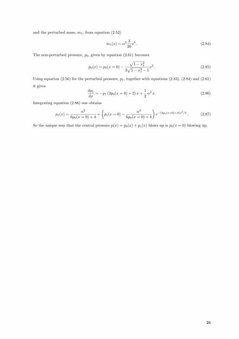
and the perturbed mass, m1, from equation (2.52)

m1(x) ∼ α2 3

20x5 . (2.84)

The non-perturbed pressure, p0, given by equation (2.61) becomes

p0(x) ∼ p0(x = 0)−√

1− x2s

3√

1− x2s − 1

x2 . (2.85)

Using equation (2.56) for the perturbed pressure, p1, together with equations (2.83), (2.84) and (2.61)

it givesdp1

dx∼ −p1 (3p0(x = 0) + 2)x+

1

2α2 x . (2.86)

Integrating equation (2.86) one obtains

p1(x) ∼ α2

6p0(x = 0) + 4+

(p1(x = 0)− α2

6p0(x = 0) + 4

)e−(3p0(x=0)+2)x2/2 . (2.87)

So the unique way that the central pressure p(x) = p0(x) + p1(x) blows up is p0(x = 0) blowing up.

25

3Dynamics of thin shells in a

(3+1)-dimensional asymptoticallyAdS spacetime

27

3.1 Introduction

The study of anti-de Sitter (AdS) spacetimes, i.e., spacetimes with a negative cosmological constant,

Λ < 0, is an important theme in general relativity field of sudy. Also, those spaces are used in theories

of quantum gravity, formulated in the terms of the string theory or M-theory [110]. In this chapter

we will focus in the (3+1)-dimensional AdS spacetime and we will study the dynamics of a particular

self-gravitating system: the thin matter shell.

A thin matter shell is a hypersurface which separates spacetime into two regions, the interior region

and the exterior region. Due to the development of a singularity in spacetime there are some conditions

that must be satisfied to ensure that the entire spacetime is a valid solution of Einstein’s equations:

the junctions conditions (see Appendix A). Their appropriate use leads us to pressure and rest mass

of the shell.

In this chapter we will adopt the following outline. In Sec. 3.2 we present the thin shell spacetime,

whereas in Sec. 3.3 we arrive to the junction conditions, which lead to the pressure and rest mass of

the shell. The no-trapped-surface condition and the weak and dominant energy conditions are also

discussed in Sec. 3.4. At the end we conclude in Sec. 3.5.

3.2 The thin shell spacetime

In 3+1 dimensions, Einstein’s equation with cosmological constant Λ is

Gαβ = 8πGTαβ + Λgαβ , (3.1)

where Gαβ is the Einstein tensor, G3 is the gravitacional constant in 2+1 dimensions, Tαβ is the

energy-momentum tensor and gαβ is the spacetime metric. We will choose units with the velocity of

light equal to one, c = 1, so that G has units of the inverse of mass. The greek indices run from 0, 1, 2, 3,

with 0 begin the time index. As we want to work in an AdS spacetime, with negative cosmological

constant, we define the AdS length l as

− Λ =1

l2. (3.2)

We assume a Schwarzschild AdS spacetime divided in two regions by a spherically symmetric thin

matter shell. The existence of the shell implies that certain conditions must be satisfied in order the

hypersuperface Σ that describes the evolution of the shell have a well defined geometry. The formalism

from [49, 111–113] gives two junction conditions, one for the induced metric hab, Eq. (A.16), on that

hypersuperface Σ and other for the extrinsic curvature of Σ, Kab in terms of a shell’s stress tensor Sab,

Eq. (A.35).

For a spherically symmetric (3+1)-dimensional spacetime one can write the line element on the

form

ds2 = −F±(r)dt2 +dr2

F±(r)+ r2

(dθ2 + sin2 θdφ2

). (3.3)

In the outer region, i.e. for r > R, where R is the shell’s radius and r is the radial Schwarzschild

solution usual coordinate, the metric is given by the Schwarzschild AdS line element, Eq. (3.3) with

F+(r) = 1− 2mG

r+r2

l2, (3.4)

28

where l2 = −1/Λ and m is the Arnowitt-Deser-Misner (ADM) mass.

In the inner region the metric is simply given by equation (3.3) with

F−(r) = 1 +r2

l2. (3.5)

An observer comoving with the shell describes Σ with parametric equations r = R(τ) and t = T (τ)

where τ is his proper time. Taking advantage of the spherical symmetry of the shell we can describe

Σ using the coordinates (τ ,θ,φ), which yields the following line element for the induced metric

ds2Σ = −dτ2 +R2

(dθ2 + sin2 θdφ2

). (3.6)

3.3 The thin shell gravitational junction conditions

Applying the first junction condition, Eq. (A.15), leads to

− F±T2 +

R2

F±= −1 , (3.7)

and the dot denotes differentiation with respect to τ .

With the line element for the hypersurface Σ, Eq. (3.3), the non-null components of the extrinsic

curvature are

Kτ±τ =

˙β±

R, (3.8)

Kθ±θ = Kφ

±φ =β±R, (3.9)

where β± =√F±(r) + R2. Using the second junction condition, equation (A.35) one obtains the

non-null components of the stress-energy tensor of the shell

Sττ =β+ − β−

4πGR, (3.10)

Sθθ = Sφφ =β+ − β−8πGR

+β+ − ˙β−

8πGR. (3.11)

Since we assume the shell to be a perfect fluid, the stress-energy tensor is of the form Sab = (σ +

p)uaub + phab , where σ is the surface density and p is the superficial pressure. Defining the shell rest

mass as M = 4πR2σ and imposing that the shell is static, so that R = R = 0, gives

M =R

G

(√1 +

R2

l2−√

1 +R2

l2− 2mG

R

), (3.12)

p =1

8πGR

√

1 +R2

l2− 2mG

R−√

1 +R2

l2+

mG

R+R2

l2√1 +

R2

l2− 2mG

R

−

R2

l2√1 +

R2

l2

. (3.13)

We can solve Eq. (3.12) for the ADM mass m

m = M

√1 +

R2

l2− GM2

2R. (3.14)

29

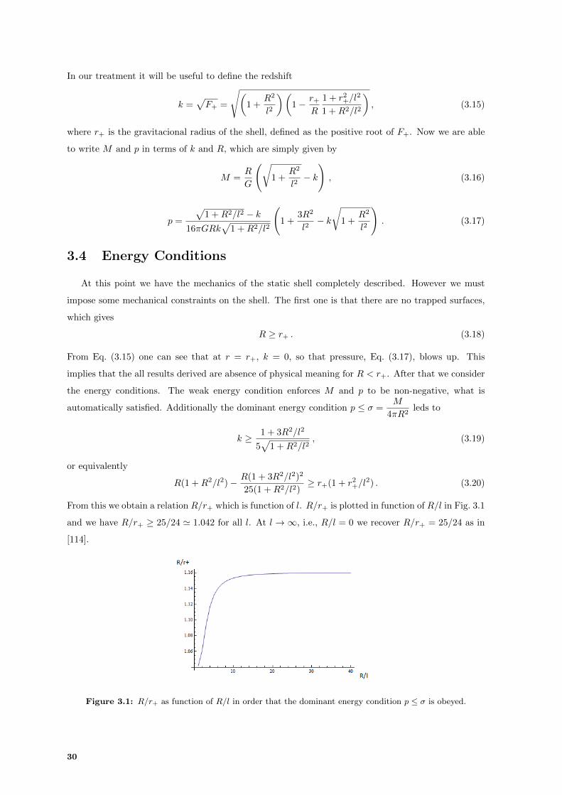
In our treatment it will be useful to define the redshift

k =√F+ =

√(1 +

R2

l2

)(1− r+

R

1 + r2+/l

2

1 +R2/l2

), (3.15)

where r+ is the gravitacional radius of the shell, defined as the positive root of F+. Now we are able

to write M and p in terms of k and R, which are simply given by

M =R

G

(√1 +

R2

l2− k

), (3.16)

p =

√1 +R2/l2 − k

16πGRk√

1 +R2/l2

(1 +

3R2

l2− k√

1 +R2

l2

). (3.17)

3.4 Energy Conditions

At this point we have the mechanics of the static shell completely described. However we must

impose some mechanical constraints on the shell. The first one is that there are no trapped surfaces,

which gives

R ≥ r+ . (3.18)

From Eq. (3.15) one can see that at r = r+, k = 0, so that pressure, Eq. (3.17), blows up. This

implies that the all results derived are absence of physical meaning for R < r+. After that we consider

the energy conditions. The weak energy condition enforces M and p to be non-negative, what is

automatically satisfied. Additionally the dominant energy condition p ≤ σ =M

4πR2leds to

k ≥ 1 + 3R2/l2

5√

1 +R2/l2, (3.19)

or equivalently

R(1 +R2/l2)− R(1 + 3R2/l2)2

25(1 +R2/l2)≥ r+(1 + r2

+/l2) . (3.20)

From this we obtain a relation R/r+ which is function of l. R/r+ is plotted in function of R/l in Fig. 3.1

and we have R/r+ ≥ 25/24 ' 1.042 for all l. At l → ∞, i.e., R/l = 0 we recover R/r+ = 25/24 as in

[114].

Figure 3.1: R/r+ as function of R/l in order that the dominant energy condition p ≤ σ is obeyed.

30

3.5 Conclusions

In this chapter we have studied the dynamics of a thin matter shell composed of a perfect fluid

in a (3+1)-dimensional AdS spacetime. Through the junction conditions we have arrived to the rest

mass and the pressure of the shell. We also have analyzed the weak and dominant energy conditions

of the system. Finally, the results of this chapter will be useful for study the thermodynamics of this

system, which will be done in Chapter 5

31

4Dynamics of rotating thin shells in

a (2+1)-dimensional asymptoticallyAdS spacetime

33

4.1 Introduction

Sometimes it is interesting to reduce the spatial dimension to 2 and study general relativiy in

(2+1)-dimensions. This decrease in dimensionality reduces the degrees of freedom and simplifies the

calculations, although maintaining the essential physical features. The interest in (2+1)-dimensional

spacetimes suffered an increment after the discovery of a black hole solution in spacetimes asymptoti-

cally AdS, the Banados-Teitelbom-Zanelli (BTZ) black hole [47] [48].

In this chapter we are going to study the dynamics of a thin matter shell (see Appendix A) in a

(2+1)-dimensional rotating AdS spacetime, i.e., a ring dividing two vacuum regions, the interior region

and the exterior region. The exterior spacetime is BTZ and thus asymptotically AdS and inside the

ring the spacetime is flat AdS. Our approach to the dynamics of the shell will be equivalent to the

ones [51], [50] and [49], for a (3+1)-dimensional rotating shell.

In this chapter we will adopt the following outline. In Sec. 4.2 we present the thin shell spacetime.

In Sec. 4.3 we present the junction conditions and we obtain the linear energy density, pressure and

angular velocity of the shell, in the slowly rotating limit, whereas in Sec. 4.4 we arrive to the same

quantities for the rotating general case. Finally we conclude in Sec. 4.5.

4.2 The thin shell spacetime

In 2+1 dimensions, Einstein’s equation is

Gαβ = 8πG3Tαβ + Λgαβ , (4.1)

where Gαβ is the Einstein tensor, G3 is the gravitacional constant in 2+1 dimensions, Λ is the cosmo-

logical constant, Tαβ is the energy-momentum tensor and gαβ is the spacetime metric. We will choose

units with the velocity of light equal to one, c = 1, so that G3 has units of the inverse of mass. The

greek indices run from 0, 1, 2, with 0 begin the time index. Since we want to work in an AdS spacetime,

with negative cosmological constant, we define the AdS length l as in Eq. (3.2)

We consider a timelike shell with radius R, i.e., a ring, in a (2+1)-dimensional spacetime. This

ring divides spacetime into two regions, an inner region and an outer one.

The exterior metric is given by the BTZ line element [47]

ds2+ = g+

αβdxα+dx

β+ =−

(r2

l2− 8G3m

)dt2+ (4.2)

+dr2(

r2

l2− 8G3m+

16J2G23

r2

)− 8G3Jdt+dφ+ r2dφ2, r ≥ R ,

written in exterior coordinate system xα+ = (t+, r, φ), where J is the shell’s angular momentum and

m is the Arnowitt-Deser-Misner (ADM) mass. On the other hand, the interior region is flat AdS

spacetime with metric given by

ds2− = g−αβdx

αdxβ =− ρ2

l2dt2− +

l2

ρ2dρ2 + ρ2dψ2 ρ ≤ R , (4.3)

34

written in interior coordinate system xα− = (t−, ρ, ψ).

4.3 The thin shell gravitational junction conditions: slowlyrotating limit

We start by analyzing the dynamics of this rotating shell by taking the slowly rotating limit. This

means we will work consistently to first order in J , the exterior spacetime angular momentum. The

exterior metric, Eq. (4.2), becomes

ds2+ = g+

αβdxαdxβ =−

(r2

l2− 8G3m

)dt2+ (4.4)

+dr2(

r2

l2− 8G3m

)− 8G3Jdt+dφ+ r2dφ2, r ≤ R .

The induced metric, as viewed from the exterior region, is obtained by setting r = R in Eq. (4.4),

which gives

ds2Σ =−

(R2

l2− 8G3m

)dt2+ − 8G3Jdt+dφ+R2dφ2 . (4.5)

One can remove the off-diagonal term of the induced metric through a transformation to a co-rotating

frame. Accordingly we define a new polar coordinate ψ by

ψ = φ− Ωt+ , (4.6)

which makes the induced metric, Eq. (4.5), diagonal if Ω is choosen to be

Ω =4G3J

R2. (4.7)

Note that this polar coordinate ψ is precisely the interior polar coordinate, as in Eq. (4.3). Thus, in

coordinates (t, ψ), where we chose t ≡ t+, the induced metric is written as

ds2Σ =−

(R2

l2− 8G3m

)dt2 +R2dψ2 . (4.8)

The induced metric, as viewed from the interior region, is obtained by setting ρ = R in Eq. (4.3),

which gives

ds2Σ =− R2

l2dt2− +R2dψ2 . (4.9)

Applying the first junction condition, Eq. (A.15), leads to(R2

l2− 8G3m

)dt2 =

R2

l2dt2− , (4.10)

so that we can write the interior metric as

ds2− =− ρ2

l2

(R2/l2 − 8G3m

)R2/l2

dt2 +l2

ρ2dρ2 + ρ2dψ2 . (4.11)

35

Now we are in conditions to compute the extrinsic curvature as viewed from both sides of the shell,

given by Eq. (A.32). As seen from the exterior region

Ktt =

−R

l2

√−8G3m+

R2

l2

, (4.12)

Ktψ =

−4G3J/R√−8G3m+

R2

l2

, (4.13)

Kψt =

4G3J

√−8G3m+

R2

l2

R3, (4.14)

Kψψ =

√−8G3m+

R2

l2

R. (4.15)

As seen from the shell’s interior

Ktt = Kψ

ψ =1

l, (4.16)

are the only non-vanishing components. Therefore the components of the surface stress-energy tensor

are

Stt =−1

8πG3l

(1− l

R

√−8G3m+

R2

l2

), (4.17)

Stψ =−J√−8G3m+

R2

l2

2πR3, (4.18)

Sψt =J

2πR

√−8G3m+

R2

l2

, (4.19)

Sψψ =−1

8πG3l

−1 +R

l

1√−8G3m+

R2

l2

. (4.20)

This is not the surface stress-energy tensor of a perfect fluid so we will attempt to write it in the

perfect fluid form

Sab = λuaub + p(hab + uaub

), (4.21)

where hab is the induced metric from either outer or inner regions, λ is a surface density, p is a surface

pressure and ua is a velocity field. Recognizing that the shell must move rigidly in the ψ direction

with an uniform angular velocity ω implies that the velocity vector is expressed as

ua = γ(ta + ωψa) . (4.22)

Then one obtains

γ =

√√√√ −1

−8G3m+R2

l2

, (4.23)

λ = −Stt =1

8πG3l

(1− l

R

√−8G3m+

R2

l2

), (4.24)

36

p = Sψψ =1

8πG3l

−1 +R

l

1√−8G3m+

R2

l2

. (4.25)

At this point is useful to introduce the gravitacional radius r+ and the Cauchy radius r− of the shell,

with subsequent explicit expression

r± = 2l

√G3m±

√G2

3m2 − J2G2

3

l2. (4.26)

From transformation of Eq. (4.21) one also obtains

ω =−Sψt

Sψψ − Stt=

r−r+l− r−r+

lR2. (4.27)

The shell’s angular velocity as measured in the nonrotating frame is Ωshell = ω + Ω, given by

Ωshell =r−lr+

, (4.28)

which coincides with the BTZ spacetime angular velocity [52]. Also, in the slowly rotating limit, λ

and p, are equal to the ones of the non-rotating BTZ thin matter shell [53]. We define the shell’s rest

mass as

M = 2πRλ , (4.29)

so that, using Eq. (4.24)

M =R

4G3l

(1− l

R

√−8G3m+

R2

l2

). (4.30)

Therefore we can solve Eq. (4.30) for the ADM mass m

m = −2G3M2 +

R

lM . (4.31)

It will be also useful to define the quantity

k =

√(1−

r2+

R2

)(1−

r2−R2

)=

√(1−

r2+

R2

), (4.32)

up to order J2. Now we are in position to write M and p in terms of k and R

M =R

4G3l(1− k) , (4.33)

p =1

8πG3l

(1

k− 1

). (4.34)

4.3.1 Energy conditions

At this point we have the dynamical problem solved, however we need to impose some mechanical

constraints and energy conditions on the shell. The first constraint is that the shell must be outside

any trapped surface in order for the spacetime defined to make sense. This constraint yields

R ≥ r+ , (4.35)

and means the shell is outside its own gravitational radius. The next constraint is the weak energy

condition, which is automatically satisfied since we impose λ and p non-negative. Futhermore the

dominant energy condition, p ≤ λ, leads to the condition

r+

R= 0 . (4.36)

37

4.4 The thin shell gravitational junction conditions: exact so-lution

Now we analyze exactly the dynamic of this rotating shell. The induced metric, as viewed from

the exterior region, is obtained by setting r = R in Eq. (4.2), which gives

ds2Σ =−

(R2

l2− 8G3m

)dt2+ − 8G3Jdt+dφ+R2dφ2 . (4.37)

To remove the off-diagonal term in Eq. (4.37), we go to a co-rotating frame, defining the new polar

coordinate ψ by

ψ = φ− Ωt+ , (4.38)

which makes the induced metric, Eq. (4.37), diagonal if Ω is choosen to be

Ω =4G3J

R2. (4.39)

Therefore, in coordinates (t, ψ), where we chose t ≡ t+, the induced metric is written as

ds2Σ =−

(R2

l2− 8G3m+

16J2G23

R2

)dt2 +R2dψ2 . (4.40)

On the other hand the induced metric, as viewed from the interior region, is obtained by setting ρ = R

in Eq. (4.3), which gives

ds2Σ =− R2

l2dt2− +R2dψ2 . (4.41)

Applying the first junction condition, Eq. (A.15), yields(R2

l2− 8G3m+

16J2G23

R2

)dt2 =

R2

l2dt2− , (4.42)

so that we can write the interior metric as

ds2− =− ρ2

l2

(R2/l2 − 8G3m+

16J2G23

R2

)R2/l2

dt2 +l2

ρ2dρ2 + ρ2dψ2 . (4.43)

Using Eq. (A.32) the components of the extrinsic curvature are

Ktt =

−R

l2

√−8G3m+

R2

l2+

16J2G23

R2

(1− 16J2G2

3

R2

), (4.44)

Ktψ =

−4G3J/R√−8G3m+

R2

l2+

16J2G23

R2

, (4.45)

Kψt =

4G3J

√−8G3m+

R2

l2+

16J2G23

R2

R3, (4.46)

Kψψ =

√−8G3m+

R2

l2+

16J2G23

R2

R. (4.47)

As seen from the shell’s interior the only non-vanishing components are

Ktt = Kψ

ψ =1

l. (4.48)

38

Using the second junction condition, Eq. (A.35), the components of the surface stress-energy tensor

are

Stt =−1

8πG3l

(1− l

R

√−8G3m+

R2

l2+

16J2G23

R2

), (4.49)

Stψ =−J√−8G3m+

R2

l2+

16J2G23

R2

2πR3, (4.50)

Sψt =J

2πR

√−8G3m+

R2

l2+

16J2G23

R2

, (4.51)

Sψψ =1

8πG3l

−1 +R

l

1√−8G3m+

R2

l2+

16J2G23

R2

. (4.52)

We will attempt to write the surface stress-energy tensor in a perfect fluid form as done in Eqs. (4.21)-

(4.22). Also the shell must move rigidly in the ψ direction with an uniform angular velocity ω implying

that the velocity vector is expressed as

ua = γ(ta + ωψa) . (4.53)

Therefore, one obtains

λ =M

2πR=

1

8πG3l(1− k) +

r2+r

2−

R4

(1−R2/r2

+

)8πG3lk

, (4.54)

p =1

8πG3l

[1

k

(1−

r2+r

2−

R4

)− 1

]+r2−R2

(R2 − r2

+

)8πG3lk

(r2+ − r2

−) (−2r2

−r2+

R4+r2+ + r2

−R2

), (4.55)

ω =r−r+l− r−r+

lR2, (4.56)

where Eq. (4.32) was used. The shell’s angular velocity measured in the nonrotating frame is Ωshell =

ω + Ω, given by

Ωshell =r−lr+

, (4.57)

which coincides with the BTZ spacetime angular velocity [52].

4.4.1 Energy conditions

Finally we need to impose some mechanical constraints and energy conditions on the shell. The

constraint that the shell must be outside any trapped surface yields

R ≥ r+ . (4.58)

The weak energy condition is automatically satisfied since we impose λ and p non-negative.

Futhermore the dominant energy condition, p ≤ λ is satisfied if

k ∈ [k−, k+] , (4.59)

with k± = 1±√

1− a and

a =

(1−

r2+r

2−

R4

)+r2−R2

[(1− r2

+/R2)

+R2 − r2

+

r2+ − r2

−

(−

2r2−r

2+

R4+r2+ + r2

−R2

)](4.60)

39

4.5 Conclusions

In this chapter we have obtained the dynamics of a thin matter shell in a (2+1)-dimensional

rotating AdS spacetime. By using the junction conditions we have arrived to the rest mass, pressure

and angular velocity of the shell. First we have done it for the slowly rotating limit and after that we

have obtained the exact solution. We also have analyzed the weak and dominant energy conditions

of the system. Note that, because of rotation, the shell’s surface energy-stress tensor was not in the

form of a perfect fluid. We overcame this difficulty by attempting to write the tensor in a perfect fluid

form like in [49–51]. The results of this chapter will be useful for the study of thermodynamics on this

system, which will be the theme of work in Chapter 6.

40

5Entropy of thin shells in a

(3+1)-dimensional asymptoticallyAdS spacetime and the

Schwarzschild-AdS black hole limit

41

5.1 Introduction

In this chapter we are interested in the (3+1)-dimensional AdS spacetime. In particular we are

going to focus our attention in the thermodynamics of a particular gravitating system: a thin matter

shell, of which dynamics have been studied in chapter 3.

Once we obtained the entropy from the thermodynamics approach, we can take the black hole [40]

limit, i.e., the shell can be taken to its gravitational radius, obtaining the black hole entropy. Thus, the

black hole thermodynamic properties can be attained using a much more simplified computation than

the usual black hole mechanics. This idea was developed by Martinez [114] and is going to be applied

throughout this chapter, which will generalize the result from [114], by adding a negative cosmological

constant.

The Schwarzschild AdS black hole is a semi classical system, spherically symmetric, with a Bekenstein-

Hawking entropy SBH = 14Ah

lp, where Ah is the horizon area, Ah = 4πr2

+, r+ is the horizon radius and

lp is the Planck length given by lp =√G ~, with G being the gravitational constant and ~ Planck’s

constant. We will use units c = kB = 1, where c is the vacuum speed of light and kB is the Boltzmann

constant. That black hole has a Hawking temperature given by TH = ~ 1+3r2+/l2

4πr+[116].

We will adopt the following outline. Sec. 5.2 is dedicated to the thermodynamics generics of the

shell, to present the entropy representation and the state variables shell’s proper mass, M , and area,

A. In Sec. 5.3 we show the pressure equation of state in terms of the proper mass and radius of

the shell, and we obtain the temperature equation of state. In Sec. 5.4 we obtain shell’s entropy

up to an arbitrary function of the gravitational radius. We also push the shell to its gravitacional

radius and equate that function to the inverse Hawking temperature. Then we found that the entropy

is precisely Bekenstein-Hawking entropy of the Schwarzschild AdS black hole. In Sec. 5.5 we take a

phenomenological expression for that arbitrary function which allows us to compute the shell’s entropy.

After that we analyze the thermodynamic stability and we conclude in Sec. 5.6.

5.2 Thermodynamics and stability conditions for the thin shell

Proceeding to the computation of the entropy of the shell, we assume the entropy S to be a function

of the shell’s rest mass M and area A = 4πR2, i.e.,

S = S(M,A) . (5.1)

Note that the number of particles N is considered constant. We also consider the assumption that the

shell is a hot shell, i.e., it has a well defined local temperature T . Thus the first law of thermodynamics

can be written as

TdS = dM + pdA . (5.2)

It is far-reaching to note that the temperature plays the role of an integration factor, which implies

the following integrability condition (∂β

∂A

)M

=

(∂βp

∂M

)A

, (5.3)

42

for the sake of guarantee that the differential dS is exact and where we define the inverse temperature

β = 1/T . To find the entropy S one needs two equations of state, which are

p = p(M,A) , (5.4)

β = β(M,A) . (5.5)

There is then the achievability of studying the local intrinsic stability of the shell, which is assured

if the following inequalities hold simultaneously (see [115] [119])(∂2S

∂A2

)M

≤ 0 , (5.6)

(∂2S

∂M2

)A

≤ 0 , (5.7)

(∂2S

∂M∂A

)2

−(∂2S

∂A2

)(∂2S

∂M2

)≤ 0 . (5.8)

5.3 The two equations of state: equations for the pressure andtemperature

5.3.1 The two independent thermodynamic variables

Although the first law of thermodynamics, Eq. (5.2), is simpler when expressed using the area A,

we are going to use it in terms of the shell’s radius R, related to A by

R =

√A

4π. (5.9)

At this point our thermodynamics variables are (R,M).

5.3.2 The pressure equation of state

The pressure equation of state, p(M,R), is given through Eq. (3.17)

p(M,R) =

√1 +R2/l2 − k(M,R)

16πGRk(M,R)√

1 +R2/l2

(1 +

3R2

l2− k(M,R)

√1 +

R2

l2

), (5.10)

which is equivalent to

p(M,R) =GM2

16πR2(R√

1 +R2/l2 −GM) +

R2

l2M/√

1 +R2/l2

8πR2(√

1 +R2/l2 −GM/R) . (5.11)

5.3.3 The temperature equation of state

Futhermore, to determine the temperature equation of state Eq. (5.5), we apply the integrability

condition Eq. (5.3), which, using the variables (r+, R), turns into(∂β

∂R

)r+

= β1 +R2/l2 − k2

2Rk2+ β

R

k2l2, (5.12)

which the analytic solution is found to be

β(r+, R) = b(r+)k(r+, R) . (5.13)

43

Therefore we obtain the Tolman’s formula for the temperature of a body in curved spacetime [120].

b(r+) is an arbitrary function of the gravitacional radius r+ and is also the inverse temperature of

the shell if its radius is infinite b(r+) = β(r+,∞). This function remains arbitrary unless we specify

the configurations for the shell’s matter fields. It is important to note that b is a function of (M,R),

through the variable r+ = r+(M,R).

5.4 Entropy of the thin shell

At this point we have assembled all we demand to compute the entropy of the shell. First we note

that

p = − 1

8πR

(∂M

∂R

)r+

, (5.14)

from Eqs. (3.15), (3.16) and (3.17). Thus, changing variables from (M,A) to (r+, R), Eq. (5.2) becomes

dS = β(r+, R)1

2k(r+, R)G

(1 +

3r2+

l2

). (5.15)

Combining Eqs. (5.15) and (5.13) gives the differential of the entropy, only in terms of r+

dS =b(r+)

2G

(1 +

3r2+

l2

)dr+ . (5.16)

This implies that

S = S(r+) , (5.17)

i.e., the entropy S is a function of r+ alone. However S is a function of (M,R), with the functional

dependence being through r+(M,R).

In order to obtain a specific expression for the entropy, we need to specify the function b(r+).

5.4.1 The temperature equation of state and the entropy

Let us specify a particular function for b(r+) of the shell, given by the following dependence

b(r+) = γr+

1 + 3r2+/l

2, (5.18)

with γ being some constant with units of inverse mass times inverse radius. This constant is determined

by the properties of the shell itself. Inserting this result, Eq. (5.18), in Eq. (5.16) yields the entropy

differential for that particular shell

dS =γ

2Gr+dr+ . (5.19)

Then the entropy of the shell is

S =γ

4Gr2+ + S0 , (5.20)

where S0 is an integration constant. When the shell vanishes (M = r+ = 0) it seems physically

reasonable to assume that the entropy must be zero, which implies that S0 = 0.

44

5.4.2 The black hole limit

Straightaway we can take the black hole limit R→ r+ like in [53, 114, 119]. As the shell is drawins

near its gravitacional radius, we have to consider quantum fields, whose backreaction will diverge unless

we take the temperature of the shell at infinity, b(r+)−1, to be equal to the Hawking temperature

TH =~

4π

1 + 3r2+/l

2

r+, (5.21)

so that

b(r+) =1

TH=

4π

~r+

1 + 3r2+/l

2, (5.22)

which means that γ depends only on fundamental constants

γ =4π

~. (5.23)

Implanting this b(r+) in Eq. (5.16) and integrating gives the entropy of the shell in the black hole

limit

S(r+) =πr2

+

l2p=A+

4l2p, (5.24)

where lp =√G~ is the Planck length. One can observe that Eq. (5.24) is precisely the Bekenstein-

Hawking entropy for a black hole, forasmuch as A+ = Ah is the black hole horizon area.

5.5 Another specific equation of state for the temperature ofthe thin matter shell: entropy and stability


For the sake of gathering an expression for the entropy, one have to specify a suitable equation of

state for b(r+). The simplest ansatz is the following power law

b(r+) = 2Gηra+ . (5.25)

Inserting Eq. (5.25) into Eq. (5.16) and integrating yields

S = ηra+1+

(1

a+ 1+

3r2+

l21

a+ 3

)+ S0 , (5.26)

for a > −1 and where S0 is a constant. It is reasonable to assume that a zero mass shell must possess

zero entropy, so that a > −1 and S0 = 0.

5.5.2 The stability conditions for the specific temperature ansatz

After that we analyze the shell’s stability through Eqs. (5.6)-(5.8). The first inequality, Eq. (5.6),

gives

a ≤ 0 ∨(a > 0 ∧ 2ak2

1 + 3r2+/l

2≤ r+

R

). (5.27)

The next condition, Eq. (5.7), yields(√1 +R2/l2 − k

)(−3r+

R+ a

(√1 +R2/l2 − k

) l2

3r2+

(5.28)

+ a2R2

3r2+

√1 +R2/l2

)− 2R2

l2Rr+

l21

(1 +R2/l2)3/2≤ 0 .

45

Finally, from Eq. (5.8) one obtains the following inequation(2ak2

1 + 3r2+/l

2− r+

R

)GM

2R

[−2R2

l2Rr+

l21

(1 +R2/l2)3/2

−3r+

R

GM

R+ a

(GM

R+

2R2/l2√1 +R2/l2

)GM

R

1

1 + 3r2+/l

2

]

−

[(GM

R+

R2/l2√1 +R2/l2

)(r+

R+

ak

1 + 3r2+/l

2

GM

R

)

+ak

1 + 3r2+/l

2

GM

R

R2/l2√1 +R2/l2

]2

≥ 0 , (5.29)

where GM/R =√

1 +R2/l2 − k, by Eq. (3.16).

5.6 Conclusions

In this chapter we have generalized the Martinez [114] work on the thermodynamics of a self-

gravitating (3+1)-dimensional thin matter shell by adding a negative cosmological constant. Inside the

shell the spacetime is described by the AdS metric, outside is given by the Schwarzschild AdS metric,

and it is asymptotically AdS. We have obtained the rest mass and pressure using the junction conditions

in Chapter 3, which led to a differential for the entropy, by using the first law of thermodynamics. We

have found the inverse temperature b(r+) and the entropy to be functions of r+ alone. However this

r+ is itself a function of the thermodynamic variables M and R.

We have choosed an ansatz for the thermal equation of state, which led to Eq. (5.26) for the

entropy of the shell. The complexity in the thermodynamic stability analysis, Eqs. (5.27)-(5.29) forbid

the possibility of obtaining a range for the parameter a and for R, as in [114].

In the case where the shell was pushed to its gravitacional radius and where the inverse temperature

was equal to the inverse of the Hawking temperature we found that the entropy was equal to the

Bekenstein-Hawking entropy of a Schwarzschild AdS black hole. One should note that the Hawking

temperature is a quantum result that was inserted by hand on the entropy, which was obtained only

by thermodynamics of spacetime, without specifying the material degrees of freedom.

46

6Entropy of slowly rotating thin

shells in a (2+1)-dimensionalasymptotically AdS spacetime and

the BTZ black hole limit

47

6.1 Introduction

In this chapter we will focus in the thermodynamics of a slowly rotating thin matter shell in a

(2+1)-dimensional asymptotically AdS spacetime, of which dynamics have been studied in chapter 4.

We intend to find the shell’s entropy, study its thermodynamic stability, and take the black hole[53,

114, 119] limit, i.e., when the shell is taken to its gravitational radius and obtain the corresponding

entropy. We will adopt the method developed by Martinez [114] and obtain the BTZ black hole, [47],

thermodynamic properties with a much more straightforward computation than the usual black hole

mechanics.

The BTZ black hole is a semi classical system with a Bekenstein-Hawking entropy SBH = 14Ah

l2p,

where Ah is the horizon area, Ah = 4πr2+, r+ is the horizon radius and lp is the Planck length given by

lp =√G ~, with G being the gravitational constant and ~ Planck’s constant. In this chapter we use

units c = kB = 1, where c is the vacuum speed of light and kB is the Boltzmann constant. The black

hole has a Hawking temperature given by TH =~

2πl2r2+ − r2

−r+

and an angular velocity ωBH =r−lr+

[52].

This chapter is organized as follows. Sec. 6.2 presents the thermodynamics generics of the shell,

the entropy representation and the state variables which are shell’s proper mass, M , area, A and

shell’s angular momentum J . In Sec. 6.3 we give the pressure equation of state in terms of the

thermodynamic variables. We also obtain the temperature equation of state and the angular velocity

for the first law of thermodynamics. In Sec. 6.4 we arrive to shell’s entropy with an arbitrary function

of the gravitational radius to be specify. Then we take the black hole limit and we arrive to the

Bekenstein-Hawking entropy of the BTZ black hole. In Sec. 6.5 we prescribe a phenomenological

expression for the arbitrary function which leads us to a complete expression of the shell’s entropy.

With that arbitrary function specified we analyze the thermodynamic stability. Finally we conclude

in Sec. 6.6.

6.2 Thermodynamics and stability conditions for the thin shell

At this moment we have to consider that the shell as a temperature T as measured locally, i.e., is

a hot shell, and has an entropy S.

In the formalism stated in [115], the entropy S of a system is given in terms of the state independent

variables, which we must designate, in order to obtain the complete thermodynamics description of the

system. The natural choice of variables is (M,A, J), i.e, the proper local mass M , the ring perimeter

A and the angular momentum J , so that

S = S(M,A, J) . (6.1)

With this variables, we can write the first law of thermodynamics as

TdS = dM + p dA− ωdJ , (6.2)

where T , p and ω are the temperature, the pressure and the angular velocity, respectively. For the

sake of finding S, one has to perceive the equations of state for the quantities that appear in Eq. (6.2)

48

and that are not thermodynamic variables, i.e.,

p = p(M,A, J) , (6.3)

ω = ω(M,A, J) , (6.4)

and

β = β(M,A, J) , (6.5)

where β = 1/T is the inverse temperature.

In order to Eq. (6.2) for dS to be an exact differential, there are three integrability condition to be

satisfied, as follow (see [115, 119]) (∂β

∂A

)M,J

=

(∂βp

∂M

)A,J

. (6.6)

(∂β

∂J

)M,A

= −(∂βω

∂M

)A,J

. (6.7)

(∂βp

∂J

)M,A

= −(∂βω

∂A

)M,J

. (6.8)

There is also the possibility of studying the local intrinsic thermodynamical stability of the shell,

which is guaranteed as long as the entropy of the system stays in a maximum. Following [115], if the

inequalities (∂2S

∂M2

)A,J

≤ 0 , (6.9)

(∂2S

∂A2

)M,J

≤ 0 , (6.10)

(∂2S

∂J2

)M,A

≤ 0 , (6.11)

(∂2S

∂M2

)(∂2S

∂A2

)−(

∂2S

∂M∂A

)2

≥ 0 , (6.12)

(∂2S

∂A2

)(∂2S

∂J2

)−(∂2S

∂A∂J

)2

≥ 0 , (6.13)

(∂2S

∂M2

)(∂2S

∂J2

)−(

∂2S

∂M∂J

)2

≥ 0 , (6.14)

(∂2S

∂M2

)(∂2S

∂J∂A

)−(

∂2S

∂M∂A

)(∂2S

∂M∂J

)≥ 0 , (6.15)

are satisfied, then stability is guarantee.

49

6.3 The three equations of state: equation for the pressure,equation for the temperature and equation for angular ve-locity

6.3.1 The three independent thermodynamic variables

We define shell’s rest mass M as

M = 2πRλ , (6.16)

where λ is given by Eq. (4.24).

Second, we note that

A = 2πR , (6.17)

so that the variables perimeter A and the radius R can be directly swapped as independent variables.

At this point we choose our thermodynamics variables as (M,R, J).

6.3.2 The pressure equation of state

By combining Eqs. (4.25) and (4.24) we arrive to the seeked equation of state (6.3)

p(M,R, J) = p(M,R) =1

8πG3l

1

1− 4G3Ml

R

− 1

, (6.18)

where A has been swapped with R, by Eq. (6.16). This equation follows exclusively from the spacetime

structure and does not depend on the matter composing the shell. This can be observed since the

equation is derived only by using gravitational considerations and the junction conditions on the ring,

without ever specifying the matter fields. It is the same as obtained in [53].

6.3.3 The temperature equation of state

Now we turn our attention to the other equation of state, Eq. (6.5), for β(M,R, J). This equation

is obtained from the first integrability condition, Eq. (6.6), by changing from variables (M,A, J) to

(R, r+, r−), yielding

(∂β

∂R

)r+,r−

=β

Rk2, (6.19)

with k = k(R, r+, r−) = k(R, r+), as in Eq. (4.32). The analytic solution of this equation is

β(R, r+) =R

lk(R, r+) b(r+) , (6.20)

where b(r+) is an arbitrary function of the gravitational radius r+, up to order J2.

The function b(r+) is the Tolman relation for the temperature in a (2+1)-dimension gravitational

system [120]. It has units of inverse temperature and is the inverse temperature of the shell if located

at radius R such that R =√r2+ + l2.

Although b depends only on r+, it is forced to depend on the state variables (M,R, J) through the

functions r+(m(M,R, J) ' r+(m(M,R)). Also the integrability condition does not specify b, which

is expected, as discussed in [114] (see also [118]). To yield a precise form for b one must specify the

matter fields of the shell.

50

6.3.4 The angular velocity equation of state

For the sake of finding the equation of state for the angular velocity, Eqs. (6.6)-(6.8) can be combined

to obtain1

2π

(∂ω

∂R

)r+,r−

+ ω

(∂p

∂M

)R,J

+

(∂p

∂J

)M,R

= 0 , (6.21)

where we mixed terms in variables (R,M, J) and (R, r+, r−) for computational simplicity.

The solution of this differential equation is given by

ω(R, r+, r−) =ω0(r+, r−)l

Rk− r+r−

R3k, (6.22)

where ω0(r+, r−) is an arbritary function. Recalling the dynamics we obtained the angular velocity of

Eq. (4.27), which is precisely the angular velocity from Eq. (6.22) blueshifted, i.e., divided by R/l k

and with ω0(r+, r−) fixed by

ω0(r+, r−) =r−lr+

. (6.23)

This is analog to the Tolman relation for the temperature [120]. In this case we pull the angular

velocity from infinite, which is the result from dynamics, Eq. (4.27), to the shell’s radius by blueshift.

6.4 Entropy of the thin shell

Now we have perceived all we need to find the entropy S. Inserting Eq. (6.16) and the three

equations of state, Eqs. (6.18), (6.20) and (6.22) into Eq. (6.2) gives the differential of the entropy

dS =b(r+)r+

4Gl2dr+ . (6.24)

Integration of Eq. (6.24) yields the entropy, S(r+) and introduces an integration constant, S0. The

entropy is a function of r+ alone, so it is a special function of (M,R) given by S = S(r+(M,R)), for

slowly rotation. To get a specific expression for the entropy we need to prescribe the function b(r+).


Let us specify the following dependence for b(r+)

b(r+) = γl2r+

r2+ − r2

−' γ l

2

r+, (6.25)

with γ being some constant with units of inverse mass times inverse radius, which is determined by

the properties of the shell . Inserting this result, Eq. (6.25), in Eq. (6.24) leads us to the entropy

differential for that particular shell

dS =γ

4Gdr+ . (6.26)

Therefore the entropy of the shell is

S =γ

4Gr+ + S0 , (6.27)

where S0 is an integration constant. It seems physically reasonable to impose that the entropy must

be zero when the shell vanishes (M = 0 and J = 0 so that r+ = 0), which implies that S0 = 0.

51

6.4.2 The black hole limit

Straight off we can take the black hole limit R→ r+ like [114], [53] and [119]. As the shell gets near

its gravitacional radius, we have to take in account quantum fields, whose backreaction will diverge if

the temperature of the shell at infinity, b(r+)−1, is not equal to the Hawking temperature

TH =~

2πl2r2+ − r2

−r+

' ~2πl2

r+ , (6.28)

so that

b(r+) =1

TH=

2πl2

~1

r+, (6.29)

which implies that γ only depends on fundamental constants

γ =2π

~. (6.30)

Fixing this b(r+) gives the entropy of the shell in the black hole limit

S(r+) =πr+

2l2p=A+

4l2p, (6.31)

where lp =√G~ is the Planck length. One can notice that Eq. (6.31) is precisely the Bekenstein-

Hawking entropy for a black hole, forasmuch as A+ = Ah = 2πr+ is the black hole horizon perimeter.

6.5 Another specific equation of state for the temperature ofthe thin matter shell: entropy and stability


In order to gather an expression for the entropy, we have to specify an equation of state for b(r+).

The simplest one is the following power law

b(r+) = 4Gαl2ra+la+2p

, (6.32)

where α and a are constants. Combining Eq. (6.32) with Eq. (6.24) and integrating gives

S =α

a+ 2

(r+

la+2p

)a+2

+ S0 , (6.33)

for a 6= −2 and where S0 is an integration constant. However, when the shell’s mass vanishes we

assume that the entropy is zero, which fixs a > −2 and S0 = 0.

6.5.2 The stability conditions for the specific temperature ansatz

Now we analyze the shell’s stability through Eqs. (6.9)-(6.15). In this slowly rotating approximation

only Eqs. (6.9)-(6.11) are relevant. The first inequality, Eq. (6.9), implies

a

a+ 1R2 ≤ r2

+ , (6.34)

which combined with the no-trapped surface condition, Eq. (4.35), gives

a

a+ 1R2 ≤ r2

+ ≤ R2 . (6.35)

52

This restricts the interval of a to

− 1 ≤ a <∞ . (6.36)

Now the second condition, Eq. (6.10), yields

r2+ ≥ 2R2

(1−

√1−

r2+

R2

), (6.37)

which means that R obeysR

r+→∞ , (6.38)

since r+ > 0.

The next condition,Eq. (6.12), turns on the following inequality

a+ 1 ≤ 0 . (6.39)

The other thermodynamic stability conditions, Eqs. (6.12)-(6.15), are superfluous. Combining Eqs. (6.36)

and (6.39) gives

a = −1 . (6.40)

Finally this thermodynamic system, with temperature given by Eq. (6.32) and entropy given by

Eq. (6.33), is stable if obeys

a = −1 andR

r+→∞ (6.41)

with r+ > 0. Therefore the thermodynamic stability condition for the shell, Eq. (6.41), are more

restrictive than the no-trapped-surface condition Eq. (4.35) and is the same as the dominant energy

condition Eq. (4.36).

6.6 Conclusions

We have generalized the Lemos and Quinta [53] work on the thermodynamics of a self-gravitating

(2+1)-dimensional thin matter shell by considering rotation, yet slowly rotation. Inside the shell

the spacetime is described by the BTZ metric without matter and outside is given by the BTZ metric

with slowly rotation, thus being asymptotically AdS. Using the rest mass, the pressure and the angular

velocity obtained using the junction conditions in Chapter 4, we arrived to a differential for the entropy,

by using the first law of thermodynamics. Both shell’s entropy and inverse temperature b(r+) are

approximately functions of r+ alone. However this r+ is itself a function of the thermodynamic variables

M and R. Futhermore, we have found that the angular velocity for the first law of thermodynamics is

the angular velocity from dynamics blueshifted, because the first is defined on the shell and the second

is defined at infinite radius. Therefore the arbitrary function that appears in the angular velocity

obtained from thermodynamics is fixed by the result from dynamics.

With the choosen ansatz for the thermal equation of state, we were lead to Eq. (5.26) for the

entropy of the shell and we analyzed the shell’s stability. The inverse temperature b has been chosen

to be proportional to a power law of the form ra+, for some number a. The shell is stable if a = −1

and it must be placed at infinity R→∞.

53

We also took the shell to its own gravitacional radius, which by quantum arguments fixed the

inverse temperature equal to the inverse of the Hawking temperature and we found that the entropy

was equal to the Bekenstein-Hawking entropy of a BTZ black hole.

54

7Conclusions

55

In this thesis we tracked down some mechanical properties of compact stars and thin matter shells,

as well as some thermodynamic properties of thin matter shells which lead us to the black hole entropy.

On the subject of compact stars we have obtained the interior Schwarzschild limit of spherically

symmetric star configurations composed of a fluid with constant energy density and with a small

electrical charge distribution proportional to the energy density. This analysis is opportune since stars

containg some type of dark matter may possess a small but non-negligble electric charge (see chapter

2). We have found that the limiting star configuration can have more mass on a smaller radius due to

the eletric charge distribution, which is an expected result from its repulsive effect. The numerical code

used in [61] is compatible with our analytical calculation. Futhermore our configurations of constant

density and a charge distribution proportional to the energy density do not saturate the Buchdahl-

Andreasson bound [59]. This raises the question of whether or not there are other types of charged

matter that can saturate the bound. Thin shells with an appropriate relation between surface energy

density and surface pressure do saturate the bound [59]. Are there continuous matter (non-thin-shell)

distributions that saturate the bound? This question is an open problem to solve.

As for thin matter shells the procedure for the two AdS spacetimes studied was the following. We

imposed junction conditions on the shell which gives the dynamical quantities for the shell to remain

static on the radial coordinate. Inserting those quantities in the first law of thermodynamics led us to

the entropy for the thin matter shell up to an arbitrary function of the shell’s gravitational radius. The

matter contained in the shell specifies this function. We also take the shell to its gravitational radius

which fixes the temperature to be the Hawking temperature and we recover the Bekenstein-Hawking

entropy. This result is not trivial since nothing tells us that a thin shell system placed at its own

gravitational radius has the black hole entropy. This seems to show some evidence that the degrees

of freedom of a black hole are situated at its event horizon. Finally we studied the thermodynamic

stability of the shells.

In chapter 3 we have analyzed the dynamics of a thin matter shell composed of a perfect fluid in

a (3+1)-dimensional AdS spacetime. We obtained the rest mass and the pressure of the shell, using

junction conditions. We also analyzed the weak and dominant energy conditions of the system.

For the case of a (2+1)-dimensional shell in an asymptotically AdS rotating spacetime we have

obtained the shell’s rest mass, the pressure and the angular velocity by using the junction conditions

(see Chapter 4), and the weak and dominant energy conditions. First we analyzed the problem for

the slowly rotating limit and afterward we solved the exact problem. Because of rotation, the shell’s

surface energy-stress tensor was not in the form of a perfect fluid. We overcame this difficulty by

attempting to write the tensor in a perfect fluid form like in [49–51].

Futhermore in Chapter 5 we generalized the Martinez [114] work on the thermodynamics of a self-

gravitating (3+1)-dimensional thin matter shell by adding a negative cosmological constant. Using the

first law of thermodynamics, with the results from Chapter 3 we arrived to a differential for the entropy.

By choosing a suitable ansatz for the thermal equation of state we analyzed the thermodynamic stability

of the shell. Taking the black hole limit, i.e., pushing the shell to its gravitacional radius, we found

that the entropy was equal to the Bekenstein-Hawking entropy of a Schwarzschild AdS black hole.

56

The thermodynamics of a self-gravitating (d+1)-dimensional thin matter shell in a asymptotically

AdS spacetime for d > 3 is an open problem.

In Chapter 6 we have generalized the Lemos and Quinta [53] work on the thermodynamics of a

self-gravitating (2+1)-dimensional thin matter shell by considering rotation, yet slowly rotation. We

arrived to a differential for the entropy, by using the first law of thermodynamics with the pressure, rest

mass and angular velocity from Chapter 4. Since the entropy must be exact we obtained integrability

equations which gave us the shell’s inverse temperature and an equation for the thermodynamic’s an-

gular velocity. This angular velocity is precisely the angular velocity obtained by dynamics blueshifted,

since this last one is defined at infinity and we need to pull it to the shell. Moreover, we analyzed

thermodynamic stability of the shell. Finally we took the shell to its own gravitacional radius, which

by quantum arguments fixed the inverse temperature equal to the inverse of the Hawking temperature

and we found that the entropy was equal to the Bekenstein-Hawking entropy of a BTZ black hole.

However, we were only able to solve the thermodynamic problem for the slowly rotating limit. The

general case is an open problem to solve. The difficulty relies on interpretating the pressure terms that

appear in the first law of thermodynamics.

57

AThin shell formalism

59

A.1 Generics

Consider a d dimensional spacetime, divided in two regions V + and V − by a d − 1 dimensional

hypersurface Σ. The hypersurface is either timelike or spacelike. In the region V + the metric is g+αβ

expressed in coordinates xα+, whereas in the region V − the metric is g−αβ expressed in coordinates xα−

[49].

One can ask for the conditions that the metric must satisfy to ensure both regions are joined

smoothly at Σ. First we assume that the hypersurface has coordinates ya on both sides of the hyper-

surface. The latin indices run from 0 to d− 1. We can also have coordinates xα in an open region that

intersects Σ and its both sides. This coordinate system overlaps with xα± in a open region of V ± that

contains Σ and we are going to make all calculations in these coordinates xα. In this coordinates the

hypersurface is described by the following parametric equations

xα = xα(ya) , (A.1)

which implies that the vectors eαa , tangent to the lines of constant ya on Σ are given by

eαa =∂xα

∂ya. (A.2)

We imagine Σ to be orthogonally perforated by a congruence of geodesics, which are parametrized

by their proper distance l, adjusted such that l = 0 at Σ, l > 0 in V + and l < 0 in V −. Then we can

define the normal vector, perpendicular to the d− 1 tangent vectors eαa , as

nα = ε∂l

∂xα, (A.3)

where ε = nαnα and takes values +1 or −1 if the hypersurface is timelike or spacelike, respectively.

We will also use the following notation

[A] ≡ A(V +)∣∣Σ−A(V −)

∣∣Σ, (A.4)

for the jump of quantity A across Σ.

Note that

[nα] = [eαa ] = 0 , (A.5)

since xα, ya and l are continuous across the hypersurface.

It is also essential to introduce the concept of induced metric, hab, which arises when one wants to

know the metric on an hypersurface alone instead of on the whole spacetime. It is defined such that

ds2 = gαβdxαdxβ = habdx

adxb , (A.6)

and is explicitly given by

hab = gαβeαaeβb . (A.7)

60

A.2 First junction condition

We will write the metric gαβ using the language of distributions

gαβ = Θ(l)g+αβ + Θ(−l)g−αβ , (A.8)

where all metric tensors are expressed in the coordinates xα. Θ(l) is the Heaviside distribution equal

to +1 if l > 0 , indeterminate if l = 0 and −1 if l < 0. We will use the following properties

Θ2(l) = Θ(l) , (A.9)

Θ(l)Θ(−l) = 0 , (A.10)

d

dlΘ(l) = δ(l) , (A.11)

where δ(l) is the Dirac distribution. Our initial question for the conditions that the metric must satisfy

in order to both regions join smoothly is then the same asking if the metric of Eq. (A.8) is a valid

distributional solution of the Einstein equations

Rαβ −1

2gαβR = 8πGdTαβ , (A.12)

where Rαβ is the Ricci tensor, R = gαβRαβ is the Ricci scalar curvature, Gd is Newton’s gravitational

constant in d dimensions, Tαβ is the energy-stress tensor and natural units c = 1 were used. The left

hand side of Eq. (A.12) is defined as the Einstein’s tensor Gαβ = Rαβ −1

2gαβR. The Ricci tensor is a

contraction of the Riemann tensor Rαβ = Rµαµβ , while the explicit form of the Riemann tensor is

Rαβγδ = Γαδβ,γ − Γαγβ,δ + ΓαγλΓλδβ − ΓαδλΓλγβ , (A.13)

where we used the notation f,α =∂f

∂xαand the Γ are the Christoffel symbols defined as

Γαβδ =1

2gαλ (gλβ,δ + gλδ,β − gβδ,λ) . (A.14)

Thus to answer the initial question we have to verify that geometrical quantities obtained from the

metric which Eq. (A.12) is made of, like the Ricci tensor, are properly defnied as distribuitions. The

first quantity to analyze is the derivative of the metric which is

gαβ,γ = Θ(l)g+αβ,γ + Θ(−l)g−αβ,γ + εδ(l)[gαβ ]nγ , (A.15)

where Eq. (A.3) was used. Whereas the first two terms are well behaved, the last one will create

terms of the form Θ(l)δ(l) in the Christoffel symbols and that terms are not defined as distributions.

To eliminate this therm we impose [gαβ ] = 0, which means the continuity of the metric across the

hypersurface Σ. Still this condition only holds in coordinates xα, but we can turn this into a coordinate-

invariant condition [gαβ ]eαaeβb = [gαβe

αaeβb ] = [hab], so that

[hab] = 0 . (A.16)

This is our first junction condition and it states that the induce metric must be the same on both sides

of the hypersurface. It is a requirement to the hypersurface have a well-defined geometry.

61

A.3 Second junction condition

So far, using the first junction condition, Eq. (A.16), we have the Christoffel symbols without

problematic terms

Γαβγ = Θ(l)Γ+αβγ −Θ(−l)Γ−α

βγ . (A.17)

Now to find the second junction condition we have to compute the distribution-valued Riemann tensor

for which we need to differentiate the Christoffel symbols

Γαβγ,δ = Θ(l)Γ+αβγ,δ −Θ(−l)Γ−α

βγ,δ + εδ(l)[Γαβγ,δ]nδ . (A.18)

Thus the Riemann tensor is

Rαβγδ = Θ(l)R+αβγδ −Θ(−l)R−α

βγδ + δ(l)Aαβγδ , (A.19)

where

Aαβγδ = ε([Γαβδ]nγ − [Γαβγ ]nδ

). (A.20)

This last quantity is a tensor since it is the differente between two Christoffel symbols. From Eq. (A.19)

the Riemann tensor is well defined as a distribution, however the δ term gives a curvature singularity

at Σ. We will investigate further this term, which will lead us to the second junction condition. First

note that the metric is continuous across the hypersurface implies that its tangential derivatives are

also continuous. Thus it can only have a discontinuity directed along the normal vector nα, such that

[gαβ,γ ] = καβnδ , (A.21)

which constrains the tensor καβ to be given by

καβ = ε[gαβ,γ ]nδ . (A.22)

Therefore we can compute the jump of the Christoffel symbols

[Γαβδ] =1

2

(καβnγ + καγnβ − κβγnα

). (A.23)

Inserting this in Eq. (A.20) yields

Aαβγδ =ε

2

(καδ nβnγ − καγnβnδ − κβδnαnγ + κβγn

αnδ), (A.24)

which corresponds to the δ-part of the Riemann tensor, Eq. (A.19).

Contracting the first and third indexes gives the δ-part of the Ricci tensor

Aαβ ≡ Aµαµβ =ε

2(κµαn

µnβ + κµβnµnα − κnαnβ − εκαβ) , (A.25)

where κ ≡ καα. Then, contracting the two indexes of Aαβ results in the δ-part of the Ricci scalar

A ≡ Aαα = ε (κµνnµnν − εκ) . (A.26)

Finally we can form the δ-part of the Enstein tensor

Aαβ −1

2Agαβ ≡ 8πSαβ . (A.27)

62

In fact, using the Einstein field equations, Eq. (A.12), we see that Sαβ is related to the stress-energy

tensor by

Tαβ = Θ(l)T+αβ −Θ(−l)T−

αβ + δ(l)Sαβ . (A.28)

This gives an interpretation to Sαβ . While the first two terms are the stress-energy tensors of regions

V + and V −, respectively, the last term is associated with the distribuition of matter of the hypersurface

Σ, the so-called thin matter shell. We call Sαβ the surface energy-tensor, which the explict form is

obtained by combining Eqs. (A.25)-(A.27)

16πεSαβ = κµαnµnβ + κµβn

µnα − κnαnβ − εκαβ − (κµνnµnν − εκ) gαβ . (A.29)

Since Sαβnβ = 0 the surface stress-energy tensor is tangent to the hypersurface and therefore can be

written in the basis of the tangent vectors to Σ, so that

Sαβ = Sabeαaeβb . (A.30)

This implies

16πεSab = −καβeαaeβb + hmnκµνe

µme

νnhab , (A.31)

using Eq. (A.29). It is useful to introduce a new geometric quantity that characterize the hypersurface:

the extrinsic curvature defined by

Kab = nα;βeαaeβb , (A.32)

where ; denotes the covariant derivative. After some calculations one can arrives to

Sab = − ε

8πGd([Kab] + [K]hab) . (A.33)

Recalling that in order to have a smooth transition across Σ we cannot have any δ-part in the

Einstein equations, which happens only if Sab = 0. From Eq. (A.33) this implies

[Kab] = 0 , (A.34)

and this is the second junction condition, a condition that is independent of the xα coordinates.

Whereas the first junction condition, Eq. (A.16), must also be satisfied in order for both regions join

smoothly, the same does not happen with the second junction condition. If this condition is violated

we have the spacetime singular at Σ, but this singularity can be interpretated as a thin matter shell

with a surface energy-tensor Sab, which is located at the hypersurface. In conclusion the most simplest

way to obtain the surface energy-tensor is the following form

Sab = − ε

8πGd([Ka

b] + [K]hab) . (A.35)

63

Bibliography

[1] J. P. S. Lemos, F. J. Lopes, G. M. Quinta, V. T. Zanchin ,“Compact stars with a small electric

charge: the limiting radius to mass relation and the maximum mass for incompressible matter”,

submitted (2014); arXiv:1408.1400 [astro-ph.SR].

[2] F. J. Lopes, J. P. S. Lemos, “Entropy of thin shells in a (3+1)-dimensional asymptotically AdS

spacetime and the Schwarzschild-AdS black hole limit”, in preparation.

[3] J. P. S. Lemos, F. J. Lopes, J. Rocha, G. M. Quinta, “Dynamics of rotating thin shells in a

(2+1)-dimensional asymptotically AdS spacetime”, in preparation.

[4] J. P. S. Lemos, F. J. Lopes, “Entropy of slowly rotating thin shells in a (2+1)-dimensional

asymptotically AdS spacetime and the BTZ black hole limit”, in preparation.

[5] F. J. Lopes, “Buchdahl limit for stars with a Schwarzschild interior and a small electrical charge:

Analytical approach based on Misner’s method to solve the TOV equation”, VI Black Holes Work-

shop - Book of abstracts, http://bhw2013.wdfiles.com/local--files/talks/abstracts.

pdf, Braga (2013).

[6] F. J. Lopes, “Compact stars: Radius to mass relation”, Fisica 14 - 19th Portuguese National

Physics Conference - Proceedings, to be published (2014).

[7] C. Misner, K. Thorne, J. Wheeler, Gravitation (W.H.Freeman and Company, 1973).

[8] K. Schwarzschild, “Uber das Gravitationsfeld eines Massenpunktes nach der Einsteinschen The-

orie”, Sitzungsberichte der Koniglich Preussischen Akademie der Wissenschaften 7, 189 (1916).

[9] A. Einstein, “Uber das Relativitatsprinzip und die aus demselben gezogenen Folgerungen”,

Jahrbuch der Radioaktivitat und Elektronik 4, 411 (1907).

[10] O. Chwolson, “Uber eine mogliche Form fiktiver Doppelsterne”, Astronomische Nachrichten 221,

329 (1924).

[11] A. Einstein, “Lens-Like action of a star by the deviation of light in the gravitational field”,

Science 84, 506 (1936).

[12] C. M. Will, Was Einstein Right? - Putting general relativity to the test, (Basic Books, 1993).

[13] G. Gibbons, C. M. Will, “On the multiple deaths of whitehead’s theory of gravity”,

Stud.Hist.Philos.Mod.Phys. 39, 41 (2008).

65

http://bhw2013.wdfiles.com/local--files/talks/abstracts.pdf

http://bhw2013.wdfiles.com/local--files/talks/abstracts.pdf

[14] A. T. Hyman, “A new interpretation of Whitehead’s theory”, Il Nuovo Cimento B Series 11 104,

4 , 387 (1989).

[15] J. G. Williams, X. X. Newhall, J. O. Dickey, “Relativity parameters determined from lunar laser

ranging”, Phys. Rev. D. 53, 6730 (1996).

[16] E. G. Adelberger, B. R. Heckel, G. Smith, Y. Su, H. E. Swanson, “Eotvos experiments, lunar

ranging and the strong equivalence principle”, Nature 347, 261 (1990).

[17] T. P. Sotiriou, V. Faraoni, “f(R) theories of gravity”, Rev. Mod. Phys. 82, 451 (2010).

[18] C. Brans, R. H. Dicke, “Mach’s principle and a relativistic theory of gravitation”, Phys. Rev.

124, 925 (1961).

[19] A. Schmitt, “Dense matter in compact stars: a pedagogical introduction”, Lect. Notes Phys.

811, 1 (2010).

[20] D. Page, S. Reddy. “Dense matter in compact stars: theoretical developments and observational

constraints”, Ann.Rev.Nucl.Part.Sci. 56, 327 (2006).

[21] B. L. Webster, P. Murdin, ‘Cygnus X-1 - a Spectroscopic Binary with a Heavy Companion”,

Nature 235, 37 (1972).

[22] C. T. Bolton, “Identification of Cygnus X-1 with HDE 226868”, Nature 235, 271 (1972).

[23] R. Narayan, J. E. McClintock, “Observational evidence for black holes”, arXiv:1312.6698 [astro-

ph.HE] (2013).

[24] S. Gilllessen, F. Eisenhauer, S. Trippe, T. Alexander, R. Genzel, F. Martins, T. Ott, “Monitoring

stellar orbits around the massive black hole in the galactic center”, Astrophys.J. 692, 1075 (2009).

[25] D. Merritt, Dynamics and evolution of galatic nuclei, (Princeton University Press, Princeton,

2013).

[26] D. Finkelstein, “Past-Future asymmetry of the gravitational field of a point particle”, Phys.Rev.

110, 965, (1958).

[27] H. Reissner, “Uber die Eigengravitation des elektrischen Feldes nach der Einsteinschen Theorie”,

Annalen der Physik, 355, 106 (1916).

[28] R. P. Kerr, “Gravitational field of a spinning mass as an example of algebraically special metrics”,

Phys. Rev. Lett. 11, 237 (1963).

[29] E. T. Newman, A. I. Janis, “Note on the Kerr spinning-particle metric”, J. Math. Phys. 6, 915

(1965).

[30] E. T. Newman et all, “Metric of a rotating charged mass”, J. Math. Phys. 6, 918 (1965).

[31] R. D’Inverno, Introducing Einstein’s Relativity, (Oxford University Press, Oxford, 1992).

66

[32] M. D. Kruskal, “Maximal extension of Schwarzschild metric”, Phys.Rev. 119, 1743 (1960).

[33] J. D. Bekenstein, “Black holes and entropy”, Phys. Rev. D 7, 2333 (1973).

[34] J. D. Bekenstein, “Black holes and the second law”, Lettere Al Nuovo Cimento Series 2 4, 15,

737 (1972).

[35] S. W. Hawking, “Particle creation by black holes”, Commun. Math. Phys. 43, 199 (1975).

[36] R. M. Wald, General relativity, (University of Chicago Press, Chicago, 1984).

[37] J. B. Hartle, S. W. Hawking, “Path-integral derivation of black-hole radiance”, Phys. Rev. D 13,

2188 (1976).

[38] H. Braden, J. D. Brown, B. F. Whiting, J. W. York, “Charged black hole in a grand canonical

ensemble”, Phys. Rev. D 42, 3376 (1990).

[39] J. P. S. Lemos, “Black holes and quasiblack holes: Some history and remarks”, Scientific Pro-

ceedings of Kazan State University (Uchenye Zapiski Kazanskogo Universiteta (UZKGU)) (2011),

ed. A. Aminova. Based on the Invited Lecture in the Petrov 2010 Anniversary Symposium on

General Relativity and Gravitation.

[40] J. P. S. Lemos, O. B. Zaslavskii, “Entropy of quasiblack holes”, Phys. Rev. D 81, 064012 (2010);

arXiv:0904.1741 [gr-qc].

[41] J. P. S. Lemos, O. B. Zaslavskii, “Entropy of extremal black holes from entropy of quasiblack

holes”, Phys. Lett. B 695, 37 (2011); arXiv:1011.2768 [gr-qc].

[42] J. D. Bekenstein, “A universal upper bound on the entropy to energy ratio for bounded systems”,

Phys. Rev. D 23, 287 (1981).

[43] T. Jacobson, G. Kang, R. C. Myers, “On black hole entropy”, Phys. Rev. D 49, 6587 (1994).

[44] M. Cavaglia, “Black hole and brane production in TeV gravity: A review”, Int.J.Mod.Phys. A

18, 1843 (2003).

[45] P. Kanti, “Black holes in theories with large extra dimensions: A review”, Int.J.Mod.Phys. A

19, 4899 (2004).

[46] R. Emparam, H. S. Reall, “Black holes in higher dimensions”, Living Rev.Rel. 11, 6 (2008).

[47] M. Banados, C. Teitelboim, J. Zanelli, “The black hole in three dimensional spacetime”, Phys.

Rev. Lett. 69, 1849-1851 (1992).

[48] M. Banados, C. Teitelboim, J. Zanelli, “Black hole entropy and the dimensional continuation of

the Gauss-Bonnet theorem”, Phys. Rev. Lett. 72, 957-1960 (1994).

[49] E. Poisson, A Relativist’s Toolkit: The Mathematics of Black-Hole Mechanics, Cambridge Uni-

versity Press, Cambridge, 2004.

67

[50] V. De La Cruz, W. Israel, “Spinning Shell as a Source of the Kerr Metric’, Phys. Rev. 170, 1187

(1968).

[51] D. R. Brill, J. M. Cohen, “Rotating Masses and Their Effect on Inertial Frames”, Phys. Rev.

143, 1011 (1966).

[52] M. Akbar, “Thermodynamic interpretation of field equations at horizon of BTZ black hole”,

Chin. Phys. Lett 24, 1158 (2007).

[53] J. P. S. Lemos, G. M. Quinta, “Entropy of thin shells in a (2+1)-dimensional asymptotically

AdS spacetime and the BTZ black hole limit ” Phys. Rev. D 89, 084051 (2014).

[54] J. Casanellas, I. Lopes, “First asteroseismic limits on the nature of dark matter”, Astrophys. J

765, L21 (2013).

[55] I. Lopes, J. Silk, “A particle dark matter footprint on the first generation of stars”, Astrophys.

J 786, 25 (2014).

[56] M. Milgrom, “A Modification of the Newtonian dynamics as a possible alternative to the hidden

mass hypothesis”, Astrophys. J 270, 365 (1983).

[57] J. Bekenstein, M. Milgrom, “Does the missing mass problem signal the breakdown of Newtonian

gravity?”, Astrophys. J 286, 7 (1984).

[58] M. Milgrom, “MOND theory”, Canadian Journal of Physics, special issue (2014);

arXiv:1404.7661 [astro-ph.CO].

[59] H. Andreasson, “Sharp bounds on the critical stability radius for relativistic charged spheres”,

Commun. Math. Phys. 288, 715; arXiv:0804.1882 [gr-qc] (2008).

[60] J. D. V. Arbanil, J. P. S. Lemos, V. T. Zanchin, “Polytropic spheres with electric charge: compact

stars, the Oppenheimer-Volkoff and Buchdahl limits, and quasiblack holes”, Phys. Rev. D 88,

084023 (2013); arXiv:1309.4470 [gr-qc].

[61] J. D. V. Arbanil, J. P. S. Lemos, V. T. Zanchin, “Incompressible relativistic spheres: Electrically

charged stars, compactness bounds, and quasiblack hole configurations”, Phys. Rev. D 89, 104054

(2014); arXiv:1404.7177 [gr-qc].

[62] P. Anninos, T. Rothman, “Instability of extremal relativistic charged spheres”, Phys. Rev. D 65,

024003 (2002); arXiv:gr-qc/0108082.

[63] J. Bekenstein, “Hydrostatic equilibrium and gravitational collapse of relativistic charged fluid

balls”, Phys. Rev. D 4, 2185 (1971).

[64] C. G. Bohmer, T. Harko, “Minimum mass-radius ratio for charged gravitational objects”, Gen.

Relativ. Gravit. 39, 757 (2007); arXiv:gr-qc/0702078.

68

[65] W. B. Bonnor, “Equilibrium of charged dust in general relativity”, Gen. Relativ. Gravit. textbf12,

453 (1980).

[66] J. Bramante, T. Linden, “Detecting Dark Matter with Imploding Pulsars in the Galactic Center”,

arXiv:1405.1031 [astro-ph.HE] (2014).

[67] Y. Brihaye, V. Diemer, B. Hartmann, “Charged Q-balls and boson stars and dynamics of charged

test particles”, Phys. Rev. D 89, 084048 (2014); arXiv:1402.1055 [gr-qc].

[68] H. A. Buchdahl, “General relativistic fluid spheres”, Phys. Rev. 116, 1027 (1959).

[69] M. Byrne, C. Kolda, P. Regan, “Bounds on Charged, Stable Superpartners from Cosmic Ray

Production”, Phys. Rev. D 66, 075007 (2002); arXiv:hep-ph/0202252.

[70] J. Casanellas, I. Lopes, “The formation and evolution of young low-mass stars within halos with

high concentration of dark matter particles”, Astrophys. J. 705, 135 (2009); arXiv:0909.1971

[astro-ph].

[71] J. Casanellas, I. Lopes, “Signatures of dark matter burning in nuclear star clusters”, Astrophys.

J. 733, L51 (2011); arXiv:1104.5465 [astro-ph].

[72] J. Casanellas, P. Pani, I. Lopes, V. Cardoso, “Testing alternative theories of gravity using the

Sun ”, Astrophys. J. 745, 15 (2012); arXiv:1109.0249 [astro-ph.SR].

[73] S. Chandrasekhar, “The maximum mass of ideal white dwarfs”, Astrophys. J., 74, 81 (1931).

[74] M. P. Dabrowski, F. E. Schunck, “Boson stars as gravitational lenses”, Astrophys. J. 535, 316

(2000); arXiv:astro-ph/9807039.

[75] F. de Felice, Y.-Q. Yu, J. Fang, “Relativistic charged spheres”, Mon. Not. R. Astron. Soc. 277,

L17 (1995).

[76] F. de Felice, S.-M. Liu, S.-M., Y.-Q. Yu, “Relativistic charged spheres: II. Regularity and sta-

bility”, Class. Quantum Grav. 16, 2669 (1999); arXiv:gr-qc/9905099.

[77] B. Famaey, S. S. McGaugh, “Modified Newtonian Dynamics (MOND): Observational Phe-

nomenology and Relativistic Extensions”, Living Reviews in Relativity, 15, 1 (2012);

arXiv:1112.3960 [astro-ph.CO].

[78] C. Ghezzi, “Relativistic structure, stability, and gravitational collapse of charged neutron stars”,

Phys. Rev. D 72, 104017 (2005); arXiv:gr-qc/0510106.

[79] A. Giuliani, T. Rothman, “Absolute stability limit for relativistic charged spheres”, Gen. Relativ.

Gravit. 40, 1427 (2008); arXiv:0705.4452 [gr-qc].

[80] N. K. Glendenning,“ Compact Stars: Nuclear Physics, Particle Physics, and General Relativity”

(Springer, 2nd edition, Berlin, 2000).

69

[81] B. S. Guilfoyle, “Interior Weyl-type solutions to the Einstein-Maxwell field equations”, Gen.

Relativ. Gravit. 31, 1645 (1999); arXiv:gr-qc/9906089.

[82] T. Guver, F. Ozel, A. Cabrera-Lavers, P. Wroblewski, “The distance, mass, and radius of the

neutron star in 4U 1608-52”’, Astrophys. J. 712, 964 (2010); arXiv:0811.3979 [astro-ph].

[83] T. Harko, F. S. N. Lobo, M. K. Mak, S. V. Sushkov,“Structure of neutron, quark, and exotic stars

in Eddington-inspired Born-Infeld gravity”, Phys. Rev. D 88, 044032 (2013); arXiv:1305.6770

[gr-qc].

[84] B. K. Harrison, K. S. Thorne, M. Wakano, J. A. Wheeler, Gravitation Theory and Gravitational

Collapse, (University of Chicago Press, Chicago, 1965).

[85] L. Iorio“Constraining the electric charges of some astronomical bodies in Reissner-Nordstrom

spacetimes and generic r−2-type power-law potentials from orbital motions”, Gen. Relativ.

Gravit. 44, 1753 (2012).

[86] W. Israel, “Dark stars: the evolution of an idea”, eds. Hawking, S. W., and Israel, W., Three

Hundred Years of Gravitation (Cambridge University Press, Cambridge, 1987) p. 199.

[87] P. Jetzer, “Boson Stars”, Physics Reports 220, 163 (1992).

[88] P. Jetzer, P. Liljenberg, B.-S. Skagerstam, “Charged Boson Stars and Vacuum Instabilities”,

Astropart. Phys. 1, 429 (1993); arXiv:astro-ph/930501.

[89] D. J. Kaup, “Klein-Gordon Geon”, Phys. Rev. 172, 1331 (1968).

[90] C. Kouvaris, P, Tinyakov, “Can Neutron stars constrain Dark Matter?”, Phys. Rev. D 82, 063531

(2010); arXiv:1004.0586 [astro-ph.GA].

[91] C. Kouvaris, M. A. Perez-Garcia, “Can Dark Matter explain the Braking Index of Neutron

Stars?”, Phys. Rev. D 89, 103539 (2014); arXiv:1401.3644 [astro-ph.SR].

[92] L.V. Landau, “On the theory of stars”, Phys. Z. Sowjetunion 1, 285 (1932).

[93] T. D. Lee, “Soliton stars and the critical masses of black holes”, Phys. Rev. D 35, 3637 (1987).

[94] J. P. S. Lemos, E. Weinberg,“Quasiblack holes from extremal charged dust”, Phys. Rev. D 69,

104004 (2004); arXiv:gr-qc/0311051.

[95] J. P. S. Lemos, V. T. Zanchin, “Bonnor stars in d spacetime dimensions”, Phys. Rev. D 77,

064003 (2008); arXiv:0802.0530 [gr-qc].

[96] J. P. S. Lemos, V. T. Zanchin, “Quasiblack holes with pressure: Relativistic charged spheres as

the frozen stars”, Phys. Rev. D 81, 124016 (2010).

[97] S. L. Liebling, C. Palenzuela, “Dynamical Boson Stars”, Living Reviews in Relativity 15, 6

(2012); arXiv:1202.5809 [gr-qc].

70

[98] C. W. Misner, “Gravitational collapse”, in Astrophysics and general relativity, Brandeis Univer-

sity Summer School in Theoretical Physics, eds. M. Chretien, S. Deser, and J. Goldstein (Gordon

and Breach, New York), p. 113 (1968).

[99] J. R. Oppenheimer, G. Volkoff, “On massive neutron cores”, Phys. Rev. 55, 374 (1939).

[100] C. Palenzuela, L. Lehner, S. L. Liebling, “Orbital dynamics of binary boson star systems”, Phys.

Rev. D 77, 044036 (2008); arXiv:0706.2435 [gr-qc].

[101] S. Ray, A. L. Espındola, M. Malheiro, J.P.S. Lemos, V. T. Zanchin, “Electrically charged compact

stars and formation of charged black holes”, Phys. Rev. D 68, 084004 (2003); arXiv:astro-

ph/0307262.

[102] H. Rodrigues, S. B. Duarte, J. C. T. de Oliveira, “Massive compact stars as quark stars”,

Astrophys. J. 730, 31 (2011); arXiv:1407.4704 [astro-ph.HE].

[103] R. Ruffini, S. Bonazzola, “Systems of Self-Gravitating Particles in General Relativity and the

Concept of an Equation of State”, Phys. Rev. 187, 1767 (1969).

[104] K. Schwarzschild, “Uber das Gravitationsfeld eines Kugel aus inkompressibler Flussigkeit

nach der Einsteinschen Theorie”, Sitzungsberichte der Koniglich Preussischen akademie der

Wissenschaften 1, 424 (1916); Schwarzschild, K. (translation by Antoci, S.) 1999, “On

the gravitational field of a sphere of incompressible fluid according to Einstein’s theory”,

arXiv:physics/9912033.

[105] T. Tamaki, N. Sakai, “Gauged Q-balls in the Affleck-Dine mechanism”, arXiv:1401.0996 [hep-th]

(2014).

[106] R. C. Tolman, “Static solution of Einstein’s field equation for spheres of fluid”, Phys. Rev. D

55, 364 (1939).

[107] G. M. Volkoff, “On the equilibrium of massive spheres”, Phys. Rev. 55, 413 (1939).

[108] Y-F. Yuan, R. Narayan, M. J. Rees, “Constraining alternate models of black holes: Type I X-ray

bursts on accreting Fermion-Fermion and Boson-Fermion Stars”, Astrophys. J. 606, 1112 (2004);

arXiv:astro-ph/0401549.

[109] Y.-Q. Yu, S.-M.Liu, “Relativistic charged balls”, Commun. Theor. Phys. 33, 571 (2000);

arXiv:gr-qc/9904050.

[110] G. W. Gibbons, “Anti-de-Sitter spacetime and its uses”, arXiv:1110.1206 [hep-th] (2011).

[111] W. Israel, “Singular hypersurfaces and thin shells in general relativity”, Nuovo Cimento B 44, 1

(1966).

[112] V. de la Cruz, W. Israel, Nuovo Cimento A 51, 774 (1967).

[113] C. Lanczos, Phys. Z. 23, 539 (1922).

71

[114] E. A. Martinez, “Fundamental thermodynamical equation of a self-gravitating system”, Phys.

Rev. D 40, 1336 (1996); arXiv:gr-qc/9601037.

[115] H. B. Callen, Thermodynamics and an introduction to thermostatistics (Wiley, New York, 1960,

second edition 1985).

[116] V. E. Hubeny, D. Marolf, M. Rangamani, “Hawking radiation from AdS black holes”,

Class.Quant.Grav. 27, 095018 (2010).

[117] S. W. Hawking, “Black hole explosions?”, Nature (London) 248 30 (1974).

[118] E. A. Martinez, J. W. York, Jr., “Additivity of the entropies of black holes and matter in

equilibrium”, Phys. Rev. D 40, 2124 (1989).

[119] G. M. Quinta, “Black Hole Entropy through Thin Matter Shells”, MSc. Thesis in Physics Engi-

neering, Tecnico Lisboa - Universidade de Lisboa (2013).

[120] R. C. Tolman, Relativity, Thermodynamics, and Cosmology, (Oxford University Press, Oxford,

1935).

72

Mechanical and thermodynamical properties of … and thermodynamical properties of matter in strong...

Documents

Transcript of Mechanical and thermodynamical properties of … and thermodynamical properties of matter in strong...