DI

SC

US

SI

ON

P

AP

ER

S

ER

IE

S

Forschungsinstitut zur Zukunft der ArbeitInstitute for the Study of Labor

Measuring the Relative Productivity of Multitasking to Sole-tasking in Household Production:New Experimental Evidence

IZA DP No. 6763

July 2012

Gigi FosterCharlene M. Kalenkoski

Measuring the Relative Productivity of

Multitasking to Sole-tasking in Household Production: New Experimental Evidence

Gigi Foster University of New South Wales

Charlene M. Kalenkoski

Ohio University and IZA

Discussion Paper No. 6763 July 2012

IZA

P.O. Box 7240 53072 Bonn

Germany

Phone: +49-228-3894-0 Fax: +49-228-3894-180

E-mail: iza@iza.org

Any opinions expressed here are those of the author(s) and not those of IZA. Research published in this series may include views on policy, but the institute itself takes no institutional policy positions. The Institute for the Study of Labor (IZA) in Bonn is a local and virtual international research center and a place of communication between science, politics and business. IZA is an independent nonprofit organization supported by Deutsche Post Foundation. The center is associated with the University of Bonn and offers a stimulating research environment through its international network, workshops and conferences, data service, project support, research visits and doctoral program. IZA engages in (i) original and internationally competitive research in all fields of labor economics, (ii) development of policy concepts, and (iii) dissemination of research results and concepts to the interested public. IZA Discussion Papers often represent preliminary work and are circulated to encourage discussion. Citation of such a paper should account for its provisional character. A revised version may be available directly from the author.

IZA Discussion Paper No. 6763 July 2012

ABSTRACT

Measuring the Relative Productivity of Multitasking to Sole-tasking in Household Production: New Experimental Evidence*

We present a household production model that incorporates multitasking and results from a customized experiment designed to measure the individual-specific productivity parameters from this model. We observe these productivity parameters under alternative incentive scenarios, designed to mimic changes in the relative utility payoffs to the two tasks. Using information on demographic and other characteristics collected through an on-screen survey taken by our experimental participants, we examine the correlates of individuals' sole-tasking and multitasking performance. Finally, we provide the literature's first measures of the own- and cross-price elasticities of household task supply in a multitasking context. JEL Classification: D13, C91 Keywords: experiment, household production, child care, time use, productivity measures Corresponding author: Charlene Marie Kalenkoski Ohio University Department of Economics Bentley Annex 351 Athens, OH 45701 USA E-mail: kalenkos@ohio.edu

* We thank Xi Mao and Markus Schaffner for research assistance. We are also grateful to the Australian School of Business Small Projects grant fund and the ASBLab at the University of New South Wales for enabling our experiments, and to seminar participants at UNSW and the University of Queensland for helpful suggestions. This research has the approval of the UNSW Human Research Ethics Committee. All errors and viewpoints are our own.

1 Introduction

Child quality is one of the most important outcomes produced by households and much of

it is produced using multitasked time. Both Floro & Miles (2003) and Kalenkoski & Foster

(2008) use time-diary data to report on the prevalence and correlates of multitasked time.

Floro & Miles (2003) examine the incidence and determinants of time spent in ‘overlapped’

work activity, including household work, and find that gender, household life cycle and

composition, education, cultural norms, employment status, and income influence the ex-

tent to which individuals (particularly women) perform these multitasked work activities.

Kalenkoski & Foster (2008), whose focus is parental child care time, regress sole-tasked

and multitasked child care time on an even more exhaustive list of demographic and other

explanatory variables, and find significant differences in the correlates of each. From an

economic standpoint, these systematic patterns suggest that the choice to multitask may

depend on individuals’ ability to multitask different activities (i.e., their underlying mul-

titasking productivity parameters for different activities) and/or their relative preferences

over the outcomes produced by those different activities. However, time-diary data collec-

tion efforts usually do not involve the collection of information on the outcomes generated

by various uses of time, so we cannot use typical time-diary data sets to estimate the relative

productivity of multitasked versus sole-tasked time spent on household tasks. Therefore, in

this paper we introduce a new experiment that is guided by theory and designed to enable

us to directly observe and quantitatively compare participants’ productivity in sole-tasked

and multitasked household production.

To our knowledge, only one other study in economics has sought to measure multitasking

productivity in an experimental setting.1 Buser & Peter (2012) present an experiment

where participants engage in two problem-solving tasks: Sudoku and word search puzzles.

In different treatments the participants face sequential sole-tasking scenarios, are forced to

move back and forth between tasks at pre-set intervals, or may choose whether or not to

switch between tasks. These authors find that participants are significantly less productive

when forced to switch between tasks than when forced to perform tasks sequentially. They

also find, perhaps surprisingly, that when allowed to structure their own work (i.e., when

allowed to decide whether to stay with a given task or switch to another at any given

moment), participants are less productive than when forced to perform tasks sequentially.

The average estimated decrease in task productivity across participants that the authors

1Experimental studies of multitasking—typically analyzed as part of investigations into ‘task-switching’

performance and its cognitive correlates—are abundant in psychology; see, for example, Rubinstein, Meyer

& Evans (2001).

2

report when participants were forced to task-switch rather than stay with the one task is

7 to 11 percent.2 Further, these authors directly test whether there is a difference between

genders in the degree to which participants’ productivity decreases in the task-switching

stage compared to the single-task stage. Contrary to their priors, they find no significant

gender difference.

The tasks used in the Buser & Peter (2012) study are very different from the types of

tasks that are typically multitasked in the home. In addition, their experiment does not

mimic the situation in which much multitasking in the home is performed, that is, where

one of the two tasks (child care) must be attended to most, if not all, of the time. Yet, the

household setting is not only a hub of multitasking but also the main context in which non-

market economic production occurs. Abraham & Mackie (2005), Folbre (2006), and others

have called for better measurement of such household production. Indeed, Folbre (2006)

laments the lack of good data on the multitasking of child care. For these reasons, we argue

that a productivity measure specific to household production that relates sole-tasking to

multitasking productivity is needed.

We present results from a new experiment that enables us to directly observe the out-

comes of sole-tasked and multitasked time use and to quantitatively measure participants’

productivity in stylized versions of two sole-tasked and multitasked household production

activities: baby care and clothes sorting. We examine true multitasked settings, settings in

which two tasks demand simultaneous attention, unlike the task-switching scenarios stud-

ied in Buser & Peter (2012). In order to determine the effect of differential preferences for

the two outcomes, we manipulate the relative payoffs that participants receive for the dif-

ferent tasks. In addition, because our experimental participants complete a questionnaire

capturing demographic, household, experiential, and psychological characteristics, we also

examine the correlates of individuals’ productivity parameters using standard regression

analysis.

2 Model

The standard household production model pioneered by Gary Becker (Becker 1965) does not

allow time to be spent simultaneously in different activities. From a conceptual perspective,

this is problematic if an important activity cannot be started and ended discretely, which

is true in the case of parental child care. As noted by Folbre, Yoon, Finnoff & Fuligni

2This range, while not reported explicitly by the authors, is the result of our calculations based on Table

3 of their paper.

3

(2005), Folbre & Yoon (2007) and others, children cannot be ‘turned off’ in order for their

parents to do other things. Yet, if a mother supervises her child while doing the laundry,

her choice to multitask could only be mapped into the Beckerian framework if a fraction of

the total minutes spent in this combined activity were allocated to child care and the rest

were allocated to doing the laundry.

In Becker’s original household production model (Becker 1965), individuals choose time

spent in market work and household production to maximize utility subject to production

functions for household commodities, a budget constraint, and a time constraint. In this

model, a unit of time may be spent in only one activity.

We present a model that is similar in spirit to Becker’s model but that focuses solely

on the decision to sole-task or multitask household production activities. In this model,

utility is represented by

U = αC + βH,

where individuals obtain utility from a child good, C, and a household good, H. α and

β are preference parameters. Specifically, the larger is the ratio of α to β, the more that

the individual benefits from production of the child good relative to production of the

household good.

The child-good production function is given by

C = γ1lntSC + γ2lntM,

where tSC is sole-tasked time spent by the individual in production of the child good, tM is

multitasked time spent by the individual in production of both goods, γ1 is the productivity

factor for sole-tasked time in producing the child good, and γ2 is the productivity factor

for multitasked time in producing the child good.

The analogous household-good production function is

H = z1lntSH + z2lntM,

where tSH is sole-tasked time spent by the individual in household production, z1 is the

productivity factor for sole-tasked time in producing the household good, and z2 is the

productivity factor for multitasked time in producing the household good.

Our primary estimation targets in this paper are the baseline productivity parameters

of housework and child production, γ1, γ2, z1, and z2, for each experimental participant,

4

which are calculated as follows:

γ1 = [quantity of C produced in sole-tasked context]/ln(tSC) (1)

γ2 = [quantity of C produced in multitasked context]/ln(tM) (2)

z1 = [quantity of H produced in sole-tasked context]/ln(tSH) (3)

z2 = [quantity of H produced in multitasked context]/ln(tM) (4)

Because we observe the quantities of output produced in our experimental setting (C and

H), and because as the experimenters we also control (and therefore know) the time allo-

cated to each production context, we can directly calculate these productivity parameters

for each person. We also run regressions of our measured productivity parameters on an

array of individual characteristics to examine their correlates. Our manipulation of the

relative monetary payoffs to child care and housework in different experimental treatments

mimics a change in the relative payoffs (α and β in our model) from producing the child

good and the household good. We use our experimental manipulation of relative payoffs

to estimate how the allocation of time within the multitasking setting differs when returns

to the two tasks change. We interpret participants’ responses to this manipulation as price

elasticities of task supply.

3 Experimental design

Our experiment has several stages. The first and last stages are spent collecting various

demographic, experiential, psychological, preference, and beliefs data from the participants.

The rest are five income-earning stages that are presented in two different orders: one order

for each of two groups of participants. These stages consist of (1) a sole-tasked baby care

stage, lasting for three minutes; (2) a sole-tasked clothes-sorting stage, with a payoff regime

likely to result in a lower total payoff than from the sole-tasked baby-care stage, lasting

for three minutes; (3) a sole-tasked clothes-sorting stage, with a payoff regime likely to

result in a higher total payoff than from the sole-tasked baby-care stage, lasting for three

minutes; (4) a multitasked stage in which the clothes-sorting task is remunerated at the

lower level, lasting for six minutes; (5) a multitasked stage in which the clothes-sorting task

is remunerated at the higher level, lasting for six minutes.

In the pilot and the first four experimental sessions, the income-earning stages appear

in exactly the order laid out above: sole-tasked baby care, sole-tasked clothes sorting

(low payoff), sole-tasked clothes sorting (high payoff), multitasking (low payoff to clothes

sorting), multitasking (high payoff to clothes sorting). In the final three experimental

5

sessions, the stages involving a high-payoff clothes-sorting task appear before the stages

involving a low-payoff clothes-sorting task. Hence, the order for these sessions is: sole-

tasked baby care, sole-tasked clothes sorting (high payoff), sole-tasked clothes sorting (low

payoff), multitasking (high payoff to clothes sorting), multitasking (low payoff to clothes

sorting). Participants earn experimental dollars in accordance with their performance in

each task, and earnings in the multitasked stages are completely independent across tasks.

Extensive testing was performed on this design in advance of the main round of the

experiment, including two pilot runs.3 The goal of this testing was mainly to calibrate the

relative payoffs to baby care and sorting clothes such that the money value of performance

in the two tasks was roughly equivalent at a baseline level of remuneration for the clothes-

sorting task. We then chose our two specific payoff regimes to bound that rough equivalence,

such that in the low-payoff regime, it is generally more remunerative to increase effort on

the baby care task when multitasking, while in the high-payoff regime, it is generally more

remunerative to increase effort on the clothes-sorting task when multitasking.

Before all sole-tasked stages of the experiment, detailed on-screen instructions are pre-

sented regarding how to maximize one’s payoff from the particular task. We also include

instruction screens before every multitasked stage, reminding participants of the task ob-

jectives and the payout structure. Finally, to ensure that participants are as informed

as possible about their relative performance on the different tasks throughout the experi-

ment, on the instruction page at the start of each income-earning stage after the second,

we inform participants of the relative payoffs they have earned in the prior stage or stages.

On the information sheet appearing before the third stage, participants are informed of

the ratio of their baby-care payoff to their first sole-tasked, clothes-sorting payoff; and on

the information sheet preceding the fourth stage, they are informed of the ratio of their

baby-care payoff to their second sole-tasked, clothes-sorting payoff. On the information

sheet preceding the fifth and final income-earning stage, participants are told the ratio of

their earnings in the baby care task to their earnings in the clothes-sorting task during

the previous (multitasked) stage. Information about productivity in previous rounds is

provided in order to ensure that participants are fully aware of the consequences of their

actions during the income-earning stages.

Finally, in order to minimize the potential for wealth effects to contaminate effort choices

and hence our measures of productivity, each participant’s actual take-home payment from

the entire experiment is calculated as the sum of his earnings in two randomly-selected, sole-

3Data from the second pilot are included in the analysis in this paper because neither the design nor

the payoff schemes were changed between that pilot and the main rounds.

6

tasked stages, plus his earnings in one randomly-selected, multitasked stage.4 Information

about the payoff structure is clearly provided at the start of the experiment, along with a

full description of the stages of the experiment, and ample time is allocated for participants’

questions to be posed and answered by us.

3.1 Baby care

In the baby-care task, the participant is first shown a picture of a happy baby and pre-

sented with an icon showing a pacifier, which must be clicked when it appears—at random

positions on the screen, which change at two-second intervals—in order to keep the baby in

that happy mood. If the participant fails to click the pacifier button regularly enough, then

the baby’s mood will start to decline, following a random-walk process with a downward

trend. As the baby’s mood declines, pictures of successively less happy babies appear to

the participant, and unpleasant sounds in the form of increasingly insistent baby cries are

streamed through the headphones, which are compulsory for participants to wear.

Remuneration for this task, both in the sole-tasked and multitasked stages of the ex-

periment, works in the following way. For each two-second interval that the baby’s mood is

at the highest level, the participant receives two experimental dollars. For each two-second

interval that the baby’s mood is at the next-highest level, the participant receives one

experimental dollar. For each two-second interval that the baby’s mood is at the second-

to-worst level, the participant receives fifty experimental cents. Finally, the participant

receives no compensation for any two-second interval during which the baby’s mood is at

the lowest level.

3.2 Sorting clothes

In the clothes-sorting task, the participant is confronted with an overlapping set of icons

representing a never-ending pile of laundry of three types: men’s white shirts, men’s colored

shirts, and ladies’ blouses. The participant’s task is to drag and drop each of these distinct

types of icons into the appropriate wash-basket icon: the hot-wash basket (for men’s white

shirts), the warm-wash basket (for men’s colored shirts), or the hand-wash basket (for

4Real-dollar earnings are calculated by using a fixed exchange rate relating experimental dollars to real

dollars, where that rate was chosen to result in the average real-dollar payout being roughly equivalent to

the ASBLab’s standard payment of $15 to $20 per hour of participant time. Earnings calculated in this way

from the income-earning stage are paid in addition to a $5 show-up fee, which is paid to all participants,

regardless of their performance.

7

ladies’ blouses).

For each shirt correctly (incorrectly) sorted, the participant earns (loses) two exper-

imental dollars in the low-payoff regime or four experimental dollars in the high-payoff

regime.

3.3 Experimental infrastructure

The experimental sessions reported in this paper were run in September 2011 in the AS-

BLab at the University of New South Wales. ORSEE (Greiner 2004) was used to recruit

participants from a standing subject pool, consisting mainly of university students enrolled

in study programs administered by the Australian School of Business. No participant exclu-

sion criteria were applied during recruitment other than standard exclusions (no children,

and no conflicts of interests) required by the UNSW Human Research Ethics Committee.

The hard-copy instructions given to participants, and the first screen they faced when

commencing the experiment, are reproduced in the Appendix.

4 Analytical approach

Using our experimental data, we can calculate each participant’s productivity parameter

on each type of time input (sole-tasked baby care (γ1), multitasked baby care (γ2), sole-

tasked clothes sorting (z1), and multitasked clothes sorting (z2)) using the formulas shown

in Equations 1 through 4 in Section 2. Given our experimental design, tSC , tSH , and tM in

these formulas are respectively the total minutes spent in sole-tasked baby care (i.e., three),

the total minutes spent in sole-tasked clothes-sorting (three), and the total minutes spent in

the multitasked context (six). C is the weighted sum of time that the participant’s actions

kept the baby in the highest, next-highest, and third-highest moods, where the weights are

identical to those used in the baby-care payoff function described above, i.e.,

.5 ∗ (number of two-second intervals during which baby was in second-lowest mood)

+ 1 ∗ (number of two-second intervals during which baby was in second-highest mood)

+ 2 ∗ (number of two-second intervals during which baby was in highest mood),

and H is simply the number of correctly-sorted shirts minus the number of incorrectly-

sorted shirts.

In addition to calculating and analyzing the raw productivity factors in isolation, we

also calculate the ratios of γ2 to γ1 and z2 to z1 and interpret these ratios as measures of

8

each participant’s preservation of task productivity when s/he moves from a sole-tasking

setting to a multitasking setting, for C and H respectively. This analysis—and all empirical

analysis in the paper—is performed using the information from only one payoff regime per

person, because we discard the data from the payoff regime in force during the participant’s

first sole-tasked clothes-sorting stage and first multitasked stage due to concerns about

learning effects. We expect that people’s task performance will improve as they acquire

experience doing the tasks, and we do not wish to compare people’s productivity the

first time they perform the clothes-sorting task, or the first time they multitask in our

experiment, with their productivity in later stages.5

After a descriptive analysis of our measured productivity factors themselves, we regress

these factors as well as their ratios on the set of control variables discussed in the next

section in order to identify their correlates.

Finally, we aggregate the data from the non-learning stages faced by each participant to

construct estimates of effort price elasticities for both types of tasks. We first construct the

average per-minute output of sole-tasked and multitasked time in the baby-care task and

the clothes-sorting task for each participant, under whichever of the two different payoff

regimes was in place during the non-learning stages for that participant. We then calculate

the means of these ‘average products’ across participants, and use them to construct price

elasticities of task supply in a multitasked context.

4.1 Control variables

We collected data on standard demographics as well as a wide variety of other variables for

each participant. A full list of the questions asked appears in the Appendix. Because we

are agnostic about which variables are most or least likely to be influential in explaining

our productivity parameters, we include in our simple regression models a wide variety of

control variables that satisfy at least one of three criteria: they are economically meaningful;

they control for experiential or preference heterogeneity across people that could plausibly

be important in this application; and/or they were statistically significant in our preliminary

tests.

The variables we include are described thoroughly in Tables 1a and 1b. The types of

5The sole-tasked baby care stage is extremely easy to master, as all that is involved is clicking on a

button repeatedly when it appears. By contrast, the sole-tasked clothes-sorting task does require that

participants learn how to drag and drop the icons, and that they accurately match clothes to the correct

piles. Therefore, we only anticipate (and in practice, we only see) a sole-tasking learning effect for clothes

sorting.

9

variation they capture are briefly as follows (with relevant variable nicknames following

in italics): gender (female); culture with which the participant identifies most strongly

(oth asian, pan asian); marital status (married); age (age); personal weekly after-tax in-

come (inc1 through inc5 ); family wealth (famwealth2 and famwealth3 ); occupation class

of the participant’s mother (mumocc1 through mumocc5 ) and father (dadocc1 through

dadocc4 ); completed schooling of the participant’s mother (mumschool1 through mum-

school3 ) and father (dadschool1 through dadschool3 ); program of study (commerce d);

whether the participant enjoys being busy (enjoy), believes himself to be good at multitask-

ing (goodmt), plays computer games frequently (game), feels things get done better when

they are done one at a time (judge mt), or frequently played caretaking games with dolls or

stuffed animals as a child (doll); number of siblings (siblings); whether the participant re-

ports that he gets bored easily (boredeasy), frequently has time he doesn’t know what to do

with (sparetime), or frequently multitasks (freqmult); the degree of stress the participant

reports experiencing in the sole-tasked child care (stresscc), sole-tasked clothes sorting

(stresshw), and multitasked (stressmult) stages in the experiment; the participant’s re-

ported political leanings (political); the range of hours the participant reports having spent

with young children (hrswithkid2 through hrswithkid4 ) and having been solely responsible

for young children (hrsresponsible2 through hrsresponsible4 ); self-esteem (self esteem); lo-

cus of control (loc full); overall happiness (happy3 through happy5 ); self-perceived level of

performance at university (perfuni1 through perfuni3 ); left-handedness (lefthand); whether

the participant had previously participated in an experiment at the ASBLab (experiment);

and the experimental session in which the participant participated, which is controlled

using a simple set of dummies.

5 Experimental results

5.1 Individual productivity parameters

We first calculate the productivity parameters associated with sole- and multitasked time

for each good for each participant using the formulas in Equations 1 through 4, performing

calculations only for the non-learning stages faced by each participant. Histograms for the

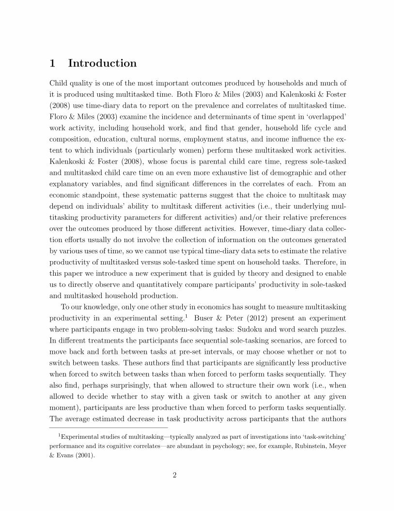
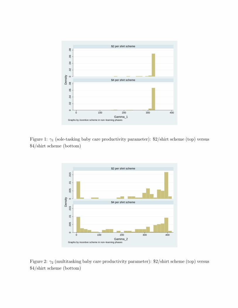
different productivity parameters are displayed in Figures 1 (γ1), 2 (γ2), 3 (z1) and 4 (z2),

separately by payoff regime.

The empirical ceiling clearly evident in Figure 1 indicates that our sole-tasked baby-

care productivity parameter is likely to be an underestimate for many participants, as the

vast majority of people performed perfectly on the baby task by keeping the baby in the

10

Table 1a: Full Covariate Definitions: Economic and Standard Demographic VariablesVariable Name Full Definition (‘pt’ stands for ‘participant’)

female 1 if pt is female; 0 otherwise

c othasian 1 if pt identifies most strongly with culture of Hong Kong, Malaysia, or Singapore;

0 otherwise

c panasian 1 if pt identifies most strongly with culture of Brunei, India, Indonesia, Japan, Pakistan, Korea, Taiwan, Vietnam,

non-specific ”Asia”, or ”eastern culture”; 0 otherwise

married 1 if pt is married; 0 otherwise

age Chronological age of pt

inc1 1 if pt reports his personal weekly after-tax income to be $100-$199;

0 otherwise

inc2 1 if pt reports his personal weekly after-tax income to be $200-$299;

0 otherwise

inc3 1 if pt reports his personal weekly after-tax income to be $300-$399;

0 otherwise

inc4 1 if pt reports his personal weekly after-tax income to be $400-$499;

0 otherwise

inc5 1 if pt reports his personal weekly after-tax income to be $500 or more;

0 otherwise

famwealth2 1 if pt reports his family to be ‘the same’ in terms of wealth as others;

0 otherwise

famwealth3 1 if pt reports his family to be ‘poorer’ than others;

0 otherwise

mumocc1 1 if pt’s mother is a manager;

0 otherwise

mumocc2 1 if pt’s mother is a professional;

0 otherwise

mumocc3 1 if pt’s mother is an associate professional;

0 otherwise

mumocc4 1 if pt’s mother is a tradesperson, transport worker or laborer;

0 otherwise

mumocc5 1 if pt’s mother is some type of clerical worker;

0 otherwise

dadocc1 1 if pt’s father is a manager;

0 otherwise

dadocc2 1 if pt’s father is a professional or associate professional;

0 otherwise

dadocc3 1 if pt’s father is a tradesperson, transport worker or laborer;

0 otherwise

dadocc4 1 if pt’s father is some type of clerical worker;

0 otherwise

mumschool1 1 if pt’s mother received no post-high school degree, or if pt does not know

his mother’s educational status; 0 otherwise

mumschool2 1 if pt’s mother received a post-high school qualification from a technical institute;

0 otherwise

mumschool3 1 if pt’s mother received a post-high school qualification from a university;

0 otherwise

dadschool1 1 if pt’s father received no post-high school degree, or if pt does not know

his father’s educational status; 0 otherwise

dadschool2 1 if pt’s father received a post-high school qualification from a technical institute;

0 otherwise

dadschool3 1 if pt’s father received a post-high school qualification from a university;

0 otherwise

Table 1b: Full Covariate Definitions: Other VariablesVariable Name Full Definition (‘pt’ stands for ‘participant’)

commerce d 1 if pt is enrolled in a Commerce degree; 0 otherwise

enjoy 1 if pt chooses value 1 through 4 on a 1 (strongly agree) to 10 (strongly disagree) scale when prompted by

‘I enjoy being busy’

goodmt 1 if pt chooses value 1 through 4 on a 1 (strongly agree) to 10 (strongly disagree) scale when prompted by

‘I think I’m good at multi-tasking’

game 1 if pt reports playing computer games or video games always, often, or sometimes;

0 if pt reports rarely or never playing such games

solebetter 1 if pt chooses value 1 through 4 on a 1 (strongly agree) to 10 (strongly disagree) scale when prompted by

‘Things get done better when you focus on doing only one thing at a time, without getting distracted’

dollplay 1 if pt reports playing caretaking games as a child always, often, or sometimes;

0 if pt reports rarely or never playing such games

siblings Number of siblings with whom pt grew up: values 0 = no siblings;

1 = 1 sibling; 2 = 2 siblings; 3 = 3 siblings; 4 = 4 or more siblings

boredeasy 1 if pt chooses value 1 through 4 on a 1 (strongly agree) to 10 (strongly disagree) scale when prompted by

‘I get bored easily’

sparetime 1 if pt reports having spare time he doesn’t know what to do with always, often, or sometimes;

0 if pt reports rarely or never having such time

freqmult 1 if pt reports doing more than one thing at home always, often, or sometimes;

0 if pt reports rarely or never having this occur

stresscc 1 if pt reports 5 or more on a scale of 0 to 10 in response to

‘How stressful did you find the sole-tasking baby care stage of the experiment?’

stresshw 1 if pt reports 5 or more on a scale of 0 to 10 in response to

‘How stressful did you find the sole-tasking clothes-sorting stages of the experiment?’

stressmult 1 if pt reports 5 or more on a scale of 0 to 10 in response to

‘How stressful did you find the multi-tasking stages of the experiment?’

political Number on a scale of 0 (very left-wing) to 10 (very right-wing) that pt chooses to represent

his political stance

hrswithkid2 1 if number of hours since age 14 pt spent awake in pt’s home in the presence of an infant under 1 year old

is 1-10; 0 otherwise

hrswithkid3 1 if number of hours since age 14 pt spent awake in pt’s home in the presence of an infant under 1 year old

is 10-100; 0 otherwise

hrswithkid4 1 if number of hours since age 14 pt spent awake in pt’s home in the presence of an infant under 1 year old

is 100 or more; 0 otherwise

hrsresponsible2 1 if number of hours pt has been completely personally responsible for the care of an infant under 1 year old

is 1-10; 0 otherwise

hrsresponsible3 1 if number of hours pt has been completely personally responsible for the care of an infant under 1 year old

is 10-100; 0 otherwise

hrsresponsible4 1 if number of hours pt has been completely personally responsible for the care of an infant under 1 year old

is 100 or more; 0 otherwise

self esteem Sum of responses, reverse-coded where necessary, on 10-item Rosenberg (Rosenberg 1965) self-esteem battery

loc full Sum of responses, reverse-coded where necessary, on 7-item Rotter (Rotter 1966) locus of control battery

happy3 1 if pt chooses ‘3’ on a scale of 1 (very unhappy) to 5 (very happy) to answer

how happy he is usually; 0 otherwise

happy4 1 if pt chooses ‘4’ on a scale of 1 (very unhappy) to 5 (very happy) to answer

how happy he is usually; 0 otherwise

happy5 1 if pt chooses ‘5’ on a scale of 1 (very unhappy) to 5 (very happy) to answer

how happy he is usually; 0 otherwise

perfuni1 1 if pt reports his performance at university to be ‘well above average’;

0 otherwise

perfuni2 1 if pt reports his performance at university to be ‘a little above average’;

0 otherwise

perfuni3 1 if pt reports his performance at university to be ‘average’;

0 otherwise

lefthand 1 if pt is left-handed; 0 otherwise

experiment 1 if pt had ever participated in an experiment before; 0 otherwise

0.0

2.0

4.0

6.0

80

.02

.04

.06

.08

0 100 200 300 400

$2 per shirt scheme

$4 per shirt scheme

Den

sity

Gamma_1Graphs by incentive scheme in non−learning phases

Figure 1: γ1 (sole-tasking baby care productivity parameter): $2/shirt scheme (top) versus

$4/shirt scheme (bottom)

0.0

05.0

1.0

150

.005

.01

.015

0 100 200 300 400

$2 per shirt scheme

$4 per shirt scheme

Den

sity

Gamma_2Graphs by incentive scheme in non−learning phases

Figure 2: γ2 (multitasking baby care productivity parameter): $2/shirt scheme (top) versus

$4/shirt scheme (bottom)

0.0

1.0

2.0

30

.01

.02

.03

0 100 200 300 400

$2 per shirt scheme

$4 per shirt scheme

Den

sity

Z_1Graphs by incentive scheme in non−learning phases

Figure 3: z1 (sole-tasking clothes-sorting productivity parameter): $2/shirt scheme (top)

versus $4/shirt scheme (bottom)

0.0

05.0

1.0

150

.005

.01

.015

0 100 200 300 400

$2 per shirt scheme

$4 per shirt scheme

Den

sity

Z_2Graphs by incentive scheme in non−learning phases

Figure 4: z2 (multitasking clothes-sorting productivity parameter): $2/shirt scheme (top)

versus $4/shirt scheme (bottom)

happiest possible mood for the entire three minutes of sole-tasked baby-care time. Baby-

care productivity fell and became far more heterogeneous across people in the multitasked

stages, as seen by comparing Figure 1 with Figure 2. Comparing the top and bottom

panels of Figure 2 also reveals more density in the left-hand side of the bottom panel than

the left-hand side of the top panel, underscoring that there was, on average, an additional

loss in baby care productivity when the alternative task of sorting shirts was more highly

remunerated. However, some participants still returned very high baby-care productivity

in the multitasked setting, even when the alternative task was more highly rewarded.

Figure 3 shows that participants’ productivity in sole-tasked clothes-sorting is not

strongly affected by the payoff regime. The loss in productivity when participants move to

a multitasked setting is shown clearly by comparing Figure 3 to Figure 4. Comparing the

top and bottom panels of Figure 4 also shows that the density of individual clothes-sorting

productivity parameters is shifted slightly rightward when the multitasking is performed

in a setting in which clothes-sorting is more highly remunerated, following participants’

material incentives.

Taken together, these figures indicate first that participants’ multitasking productivity

in each task is generally lower than their sole-tasking productivity in that task, and second

that multitasking productivity in each task is affected by the incentives embedded in the

relative payoffs available to the two tasks.

Table 2 shows descriptive statistics for the calculated productivity parameters. Note

that the productivity parameters cannot be directly compared across the two tasks, given

that the scale of the baby care productivity figures reflects the fact that baby care ‘output’

is calculated in terms of experimental dollars, whereas clothes-sorting output is calculated

in terms of numbers of shirts sorted.

Panel A presents the parameters estimated under the $2 per shirt incentive scheme,

and Panel B presents the parameters estimated under the $4 per shirt incentive scheme. In

Panel A, therefore, baby care is relatively more remunerative than clothes sorting, whereas

in Panel B, sorting clothes is relatively more remunerative than baby care. Note that neither

of the sole-task productivity parameters (γ1 or z1) changes very much across incentive

schemes. This is to be expected, given that in the sole-task settings there are no competing

tasks. However, the multitasking productivity parameters, γ2 and z2, do change as expected

across incentive schemes. When sorting clothes becomes more remunerative relative to

baby care, the measured multitasked productivity of baby care falls 15%, from 279 to

237, whereas the multitasked productivity of sorting clothes increases by 17%, from 102 to

119. Similarly, the ratio of multitasking productivity to sole-tasking productivity for baby

15

care falls from 0.86 to 0.75 as baby care becomes relatively less remunerative, while the

analogous ratio for clothes sorting increases from 0.68 to 0.77.

Table 2: Productivity Parameters

Panel A: $2 per shirt scheme

Variable N Average Std Dev Min Max

γ1 (ST baby care) 86 323.2355 23.02494 169.3045 329.5066

γ2 (MT baby care) 86 278.919 143.5545 11.44127 402.9559

z1 (ST clothes-sorting) 86 150.0413 21.50526 95.57512 193.881

z2 (MT clothes-sorting) 86 102.4068 60.71167 3.348664 261.1958

γ2/γ1 86 .8646426 .4477164 .0347224 1.811422

z2/z1 86 .6759137 .3838211 .0238889 1.580191

Panel B: $4 per shirt scheme

Variable N Average Std Dev Min Max

γ1 (ST baby care) 121 320.8518 29.29559 155.1958 329.5066

γ2 (MT baby care) 121 236.5559 149.5199 11.44127 402.9559

z1 (ST clothes-sorting) 121 151.9723 22.5721 91.93416 210.2653

z2 (MT clothes-sorting) 121 118.7761 62.83237 18.97576 276.8229

γ2/γ1 121 .7505607 .4963329 .0347224 2.248755

z2/z1 121 .7712011 .3696928 .1248324 1.635059

Data from the participants in the final three experimental rounds is used to construct

Panel A; data from participants in the pilot plus the first four experimental rounds is

used to construct Panel B. Samples exclude a handful of records which demonstrated

clear confusion about the task instructions (e.g., those earning zero dollars for any

task). See text for full descriptions of experimental treatments.

5.2 Observable correlates of the productivity parameters

In Tables 3a and 3b, we explore the extent to which the productivity parameters discussed

in the previous section are predictable using the demographic, psychological, and experien-

tial variables that we observe. Due to the plethora of covariates, we split the presentation

of these regression results into two tables. Table 3a shows coefficient estimates on the ‘eco-

nomic’ variables (such as income, family wealth, and parental background) and standard

demographic variables (such as age and gender) that we use to predict each productivity

parameter. Table 3b then shows coefficient estimates on the other variables we are able

to construct using our unique survey data. Both tables show fit statistics and observa-

16

tion counts, but each column of Table 3b is merely a continuation of the same regression

results reported in that same column from Table 3a. Columns (1) and (2) of each table

provide regressions of the productivity parameter γ1 under the $2 per shirt and $4 per shirt

schemes, respectively. Columns (3) and (4) then present regressions for γ2 under the two

incentive schemes. Columns (5) through (8) similarly provide results for z1 and z2. All

variable names in Tables 3a and 3b are explained in Tables 1a and 1b, respectively.

The most noticeable aspect of Tables 3a and 3b is a striking change in explanatory power

across columns, including even negative adjusted R-squared values in several columns de-

spite the inclusion of a host of control variables. Of course, only a modest amount of

explanatory power should be expected when the dependent variable is sole-tasking pro-

ductivity in the production of the child good (i.e., Columns (1) and (2)), given that many

individuals in the sample kept the baby completely happy for the entire duration of the

sole-tasking stage. When we move to Column (3), predicting the multitasking baby-care

productivity factor at the lower per-shirt remuneration level, the explanatory power jumps

to over 50% and many independent variables become significant. Those participants who

identify with the cultures of Hong Kong, Malaysia, or Singapore; who are married; who

have mid-range personal income levels; whose families are reportedly poorer than others;

whose mothers are managers; who are not enrolled in Commerce programs; who report

high stress associated with the child care task or low stress associated with the clothes-

sorting task; who have never been personally responsible for the care of a child; or who

report themselves to be well above-average students have statistically significantly higher

multitasking child care productivities at a 5% or lower p-value than other participants.

This increase would most logically be offset by a lower productivity in the clothes-sorting

activity. Indeed, when we predict multitasking housework productivity in the $2 per shirt

scheme in Column (7), that is just what we see for many of the same covariates. This

compensating effect is evident for marital status, income, wealth, program of study, and

stress associated with the child care task. For all other variables significant in Column

(3), the compensating effects presented in Column (7) are in the correct direction but do

not achieve statistical significance at the 5% level. We also note that many other vari-

ables’ coefficient estimates in both columns are very large in magnitude but do not achieve

statistical significance, probably due to modest sample size.

Our primary interpretation of the results in Columns (3) and (7) is that certain types

of economic and cultural backgrounds predispose a person to spend more effort on the

interactive baby-care task than on the menial clothes-sorting task when faced with the

multitasking context and the lower payoff to clothes-sorting. Some people may simply be

17

raised to place a particularly high value on the child good relative to the household good.

Even in a setting in which the household good is almost as valuable in monetary terms as

the child good, these people still follow their habits and spend more effort than others do

on the baby, and less effort than others do on the household task.

The most interesting results in Tables 3a and 3b relate to how the strength and sig-

nificance of the explanatory variables change as we change incentive schemes in the multi-

tasking context. Specifically, paying more per shirt in the multitasking setting (Columns

(8) and (4) compared to Columns (7) and (3), respectively) appears to wipe out both ex-

planatory power and statistically significant relationships, almost across the board. This

suggests that apparent multitasking productivity differentials—which may arise through

upbringing, genes, or habit—can be overcome with a change in economic incentives.

Sole-tasking productivity in the production of the household good (Columns (5) and

(6)) is fairly well-predicted, though not as well as multitasking productivities in the $2

per shirt scheme. z1 is negatively associated with mid-range parental wealth, having a

mother who works in a clerical occupation, having a mother with a university degree, and

frequently feeling rushed. It could be that such individuals’ more-advantaged upbringing

may make it less necessary for them to acquire household production skills, or may lead

them to place a lower absolute value on performing menial household-production tasks.

In Tables 4a and 4b, the ratios of productivity factors, γ2/γ1 and z2/z1, are the depen-

dent variables, and the table structure is identical to that of Tables 3a and 3b. Under the

$2 per shirt incentive scheme, statistically significantly higher relative productivity of mul-

titasked time in the production of the child good is coupled with statistically significantly

lower relative productivity of multitasked time in the production of the household good for

the those who identify with the cultures of Hong Kong, Malaysia, or Singapore; who are

married; who have mid-range personal income levels; whose families are reportedly poorer

than others; or who report high stress associated with the child care task. These results

are consistent with the results in Tables 3a and 3b, and the other variables significant in

those prior tables do show the expected signs in Tables 4a and 4b, though without sta-

tistical significance at the 5% level. Also consistent with our prior results, changing the

payoff to $4 per shirt removes all of these correlations and sends the explanatory power

of the regressions into the negative range, suggesting that innate preferences for the child

good in a multitasking context can be overcome with an increase in the relative payoff to

housework.

18

Table 3a: Correlates of Productivity Parameters: Economic and Standard Demographic

Covariates(1) (2) (3) (4) (5) (6) (7) (8)

— γ1 — — γ2 — — z1 — — z2 —

Scheme $2 per shirt $4 per shirt $2 per shirt $4 per shirt $2 per shirt $4 per shirt $2 per shirt $4 per shirt

female -0.282 -9.411 -62.947 -13.242 7.449 -2.180 15.260 -8.289

(22.14) (6.56) (83.40) (55.16) (15.54) (6.28) (40.37) (22.42)

c othasian 39.530 3.787 390.993* 173.449* 41.437 1.301 -127.592 -49.743

(39.45) (8.75) (148.59) (73.50) (27.68) (8.37) (71.92) (29.87)

c panasian 21.919 -2.706 244.908 31.256 -17.431 -11.696 -60.754 -29.024

(33.11) (9.13) (124.71) (76.77) (23.23) (8.74) (60.36) (31.20)

married 74.195 -50.635 926.628* 401.205 -41.781 -45.042 -374.532* -186.789

(80.75) (30.89) (304.18) (259.60) (56.66) (29.56) (147.23) (105.50)

age -2.324 0.894 -41.732 -1.841 2.421 3.336* 19.064 2.125

(6.14) (1.61) (23.12) (13.55) (4.31) (1.54) (11.19) (5.51)

inc1 24.572 5.647 171.837 95.740 -1.885 -4.730 -46.687 -17.474

(24.93) (10.23) (93.92) (85.98) (17.49) (9.79) (45.46) (34.94)

inc2 -12.877 -5.191 286.913* 70.338 -24.577 4.806 -126.134* -24.868

(25.51) (13.10) (96.07) (110.14) (17.90) (12.54) (46.50) (44.76)

inc3 -65.502 12.892 224.105 259.022 17.178 4.530 -57.686 -86.639

(61.65) (15.79) (232.23) (132.69) (43.26) (15.11) (112.40) (53.92)

inc4 3.019 8.320 378.576 105.253 32.637 4.534 -135.829 -22.241

(44.22) (18.09) (166.56) (152.07) (31.03) (17.32) (80.62) (61.80)

inc5 -20.782 -6.848 -238.868 -35.520 33.993 -15.250 99.298 10.549

(53.82) (13.57) (202.73) (114.08) (37.76) (12.99) (98.13) (46.36)

famwealth2 -41.786 -5.804 107.792 105.926 -13.111 -17.532* -30.307 -54.729

(29.30) (7.93) (110.38) (66.62) (20.56) (7.59) (53.43) (27.07)

famwealth3 -20.308 15.623 628.056* -22.535 14.103 17.009 -296.920* -3.485

(60.78) (14.78) (228.94) (124.20) (42.64) (14.14) (110.81) (50.48)

mumocc1 -6.223 9.705 293.923* 37.300 37.624 -2.863 -74.918 -17.933

(33.23) (10.01) (125.17) (84.14) (23.32) (9.58) (60.59) (34.19)

mumocc2 -10.150 0.191 -96.509 -13.709 -1.971 7.848 54.114 20.013

(20.05) (10.50) (75.54) (88.22) (14.07) (10.05) (36.56) (35.85)

mumocc3 -47.622 18.730 -17.632 93.773 -0.956 -5.342 11.496 -51.759

(35.96) (12.68) (135.46) (106.56) (25.23) (12.13) (65.57) (43.30)

mumocc4 -2.318 43.830* 3.544 66.575 -13.186 24.657 24.761 -12.932

(30.94) (17.93) (116.56) (150.69) (21.71) (17.16) (56.42) (61.24)

mumocc5 -32.630 10.020 -139.123 112.835 -31.176 -22.936* 54.788 -70.256*

(30.24) (9.67) (113.89) (81.27) (21.21) (9.25) (55.12) (33.03)

dadocc1 8.659 -1.547 225.625 -28.372 68.097 -9.100 -105.619 3.395

(54.14) (17.78) (203.92) (149.40) (37.98) (17.01) (98.70) (60.72)

dadocc2 -14.584 -18.363 -60.861 12.561 54.342 -17.582 6.198 -20.774

(55.04) (18.66) (207.32) (156.82) (38.62) (17.86) (100.35) (63.73)

dadocc3 41.166 -2.045 430.312 -135.350 81.581 13.913 -173.906 54.339

(54.54) (19.61) (205.43) (164.80) (38.27) (18.77) (99.43) (66.97)

dadocc4 36.873 5.460 307.908 -150.579 25.188 2.805 -135.928 48.194

(46.88) (21.86) (176.60) (183.73) (32.89) (20.92) (85.48) (74.67)

mumschool1 -6.517 -9.664 -174.365 22.162 -21.165 -6.768 77.233 -20.527

(23.75) (13.23) (89.48) (111.16) (16.67) (12.66) (43.31) (45.18)

mumschool2 2.448 9.353 70.975 0.410 -32.163 -21.587 -16.340 -20.256

(30.14) (11.19) (113.54) (94.05) (21.15) (10.71) (54.96) (38.22)

mumschool3 -21.605 -1.030 -27.896 86.766 -63.402* -4.704 -7.963 -49.210

(28.55) (10.73) (107.55) (90.18) (20.03) (10.27) (52.06) (36.65)

dadschool1 7.200 27.144 -15.346 -26.957 26.663 4.797 30.516 29.078

(37.06) (13.80) (139.58) (115.96) (26.00) (13.20) (67.56) (47.12)

dadschool2 38.002 35.750* -132.569 -133.100 0.749 38.627** 76.919 81.311

(26.15) (14.72) (98.49) (123.74) (18.34) (14.09) (47.67) (50.29)

dadschool3 -3.321 24.457* -198.502 -115.717 18.252 7.833 65.054 66.691

(31.07) (10.61) (117.02) (89.21) (21.80) (10.16) (56.64) (36.25)

AdjR-sq -0.119 0.047 0.511 -0.159 0.210 0.249 0.392 -0.114

Obs 69 98 69 98 69 98 69 98

* p < 0.05, ** p < 0.01, *** p < 0.001. See text for dependent variable definitions. Samples in

odd-numbered columns include participants in the final three experimental rounds; samples in even-

numbered columns include participants in the pilot and first four experimental rounds. Samples

sizes differ from those of Table 2 because both samples used in these regressions exclude all records

whose survey data were incomplete.

Table 3b: Correlates of Productivity Parameters: Other Covariates(1) (2) (3) (4) (5) (6) (7) (8)

— γ1 — — γ2 — — z1 — — z2 —

Scheme $2 per shirt $4 per shirt $2 per shirt $4 per shirt $2 per shirt $4 per shirt $2 per shirt $4 per shirt

commerce d 5.018 4.144 -181.545* 43.271 12.873 4.839 79.550* -4.152

(18.90) (7.66) (71.20) (64.37) (13.26) (7.33) (34.46) (26.16)

enjoy 5.154 4.264 81.215 55.010 -24.268 12.211 -30.852 -26.363

(22.00) (9.07) (82.88) (76.20) (15.44) (8.68) (40.12) (30.97)

goodmt -18.566 -13.371 92.789 9.787 -11.272 -1.852 -19.793 11.067

(24.41) (8.71) (91.93) (73.23) (17.12) (8.34) (44.50) (29.76)

game 18.721 17.719* 22.541 25.001 -34.874 11.409 8.274 5.227

(30.21) (7.46) (113.78) (62.67) (21.19) (7.14) (55.07) (25.47)

solebetter 13.487 -0.851 -205.699 15.983 0.734 0.795 39.719 1.606

(31.88) (11.49) (120.08) (96.57) (22.37) (11.00) (58.12) (39.24)

dollplay -2.398 0.022 46.589 -38.781 -22.555 1.092 -18.537 15.166

(16.49) (6.17) (62.13) (51.87) (11.57) (5.91) (30.07) (21.08)

siblings 19.373 0.875 36.189 -8.630 -5.507 2.466 -15.209 2.907

(11.57) (2.32) (43.59) (19.46) (8.12) (2.22) (21.10) (7.91)

boredeasy -6.718 9.426 167.942 42.951 0.785 0.669 -59.731 -13.198

(19.42) (7.43) (73.14) (62.42) (13.62) (7.11) (35.40) (25.37)

sparetime -54.125 0.170 61.484 28.860 6.661 -2.311 -29.806 -6.501

(26.27) (6.98) (98.93) (58.66) (18.43) (6.68) (47.89) (23.84)

freqmult 13.429 18.761 608.609 478.024 -66.105 -10.416 -167.230 -169.444

(168.61) (32.13) (635.10) (270.03) (118.30) (30.75) (307.40) (109.74)

feelsrushed 9.134 -32.843 79.118 237.047 -9.316 -49.161** -25.915 -143.384*

(38.37) (18.20) (144.54) (152.95) (26.92) (17.42) (69.96) (62.16)

stresscc 8.385 -15.415* 325.085** 15.859 5.486 13.309 -108.391* 8.404

(21.69) (7.44) (81.71) (62.51) (15.22) (7.12) (39.55) (25.40)

stresshw -18.272 8.072 -211.053* 1.254 12.033 -14.069 58.109 -5.987

(20.47) (7.88) (77.12) (66.25) (14.36) (7.54) (37.33) (26.93)

stressmult -13.695 -1.228 156.632 -48.040 7.008 -4.382 -47.510 -1.858

(20.98) (9.37) (79.03) (78.75) (14.72) (8.97) (38.25) (32.00)

political -0.929 0.118 -4.566 -7.310 -2.143 0.778 -2.705 -0.877

(4.54) (1.82) (17.08) (15.32) (3.18) (1.74) (8.27) (6.23)

hrswithkid2 -38.725 -20.012 18.347 50.199 -46.523* 8.176 -11.975 -15.581

(26.22) (11.59) (98.76) (97.40) (18.40) (11.09) (47.80) (39.58)

hrswithkid3 -87.110 -4.303 129.900 -56.399 22.377 7.667 -64.575 24.883

(65.59) (9.47) (247.06) (79.59) (46.02) (9.06) (119.58) (32.34)

hrswithkid4 -20.956 -0.805 45.059 -32.250 7.353 -13.885 -2.940 7.671

(42.87) (12.75) (161.49) (107.18) (30.08) (12.20) (78.17) (43.56)

hrsresponsible2 22.904 -2.850 -65.494 22.086 22.509 -29.108** 14.912 -32.242

(32.16) (10.26) (121.15) (86.24) (22.57) (9.82) (58.64) (35.05)

hrsresponsible3 -1.973 13.161 -521.966* 69.661 11.377 2.959 163.593 -14.750

(48.80) (10.38) (183.81) (87.26) (34.24) (9.94) (88.97) (35.46)

hrsresponsible4 3.390 -37.168 -43.453 221.498 51.794 -40.909 -37.703 -119.491

(60.27) (23.83) (227.00) (200.26) (42.28) (22.80) (109.88) (81.38)

self esteem -4.663 -1.041 -9.377 -22.586 -4.435 5.089 7.801 14.306

(8.53) (3.39) (32.14) (28.48) (5.99) (3.24) (15.56) (11.58)

loc full -0.401 1.014* 3.647 -1.421 0.805 -0.169 -2.094 0.057

(1.13) (0.44) (4.27) (3.69) (0.80) (0.42) (2.07) (1.50)

happy3 -69.381 40.963 687.427 136.946 -19.740 43.641 -269.002 -41.805

(94.21) (37.25) (354.86) (313.10) (66.10) (35.65) (171.76) (127.24)

happy4 -29.695 40.252 577.822 239.435 -21.788 20.979 -222.362 -97.572

(82.83) (37.27) (311.98) (313.27) (58.11) (35.67) (151.01) (127.31)

happy5 21.243 36.200 485.050 269.131 -44.329 25.224 -212.847 -96.621

(67.83) (39.28) (255.50) (330.13) (47.59) (37.59) (123.67) (134.16)

perfuni1 55.102 -0.516 868.048* 68.392 -13.315 2.803 -264.213 -13.395

(72.59) (17.52) (273.44) (147.28) (50.93) (16.77) (132.35) (59.86)

perfuni2 -24.508 -2.383 373.905 128.846 -25.183 4.158 -75.687 -34.701

(70.93) (15.33) (267.18) (128.84) (49.77) (14.67) (129.32) (52.36)

perfuni3 14.449 -6.231 430.269 35.291 -21.088 25.210 -106.817 12.364

(63.65) (15.96) (239.76) (134.12) (44.66) (15.27) (116.05) (54.51)

lefthand -63.339 -0.747 3.208 26.634 -71.065 -17.477 32.984 -24.190

(72.52) (13.18) (273.17) (110.77) (50.88) (12.61) (132.22) (45.02)

experiment -70.483 0.388 -144.592 33.636 31.179 -1.397 33.070 -15.524

(43.31) (8.34) (163.12) (70.13) (30.38) (7.99) (78.95) (28.50)

AdjR-sq -0.119 0.047 0.511 -0.159 0.210 0.249 0.392 -0.114

Obs 69 98 69 98 69 98 69 98

* p < 0.05, ** p < 0.01, *** p < 0.001. See text for dependent variable definitions. Samples in

odd-numbered columns include participants in the final three experimental rounds; samples in even-

numbered columns include participants in the pilot and first four experimental rounds. Samples

sizes differ from those of Table 2 because both samples used in these regressions exclude all records

whose survey data were incomplete. This table is a continuation of Table 3a.

Table 4a: Correlates of Relative Productivity of Multitasking to Sole-tasking: Economic

and Standard Demographic Covariates(1) (2) (3) (4)

— γ2/γ1 — — z2/z1 —

Scheme $2 per shirt $4 per shirt $2 per shirt $4 per shirt

female -0.138 0.009 0.012 -0.083

(0.25) (0.18) (0.25) (0.13)

c othasian 1.173* 0.503* -1.034* -0.337

(0.45) (0.24) (0.44) (0.18)

c panasian 0.642 0.106 -0.233 -0.138

(0.37) (0.25) (0.37) (0.18)

married 2.520* 1.456 -2.103* -1.023

(0.91) (0.85) (0.90) (0.62)

age -0.125 -0.006 0.129 0.003

(0.07) (0.04) (0.07) (0.03)

inc1 0.411 0.275 -0.306 -0.078

(0.28) (0.28) (0.28) (0.21)

inc2 0.987** 0.214 -0.722* -0.170

(0.29) (0.36) (0.28) (0.26)

inc3 0.935 0.685 -0.360 -0.617

(0.70) (0.43) (0.69) (0.32)

inc4 1.200* 0.273 -1.079 -0.244

(0.50) (0.50) (0.49) (0.36)

inc5 -0.646 -0.067 0.382 0.124

(0.61) (0.37) (0.60) (0.27)

famwealth2 0.455 0.348 -0.049 -0.247

(0.33) (0.22) (0.33) (0.16)

famwealth3 2.031* -0.161 -1.937* -0.131

(0.69) (0.41) (0.68) (0.30)

mumocc1 1.000* 0.035 -0.574 -0.105

(0.38) (0.27) (0.37) (0.20)

mumocc2 -0.235 -0.043 0.445 0.082

(0.23) (0.29) (0.22) (0.21)

mumocc3 -0.013 0.173 0.211 -0.287

(0.41) (0.35) (0.40) (0.26)

mumocc4 -0.068 -0.036 0.314 -0.155

(0.35) (0.49) (0.34) (0.36)

mumocc5 -0.388 0.252 0.629 -0.308

(0.34) (0.27) (0.34) (0.19)

dadocc1 0.809 -0.108 -1.177 0.077

(0.61) (0.49) (0.60) (0.36)

dadocc2 -0.108 0.107 -0.346 -0.061

(0.62) (0.51) (0.61) (0.38)

dadocc3 1.313 -0.402 -1.666* 0.283

(0.62) (0.54) (0.61) (0.39)

dadocc4 0.896 -0.534 -1.068 0.314

(0.53) (0.60) (0.52) (0.44)

mumschool1 -0.578 0.120 0.704* -0.120

(0.27) (0.36) (0.26) (0.27)

mumschool2 0.120 -0.076 0.165 -0.018

(0.34) (0.31) (0.34) (0.23)

mumschool3 -0.094 0.279 0.323 -0.305

(0.32) (0.29) (0.32) (0.22)

dadschool1 -0.003 -0.215 -0.005 0.184

(0.42) (0.38) (0.41) (0.28)

dadschool2 -0.543 -0.607 0.474 0.366

(0.30) (0.40) (0.29) (0.30)

dadschool3 -0.573 -0.483 0.225 0.418

(0.35) (0.29) (0.35) (0.21)

AdjR-sq 0.550 -0.181 0.444 -0.095

Obs 69 98 69 98

* p < 0.05, ** p < 0.01, *** p < 0.001. Sample selection

is identical to that applied to create Tables 3a and 3b.

Table 4b: Correlates of Relative Productivity of Multitasking to Sole-tasking: Other Co-

variates(1) (2) (3) (4)

— γ2/γ1 — — z2/z1 —

Scheme $2 per shirt $4 per shirt $2 per shirt $4 per shirt

commerce d -0.572* 0.112 0.436 -0.068

(0.21) (0.21) (0.21) (0.15)

enjoy 0.130 0.124 -0.091 -0.259

(0.25) (0.25) (0.24) (0.18)

goodmt 0.360 0.127 0.011 0.061

(0.28) (0.24) (0.27) (0.18)

game -0.134 -0.044 0.243 -0.040

(0.34) (0.20) (0.34) (0.15)

solebetter -0.557 0.028 0.099 0.013

(0.36) (0.31) (0.35) (0.23)

dollplay 0.024 -0.119 0.062 0.076

(0.19) (0.17) (0.18) (0.12)

siblings 0.022 -0.029 -0.067 0.002

(0.13) (0.06) (0.13) (0.05)

boredeasy 0.562* 0.068 -0.321 -0.091

(0.22) (0.20) (0.22) (0.15)

sparetime 0.454 0.093 -0.199 0.003

(0.30) (0.19) (0.29) (0.14)

freqmult 1.491 1.359 -0.132 -1.041

(1.91) (0.88) (1.88) (0.65)

feelsrushed 0.260 0.857 -0.132 -0.719

(0.43) (0.50) (0.43) (0.37)

stresscc 0.962** 0.144 -0.616* -0.018

(0.25) (0.20) (0.24) (0.15)

stresshw -0.530 -0.046 0.281 0.080

(0.23) (0.22) (0.23) (0.16)

stressmult 0.607* -0.154 -0.368 -0.004

(0.24) (0.26) (0.23) (0.19)

political 0.003 -0.025 -0.025 -0.008

(0.05) (0.05) (0.05) (0.04)

hrswithkid2 0.084 0.283 0.195 -0.128

(0.30) (0.32) (0.29) (0.23)

hrswithkid3 0.766 -0.157 -0.389 0.179

(0.74) (0.26) (0.73) (0.19)

hrswithkid4 0.174 -0.094 0.008 0.195

(0.48) (0.35) (0.48) (0.26)

hrsresponsible2 -0.181 0.062 -0.118 -0.072

(0.36) (0.28) (0.36) (0.21)

hrsresponsible3 -1.475* 0.152 0.804 -0.147

(0.55) (0.28) (0.54) (0.21)

hrsresponsible4 0.251 0.868 -0.622 -0.612

(0.68) (0.65) (0.67) (0.48)

self esteem -0.052 -0.050 0.106 0.062

(0.10) (0.09) (0.09) (0.07)

loc full 0.018 -0.012 -0.020 0.000

(0.01) (0.01) (0.01) (0.01)

happy3 2.174 0.078 -1.184 -0.630

(1.06) (1.02) (1.05) (0.75)

happy4 1.726 0.388 -0.926 -0.845

(0.94) (1.02) (0.92) (0.75)

happy5 1.277 0.481 -0.915 -0.830

(0.77) (1.08) (0.75) (0.79)

perfuni1 2.290* 0.202 -1.405 -0.152

(0.82) (0.48) (0.81) (0.35)

perfuni2 0.933 0.437 -0.055 -0.269

(0.80) (0.42) (0.79) (0.31)

perfuni3 0.976 0.190 -0.331 -0.066

(0.72) (0.44) (0.71) (0.32)

lefthand -0.157 0.085 0.829 -0.083

(0.82) (0.36) (0.81) (0.27)

experiment -0.101 0.090 0.071 -0.092

(0.49) (0.23) (0.48) (0.17)

AdjR-sq 0.550 -0.181 0.444 -0.095

Obs 69 98 69 98

* p < 0.05, ** p < 0.01, *** p < 0.001. Sample selection is

identical to that applied to create Tables 3a and 3b. This

table is a continuation of Table 4a

5.3 Productivity responses to multitasking and incentives

We now proceed to estimating average task-specific productivity losses due to multitasking,

together with the own- and cross- price elasticities of task performance.

5.3.1 Which is better: Sequential sole-tasking, or multitasking?

We first use our results on productivity to ask the following question, for each participant: If

a window of time were available in which s/he could either sequentially sole-task (spending

half the time in each task) or multitask for the entire time, which would be better for

him/her to choose, purely from a productivity standpoint?

Figure 5 provides the graphical answer to this question, where the analysis is conducted

separately by incentive scheme. The left-hand graph shows results for the $2-per-shirt

incentive scheme, and the right-hand graph shows results for the $4-per-shirt incentive

scheme. The vertical axis is the percentage of participants for whom a particular result

applies, where the denominator of this percentage is the total number of participants who

faced the given compensation scheme during their ‘non-learning’ phases.

Our results indicate that, for the vast majority of people, multitasking is preferable

for at least one task in terms of the total output produced. Sequential sole-tasking is

almost never preferable–except for a very small number of participants in the $2-per-shirt

incentive scheme. We also see that the change to a higher relative payoff for housework

induces a change in the distribution of optimal time allocations for the two tasks, in the

expected direction. Specifically, the largest group of participants in the low-payoff regime

would generate higher baby care productivity under the multitasking allocation and higher

housework productivity under the sequential sole-tasking regime. Once we pay more per

shirt, the gap narrows between this group of participants and the next-highest group,

for whom sequential sole-tasking is preferable from a baby-care productivity standpoint,

but multitasking is preferable from a housework standpoint. Essentially, this group size

shift illustrates the exertion of more effort to increase the multitasking productivity of

housework, in order to capitalize on the increased economic incentives for shirts correctly

sorted, and less effort on the baby care task.

5.3.2 Elasticities

Finally, we move to a calculation of aggregate elasticity figures. To obtain these figures,

we first calculate average products for each use of time for each good under each payoff

regime and stage-order structure. As before, a participant’s total productivity in a baby-

23

0.2

.4.6

Per

cent

of p

artic

ipan

ts

$2 per shirt scheme $4 per shirt scheme

Which is More Productive: Sequential Sole−tasking, or Multitasking?

ST Better ST Better for Baby Care,MT Better for Housework

MT Better for Baby Care,ST Better for Housework MT Better

Figure 5: $2/shirt scheme (left) versus $4/shirt scheme (right)

care task is calculated as the total money payoff the participant earned in that task. To

construct the participant’s average product per minute, we divide this figure by the number

of minutes spent in the stage in which that payoff was earned for that task (three minutes

if sole-tasked and six minutes if multitasked). Average product in the clothes-sorting task

is calculated as the number of shirts sorted correctly minus the number of shirts sorted

incorrectly, divided by the number of minutes spent in the stage in which that task was

undertaken.

Panel A of Table 5 shows average products in the sole-tasking stages for the baby-care

and clothes-sorting tasks, for each payoff regime and stage-order structure. Panel B of

Table 5 shows similar figures for the multitasking stages. All figures represent means and

standard deviations across the entire cell of experimental participants. Bolded figures in

Table 5 represent those means that are plausibly uncontaminated by any learning effects,

as they are calculated using only the second instances of the clothes-sorting task. Only

these figures are used in calculating the relative productivity measures discussed below.6

The figures in Table 5 imply that the loss in baby-care average product due to moving

6The magnitude of the learning effect, calculated by comparing mean average product in the first sole-

tasked clothes-sorting task that participants faced to the second one (roughly 47 and 55 respectively, as

shown in Table 5), is roughly 8 shirts per minute. Again, it is evident that there are no learning effects for

baby care.

24

from a sole-tasked to multitasked environment is between 29% and 40%, depending on the

level of remuneration offered in the clothes-sorting task that competed for the participant’s

effort in the multitasking stage.7 Not surprisingly, the more valuable the alternative task

(sorting clothes) was to participants, the more that average per-minute product in the

baby-care task fell in moving from the sole-tasked to the multitasked environment.

For sorting clothes, the figures in Table 5 imply that moving from a sole-tasking to a

multitasking environment results in a loss in average product of between 36% and 46%,

again depending upon the relative remuneration available in the two tasks competing for

participants’ effort in the multitasking context.

These average product losses are far greater than those found by Buser & Peter (2012).

However, in addition to the fact that our study investigates very different tasks than theirs,

our design features bona fide multitasking: participants face two tasks that are simulta-

neously competing for their attention, while the design of Buser & Peter (2012) presents

tasks in sequence but with different (enforced versus optional) switching regimes.

Using the numbers in Table 5, we can compute rough estimates of the relevant own- and

cross-price elasticities of task supply for baby care and sorting clothes. When we double

the opportunity cost of baby care, by moving from the low-payoff regime to the high-payoff

regime, baby-care average product in the multitasked setting decreases by 16.84%, whereas

average product in the clothes-sorting task increases by 19.71%. The first of these figures

translates into an own-price output elasticity of -0.1685 for the baby care task within

the multitasking setting, while the second translates into a cross-price output elasticity of

0.1971.

In the opposite direction, moving from the $4 per shirt scheme to the $2 per shirt

scheme doubles the opportunity cost of sorting clothes. This change then brings about a

decrease in the clothes-sorting average product of 16.46%, with a concomitant increase in

baby-care average product of 20.25%. Hence, the own-price supply elasticity for clothes-

sorting is roughly -.1646, very similar to that of baby care. The estimate of the cross-price

supply elasticity of baby care is .2025, also very similar to that of clothes sorting. These

results indicate that economic incentives are clearly at work with respect to multitasking.

Participants are willing to perform less baby care in a multitasked setting if they are

7As mentioned above when discussing the histogram of baby care productivity parameters, it should be

noted that approximately 64% of participants earned the maximum amount possible in the sole-tasked baby

care stage. This may mean that the average product losses estimated in this section are underestimates.

However, re-calculating the figures above using only those participants who did not earn the maximum in

the sole-tasked baby care stage yields slightly smaller, but still fairly similar, estimated losses for the baby

care task: 23% and 32% in the low-payoff and high-payoff regimes respectively.

25

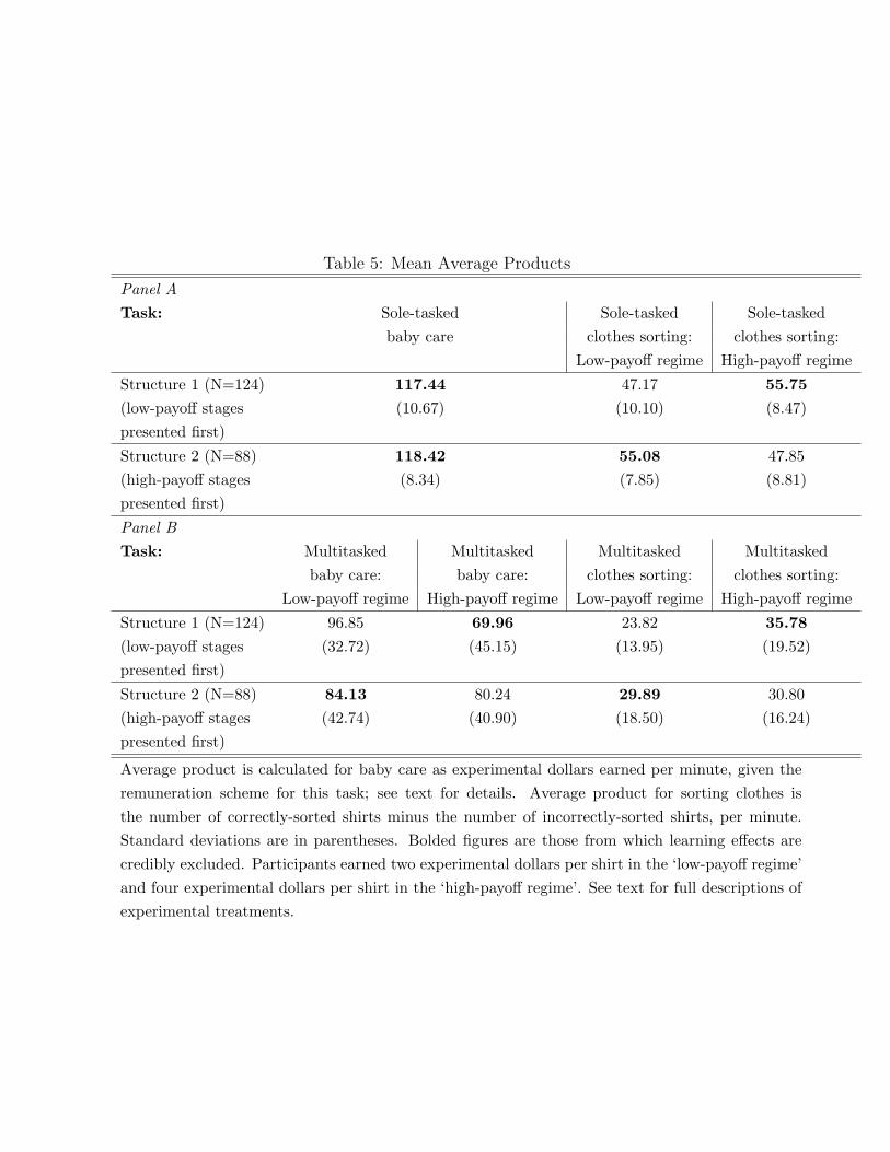
Table 5: Mean Average Products

Panel A

Task: Sole-tasked Sole-tasked Sole-tasked

baby care clothes sorting: clothes sorting:

Low-payoff regime High-payoff regime

Structure 1 (N=124) 117.44 47.17 55.75

(low-payoff stages (10.67) (10.10) (8.47)

presented first)

Structure 2 (N=88) 118.42 55.08 47.85

(high-payoff stages (8.34) (7.85) (8.81)

presented first)

Panel B

Task: Multitasked Multitasked Multitasked Multitasked

baby care: baby care: clothes sorting: clothes sorting:

Low-payoff regime High-payoff regime Low-payoff regime High-payoff regime

Structure 1 (N=124) 96.85 69.96 23.82 35.78

(low-payoff stages (32.72) (45.15) (13.95) (19.52)

presented first)

Structure 2 (N=88) 84.13 80.24 29.89 30.80

(high-payoff stages (42.74) (40.90) (18.50) (16.24)

presented first)

Average product is calculated for baby care as experimental dollars earned per minute, given the

remuneration scheme for this task; see text for details. Average product for sorting clothes is

the number of correctly-sorted shirts minus the number of incorrectly-sorted shirts, per minute.

Standard deviations are in parentheses. Bolded figures are those from which learning effects are

credibly excluded. Participants earned two experimental dollars per shirt in the ‘low-payoff regime’

and four experimental dollars per shirt in the ‘high-payoff regime’. See text for full descriptions of

experimental treatments.

compensated for it, which is accomplished in our experiment through increased pay for the

alternative task of sorting clothes.

6 Conclusion

Our paper provides the first economic estimates of the relative productivity of multitasked

time to sole-tasked time in individuals’ production of child and household goods, using

a novel experimental approach. Our results show raw output reductions associated with

multitasking that are far greater than those estimated in prior experimental work. We

believe this is due to the different tasks that we analyze and the different approach that

we take in our experimental design compared to that taken in prior work.

In our experiment we represent a change in preferences by a change in the relative

monetary payoffs of the clothes-sorting and baby-care tasks. Using this approach, we

are able to calculate own- and cross-price elasticities of supply for sorting clothes and

baby care. Our results suggest, at a minimum, the order of magnitude of a change in

multitasking performance for which differences across people in these utility parameters

may be responsible. They also suggest that the influence of preferences or habits may be

able to be meaningfully moderated through the application of targeted economic incentives.

27

7 Appendix

7.1 Questionnaire

The following questions/statements were posed to participants before the income-earning

stages of the experiment. The statements were followed by scaled answer alternatives,

ranging from Strongly Agree to Strongly Disagree, or Always to Never. Double-asterisked

items form part of the modified Rosenberg (1965) self-esteem battery; single-asterisked

items form part of the modified Rotter (1966) locus of control battery:

• I get bored easily.

• I think I’m good at multitasking.

• I enjoy being busy.

• Things get done better when you focus on doing only one thing at a time, without getting

distracted.

• On the whole, I am satisfied with myself.**

• At times I think I am no good at all.**

• I feel that I have a number of good qualities.**

• I am able to do things as well as most people.**

• I feel I do not have much to be proud of.**

• I certainly feel useless at times.**

• I feel that I am a person of worth, or at least on an equal plane with others.**

• I wish I could have more respect for myself.**

• All in all, I am inclined to feel that I am a failure.**

• I take a positive attitude toward myself.**

• How often do you feel rushed or pressed for time?

• How often do you have spare time that you don’t know what to do with?

• How often do you play computer games or video games?

• When you are at home, how often do you find yourself doing more than one thing at once?

28

• When you were a child, how often did you play caretaking games with dolls and/or stuffed

animals?

• I have little control over the things that happen to me.*

• There is really no way I can solve some of the problems I have.*

• There is little I can do to change many of the important things in my life.*

• I often feel helpless in dealing with the problems of life.*

• Sometimes I feel that I’m being pushed around in life.*

• What happens to me in the future mostly depends on me.*

• I can do just about anything I really set my mind to.*

The following questions were posed to participants after the income-earning stages of

the experiment:

• How stressful did you find the multitasking stages of the experiment?

• How stressful did you find the sole-tasking clothes-sorting stages of the experiment?

• How stressful did you find the sole-tasking baby-care stage of the experiment?

• What is your year of birth?

• What is your month and day of birth?

• Please indicate your gender.

• Please type in your nationality/citizenship.

• Please type in the country in which you were born.

• Please type in the country whose culture you identify with most strongly.

• Please type in the postcode of the area you live in.

• Please type in the name of the UNSW degree program in which you are enrolled, if any

(Bachelor of Economics; Bachelor of Commerce; Masters of Commerce; etc.).

• When do you expect to graduate (month and year)?

• Are you a UNSW student?

• Are you an international student?

29

• Have you ever participated in an experiment before?

• What is your personal weekly after-tax income from all sources?

• Do you speak English at home?

• What is your current living situation?

• Are you currently...(married, in a partnership, or single).

• Are you a parent?

• How many siblings did you grow up with (in the same household?

• How many hours in your adult life (over 14 yrs old) have you spent awake in your home in

the presence of an infant under 1 year old?

• How many hours in your life have you been completely personally responsible for the care

of an infant under 1 year old?

• How many people under age 15 are you currently living with (in the same household?

• How many women aged 15 or older are living in your household (including yourself, if

applicable)? [Only asked of participants who are living with children.]

• How many parents of children under age 15 who are living in your household also live in

your household (including yourself, if applicable)? [Only asked of participants who are

living with children.]

• How many people aged 15 or older are living in your household and are NOT parents of

children under 15 living in your household (including yourself, if applicable)? [Only asked

of participants who are living with children.]

• Please type in the age of the youngest child in your household. [Only asked of participants

who are living with children.]

• What is the highest year of school you have completed?

• How much schooling did your mother complete?

• How much schooling did your father complete?

• Did your mother complete an educational qualification after leaving school? Please include

any trade certificates, apprenticeships, diplomas, degrees or other educational qualifications.

• If yes, from where was her highest level qualification obtained?

30

• Did your father complete an educational qualification after leaving school? Please include

any trade certificates, apprenticeships, diplomas, degrees or other educational qualifications.

• If yes, from where was his highest level qualification obtained?

• Please select the category of class of professions your mother’s occupation falls into.

• Please select the category of class of professions your father’s occupation falls into.

• Which hand do you write with?

• In political matters, people talk of ”the left” and ”the right”. How would you place your

views on this scale, generally speaking?

• All things considered in your life, how happy would you say you are usually?

• Would you say that your family is ... (wealthier, the same, or poorer than others)?

• Overall, how would you rate your performance at university?

31

7.2 Hard-copy instructions to participants

Figures 6 (front) and 7 (back) are reproductions of the contents of the instruction sheet

presented to participants when they entered the ASBLab to participate in this experiment.

Participant Information Statement

(HREC 10239, valid until 18 August 2015)

Participant SelectionYou are invited to participate in the study described below. You were selected as a possible participant in this study either as part of a course in which you are enrolled, or due to your indication that you wished to be part of an experimental subject pool within the Australian School of Business, in which case you accepted an emailed invitation to participate.

Purpose of the StudyThis study investigates human behavior in the presence of incentives. The experimenters are testing theories involving incentives in order to better understand how individuals make decisions as individuals and in groups.

Description of the StudyIn this study, you will participate in one or more decision-making scenarios, or experiments. In each experiment, you will make a series of choices, either as an individual or as a member of a group. Yourchoices may involve a set of monetary incentives, in which case you will receive a monetary payment based on the outcome of your decisions. If you are participating in a group experiment, your paymentmay also depend on the decisions of others in your group.

Duration of Today’s SessionThe duration of this session was provided in the recruiting email to which you responded. The duration of a session at the ASBLab is typically 2 hours, but may be different for this session. You will be reminded about this session’s duration before the start of the experiments.

Returning for Future SessionsThe requirement to return for future sessions was provided in the recruiting email to which you responded. There is typically no requirement atthe ASBLab to return for future sessions, but there may be for this session. You will be reminded about returning for future sessions before the start of the experiments.

Recompense to participantsYour payment today will consist of two parts:

1. The show-up payment, which is a flat amount given to everyone in this session.2. The performance payment, which you will earn based on your particular performance in this session (and which

could be as low as $0). In summary, you will not earn less than the show-up payment, and you may earn additional money through your performance in today’s experiments. You will receive your total payment (i.e., the show-up payment plus the performance payment) in cash at the end of today’s session.

The amount of the show-up payment was provided in the recruiting email to which you responded. It is usually $5.00 at the ASBLab, but this may be different for this session. You will be reminded about the show up- payment before the start of this session.

In addition, if you are participating in a multi-session experiment and complete all required sessions, you may receive a bonus payment upon completion of the final session.

Complaints may be directed to the Ethics Secretariat, The University of New South Wales, SYDNEY 2052 AUSTRALIA (phone 9385 4234, fax 9385 6648, email ethics.sec@unsw.edu.au). Any complaint you make will be investigated promptly and you will be informed out the outcome.

Confidentiality of DataAny information that is obtained in connection with this study and that can be identified with you will remain confidential and will be disclosed only with your permission, except as required by law. If you give us your permission by signing this document, we plan to discuss/publish the results in scientific research outlets only. In any publication, information will be provided in such a way that you cannot be identified. In particular, once the session is complete, all personally-identifying information ( e.g., your name) will be removed, and your input will be identified solely by a code number. Your name will not appear in any public documents or presentations.

The experimenters are legally required to retain copies of your signed Informed Consent and Receipt as records of your participation today. These are stored on a secure serverat the Australian School of Business.

Figure 6: Front page of hard-copy instructions to participants

32

Risks There are no anticipated risks attending your participation in this study.

Benefits There are no anticipated benefits attending your participation in this study.

Your consent Your decision whether or not to participate will not prejudice your future relations with the University of New South Wales, the Australian School of Business, or the experimenters. If you decide to participate, you are free to withdraw your consent and to discontinue participation at any time without prejudice. If you wish to withdraw during this session, please raise your hand. An experimenter will come to your station, and you can then quietly inform him or her of your intention to withdraw.

You can keep the show-up payment if you decide to withdraw. How ever, you will not be paid the performance payment unless you complete the entire session. In addition, if you are participating in a multi- session experiment, you will not be paid the multi-session bonus.

If you have any questions, please feel free to ask us. If you have any additional questions later, either the ASB Lab Director (listed below) or the Chief Investigator listed on the Consent Form will be happy to answer them.

You will be given a copy of this form to keep.

Participation Restrictions If you meet any of the following criteria, you are not eligible to participate in today’s session:

z You are under 18 years of age. z You are in a position of authority over or authority under one of the experimenters in this session ( e.g. , an

employer or an employee of one of the experimenters). z You are a current student of one of today’s experimenters.

If any of these apply to you, please inform an experimenter before this session begins.

ASBLab Contact Questions about the purpose or methodology of this study should be directed to the ASBLab Director:

Dr Ben Greiner Australian School of Business University of New South Wales UNSW Sydney, NSW 2052 AUSTRALIA Email: bgreiner@unsw.edu.au

Figure 7: Back page of hard-copy instructions to participants

33

7.3 On-screen instructions to participants

The following instructions were presented on-screen to participants commencing the exper-

iment.

Introduction

This is an experiment about decisionmaking and performance in multi-tasked performance

settings. You will earn real money through your participation in this experiment, and your

payment will depend on your performance. Please follow the instructions carefully. If you have a

question, please raise your hand and an experiment administrator will come to you.

During the experiment, any talking or other communication between participants is forbidden.

Please TURN OFF your mobile phone and other electronic devices now.

Your performance in this experiment is anonymous, and you are identified solely by your

participant number. The payment you will receive at the end of the experiment will be kept

confidential from all other participants.

This experiment will proceed in several stages. In some stages, you will see pictures of babies

or clothing, and to earn money you will need to click on or drag-and-drop icons. Before each

stage you will see on-screen instructions that explain exactly what to do in that stage, and how

you will be paid out for your performance.

You will do the following things, in this order:

• Answer a few questions about yourself.

• Participate in 3 minutes of sole-tasked baby care.

• Participate in 3 minutes of sole-tasked clothes-sorting.

• Participate in 3 minutes of sole-tasked clothes-sorting, with a different compensation struc-

ture than the previous stage.

• Participate in 6 minutes of multi-tasked baby care and clothes-sorting.

• Participate in 6 minutes of multi-tasked baby care and clothes-sorting, with a different

compensation structure than the previous stage.

• Complete a demographics questionnaire while we prepare your payout.

All compensation is described in terms of experimental dollars. Each experimental dollar that

you earn during the experiment will be converted into a fixed fraction of an Australian dollar.

Your final payout at the end of the experiment will be the sum of TWO (2) of the three sole-tasked

34

stages plus ONE (1) of the two multi-tasked stages. The actual stages for which you are paid out

will be chosen randomly by the computer.

Please put on your headphones now. Thank you for your participation. We hope you enjoy this

experiment! If you have any questions, please raise your hand and an experiment administrator

will come to you.

35

References

Abraham, K. & Mackie, C., eds (2005), Beyond the Market: Designing Nonmarket Accounts for

the United States, The National Academies Press, Washington, D.C.

Becker, G. (1965), ‘A theory of the allocation of time’, The Economic Journal 75, 493–517.

Buser, T. & Peter, N. (2012), ‘Multitasking’, Experimental Economics .

Floro, M. S. & Miles, M. (2003), ‘Time use, work and overlapping activities: Evidence from

Australia’, Cambridge Journal of Economics 27, 881–904.

Folbre, N. (2006), ‘Measuring care: Gender, empowerment, and the care economy’, Journal of

Human Development 7(2), 183–199.

Folbre, N. & Yoon, J. (2007), ‘What is child care? Lessons from time use surveys of major

English-Speaking countries’, Review of Economics of the Household 5(3).

Folbre, N., Yoon, J., Finnoff, K. & Fuligni, A. S. (2005), ‘By what measure?: Family time devoted

to children in the United States’, Demography 42(2), 373–390.

Greiner, B. (2004), Forschung und wissenschaftliches rechnen 2003, chapter An Online Recruit-

ment System for Economic Experiments, pp. 79–93.

Kalenkoski, C. M. & Foster, G. (2008), ‘The quality of time spent with children in Australian

households’, Review of Economics of the Household 6, 243–266.

Rosenberg, M. (1965), Society and The Adolescent Self-Image, Princeton University Press.

Rotter, J. (1966), ‘Generalized expectancies for internal versus external control of reinforcement’,

Psychological Monographs 80.

Rubinstein, J., Meyer, D. E. & Evans, J. E. (2001), ‘Executive control of cognitive proceese in

task switching’, Journal of Experimental Psychology: Human Perception and Performance

27(4), 763–797.

36