Measuring economic integration: the case of Asian economies - BIS

136 BIS Papers No 42

Measuring economic integration: the case of Asian economies1

Yin-Wong Cheung,2 Matthew S Yiu3 and Kenneth K Chow3

Introduction

Since the 1997 Asian financial crisis, both intra-Asia trade and Asian financial markets have experienced considerable growth. Anecdotal evidence indicates that the economic integration of the Asian economies has been steadily progressing. The degree of economic integration is of substantial interest to both academics and policymakers because of its implications for economic efficiency, risk-sharing and the feasibility of forming a currency union.

How integrated are the Asian economies? This is not an easy question to answer. Roughly speaking, economic integration refers to increased interactions and strengthened links between economies. Eatwell, Milgate and Newman (1987, p 43), for example, define economic integration as “a process and as a state of affairs. Considered as a process, it encompasses measures designed to eliminate discrimination between economic units that belong to different national states; viewed as a state of affairs, it represents the absence of various forms of discrimination between national economies”. Translating economic concepts into real-world measures may not be straightforward. Assessing the extent of economic integration is no exception.

In the literature, a number of criteria have been developed to evaluate the degree of economic integration. The criteria can be broadly classified in two categories, namely quantity- and price-based measures. The quantity-based category includes measurements of openness and restrictiveness in trade and financial transactions, capital flows, output correlation, savings-investment correlation and consumption correlation.4 A greater degree of openness (or a lesser degree of restrictiveness) is associated with greater economic integration. The price-based category consists of tests derived from price differentials in goods and financial markets. A greater degree of economic integration is implied by a smaller price differential. Variables including interest rates, price indices and asset prices have been used to assess integration. The use of macro variables such as output, saving, investment and consumption to assess integration is sometimes labelled the macroeconomic approach, while the microeconomic approach refers to the use of financial and goods prices.5

It is not an exaggeration to say that we have an embarrassment of riches. There is no consensus on which of these different measures is the most appropriate one to use. We

1 The views expressed in the paper are solely those of the authors and do not necessarily reflect those of the

Hong Kong Institute for Monetary Research (HKIMR), or of the HKIMR’s Council of Advisers or Board of Directors. Contact information: Matthew S Yiu, HKIMR, 55/F, Two International Finance Centre, 8 Finance Street, Central, Hong Kong, e-mail: [email protected].

2 University of California, Santa Cruz, and University of Hong Kong. 3 Hong Kong Institute for Monetary Research. 4 Sometimes, the regulatory and institutional measures are included. 5 See Bayoumi (1997).

BIS Papers No 42 137

anticipate that the multitude of measures, with different implementation methods, will yield different inferences about the degree of integration. For instance, using different approaches, Yu, Fung and Tam (2007) and McCauley, Fung and Gadanecz (2002) offer different assessments of the integration of bond markets in Asia. Indeed, it is reasonable to ask which of the available measures should be used in assessing the degree of integration among the Asian economies.

Instead of arguing in favour of one measure over another, we propose an alternative framework. The economic intuition is that, in general, individual measures focus on different aspects and implications of economic integration, and, therefore, no one by itself gives a complete picture. Thus, it is useful to combine information from individual measures to form an overall assessment of the degree of integration.

The proposed framework is based on the premise that integration is driven by common factors that affect all economies, that some factors affect a group of economies with common characteristics and that there are also economy-specific, idiosyncratic factors. Suppose we have a measure of trade integration and a measure of financial integration. To combine information from these two measures, we assume there is an overall common factor driving both trade and financial integration. Further, some common and group factors are specific to trade, others to financial integration. Thus, a given economy’s observed degree of integration is decomposed into several components – an overall common factor that drives both trade and financial integration, one common factor that drives trade (or financial) integration, one factor that drives a group of economies that share some common characteristics and an idiosyncratic component.

The common factors required for the analysis can be constructed using two approaches. One approach is to assume that the common factors are represented by a set of observed economic variables. With this approach, it is desirable to have a theory that relates integration to these variables. The same applies to the use of common elements of these economic variables as proxies of common factors. The second approach is to assume that the common factors are unobservable. We can extract the latent common factors directly from the measures of integration. This approach implicitly assumes that the observed measures of integration contain information on the common force that drives integration. Although the approach is atheoretical, it is quite intuitive and can be implemented easily. Indeed, the technical aspect is drawn mainly from factor models, which have been used to analyse various economic issues. In the current exercise, we will follow the latent common factor approach.

In the next section, we describe the basic econometric framework and its variants. The third section illustrates the practical relevance of the proposed framework. Specifically, the proposed framework is used to examine data on two measures of integration. Some concluding remarks are provided in the final section.

Econometric framework

To simplify the presentation, we first consider the case of one common and one group factor. Then we discuss the variants of the basic setup. The basic specification is given by

tijtijtij FX ,, ν+γ= ; i, j = 1, 2, …, N and i < j , t = 1, …, T, (1)

tijtijijtijtij QFX ,,, ν+δ+γ= ; i, j = 1, 2, …, N and i < j , t = 1, …, T, (2)

where Xij,t is a measure of integration between economies i and j at time t, Ft is the common factor that affects the level of integration among all the economies, Qij,t is the group factor defined by some common characteristics of economies in the sample, tij ,ν is the regression


error term that captures the idiosyncratic component of integration, N is the number of economies under consideration and T gives the time dimension of the sample.

To fix the idea, we can interpret Xij,t as the measure of trade integration between economies i and j at time t, Ft as a latent variable that summarises the effects of, say, common economic growth and institutional changes on trade and Qij,t as a group variable that captures the trade effect of, say, the two economies sharing a similar culture.

In the literature, equation (1) is known as a factor model. The specification has been adapted in finance to investigate asset pricing, in macroeconomics to study business cycles and generate economic forecasts; see, for example, Chamberlain and Rothschild (1983), Forni and Reichlin (1998), Giannone, Reichlin and Small (2005) and Stock and Watson (1989, 2002a,b). In the current context, it is implicitly assumed that the effects of economic variables on the evolution of global trade integration can be represented by a few latent common factors. Alternatively, one can view Ft as the common component of Xij,t in the analysis. One advantage of the data-driven approach is that we do not have to commit to a specific theory on the determinants of global trade integration and the specific (dynamic) channels through which these determinants affect integration.

We deem equation (2), which includes the group factor, to be a relevant specification for data analysis. For instance, in the trade literature some attributes such as culture and participation in a trade agreement have implications for trade intensity. In the current exercise, we appeal to some observable economic characteristics to define the group factor.

The coefficient ijγ pertaining to the common factor effect is allowed to vary across economies. We consider that cross-economy heterogeneity is a real phenomenon and, hence, that a homogeneous restriction on the global factor coefficients is undesirable. For the same reason, the coefficient ijδ of the group effect is also economy-specific.

Two remarks are in order. First, the model can be easily modified to accommodate a case in which there is more than one measure of integration, as illustrated below. Further, the model can be extended to include more than one factor in Ft and Qij,t and the lags of these factors.

Second, the principal component approach can be used to estimate the latent factor Ft. Forni et al (2000) and Stock and Watson (2002a,b), for example, show that under some regularity conditions and for large N and T, the principal component of Xij,t is a consistent estimator of the common factor that drives Xij,t. By the same token, the latent factor Qij,t can be estimated by the principal component derived from the subset of Xij,t determined by the common economic characteristic defining the group factor.

Now, suppose Yij,t is a measure of financial integration. Its common-group-factors specification is given by

tijtijijtijtij RGY ,,, ε+δ+γ= , (3)

where Gt, Rij,t and tij,ε are the common, group and idiosyncratic components, respectively, of the integration measure Yij,t.

For the sake of argument, we assume that the two measures of integration, Xij,t and Yij,t, represent different aspects of integration and that individually neither gives a complete picture of the degree of integration of the two economies. An analysis that combines information from these two measures can be expressed as follows:

tijtijxijtxijtxijtij QFWX ,,,,,, ν+δ+γ+β= (4)

and

tijtijyijtyijtyijtij RGWY ,,,,,, ε+δ+γ+β= (5)


The system (4) and (5) is a combination of (2) and (3) with an added variable, Wt, which represents the overall common factor that affects, in the current example, both trade and financial integration. The subscripts of ß indicate the effect of the overall common factor on trade and financial channels, respectively. Thus, the setup allows us to infer latent common factors that affect the overall (or, to be more precise in the current example, combined) level of integration, trade (financial) integration and group-specific trade (financial) integration.

We apologise for the imprecise use of language. The meaning of the “common” factor is situation-dependent. For instance, Ft is the common factor when only Xij,t is under consideration. When both Xij,t and Yij,t are considered, Wt is the overall common factor and, strictly speaking, Ft becomes the trade integration-specific factor. Of course, when we change the sample of economies and the measures of integration, the interpretation of these latent common factors will be altered accordingly. Similarly, the meaning of group factor can be situation-specific. We will make the interpretations of these factors appropriate to the content of the discussion.

Empirical results

In the aftermath of the 1997 Asian financial crisis, there was an intense interest in assessing the integration of Asian economies, not only because of the contribution of integration to economic efficiency but also because integration is believed to promote policy coordination and to be capable of deterring future crises in the region. Further, the level of integration is usually deemed to be one of the preconditions for forming an economic or currency union. Indeed, in the post-crisis period, there has been a substantial increase in intraregional trade, and various initiatives, including the development of local bond markets, have been taken to foster integration. To shed some light on integration, we consider 14 economies in Asia: Australia, China, Hong Kong SAR (hereinafter referred to as Hong Kong), India, Indonesia, Japan, Korea, Malaysia, New Zealand, the Philippines, Singapore, Taiwan (China) (hereinafter referred to as Taiwan), Thailand and Vietnam.

It is quite common to discuss economic integration in terms of trade and financial integration. It has been found that both trade and financial integration increase over time and, typically, go hand in hand, at least in the postwar period.6 Thus, in our exercise, we consider one measure each of trade and financial integration.

For simplicity, we retain Xij,t as our notation of the measure of trade integration. It is given by:

)/()( ,,,,, tjtitjitijtij GDPGDPExExX ++= , (6)

where Exij,t denotes the exports of economy i to economy j, Exji,t denotes the exports of economy j to economy i, and GDPi,t and GDPj,t are the output of economy i and economy j, respectively, at time t. The variable Xij,t is also known as the trade intensity between the two economies and is customarily scaled by 100 to make it a percentage of the sum of the two GDPs.

Figure 1 shows nine selected trade intensity series from our sample of 14 economies for the period January 1998 to December 2006. It is clear that China’s trade with its partners grew significantly during the sample period.

6 See IMF (2002). Obstfeld and Taylor (2004) observe that the degree of international integration was greater,

by some measures, at the end of the 1800s.


Figure 1

Selected trade intensity series 1998M1 to 2006M12

We use interest rate co-movement to assess the degree of financial integration. Specifically, our measure of financial integration is defined by Yij,t = corr(IRi,t, IRj,t ), the correlation of interest rates of economies i and j over a moving window of 12 months.7 Because of the lack of data, Vietnam is not included in the sample for financial integration analysis and the sample period is restricted to January 2000–December 2006. Figure 2 depicts nine selected interest rate correlation series.

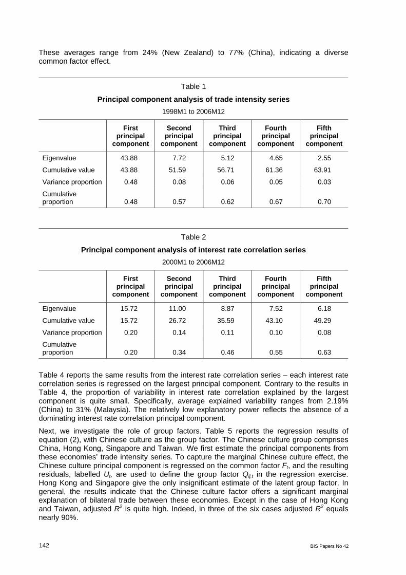
As discussed in the previous section, the principal component approach is used to extract from the trade intensity series the common factors that drive the evolution of bilateral trade among the sample economies. Table 1 shows the five largest principal components, which explain 70% of the total variation. The largest principal component accounts for around 44% of the total variation. The presence of a strong common component suggests that trade among the 14 sample economies is driven by an influential common latent factor.

7 There are other measures of financial integration, such as interest rate parity conditions and financial

openness. See, for example, Cheung, Chinn and Fujii (2007).

0.5 1.0 1.5 2.0 2.5 3.0 3.5

98 99 00 01 02 03 04 05 06

C hi na v s Ja pa n

0

0.2

0.4

0.6

0.8

98 99 00 01 02 03 04 05 06

China vs India

0.6

0.8

1.0

1.2

1.4

1.6

1.8

98 99 00 01 02 03 04 05 06

Japan v s Kore a

4 6 8

10 12 14 16

98 99 00 01 02 03 04 05 06

C hi n a v s H ong K on g

0.4 0.8 1.2 1.6 2.0 2.4

98 99 00 01 02 03 04 05 06

China vs Singapore

3

4

5

6

7

8

9

98 99 00 01 02 03 04 05 06

Hong Kong v s T a i w an

16 18 20 22 24 26 28

98 99 00 01 02 03 04 05 06

S i ngap ore v s M al a y si a

3 4 5 6 7 8

98 99 00 01 02 03 04 05 06

S i ngapore vs Thailand

0.3

0.4

0.5

0.6

0.7

0.8

0.9

98 99 00 01 02 03 04 05 06

Japan vs Aust ral ia


Figure 2

Selected interest rate correlation series 2000M1 to 2006M12

Table 2 describes the five largest principal components derived from the interest rate correlation series. Unlike the trade intensity series, the interest rate correlation series do not display a dominant principal component. The largest principal component accounts for only 16% of the total variation, whereas each of the next three largest principal components accounts for more than 10% of the total variation. The evidence indicates that, compared with the trade intensity series, the interest rate correlation series have relatively weak common components. The result should not be too surprising because the interest rate is an instrument of the monetary policy pursued by these economies to manage diverse economic conditions.8 Further, most of these economies do not have full capital account convertibility.

To investigate the relevance of the largest principal component, we estimate equation (1) and calculate the proportion of trade intensity variation explained by the common factor Ft. The results are presented in Table 3. The common factor plays a significant role in explaining the bilateral trade of China, Japan and India, the three largest economies in the region. The average of the explained variability for each economy is shown in the last row of the table.

8 Hong Kong may be the only exception in the group, given its currency board arrangement, which pegs the

Hong Kong dollar to the US dollar.

–1.0

–0.5

0.0

0.5

1.0

00 01 02 03 04 05 06

C h i na v s Japan

–1.0

–0.5

0.0

0.5

1.0

00 01 02 03 04 05 06

China vs India

–0.8

–0.4

0.0

0.4

0.8

1.2

00 01 02 03 04 05 06

Japan v s K o re a

–1.2 –0.8 –0.4 0.0 0.4 0.8

00 01 02 03 04 05 06

C hi n a v s H ong Kon g

–1.0

–0.5

0.0

0.5

1.0

00 01 02 03 04 05 06

China vs Singapore

–0.8

–0.4

0.0

0.4

0.8

1.2

00 01 02 03 04 05 06

H o n g Kong v s T ai w an

–1.0

–0.5

0.0

0.5

1.0

00 01 02 03 04 05 06

Si ngap ore v s Malay s ia

–0.8 –0.4 0.0 0.4 0.8 1.2

00 01 02 03 04 05 06

Singapore vs Thailand

–1.0

–0.5

0.0

0.5

1.0

00 01 02 03 04 05 06

Japa n v s A us tra l i a


These averages range from 24% (New Zealand) to 77% (China), indicating a diverse common factor effect.

Table 1

Principal component analysis of trade intensity series 1998M1 to 2006M12

First

principal component

Second principal

component

Third principal

component

Fourth principal

component

Fifth principal

component

Eigenvalue 43.88 7.72 5.12 4.65 2.55

Cumulative value 43.88 51.59 56.71 61.36 63.91

Variance proportion 0.48 0.08 0.06 0.05 0.03

Cumulative proportion 0.48 0.57 0.62 0.67 0.70

Table 2

Principal component analysis of interest rate correlation series 2000M1 to 2006M12

First

principal component

Second principal

component

Third principal

component

Fourth principal

component

Fifth principal

component

Eigenvalue 15.72 11.00 8.87 7.52 6.18




Table 4 reports the same results from the interest rate correlation series – each interest rate correlation series is regressed on the largest principal component. Contrary to the results in Table 4, the proportion of variability in interest rate correlation explained by the largest component is quite small. Specifically, average explained variability ranges from 2.19% (China) to 31% (Malaysia). The relatively low explanatory power reflects the absence of a dominating interest rate correlation principal component.

Next, we investigate the role of group factors. Table 5 reports the regression results of equation (2), with Chinese culture as the group factor. The Chinese culture group comprises China, Hong Kong, Singapore and Taiwan. We first estimate the principal components from these economies’ trade intensity series. To capture the marginal Chinese culture effect, the Chinese culture principal component is regressed on the common factor Ft, and the resulting residuals, labelled Ut, are used to define the group factor Qij,t in the regression exercise. Hong Kong and Singapore give the only insignificant estimate of the latent group factor. In general, the results indicate that the Chinese culture factor offers a significant marginal explanation of bilateral trade between these economies. Except in the case of Hong Kong and Taiwan, adjusted R2 is quite high. Indeed, in three of the six cases adjusted R2 equals nearly 90%.


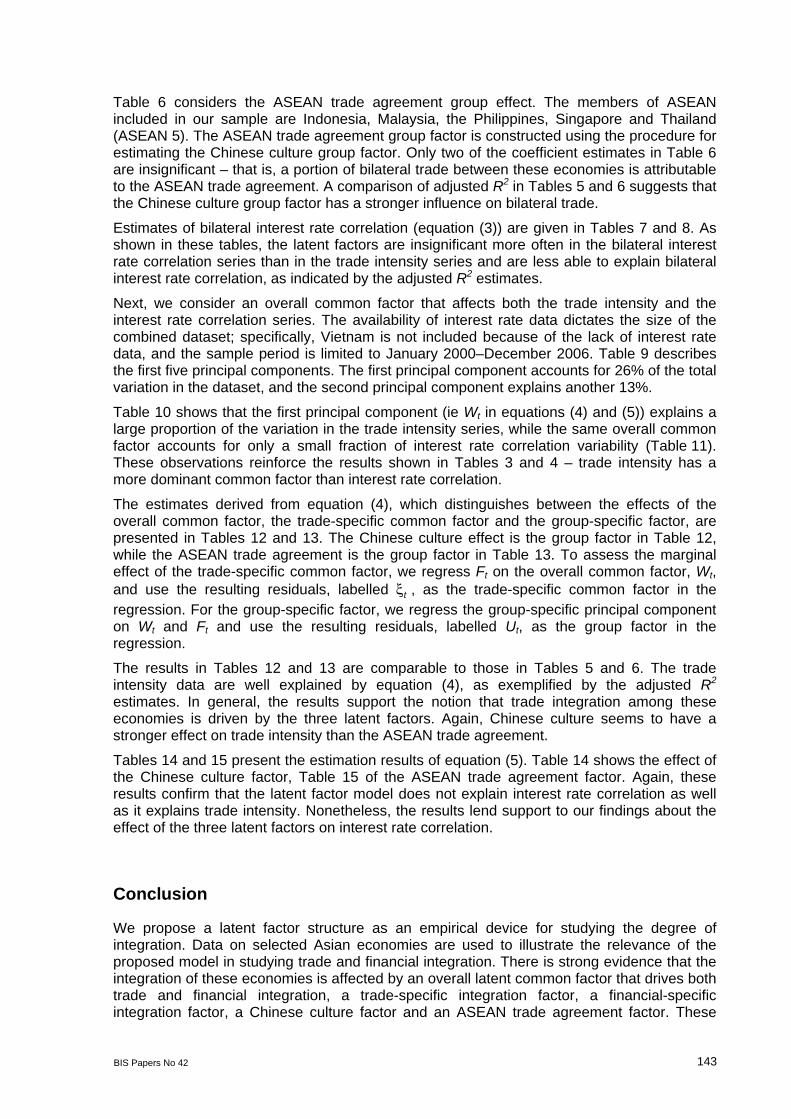
Table 6 considers the ASEAN trade agreement group effect. The members of ASEAN included in our sample are Indonesia, Malaysia, the Philippines, Singapore and Thailand (ASEAN 5). The ASEAN trade agreement group factor is constructed using the procedure for estimating the Chinese culture group factor. Only two of the coefficient estimates in Table 6 are insignificant – that is, a portion of bilateral trade between these economies is attributable to the ASEAN trade agreement. A comparison of adjusted R2 in Tables 5 and 6 suggests that the Chinese culture group factor has a stronger influence on bilateral trade.

Estimates of bilateral interest rate correlation (equation (3)) are given in Tables 7 and 8. As shown in these tables, the latent factors are insignificant more often in the bilateral interest rate correlation series than in the trade intensity series and are less able to explain bilateral interest rate correlation, as indicated by the adjusted R2 estimates.

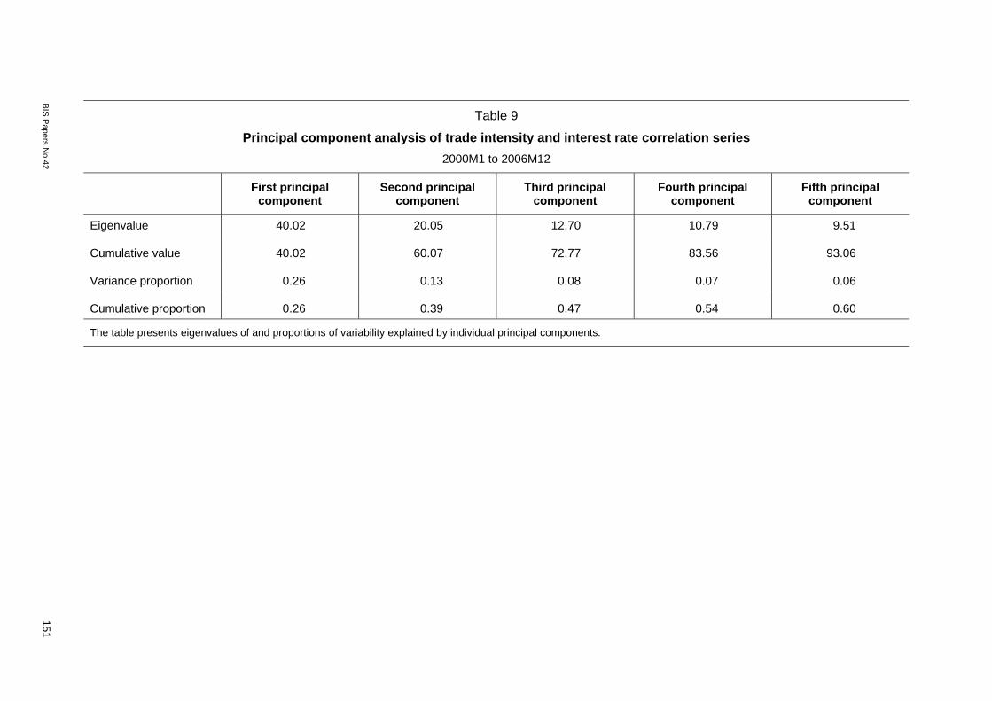
Next, we consider an overall common factor that affects both the trade intensity and the interest rate correlation series. The availability of interest rate data dictates the size of the combined dataset; specifically, Vietnam is not included because of the lack of interest rate data, and the sample period is limited to January 2000–December 2006. Table 9 describes the first five principal components. The first principal component accounts for 26% of the total variation in the dataset, and the second principal component explains another 13%.

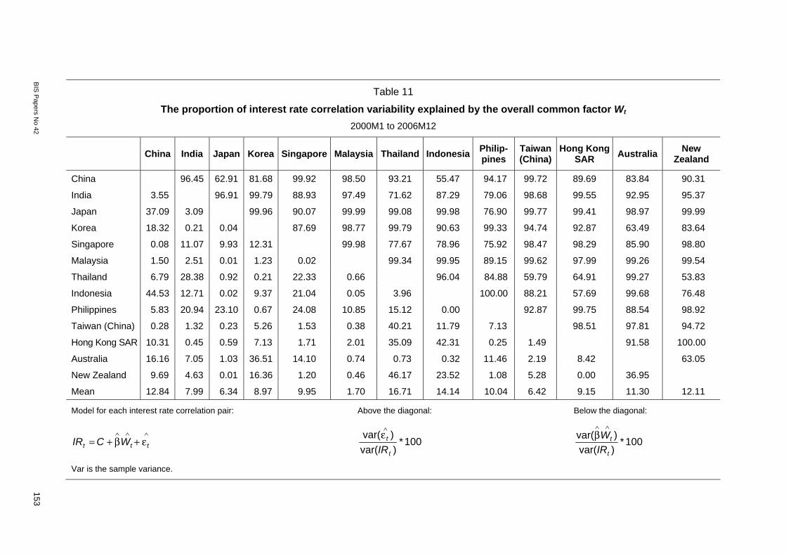
Table 10 shows that the first principal component (ie Wt in equations (4) and (5)) explains a large proportion of the variation in the trade intensity series, while the same overall common factor accounts for only a small fraction of interest rate correlation variability (Table 11). These observations reinforce the results shown in Tables 3 and 4 – trade intensity has a more dominant common factor than interest rate correlation.

The estimates derived from equation (4), which distinguishes between the effects of the overall common factor, the trade-specific common factor and the group-specific factor, are presented in Tables 12 and 13. The Chinese culture effect is the group factor in Table 12, while the ASEAN trade agreement is the group factor in Table 13. To assess the marginal effect of the trade-specific common factor, we regress Ft on the overall common factor, Wt, and use the resulting residuals, labelled tξ , as the trade-specific common factor in the regression. For the group-specific factor, we regress the group-specific principal component on Wt and Ft and use the resulting residuals, labelled Ut, as the group factor in the regression.

The results in Tables 12 and 13 are comparable to those in Tables 5 and 6. The trade intensity data are well explained by equation (4), as exemplified by the adjusted R2 estimates. In general, the results support the notion that trade integration among these economies is driven by the three latent factors. Again, Chinese culture seems to have a stronger effect on trade intensity than the ASEAN trade agreement.

Tables 14 and 15 present the estimation results of equation (5). Table 14 shows the effect of the Chinese culture factor, Table 15 of the ASEAN trade agreement factor. Again, these results confirm that the latent factor model does not explain interest rate correlation as well as it explains trade intensity. Nonetheless, the results lend support to our findings about the effect of the three latent factors on interest rate correlation.

Conclusion

We propose a latent factor structure as an empirical device for studying the degree of integration. Data on selected Asian economies are used to illustrate the relevance of the proposed model in studying trade and financial integration. There is strong evidence that the integration of these economies is affected by an overall latent common factor that drives both trade and financial integration, a trade-specific integration factor, a financial-specific integration factor, a Chinese culture factor and an ASEAN trade agreement factor. These


results are indicative in general of the usefulness of the proposed model in analysing the integration of economies.

We recognise that the current exercise is an exploratory one and that the empirical strategy is not closely linked to any theory of integration. Indeed, in the paper we focus on fitting the data and are sketchy on the related economic interpretation. Currently, we are extending the exercise in several directions. First, we are considering dynamic factor models that allow the latent factors to have time-varying effects on the degree of integration. Obviously, a time-varying latent factor effect offers a means of capturing the possible temporal variation of the link between the latent factor and the degree of integration. Second, the choice of interest rate correlation as a proxy for financial integration may be controversial. We are examining alternative measures of financial integration, including price and interest rate parity conditions. Third, while the proposed factor approach offers a flexible way to study integration, the current framework does not provide much economic interpretation. It is our plan in the next stage to shed some light on the economic intuitions of the exercise by relating the latent common factors to observable economic variables.

BIS P

apers No 42

145

Table 3

The proportion of trade intensity variability explained by the overall common factor Ft 1998M1 to 2006M12

China India Japan Korea Singapore Malaysia Thailand Indonesia Philip-pines

Taiwan(China)

Hong Kong SAR

Viet-nam Australia New

Zealand

China 13.12 6.48 15.30 15.43 24.45 14.62 27.82 24.55 11.62 57.79 31.42 11.47 45.27

India 86.88 56.93 28.66 20.13 69.14 27.95 8.75 92.78 35.57 56.48 8.92 33.63 86.47

Japan 93.52 43.07 26.71 44.18 53.15 7.52 15.93 40.75 26.39 15.01 12.89 24.41 25.85

Korea 84.70 71.34 73.29 99.54 90.98 91.81 100.00 63.61 32.07 72.56 57.64 97.00 94.25

Singapore 84.57 79.87 55.82 0.46 90.87 49.67 24.56 95.70 34.56 9.31 32.80 76.86 47.17

Malaysia 75.55 30.86 46.85 9.02 9.13 11.23 53.91 89.52 72.70 29.92 32.22 89.00 99.70

Thailand 85.38 72.05 92.48 8.19 50.33 88.77 47.48 75.12 44.16 11.26 17.30 31.89 50.70

Indonesia 72.18 91.25 84.07 0.00 75.44 46.09 52.52 99.29 58.52 82.26 89.45 97.49 88.91

Philippines 75.45 7.22 59.25 36.39 4.30 10.48 24.88 0.71 69.02 38.64 86.99 74.09 85.28

Taiwan (China) 88.38 64.43 73.61 67.93 65.44 27.30 55.84 41.48 30.98 84.30 18.91 99.87 68.44

Hong Kong SAR 42.21 43.52 84.99 27.44 90.69 70.08 88.74 17.74 61.36 15.70 20.40 70.38 92.48

Vietnam 68.58 91.08 87.11 42.36 67.20 67.78 82.70 10.55 13.01 81.09 79.60 54.31 99.59

Australia 88.53 66.37 75.59 3.00 23.14 11.00 68.11 2.51 25.91 0.13 29.62 45.69 99.07

New Zealand 54.73 13.53 74.15 5.75 52.83 0.30 49.30 11.09 14.72 31.56 7.52 0.41 0.93

Mean 76.97 58.57 72.60 33.07 50.71 37.94 63.02 38.89 28.05 49.53 50.71 56.71 33.89 24.37

Model for each trading pair: Above the diagonal: Below the diagonal:

∧∧∧ε+γ+= ttt FCTI 100*

)var()var(

t

t

TI

∧ε

100*)var()var(

t

t

TIF∧∧

γ

Var is the sample variance.

146

BIS P

apers No 42

Table 4

The proportion of interest rate correlation variability explained by the common factor Ft 2000M1 to 2006M12


Taiwan (China)

Hong Kong SAR Australia New

Zealand

China 97.02 98.61 95.89 99.74 90.15 99.99 98.14 99.93 99.99 99.49 98.40 96.43

India 2.98 91.40 70.98 83.12 48.49 80.89 32.21 95.34 99.92 99.91 62.35 86.44

Japan 1.39 8.60 50.52 86.61 68.78 78.56 61.82 84.91 63.44 86.91 52.59 57.35

Korea 4.11 29.02 49.48 45.35 77.26 78.80 91.58 97.50 54.26 70.68 89.13 85.23

Singapore 0.26 16.88 13.39 54.65 59.76 96.01 83.45 69.71 75.93 98.01 78.05 80.58

Malaysia 9.85 51.51 31.22 22.74 40.24 54.57 99.20 99.89 36.22 55.36 80.80 57.35

Thailand 0.01 19.11 21.44 21.20 3.99 45.43 52.92 87.03 94.59 94.74 81.56 99.63

Indonesia 1.86 67.79 38.18 8.42 16.55 0.80 47.08 99.24 51.80 63.27 94.64 91.87

Philippines 0.07 4.66 15.09 2.50 30.29 0.11 12.97 0.76 79.07 71.03 84.72 78.72

Taiwan (China) 0.01 0.08 36.56 45.74 24.07 63.78 5.41 48.20 20.93 94.70 64.99 78.83

Hong Kong SAR 0.51 0.09 13.09 29.32 1.99 44.64 5.26 36.73 28.97 5.30 73.19 75.47

Australia 1.60 37.65 47.41 10.87 21.95 19.20 18.44 5.36 15.28 35.01 26.81 84.69

New Zealand 3.57 13.56 42.65 14.77 19.42 42.65 0.37 8.13 21.28 21.17 24.53 15.31

Mean 2.19 21.00 26.54 24.40 20.31 31.01 16.73 23.32 12.74 25.52 18.10 21.24 18.95

Model for each interest rate correlation pair: Above the diagonal: Below the diagonal:

∧∧∧ε+γ+= ttt GCIR 100*

)var()var(

t

t

IR

∧ε

100*)var()var(

t

t

IRG

∧∧γ


BIS P

apers No 42

147

Table 5

Results of regressing trade intensity series on their first principal component and the Chinese culture factor

1998M1 to 2006M12

China

vs Singapore

China vs

Taiwan (China)

China vs

Hong Kong SAR

Singapore vs

Taiwan (China)

Singapore vs

Hong Kong SAR

Taiwan (China) vs

Hong Kong SAR

Constant 1.14 (0.00) 1.37 (0.00) 9.48 (0.00) 2.22 (0.00) 7.15 (0.00) 6.84 (0.00)

First principal component (Ft) 0.06 (0.00) 0.13 (0.00) 0.21 (0.00) 0.06 (0.00) 0.27 (0.00) 0.05 (0.00)

Ut 0.18 (0.00) 0.21 (0.00) 2.26 (0.00) 0.14 (0.01) –0.01 (0.93) 0.56 (0.00)

R2 0.89 0.90 0.71 0.68 0.91 0.27

Adj. R2 0.89 0.90 0.70 0.67 0.91 0.26

Ut is the residual series obtained from regressing the first Chinese culture principal component on the first principal component of the trading intensity series. ( ) contains the p-value of parameter estimate.

148

BIS P

apers No 42

Table 6

Results of regressing trade intensity series on their first principal component and the ASEAN 5 factor

1998M1 to 2006M12

Singapore

vs Malaysia

Singaporevs

Thailand

Singaporevs

Indonesia

Singaporevs

Philippines

Malaysia vs

Thailand

Malaysia vs

Indonesia

Malaysia vs

Philippines

Thailand vs

Indonesia

Thailand vs

Philippines

Indonesia vs

Philippines

Constant 20.73 (0.00) 5.31 (0.00) 5.16 (0.00) 3.35 (0.00) 3.30 (0.00) 1.42 (0.00) 1.82 (0.00) 0.98 (0.00) 1.13 (0.00) 0.41 (0.00)

First principal component (Ft) 0.09 (0.00) 0.06 (0.00) 0.25 (0.00) 0.01 (0.01) 0.11 (0.00) 0.02 (0.00) 0.01 (0.00) 0.03 (0.00) 0.02 (0.00) –0.001 (0.34)

Ut 1.45 (0.00) 0.29 (0.00) 0.02 (0.82) 0.23 (0.00) 0.12 (0.00) 0.09 (0.00) 0.08 (0.00) 0.06 (0.00) 0.08 (0.00) 0.04 (0.00)

R2 0.58 0.73 0.75 0.27 0.91 0.61 0.18 0.57 0.37 0.17

Adj. R2 0.57 0.73 0.75 0.26 0.91 0.60 0.16 0.56 0.36 0.16

Ut is the residual series obtained from regressing the first ASEAN trade agreement principal component on the first principal component of the trading intensity series. ( ) contains the p-value of parameter estimate.

BIS P

apers No 42

149

Table 7

Results of regressing interest rate correlation series on their first principal component and the Chinese culture factor

2000M1 to 2006M12

China

vs Singapore

China vs

Taiwan (China)

China vs

Hong Kong SAR

Singapore vs

Taiwan (China)

Singapore vs

Hong Kong SAR

Taiwan (China) vs

Hong Kong SAR

Constant 0.04 (0.16) –0.02 (0.65) –0.14 (0.00) 0.54 (0.00) 0.56 (0.00) 0.62 (0.00)

First principal component (Gt) –0.01 (0.40) –0.001 (0.87) –0.01 (0.46) 0.05 (0.00) 0.01 (0.11) 0.02 (0.01)

Ut 0.23 (0.00) 0.26 (0.00) 0.16 (0.00) –0.13 (0.00) –0.12 (0.00) –0.14 (0.00)

R2 0.70 0.59 0.27 0.52 0.39 0.44

Adj. R2 0.70 0.58 0.25 0.51 0.37 0.43

Ut is the residual series obtained from regressing the first Chinese culture principal component on the first principal component of the interest rate correlation series. ( ) contains the p-value of parameter estimate.

150

BIS P

apers No 42

Table 8

Results of regressing interest rate correlation series on their first principal component and the ASEAN 5 factor

2000M1 to 2006M12

Singapore

vs Malaysia

Singaporevs

Thailand

Singaporevs

Indonesia

Singaporevs

Philippines

Malaysia vs

Thailand

Malaysia vs

Indonesia

Malaysia vs

Philippines

Thailand vs

Indonesia

Thailand vs

Philippines

Indonesia vs

Philippines

Constant 0.12 (0.00) 0.40 (0.00) –0.004 (0.92) –0.08 (0.02) 0.11 (0.00) 0.04 (0.46) 0.39 (0.00) 0.32 (0.00) 0.19 (0.00) 0.14 (0.00)

First principal component (Gt) 0.09 (0.00) 0.02 (0.07) –0.04 (0.00) 0.07 (0.00) 0.10 (0.00) –0.01 (0.28) –0.003 (0.77) –0.08 (0.00) 0.05 (0.00) –0.01 (0.14)

Ut 0.17 (0.00) –0.01 (0.67) 0.06 (0.03) 0.18 (0.00) 0.23 (0.00) 0.26 (0.00) 0.04 (0.15) 0.06 (0.01) 0.25 (0.00) 0.23 (0.00)

R2 0.63 0.04 0.21 0.64 0.82 0.46 0.03 0.51 0.75 0.73

Adj. R2 0.62 0.02 0.19 0.63 0.82 0.44 0.002 0.50 0.75 0.72

Ut is the residual series obtained from regressing the first ASEAN trade agreement principal component on the principal component of the interest rate correlation series. ( ) contains the p-value of parameter estimate.

BIS P

apers No 42

151

Table 9

Principal component analysis of trade intensity and interest rate correlation series 2000M1 to 2006M12

First principal component

Second principal component

Third principal component

Fourth principal component

Fifth principal component

Eigenvalue 40.02 20.05 12.70 10.79 9.51




The table presents eigenvalues of and proportions of variability explained by individual principal components.

152

BIS P

apers No 42

Table 10

The proportion of trade intensity variability explained by the overall common factor Wt 1998M1 to 2006M12


Taiwan (China)


Zealand

China 15.92 7.73 19.87 18.22 35.85 20.45 41.37 22.05 9.31 60.13 17.47 57.56

India 84.08 47.99 14.03 21.48 41.93 43.64 9.09 99.99 42.55 64.94 25.64 72.20

Japan 92.27 52.01 28.44 60.44 87.82 10.35 31.40 62.31 38.43 18.31 26.09 20.04

Korea 80.13 85.97 71.56 92.73 99.72 97.87 95.74 69.91 48.49 73.18 94.26 98.20

Singapore 81.78 78.52 39.56 7.27 99.97 74.61 12.25 99.50 57.75 11.20 91.40 42.84

Malaysia 64.15 58.07 12.18 0.28 0.03 17.08 57.60 86.97 93.63 39.97 97.86 98.37

Thailand 79.55 56.36 89.65 2.13 25.39 82.92 41.34 99.98 58.27 19.14 53.63 71.65

Indonesia 58.63 90.91 68.60 4.26 87.75 42.40 58.66 99.79 71.58 90.55 87.69 98.67

Philippines 77.95 0.01 37.69 30.09 0.50 13.03 0.02 0.21 97.52 47.77 60.08 99.57

Taiwan (China) 90.69 57.45 61.57 51.51 42.25 6.37 41.73 28.42 2.48 99.52 99.97 69.83

Hong Kong SAR 39.87 35.06 81.69 26.82 88.80 60.03 80.86 9.45 52.23 0.48 62.13 95.69

Australia 82.53 74.36 73.91 5.74 8.60 2.14 46.37 12.31 39.92 0.03 37.87 95.94

New Zealand 42.44 27.80 79.96 1.80 57.16 1.63 28.35 1.33 0.43 30.17 4.31 4.06

Mean 72.84 58.38 63.39 30.63 43.13 28.60 49.33 38.58 21.21 34.43 43.12 32.32 23.29

Model for each trading pair: Above the diagonal: Below the diagonal:

∧∧∧+β+= ttt vWCTI 100*

)var()var(

t

t

TIv

∧

100*)var()var(

t

t

TIW

∧∧β


BIS P

apers No 42

153

Table 11

The proportion of interest rate correlation variability explained by the overall common factor Wt 2000M1 to 2006M12


Taiwan (China)


Zealand

China 96.45 62.91 81.68 99.92 98.50 93.21 55.47 94.17 99.72 89.69 83.84 90.31

India 3.55 96.91 99.79 88.93 97.49 71.62 87.29 79.06 98.68 99.55 92.95 95.37

Japan 37.09 3.09 99.96 90.07 99.99 99.08 99.98 76.90 99.77 99.41 98.97 99.99

Korea 18.32 0.21 0.04 87.69 98.77 99.79 90.63 99.33 94.74 92.87 63.49 83.64

Singapore 0.08 11.07 9.93 12.31 99.98 77.67 78.96 75.92 98.47 98.29 85.90 98.80

Malaysia 1.50 2.51 0.01 1.23 0.02 99.34 99.95 89.15 99.62 97.99 99.26 99.54

Thailand 6.79 28.38 0.92 0.21 22.33 0.66 96.04 84.88 59.79 64.91 99.27 53.83

Indonesia 44.53 12.71 0.02 9.37 21.04 0.05 3.96 100.00 88.21 57.69 99.68 76.48

Philippines 5.83 20.94 23.10 0.67 24.08 10.85 15.12 0.00 92.87 99.75 88.54 98.92

Taiwan (China) 0.28 1.32 0.23 5.26 1.53 0.38 40.21 11.79 7.13 98.51 97.81 94.72

Hong Kong SAR 10.31 0.45 0.59 7.13 1.71 2.01 35.09 42.31 0.25 1.49 91.58 100.00

Australia 16.16 7.05 1.03 36.51 14.10 0.74 0.73 0.32 11.46 2.19 8.42 63.05

New Zealand 9.69 4.63 0.01 16.36 1.20 0.46 46.17 23.52 1.08 5.28 0.00 36.95

Mean 12.84 7.99 6.34 8.97 9.95 1.70 16.71 14.14 10.04 6.42 9.15 11.30 12.11

Model for each interest rate correlation pair: Above the diagonal: Below the diagonal:

∧∧∧ε+β+= ttt WCIR 100*

)var()var(

t

t

IR

∧ε

100*)var()var(

t

t

IRW

∧∧β


154

BIS P

apers No 42

Table 12

Results of regressing trade intensity series on Wt, their first principal component and the Chinese culture factor

2000M1 to 2006M12

China

vs Singapore

China vs

Taiwan (China)

China vs

Hong Kong SAR

Singapore vs

Taiwan (China)

Singapore vs

Hong Kong SAR

Taiwan (China) vs

Hong Kong SAR

Constant 1.24 (0.00) 1.64 (0.00) 9.81 (0.00) 2.37 (0.00) 7.68 (0.00) 7.03 (0.00)

Overall common factor (Wt) 0.06 (0.00) 0.12 (0.00) 0.21 (0.00) 0.04 (0.00) 0.27 (0.00) 0.01 (0.48)

tξ 0.08 (0.00) –0.07 (0.00) 0.58 (0.00) 0.15 (0.00) 0.21 (0.00) 0.34 (0.00)

Ut 0.21 (0.00) 0.35 (0.00) 2.21 (0.00) 0.12 (0.07) –0.17 (0.22) 0.37 (0.02)

R2 0.91 0.95 0.74 0.56 0.90 0.26

Adj. R2 0.91 0.95 0.73 0.55 0.90 0.23

tξ is the residual series obtained from regression Ft on Wt. Ut is the residual series obtained from regressing the first Chinese culture principal component on Wt and Ft. ( ) contains the p-value of the parameter estimate.

BIS P

apers No 42

155

Table 13

Results of regressing trade intensity series on Wt, their first principal component and the ASEAN 5 factor

2000M1 to 2006M12

Singapore

vs Malaysia

Singaporevs

Thailand

Singaporevs

Indonesia

Singaporevs

Philippines

Malaysia vs

Thailand

Malaysia vs

Indonesia

Malaysia vs

Philippines

Thailand vs

Indonesia

Thailand vs

Philippines

Indonesia vs

Philippines

Constant 21.06 (0.00) 5.47 (0.00) 5.53 (0.00) 3.42 (0.00) 3.58 (0.00) 1.46 (0.00) 1.84 (0.00) 1.04 (0.00) 1.22 (0.00) 0.40 (0.00)

Overall common factor (Wt) –0.00 (0.78) 0.04 (0.00) 0.29 (0.00) –0.01 (0.48) 0.09 (0.00) 0.02 (0.00) 0.02 (0.00) 0.03 (0.00) 0.00 (0.89) 0.00 (0.62)

tξ 1.23 (0.00) 0.24 (0.00) –0.14 (0.06) 0.18 (0.00) 0.02 (0.40) 0.08 (0.00) –0.02 (0.59) –0.02 (0.26) 0.04 (0.01) –0.00 (0.90)

Ut 1.02 (0.00) 0.23 (0.00) 0.25 (0.00) 0.12 (0.02) 0.17 (0.00) 0.09 (0.00) 0.08 (0.00) 0.09 (0.00) 0.03 (0.05) 0.05 (0.00)

R2 0.72 0.69 0.90 0.20 0.91 0.72 0.22 0.72 0.11 0.33

Adj. R2 0.71 0.68 0.89 0.17 0.90 0.71 0.19 0.71 0.08 0.30

tξ is the residual series obtained from regression Ft on Wt . Ut is the residual series obtained from regressing the first ASEAN trade agreement principal component on Wt and Ft. ( ) contains the p-value of the parameter estimate.

156

BIS P

apers No 42

Table 14

Results of regressing interest rate correlation series on Wt, their first principal component and the Chinese culture factor

2000M1 to 2006M12

China

vs Singapore

China vs

Taiwan (China)

China vs

Hong Kong SAR

Singapore vs

Taiwan (China)

Singapore vs

Hong Kong SAR

Taiwan (China) vs

Hong Kong SAR

Constant 0.04 (0.16) –0.02 (0.66) –0.14 (0.00) 0.54 (0.00) 0.56 (0.00) 0.62 (0.00)

Overall common factor (Wt) –0.00 (0.65) –0.00 (0.46) –0.02 (0.00) 0.01 (0.10) –0.01 (0.13) –0.01 (0.14)

Ut –0.01 (0.32) –0.00 (0.71) –0.02 (0.08) 0.06 (0.00) 0.01 (0.20) 0.02 (0.01)

tξ 0.23 (0.00) 0.27 (0.00) 0.15 (0.00) –0.13 (0.00) –0.13 (0.00) –0.14 (0.00)

R2 0.71 0.59 0.35 0.56 0.41 0.46

Adj. R2 0.70 0.58 0.33 0.54 0.39 0.44

tξ is the residual series obtained from regression Gt on Wt. Ut is the residual series obtained from regressing the first Chinese culture principal component on Wt and Gt. ( ) contains the p-value of the parameter estimate.

BIS P

apers No 42

157

Table 15

Results of regressing interest rate correlation series on Wt, their first principal component and the ASEAN 5 factor

2000M1 to 2006M12

Singapore

vs Malaysia

Singaporevs

Thailand

Singaporevs

Indonesia

Singaporevs

Philippines

Malaysia vs

Thailand

Malaysia vs

Indonesia

Malaysia vs

Philippines

Thailand vs

Indonesia

Thailand vs

Philippines

Indonesia vs

Philippines

Constant 0.12 (0.00) 0.40 (0.00) –0.00 (0.92) –0.08 (0.01) 0.11 (0.00) 0.04 (0.46) 0.39 (0.00) 0.32 (0.00) 0.19 (0.00) 0.14 (0.00)

Overall common factor (Wt) 0.00 (0.82) 0.04 (0.00) 0.03 (0.00) –0.04 (0.00) 0.01 (0.01) 0.00 (0.79) –0.02 (0.00) 0.01 (0.01) –0.03 (0.00) 0.00 (0.94)

Ut 0.09 (0.00) 0.04 (0.00) –0.03 (0.00) 0.06 (0.00) 0.11 (0.00) –0.01 (0.30) –0.01 (0.25) –0.08 (0.00) 0.04 (0.00) –0.01 (0.13)

tξ 0.17 (0.00) –0.00 (0.95) 0.07 (0.01) 0.17 (0.00) 0.24 (0.00) 0.26 (0.00) 0.03 (0.20) 0.06 (0.01) 0.25 (0.00) 0.23 (0.00)

R2 0.68 0.33 0.34 0.74 0.92 0.46 0.14 0.51 0.81 0.73

Adj. R2 0.66 0.31 0.34 0.73 0.91 0.44 0.11 0.49 0.81 0.72

tξ is the residual series obtained from regression Gt on Wt . Ut is the residual series obtained from regressing the first ASEAN trade agreement principal component on Wt and Gt. ( ) contains the p-value of the parameter estimate.


References

Bayoumi, T (1997): Financial integration and real activity, University of Michigan Press.

Chamberlain, G and M Rothschild (1983): “Arbitrage factor structure, and mean-variance analysis on large asset markets”, Econometrica, vol 51, no 5, September, pp 1281–304.

Cheung, Y, M Chinn and E Fujii (2007): The economic integration of greater China: real and financial linkages and the prospects for currency union, Hong Kong University Press.

Eatwell, J, M Milgate and P Newman (1987): The new Palgrave: a dictionary of economics, Palgrave Macmillan.

Forni, M and L Reichlin (1998): “Let’s get real: a dynamic factor analytical approach to dis-aggregated business cycle”, The Review of Economic Studies, vol 65, no 3, July, pp 453–73.

Forni, M, M Hallin, M Lippi and L Reichlin (2000): “The generalized dynamic-factor model: identification and estimation”, The Review of Economics and Statistics, vol 82, no 4, November, pp 540–54.

Giannone, D, L Reichlin and D Small (2005): “Nowcasting GDP and inflation: the real time informational content of macroeconomic data releases”, Board of Governors of the US Federal Reserve System Finance and Economic Discussion Series, no 2005–42.

International Monetary Fund (2002): World economic outlook: trade and finance, Washington, September.

McCauley, R, S S Fung and B Gadanecz (2002): “Integrating the finances of East Asia”, BIS Quarterly Review, December, pp 83–96.

Mody, A and A Murshid (2002): “Growing up with capital flows”, IMF Working Papers, no 02/75, Washington, April.

Obstfeld, M and A Taylor (2004): Global capital markets: integration, crisis, and growth, Cambridge University Press.

Stock, J H and M W Watson (1989): “New indexes of coincident and leading economic indicators”, in O J Blanchard and S Fischer (eds), NBER Macroeconomics Annual 1989, pp 351–94.

——— (2002a): “Forecasting using principal components from a large number of predictors”, Journal of the American Statistical Association, vol 97, December, pp 1167–79.

——— (2002b): “Macroeconomic forecasting using diffusion indexes”, Journal of Business & Economic Statistics, vol 20, no 2, April, pp 147–62.

Yu, I, L Fung and C Tam (2007): “Assessing bond market integration in Asia”, Hong Kong Monetary Authority Working Papers, no 0710.

Measuring economic integration: the case of Asian economies - BIS

Documents

Transcript of Measuring economic integration: the case of Asian economies - BIS