McAlevey House Prices Disposable Income Permanent ...

1

House Prices, Disposable Income, and Permanent and Temporary Shocks

Patricia Fraser*, Martin Hoesli**

and Lynn McAlevey***

Abstract

This paper specifies a two-variable system of house prices and income for New

Zealand, the U.K. and the U.S., covering periods from 1973:4 through 2008:2. The

analysis allows the identification of differences in house price−income relationships over sub-periods and, using a SVAR approach, compares the responses of house

prices when faced with permanent and transitory shocks to income. It continues by

decomposing each historical house price series into their permanent, temporary and

deterministic components. Our results suggest that while real house prices have a

long-run relationship with real income in all three economies, the responsiveness of

house prices to innovations in income will vary over both time and markets depending

on whether the income disturbances are viewed as permanent or temporary. The

evidence suggests that New Zealand and U.K. housing markets are sensitive to both

permanent and transitory shocks to income, while the U.S. market reacts to temporary

shocks with the permanent component having a largely insignificant role to play in

house price composition. In New Zealand, the temporary component of house prices

has tended to be positive over time, pushing prices higher than they would have been

otherwise; while in the U.K. both permanent and temporary components have tended

to reinforce each other. Overall, there is no clear consistent global pattern regarding

the importance of these shocks which implies that housing markets will react

differently to the vagaries of global and domestic economic activity driving such

shocks.

JEL Codes: R31, E64

Keywords: House prices, permanent income shocks, temporary income shocks,

SVAR approach

* School of Economics and Finance, Curtin Business School, Curtin University of Technology, GPO

Box U1987, Perth WA 6845 and University of Aberdeen Business School, University of Aberdeen,

Edward Wright Building, Dunbar Street, Aberdeen AB24 3QK, , email: [email protected]

** University of Geneva (HEC and SFI), 40 boulevard du Pont-d’Arve, CH-1211 Geneva 4,

Switzerland, University of Aberdeen Business School, University of Aberdeen, Edward Wright

Building, Dunbar Street, Aberdeen AB24 3QK, Scotland, and Bordeaux Ecole de Management, 680

cours de la Libération, F-33405 Talence cedex, France, email: [email protected] (contact author)

*** Department of Finance and Quantitative Analysis, University of Otago, PO Box 56, Dunedin, New

Zealand, email: [email protected]

We thank Donald Haurin and Elias Oikarinen for very helpful comments on an earlier draft.

2

1. Introduction

It is a stylized fact, supported by empirical research, that a major determinant of house

prices is income. Indeed many researchers have utilized this axiom as a basis from

which to build theoretical and empirical models. Traditionally, income is included as

a key determining factor in equilibrium pricing models, along with variables such as

employment, constructions costs, and interest rates (Bourassa, Hendershott and

Murphy, 2001, Capozza, Hendershott and Mack, 2004). Variations on the present

value model have also been the focus of attention in deriving fundamental values of

house prices (see e.g. Clayton, 1996, Chan, Lee and Woo, 2001, Fraser, Hoesli and

McAlevey, 2008a). The latter studies are motivated by the fact that current and future

‘affordability’ of residential housing has become a strategic issue to informing policy

at both microeconomic and macroeconomic levels of activity. More recent studies

utilizing income discount modeling have incorporated forward-looking and dynamic

characteristics in order to incorporate information regarding expectations on future

income, with this being discounted at a, possibly time-varying, rate of return

representing current and future states of the economy (see e.g. Fraser; Hoesli and

McAlevey, 2008a).

However, one of the key assumptions underlying aforementioned formulations

is that the price−income relationship is constant over time. This, however, is unlikely

to be the case, as reported for instance by Malpezzi (1999) for various U.S. cities.

This view is also supported by wide variations in estimates of reported income

elasticities as measured by the average response of housing expenditure to income.

Tse and Raftery (1999), for example, report elasticity estimates for Hong Kong which

range from 0.1 to 1.4 depending on geographical area, socioeconomic factors, future

income expectations as well as the time period under investigation.

One reason for the time-varying nature of the relationship may itself arise

from the endogenous nature of house prices and income in that both variables are

exposed to two (common) types of macroeconomic shocks: permanent or long-lasting

shocks, e.g. supply-type disturbances such as those involving productivity or enduring

statutory/regulatory changes, and temporary shocks e.g. demand-type disturbances

such as cyclical fiscal or monetary changes. Generally, permanent shocks are those

types of events which provide an impetus for rising/falling (non-stationary) long-term

trends in house prices and income, while transitory shocks are those which drive

3

(stationary) deviations from these long-term trends and therefore account for the

mean-reverting behavior of real house price returns and real income growth.1

While shocks which impinge on income are likely to have much in common

with those affecting house prices, the responsiveness of house prices to income

disturbances may differ according to whether such shocks are viewed as being of a

permanent or transitory nature. While the importance of permanent and temporary

components of income has been consistently recognized in the housing literature (see,

e.g., Lee, 1968, Horioka, 1988, Tse and Rafferty, 1999), the tendency has been to

proxy these components indirectly by using, for example, household level data or

consumption data, rather than recovering the permanent and temporary components

directly from the jointly determined system of prices and income itself: it is this direct

method of estimation which is a key aim of this study.

Consistent with recent studies, this paper proceeds by using time series

methodologies on three major house-owning economies, namely the U.S., the U.K.

and New Zealand (N.Z.). The homeownership rate in these countries is comparable

and high (68% for the U.K. and New Zealand and 66% for the U.S.).2 These

countries, however, vary in that the building regulations, zoning, and population

density, among other things, are quite different. The U.K. has very strict regulations

and is also the most heavily populated. Regulations are more lax in the U.S. and the

country is also far less densely populated. This converts into significantly higher

price elasticities of housing supply in the U.S. than in the U.K. (e.g., Catte et al.,

2004). New Zealand is the least densely populated of the three countries, but building

regulations are stricter than in the U.S. Moreover, construction labor shortages in

periods of rapid growth due in part to emigration have led to construction being to

some extent curtailed. There is empirical evidence to suggest that the supply

elasticity, for Auckland in any case, is closer to that of the U.K. than that of the U.S.

(Grimes et al., 2007).

The three countries differ also with respect to temporary influences on income.

Using deviations from long-term trends, Fraser, Hoesli and McAlevey (2008b)

1 The traditional view in the consumption-income literature is that permanent (temporary) shocks to

income have a marginal propensity to consume (MPC) from permanent income close to unity while the

MPC from transitory income is close to zero. Permanent (temporary) shocks are typically explained as

shocks to non-capital (capital) income (see e.g. Carroll, 2001). However, it is not clear what this

implies for house prices as householders have both consumption and investment motives for holding

residential property and this may vary over time and region. 2 Bourassa and Hoesli (2010).

4

indicate that for the U.K., temporary components of income were predominately

negative between 1984 through 2003, while for N.Z., with the exception of the mid-

late 1990s, income deviations from long-term trend were predominately positive. A

similar exercise for the U.S. indicates that from 1984 through 1991, temporary

components of income were positive, negative until 1998 and positive again until

2004.

Data from these three economies are first analyzed to examine whether a long-

run stable relationship exists between real house prices and real disposable income

and, if so, how prices (on average, over the short-run and long-run) respond to

changes in income and how quickly these prices adjust to the long-run sustainable

relationship. Unlike previous studies, the two elasticity measures along with the

adjustment parameter are estimated simultaneously within an error correction

equation. By abstracting from short-run deviations from possible jointly determined

long-run relationships, not only does this initial analysis allow us to specify the nature

of each of the two-variable systems, it also allows the identification of possible

differences in the house price−income relationships over sub-periods.

While the above analysis is useful in determining the time series

characteristics of the house price–income relationship, it is not however able to

distinguish between the impact on house prices of permanent and transitory income

shocks to each of the two-variable systems. Hence this study further adds to the

existing literature by employing a version of the Blanchard and Quah (1989) (BQ)

methodology which puts restrictions on the Bivariate Moving Average (BMAR)

process to recover the permanent and temporary income disturbances driving the

house price series. Such a method is useful as it allows us to model the relevant

variable innovations within the economic model itself and is applicable to any series

where time series behavior is jointly determined. We can therefore analyze the

impact of permanent and temporary shocks to income on house prices and using a

structural decomposition, analyze the time path of the permanent and temporary

components of house prices in order to gauge the joint impact and importance of these

two types of shocks on house prices over time.

Essentially, the two main objectives of the study, namely, to analyze the

dynamic characteristics of the house price−income relationship over time and to

assess the importance of common temporary and permanent shocks on historical

5

house prices, has value-added in that it provides a comprehensive knowledge base on

which market analysts and policy-makers can form forecasts and derive relevant

policy decisions on the likely path of house prices. Not least, in light of (often

recurring) crises in housing markets and the vagaries of domestic and world-wide

economic activity it is important to gauge how prices in these three developed and

major home-owning economies will behave when faced with different types of

income shocks (see e.g. Goodhart and Hofmann, 2007; Oikarinen, 2009a).

The remainder of this paper is organized as follows. We first present our

empirical framework, followed by a discussion of the data and some preliminary

statistics. The empirical results are discussed next, while concluding remarks are

contained in a final section.

2. Empirical Method and Model

As indicated above, our first task is to consider whether a long-run stable relationship

exists between house prices and income, and if so, how house prices (on average)

respond to changes in income and how quickly these prices adjust to the long-run

sustainable relationship. To do this, we use cointegration tests and, if the null of no

cointegration is rejected, model an error correction relationship which, when specified

in a way which corrects for possible small sample bias, will provide simultaneously:

Unbiased estimates of the average short-run and long-run responsiveness of house

prices to changes in income, as well as the adjustment parameter to long-run

equilibrium.

2.1. Cointegration

The usefulness of this methodology in the current analysis essentially comes down to

determining the rank of the long-run impact matrix between real house prices and real

disposable income. If this has rank, r, then there are r cointegrating relationships

between the variables in the system (Xt), or, n-r common stochastic trends, where n is

the number of variables in the system. The stochastic trends are the linear

combinations of Xt, having the ‘common’ feature of not containing the levels of the

error correction term in them (Gonzalo and Granger, 1995). In other words, they are

the long-run forces that create the non-stationary property of the data.

The number of cointegrating vectors reveals the extent of integration of the

variables in the system. In general terms, if n - r = 0 or r = n (full rank), we have the

6

absence of any stochastic trends with all elements in Xt being stationary, (I(0)), and

cointegration is not defined (Gonzalo and Granger, 1995).

If n – r = n or r = 0, there

are no stationary long-run relationships among the elements of Xt. If n – r = 1 or r =

n - 1, there is a single common stochastic trend, hence a single long-run relationship

that creates the non-stationarity of the data.

2.2. Error Correction Model

Evidence of cointegration between the two variables of interest implies we can use an

error correction model (ECM) to estimate elasticities and associated adjustment

parameters to long-run equilibrium. However, unlike most existing studies who use

either the standard Engle and Granger (1987) method (Hort, 1998; Harter-Dreiman,

2004) or the Johansen (1988) approach (Holly and Jones, 1997; Meese and Wallace,

2003) to measure the equilibrium error, here we follow Banerjee et al. (1986), who

point out that standard cointegrating regressions are likely to be subject to substantial

small sample bias with the problem arising because the estimate of the constant in the

equilibrium relationship may vary with the long-run growth rate of the independent

variable (see also Gallin, 2006). Essentially, unless the long run growth rate of the

independent variable is zero, in our case real disposable income, or long-run

elasticities are equal to short-run elasticities, our prior knowledge of the long-run

parameters are not unbiased, thus we do not have the necessary information to

construct the traditional second-stage specification of an ECM, i.e. the disequilibrium

error (see e.g. Thomas, 1996, pp. 385-386).

Banerjee therefore suggests carrying out the estimation of the long-run and

short-run parameters in a single step. Assuming a first order disequilibrium

relationship is observed:

ttttt hpybybbhp εµ ++++= −− 111210 (1)

with the estimating error correction equation:

ttttot yhpybhp ελβλλβ ++−∆+=∆ −− 1111 (2)

where tt yandhp ∆∆ denote changes in (ln) real house prices and (ln) real disposable

income; 11 −− tt yandhp are one period lagged (ln) levels of these variables. λ is the

adjustment parameter estimating the speed of adjustment to long-run equilibrium, b1

is the estimated short-run elasticity and 1β is the estimate of the long-run elasticity of

7

house prices to income, tε is the regression error. If higher order lags are deemed

necessary, then equation (2) is adjusted accordingly.

2.3. Structural VAR (SVAR)

As discussed above, while the ECM is useful in gaining insight into the average

propensities of house prices to respond to changes in income, it is unable to

distinguish between the impact on house prices of permanent and transitory shocks to

income emanating from the wider economy. It is known that in a univariate model

there is no unique way to decompose a variable into its permanent and temporary

components (Enders, 1995). We employ the Blanchard and Quah (1989) (BQ)

method and follow Lee (1995), Hess and Lee (1999) and, more recently, Fraser,

Hoesli and McAlevey (2008a) in placing restrictions on the Bivariate Moving

Average Representation process to recover the permanent and temporary shocks (see

also Bloch, Fraser and MacDonald, 2009). Such decomposition is useful as it allows

us to model the series disturbances using economic analysis and can be applied to any

series whose time series behaviour is jointly determined. The model is briefly

described below.

Fraser, Hoesli and McAlevey (2008a) develop a dynamic present value model

of house prices, first applied to stock prices and dividends by Campbell and Shiller

(1989), to the relationship between aggregate house prices and national real

disposable income. Starting from the assumptions that equilibrium rent is the rent

renters are willing to pay and this is constrained by income and, real net rental income

is proportional to real disposable income, the authors express the equilibrium real

value of the aggregate housing stock as a constant proportion of the expected future

value of real disposable income. In particular they show that the house price-income

ratio can be expressed as:

*

0 0

( ) j j

t t t j t t j

j j

hp y E y E r cµ µ∞ ∞

+ += =

− = ∆ − +∑ ∑ (3)

where c* is a constant, t)yhp( − is the (ln) house price-real disposable income ratio,

jty +∆ is real income growth, jtr + is the real discount rate, jµ is a linearization

constant and tE is the expectations operator. Following Lee (1995) if we then assume

that the expected discount rate is linearly related to the rate of expected income

growth, we have:

8

( ) , 0t t j t t jE r E y kα α+ += ∆ + >

(4)

where α and k are constants. Substituting (4) into (3) gives:

0

( ) (1 )j

t t t j

j

hp y E y cµ α∞

+=

− = − ∆ +∑ where *

1

kc c

µ

= − + − (5)

and if we model income as the sum of permanent and temporary components which

respond to shocks, we can then impose restrictions on the jointly determined process.

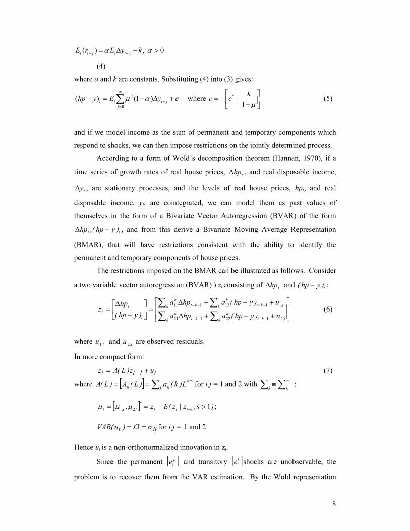
According to a form of Wold’s decomposition theorem (Hannan, 1970), if a

time series of growth rates of real house prices, thp∆ , and real disposable income,

ty∆ , are stationary processes, and the levels of real house prices, hpt, and real

disposable income, yt, are cointegrated, we can model them as past values of

themselves in the form of a Bivariate Vector Autoregression (BVAR) of the form

tt )yhp(,hp −∆ , and from this derive a Bivariate Moving Average Representation

(BMAR), that will have restrictions consistent with the ability to identify the

permanent and temporary components of house prices.

The restrictions imposed on the BMAR can be illustrated as follows. Consider

a two variable vector autoregression (BVAR) ) zt consisting of thp∆ and t)yhp( − :

+−+∆

+−+∆=

−

∆=

−−−−

−−−−

∑∑∑∑

t,ktk

k

ktk

k

t,ktk

k

ktk

k

t

t

tu)yhp(ahpa

u)yhp(ahpa

)yhp(

hpz

2122121

1112111

(6)

where t,u1 and t,u 2 are observed residuals.

In more compact form:

t1tt uz)L(Az += − (7)

where [ ] 1−

∑==k

k ijij L)k(a)L(A)L(A for i,j = 1 and 2 with ∑ ∑∞

≡k k

;

[ ] )s,z|z(Ez, sttt

'

tt,t 121 >−== −µµµ ;

ijt )u(VAR σΩ == for i,j = 1 and 2.

Hence ut is a non-orthonormalized innovation in zt.

Since the permanent [ ]p

te and transitory [ ]t

te shocks are unobservable, the

problem is to recover them from the VAR estimation. By the Wold representation

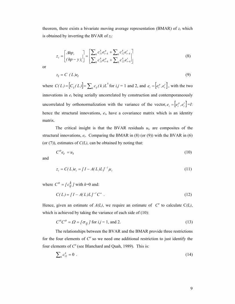
9

theorem, there exists a bivariate moving average representation (BMAR) of zt which

is obtained by inverting the BVAR of zt:

+

+=

−=

−−

−−

∑∑∑∑

t

ktk

k

22

p

ktk

k

21

t

ktk

k

12

p

ktk

k

11

t

t

tecec

ecec

)yhp(

hpz

∆ (8)

or

tt e)L(Cz = (9)

where [ ] k

k ijij L)k(c)L(C)L(C ∑== for i,j = 1 and 2, and [ ]'t

t

p

tt e,ee = , with the two

innovations in et being serially uncorrelated by construction and contemporaneously

uncorrelated by orthonormalization with the variance of the vector, [ ]'t

t

p

tt e,ee = =I:

hence the structural innovations, et, have a covariance matrix which is an identity

matrix.

The critical insight is that the BVAR residuals ut, are composites of the

structural innovations, et. Comparing the BMAR in (8) (or (9)) with the BVAR in (6)

(or (7)), estimates of C(L), can be obtained by noting that:

tto ueC = (10)

and

t

1

tt ]L)L(AI[e)L(Cz µ−−== (11)

where ]c[C kij

o = with k=0 and:

o1C]L)L(AI[)L(C −−= . (12)

Hence, given an estimate of A(L), we require an estimate of Co to calculate C(L),

which is achieved by taking the variance of each side of (10):

][CC ijoo σΩ == for i,j = 1, and 2. (13)

The relationships between the BVAR and the BMAR provide three restrictions

for the four elements of Co so we need one additional restriction to just identify the

four elements of Co (see Blanchard and Quah, 1989). This is:

012 =∑k

kc . (14)

10

The moving average coefficient k12

c measures the effect of t

te on thp∆ after k periods

and ∑kk12

c denotes the cumulative effect of t

te . Setting ∑kk12

c = 0, therefore

requires that the innovation t

te does not permanently influence house prices.

Essentially, the coefficients kijc in (12) represent shocks in particular variables and

because et is serially and contemporaneously uncorrelated, we can allocate the

variance of each element in zt to sources in elements of et and this forecast error

decomposition can be used to measure the relative importance to house prices of

permanent and temporary shocks to income. Further, the estimated change in the

temporary component (c12(L)ett) can then be cumulated to get the transitory

component of the house price series itself. The same procedure can be carried out to

get the permanent component and provides a decomposition of the historical values of

the house price series into those arising from the accumulated effects of current and

lagged temporary and permanent shocks. The deterministic component is then the

sum of the permanent and temporary components subtracted from the house price

series.3

3. Data and Preliminary Statistics

3.1. Data

The data covers quarterly periods for N.Z., from 1973:4 through 2008:1; for the U.K.,

from 1973:4 through 2008:2; and for the U.S. from 1975:1 through 2008:2. N.Z.

house prices were sourced from Quotable Value New Zealand, and the Reserve Bank

of New Zealand. The U.K. index is the Nationwide index, while the FHFA (Federal

Housing Finance Agency) index (formerly the OFHEO index) is used for the U.S.

These indices measure changes in house prices and are adjusted for the quality of

properties that transact (repeat measures of prices and/or assessed values are used in

N.Z. and the U.S., while the hedonic method is used for the U.K. index). Disposable

income and inflation data were collected from Statistics New Zealand and the Reserve

Bank; the online National Statistical Office database facility and the Federal Reserve

3 While this study is interested in the impact of common shocks to house prices and income, other

influences specific to housing markets such as zoning laws and planning restrictions will also impact

on the permanent component of prices (see e.g. DiPasquale and Wheaton, 1994; Malpezzi, 1999;

Meen, 2002; Herring, 2006; Goodhart and Hofmann, 2007; Mayer and Hubbard, 2008). Such

influences are not modelled here but are captured by the deterministic component of house prices.

11

Economic Database (FRED) for N.Z., the U.K., and the U. S., respectively. House

price data and disposable income data were then inflation adjusted hence are analyzed

in real values.

3.2. Preliminary Statistics

Table 1 provides some summary statistics for key variables of interest, namely: real

housing returns; real house price–disposable income ratios; and real disposable

income growth rates, for N.Z., the U.K., and the U.S. They indicate that over the

periods of analysis the quarterly average real capital gain on housing for N.Z. was

2.3%, for the U.K. 2.1% while for the U.S. this was 1.4%, the latter being achieved

with relatively less ex post risk as measured by sample standard deviations. With the

exception of the returns from the N.Z. market, J-B statistics cannot reject the null

hypothesis of the normality of housing returns. The significance of non-normal real

returns for New Zealand may well be a reflection that over the period 1970-2005 it

experienced a relatively high number of housing peaks (van den Noord, 2006).

The mean price−income multiple is highest for N.Z., at circa 141%, followed

by the U.K. at circa 125%. and at circa 53% for the U.S., indicating that, over the

period, U.S. real disposable income was relatively high, while that for the U.K., and

N.Z., was low, relative to house prices. Hence, it would appear that average house

prices were more ‘affordable’ in the U.S. than in the U.K. or N.Z.4 At 3.2% per

annum, average real disposable income growth rates were also higher for the U.S.

than for N.Z. or the U.K., which were both 2.4% per annum.5

Visual inspection of the graphs involving real housing returns and real

disposable income (not reported) suggested the relationships were not constant over

time. To investigate this further, Table 2a shows simple correlations between the two

variables over the full sample period, while Tables 2b and 2c show the correlation

over two sub-samples: the first sub-sample ending in the fourth quarter of 1990, while

the second sub-sample covers the period from the first quarter of 1991 to the end of

the sample period. While the sign on the U.K. relationship remains consistent

4 While the start dates of the analyses differ for each of the markets by a maximum of six observations,

there is no qualitative difference to results when analyzed over a common sample. For the U.K., the

average price−income ratio over the same sample period as the U.S. was circa 129%, while for N.Z.

this was 146%. 5 The real income growth rate for the U.K. over the same sample period as the U.S. remained at 2.4%

and for N.Z. this was 2.3%.

12

(although magnitudes change), for N.Z. we see a shift in the sign on the degree of

association between housing returns and income: going from negative in the first sub-

sample, to positive in the second sub-sample. The positive sign in the second time

period could be a consequence of financial liberalization which had the potential to

lead to a much stronger response of house prices to income shocks. The full sample

correlation in the New Zealand case is therefore influenced by the correlation in the

first period. In this period, the economy was still highly regulated, access to mortgage

finance was in fact an expression of monetary policy in the sense that interest rates

were capped or regulated. Moreover, in 1981 and 1982, a wage freeze was in place,

while the period 1975-1980 saw a key driver of real house prices, namely population

growth, essentially flat. Thus it is likely that New Zealand would have experienced a

change in the housing market dynamics during the period under investigation.

The U.S. correlations also change sign over the two sub-sample periods, but

this time the degree of association goes from positive in the first sub-sample to

negative in the second sub-sample, a feature which may have as its source in

interactions between changing credit conditions and the slump and subsequent

recovery in economic activity prevalent over this period. Note, however, that except

for the U.K., and for N.Z. in one instance, these correlations do not exhibit statistical

significance which itself indicates a closer examination of the dynamics of the house

price-income relationship is warranted.

Overall, the time-varying nature of the return−income relationship suggests

that the method of analysis utilized to examine the impact of common permanent and

transitory shocks should take into account the interactions between prices and income,

a feature which cannot be captured by reduced form models.

4. Empirical Results

4.1. Cointegration Tests

Evidence of cointegration between house prices and income allows us to assess the

time series characteristics of their long-run relationship which in turn aids the

specification of the structural VAR estimated below. In every case, standard unit root

tests could not reject the null hypothesis that the levels of the house price and income

series were non-stationary, i.e. (I(1)). We report the cointegration results for the full

sample periods in Table 3, where, for the U.K. and U.S., both the Trace and

13

Eigenvalue tests convincingly reject the null of no cointegration and while the

reported p-values are not as extreme for N.Z., the null remains convincingly rejected

at the 5% level.6 Overall, the implication is that the two-variable SVAR below should

be specified as: )yhp(,hp ttt −∆ .

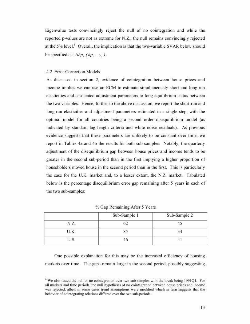
4.2 Error Correction Models

As discussed in section 2, evidence of cointegration between house prices and

income implies we can use an ECM to estimate simultaneously short and long-run

elasticities and associated adjustment parameters to long-equilibrium status between

the two variables. Hence, further to the above discussion, we report the short-run and

long-run elasticities and adjustment parameters estimated in a single step, with the

optimal model for all countries being a second order disequilibrium model (as

indicated by standard lag length criteria and white noise residuals). As previous

evidence suggests that these parameters are unlikely to be constant over time, we

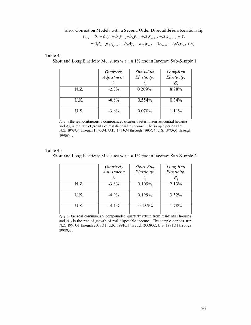
report in Tables 4a and 4b the results for both sub-samples. Notably, the quarterly

adjustment of the disequilibrium gap between house prices and income tends to be

greater in the second sub-period than in the first implying a higher proportion of

householders moved house in the second period than in the first. This is particularly

the case for the U.K. market and, to a lesser extent, the N.Z. market. Tabulated

below is the percentage disequilibrium error gap remaining after 5 years in each of

the two sub-samples:

% Gap Remaining After 5 Years

Sub-Sample 1 Sub-Sample 2

N.Z. 62 45

U.K. 85 34

U.S. 46 41

One possible explanation for this may be the increased efficiency of housing

markets over time. The gaps remain large in the second period, possibly suggesting

6 We also tested the null of no cointegration over two sub-samples with the break being 1991Q1. For

all markets and time periods, the null hypothesis of no cointegration between house prices and income

was rejected, albeit in some cases trend assumptions were modified which in turn suggests that the

behavior of cointegrating relations differed over the two sub-periods.

14

that although efficiency has increased it is by no means perfect. Further, the U.S.

results over the two sub-samples would indicate that this market is relatively more

efficient in reducing the disequilibrium error – a feature which may be related to the

fact that the U.S. market is a larger and more liquid market than its counterparts in the

U.K. and N.Z.

With the exception of the U.K. during the first sub-sample, long-run elasticities

tend to be higher than their short-run equivalents and indeed only the short-run

response for the U.K. is statistically significantly different from zero (not reported).

A possible explanation is the two-way interaction between credit availability and

housing prices which will increase the elasticity in the long run (Oikarinen, 2009b).

This is particularly noticeable for N.Z. during the first sub-sample where the long-run

response is particularly high at 8.8% and may be related to the regulatory regime in

operation in N.Z. at this time with effective access to mortgage finance being centrally

controlled.7 In general, however, the dominance of long-run elasticities is largely

consistent with the evidence from the literature which suggests first an under reaction

of prices (i.e., low short-run elasticities, then an overshooting after 1-4 years and

eventually convergence toward the long-run relationship (Harter-Dreiman, 2004;

Lamont and Stein, 1999; Capozza, Hendershott and Mack, 2004; Oikarinen, 2009a).

On the other hand, the results for the U.K. suggest that the relatively high short-run

elasticity reported for the first sub-sample may be related to the heavily discounted

sales of public housing stock to sitting tenants which generally could be financed on

very favorable terms. Long-run price responses to income were less for N.Z. in the

second time period, were greater for the U.K., while the U.S. exhibited a fairly stable

long-run response.

4.3 Structural VAR (SVAR)

We now turn to an analysis of the dynamic implications of the model by examining

the structural impulse response functions (IRFs) which, in Figures 1a through 1c,

picture the response of the level house prices to a (positive) one standard deviation

7 There was a ‘cap’ on mortgage finance in N.Z. during this period which is likely to have prevented

higher income being transmitted to house prices in the short-run but adjustment taking place in the

long-run. Fraser, Hoesli and McAlevey (2008a) also find that house prices and real income were out of

alignment during this period.

15

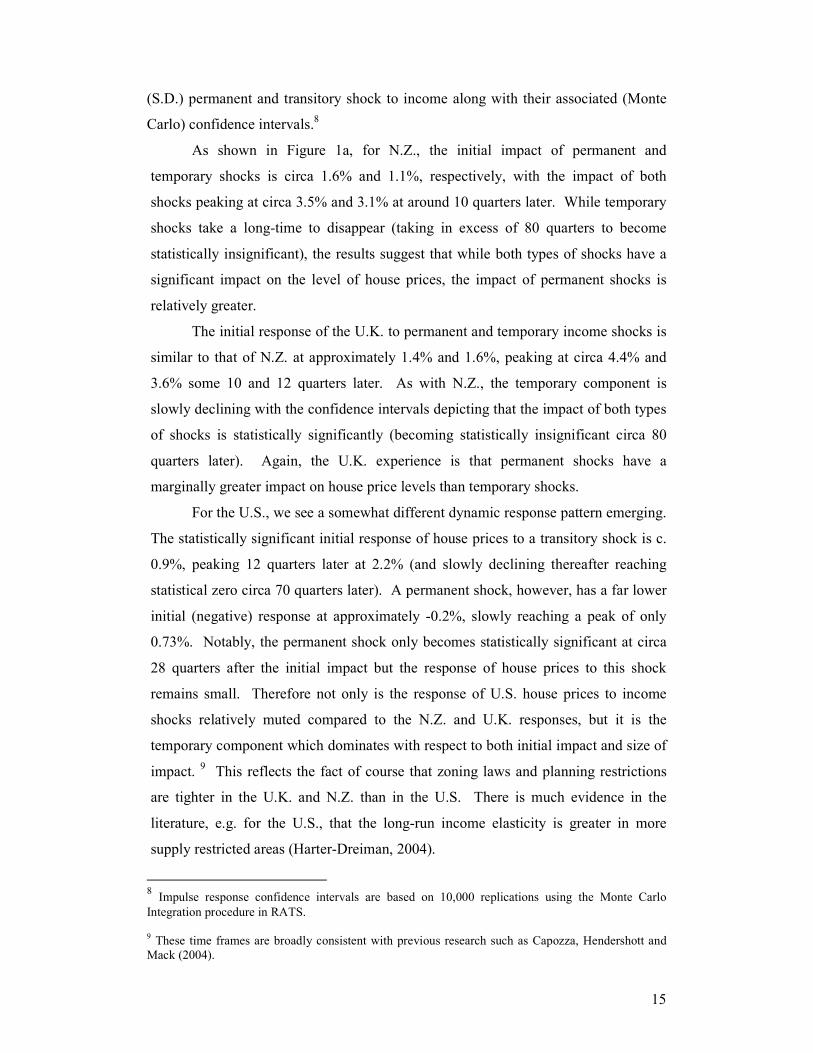
(S.D.) permanent and transitory shock to income along with their associated (Monte

Carlo) confidence intervals.8

As shown in Figure 1a, for N.Z., the initial impact of permanent and

temporary shocks is circa 1.6% and 1.1%, respectively, with the impact of both

shocks peaking at circa 3.5% and 3.1% at around 10 quarters later. While temporary

shocks take a long-time to disappear (taking in excess of 80 quarters to become

statistically insignificant), the results suggest that while both types of shocks have a

significant impact on the level of house prices, the impact of permanent shocks is

relatively greater.

The initial response of the U.K. to permanent and temporary income shocks is

similar to that of N.Z. at approximately 1.4% and 1.6%, peaking at circa 4.4% and

3.6% some 10 and 12 quarters later. As with N.Z., the temporary component is

slowly declining with the confidence intervals depicting that the impact of both types

of shocks is statistically significantly (becoming statistically insignificant circa 80

quarters later). Again, the U.K. experience is that permanent shocks have a

marginally greater impact on house price levels than temporary shocks.

For the U.S., we see a somewhat different dynamic response pattern emerging.

The statistically significant initial response of house prices to a transitory shock is c.

0.9%, peaking 12 quarters later at 2.2% (and slowly declining thereafter reaching

statistical zero circa 70 quarters later). A permanent shock, however, has a far lower

initial (negative) response at approximately -0.2%, slowly reaching a peak of only

0.73%. Notably, the permanent shock only becomes statistically significant at circa

28 quarters after the initial impact but the response of house prices to this shock

remains small. Therefore not only is the response of U.S. house prices to income

shocks relatively muted compared to the N.Z. and U.K. responses, but it is the

temporary component which dominates with respect to both initial impact and size of

impact. 9 This reflects the fact of course that zoning laws and planning restrictions

are tighter in the U.K. and N.Z. than in the U.S. There is much evidence in the

literature, e.g. for the U.S., that the long-run income elasticity is greater in more

supply restricted areas (Harter-Dreiman, 2004).

8 Impulse response confidence intervals are based on 10,000 replications using the Monte Carlo

Integration procedure in RATS. 9 These time frames are broadly consistent with previous research such as Capozza, Hendershott and

Mack (2004).

16

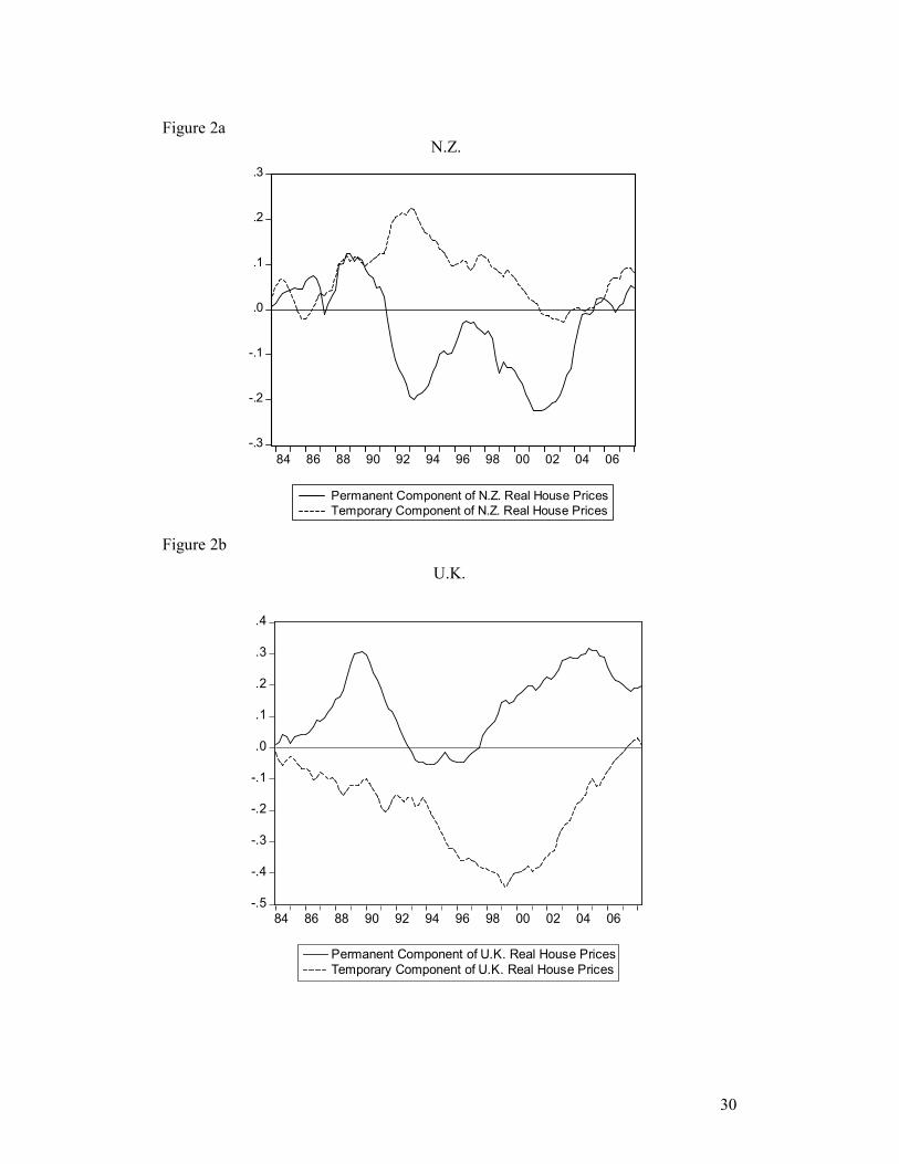
We can also decompose the house price series themselves into their permanent

and temporary components which enables us to compare and contrast the relative

importance of such components over time. Following from the discussion of the

SVAR in section 2, the permanent and temporary decompositions of the house price

series are shown in Figures 2a though 2c.

Clearly, permanent and temporary income disturbances have impacted on

N.Z., U.K. and U.S. house price movements in a different manner over the period. As

Figure 2a depicts, the N.Z. temporary component, unlike those of the U.K. and U.S.,

was predominantly positive over the period, peaking in 1993, falling sharply until late

2002 and rising again to 2007. In contrast, in the early 1990s, there was a sharp

negative change in the permanent component of house prices and the beginning of this

decline in the permanent component of prices occurs during the global recessionary

period of the early 1990s. Further, from the early 1990s through 1995, movements in

the temporary component tend to be negatively correlated with the permanent

component with the interaction between components keeping prices more stable than

they would otherwise have been. It would appear that over this period demand-type

influences did much to counteract the long-term influences on prices occurring in the

1990s.10 From 1996 to the end of the sample period, the permanent and temporary

components are positively correlated both falling until 2001 and rising thereafter.

The U.K. results provide quite a different picture of price behavior to that of

N.Z. Here it is the temporary component which is mainly negative over the period of

analysis, therefore dragging prices down with the permanent component mainly

positive. The exception to this is the period between late 1993 though 1997, where

both temporary and permanent components were negative, thus reinforcing the

dramatic fall in U.K. house prices over this period. Generally, in the U.K. the

temporary component has kept house prices lower than they would have been in the

absence of such shocks, although, as in N.Z., the latter part of the sample period has

seen permanent and temporary components reinforcing the upward trend in real

10 N.Z. has some unique characteristics in comparison with other OECD counties which may influence

the behavior of prices with respect to income shocks over the period. N.Z. households hold a

disproportionately high percentage of their assets in housing (Claus and Scobie, 2001) and by OECD,

standards have extremely low holdings of direct and indirect equities (Bollard, 2006). Perhaps it is no

surprise to find New Zealand to be different from the U.S. and U.K. Herring (2006, p. 8) quotes the

IMF (2006, p. 84) report: “global factors appear to explain about 70 percent of house price movements

in the United Kingdom and the United States, but only about 3 percent of house price movements in

New Zealand”. New Zealand is clearly an outlier.

17

prices. The permanent component began its recovery in the mid-1990s, somewhat

earlier than the temporary component but given the very negative effect of the

temporary component the overall result implies that house prices took a long time to

recover from this period of what is commonly called ‘negative equity’.

For the U.S., Figure 2c shows that from 1991 through 2002, the temporary

component of house prices was negative and although reinforced by the permanent

component had a much greater impact on price variability than the latter. Since 2002

and peaking in 2007, the temporary component has been well into the positive region.

Historically, however, and in contrast to the N.Z and U.K. housing market, the U.S.

market appears to be driven, by temporary rather than permanent shocks to income

and this is particularly noticeable in the period since 2000. The recent increases in the

temporary component may be explained by the impact of low interest rates and lax

credit conditions in force in this period of substantial economic growth and associated

real income rises. Figure 2c clearly indicates that since 2006 price decreases were to

be expected and that these decreases were driven by temporary components.

Figures 3a though 3c provide combination graphs with deterministic

components assigned to permanent components and graphed alongside temporary

components and demeaned (log) house price returns. For N.Z., particularly in the

1980s and 1990s and since 2005, actual prices tend to be higher than the permanent

and deterministic components combined would suggest with this deviation from long-

term trend being driven by the temporary component which was predominantly

positive over the period. This is in contrast with the results for the U.K. and the U.S.

but is consistent with results from other international studies. Fraser, Hoesli and

McAlevey (2008a), for example, report evidence to suggest that during the period

1988-2000, house prices in N.Z. were very close to their fundamental value as

warranted by (total) real disposable income. This suggests that the positive temporary

component of the prices series over this period had a role to play in the adjustment

process towards fundamental value and therefore accounts for the observed mean

reverting behavior of house price returns.

Over the period the upward movement in U.K. house prices can be seen to be

driven by the combined permanent and deterministic series but the rises moderated by

the temporary component which was mainly negative over the sample resulting in

actual prices lying below their long-term trend over much of the period. Figure 3c

shows that in the case of the U.S., the temporary component of prices also had a

18

moderating effect on long-term trend price rises until 2004 and a reinforcing effect

thereafter.

5. Conclusion

The aim of this paper is twofold. First, using time series analysis we specify the

nature of a two-variable system of house prices and income for N.Z., the U.K. and the

U.S., covering periods stretching from 1973:4 through 2008:2. Second, using an

SVAR econometric approach, the study distinguishes between the initial impact on

the levels of house prices of permanent and transitory shocks to the house

price−income system for each of the countries in the sample and continues by

decomposing historical house prices series into their permanent and transitory

components.

Our results suggest that for N.Z., the U.K. and the U.S., a long-run relationship

exists between house prices and income, although deviations from this stable

relationship are likely to occur. We also report evidence to suggest that while long-

run elasticities tend to dominate their short-run counterparts, they, along with the

adjustment parameters, are not constant over time. We maintain that this may arise

from the endogenous nature of house prices and income. Essentially, both house

prices and income are exposed to two types of macroeconomic shocks: permanent or

long-lasting shocks (e.g. supply-type disturbances) and temporary shocks (e.g.

demand-type disturbances) and while shocks which impinge on income are likely to

have much in common with those affecting house prices, the responsiveness of house

prices to income disturbances may differ according to whether they are viewed as

being of a permanent or transitory nature.

Utilizing an SVAR approach to house price–income relationships, we find that

for N.Z. the response of house prices to permanent and temporary shocks to income

was greater for the former although both types of shocks had a significant impact on

prices with the effects of temporary shocks only declining very slowly. The response

of U.K. house prices is similar to that of N.Z. in terms of magnitude and significance

while the response of the U.S., although relatively muted, is dominated by temporary

shocks with permanent shocks having no significant initial impact and very little

lasting impact on the level of U.S. house prices.

19

The method of analysis also allows us to decompose house prices into their

permanent and temporary components. For N.Z. over the period, actual prices tended

to be higher than the permanent and deterministic component alone would suggest

with this gap being driven by the temporary component which was mainly positive

over the period. This is in sharp contrast with the results for the U.K. and the U.S.

For the former, over the period the upward movement in house prices can be seen to

be driven by permanent and deterministic components of prices, with the rises being

moderated by the temporary component which was mainly negative. Our results also

show that in the case of the U.S. the temporary component dominates and, while the

permanent component provided some minor moderation of prices, since 2002 a major

driver of house prices has been the temporary or cyclical type influences impacting on

income.

Thus the evidence reported here suggests that there is no clear consistent

global pattern regarding the importance of permanent and temporary shocks to income

on house prices which implies that housing markets will react differently to the

vagaries of global and domestic economic activity driving such shocks – a feature

which should be considered in the wider context of international and domestic

macroeconomic policy decisions and implementation.

A number of caveats should be borne in mind when interpreting our findings.

First, the analysis was undertaken at a highly aggregate level and a more

disaggregated study examining the price behavior at regional levels (s.t. data

availability) might arrive at different conclusions. Second, as this work estimates a

bivariate model assigning the variations in house prices to income innovations, it

cannot specifically account for other types of innovations unrelated to the income

process. Future work may find it useful to consider for example, non-fundamental

shocks and the response of house prices to this third type of innovation thus providing

a clearer picture to emerge. Nevertheless, we feel that this paper can make a useful

contribution to our understanding of the behavior of house prices with respect to their

dynamic interaction with income in the markets analyzed.

20

References Banerjee, A., J.J. Dolado, D. F. Henry, and G.W. Smith (1986), ‘Exploring

Equilibrium Relationships in Econometrics Through Static Models: Some

Monte Carlo Evidence’, Oxford Bulletin of Economics and Statistics, 48, pp.

253-277.

Blanchard, O. J., and D. Quah (1989), ‘The Dynamic Effects of Demand and Supply

Disturbances’, American Economic Review, 79, pp. 655-673.

Bloch, H., P. Fraser and G. MacDonald (2009), ‘Commodity Prices: How Important

are Real and Nominal Shocks?’ Centre for Research in Applied Economics

Working Paper Series 200901. Bentley, Western Australia: Centre for

Research in Applied Economics, Curtin Business School: PUB-CBS-SEF-

MT-46728 Z3.

Bollard, A. (2006), ‘Kiwis Like Buying Houses More Than Buying Businesses’

Reserve Bank Governor’s Speech to Price-Waterhouse-Coopers Annual Tax

Conference, 9 November.

Bourassa, S.C., P. H. Hendershott and J. Murphy (2001), ‘Further Evidence on the

Existence of Housing Market Bubbles’, Journal of Property Research, 18, pp.

1-19.

Bourassa, S.C. and M. Hoesli (2010), ‘Why Do the Swiss Rent?’, Journal of Real

Estate Finance and Economics, forthcoming.

Campbell, J.Y. and R.J. Shiller (1989), ‘The Dividend-Price Ratio and Expectations

of Future Dividends and Discount factors’, Review of Financial Studies, 1, pp.

195-228.

Capozza, D.R, P.H. Hendershott and C. Mack (2004), ‘An Anatomy of Price

Dynamics in Illiquid Markets: Analysis and Evidence from Local Housing

Markets’, Real Estate Economics, 32, pp. 1-32.

Carroll, C.D. (2001), ‘Precautionary Saving and the Marginal Propensity to Consume

Out of Permanent Income’:

http://www.econ.jhu.edu/people/CCarroll/MPCPermBigNBER.pdf

Catte, P., N. Girouard, R. Price and C. André (2004), ‘The Contribution of Housing

Markets to Cyclical Resilience’, OECD Economic Studies No. 38.

Chan, H.L., S.K. Lee and K.Y. Woo (2001), ‘Detecting Rational Bubbles in the

Residential Housing Markets of Hong Kong’, Economic Modelling, 18, pp.

61-73.

Claus, I. and G. Scobie (2001), ‘Household Net Wealth: An International

Comparison’, New Zealand Treasury Working Paper, 01/19.

21

Clayton, J. (1996), ‘Rational Expectations, Market Fundamentals and Housing Price

Volatility’, Real Estate Economics, 24, pp. 441-470.

DiPasquale, D., and W. Wheaton (1994), ‘Housing Market Dynamics and the Future

of Housing Prices’, Journal of Urban Economics, 35, pp. 1-27.

Enders, W. (1995), Applied Econometric Time Series, John Wiley & Sons, Inc.

Engle, R.F. and C.W.J. Granger (1987), ‘Cointegration and Error Correction:

Representation, Estimation and Testing’, Econometrica, 55, pp. 251–276.

Fraser, P., M. Hoesli and L. McAlevey (2008a), ‘House Prices and Bubbles in New

Zealand’ Journal of Real Estate, Finance and Economics, 37, pp. 71-91.

Fraser, P., M. Hoesli and L. McAlevey (2008b), ‘A comparative analysis of house

prices and bubbles in the U.K. and New Zealand’ Pacific Rim Property

Research Journal, 14, pp. 257-278.

Gallin, J. (2006), ‘The Long-Run Relationship between House Prices and Income:

Evidence from Local Housing Markets’, Real Estate Economics, 34, pp. 417-

438.

Gonzalo, J. and C.W.J. Granger (1995), ‘Estimation of Common Long Memory

Components in Cointegrated Systems’, Journal of Business and Economics

Statistics, Vol. 13. pp. 27–35.

Goodhart, C. and B. Hofmann (2007), House Prices and the Macroeconomy:

Implications for Banking and Price Stability, Oxford University Press, Oxford.

Grimes, A., A. Aitken, I. Mitchell and V. Smith (2007), ‘Housing supply in the

Auckland region 2000-2005’, Centre for Housing Research, Wellington, New

Zealand.

Hannan, E. J. (1970), Multiple Time Series, Wiley, New York.

Harter-Dreiman, M. (2004), ‘Drawing Inferences About Housing Supply Elasticity

from House Price Responses to Income Shocks’, Journal of Urban

Economics, 55, pp. 316-337.

Herring, R.J. (2006), ‘Booms and Busts in Housing Markets: How Vulnerable is New

Zealand?’: http://www.rbnz.govt.nz/research/fellowship/3324563.pdf

Hess, P.J. and Lee, B-S. (1999), ‘Stock Returns and Inflation with Supply and

Demand Disturbances.’ The Review of Financial Studies, 12, pp. 1203-1218.

Holly, S. and N. Jones (1997), ‘House Prices since the 1940s: Cointegration,

Demography and Asymmetries’, Economic Modelling, 14, pp. 549-565.

22

Horioka, C.Y. (1988), ‘Tenure Choice and Housing Demand in Japan’ Journal of

Urban Economics, 24, pp. 258-309.

Hort, K. (1998), ‘The Determinants of Urban House Price Fluctuations in Sweden

1968-1994’, Journal of Housing Economics, 7, pp. 93-120.

Johansen, S. (1988), ‘Statistical Analysis of Cointegrating Vectors’, Journal of

Economic Dynamics and Control, 12, pp. 231-254.

IMF, (2006), World Economic Outlook, April, pp. 71-89.

Lamont, O. and J.C. Stein (1999), ‘Leverage and House-Price Dynamics in U.S.

Cities’, RAND Journal of Economics, 30, pp. 498-514.

Lee, B.-S. (1995), ‘The Response of Stock Prices to Permanent and Temporary

Dividend Shocks’, Journal of Financial and Quantitative Analysis, 30, pp. 1-

22.

Lee, T.H. (1968), ‘Housing and Permanent Income’, Review of Ecomometrics and

Statistics, 50, pp. 480-490.

Malpezzi, S. (1999), ‘A Simple Error Correction Model of House Prices’, Journal of

Housing Economics, 8, pp. 27-62.

Mayer, C. and R.G. Hubbard (2008), ‘House Prices, Interest Rates, and the Mortgage

Market Meltdown’, working paper, Columbia Business School.

Meen, G. (2002), ‘The Time-Series Behavior of House Prices: A Transatlantic

Divide?’, Journal of Housing Economics, 11, pp. 1-23.

Meese, R. and N. Wallace (2003), ‘House Price Dynamics and Market Fundamentals:

The Parisian Housing Market’, Urban Studies, 40, pp. 1027-1045.

Noord van den, P. (2006), ‘Are House Prices Nearing a Peak? A Probit Analysis of

17 OECD Countries’, OECD Economics Department Working Papers No.

488, 1 June 2006.

Oikarinen, E. (2009a), ‘Interaction Between Housing Prices and Household

Borrowing: The Finnish Case’, Journal of Banking and Finance, 33, pp. 747-

756.

Oikarinen, E. (2009b), ‘Household Borrowing and Metropolitan Housing Price

Dynamics – Empirical Evidence from Helsinki’, Journal of Housing

Economics, forthcoming.

Thomas , R.L. (1996), Modern Econometrics. Financial Times Prentice Hall.

Tse, R.Y.C. and J. Rafferty (1999), ‘Income Elasticity of Housing Consumption in

Hong-Kong: A Cointegration Approach.’ Journal of Property Research, 16:2,

pp. 123-138.

23

Table 1

Descriptive Statistics

Mean Standard

Deviation

Jarque-

Bera

(J-B)

N.Z. rhp,t

(real housing

returns)

0.023

0.026

15.563

(0.000)

N.Z. py,t

(real house price-

disposable income

ratio)

1.413

0.708

14.101

(0.001)

N.Z. ∆y,t

(real disposable

income growth)

0.006

0.012

18.511

(0.000)

U.K. rhp,t

(real housing

returns)

0.021

0.026

0.381

(0.827)

U.K. py,t

(real house price-

disposable income

ratio)

1.248

0.586

5.917

(0.052)

U.K. ∆y,t

(real disposable

income growth)

0.006

0.012

59.439

(0.000)

U.S. rhp,t

(real housing

returns)

0.014

0.011

0.309

(0.857)

U.S. py,t

(real house price-

disposable income

ratio)

0.526

0.226

2.733

(0.255)

U.S. ∆y,t

(real disposable

income growth)

0.008

0.098

24.345

(0.000)

rhp,t is the real continuously compounded quarterly return from residential

housing py,t is the constructed price-real disposable income ratio and ∆y,t is the

rate of growth of real disposable income. The sample periods are: N.Z. 1973Q4

through 2008Q1; U.K. 1973Q4 through 2008Q2; U.S. 1975Q1 through 2008Q2.

The figures in parenthesis below the J-B statistics are marginal significance

levels.

24

Table 2a

Correlations of Real House Prices and Real Disposable Income: Full Sample

N.Z.

corr ( rhp,t,, ∆y,t)

-0.008

(0.923)

U.K.


0.231

(0.006)

U.S.


0.082

(0.345) rhp,t is the continuously compounded quarterly return from residential housing, and ∆y,t is the rate

of growth of real disposable income. The sample periods are: N.Z. 1973Q4 through 2008Q1; U.K.

1973Q4 through 2008Q2; U.S. 1975Q1 through 2008Q2. The figures in parenthesis below the

correlations are marginal significance levels.

Table 2b

Correlations of Real House Prices and Real Disposable Income: Sub-Sample 1

N.Z.


-0.137

(0.264)

U.K.


0.272

(0.025)

U.S.


0.152

(0.234) rhp,t is the continuously compounded quarterly return from residential housing, and ∆y,t is the rate of

growth of real disposable income. The sample periods are: N.Z. 1973Q4: through 1990Q4; U.K.



Table 2c

Correlations of Real House Prices and Real Disposable Income: Sub-Sample 2

N.Z.


0.205

(0.090)

U.K.


0.209

(0.082)

U.S.


-0.009

(0.942) rhp,t is the continuously compounded quarterly return from residential housing, and ∆y,t is the rate of

growth of real disposable income. The sample periods are: N.Z. 1991Q1 through 2008Q1; U.K.



25

Table 3

Real House Price – Real Disposable Income Cointegration Tests

Johansen

Trace Test of

No

Cointegration

Johansen

Eigenvalue

Test of No

Cointegration

Model

Specification

and Lags

Interval in

First

Differences

N.Z. 23.986

cv: 20.262

prob: 0.014

21.774

cv: 15.892

prob: 0.005

Intercept, No

Trend

1-1

U.K. 36.189

cv: 20.262

prob: 0.000

29.464

cv: 15.892

prob: 0.000

Intercept, No

Trend

1-1

U.S. 73.543

cv: 20.261

prob: 0.000

65.080

cv:15.892

prob: 0.000

Intercept, No

Trend

1-1 cv denotes critical values and prob denotes p-values. In each case the null hypothesis

is that the variables are not cointegrated. The sample periods are: N.Z. 1973Q4

through 2008Q1; U.K. 1973Q4 through 2008Q2; U.S. 1975Q1 through 2008Q2.

26

Error Correction Models with a Second Order Disequilibrium Relationship

t2t,hp21t,hp12t31t2t10t,hp rrybybybbr εµµ ++++++= −−−−

t1t11,hp1t3t11t,hp2o yrybybr ελβλ∆∆µλβ ++−−+−= −−−−

Table 4a

Short and Long Elasticity Measures w.r.t. a 1% rise in Income: Sub-Sample 1

Quarterly

Adjustment:

λ

Short-Run

Elasticity:

1b

Long-Run

Elasticity:

1β

N.Z. -2.3% 0.209%

8.88%

U.K. -0.8% 0.554%

0.34%

U.S. -3.6% 0.070%

1.11%

rhp,t is the real continuously compounded quarterly return from residential housing

and ∆y,t is the rate of growth of real disposable income. The sample periods are:

N.Z. 1973Q4 through 1990Q4; U.K. 1973Q4 through 1990Q4; U.S. 1975Q1 through

1990Q4.

Table 4b

Short and Long Elasticity Measures w.r.t. a 1% rise in Income: Sub-Sample 2

Quarterly

Adjustment:

λ

Short-Run

Elasticity:

1b

Long-Run

Elasticity:

1β

N.Z. -3.8% 0.109%

2.13%

U.K. -4.9% 0.199%

3.32%

U.S. -4.1% -0.155%

1.78%

rhp,t is the real continuously compounded quarterly return from residential housing

and ∆y,t is the rate of growth of real disposable income. The sample periods are:

N.Z. 1991Q1 through 2008Q1; U.K. 1991Q1 through 2008Q2; U.S. 1991Q1 through

2008Q2.

27

Figure 1a

N.Z.

-.01

.00

.01

.02

.03

.04

5 10 15 20 25 30 35 40

Permanent Shock

Confidence Intervals

Response of N.Z. Real House Prices to a Permanent Shock

-.01

.00

.01

.02

.03

.04

5 10 15 20 25 30 35 40

Temporary Shock


Response Of N.Z. Real House Prices to a Temporary Shock

28

Figure 1b

U.K.

-.01

.00

.01

.02

.03

.04

.05

.06

5 10 15 20 25 30 35 40

Permanent Shock


Response of U.K. Real House Prices to a Permanent Shock

-.01

.00

.01

.02

.03

.04

.05

.06

5 10 15 20 25 30 35 40

Temporary Shock


Response of U.K. Real House Prices to a Temporary Shock

29

Figure 1c

U.S.

-.005

.000

.005

.010

.015

.020

.025

.030

5 10 15 20 25 30 35 40

Permanent Shock


Response of U.S. Real House Prices to a Permanent Shock

-.005

.000

.005

.010

.015

.020

.025

.030

5 10 15 20 25 30 35 40

Temporary Shock


Response of U.S. Real House Prices to a Temporary Shock

30

Figure 2a

N.Z.

-.3

-.2

-.1

.0

.1

.2

.3

84 86 88 90 92 94 96 98 00 02 04 06

Permanent Component of N.Z. Real House Prices

Temporary Component of N.Z. Real House Prices

Figure 2b

U.K.

-.5

-.4

-.3

-.2

-.1

.0

.1

.2

.3

.4

84 86 88 90 92 94 96 98 00 02 04 06

Permanent Component of U.K. Real House PricesTemporary Component of U.K. Real House Prices

31

Figure 2c

U.S.

-.12

-.08

-.04

.00

.04

.08

.12

.16

.20

86 88 90 92 94 96 98 00 02 04 06

Permanent Component of U.S. Real House Prices

Temporary Component of U.S. Real House Prices

32

Figure 3a

N.Z.

-.05

.00

.05

.10

.15

.20

.25

5.5

6.0

6.5

7.0

7.5

8.0

84 86 88 90 92 94 96 98 00 02 04 06

N.Z. (log) Real House Prices

Deterministic plus Permanent Component of N.Z. Real House Prices

Temporary Compnent of N.Z. Real House Prices

Figure 3b

U.K.

-.5

-.4

-.3

-.2

-.1

.0

.1

5.5

6.0

6.5

7.0

7.5

8.0

84 86 88 90 92 94 96 98 00 02 04 06

U.K. (log) Real House PricesDeterminisic Plus Permanent Component of U.K. Real House Prices

Temporary Component of U.K. Real House Prices

33

Figure 3c

U.S.

-.2

-.1

.0

.1

.2

5.2

5.6

6.0

6.4

6.8

86 88 90 92 94 96 98 00 02 04 06

U. S . (lo g ) R e a l H o u s e P ric e s De te rm in is tic p lu s P e rma n e n t C o mp o n e n t o f U. S . R e a l H o u se P ri ce sTe mp o ra ry C o mp o n e n t o f U. S . R e a l H o u se P ri c e s

McAlevey House Prices Disposable Income Permanent ...

Documents

Transcript of McAlevey House Prices Disposable Income Permanent ...