May Traffic Flow Fundamentals
474
-
Upload
fathurohman-ocimh -
Category
Documents
-
view
84 -
download
0
Transcript of May Traffic Flow Fundamentals

7/18/2019 May Traffic Flow Fundamentals
http://slidepdf.com/reader/full/may-traffic-flow-fundamentals 1/472

7/18/2019 May Traffic Flow Fundamentals
http://slidepdf.com/reader/full/may-traffic-flow-fundamentals 2/472

7/18/2019 May Traffic Flow Fundamentals
http://slidepdf.com/reader/full/may-traffic-flow-fundamentals 3/472

7/18/2019 May Traffic Flow Fundamentals
http://slidepdf.com/reader/full/may-traffic-flow-fundamentals 4/472
7/18/2019 May Traffic Flow Fundamentals
http://slidepdf.com/reader/full/may-traffic-flow-fundamentals 5/472

7/18/2019 May Traffic Flow Fundamentals
http://slidepdf.com/reader/full/may-traffic-flow-fundamentals 6/472

7/18/2019 May Traffic Flow Fundamentals
http://slidepdf.com/reader/full/may-traffic-flow-fundamentals 7/472

7/18/2019 May Traffic Flow Fundamentals
http://slidepdf.com/reader/full/may-traffic-flow-fundamentals 8/472

7/18/2019 May Traffic Flow Fundamentals
http://slidepdf.com/reader/full/may-traffic-flow-fundamentals 9/472

7/18/2019 May Traffic Flow Fundamentals
http://slidepdf.com/reader/full/may-traffic-flow-fundamentals 10/472

7/18/2019 May Traffic Flow Fundamentals
http://slidepdf.com/reader/full/may-traffic-flow-fundamentals 11/472

7/18/2019 May Traffic Flow Fundamentals
http://slidepdf.com/reader/full/may-traffic-flow-fundamentals 12/472
7/18/2019 May Traffic Flow Fundamentals
http://slidepdf.com/reader/full/may-traffic-flow-fundamentals 13/472

7/18/2019 May Traffic Flow Fundamentals
http://slidepdf.com/reader/full/may-traffic-flow-fundamentals 14/472

7/18/2019 May Traffic Flow Fundamentals
http://slidepdf.com/reader/full/may-traffic-flow-fundamentals 15/472

7/18/2019 May Traffic Flow Fundamentals
http://slidepdf.com/reader/full/may-traffic-flow-fundamentals 16/472

7/18/2019 May Traffic Flow Fundamentals
http://slidepdf.com/reader/full/may-traffic-flow-fundamentals 17/472

7/18/2019 May Traffic Flow Fundamentals
http://slidepdf.com/reader/full/may-traffic-flow-fundamentals 18/472
7/18/2019 May Traffic Flow Fundamentals
http://slidepdf.com/reader/full/may-traffic-flow-fundamentals 19/472

7/18/2019 May Traffic Flow Fundamentals
http://slidepdf.com/reader/full/may-traffic-flow-fundamentals 20/472

7/18/2019 May Traffic Flow Fundamentals
http://slidepdf.com/reader/full/may-traffic-flow-fundamentals 21/472

7/18/2019 May Traffic Flow Fundamentals
http://slidepdf.com/reader/full/may-traffic-flow-fundamentals 22/472

7/18/2019 May Traffic Flow Fundamentals
http://slidepdf.com/reader/full/may-traffic-flow-fundamentals 23/472

7/18/2019 May Traffic Flow Fundamentals
http://slidepdf.com/reader/full/may-traffic-flow-fundamentals 24/472
7/18/2019 May Traffic Flow Fundamentals
http://slidepdf.com/reader/full/may-traffic-flow-fundamentals 25/472

7/18/2019 May Traffic Flow Fundamentals
http://slidepdf.com/reader/full/may-traffic-flow-fundamentals 26/472

7/18/2019 May Traffic Flow Fundamentals
http://slidepdf.com/reader/full/may-traffic-flow-fundamentals 27/472

7/18/2019 May Traffic Flow Fundamentals
http://slidepdf.com/reader/full/may-traffic-flow-fundamentals 28/472

7/18/2019 May Traffic Flow Fundamentals
http://slidepdf.com/reader/full/may-traffic-flow-fundamentals 29/472

7/18/2019 May Traffic Flow Fundamentals
http://slidepdf.com/reader/full/may-traffic-flow-fundamentals 30/472

7/18/2019 May Traffic Flow Fundamentals
http://slidepdf.com/reader/full/may-traffic-flow-fundamentals 31/472

7/18/2019 May Traffic Flow Fundamentals
http://slidepdf.com/reader/full/may-traffic-flow-fundamentals 32/472

7/18/2019 May Traffic Flow Fundamentals
http://slidepdf.com/reader/full/may-traffic-flow-fundamentals 33/472

7/18/2019 May Traffic Flow Fundamentals
http://slidepdf.com/reader/full/may-traffic-flow-fundamentals 34/472

7/18/2019 May Traffic Flow Fundamentals
http://slidepdf.com/reader/full/may-traffic-flow-fundamentals 35/472

7/18/2019 May Traffic Flow Fundamentals
http://slidepdf.com/reader/full/may-traffic-flow-fundamentals 36/472

7/18/2019 May Traffic Flow Fundamentals
http://slidepdf.com/reader/full/may-traffic-flow-fundamentals 37/472
7/18/2019 May Traffic Flow Fundamentals
http://slidepdf.com/reader/full/may-traffic-flow-fundamentals 38/472

7/18/2019 May Traffic Flow Fundamentals
http://slidepdf.com/reader/full/may-traffic-flow-fundamentals 39/472

7/18/2019 May Traffic Flow Fundamentals
http://slidepdf.com/reader/full/may-traffic-flow-fundamentals 40/472
7/18/2019 May Traffic Flow Fundamentals
http://slidepdf.com/reader/full/may-traffic-flow-fundamentals 41/472

7/18/2019 May Traffic Flow Fundamentals
http://slidepdf.com/reader/full/may-traffic-flow-fundamentals 42/472

7/18/2019 May Traffic Flow Fundamentals
http://slidepdf.com/reader/full/may-traffic-flow-fundamentals 43/472

7/18/2019 May Traffic Flow Fundamentals
http://slidepdf.com/reader/full/may-traffic-flow-fundamentals 44/472

7/18/2019 May Traffic Flow Fundamentals
http://slidepdf.com/reader/full/may-traffic-flow-fundamentals 45/472

7/18/2019 May Traffic Flow Fundamentals
http://slidepdf.com/reader/full/may-traffic-flow-fundamentals 46/472

7/18/2019 May Traffic Flow Fundamentals
http://slidepdf.com/reader/full/may-traffic-flow-fundamentals 47/472

7/18/2019 May Traffic Flow Fundamentals
http://slidepdf.com/reader/full/may-traffic-flow-fundamentals 48/472

7/18/2019 May Traffic Flow Fundamentals
http://slidepdf.com/reader/full/may-traffic-flow-fundamentals 49/472

7/18/2019 May Traffic Flow Fundamentals
http://slidepdf.com/reader/full/may-traffic-flow-fundamentals 50/472

7/18/2019 May Traffic Flow Fundamentals
http://slidepdf.com/reader/full/may-traffic-flow-fundamentals 51/472

7/18/2019 May Traffic Flow Fundamentals
http://slidepdf.com/reader/full/may-traffic-flow-fundamentals 52/472

7/18/2019 May Traffic Flow Fundamentals
http://slidepdf.com/reader/full/may-traffic-flow-fundamentals 53/472

7/18/2019 May Traffic Flow Fundamentals
http://slidepdf.com/reader/full/may-traffic-flow-fundamentals 54/472

7/18/2019 May Traffic Flow Fundamentals
http://slidepdf.com/reader/full/may-traffic-flow-fundamentals 55/472

7/18/2019 May Traffic Flow Fundamentals
http://slidepdf.com/reader/full/may-traffic-flow-fundamentals 56/472

7/18/2019 May Traffic Flow Fundamentals
http://slidepdf.com/reader/full/may-traffic-flow-fundamentals 57/472

7/18/2019 May Traffic Flow Fundamentals
http://slidepdf.com/reader/full/may-traffic-flow-fundamentals 58/472

7/18/2019 May Traffic Flow Fundamentals
http://slidepdf.com/reader/full/may-traffic-flow-fundamentals 59/472

7/18/2019 May Traffic Flow Fundamentals
http://slidepdf.com/reader/full/may-traffic-flow-fundamentals 60/472

7/18/2019 May Traffic Flow Fundamentals
http://slidepdf.com/reader/full/may-traffic-flow-fundamentals 61/472

7/18/2019 May Traffic Flow Fundamentals
http://slidepdf.com/reader/full/may-traffic-flow-fundamentals 62/472
7/18/2019 May Traffic Flow Fundamentals
http://slidepdf.com/reader/full/may-traffic-flow-fundamentals 63/472

7/18/2019 May Traffic Flow Fundamentals
http://slidepdf.com/reader/full/may-traffic-flow-fundamentals 64/472

7/18/2019 May Traffic Flow Fundamentals
http://slidepdf.com/reader/full/may-traffic-flow-fundamentals 65/472

7/18/2019 May Traffic Flow Fundamentals
http://slidepdf.com/reader/full/may-traffic-flow-fundamentals 66/472
7/18/2019 May Traffic Flow Fundamentals
http://slidepdf.com/reader/full/may-traffic-flow-fundamentals 67/472

7/18/2019 May Traffic Flow Fundamentals
http://slidepdf.com/reader/full/may-traffic-flow-fundamentals 68/472

7/18/2019 May Traffic Flow Fundamentals
http://slidepdf.com/reader/full/may-traffic-flow-fundamentals 69/472

7/18/2019 May Traffic Flow Fundamentals
http://slidepdf.com/reader/full/may-traffic-flow-fundamentals 70/472

7/18/2019 May Traffic Flow Fundamentals
http://slidepdf.com/reader/full/may-traffic-flow-fundamentals 71/472
7/18/2019 May Traffic Flow Fundamentals
http://slidepdf.com/reader/full/may-traffic-flow-fundamentals 72/472

7/18/2019 May Traffic Flow Fundamentals
http://slidepdf.com/reader/full/may-traffic-flow-fundamentals 73/472

7/18/2019 May Traffic Flow Fundamentals
http://slidepdf.com/reader/full/may-traffic-flow-fundamentals 74/472

7/18/2019 May Traffic Flow Fundamentals
http://slidepdf.com/reader/full/may-traffic-flow-fundamentals 75/472

7/18/2019 May Traffic Flow Fundamentals
http://slidepdf.com/reader/full/may-traffic-flow-fundamentals 76/472
7/18/2019 May Traffic Flow Fundamentals
http://slidepdf.com/reader/full/may-traffic-flow-fundamentals 77/472

7/18/2019 May Traffic Flow Fundamentals
http://slidepdf.com/reader/full/may-traffic-flow-fundamentals 78/472

7/18/2019 May Traffic Flow Fundamentals
http://slidepdf.com/reader/full/may-traffic-flow-fundamentals 79/472

7/18/2019 May Traffic Flow Fundamentals
http://slidepdf.com/reader/full/may-traffic-flow-fundamentals 80/472

7/18/2019 May Traffic Flow Fundamentals
http://slidepdf.com/reader/full/may-traffic-flow-fundamentals 81/472

7/18/2019 May Traffic Flow Fundamentals
http://slidepdf.com/reader/full/may-traffic-flow-fundamentals 82/472

7/18/2019 May Traffic Flow Fundamentals
http://slidepdf.com/reader/full/may-traffic-flow-fundamentals 83/472

7/18/2019 May Traffic Flow Fundamentals
http://slidepdf.com/reader/full/may-traffic-flow-fundamentals 84/472

7/18/2019 May Traffic Flow Fundamentals
http://slidepdf.com/reader/full/may-traffic-flow-fundamentals 85/472

7/18/2019 May Traffic Flow Fundamentals
http://slidepdf.com/reader/full/may-traffic-flow-fundamentals 86/472

7/18/2019 May Traffic Flow Fundamentals
http://slidepdf.com/reader/full/may-traffic-flow-fundamentals 87/472

7/18/2019 May Traffic Flow Fundamentals
http://slidepdf.com/reader/full/may-traffic-flow-fundamentals 88/472

7/18/2019 May Traffic Flow Fundamentals
http://slidepdf.com/reader/full/may-traffic-flow-fundamentals 89/472

7/18/2019 May Traffic Flow Fundamentals
http://slidepdf.com/reader/full/may-traffic-flow-fundamentals 90/472

7/18/2019 May Traffic Flow Fundamentals
http://slidepdf.com/reader/full/may-traffic-flow-fundamentals 91/472

7/18/2019 May Traffic Flow Fundamentals
http://slidepdf.com/reader/full/may-traffic-flow-fundamentals 92/472

7/18/2019 May Traffic Flow Fundamentals
http://slidepdf.com/reader/full/may-traffic-flow-fundamentals 93/472

7/18/2019 May Traffic Flow Fundamentals
http://slidepdf.com/reader/full/may-traffic-flow-fundamentals 94/472
7/18/2019 May Traffic Flow Fundamentals
http://slidepdf.com/reader/full/may-traffic-flow-fundamentals 95/472

7/18/2019 May Traffic Flow Fundamentals
http://slidepdf.com/reader/full/may-traffic-flow-fundamentals 96/472

7/18/2019 May Traffic Flow Fundamentals
http://slidepdf.com/reader/full/may-traffic-flow-fundamentals 97/472

7/18/2019 May Traffic Flow Fundamentals
http://slidepdf.com/reader/full/may-traffic-flow-fundamentals 98/472

7/18/2019 May Traffic Flow Fundamentals
http://slidepdf.com/reader/full/may-traffic-flow-fundamentals 99/472

7/18/2019 May Traffic Flow Fundamentals
http://slidepdf.com/reader/full/may-traffic-flow-fundamentals 100/472

7/18/2019 May Traffic Flow Fundamentals
http://slidepdf.com/reader/full/may-traffic-flow-fundamentals 101/472

7/18/2019 May Traffic Flow Fundamentals
http://slidepdf.com/reader/full/may-traffic-flow-fundamentals 102/472

7/18/2019 May Traffic Flow Fundamentals
http://slidepdf.com/reader/full/may-traffic-flow-fundamentals 103/472

7/18/2019 May Traffic Flow Fundamentals
http://slidepdf.com/reader/full/may-traffic-flow-fundamentals 104/472

7/18/2019 May Traffic Flow Fundamentals
http://slidepdf.com/reader/full/may-traffic-flow-fundamentals 105/472
7/18/2019 May Traffic Flow Fundamentals
http://slidepdf.com/reader/full/may-traffic-flow-fundamentals 106/472

7/18/2019 May Traffic Flow Fundamentals
http://slidepdf.com/reader/full/may-traffic-flow-fundamentals 107/472
7/18/2019 May Traffic Flow Fundamentals
http://slidepdf.com/reader/full/may-traffic-flow-fundamentals 108/472

7/18/2019 May Traffic Flow Fundamentals
http://slidepdf.com/reader/full/may-traffic-flow-fundamentals 109/472

7/18/2019 May Traffic Flow Fundamentals
http://slidepdf.com/reader/full/may-traffic-flow-fundamentals 110/472

7/18/2019 May Traffic Flow Fundamentals
http://slidepdf.com/reader/full/may-traffic-flow-fundamentals 111/472

7/18/2019 May Traffic Flow Fundamentals
http://slidepdf.com/reader/full/may-traffic-flow-fundamentals 112/472
7/18/2019 May Traffic Flow Fundamentals
http://slidepdf.com/reader/full/may-traffic-flow-fundamentals 113/472

7/18/2019 May Traffic Flow Fundamentals
http://slidepdf.com/reader/full/may-traffic-flow-fundamentals 114/472

7/18/2019 May Traffic Flow Fundamentals
http://slidepdf.com/reader/full/may-traffic-flow-fundamentals 115/472

7/18/2019 May Traffic Flow Fundamentals
http://slidepdf.com/reader/full/may-traffic-flow-fundamentals 116/472

7/18/2019 May Traffic Flow Fundamentals
http://slidepdf.com/reader/full/may-traffic-flow-fundamentals 117/472
7/18/2019 May Traffic Flow Fundamentals
http://slidepdf.com/reader/full/may-traffic-flow-fundamentals 118/472

7/18/2019 May Traffic Flow Fundamentals
http://slidepdf.com/reader/full/may-traffic-flow-fundamentals 119/472

7/18/2019 May Traffic Flow Fundamentals
http://slidepdf.com/reader/full/may-traffic-flow-fundamentals 120/472

7/18/2019 May Traffic Flow Fundamentals
http://slidepdf.com/reader/full/may-traffic-flow-fundamentals 121/472

7/18/2019 May Traffic Flow Fundamentals
http://slidepdf.com/reader/full/may-traffic-flow-fundamentals 122/472

7/18/2019 May Traffic Flow Fundamentals
http://slidepdf.com/reader/full/may-traffic-flow-fundamentals 123/472

7/18/2019 May Traffic Flow Fundamentals
http://slidepdf.com/reader/full/may-traffic-flow-fundamentals 124/472

7/18/2019 May Traffic Flow Fundamentals
http://slidepdf.com/reader/full/may-traffic-flow-fundamentals 125/472

7/18/2019 May Traffic Flow Fundamentals
http://slidepdf.com/reader/full/may-traffic-flow-fundamentals 126/472

7/18/2019 May Traffic Flow Fundamentals
http://slidepdf.com/reader/full/may-traffic-flow-fundamentals 127/472

7/18/2019 May Traffic Flow Fundamentals
http://slidepdf.com/reader/full/may-traffic-flow-fundamentals 128/472

7/18/2019 May Traffic Flow Fundamentals
http://slidepdf.com/reader/full/may-traffic-flow-fundamentals 129/472

7/18/2019 May Traffic Flow Fundamentals
http://slidepdf.com/reader/full/may-traffic-flow-fundamentals 130/472

7/18/2019 May Traffic Flow Fundamentals
http://slidepdf.com/reader/full/may-traffic-flow-fundamentals 131/472

7/18/2019 May Traffic Flow Fundamentals
http://slidepdf.com/reader/full/may-traffic-flow-fundamentals 132/472

7/18/2019 May Traffic Flow Fundamentals
http://slidepdf.com/reader/full/may-traffic-flow-fundamentals 133/472

7/18/2019 May Traffic Flow Fundamentals
http://slidepdf.com/reader/full/may-traffic-flow-fundamentals 134/472

7/18/2019 May Traffic Flow Fundamentals
http://slidepdf.com/reader/full/may-traffic-flow-fundamentals 135/472

7/18/2019 May Traffic Flow Fundamentals
http://slidepdf.com/reader/full/may-traffic-flow-fundamentals 136/472

7/18/2019 May Traffic Flow Fundamentals
http://slidepdf.com/reader/full/may-traffic-flow-fundamentals 137/472

7/18/2019 May Traffic Flow Fundamentals
http://slidepdf.com/reader/full/may-traffic-flow-fundamentals 138/472

7/18/2019 May Traffic Flow Fundamentals
http://slidepdf.com/reader/full/may-traffic-flow-fundamentals 139/472

7/18/2019 May Traffic Flow Fundamentals
http://slidepdf.com/reader/full/may-traffic-flow-fundamentals 140/472

7/18/2019 May Traffic Flow Fundamentals
http://slidepdf.com/reader/full/may-traffic-flow-fundamentals 141/472

7/18/2019 May Traffic Flow Fundamentals
http://slidepdf.com/reader/full/may-traffic-flow-fundamentals 142/472

7/18/2019 May Traffic Flow Fundamentals
http://slidepdf.com/reader/full/may-traffic-flow-fundamentals 143/472
7/18/2019 May Traffic Flow Fundamentals
http://slidepdf.com/reader/full/may-traffic-flow-fundamentals 144/472

7/18/2019 May Traffic Flow Fundamentals
http://slidepdf.com/reader/full/may-traffic-flow-fundamentals 145/472

7/18/2019 May Traffic Flow Fundamentals
http://slidepdf.com/reader/full/may-traffic-flow-fundamentals 146/472

7/18/2019 May Traffic Flow Fundamentals
http://slidepdf.com/reader/full/may-traffic-flow-fundamentals 147/472

7/18/2019 May Traffic Flow Fundamentals
http://slidepdf.com/reader/full/may-traffic-flow-fundamentals 148/472

7/18/2019 May Traffic Flow Fundamentals
http://slidepdf.com/reader/full/may-traffic-flow-fundamentals 149/472
7/18/2019 May Traffic Flow Fundamentals
http://slidepdf.com/reader/full/may-traffic-flow-fundamentals 150/472

7/18/2019 May Traffic Flow Fundamentals
http://slidepdf.com/reader/full/may-traffic-flow-fundamentals 151/472

7/18/2019 May Traffic Flow Fundamentals
http://slidepdf.com/reader/full/may-traffic-flow-fundamentals 152/472

7/18/2019 May Traffic Flow Fundamentals
http://slidepdf.com/reader/full/may-traffic-flow-fundamentals 153/472

7/18/2019 May Traffic Flow Fundamentals
http://slidepdf.com/reader/full/may-traffic-flow-fundamentals 154/472

7/18/2019 May Traffic Flow Fundamentals
http://slidepdf.com/reader/full/may-traffic-flow-fundamentals 155/472
7/18/2019 May Traffic Flow Fundamentals
http://slidepdf.com/reader/full/may-traffic-flow-fundamentals 156/472

7/18/2019 May Traffic Flow Fundamentals
http://slidepdf.com/reader/full/may-traffic-flow-fundamentals 157/472
7/18/2019 May Traffic Flow Fundamentals
http://slidepdf.com/reader/full/may-traffic-flow-fundamentals 158/472
7/18/2019 May Traffic Flow Fundamentals
http://slidepdf.com/reader/full/may-traffic-flow-fundamentals 159/472

7/18/2019 May Traffic Flow Fundamentals
http://slidepdf.com/reader/full/may-traffic-flow-fundamentals 160/472

7/18/2019 May Traffic Flow Fundamentals
http://slidepdf.com/reader/full/may-traffic-flow-fundamentals 161/472
7/18/2019 May Traffic Flow Fundamentals
http://slidepdf.com/reader/full/may-traffic-flow-fundamentals 162/472

7/18/2019 May Traffic Flow Fundamentals
http://slidepdf.com/reader/full/may-traffic-flow-fundamentals 163/472
154 Macroscopic Speed Characteristics Chap. 5
5 5 SELECTED PROBLEMS
1. The traffic flow along an existing radial urban two-lane directional freeway in the peak
direction is 3000 vehicles per hour, which includes 5 percent recreational vehicles, 2 per
cent buses, and 10 percent trucks. The existing freeway has the following characteristics:
60-mile per hour design speed, 12-foot lanes, 8-foot shoulders on each side, and rolling ter
rain. The annual growth in traffic is increasing at a rate of 5 percent per year, with the
vehicle composition factors remaining about the same. Consideration is being given to
redesigning the freeway by adding a third lane, but because of right-of-way constraints, the
lane widths would be reduced to 11 feet, the left shoulder would be abandoned, and the
right shoulder would be reduced to 6 feet. The reconstruction is expected to take 3 years.
Estimate average speeds during this design hour under existing conditions, three years from
now with the existing design, and 3 years from now with the new design.
2. Conduct a library study of annual trends in freeway speeds for the period 1960 to the
present time. Assess the impact that the 55-mile per hour speed limit has had on average
speeds and speed distributions. Attempt to predict average speeds and speed distributions
when the speed limit was increased to 65 miles per hour on the rural freeway system.
3. Solve Problem 1 for the existing condition only. Estimate average speeds in each lane and
the average speed in the other direction during the same hour assuming a 60:40 directional
split in volume and the same vehicle mix.
4. Calculate the average two-way speed profile along the two-lane two-way rural highway
shown in Figure 5.6 using the 1985 Highway Capacity Manual The characteristics of the
highway and traffic situation are given below.
Geometric Characteristics
Road Type
Grade
Lane width ft)
Shoulder width (ft)
Design Speed (miles per hour)
Percent no-passing zones
Two-lane
3 ,5
12
6
60
50
Traffic Characteristics
Two-way volume (veh/hr)
Percent Trucks
PercentRVs
Directional split
600
5
5
50:50
Compare and assess differences between your calculations and the results shown in Figure
5.6.
5. The running or cruise speed of vehicles along an arterial is 30 miles per hour. There aresix signalized intersections along the arterial and are spaced 1/4 mile apart. You are to
make three estimates of the travel time from a point 1/4 mile upstream of the first signal to
just downstream of the stop line at the last signal. The three situations to be analyzed are
(a) theoretical minimum travel time at a constant speed of 30 miles per hour; (b) at night
time the signals are placed in flashing yellow operations along the arterial and vehicles
slow down to 20 miles per hour at each signalized intersection momentarily; and c) during
the time of day that signals are coordinated well for the opposite direction of traffic, the
traffic in one study direction is required to stop at every signal for an average of 20
seconds. Assume acceleration and deceleration rates considering values shown in Tables
4.2 and 4.4.

7/18/2019 May Traffic Flow Fundamentals
http://slidepdf.com/reader/full/may-traffic-flow-fundamentals 164/472

7/18/2019 May Traffic Flow Fundamentals
http://slidepdf.com/reader/full/may-traffic-flow-fundamentals 165/472

7/18/2019 May Traffic Flow Fundamentals
http://slidepdf.com/reader/full/may-traffic-flow-fundamentals 166/472

7/18/2019 May Traffic Flow Fundamentals
http://slidepdf.com/reader/full/may-traffic-flow-fundamentals 167/472

7/18/2019 May Traffic Flow Fundamentals
http://slidepdf.com/reader/full/may-traffic-flow-fundamentals 168/472

7/18/2019 May Traffic Flow Fundamentals
http://slidepdf.com/reader/full/may-traffic-flow-fundamentals 169/472

7/18/2019 May Traffic Flow Fundamentals
http://slidepdf.com/reader/full/may-traffic-flow-fundamentals 170/472

7/18/2019 May Traffic Flow Fundamentals
http://slidepdf.com/reader/full/may-traffic-flow-fundamentals 171/472

7/18/2019 May Traffic Flow Fundamentals
http://slidepdf.com/reader/full/may-traffic-flow-fundamentals 172/472

7/18/2019 May Traffic Flow Fundamentals
http://slidepdf.com/reader/full/may-traffic-flow-fundamentals 173/472

7/18/2019 May Traffic Flow Fundamentals
http://slidepdf.com/reader/full/may-traffic-flow-fundamentals 174/472

7/18/2019 May Traffic Flow Fundamentals
http://slidepdf.com/reader/full/may-traffic-flow-fundamentals 175/472

7/18/2019 May Traffic Flow Fundamentals
http://slidepdf.com/reader/full/may-traffic-flow-fundamentals 176/472

7/18/2019 May Traffic Flow Fundamentals
http://slidepdf.com/reader/full/may-traffic-flow-fundamentals 177/472

7/18/2019 May Traffic Flow Fundamentals
http://slidepdf.com/reader/full/may-traffic-flow-fundamentals 178/472

7/18/2019 May Traffic Flow Fundamentals
http://slidepdf.com/reader/full/may-traffic-flow-fundamentals 179/472

7/18/2019 May Traffic Flow Fundamentals
http://slidepdf.com/reader/full/may-traffic-flow-fundamentals 180/472

7/18/2019 May Traffic Flow Fundamentals
http://slidepdf.com/reader/full/may-traffic-flow-fundamentals 181/472
7/18/2019 May Traffic Flow Fundamentals
http://slidepdf.com/reader/full/may-traffic-flow-fundamentals 182/472

7/18/2019 May Traffic Flow Fundamentals
http://slidepdf.com/reader/full/may-traffic-flow-fundamentals 183/472
7/18/2019 May Traffic Flow Fundamentals
http://slidepdf.com/reader/full/may-traffic-flow-fundamentals 184/472

7/18/2019 May Traffic Flow Fundamentals
http://slidepdf.com/reader/full/may-traffic-flow-fundamentals 185/472

7/18/2019 May Traffic Flow Fundamentals
http://slidepdf.com/reader/full/may-traffic-flow-fundamentals 186/472

7/18/2019 May Traffic Flow Fundamentals
http://slidepdf.com/reader/full/may-traffic-flow-fundamentals 187/472

7/18/2019 May Traffic Flow Fundamentals
http://slidepdf.com/reader/full/may-traffic-flow-fundamentals 188/472

7/18/2019 May Traffic Flow Fundamentals
http://slidepdf.com/reader/full/may-traffic-flow-fundamentals 189/472

7/18/2019 May Traffic Flow Fundamentals
http://slidepdf.com/reader/full/may-traffic-flow-fundamentals 190/472

7/18/2019 May Traffic Flow Fundamentals
http://slidepdf.com/reader/full/may-traffic-flow-fundamentals 191/472

7/18/2019 May Traffic Flow Fundamentals
http://slidepdf.com/reader/full/may-traffic-flow-fundamentals 192/472

7/18/2019 May Traffic Flow Fundamentals
http://slidepdf.com/reader/full/may-traffic-flow-fundamentals 193/472

7/18/2019 May Traffic Flow Fundamentals
http://slidepdf.com/reader/full/may-traffic-flow-fundamentals 194/472
7/18/2019 May Traffic Flow Fundamentals
http://slidepdf.com/reader/full/may-traffic-flow-fundamentals 195/472

7/18/2019 May Traffic Flow Fundamentals
http://slidepdf.com/reader/full/may-traffic-flow-fundamentals 196/472

7/18/2019 May Traffic Flow Fundamentals
http://slidepdf.com/reader/full/may-traffic-flow-fundamentals 197/472

7/18/2019 May Traffic Flow Fundamentals
http://slidepdf.com/reader/full/may-traffic-flow-fundamentals 198/472

7/18/2019 May Traffic Flow Fundamentals
http://slidepdf.com/reader/full/may-traffic-flow-fundamentals 199/472

7/18/2019 May Traffic Flow Fundamentals
http://slidepdf.com/reader/full/may-traffic-flow-fundamentals 200/472

7/18/2019 May Traffic Flow Fundamentals
http://slidepdf.com/reader/full/may-traffic-flow-fundamentals 201/472

7/18/2019 May Traffic Flow Fundamentals
http://slidepdf.com/reader/full/may-traffic-flow-fundamentals 202/472

7/18/2019 May Traffic Flow Fundamentals
http://slidepdf.com/reader/full/may-traffic-flow-fundamentals 203/472

7/18/2019 May Traffic Flow Fundamentals
http://slidepdf.com/reader/full/may-traffic-flow-fundamentals 204/472

7/18/2019 May Traffic Flow Fundamentals
http://slidepdf.com/reader/full/may-traffic-flow-fundamentals 205/472
7/18/2019 May Traffic Flow Fundamentals
http://slidepdf.com/reader/full/may-traffic-flow-fundamentals 206/472

7/18/2019 May Traffic Flow Fundamentals
http://slidepdf.com/reader/full/may-traffic-flow-fundamentals 207/472

7/18/2019 May Traffic Flow Fundamentals
http://slidepdf.com/reader/full/may-traffic-flow-fundamentals 208/472

7/18/2019 May Traffic Flow Fundamentals
http://slidepdf.com/reader/full/may-traffic-flow-fundamentals 209/472

7/18/2019 May Traffic Flow Fundamentals
http://slidepdf.com/reader/full/may-traffic-flow-fundamentals 210/472

7/18/2019 May Traffic Flow Fundamentals
http://slidepdf.com/reader/full/may-traffic-flow-fundamentals 211/472

7/18/2019 May Traffic Flow Fundamentals
http://slidepdf.com/reader/full/may-traffic-flow-fundamentals 212/472

7/18/2019 May Traffic Flow Fundamentals
http://slidepdf.com/reader/full/may-traffic-flow-fundamentals 213/472

7/18/2019 May Traffic Flow Fundamentals
http://slidepdf.com/reader/full/may-traffic-flow-fundamentals 214/472
StationNo.SM
Distancesmiles)
7:00
7:30
' 8:00Ei
8:30
9:00
9:30
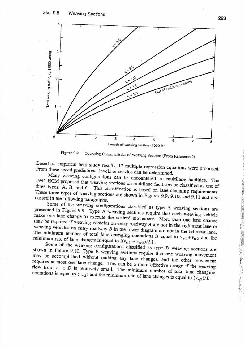
Sec. 7.4 Introduction to Shock Waves. 2 5
system-wide density contour maps have been developed from aerial photographic stu
dies. An example of each is shown in Figures 7.4, 7.5, and 7.6. The application of
density contour maps as an i n t r ~ d u t i o n to shock waves, and for estimating travel time
.and traffic demands are addressed in the following three sections of this chapter.
0 > 5% occupancy Eilll15-25% occupancy MkN < 15% occupancy
igure 7.4 Percent Occupancy Contour Map from Santa Monica Freeway Surveillance System
7 4 INTRODUCTION TO SHOCK WAVES
The purpose of this section is to .provide a qualitative introduction to shock wave
analysis. ·Quantitative analysis of shock waves will be covered in later sections of thischapter -and in Chapter 11. Shock waves are defined as boundary •conditions in the
time-space domain that demark a discontinuity in flow-density conditions. For purposes
of this 9-iscussion, the distinct discontinuity between noncongested and congested flow
will be considered, and a density contour of 60 vehicles per lane-mile will be used to
identify this discontinuity. This single type of shock wave is considered here because
of its importance and in order to present the concept of shock waves as clearly and con
cisely as possible. In Chapter 11 the approach to shock wave analysis is generalized.
In the following paragraphs two simple traffic situations are presented and then a matrix
of more complex traffic situations is presented and discussed. ·
.
i l

7/18/2019 May Traffic Flow Fundamentals
http://slidepdf.com/reader/full/may-traffic-flow-fundamentals 215/472

7/18/2019 May Traffic Flow Fundamentals
http://slidepdf.com/reader/full/may-traffic-flow-fundamentals 216/472

7/18/2019 May Traffic Flow Fundamentals
http://slidepdf.com/reader/full/may-traffic-flow-fundamentals 217/472
JL
t
'
'
i:
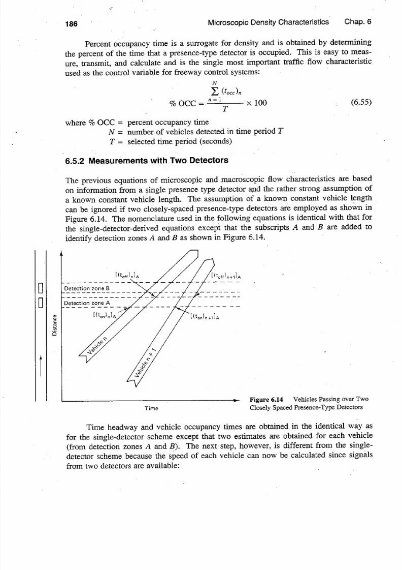
2 8 Macroscopic Density Characteristics Chap. 7
7 4 1 Some Simple Examples
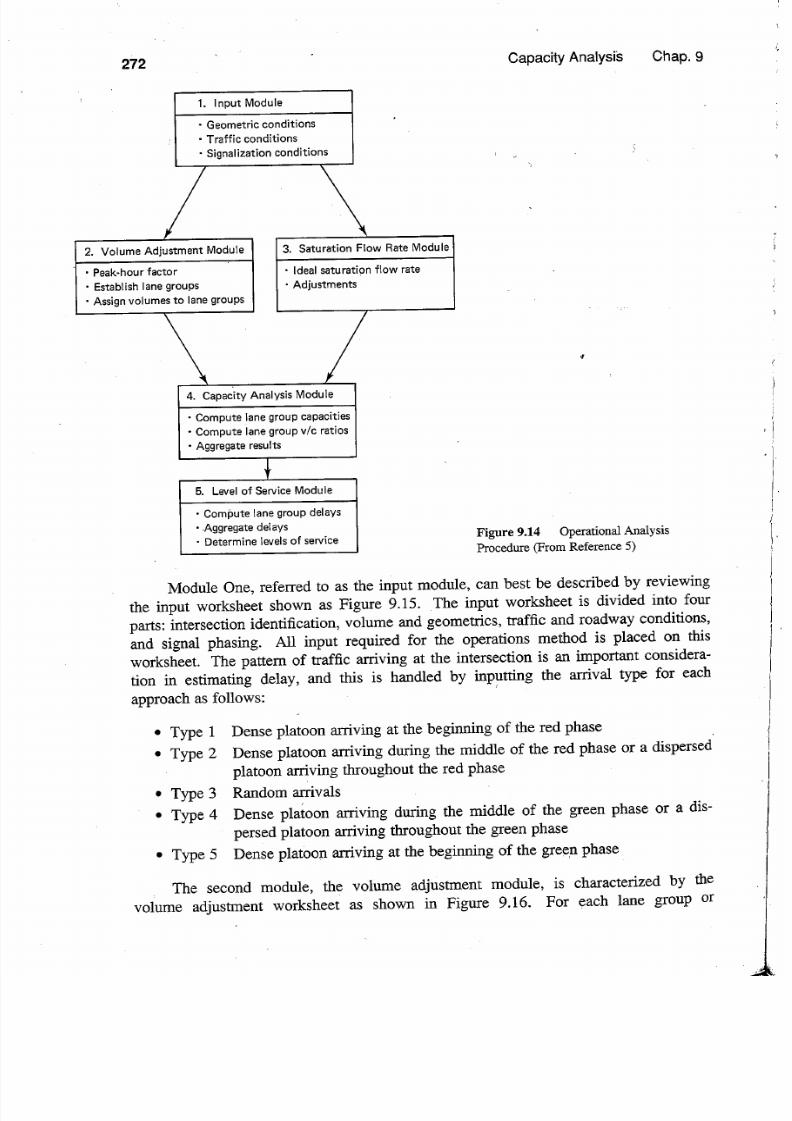
Consider a single-lane approach to a pretimed signal-controlled intersection as shown in
Figure 7.7. The traffic demand is assumed to be relatively light and arriving at a con
stant flow rate. The capacity o the traffic signal exceeds the arriving traffic demand but
traffic can only be discharged when the signal is green. Consequently, at some distance
upstream of the signal and immediately downstream of the signal, free-flow conditions
exist with densities less than 60 vehicles per lane-mile. However, just upstream o the
signal during the red phase, vehicles will be stopped and densities will exceed 60 vehi
cles per lane-mile. Therefore, ther.e will be a discontinuity as vehicles join the rear of
the standing queue and as vehicles are discharged from the front of the standing queue
when the signal is green. The first discontinuity is a backward forming shock wave
while the second discontinuity is a backward recovery shock wave. Both shock waves
are backward moving because over time the discontinuity is propagating upstream in theopposite direction of the moving traffic. The first shock wave is a forming shock wave
because over time the propagation of the shock wave is resulting in the increase of the
congested portion while the second shock wave is a recovery shock wave because over
time the propagation of the shock wave is resulting in the decrease of the congested
portion. There is a frontal stationary shock wave at the stop line during the red phase.
The term frontal is used to indicate that the shock wave is at the downstream edge of
the congested region, and the term stationary is used to indicate that the shock wave
remains at the same position in space. Consider this example as the case where demand
is constant over time, capacity varies over time, and there is an isolated single restric
tion (bottleneck) with no entrances or exits in the congested region.
Frontal
stationary
shock wave
Backwardforming
shock wave
Green
ime
ed
Backwardrecovery
shock wave
Figure 7.7 Shock Wave Phenomena at a
Signalized Intersection

7/18/2019 May Traffic Flow Fundamentals
http://slidepdf.com/reader/full/may-traffic-flow-fundamentals 218/472
t tIII I
I II II II II II II III
t t tI II I
Sec. 7.4 Introduction to Shock Waves 2 9
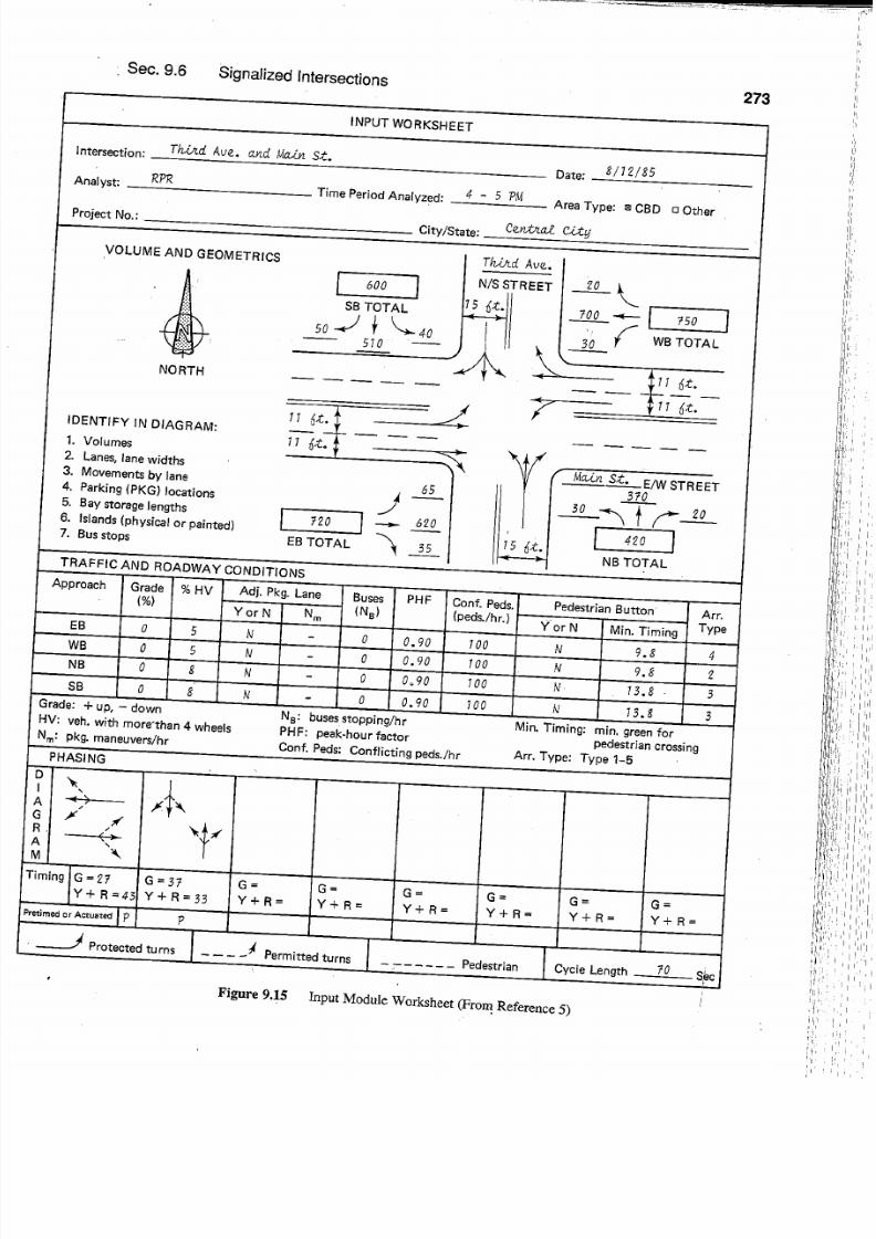
The second simple traffic situation is at a lane-drop location on a long bridge dur
ing the afternoon peak period and is shown in Figure 7.8. The capacity of the lane-drop
·location is constant over time, but like the typical peak period the traffic demands
· increase, causing demands to exceed capacities and then decrease until the peak period
is over. For illustrative purposes the demand flow over time pattern will be assumed to
be equivalent to 1.5 2.5, 2.0, and 1.5 lanes of capacity note that the bottleneck capa
city is 2 lanes). During the first period of time when demand is equivalent to 1.5 lanes
o capacity, no shock wave contour of 60 vehicles per lane-mile) will develop. How
ever, as soon as the demand increases to 2.5 lanes of capacity, a backward-forming
shock wave will develop having a constant shock wave velocity. When the demand is
reduced to 2 Janes of capacity, the input equals the output and a rear stationary shock
wave resUlts. As the demand is reduced further to 1.5 lanes of capacity, the length o
the congestion region decreases, as shown by the forward recovery shock wave. A
frontal stationary shock wave occurs at the bottleneck as long as the bottleneck operatesat capacity. The intersection of the frontal stationary shock wave and the forward
recovery shock wave signifies the termination of the congested period. Consider this
example as the case where demand varies over time, the capacity is fixed, and there is
an isolated single restriction with no entrances or exits in the congested region.
':
i:S
Bottlenecklocation
Backwardforming
shock wave
Time
Frontalstationary
shock wave
Rear
stationaryshock wave
Forwardrecovery
shock wave
Figure 7.8 Shock Wave Phenomena at a
Freeway Bottleneck during a Peak Period.
Traffic situations in the real world are usually much more complex than the two
examples described in the previous paragraphs. Consider the major assumptions that
were implicitly made or implied in order to develop a matrix of more typical real-world
situations. These assumptions include:
• An isolated bottleneck
II
' '

7/18/2019 May Traffic Flow Fundamentals
http://slidepdf.com/reader/full/may-traffic-flow-fundamentals 219/472
210 Macroscopic Density Characteristics Chap. 7
• A constant demand (or capaCity) over time
• A varying demand capacity} over time of a simplistic nature
• Normal conditions free of incidents, accidents, and so on
• No forward-moving forming shock wave (as shown in Figure 7.3 between Bronson and Cahuenga at 4:35 to 4:40P.M.)
• No entrances or exits along the route
7 4 2 Further Examples and Classification
An attempt will now be made to classify the different types of shock waves and to
describe situations where and when they might be encountered. Before doing so, a
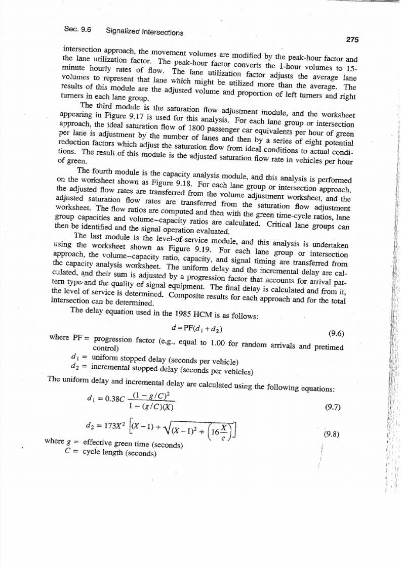
hypothetical and complex density contour map will be presented (Figure 7.9) and the
resulting shock waves described. The vertical scale of Figure 7.9 is distance, with
traffic moving up the diagram, and six locations are identified in the figure and
described below:
I e
1: G gII @jI
.
IItl @-1 I { :\II \.SI
llIII
Q
"i5
tltit0-lII
A Farthest downstream recurring bottleneck
B Nonrecurring incident site
C Second recurring bottleneck
D Location where demand dropped at time 9
E Third recurring bottleneck
F Upstream end of congestion
·
Time
k<6o Dk>6o I I
Figure 7.9 Hypothetical Density Contour
Map
7/18/2019 May Traffic Flow Fundamentals
http://slidepdf.com/reader/full/may-traffic-flow-fundamentals 220/472
Sec. 7.4 Introduction to Shock Waves 2
The horizontal scale is time, with time increasing to the right. A total of 15 points in
time are identified in the figure and will be described as the example is presented. The
clear _area in the time-space domain indicates areas where densities are less than 60
vehicles per lane-mile, while the shaded area indicates where densities are greater than
60 vehicles per lane-mile. The boundaries between these two areas illustrate almost all
of the various 'types of shock waves that can exist.
At time 5, the first congestion is encountered at location C causing a frontal sta
tionary shock wave 5-6) and a backward forming shock wave (5-9). At time 10
congestion occurs at. location E causing a frontal stationary shock wave (10-11), a
backward forming shock wave (10-14), and reduces the velocity of the backward form
ing shoc;k wave 9-1 1). At time 6 trucks in the congestion upstream of location C are
slowed down, and as the trucks proceed along the upgrade, their speeds are inhibited
n ~ a forward forming shock wave resulted (6-1). Location becomes the bottleneck
and a newfrontal stationary shock wave is created (1-2). At time 3 an incident occursat location B that causes a forward recovery shock wave 2-3) and establishes a new
frontal stationary shock wave (3-4). At time 4, the i )cident at location B is removed
and a backward recovery shock wave is formed (4-7). At time 7 the bottleneck at
location C is reestablished and a frontal stationary shock wave is formed (7-8). The
congested length "splits" at time 12, forming a new frorital stationary shock wave
(12-13) and lowers the demands between locations E and C creating a forward
recovery shock wave (12-8). Returning to point 14 the demand decreases until the
input demand is equal to the flow in the congested region which causes a rear stationary
shock wave (14-15). Further reduction in input demand causes a forward recovery
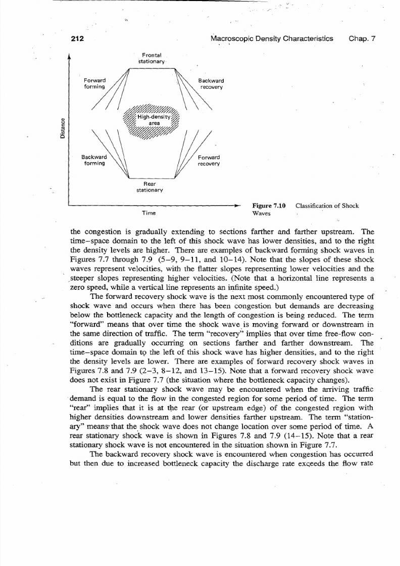
shock wave (15-13). The congestion ends at time 13.In summarizing this introduction to shock waves, Figure 7.10 attempts to classify
the various types of shock waves and relate this classification to the earlier examples
given in Figures 7.7 through,7.9. The six types of shock waves are identified in Figure
7.10. The high-density area (densities > 60 vehicles per lane-mile) is shown in the
center of the figure, while low densities (densities< 60 vehicles per mile) are located on
the outside of the individual shock waves. A frontal stationary shock wave must always
be present at a bottleneck location and indicates the location where traffic demand
exceeds capacity. It may be due to recurrent situations where each workday the normal
demands exceed normal capacities during the peak period at specific locations or be due
to nonrecurrent situations where the normal demand exceeds reduced capacity (caused
by accident or incident) which may occur at any location at any time. The term "fron
tal" implies that it is at the front (or downstream edge) of the congested region with
-lower densities farther downstream and higher densities upstream. The term "station
ary" means that the shock wave is fixed by location; that is, it does not change location
over time. There are examples of frontal stationary shock waves in Figures 7.7 through
7.9 1-2, 3-4, 5-6, 7-8, 10-11, and 12-13).
Backward forming shock waves must always be present if congestion occurs and
indicates the area in the time-space domain where excess demands are being stored.
The term "backward" means that over time the shock wave is moving backward orupstream in the opposite direction of traffic. The term "forming" implies that over ~ i m
I
I
I
I
7/18/2019 May Traffic Flow Fundamentals
http://slidepdf.com/reader/full/may-traffic-flow-fundamentals 221/472
Q)
t0
2 2Frontal
stationary
Rearstationary
Time
Macroscopic Density Characteristics Chap. 7
Figure 7.10 Classification of Shock
Waves
the congestion is gradually extending to sections farther and farther upstream. The
time-space domain to the left of this shock wave has lower densities, and to the right
the density levels are higher. There are examples of backward forming shock waves in
Figures 7.7 through 7.9 5-9, 9-11, and 10-14). Note thatthe slopes of these shock
waves represent velocities, with the flatter slopes representing lower velocities and the· steeper slopes representing higher velocities. (Note that a horizontal line represents a
zero speed, while a vertical line represents an infinite speed.)
The forward recovery shock wave is the next most commonly encountered type of
shock wave and occurs when there has been congestion but demands are decreasing
below the bottleneck capacity and the length of congestion is being reduced. The term
forward means that over time the shock wave. is moving forward or downstream in
the same direction of traffic. The term recovery implies that over time free-flow con
ditions are gradually occurring on sections farther and farther downstream. The
time-space domain t9 the left of this shock wave has higher densities, and to the right
the density levels are lower. There are examples of forward recovery shock waves inFigures 7.8 and 7.9 2-3, 8-12, and 13-15). Note that a forward recovery shock wave
does not exist in Figure 7.7 (the situation where the bottleneck capacity changes).
The rear stationary shock wave may be encountered when the arriving traffic
demand is equal to the flow in the congested region for some period of time. The term
rear implies that it is at th e rear (or upstream edge) of the congested region with
higher densities downstream and lower densities farther upstream. The term station
ary means· that the. shock wave does not change location over some period of time. A
rear stationary shock wave is shown in Figures 7.8 and 7.9 (14-15). Note that a rear
stationary shock wave is not encountered in the situation shown in Figure 7.7.
The backward recovery shock wave is encountered when congestion has occurred
but then due to increased bottleneck capacity the discharge rate exc;eeds the flow rate

7/18/2019 May Traffic Flow Fundamentals
http://slidepdf.com/reader/full/may-traffic-flow-fundamentals 222/472
Sec 7 5 Estimating Total Travel Time 213
within the congested region. The term backward means that over time the shock
wave is moving backward or upstream in the opposite direction o traffic. The term
recovery implies that over time free-flow conditions are extending farther and farther
upstream from the previous bottleneck location. The congested region is to the left o
the shock wave and free-flow conditions are·to the right. There are examples o backward recovery waves in Figures 7.7 and 7.9 (4-7). Note that a backward recovery
shock wave is not encountered in the situation shown in Figure 7.8.
. The last type of shock wave is the forward forming shock wave. This type o
shdck wave is not too common. The term forward implies that the shock wave
moves ip the same direction as traffic, and '.'forming means that over time the conges
tion is gradually extending to sections farther and farther downstream. The time-space
domain to the left o this shock wave has lower densities, and to the right, the density
levels are higher. A forward forming shock wave is shown in Figure 7.9 (6-1). Note
that a forward forming shock wave is not encountered iri Figure 7.7 or 7.8.
The purpose o this section was to introduce briefly the subject o shock waves.The reader should be aware that this is only an introduction, for only the most important
elements o shock waves are presented in a qualitative manner with strong assumptions.
There are other types o waves to be considered in addition to shock waves. Shock
waves demark all discontinuities in flow-density conditions not just at a density discon
tinuity o a specific density level such as 60 vehicles per lane-mile. Finally, many
assumptions were made in order to enhance the simplicity and clarity o the presenta
tion. The reader is referred to Chapter 11 for further discussion and analysis o shock
waves.
7 5 ESTIMATING TOTAL TRAVEL TIME
The total travel time (TTT) expended in a system during a selected time period can be
estimated by determining the average number o vehicles in the system and multiplying
by the length o the time period.
TTT V·T (7.12)
where TTT = total travel time expended in the system during the selected time period
(vehicle-hours) ·V = average number o vehicles in the system during the selected time period
= time period o observations (hours)
The average number o vehicles in the system can be estimated by determining the
number of vehicles in the system at frequent intervals during the time period selected.
mLVV ~m
where m = number o observations during the time period selectedvr = number o vehicles irrthe system at time t
(7.13) il

7/18/2019 May Traffic Flow Fundamentals
http://slidepdf.com/reader/full/may-traffic-flow-fundamentals 223/472
214 Macroscopic Density Characteristics Chap 7
The number of vehicles in the system at time interval t can be estimated by knowing the
densities, lengths, and number of lanes in each subsection of the system, and then sum
ming over all subsections in the system:
where n = number of subsections in the system
kit = density in subsection i at time t (vehicles per lane-mile)
Li = length of subsection i (miles)
Ni = number of lanes in subsection i
(7.14)
Substituting equation (7.14) into equation (7.13) and in turn, into equation (7.12), the
total travel time expended in a system during a time period T can be estimated from the
following equation.
(7.15)
Consider a situation on a 3.8 mile section of directional freeway during the afternoon
peak period. The freeway section is divided into seven subsections and the afternoon
peak period from 3:45 until 6:30 P.M. is divided into eleven 15-minute time periods. A
density contour map is available and the density kit in vehicles per lane-mile) is deter
mined for ea,.ch cell (subsection i during time period t), as shown in Table 7.2. Given
·the subsection length and number of lanes for each subsection i the number of vehiclesin each subsection and time period vu) can be calculated as shown in Table 7.2. The
number of vehicles in the system at observation period t vt) is obtained as the sum of
the vertical vit values and are shown in Table 7.2 in the bottom row. The average
number of vehicles in the system V during the selection time period is shown in Table
7.2 in the bottom right cell and found to be 813.2 vehicles. The total travel time
expended in the system during the selected time period (3:45 to 6:30P.M.) is estimated
to be 2236.3 vehicle-hours using equation (7.12).
7 6 ESTIMATING TRAFFIC DEMAND
Traffic demand rate is defined as the number of vehicles that currently wish t pass a
point or short section in a given period of time and normally is expressed as a rate of
flow in vehicles per hour. Traffic demand does not include latent demand, but only the
demand that currently uses the transportation system. f the traffic demand rates at vari
ous points in the system do not exceed their corresponding capacities, all vehicles that
currently wish to pass can be accommodated, and the measured flow rate in the field is
the traffic demand rate. However, if traffic demand rates exceed their corresponding
capacities, the measured ~ w rates in the congested sections and downstream sections
represent the number of vehicles (per unit of time) that can be handled, not the number

7/18/2019 May Traffic Flow Fundamentals
http://slidepdf.com/reader/full/may-traffic-flow-fundamentals 224/472
1\
01
T BLE 7 2 Estimating Total Travel Time.
Subsection Length Number 15-Minute Time Interval Ending at:•
Number, of Lanes, of Lanes,
i Li i 4:00 4:15 4:30 4:45 5:00 5:15 5:30
I Alvarado 0.39 4 35 34 42 38 48 51 61
to 54.6 53.0 65.5 59.3 74.9 79.6 95.2
Rampart
2 Ramprut 0.50 4 39 38 59 52 44 72 71
to 78.0 76.0 Il8.0 104.0 88.0 144.0 142.0
Silver Lake
3 Silver Lake 0.58 4 32 40 39 47 49 66 75
to 74.2 92.8 90.5 109.0 113.7 153 1 174.0
Vermont
4 Vermont 0.64 4 24 29 29 40 60 67 73
to 61.4 74.2 74.2 102.4 153.6 171.5 186.9
Normandie
5 Norman die 0.83 4 29 26 48 82 82 88 93
to 96.3 86.3 159.4 272.2 272.2 292.2 308.8
Western
6 Western 0.47 4 36 47 62 79 81 95 79
to 67.7 88.4 II6.6 148.5 152.3 178.6 148.5
Sunset
7 Sunset 0.39 3 40 61 86 80 85 100 90.
to 46.8 71.4 100.6 93.6 99.4 117.0 105.3
Hollywood
All v Alvadaro 3.8 3 479,0 542.1 724.8 889.0 954.1 1136.0 II60.7
to and
Hollywood 4
•The first value given is the average density in vehicles per lane-mile; the second value is the average total
number of vehicles in the subsection.
Source Reference 24 .
5:45
44
68.6
34
68.0
63
146.2
66
169.0
95
315.4
91
17l.l
85
99.4
1037.7
6:00 6:15 6:30 l it
27 30 28
42.1 46.8 43.7 683.3
27 28 32
54.0 56.0 64.0 992.0
50 24 32
116.0 55.7 74.2 1199.4
68 26 21
174 1 66.6 53.8 1287.7
85 64 22
282.2 212.5 . 73.0 2370.5
78 79 29
146.6 148.5 54.5 1421.3
96 75 49
112.3 87.8 57.3 990.9
927.3 673.9 420.5 813.2
v
7/18/2019 May Traffic Flow Fundamentals
http://slidepdf.com/reader/full/may-traffic-flow-fundamentals 225/472
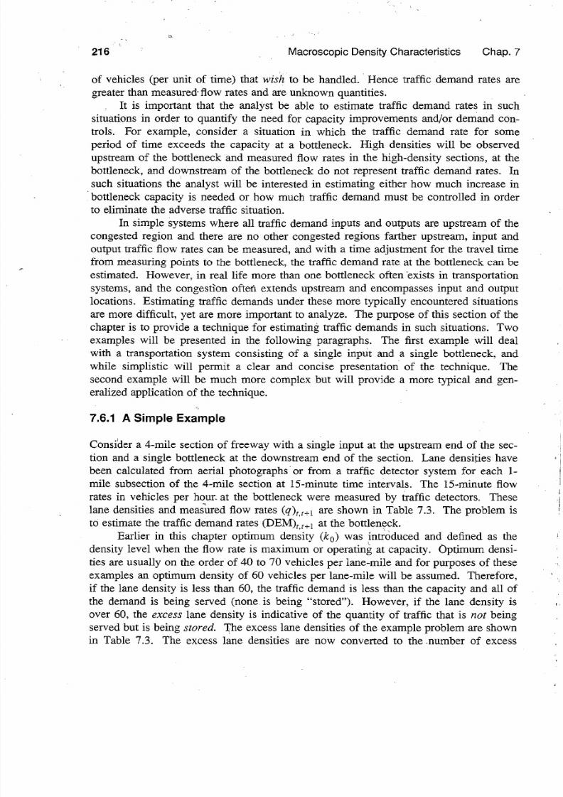
216 Macroscopic Density Characteristics Chap. 7
of vehicles (per unit of time) that wish to be handled. Hence traffic demand rates are
greater than measured· flow rates and are unknown quantities.
It is important that the analyst be able to estimate traffic demand rates in such
situations in order to quantify the need for capacity improvements and/or demand con
trols. For example, consider a situation in which the traffic demand rate for some
period of time exceeds the capacity at a bottleneck. High densities will be observed
upstream of the bottleneck and measured flow rates in the high-density sections, at the
bottleneck, and downstream of the bottleneck do not represent traffic demand rates. In
such situations the analyst will be interested in estimating either how much increase in
· bottleneck capacity is needed or how much traffic demand must be controlled in order
to eliminate the adverse traffic situation.
In simple systems where all traffic demand inputs and outputs are upstream of the
congested region and there are no other congested regions farther upstream, input and
output traffic flow rates can be measured, and with a time adjustment for the travel timefrom measuring points to the bottleneck, the traffic demand rate at the bottleneck can be
estimated. However, in real life more than one bottleneck often ·exists in transportation
systems, and the congestion oftefi extends upstream and encompasses input and output
locations. Estimating traffic demands under these more typically encountered situations
are more difficult, yet are more important to analyze. The purpose of this section of the
chapter is to provide a technique for estimating traffic demands in such situations. Two
examples will be presented in the following paragraphs. The first example will deal
with a transportation system consisting of a single input and a single bottleneck, and
while simplistic will permit a clear and concise presentation of the technique. The
second example will be much more complex but will provide a more typical and generalized application of the technique.
7 6 1 A Simple Example
Consi'der a 4-mile section of freeway with a single input at the upstream end of the sec
tion and a single bottleneck at the downstream end of the section. Lane densities have
been calculated from aerial photographs or from a traffic detector system for each 1-
mile subsection of the 4-mile section at 15-minute time intervals. The 15-minute flow
rates in vehicles per hour. at the bottleneck were measured by traffic detectors. These
lane densities and meas ured flow rates q)t,t+l are shown in Table 7.3. The problem is
to estimate the traffic demand rates (DEM)1 t l at the bottleneck.
Earlier in this chapter optimum e n ~ i t y (k 0 was introduced and defined as thel .
density level when the flow rate is maximum or operating at capacity. Optimum densi-
ties are usually on the order of 40 to 70 vehicles per lane-mile and for purposes of these
examples an optimum density of 60 vehicles per lane-mile will be assumed. Therefore,
if the lane density is less than 60, the traffic demand is less than the capacity and all of
the demand is being served (none. is being stored ). However, if the lane density is
over 60, the excess lane density is indicative of the quantity of traffic that is not being
served but is being stored. 'I(he excess lane densities of the example problem are shownin Table 7.3. The excess lane densities are now converted to the .number of excess

7/18/2019 May Traffic Flow Fundamentals
http://slidepdf.com/reader/full/may-traffic-flow-fundamentals 226/472

7/18/2019 May Traffic Flow Fundamentals
http://slidepdf.com/reader/full/may-traffic-flow-fundamentals 227/472

7/18/2019 May Traffic Flow Fundamentals
http://slidepdf.com/reader/full/may-traffic-flow-fundamentals 228/472

7/18/2019 May Traffic Flow Fundamentals
http://slidepdf.com/reader/full/may-traffic-flow-fundamentals 229/472

7/18/2019 May Traffic Flow Fundamentals
http://slidepdf.com/reader/full/may-traffic-flow-fundamentals 230/472

7/18/2019 May Traffic Flow Fundamentals
http://slidepdf.com/reader/full/may-traffic-flow-fundamentals 231/472

7/18/2019 May Traffic Flow Fundamentals
http://slidepdf.com/reader/full/may-traffic-flow-fundamentals 232/472
Chap 7 Selected roblems 223
4:00 to 5:30P.M.) and is negative demand rates less than capacity) from time interval 8
through time interval 11 5:30 to 6:30 P.M.). The measured flow rate and estimated
demand rate are shown in the upper portion o the illustration, and the shaded area
denotes differences between flows and demands.
It should be noted that while congestion e g ~ n s in time interval 2 and extends into
time interval 11, the demand rate exceeds the capacity only from time interval 2 throughtime interval 7. The congestion from time interval 8 through time interval 11 is not due
to demand rates exceeding capacities during this period o time but to unsatisfied
demands during earlier time intervals being transferred to this period of time. Capacity
increases at the bottleneck on the order o 400 vehicles per hour 7 to 8 percent) would
eliminate the congestion under the current estimated demand pattern. However, such an
improvement would cause some temporal and spatial driver responses which would
modify the demand pattern and thereby affect the full benefits of the improvement.
Controlling the input demand to the bottleneck would be another possible approach to
reducing congestion. The unserved flow rate gives an indication of the time period
needed for demand control and the magnitude of the diversion.
7 7 SELECTED PROBLEMS
1 The use of density as a macroscopic traffic flow characteristic has increased significantly
during the past 20 to 30 years. Review the 1950, 1965, and 1985 Highway apacity
Manuals to observe this increased use o density.
2. The metering rate at local traffic-responsive ramp signals are determined on-line as a func
tiono
percent occupancy measured on the freeway. Plot metering rateas
a functiono
percent occupancy graphically based on a review o freeway entry control literature. Con
sider maximum and minimum metering rate limits.
3. Develop an equation for the speed-density relationship shown in Figure 7.1. What would
be. the resulting numerical values for optimum density, jam density, and capacity? Also
determine the resulting speeds when flow i4 near zero and when the flow is i capacity.
4 Derive the equation for density as a function o percent occupancy without the use of the
text.
5. Assuming a reasonable relationship between speed and density, convert the density contour
map shown in Figure 7.3 to a speed contour map. Give particular attention to the regions
around the 40 and60
density contour lines.6. Interpret the percent occupancy contour map shown in Figure 7.4 with particular attention
to the identification of bottlenecks and shock waves.
7. Interpret the density contour map shown in Figure 7.5 with particular attention to the
identification of bottlenecks and shock waves.
8. Identify the bottlenecks and assess the severity o congested locations as shown in Figure
7.6 o the San Francisco Bay Area Freeway System.
9. Design and conduct a field experiment that will demonstrate the typical shock wave
phenomena o a single lane at a signalized intersection see Figure 7.7).
10 Assume that the field experiment described in Problem 9 is undertaken at a signalized
intersection having a 90-second cycle with 67 percent effective green time. The backward

7/18/2019 May Traffic Flow Fundamentals
http://slidepdf.com/reader/full/may-traffic-flow-fundamentals 233/472
224 Macroscopic Density Characteristics Chap 7
forming and backward recovery shock waves are found to be 4 and 10 miles per hour,
respectively. How far upstream of the stop line will the stopped queue of vehicles extend?
Is this approach oversaturated? What effect would that have on the maximum stopped
queue distance?
11 Congestion is observed at ·a freeway bottleneck location from 7:00 until 9:00 A.M.. Max
imum queueing extends 2 miles upstream and is observed at 8:15A.M . Assuming no rearstationary shock wave, identify and calculate the velocities of all other shock waves.
12. Draw a hypothetical density contour map that includes all types of shoc;k waves and
describe the traffic flow situations.
13. Estimate the total travel time for the situation presented in Table 7.3.
14 Estimate the total delay time per lane during one cycle of the traffic signal described in
Problem 10. Assume a density of 200 vehicles per lane-mile in the stopped queue and a
constant arrival rate of vehicles. What proportion of the vehicles will have to stop?
15 Estimate the total travel time in the congestion upstream of the freeway bottleneck
described in Problem 11. Assume an average density of 80 vehicles per lane-mile in the
congested region.
16 Estimate the traffic demand at the bottleneck for the problem described in Table 7:3, except
use an optimum density value of 50 rather than 60 vehicles per lane-mile. Plot results
similar to Figure 7 11.
17. Estimate the traffic demand at the bottleneck for the problem described in Table 7.4, except
use. an optimum density value of 70 rather than 60 vehicles per lane-mile. Plot results
similar to Figure 7.12. ·
18 In the closing paragraph of Section 7.6.2 a capacity increase at the bottleneck on the order
·of 400 vehicles per hour was recognized as needed to eliminate the congestion under the
current estimated demand pattern. Then an alert was given that this improvement might
modify the temporal and spatial patterns of traffic and affect the full benefits of the
improvement. Explain. Would controlling the input demand have the same effect?
7 8 SELECTED REFERENCES
1. Wolfgang S. Homburger and James H. Kell, Fundamentals of Traffic Engineering University
of California, Berkeley, Calif. 1988, pages 4-6 to 4-7.
2. Institute of Transportation Engineers, Transportation and Traffic Engineering Handbook 2nd
Edition, Prentice-Hall, Inc., Englewood Cliffs, N.J. 1982, pages 472-473 and 533-534.
3. Martin Wohl and Brian V. Martin, Traffic System Analysis for Engineers and Planners
McGraw-Hill Book Company, New York, 1967, pages 322-329 and 391-395.
4. Daniel L. Gerlough and Matthew J. Huber, Traffic Flow Theory A Monograph Transporta
tion Research Board, Special Report 165, TRB, Washington D. C., 1975, pages 10-12.
5. Bruce D. Greenshields, The Density Factor in Traffic Flow, Traffic Engineering Vol. 30, No.
6, March 1960, pages 26-28 and 30.
6. Frank A Haight, The Volume Density Relation in Theory of Road Traffic, Operations
Research _ Vol. 8, No.4 July-August 1960, pages 512-573.
7. John J. Haynes, The Development of the Use of Vehicular Density as a Control Element for
Freeway Operations Ph.D. Dissertation, Texas A M University, August 1964, 162 pages.

7/18/2019 May Traffic Flow Fundamentals
http://slidepdf.com/reader/full/may-traffic-flow-fundamentals 234/472

7/18/2019 May Traffic Flow Fundamentals
http://slidepdf.com/reader/full/may-traffic-flow-fundamentals 235/472

7/18/2019 May Traffic Flow Fundamentals
http://slidepdf.com/reader/full/may-traffic-flow-fundamentals 236/472

7/18/2019 May Traffic Flow Fundamentals
http://slidepdf.com/reader/full/may-traffic-flow-fundamentals 237/472

7/18/2019 May Traffic Flow Fundamentals
http://slidepdf.com/reader/full/may-traffic-flow-fundamentals 238/472
7/18/2019 May Traffic Flow Fundamentals
http://slidepdf.com/reader/full/may-traffic-flow-fundamentals 239/472

7/18/2019 May Traffic Flow Fundamentals
http://slidepdf.com/reader/full/may-traffic-flow-fundamentals 240/472

7/18/2019 May Traffic Flow Fundamentals
http://slidepdf.com/reader/full/may-traffic-flow-fundamentals 241/472
7/18/2019 May Traffic Flow Fundamentals
http://slidepdf.com/reader/full/may-traffic-flow-fundamentals 242/472

7/18/2019 May Traffic Flow Fundamentals
http://slidepdf.com/reader/full/may-traffic-flow-fundamentals 243/472

7/18/2019 May Traffic Flow Fundamentals
http://slidepdf.com/reader/full/may-traffic-flow-fundamentals 244/472

7/18/2019 May Traffic Flow Fundamentals
http://slidepdf.com/reader/full/may-traffic-flow-fundamentals 245/472

7/18/2019 May Traffic Flow Fundamentals
http://slidepdf.com/reader/full/may-traffic-flow-fundamentals 246/472

7/18/2019 May Traffic Flow Fundamentals
http://slidepdf.com/reader/full/may-traffic-flow-fundamentals 247/472

7/18/2019 May Traffic Flow Fundamentals
http://slidepdf.com/reader/full/may-traffic-flow-fundamentals 248/472

7/18/2019 May Traffic Flow Fundamentals
http://slidepdf.com/reader/full/may-traffic-flow-fundamentals 249/472

7/18/2019 May Traffic Flow Fundamentals
http://slidepdf.com/reader/full/may-traffic-flow-fundamentals 250/472

7/18/2019 May Traffic Flow Fundamentals
http://slidepdf.com/reader/full/may-traffic-flow-fundamentals 251/472

7/18/2019 May Traffic Flow Fundamentals
http://slidepdf.com/reader/full/may-traffic-flow-fundamentals 252/472

7/18/2019 May Traffic Flow Fundamentals
http://slidepdf.com/reader/full/may-traffic-flow-fundamentals 253/472

7/18/2019 May Traffic Flow Fundamentals
http://slidepdf.com/reader/full/may-traffic-flow-fundamentals 254/472
7/18/2019 May Traffic Flow Fundamentals
http://slidepdf.com/reader/full/may-traffic-flow-fundamentals 255/472

7/18/2019 May Traffic Flow Fundamentals
http://slidepdf.com/reader/full/may-traffic-flow-fundamentals 256/472

7/18/2019 May Traffic Flow Fundamentals
http://slidepdf.com/reader/full/may-traffic-flow-fundamentals 257/472

7/18/2019 May Traffic Flow Fundamentals
http://slidepdf.com/reader/full/may-traffic-flow-fundamentals 258/472

7/18/2019 May Traffic Flow Fundamentals
http://slidepdf.com/reader/full/may-traffic-flow-fundamentals 259/472

7/18/2019 May Traffic Flow Fundamentals
http://slidepdf.com/reader/full/may-traffic-flow-fundamentals 260/472

7/18/2019 May Traffic Flow Fundamentals
http://slidepdf.com/reader/full/may-traffic-flow-fundamentals 261/472

7/18/2019 May Traffic Flow Fundamentals
http://slidepdf.com/reader/full/may-traffic-flow-fundamentals 262/472

7/18/2019 May Traffic Flow Fundamentals
http://slidepdf.com/reader/full/may-traffic-flow-fundamentals 263/472

7/18/2019 May Traffic Flow Fundamentals
http://slidepdf.com/reader/full/may-traffic-flow-fundamentals 264/472

7/18/2019 May Traffic Flow Fundamentals
http://slidepdf.com/reader/full/may-traffic-flow-fundamentals 265/472

7/18/2019 May Traffic Flow Fundamentals
http://slidepdf.com/reader/full/may-traffic-flow-fundamentals 266/472

7/18/2019 May Traffic Flow Fundamentals
http://slidepdf.com/reader/full/may-traffic-flow-fundamentals 267/472

7/18/2019 May Traffic Flow Fundamentals
http://slidepdf.com/reader/full/may-traffic-flow-fundamentals 268/472

7/18/2019 May Traffic Flow Fundamentals
http://slidepdf.com/reader/full/may-traffic-flow-fundamentals 269/472

7/18/2019 May Traffic Flow Fundamentals
http://slidepdf.com/reader/full/may-traffic-flow-fundamentals 270/472

7/18/2019 May Traffic Flow Fundamentals
http://slidepdf.com/reader/full/may-traffic-flow-fundamentals 271/472
7/18/2019 May Traffic Flow Fundamentals
http://slidepdf.com/reader/full/may-traffic-flow-fundamentals 272/472

7/18/2019 May Traffic Flow Fundamentals
http://slidepdf.com/reader/full/may-traffic-flow-fundamentals 273/472

7/18/2019 May Traffic Flow Fundamentals
http://slidepdf.com/reader/full/may-traffic-flow-fundamentals 274/472

7/18/2019 May Traffic Flow Fundamentals
http://slidepdf.com/reader/full/may-traffic-flow-fundamentals 275/472

7/18/2019 May Traffic Flow Fundamentals
http://slidepdf.com/reader/full/may-traffic-flow-fundamentals 276/472

7/18/2019 May Traffic Flow Fundamentals
http://slidepdf.com/reader/full/may-traffic-flow-fundamentals 277/472

7/18/2019 May Traffic Flow Fundamentals
http://slidepdf.com/reader/full/may-traffic-flow-fundamentals 278/472

7/18/2019 May Traffic Flow Fundamentals
http://slidepdf.com/reader/full/may-traffic-flow-fundamentals 279/472

7/18/2019 May Traffic Flow Fundamentals
http://slidepdf.com/reader/full/may-traffic-flow-fundamentals 280/472
7/18/2019 May Traffic Flow Fundamentals
http://slidepdf.com/reader/full/may-traffic-flow-fundamentals 281/472
7/18/2019 May Traffic Flow Fundamentals
http://slidepdf.com/reader/full/may-traffic-flow-fundamentals 282/472

7/18/2019 May Traffic Flow Fundamentals
http://slidepdf.com/reader/full/may-traffic-flow-fundamentals 283/472
7/18/2019 May Traffic Flow Fundamentals
http://slidepdf.com/reader/full/may-traffic-flow-fundamentals 284/472

7/18/2019 May Traffic Flow Fundamentals
http://slidepdf.com/reader/full/may-traffic-flow-fundamentals 285/472

7/18/2019 May Traffic Flow Fundamentals
http://slidepdf.com/reader/full/may-traffic-flow-fundamentals 286/472
7/18/2019 May Traffic Flow Fundamentals
http://slidepdf.com/reader/full/may-traffic-flow-fundamentals 287/472

7/18/2019 May Traffic Flow Fundamentals
http://slidepdf.com/reader/full/may-traffic-flow-fundamentals 288/472
Chap 9 Selected Problems
c = capacity of lane group (vehicles per hour)
= volume-capacity ratio for the lane group
79
The level of service is determined based only on the average stopped delay per
vehicle in the following manner:
• Delays less than 5 seconds LOS A
• Delays 5 15 seconds
• Delays 15 25 seconds
• Delays 25 40 seconds
.. Delays 40 60 seconds
• Delays > 60 seconds
9 7 SUMMARY
LOS B
LOSC
LOSD
LOSE
LOSF
This chapter serves as an introduction to analytical techniques for capacity and level of
service determination of critical elements of the highway system. Heavy emphasis has
been placed on the 1985 Highway Capacity Manual and for more comprehensive and
in-depth coverage the reader should refer to the Manual [5]. Other methods for capacity
analysis are available in the United States and abroad, and where possible they have
been noted in the text and included with the selected references.
The field of capacity is not limited to highway facilities but includes other land
transport modes as well as air and water transportation. The reader should refer to the
1985 HCM for discussions of capacity analysis for transit, pedestrians, and bicycles. Afew references have been selected that cover capacity analysis of other modes of tran
sportation, and they are contained in the list of selected references at the end of the
chapter. .
The subject of capacity is a rich and dynamic field of study. Much is known
about the subject, but the frontier of knowledge continues to move forward at a rapid
rate. It offers promise of significant breakthroughs for the researcher, and it is an essen
tial tool for the practitioner.
9 8 SELECTED PROBLEMS
1 Often the future can be predicted by looking back in history. Compare the 1950, 1965,
and 1985 Highway Capacity Manuals. What will capacity manuals look like during your
professional career?
2. Undertake a literature search of capacity analysis in (a) air transportation, (b) water tran
sportation, and (c) rail transportation.
· 3. Calculate the volume-capacity ratio for levels of service A B, C, D and E of a multilane
facility under ideal conditions when the design speed is 50, 60, and 70, miles per ihour.
Are the volume-capacity ratios quite similar for different design speeds? Hint: Stud) Fig
ure 9.1.)

7/18/2019 May Traffic Flow Fundamentals
http://slidepdf.com/reader/full/may-traffic-flow-fundamentals 289/472
28 Capacity Analysis Chap 9
4. A bottleneck is caused at a lane drop location along a directional freeway. Draw a sketch
and indicate where levels of service C, E, and F might be encountered. Draw profiles of
speed, density, and volume-capacity ratio.
5. What service flow rates exist on a directional multilane facility under ideal conditions at
levels of service A, B, C, D, and E when the design speeds are 50, 60, and 70 miles per
hour? Which service flow rate is higher: a) when design speed is 50 miles per hour at
LOS Cor b) when design speed is 70 miles per hour at LOS B?
6. An urban directional freeway is to be designed for 4000 vehicles per hour with a level of
service of D to be provided. The freeway is to be located in rolling terrain, and the truck
percentage is expected to be 10 percent. Specify and then quantify design elements that
can provide this level of service for the anticipated traffic demand.
7. A typical three-lane directional freeway that is assumed to be under ideal conditions was
shown in Figure 9.3. The expected 0 D 15-minute hourly demand rates are given in the
following table.
Destination
D D4 s
Origin
1 300 700 2000
Oz 200 600 800
3 100 400 500
Considering multilane basic segment procedures only, determine the density,
speed, and level of service at a location:
a) Just upstream of origin 3
b) Just downstream of origin 3
c) Just downstream of destination 3
8. With the information given in Problem 7 and assuming single-lane ramps, determine the
following:
a) Adequacy of the on-ramp and off-ramp themselves
b) Level of service in the merge area
c) Level of service in the diverge area9. With the information given in Problems 7 and 8, determine the level of service of the
weaving section between origin 3 and destination 3 if an, auxiliary lane is added.
10. One method for improving level of service in merge and diverge areas is to increase the
distance between on-ramps and adjacent downstream off-ramps. Solve Problem 8 with
the distance varying from 2000 feet to 5000 feet in 1000 foot intervals. Plot the flow in
the rightmost lane vertical scale) versus the distance between ramps in the vicinity of the
merge area. Denote the resulting level of service on the curve. Repeat for the diverge
area.
11. One method for improving level of service in weaving sections is to increase the length of
the weaving section. Solve Problem 9 with the length of the weaving section varying from
I
7/18/2019 May Traffic Flow Fundamentals
http://slidepdf.com/reader/full/may-traffic-flow-fundamentals 290/472
Chap.9 Selected References 28
1000 to 6000 feet in 1000 foot intervals. Determine the level of service as a function of
the 'length of the weaving section.
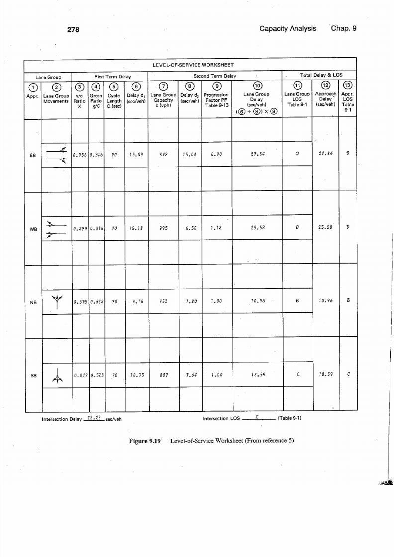
12. The planning application example shown in Figure 9.12 reveals that the intersection is
operating very close to capacity . Generate three minimum redesigns of the intersection in
order for the intersection to operate under capacity. Evaluate all three redesigns with theplanning method and recommend your preferred redesign. Hint: Study the four critical
movement sums.)
13. Assume the addition of one lane on each approach to the intersection shown in Figure
9.12. All added lanes will be for through traffic only. Evaluate this redesigned intersec
tion,using the planning method.
14. The resulting levels of service in.the operations application example are not very balanced
between the east-west and north-south streets (see Figure 9.19). Without changing the
cycle length, adjust the green phases shown in Figure 9.15 until the levels of service on the
two crossing streets are approximately the same. How much is the intersection delay of
22.22 seconds per vehicle reduced?
IS. How much would the intersection delay of 22.22 seconds per vehicle be reduced in Figure
9.19 if on all approaches the traffic arrived in dense platoons at (a) the beginning of the
green phase or (b) the beginning of the red phase? Hint: Refer to Table 9.13 of 1985
HCM for progression factors.)
16. Compare the operations method of analysis contained in the 1985 HCM with the most
recent Australian method of analysis for signalized intersections. Identify differences and
similarities.
9.9 SELE TED REFEREN ES
1. Bureau of Public Roads, Highway Capacity Manual, BPR, Washington D. C., 1950, 147
pages.
2. Highway Research Board, Highway Capacity Manual 1965, Special Report 87, HRB, Wash-
ington D. C., 1966, 411 pages. ·
3. A. D. May, Intersection Capacity 1974: An Overview, Transportation Research Board Spe
cial Report 153 TRB, Washington D. C., 1975, pages 50-59.
4. Transportation Research Board, Interim Materials o Highway Capacity, Circular 212, TRB,
Washington D. C., January 1980, 272 pages.
5. Transportation Research Board, Highway Capacity Manual, Special Report 204, TRB, Wash
ington D. C., 1985, 474 pages.
6. Stephen L. M. Hockaday and Adib K. Kanafani, Developments in Airport Capacity Analysis,
Transportation Research, Vol. 8 1974, pages 171-180.
7. Adib Kanafani, Operational Procedures to Increase Runway Capacity, Journal o Transporta-
tion Engineering, Vol. 109, No.3 May 1983, pages 414-424.
8. Robert Horonjeff, Planning and Design o Airports, 2nd Edition, McGraw-Hill Book Com
pany, New York, 1975,460 pages.
9. V. R. Vuchic, Urban Public Transportation: Systems and Technology, Prentice Hall, Inc.,
Englewood Cliffs, N. 1. 1981. i
10. R. Roess; W. McShane, E. Linzer, and L. Pignataro, Freeway Capacity Analyses Procequres,
ITE Journal, Vol. 50, No. 12 December 1980, pages 16-20.
III
1
1.1. :
ilI
II I
I
II
I II
),

7/18/2019 May Traffic Flow Fundamentals
http://slidepdf.com/reader/full/may-traffic-flow-fundamentals 291/472

7/18/2019 May Traffic Flow Fundamentals
http://slidepdf.com/reader/full/may-traffic-flow-fundamentals 292/472

7/18/2019 May Traffic Flow Fundamentals
http://slidepdf.com/reader/full/may-traffic-flow-fundamentals 293/472

7/18/2019 May Traffic Flow Fundamentals
http://slidepdf.com/reader/full/may-traffic-flow-fundamentals 294/472

7/18/2019 May Traffic Flow Fundamentals
http://slidepdf.com/reader/full/may-traffic-flow-fundamentals 295/472

7/18/2019 May Traffic Flow Fundamentals
http://slidepdf.com/reader/full/may-traffic-flow-fundamentals 296/472

7/18/2019 May Traffic Flow Fundamentals
http://slidepdf.com/reader/full/may-traffic-flow-fundamentals 297/472

7/18/2019 May Traffic Flow Fundamentals
http://slidepdf.com/reader/full/may-traffic-flow-fundamentals 298/472

7/18/2019 May Traffic Flow Fundamentals
http://slidepdf.com/reader/full/may-traffic-flow-fundamentals 299/472

7/18/2019 May Traffic Flow Fundamentals
http://slidepdf.com/reader/full/may-traffic-flow-fundamentals 300/472

7/18/2019 May Traffic Flow Fundamentals
http://slidepdf.com/reader/full/may-traffic-flow-fundamentals 301/472

7/18/2019 May Traffic Flow Fundamentals
http://slidepdf.com/reader/full/may-traffic-flow-fundamentals 302/472

7/18/2019 May Traffic Flow Fundamentals
http://slidepdf.com/reader/full/may-traffic-flow-fundamentals 303/472

7/18/2019 May Traffic Flow Fundamentals
http://slidepdf.com/reader/full/may-traffic-flow-fundamentals 304/472

7/18/2019 May Traffic Flow Fundamentals
http://slidepdf.com/reader/full/may-traffic-flow-fundamentals 305/472

7/18/2019 May Traffic Flow Fundamentals
http://slidepdf.com/reader/full/may-traffic-flow-fundamentals 306/472

7/18/2019 May Traffic Flow Fundamentals
http://slidepdf.com/reader/full/may-traffic-flow-fundamentals 307/472

7/18/2019 May Traffic Flow Fundamentals
http://slidepdf.com/reader/full/may-traffic-flow-fundamentals 308/472
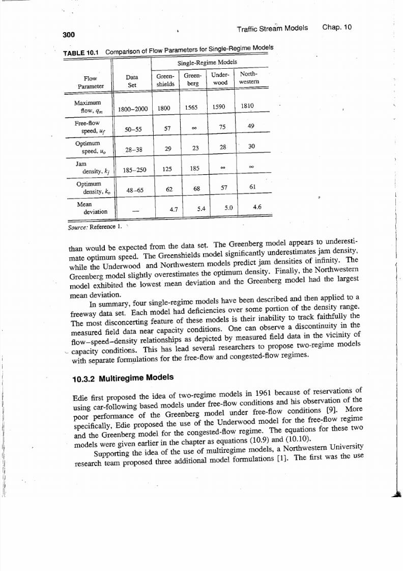
7/18/2019 May Traffic Flow Fundamentals
http://slidepdf.com/reader/full/may-traffic-flow-fundamentals 309/472

7/18/2019 May Traffic Flow Fundamentals
http://slidepdf.com/reader/full/may-traffic-flow-fundamentals 310/472
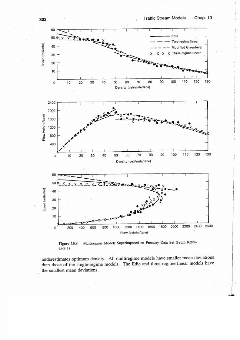
7/18/2019 May Traffic Flow Fundamentals
http://slidepdf.com/reader/full/may-traffic-flow-fundamentals 311/472

7/18/2019 May Traffic Flow Fundamentals
http://slidepdf.com/reader/full/may-traffic-flow-fundamentals 312/472

7/18/2019 May Traffic Flow Fundamentals
http://slidepdf.com/reader/full/may-traffic-flow-fundamentals 313/472

7/18/2019 May Traffic Flow Fundamentals
http://slidepdf.com/reader/full/may-traffic-flow-fundamentals 314/472

7/18/2019 May Traffic Flow Fundamentals
http://slidepdf.com/reader/full/may-traffic-flow-fundamentals 315/472

7/18/2019 May Traffic Flow Fundamentals
http://slidepdf.com/reader/full/may-traffic-flow-fundamentals 316/472

7/18/2019 May Traffic Flow Fundamentals
http://slidepdf.com/reader/full/may-traffic-flow-fundamentals 317/472

7/18/2019 May Traffic Flow Fundamentals
http://slidepdf.com/reader/full/may-traffic-flow-fundamentals 318/472

7/18/2019 May Traffic Flow Fundamentals
http://slidepdf.com/reader/full/may-traffic-flow-fundamentals 319/472

7/18/2019 May Traffic Flow Fundamentals
http://slidepdf.com/reader/full/may-traffic-flow-fundamentals 320/472

7/18/2019 May Traffic Flow Fundamentals
http://slidepdf.com/reader/full/may-traffic-flow-fundamentals 321/472

7/18/2019 May Traffic Flow Fundamentals
http://slidepdf.com/reader/full/may-traffic-flow-fundamentals 322/472

7/18/2019 May Traffic Flow Fundamentals
http://slidepdf.com/reader/full/may-traffic-flow-fundamentals 323/472

7/18/2019 May Traffic Flow Fundamentals
http://slidepdf.com/reader/full/may-traffic-flow-fundamentals 324/472

7/18/2019 May Traffic Flow Fundamentals
http://slidepdf.com/reader/full/may-traffic-flow-fundamentals 325/472

7/18/2019 May Traffic Flow Fundamentals
http://slidepdf.com/reader/full/may-traffic-flow-fundamentals 326/472

7/18/2019 May Traffic Flow Fundamentals
http://slidepdf.com/reader/full/may-traffic-flow-fundamentals 327/472

7/18/2019 May Traffic Flow Fundamentals
http://slidepdf.com/reader/full/may-traffic-flow-fundamentals 328/472

7/18/2019 May Traffic Flow Fundamentals
http://slidepdf.com/reader/full/may-traffic-flow-fundamentals 329/472

7/18/2019 May Traffic Flow Fundamentals
http://slidepdf.com/reader/full/may-traffic-flow-fundamentals 330/472
7 7
Shock ave Analysis
Flow-speed-density states change over space and time. When these changes of state
occur a boundary is established that demarks the time-space domain o one flow state
from another. This boundary is referred to s a shock wave. In some situations the
shock wave can be very mild, like a platoon of high-speed vehicles catching up to a
slightly slower moving vehicle. In other situations the shock wave can be a very
significant change in flow states, s when high-speed vehicles approach a queue of
stopped vehicles.
An introduction to shock waves was presented in Chapter 7, and the reader may
wish to review that material before proceeding further in this chapter. The introduction
w s limited to qualitative analysis, with primary attention given to flow discontinuities
or shock waves demarking boundaries between free-flow regimes and congested-flow
regimes. Two simple qualitative examples o shock waves were described: a signalized
intersection and a lane-drop location. The introduction concluded with further descrip
tion of shock waves and a classification of types of shock waves which included:
• Frontal stationary
• Backward forming*
• Forward recovery*
• Rear stationary
• Backward recovery*
• Forward forming*
In this chapter, attention will be directed toward quantitative analysis of all types
of shock waves. After a brief historical perspective, the chapter begins with the
*Using more general terminology, the phrase -moving can be substituted for -forming and
-recovery. _ /
32
I
•,I I

7/18/2019 May Traffic Flow Fundamentals
http://slidepdf.com/reader/full/may-traffic-flow-fundamentals 331/472
3 Shock Wave Analysis Chap.
derivation of shock wave equations. Then three examples are presented to illustrate the
application of shock wave theory. The first example is for a traffic signal location and
the second at t h ~ site where a slow-moving truck enters a highway. The last example is
of a pedestrian-way in a bottleneck situation. The text of the chapter concludes with a
discussion of shock wave analysis complexities and refinements. Selected problems andreferences are included at the end of the chapter.
11 1 AN HISTORICAL PERSPECTIVE
Richards [1] appears to have published the first paper on shock wave analysis applied to
transportation facilities. In his paper he assumed a linear speed-density relationship
and gave particular attention to the discontinuity of density. n the following year,
Lighthill and Whitham [2] published their renowned thesis on a theory of traffic flow on
long, crowded roads. t is still considered a monumental document and highly recommended.· It covers a wide selection of topics, including discussions on
flow-concentration curves, theory o bottlenecks, and flow at junctions. A research
group at Airborne Instruments Laboratory concerned with traffic congestion studied
backward waves [3].
In the late 1950s and early 1960s, several other researchers gave their attention to
shock wave analysis. These included Greenberg, Edie, and Foote [4 5] with their ~ o rin the New York tunnels; Franklin [6] with his proposed structure for .traffic shock
waves; and Pipes [7] with his fine summary paper reviewing previous w o r ~By the late 1960s several major textbooks were published. These included a
Transportation Research Board publication entitled n Introduction t Traffic Flow
Theory [8] which included the earlier Lighthill and Whitham [2] paper and the Pipes
paper [7]. Wohl and Martin, in their textbook Traffic System nalysis for Engineers
and Planners [9], discuss hydrodynamic analogies and their applications. n his text
book Traffic Flow Theory and Control [10], Drew reviewed the previous work on shock
waves, proposed an approach to bottleneck control, and finally i n t r o ~ u c e d the concepts
of momentum-kinetic energy and internal energy.
Pipes [11 12] continued his work with hydrodynamic theories describing wave
phenomenon. Rorbech [13], concerned with spill-backs from signalized intersections,
provided design procedures for the length o approach lanes. Gedough and Huber
prepared an excellent state-of-the-art chapter on hydrodynamic and kinematic traffic
models in their monograph on Traffic Flow Theory [14].
The most recent research publications have been concerned with the application of
shock wave analysis to signalized intersections and to highway facilities such as free
ways. Michalopoulos and associates [15 16] have reported on their research in apply- ·
ing shock wave analysis to signalized intersections, with particular concern with queue
dynamics and the effects of signal control. Leutzbach and Kohler, Wirasinghe, and
May have applied shock wave analysis to highways. Leutzbach and Kohler [17] have
used shock wave analysis to estimate delay due to incidents. Wirasinghe [18] has
applied shock wave analysis to estimate individual and total delays using graphical
j,.II
I
J
I· I

7/18/2019 May Traffic Flow Fundamentals
http://slidepdf.com/reader/full/may-traffic-flow-fundamentals 332/472
Sec. 11.2 Shock Wave Equations 3 3
means. May and associates [19, 20] have developed and continuously improved a free
way simulation model called FREQ, which includes the modeling of congestion
employing shock wave theory.
11 2 SHOCK WAVE EQUATIONS
Consider an uninterrupted segment of roadway for which a flow-density relationship is
known. Such a flow-density relationship is shown in Figure 11.1a. For some period of
time . a steady-state free-flow condition exists, as noted on the flow-density diagram as
state A. The flow density, and speed of state A are denoted as qA, kA, and uA, respec
tively. Then, for the following period of time, the input flow is less and a new steady
state free-flow condition exists, as noted on the flow-density diagram as state B. The
flow density, and speed of state B are denoted as qs, ks, and us, respectively. Note
that in state B, the speed us) will be higher, and these vehicles will catch up with vehi
cles in state over space and time.To visualize this more clearly, two additional sketches are included in Fig
ure 11.1. Figure 11.1 b is an illustration of the flow states in a distance-time diagram.
Note that the scales of distance and time are selected in such a manner that the rays
representing speeds in the d t diagram are parallel to the rays representing speeds in the
q k diagram. The heavy line identifies the shock wave or discontinuity between states
A and B, or stated in simple terms, it is the distance-time trace where the higher-speed
vehicles in flow state B join the lower-speed vehicles in flow state A. The symbol ro is
used to represent the shock wave and the subscripts A and B denote that the shock wave
lies between flow states A and B.
Figure 11.1 c shows a slice of the roadway at timet
which depicts the two flowstates. Three speeds with motion to the right are indicated: us, the vehicular speed in
flow state B; uA, the vehicular speed in the downstream flow state A; and roAs• the
shock wave speed between the two flow states. In this case, the direction of the shock
wave speed is fairly clear, but in more complicated situations,. where the direction may
not be clear, the analyst should assume the shock wave as a forward-moving shock
wave moving in the direction as traffic). That is, assume a positive shock wave speed.
If upon completing the analysis, the shock wave speed becomes negative, the shock
wave is a backward-moving shock wave and thus moving in the opposite direction as
traffic.
At the shock wave boundary, the number of vehicles leaving flow condition BNs) must be exactly equal to the number of vehicles entering flow condition NA)
since no vehicles are destroyed nor created. The speed of vehicles in flow condition B
just upstream of the shock wave boundary relative to the shock wave speed is
us roAB · The speed of vehicles in flow condition A, just downstream of the shock
wave boundary relative to the shock wave speed, is uA roAs). Therefore, Ns and NA
can be calculated using the following equations:
I
:

7/18/2019 May Traffic Flow Fundamentals
http://slidepdf.com/reader/full/may-traffic-flow-fundamentals 333/472
3 4
Density, k·
(a)
Time
(b)
Shock Wave Analysis Chap. 1 1
Figure 11.1 Shock Wave AnalysisJ (c) u n d a m ~ t a l s
NA =qAt= uA roA8 kAt
Setting N8 = NA and solving for roAB• equations 11.1) imd 11.2) become
(Us - (J)AB) kst = uA - (f)AB) kAt
and
qA qB J.q
f)AB = kA - ks = J.k
11.2)
11.3)
11.4)
Therefore, the shock wave speed between two states is equal to the change in flow
divided by the change in density. With flows expressed in vehicles per hour and densi
ties expressed in vehicles per mile, the shock wave speed is in units of miles per hour.
These units of measurement are confirmed by the sketches in Figure 11.1. It should
also be noted that since the shock wave speed is equal to the ratio of the change in flow
to the change in density, the s Iock wave can be depicted in the top sketch o Figure

7/18/2019 May Traffic Flow Fundamentals
http://slidepdf.com/reader/full/may-traffic-flow-fundamentals 334/472
Sec 11 3 Shock Waves at Signalized Intersections 3 5
11.1 as the slope of the line connecting flow conditions A and B. Since qA is larger
than q8 and kA is larger than k8 equation (11.4) results in a positive shock wave velo
city. This can also be seen in the sketches of Figure 11.1 since the slope of the line
representing the shock wave speed is up to the right, indicating a positive shock wave
speed J;IlOVing in the direction of traffic. Recall that a shock wave moving in the direc
tion of -traffic is called a forward-moving shock wave.
Now consider stationary and backward-moving shock waves in light of the
sketches of Figure 11.1. In these two examples, flow state B will remain unchanged,
while flow state A will be moved to the right side of the flow-density. curve marked C
and D. First consider flow condition C replacing flow condition A. In that situation, qc
is equal to q8 , and equation (11.4) indicates a shock w;:1ve speed of zero. This is
confirmed by Figure 1l.la since the line joining flow condition B with flow condition
C is a horizontal line. This is called a stationary shock wave.
Now consider flow condition D replacing flow condition A. In this situation q8 is
greater that qD, while k8 is less than kD and equation (11.4) indicates a negative shock
wave. This is confirmed by Figure 11.1a, since the line joining flow conditions B and
D is a downward sloping line. This is called a backward-moving shock wave.
The theory developed thus far assumes an instantaneous change in flow states and
implies that even when the roadway is free of traffic downstream, the drivers of lead
vehicles in a particular flow state will not increase their s p e e d s ~ These limitations and
possible.refinements are discussed in the last section of this chapter.
11 3 SHOCK WAVES AT SIGNALIZED INTERSECTIONS
Shock wave analysis. at signalized intersections is a common application becauseof
theconcern for the length of queues interfering with u p s t r ~ flow movements. Examples
include queues extending out of left-tum lanes into through traffic lanes and queues
extending upstream to block adjacent intersections.
Shock waves at signalized intersections can be analyzed if a flow-density rela
tionship is known for the approach to the signalized intersection and if the flow state of
the approaching t r f f i ~ is specifi.ed. For this example a flow-density curve and the
approaching traffic flow .state (A) are shown· in Figure 11.2a. A distance-time diagram
is shown in Figure 11.2b with d i s t ~ c e and time scales selected so that a given slope in·
the two diagrams represent a specific vehicle or shock wave speed. The stop line on
this approach to the signalized intersection is located at the traffic signal band, withgreen and red phases indicated as light and dark strips, fespectively
During time t 0 · to t 1, the signal is green and traffic proceeds on the approach,
through the intersection, and downstream under flow state A qA, uA, aild kA). The tra
jectory of individual vehicles are shown as dashed lines. At time t 1 the traffic signal
changes to red and the flow state immediately upstream of the stop line changes to state
B while the flow state immediately downstream changes to state D. Three shock waves
begin at time t 1 at the stop line: roAD, a forward-moving shock wave; roDs, a frontal
. stationary shock wave;· and r 8 a backward-moving shock wave . . The spee ds of these.
I
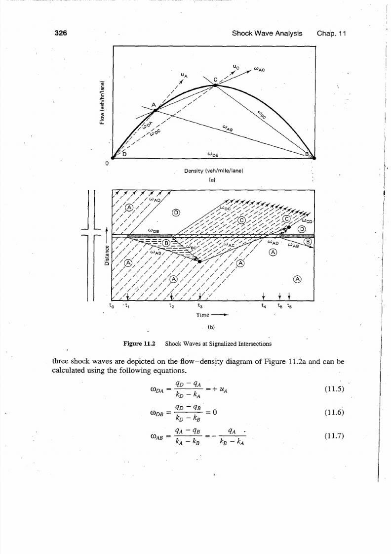
7/18/2019 May Traffic Flow Fundamentals
http://slidepdf.com/reader/full/may-traffic-flow-fundamentals 335/472
3 6 Shock Wave Analysis Chap. 1 1
0
Density veh/mile/lane)
a)
Jl
C
c
':i
®
to t , t2 t3 t4 t5 ts
ime
b)
Figure 11.2 Shock Waves at Signalized Intersections
three shock waves are depicted on the ftow-densi,ty diagram of Figure 11.2a and can be
calculated using the following equations.
qD qA11.5)ODA
kD kA=+ UA
qD qB=0 11.6)ODB =
kD ks
q qB qA11.7)OAB = =
k ks s kA

7/18/2019 May Traffic Flow Fundamentals
http://slidepdf.com/reader/full/may-traffic-flow-fundamentals 336/472
Sec. 11.3 Shock Waves at Signalized Intersections 3 7
These flow states of A B, and D continue until time t 2 when the signal changes to
green.· A new flow state is introduced flow state C) at time t 2 at the stop line when the
flow at the stop line increases from 0 to saturation flow. This causes two new shock
waves, roDe and ro8e while terminating shock wave roDE· The speeds of these two new
shock waves can be graphically seen in the flow-density diagram of Figure 1L2a and
calculated using the following equations:qD- qe
11.8)De =kD ke
=+ue
qB- qe qe11.9)ee = =
k8 - ke · k8 ke
. The flow states ofD, C B, and A continue until WAs and Wee intercept at time t 3•
The time interval between t 2 and t 3 can be calculated to be
t3
- t2
= r W B
lee - W B lJ-10)
where r is the effective duration of the red phase. The location of the queue dissipation
at time t 3 can also be calculated by means of the equation
r [ Wee) WAs)lM =
36Q0 Wee - W B 11.11)
·At time t3 a new forward-moving shock wave WAe is formed, and the two
backward-moving shock waves? WAs and Wee. are terminated.
The shock wave WAe is shown in Figure 11.2 and calculated using the equation
qA qeWAe =
k ke11.12)
The flow states of D, C, and A continue until time t5 ; but first consider time t4 • At
time t4 , the forward-moving shock wave WAe crosses the stop line, and the flow at the
stop line goes from a maximum flow .of qe to the arrival flow of CJA The period of time
from the start of the green phase until the stop-line discharge rate drops below its max
imum value t 2 to t4 ) can be c l c u l t ~ d to be
r WAs) Wee :
t4
- t 2 = + 1Wee - WAB WAe 11.13)
At t 5 , which is the beginning of the red phase, the shock wave pattern upstream
of the signal begins to repeat itself. However, the shock wave pattern downstream of
the signal deviates from the earlier pattern. Note that at the beginning of the red, shock
wave W D is formed, but it travels downstream only until it intercepts shock wave WAe·
At time t 6 , the WAe and wAD shock waves terminate, and a new shock wave, WeD, is
created. As long as the traffic demand and signal timing plan remain u n c h a n g ~ d the
shock wave pattern will repeat itself every signal cycle. I
7/18/2019 May Traffic Flow Fundamentals
http://slidepdf.com/reader/full/may-traffic-flow-fundamentals 337/472
3 8 Shock Wave Analysis Chap. 11
11 4 SHOCK WAVES ALONG A HIGHWAY
In their monograph entitled Traffic Flow Theory [14], Gerlough and Huber attributed
the following example to Edie. A steady flow state existed when a slow-moving truck
entered the roadway and proceeded to travel at a constant lower speed for some distance
before turning off the roadway. t is assumed that passing is not possible. The objectiveof the example problem is to construct a distance-time diagram on which all shock
waves are shown, as well as distance-time traces of selected vehicles.
A flow-density diagram and distance-time diagram are shown in Figure 11.3.
Prior to the truck turning onto the highway, the flow condition is represented by flow
state A. At time t 1 the truck enters the highway and travels at a :r:educed speed· Of ls,
causing the flow state behind t le truck to go to B and resulting in the flow state D
occurring in front of the truck. Two forward-moving shock waves and the truck trajec
tory begin at time t 1 at the location where the truck enters the highway: roAD roAB and
us rovs).
At time t2 the truck leaves the highway, and now with the unrestricted flow conditions ahead, the traffic can operate at capacity (flow state C). Two new shock waves
begin at time t2 at the location where the truck leaves the highway: rove and rose. The
shock wave, rove. is a forward-moving shock wave, while rose is a backward-moving
shock wave.
At time t3 the shock waves rose and roAs collide and terminate, which results in
another discontinuity between flow states C and A. This establishes a new forward
moving shock wave roeA.
The total picture of the trajectories of vehicles before, during, and after the truck
travel is shown in the lower portion of Figure 11.3. The result is the formation of five
forward-moving shock waves and one backward-movjng shock wave. The truck not
only affects the traffic stream when it is present on the roadway, but for sometime
thereafter. Imagine what the driver of the vehicle denoted as x experiences. When this
driver passes the point where the truck had entered, the truck had just exited from the
highway. The driver slows down and travels at the truck speed without knowing why. A
little later the driver speeds up some, but not as fast as his original speed. In summary,
this driver experiences congestion at a time period after the truck has exited and without
knowledge as to what caused the congestion.
Now consider some variations of this problem. Two situations will be considered.
In the first situation, all flow states will be assumed to remain the same except that flow
state A will vary from flow state to flow state C. f flow state A were assumed to be
near flow state D, the only significant change would be that shock wave ro B would
approach the speed of the truck us and the flow states B and C would be significantly
reduced. In other words, if the approach flow was extremely small, the truck would
have little influence on roadway operations.
Now consider the flow state A moving up the free-flow portion of the ·
flow-density curve until its flow is the same as the flow for flow state B qA =qs). The
shock wave ro B would become a stationary shock wave at the point where the truck
had entered the roadway. Flow states B and C would be larger than s ~ w n in Figure

7/18/2019 May Traffic Flow Fundamentals
http://slidepdf.com/reader/full/may-traffic-flow-fundamentals 338/472
Sec. 11.4 Shock Waves Along a Highway 3 9
Density veh/mile/lane)
tl j-
r ime
Figure 11.3 Shock Waves along a Highway
11.3. f the flow state A moved closer to the flow state C the shock wave roAB would
become a backward-moving shock wave, and the shock wave J)CA WOUld become a
.much slower forward-moving shock wave. The result would be a greatly increased
space-time domain with flow states B and C. The extreme case would be if the road
way were operating at capacity when the truck entered, the shock waves roAB and ro c
would be equal backward-moving shock waves and congested flow would never end.
Consider now the second situation. In this situation, all flow states will be
assumed to remain the same except that flow state B caused by the truck) will vary
over the complete range of the flow density diagram. f the truck enters the roadway at
a speed between free-flow speed and uA the truck will obviously not delay the other
vehicles in the traffic stream. In fact, the truck will be delayed by the other vehicles.)I

7/18/2019 May Traffic Flow Fundamentals
http://slidepdf.com/reader/full/may-traffic-flow-fundamentals 339/472
330 Shock Wave Analysis Chap.-11
If the truck enters the roadway at a speed between uA and uc the distance-time
diagram will be somewhat similar to Figure 11.3, except that WDs and WAs would be
steeper, and Wsc would be a slow-moving forward shock wave. The shock wave Wsc·
wouid not exist if the truck speed was uc.
Finally, consider that the truck enters the roadway at a speed close to zero. Theshock wave WAs would be a rather fast-moving backward shock wave, and the
space-time domain of flow states Band C would be significantly increased.
11.5 SHOCK WAVES ALONG A PEDESTRIAN WAY
The application of shock wave analysis is not limited to highway vehicular traffic.
Consider the discussion of pedestrian stream models in Chapter 10 and the following
example of shock wave analysis along a pedestrian-way.*
pedestrian-wayfor commuters connects two subway lines. Between, trains, the
flow in the pedestrian-way is almost nonexistent, while the flows increase almost tocapacity after a train arrival. Some subway reconstruction is planned, which will reduce
the capacity of the middle portion of the pedestrian-way. Given are the flow-density
diagram shown in Figure 11.4a, the demand flow flow state A after a train arrival, and
the reduced capacity qs) due to the subway reconstruction project. The objective of
the example problem is to construct a distance-time diagram on which all shock waves
are shown as well as selected distance-time projectories of pedestrians for that portion
of the pedestrian-way-upstream of the reconstruction area.
A subway train arrives and the first pedestrian r e c ~ e s the reconstruction area at
time t 1. The flow state just prior to t 1 is flow state D. The pedestrian arrival flow rate
becomes qA and immediately at t 1, the pedestrians begin to queue up going into thereconstruction area. Since the capacity of the reconstruction area is equivalent to qs,
the flow just upstream of the reconstruction area is limited to qs, resulting in flow state
B. The result is a flow discontinuity between flow states A and B, and a backward
moving shock wave WAs) is established. This shock wave continues until the last
passenger on the train reaches the upstream end of the congested area at time t 2 .
Thereafter, no further pedestrians arrive from this train and the last pedestrian proceeds
to the reconstructed area at speed us, and this also marks the discontinuity or shock
wave between flow states B and D. The last passenger from that subway train enters
the reconstruction area at t 3 . The queueing pattern repeats itself with the arrival of the
first passenger from the second train at time t 4 .
The analyst particularly would like to calculate the length of the maximum queue,
the time of occurrence of the maximum queue length, and the time when queueing
ceases. First consider the time of queueing t 3 - t 1 . If N persons leave the train and
use the pedestrian-way, and the capacity of the reconstruction area is equivalent to cis
the time of queue can be calculated as follows:
*The symbols that will be used for flow, s p e e ~ density, and shock wave speed are q, u k, and co
However, units for pedestrian flow characteristics are persons per minute per foot of width, feet per minute,
persons per square feet, and feet per minute, respectively. All flows must be for the total width of the
pedestrian-way.

7/18/2019 May Traffic Flow Fundamentals
http://slidepdf.com/reader/full/may-traffic-flow-fundamentals 340/472
·
Sec. 11.5
t
t
t
Shock Waves Along a Pedestrian-Way 33
:;::u§:
0
.;:
§';;;c0E
'.s;;:0
u::
'
a
D Density persons/ft2)
(a)
t2
i m e ~(b)
Figure 11.4 Shock aves along a Pedestrian-Way
N=qs t 3 - t i ) 11.14)
t3 - t (11.15)qB
Now consider the time of the occurrence of the maximum queue length Qm). Since
QmJ)AB = 11.16)
t2 - t
and

7/18/2019 May Traffic Flow Fundamentals
http://slidepdf.com/reader/full/may-traffic-flow-fundamentals 341/472

7/18/2019 May Traffic Flow Fundamentals
http://slidepdf.com/reader/full/may-traffic-flow-fundamentals 342/472
7/18/2019 May Traffic Flow Fundamentals
http://slidepdf.com/reader/full/may-traffic-flow-fundamentals 343/472
4 Shock Wave Analysis , Chap.
Similar observations can be drawn from Figures 11.3 and 11.4 of shock waves
along a highway and a pedestrian-way. The reader is encouraged to study these tw?
figures and to assess the effects of the various assumptions and limitations on the result
ing diagrams.
Limited literature is available to suggest possible refinements in shock wave
analysis. Lighthill and Whitham [2, 8] provide some insights as to how to handle
increased inflow situations, and shock wave analysis at bottlenecks and signalized inter
sections. Wohl and Martin [9] and a little later, Gerlough and Huber [14], reinforced the
Lighthill and Whitham approaches. Stephanopoulos et al. [16] provided further insights
into traffic queue dynamics at signalized intersections. The FREQ model [20]- has com
puterized shock wave ~ n l y s i s at freeway bottlenecks and has the capability of handling
interactive multiple bottlenecks, varying capacity over space and time, and varying
demand over space and time.
Shock wave analysis is an important tool in the analysis of flow and queueingproblems. Existing theory is available to approximate relatively simple problems.
Further research is needed to refine existing theory in order to more realistically
represent complex flow and queueing problems.
11 7 SELECTED PROBLEMS
1. Conduct a literature search on shock wave theory and application as applied to· transporta
tion for the period since 1980. Prepare a bibliography and classify into theory and applica
tions. Further, subclassify applications into highway vehicular and other, and under high
way vehicular subdivide into interrupted and uninterrupted flow situations. Comment on
the extensiveness (or lack thereof) of the literature.
2. Rework the example problem shown in Figure 1Ll by reversing the flow states A and B.
That is, have flow state B occur first, followed by flow state A. Draw diagrams like Figure
11.1 and derive equations (11.1) through (11.4).
3. Numerically solve the example problem shown in Figure 11.1 if flow states A and B are
defined as follows: uA and u8 are equal to 30 and 40 miles p.yr hour, respectively, and kand k are equal to 48 and 24 vehicles per mile per lane, respectively. How many vehicles
leave flow state B in a 1-hour period?
4. Use the flow-density diagram and combinations of the four flow states A, B, C, D of Fig
ure ll.la to draw distance-time diagrams (showing shock wave and vehicular trajectories)
that result in the following types of shock waves: (a) frontal stationary, (b) backward
forming, (c) forward recovery, (d) rear stationary, e) back ward recovery, and (f) forward
forming.
5. Repeat Problem 4 with numerical solutions. Assume that the flow-density diagram is .
based on a linear Greenshields model, u =5 0.417k, and the flows for states A, B, C,
and D are 1440, 960, 960, and 600 vehicles per hour per lane, respectively.
6. Numerically, solve the example problem shown in Figure 11.2 if the speed-density rela
tionship is linear and flow states A and C are defined as follows: uA and uc are equal to 40
·and 26 miles per hour, respectively, and kA and kc are equal to 24 and 60 vehicles per mile
per lane, respectively. Assume a 30-second green phase.

7/18/2019 May Traffic Flow Fundamentals
http://slidepdf.com/reader/full/may-traffic-flow-fundamentals 344/472
Chap Selected Problems 335
7. Plot a graph of the stopping shock wave wAs) in Figure 11.2 as a function of the arrival
flow qA)- Assume a linear speed-density relationship of u =5 0.417k.
8. Plot a graph of the starting shock wave wsc) in Figure 11.2 as a function of the discharge
flow qc). Assume a linear speed-density relationship u =5 0.417k.
9. Calculate the minimum length of the cycle that will not result in queue spillover to the next
signal cycle. Use the information provided in Problem 6.
10 Consider traffic flowing at 1000 vehicles per hour with a density of 20 vehicles per mile
and a speed of 50 miles per hour. A truck with a speed of 12 miles per hour enters the
traffic stream, travels for 2 miles, and then exits. No passing is possible and a dense flow
state results with a density of 100 vehicles per mile and a flow of 1200 vehicles per hour.
Draw the resulting distance-time diagram showing shock waves and vehicle projectories.
(Problem suggested by Edie.)
11 Using the information provided in Problem 10 and assuming a linear speed-density rela
tionship, draw the distance-time diagram (showing shock waves and vehicle projectories)
if the traffic was arriving at 1200 vehicles per hour.
12 By inspection of Figure 11.3, answer the following questions. (a) How fast would the
truck have to travel to eliminate shock waves? b) When would the shock wave wAB
become a rear stationary shock wave? (c) When would the shock wave wAs) become a
backward forming shock wave? and d) f traffic was arriving at capacity flow when
would shock waves wAs and Wsc intercept?
13. The individual lanes on a long, tangent, two-lane directional freeway have identical traffic
behavior patterns and each follows a linear speed-density relationship. It has been
observed that the capacity is 2000 vehicles per hour per lane and occurs at a speed of 25
miles per hour. On one particular day when the input flow rate was 1800 vehicles per hour
per lane, an accident occurred on the opposite side of the median which caused a gapers
block and caused the lane density to increase to 120 vehicles per mile. After 15 minutesthe accident was removed and traffic began to return to normal operations. Draw the
distance-time diagram showing shock waves and selected vehicle trajectories.
14 In Chapter 8 a directional freeway location was analyzed but queues were quantified in
terms of numbers of vehicles. Apply shock wave analysis techniques to determine the
length of queues at the end of each time period from 4:45 to 6:00 P.M.
15 n the problem graphically depicted in Figure 11.4, assume that the normal pedestrian-way
for commuters is 8 feet wide and the reduced pedestrian-way in the reconstruction area is 6
feet wide. A subway train arrives and discharges 540 passengers who proceed to the
pedestrian-way at a flow rate equivalent to a volume-capacity ratio of 0.9. Use appropri
ate pedestrian stream flow diagrams contained in Chapter 10. Plot resulting flow-densityand distance.:....time diagrams similar to Figure 11.4.
16 Using the information given in Problem 15 plot the minimum width of the pedestrian-way
in the reconstruction area that is needed as a function of the train headways. Assume no
queue overflows from one train s arrival until the next.
17 In evaluating the operational consequences of the reconstruction work, the operator is very
concerned that the queue due to the reconstruction does not extend upstream into the sub
way train platform area. Using the information given in Problem 15, plot the effe<;:t that
the width of the pedestrian-way in the reconstruction area has on the length of the ~ u e u eConsider only one train arrival.
7/18/2019 May Traffic Flow Fundamentals
http://slidepdf.com/reader/full/may-traffic-flow-fundamentals 345/472
336 Shock Wave Analysis Chap 11
18. Trains are expected to arrive at a specific station every 5 minutes. Four hundred and
twenty commuter passengers are predicted to be discharge<:\ onto the platform from every
train during the peak period.. From the platform, passengers are to be processed in a serial
fashion through five subsystems, which are oiscussed below.
1 From the platform to an escalator system, passengers will enter the first corridor which ·
is 100 feet long and 4 feet wide at capacity.
2. The escalator rises to the upper concourse level in 30 seconds over a horizon· distance
of 100 feet. The capacity of the escalator system is 70 passengers per minute.
3. The passengers then proceed along a second corridor identical to the dimensions of
the first corridor).
4 The passengers then pass through a turnstile system whose capacity is expected to be
50 passengers per minute.
5. The passengers then proceed along a third corridor identical to the dimensions of the
first corridor) into an open sidewalk area.
There are two tasks. The first task is to draw a distance-time diagram showing the trajectories of the first and last passenger off the first two trains and indicating the resulting
shock waves. The second task is to redesign the escalator and turnstile systems ·so that
there is no queueing backing into the escalator or train platform area.
19. In developing and applying shock wave analysis techniques a number of simplifying
assumptions were made. Identify these simplii):ing assumptions and discuss their implica
tions to the analysis portrayed in Figures 11.1, through 11.4. Refine the four figures quali
tatively to real-world conditions.
11 8 SELECTED REFERENCES
1. P. I. Richards, Shock Waves on the Highway, Operations Research Vol. 4, No.1, 1956,
pages 42-51.
2. M. H. Lighthill and G. B. Whitham, On Kinematic Waves: A Theory of Traffic Flow on
Long Crowded Roads, Proceedings of the Royal Society Series A Vol. 229, 1957, pages
317-345. Reprinted in Highway Research Board, Special Report 79, HRB, Washington,
D.C., 1964, pages 7-35).
3. Airborne Instruments Laboratory, Backward Waves in Highway Traffic Jams, Proceedings of
IRE Vol. 45, No. 1 1957, page 2A.
4. H. Greenberg, A Mathematical Analysis of Traffic Flow-Tunnel Traffic Capacity Study Portof New York Authority, New York, 1958.
5. H. Greenberg, An Analysis of Traffic Flow, Operations Research Vol. 7 No. 1 1959.
6. R. E. Franklin, The Structure of a Traffic Shock Wave, Civil Engineering Public Works
R eview Vol. 56 No. 662, 1961, pages 1186-1188.
7. L A Pipes, Hydrodynamic Approaches Part I: An Introduction to Traffic Flow Theory
Highway Research Board, Special Report 79, HRB, Washington, D.C., 1964, pages 3 5.
8. D. L Gerlough and D. G. Capelle, An Introduction to Traffic Flow Theory Highway
Research Board, Special Report 79 HRB, Washington, D.C., 1964, pages 3 35.
9. Martin Wohl and Brian V. Martin, Traffic System Analysis for Engineers and Planners
McGraw-Hill Book Company, New York, 1967, pages 338-345.

7/18/2019 May Traffic Flow Fundamentals
http://slidepdf.com/reader/full/may-traffic-flow-fundamentals 346/472

7/18/2019 May Traffic Flow Fundamentals
http://slidepdf.com/reader/full/may-traffic-flow-fundamentals 347/472

7/18/2019 May Traffic Flow Fundamentals
http://slidepdf.com/reader/full/may-traffic-flow-fundamentals 348/472

7/18/2019 May Traffic Flow Fundamentals
http://slidepdf.com/reader/full/may-traffic-flow-fundamentals 349/472

7/18/2019 May Traffic Flow Fundamentals
http://slidepdf.com/reader/full/may-traffic-flow-fundamentals 350/472

7/18/2019 May Traffic Flow Fundamentals
http://slidepdf.com/reader/full/may-traffic-flow-fundamentals 351/472

7/18/2019 May Traffic Flow Fundamentals
http://slidepdf.com/reader/full/may-traffic-flow-fundamentals 352/472

7/18/2019 May Traffic Flow Fundamentals
http://slidepdf.com/reader/full/may-traffic-flow-fundamentals 353/472

7/18/2019 May Traffic Flow Fundamentals
http://slidepdf.com/reader/full/may-traffic-flow-fundamentals 354/472

7/18/2019 May Traffic Flow Fundamentals
http://slidepdf.com/reader/full/may-traffic-flow-fundamentals 355/472

7/18/2019 May Traffic Flow Fundamentals
http://slidepdf.com/reader/full/may-traffic-flow-fundamentals 356/472

7/18/2019 May Traffic Flow Fundamentals
http://slidepdf.com/reader/full/may-traffic-flow-fundamentals 357/472
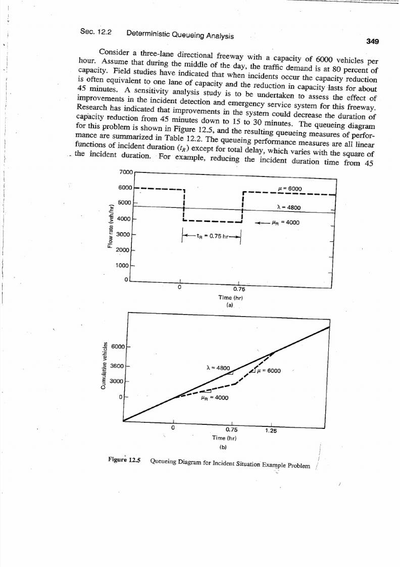
7/18/2019 May Traffic Flow Fundamentals
http://slidepdf.com/reader/full/may-traffic-flow-fundamentals 358/472

7/18/2019 May Traffic Flow Fundamentals
http://slidepdf.com/reader/full/may-traffic-flow-fundamentals 359/472

7/18/2019 May Traffic Flow Fundamentals
http://slidepdf.com/reader/full/may-traffic-flow-fundamentals 360/472

7/18/2019 May Traffic Flow Fundamentals
http://slidepdf.com/reader/full/may-traffic-flow-fundamentals 361/472

7/18/2019 May Traffic Flow Fundamentals
http://slidepdf.com/reader/full/may-traffic-flow-fundamentals 362/472

7/18/2019 May Traffic Flow Fundamentals
http://slidepdf.com/reader/full/may-traffic-flow-fundamentals 363/472

7/18/2019 May Traffic Flow Fundamentals
http://slidepdf.com/reader/full/may-traffic-flow-fundamentals 364/472

7/18/2019 May Traffic Flow Fundamentals
http://slidepdf.com/reader/full/may-traffic-flow-fundamentals 365/472

7/18/2019 May Traffic Flow Fundamentals
http://slidepdf.com/reader/full/may-traffic-flow-fundamentals 366/472

7/18/2019 May Traffic Flow Fundamentals
http://slidepdf.com/reader/full/may-traffic-flow-fundamentals 367/472

7/18/2019 May Traffic Flow Fundamentals
http://slidepdf.com/reader/full/may-traffic-flow-fundamentals 368/472

7/18/2019 May Traffic Flow Fundamentals
http://slidepdf.com/reader/full/may-traffic-flow-fundamentals 369/472
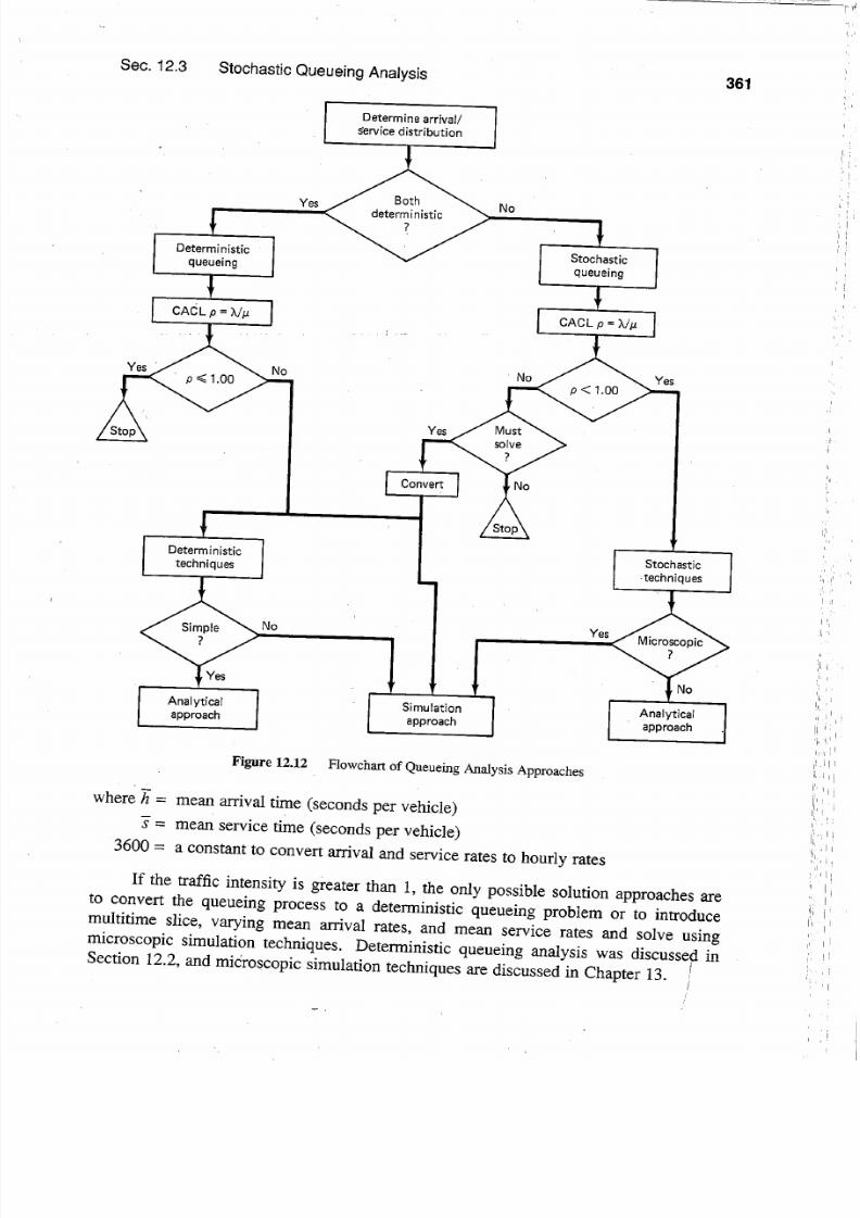
7/18/2019 May Traffic Flow Fundamentals
http://slidepdf.com/reader/full/may-traffic-flow-fundamentals 370/472

7/18/2019 May Traffic Flow Fundamentals
http://slidepdf.com/reader/full/may-traffic-flow-fundamentals 371/472
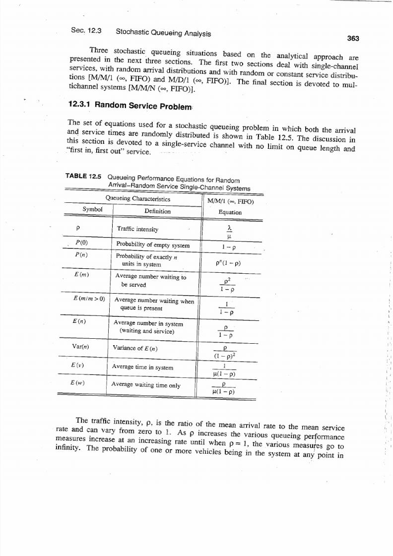
7/18/2019 May Traffic Flow Fundamentals
http://slidepdf.com/reader/full/may-traffic-flow-fundamentals 372/472
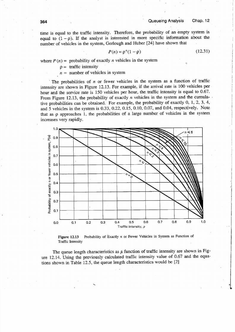
7/18/2019 May Traffic Flow Fundamentals
http://slidepdf.com/reader/full/may-traffic-flow-fundamentals 373/472

7/18/2019 May Traffic Flow Fundamentals
http://slidepdf.com/reader/full/may-traffic-flow-fundamentals 374/472

7/18/2019 May Traffic Flow Fundamentals
http://slidepdf.com/reader/full/may-traffic-flow-fundamentals 375/472

7/18/2019 May Traffic Flow Fundamentals
http://slidepdf.com/reader/full/may-traffic-flow-fundamentals 376/472

7/18/2019 May Traffic Flow Fundamentals
http://slidepdf.com/reader/full/may-traffic-flow-fundamentals 377/472

7/18/2019 May Traffic Flow Fundamentals
http://slidepdf.com/reader/full/may-traffic-flow-fundamentals 378/472

7/18/2019 May Traffic Flow Fundamentals
http://slidepdf.com/reader/full/may-traffic-flow-fundamentals 379/472

7/18/2019 May Traffic Flow Fundamentals
http://slidepdf.com/reader/full/may-traffic-flow-fundamentals 380/472

7/18/2019 May Traffic Flow Fundamentals
http://slidepdf.com/reader/full/may-traffic-flow-fundamentals 381/472

7/18/2019 May Traffic Flow Fundamentals
http://slidepdf.com/reader/full/may-traffic-flow-fundamentals 382/472

7/18/2019 May Traffic Flow Fundamentals
http://slidepdf.com/reader/full/may-traffic-flow-fundamentals 383/472

7/18/2019 May Traffic Flow Fundamentals
http://slidepdf.com/reader/full/may-traffic-flow-fundamentals 384/472

7/18/2019 May Traffic Flow Fundamentals
http://slidepdf.com/reader/full/may-traffic-flow-fundamentals 385/472

7/18/2019 May Traffic Flow Fundamentals
http://slidepdf.com/reader/full/may-traffic-flow-fundamentals 386/472

7/18/2019 May Traffic Flow Fundamentals
http://slidepdf.com/reader/full/may-traffic-flow-fundamentals 387/472

7/18/2019 May Traffic Flow Fundamentals
http://slidepdf.com/reader/full/may-traffic-flow-fundamentals 388/472

7/18/2019 May Traffic Flow Fundamentals
http://slidepdf.com/reader/full/may-traffic-flow-fundamentals 389/472

7/18/2019 May Traffic Flow Fundamentals
http://slidepdf.com/reader/full/may-traffic-flow-fundamentals 390/472

7/18/2019 May Traffic Flow Fundamentals
http://slidepdf.com/reader/full/may-traffic-flow-fundamentals 391/472

7/18/2019 May Traffic Flow Fundamentals
http://slidepdf.com/reader/full/may-traffic-flow-fundamentals 392/472

7/18/2019 May Traffic Flow Fundamentals
http://slidepdf.com/reader/full/may-traffic-flow-fundamentals 393/472
7/18/2019 May Traffic Flow Fundamentals
http://slidepdf.com/reader/full/may-traffic-flow-fundamentals 394/472

7/18/2019 May Traffic Flow Fundamentals
http://slidepdf.com/reader/full/may-traffic-flow-fundamentals 395/472

7/18/2019 May Traffic Flow Fundamentals
http://slidepdf.com/reader/full/may-traffic-flow-fundamentals 396/472

7/18/2019 May Traffic Flow Fundamentals
http://slidepdf.com/reader/full/may-traffic-flow-fundamentals 397/472

7/18/2019 May Traffic Flow Fundamentals
http://slidepdf.com/reader/full/may-traffic-flow-fundamentals 398/472
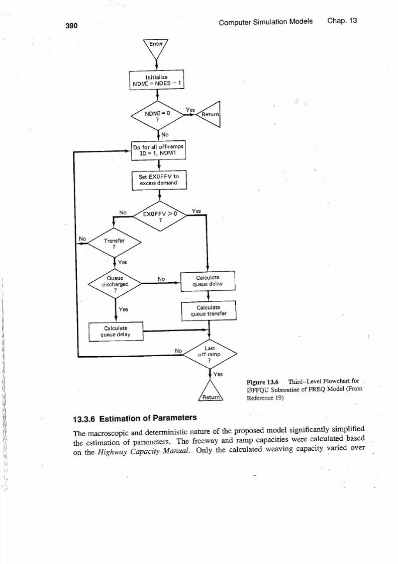
7/18/2019 May Traffic Flow Fundamentals
http://slidepdf.com/reader/full/may-traffic-flow-fundamentals 399/472

7/18/2019 May Traffic Flow Fundamentals
http://slidepdf.com/reader/full/may-traffic-flow-fundamentals 400/472

7/18/2019 May Traffic Flow Fundamentals
http://slidepdf.com/reader/full/may-traffic-flow-fundamentals 401/472

7/18/2019 May Traffic Flow Fundamentals
http://slidepdf.com/reader/full/may-traffic-flow-fundamentals 402/472

7/18/2019 May Traffic Flow Fundamentals
http://slidepdf.com/reader/full/may-traffic-flow-fundamentals 403/472

7/18/2019 May Traffic Flow Fundamentals
http://slidepdf.com/reader/full/may-traffic-flow-fundamentals 404/472

7/18/2019 May Traffic Flow Fundamentals
http://slidepdf.com/reader/full/may-traffic-flow-fundamentals 405/472

7/18/2019 May Traffic Flow Fundamentals
http://slidepdf.com/reader/full/may-traffic-flow-fundamentals 406/472

7/18/2019 May Traffic Flow Fundamentals
http://slidepdf.com/reader/full/may-traffic-flow-fundamentals 407/472

7/18/2019 May Traffic Flow Fundamentals
http://slidepdf.com/reader/full/may-traffic-flow-fundamentals 408/472

7/18/2019 May Traffic Flow Fundamentals
http://slidepdf.com/reader/full/may-traffic-flow-fundamentals 409/472

7/18/2019 May Traffic Flow Fundamentals
http://slidepdf.com/reader/full/may-traffic-flow-fundamentals 410/472

7/18/2019 May Traffic Flow Fundamentals
http://slidepdf.com/reader/full/may-traffic-flow-fundamentals 411/472

7/18/2019 May Traffic Flow Fundamentals
http://slidepdf.com/reader/full/may-traffic-flow-fundamentals 412/472

7/18/2019 May Traffic Flow Fundamentals
http://slidepdf.com/reader/full/may-traffic-flow-fundamentals 413/472

7/18/2019 May Traffic Flow Fundamentals
http://slidepdf.com/reader/full/may-traffic-flow-fundamentals 414/472

7/18/2019 May Traffic Flow Fundamentals
http://slidepdf.com/reader/full/may-traffic-flow-fundamentals 415/472

7/18/2019 May Traffic Flow Fundamentals
http://slidepdf.com/reader/full/may-traffic-flow-fundamentals 416/472
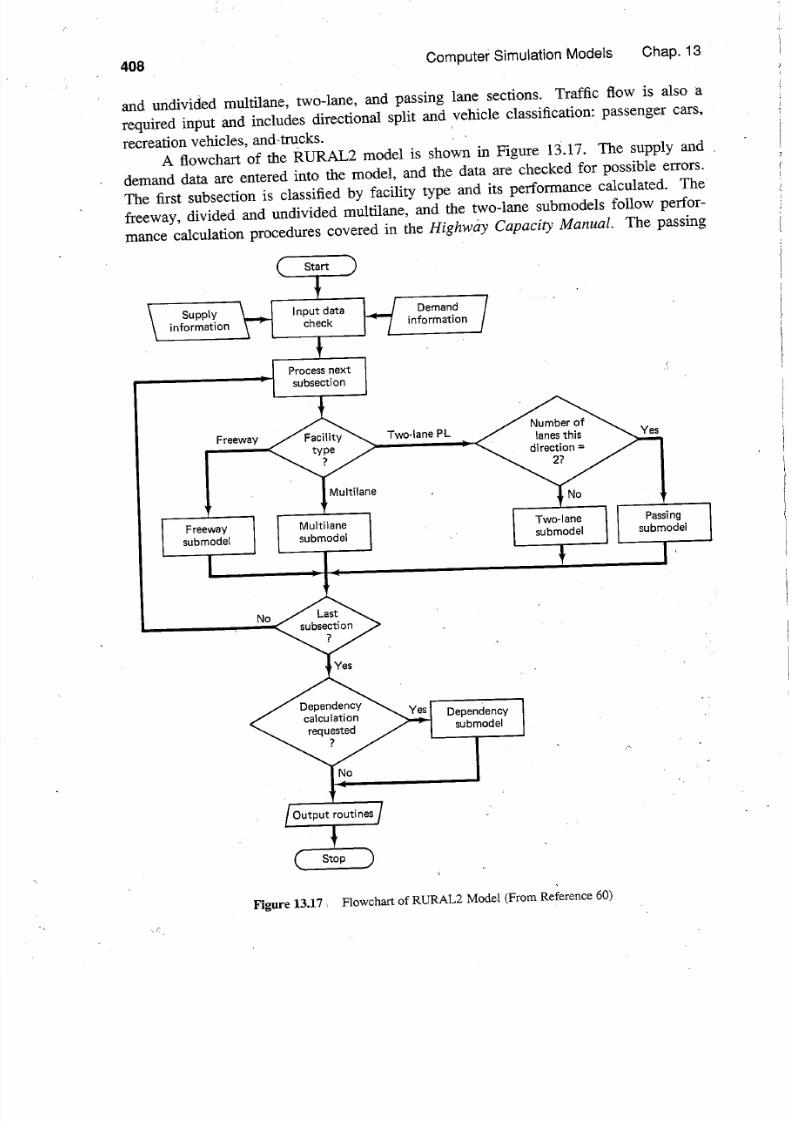
7/18/2019 May Traffic Flow Fundamentals
http://slidepdf.com/reader/full/may-traffic-flow-fundamentals 417/472

7/18/2019 May Traffic Flow Fundamentals
http://slidepdf.com/reader/full/may-traffic-flow-fundamentals 418/472

7/18/2019 May Traffic Flow Fundamentals
http://slidepdf.com/reader/full/may-traffic-flow-fundamentals 419/472

7/18/2019 May Traffic Flow Fundamentals
http://slidepdf.com/reader/full/may-traffic-flow-fundamentals 420/472

7/18/2019 May Traffic Flow Fundamentals
http://slidepdf.com/reader/full/may-traffic-flow-fundamentals 421/472

7/18/2019 May Traffic Flow Fundamentals
http://slidepdf.com/reader/full/may-traffic-flow-fundamentals 422/472

7/18/2019 May Traffic Flow Fundamentals
http://slidepdf.com/reader/full/may-traffic-flow-fundamentals 423/472
7/18/2019 May Traffic Flow Fundamentals
http://slidepdf.com/reader/full/may-traffic-flow-fundamentals 424/472

7/18/2019 May Traffic Flow Fundamentals
http://slidepdf.com/reader/full/may-traffic-flow-fundamentals 425/472

7/18/2019 May Traffic Flow Fundamentals
http://slidepdf.com/reader/full/may-traffic-flow-fundamentals 426/472

7/18/2019 May Traffic Flow Fundamentals
http://slidepdf.com/reader/full/may-traffic-flow-fundamentals 427/472

7/18/2019 May Traffic Flow Fundamentals
http://slidepdf.com/reader/full/may-traffic-flow-fundamentals 428/472

7/18/2019 May Traffic Flow Fundamentals
http://slidepdf.com/reader/full/may-traffic-flow-fundamentals 429/472
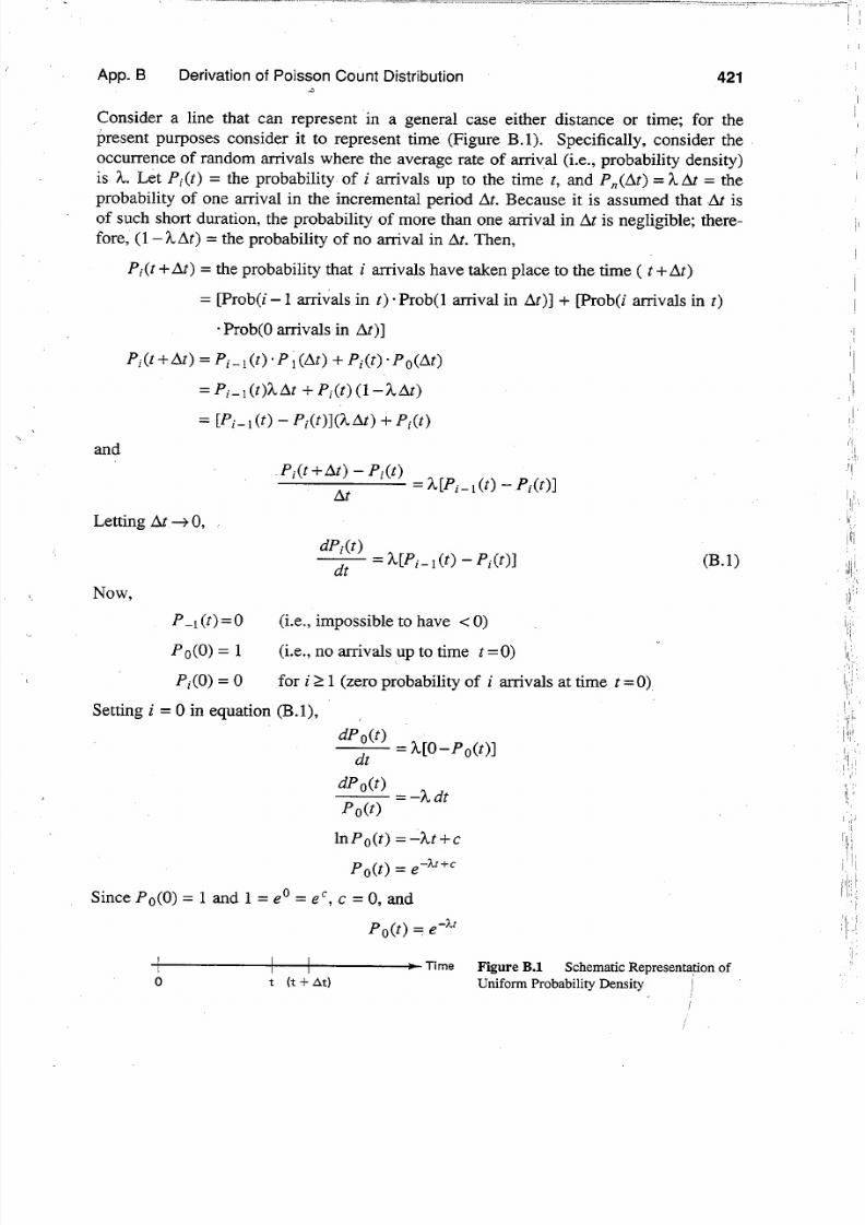
7/18/2019 May Traffic Flow Fundamentals
http://slidepdf.com/reader/full/may-traffic-flow-fundamentals 430/472

7/18/2019 May Traffic Flow Fundamentals
http://slidepdf.com/reader/full/may-traffic-flow-fundamentals 431/472
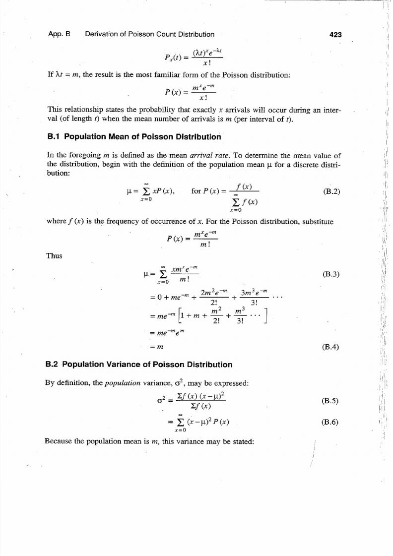
7/18/2019 May Traffic Flow Fundamentals
http://slidepdf.com/reader/full/may-traffic-flow-fundamentals 432/472

7/18/2019 May Traffic Flow Fundamentals
http://slidepdf.com/reader/full/may-traffic-flow-fundamentals 433/472

7/18/2019 May Traffic Flow Fundamentals
http://slidepdf.com/reader/full/may-traffic-flow-fundamentals 434/472

7/18/2019 May Traffic Flow Fundamentals
http://slidepdf.com/reader/full/may-traffic-flow-fundamentals 435/472

7/18/2019 May Traffic Flow Fundamentals
http://slidepdf.com/reader/full/may-traffic-flow-fundamentals 436/472

7/18/2019 May Traffic Flow Fundamentals
http://slidepdf.com/reader/full/may-traffic-flow-fundamentals 437/472
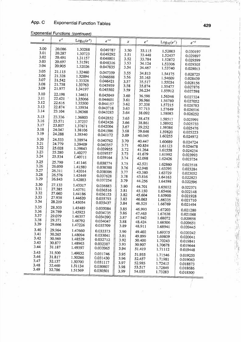
7/18/2019 May Traffic Flow Fundamentals
http://slidepdf.com/reader/full/may-traffic-flow-fundamentals 438/472

7/18/2019 May Traffic Flow Fundamentals
http://slidepdf.com/reader/full/may-traffic-flow-fundamentals 439/472

7/18/2019 May Traffic Flow Fundamentals
http://slidepdf.com/reader/full/may-traffic-flow-fundamentals 440/472

7/18/2019 May Traffic Flow Fundamentals
http://slidepdf.com/reader/full/may-traffic-flow-fundamentals 441/472

7/18/2019 May Traffic Flow Fundamentals
http://slidepdf.com/reader/full/may-traffic-flow-fundamentals 442/472

7/18/2019 May Traffic Flow Fundamentals
http://slidepdf.com/reader/full/may-traffic-flow-fundamentals 443/472

7/18/2019 May Traffic Flow Fundamentals
http://slidepdf.com/reader/full/may-traffic-flow-fundamentals 444/472

7/18/2019 May Traffic Flow Fundamentals
http://slidepdf.com/reader/full/may-traffic-flow-fundamentals 445/472

7/18/2019 May Traffic Flow Fundamentals
http://slidepdf.com/reader/full/may-traffic-flow-fundamentals 446/472

7/18/2019 May Traffic Flow Fundamentals
http://slidepdf.com/reader/full/may-traffic-flow-fundamentals 447/472

7/18/2019 May Traffic Flow Fundamentals
http://slidepdf.com/reader/full/may-traffic-flow-fundamentals 448/472

7/18/2019 May Traffic Flow Fundamentals
http://slidepdf.com/reader/full/may-traffic-flow-fundamentals 449/472

7/18/2019 May Traffic Flow Fundamentals
http://slidepdf.com/reader/full/may-traffic-flow-fundamentals 450/472

7/18/2019 May Traffic Flow Fundamentals
http://slidepdf.com/reader/full/may-traffic-flow-fundamentals 451/472

7/18/2019 May Traffic Flow Fundamentals
http://slidepdf.com/reader/full/may-traffic-flow-fundamentals 452/472

7/18/2019 May Traffic Flow Fundamentals
http://slidepdf.com/reader/full/may-traffic-flow-fundamentals 453/472

7/18/2019 May Traffic Flow Fundamentals
http://slidepdf.com/reader/full/may-traffic-flow-fundamentals 454/472

7/18/2019 May Traffic Flow Fundamentals
http://slidepdf.com/reader/full/may-traffic-flow-fundamentals 455/472

7/18/2019 May Traffic Flow Fundamentals
http://slidepdf.com/reader/full/may-traffic-flow-fundamentals 456/472

7/18/2019 May Traffic Flow Fundamentals
http://slidepdf.com/reader/full/may-traffic-flow-fundamentals 457/472

7/18/2019 May Traffic Flow Fundamentals
http://slidepdf.com/reader/full/may-traffic-flow-fundamentals 458/472

7/18/2019 May Traffic Flow Fundamentals
http://slidepdf.com/reader/full/may-traffic-flow-fundamentals 459/472

7/18/2019 May Traffic Flow Fundamentals
http://slidepdf.com/reader/full/may-traffic-flow-fundamentals 460/472

7/18/2019 May Traffic Flow Fundamentals
http://slidepdf.com/reader/full/may-traffic-flow-fundamentals 461/472
7/18/2019 May Traffic Flow Fundamentals
http://slidepdf.com/reader/full/may-traffic-flow-fundamentals 462/472
7/18/2019 May Traffic Flow Fundamentals
http://slidepdf.com/reader/full/may-traffic-flow-fundamentals 463/472

7/18/2019 May Traffic Flow Fundamentals
http://slidepdf.com/reader/full/may-traffic-flow-fundamentals 464/472

7/18/2019 May Traffic Flow Fundamentals
http://slidepdf.com/reader/full/may-traffic-flow-fundamentals 465/472

7/18/2019 May Traffic Flow Fundamentals
http://slidepdf.com/reader/full/may-traffic-flow-fundamentals 466/472

7/18/2019 May Traffic Flow Fundamentals
http://slidepdf.com/reader/full/may-traffic-flow-fundamentals 467/472

7/18/2019 May Traffic Flow Fundamentals
http://slidepdf.com/reader/full/may-traffic-flow-fundamentals 468/472

7/18/2019 May Traffic Flow Fundamentals
http://slidepdf.com/reader/full/may-traffic-flow-fundamentals 469/472

7/18/2019 May Traffic Flow Fundamentals
http://slidepdf.com/reader/full/may-traffic-flow-fundamentals 470/472

7/18/2019 May Traffic Flow Fundamentals
http://slidepdf.com/reader/full/may-traffic-flow-fundamentals 471/472

7/18/2019 May Traffic Flow Fundamentals
http://slidepdf.com/reader/full/may-traffic-flow-fundamentals 472/472