Maximum Likelihood Estimation

Eric Zivot

May 14, 2001This version: November 15, 2009

1 Maximum Likelihood Estimation

1.1 The Likelihood Function

Let X1, . . . , Xn be an iid sample with probability density function (pdf) f(xi; θ),where θ is a (k × 1) vector of parameters that characterize f(xi; θ). For example, ifXi˜N(μ, σ

2) then f(xi; θ) = (2πσ2)−1/2 exp(− 12σ2(xi − μ)2) and θ = (μ, σ2)0. The

joint density of the sample is, by independence, equal to the product of the marginaldensities

f(x1, . . . , xn; θ) = f(x1; θ) · · · f(xn; θ) =nYi=1

f(xi; θ).

The joint density is an n dimensional function of the data x1, . . . , xn given the para-meter vector θ. The joint density1 satisfies

f(x1, . . . , xn; θ) ≥ 0Z· · ·Z

f(x1, . . . , xn; θ)dx1 · · · dxn = 1.

The likelihood function is defined as the joint density treated as a functions of theparameters θ :

L(θ|x1, . . . , xn) = f(x1, . . . , xn; θ) =nYi=1

f(xi; θ).

Notice that the likelihood function is a k dimensional function of θ given the datax1, . . . , xn. It is important to keep in mind that the likelihood function, being afunction of θ and not the data, is not a proper pdf. It is always positive butZ

· · ·Z

L(θ|x1, . . . , xn)dθ1 · · · dθk 6= 1.

1If X1, . . . ,Xn are discrete random variables, then f(x1, . . . , xn; θ) = Pr(X1 = x1, . . . ,Xn = xn)for a fixed value of θ.

1

To simplify notation, let the vector x = (x1, . . . , xn) denote the observed sample.Then the joint pdf and likelihood function may be expressed as f(x; θ) and L(θ|x).

Example 1 Bernoulli Sampling

Let Xi˜ Bernoulli(θ). That is, Xi = 1 with probability θ and Xi = 0 with proba-bility 1− θ where 0 ≤ θ ≤ 1. The pdf for Xi is

f(xi; θ) = θxi(1− θ)1−xi , xi = 0, 1

Let X1, . . . , Xn be an iid sample with Xi˜ Bernoulli(θ). The joint density/likelihoodfunction is given by

f(x; θ) = L(θ|x) =nYi=1

θxi(1− θ)1−xi = θni=1 xi(1− θ)n−

ni=1 xi

For a given value of θ and observed sample x, f(x; θ) gives the probability of observingthe sample. For example, suppose n = 5 and x = (0, . . . , 0). Now some values of θare more likely to have generated this sample than others. In particular, it is morelikely that θ is close to zero than one. To see this, note that the likelihood functionfor this sample is

L(θ|(0, . . . , 0)) = (1− θ)5

This function is illustrated in figure xxx. The likelihood function has a clear maximumat θ = 0. That is, θ = 0 is the value of θ that makes the observed sample x = (0, . . . , 0)most likely (highest probability)Similarly, suppose x = (1, . . . , 1). Then the likelihood function is

L(θ|(1, . . . , 1)) = θ5

which is illustrated in figure xxx. Now the likelihood function has a maximum atθ = 1.

Example 2 Normal Sampling

Let X1, . . . , Xn be an iid sample with Xi˜N(μ, σ2). The pdf for Xi is

f(xi; θ) = (2πσ2)−1/2 exp

µ− 1

2σ2(xi − μ)2

¶, −∞ < μ <∞, σ2 > 0, −∞ < x <∞

so that θ = (μ, σ2)0. The likelihood function is given by

L(θ|x) =nYi=1

(2πσ2)−1/2 exp

µ− 1

2σ2(xi − μ)2

¶

= (2πσ2)−n/2 exp

Ã− 1

2σ2

nXi=1

(xi − μ)2

!

2

Figure xxx illustrates the normal likelihood for a representative sample of size n = 25.Notice that the likelihood has the same bell-shape of a bivariate normal densitySuppose σ2 = 1. Then

L(θ|x) = L(μ|x) = (2π)−n/2 expÃ−12

nXi=1

(xi − μ)2

!NownXi=1

(xi − μ)2 =nXi=1

(xi − x+ x− μ)2 =nXi=1

£(xi − x)2 + 2(xi − x)(x− μ) + (x− μ)2

¤=

nXi=1

(xi − x)2 + n(x− μ)2

so that

L(μ|x) = (2π)−n/2 expÃ−12

"nXi=1

(xi − x)2 + n(x− μ)2

#!Since both (xi− x)2 and (x− μ)2 are positive it is clear that L(μ|x) is maximized atμ = x. This is illustrated in figure xxx.

Example 3 Linear Regression Model with Normal Errors

Consider the linear regression

yi = x0i(1×k)

β(k×1)

+ εi, i = 1, . . . , n

εi|xi ˜ iid N(0, σ2)

The pdf of εi|xi is

f(εi|xi;σ2) = (2πσ2)−1/2 expµ− 1

2σ2ε2i

¶The Jacobian of the transformation for εi to yi is one so the pdf of yi|xi is normalwith mean x0iβ and variance σ

2 :

f(yi|xi; θ) = (2πσ2)−1/2 expµ− 1

2σ2(yi − x0iβ)

2

¶where θ = (β0, σ2)0. Given an iid sample of n observations, y and X, the joint densityof the sample is

f(y|X; θ) = (2πσ2)−n/2 exp

Ã− 1

2σ2

nXi=1

(yi − x0iβ)2

!

= (2πσ2)−n/2 exp

µ− 1

2σ2(y−Xβ)0(y−Xβ)

¶3

The log-likelihood function is then

lnL(θ|y,X) = −n2ln(2π)− n

2ln(σ2)− 1

2σ2(y−Xβ)0(y−Xβ)

Example 4 AR(1) model with Normal Errors

To be completed

1.2 The Maximum Likelihood Estimator

Suppose we have a random sample from the pdf f(xi; θ) and we are interested inestimating θ. The previous example motives an estimator as the value of θ thatmakes the observed sample most likely. Formally, the maximum likelihood estimator,denoted θmle, is the value of θ that maximizes L(θ|x). That is, θmle solves

maxθ

L(θ|x)

It is often quite difficult to directly maximize L(θ|x). It usually much easier tomaximize the log-likelihood function lnL(θ|x). Since ln(·) is a monotonic functionthe value of the θ that maximizes lnL(θ|x) will also maximize L(θ|x). Therefore, wemay also define θmle as the value of θ that solves

maxθlnL(θ|x)

With random sampling, the log-likelihood has the particularly simple form

lnL(θ|x) = lnÃ

nYi=1

f(xi; θ)

!=

nXi=1

ln f(xi; θ)

Since the MLE is defined as a maximization problem, we would like know theconditions under which we may determine the MLE using the techniques of calculus.A regular pdf f(x; θ) provides a sufficient set of such conditions. We say the f(x; θ)is regular if

1. The support of the random variables X,SX = {x : f(x; θ) > 0}, does notdepend on θ

2. f(x; θ) is at least three times differentiable with respect to θ

3. The true value of θ lies in a compact set Θ

4

If f(x; θ) is regular then we may find the MLE by differentiating lnL(θ|x) andsolving the first order conditions

∂ lnL(θmle|x)∂θ

= 0

Since θ is (k × 1) the first order conditions define k, potentially nonlinear, equationsin k unknown values:

∂ lnL(θmle|x)∂θ

=

⎛⎜⎜⎝∂ lnL(θmle|x)

∂θ1...

∂ lnL(θmle|x)∂θk

⎞⎟⎟⎠The vector of derivatives of the log-likelihood function is called the score vector

and is denoted

S(θ|x) = ∂ lnL(θ|x)∂θ

By definition, the MLE satisfies

S(θmle|x) = 0Under random sampling the score for the sample becomes the sum of the scores foreach observation xi :

S(θ|x) =nXi=1

∂ ln f(xi; θ)

∂θ=

nXi=1

S(θ|xi)

where S(θ|xi) = ∂ ln f(xi;θ)∂θ

is the score associated with xi.

Example 5 Bernoulli example continued

The log-likelihood function is

lnL(θ|X) = ln³θ

ni=1 xi(1− θ)n−

ni=1 xi

´=

nXi=1

xi ln(θ) +

Ãn−

nXi=1

xi

!ln(1− θ)

The score function for the Bernoulli log-likelihood is

S(θ|x) = ∂ lnL(θ|x)∂θ

=1

θ

nXi=1

xi −1

1− θ

Ãn−

nXi=1

xi

!The MLE satisfies S(θmle|x) = 0, which after a little algebra, produces the MLE

θmle =1

n

nXi=1

xi.

Hence, the sample average is the MLE for θ in the Bernoulli model.

5

Example 6 Normal example continued

Since the normal pdf is regular, we may determine the MLE for θ = (μ, σ2) bymaximizing the log-likelihood

lnL(θ|x) = −n2ln(2π)− n

2ln(σ2)− 1

2σ2

nXi=1

(xi − μ)2.

The sample score is a (2× 1) vector given by

S(θ|x) =Ã

∂ lnL(θ|x)∂μ

∂ lnL(θ|x)∂σ2

!where

∂ lnL(θ|x)∂μ

=1

σ2

nXi=1

(xi − μ)

∂ lnL(θ|x)∂σ2

= −n2(σ2)−1 +

1

2(σ2)−2

nXi=1

(xi − μ)2

Note that the score vector for an observation is

S(θ|xi) =Ã

∂ ln f(θ|xi)∂μ

∂ ln f(θ|xi)∂σ2

!=

µ(σ2)−1(xi − μ)

−12(σ2)−1 + 1

2(σ2)−2(xi − μ)2

¶so that S(θ|x) =

Pni=1 S(θ|xi).

Solving S(θmle|x) = 0 gives the normal equations

∂ lnL(θmle|x)∂μ

=1

σ2mle

nXi=1

(xi − μmle) = 0

∂ lnL(θmle|x)∂σ2

= −n2(σ2mle)

−1 +1

2(σ2mle)

−2nXi=1

(xi − μmle)2 = 0

Solving the first equation for μmle gives

μmle =1

n

nXi=1

xi = x

Hence, the sample average is the MLE for μ. Using μmle = x and solving the secondequation for σ2mle gives

σ2mle =1

n

nXi=1

(xi − x)2.

Notice that σ2mle is not equal to the sample variance.

6

Example 7 Linear regression example continued

The log-likelihood is

lnL(θ|y,X) = −n2ln(2π)− n

2ln(σ2)

− 1

2σ2(y −Xβ)0(y −Xβ)

The MLE of θ satisfies S(θmle|y,X) = 0 where S(θ|y,X) = ∂∂θlnL(θ|y,X) is the

score vector. Now

∂ lnL(θ|y,X)∂β

=1

2σ2∂

∂β[y0y − 2y0Xβ + β0X 0Xβ]

= −(σ2)−1[−X 0y +X 0Xβ]

∂ lnL(θ|y,X)∂σ2

= −n2(σ2)−1 +

1

2(σ2)−2(y −Xβ)0(y −Xβ)

Solving ∂ lnL(θ|y,X)∂β

= 0 for β gives

βmle = (X0X)−1X 0y = βOLS

Next, solving ∂ lnL(θ|y,X)∂σ2

= 0 for σ2 gives

σ2mle =1

n(y −Xbβmle)

0(y −Xbβmle)

6= σ2OLS =1

n− k(y −XbβOLS)0(y −XbβOLS)

1.3 Properties of the Score Function

The matrix of second derivatives of the log-likelihood is called the Hessian

H(θ|x) = ∂2 lnL(θ|x)∂θ∂θ0

=

⎛⎜⎜⎝∂2 lnL(θ|x)

∂θ21· · · ∂2 lnL(θ|x)

∂θ1∂θk...

. . ....

∂2 lnL(θ|x)∂θk∂θ1

· · · ∂2 lnL(θ|x)∂θ2k

⎞⎟⎟⎠The information matrix is defined as minus the expectation of the Hessian

I(θ|x) = −E[H(θ|x)]

If we have random sampling then

H(θ|x) =nXi=1

∂2 ln f(θ|xi)∂θ∂θ0

=nXi=1

H(θ|xi)

7

and

I(θ|x) = −nXi=1

E[H(θ|xi)] = −nE[H(θ|xi)] = nI(θ|xi)

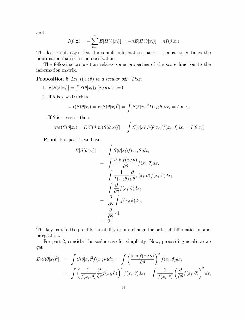
The last result says that the sample information matrix is equal to n times theinformation matrix for an observation.The following proposition relates some properties of the score function to the

information matrix.

Proposition 8 Let f(xi; θ) be a regular pdf. Then

1. E[S(θ|xi)] =RS(θ|xi)f(xi; θ)dxi = 0

2. If θ is a scalar then

var(S(θ|xi) = E[S(θ|xi)2] =Z

S(θ|xi)2f(xi; θ)dxi = I(θ|xi)

If θ is a vector then

var(S(θ|xi) = E[S(θ|xi)S(θ|xi)0] =Z

S(θ|xi)S(θ|xi)0f(xi; θ)dxi = I(θ|xi)

Proof. For part 1, we have

E[S(θ|xi)] =Z

S(θ|xi)f(xi; θ)dxi

=

Z∂ ln f(xi; θ)

∂θf(xi; θ)dxi

=

Z1

f(xi; θ)

∂

∂θf(xi; θ)f(xi; θ)dxi

=

Z∂

∂θf(xi; θ)dxi

=∂

∂θ

Zf(xi; θ)dxi

=∂

∂θ· 1

= 0.

The key part to the proof is the ability to interchange the order of differentiation andintegration.For part 2, consider the scalar case for simplicity. Now, proceeding as above we

get

E[S(θ|xi)2] =Z

S(θ|xi)2f(xi; θ)dxi =Z µ

∂ ln f(xi; θ)

∂θ

¶2f(xi; θ)dxi

=

Z µ1

f(xi; θ)

∂

∂θf(xi; θ)

¶2f(xi; θ)dxi =

Z1

f(xi; θ)

µ∂

∂θf(xi; θ)

¶2dxi

8

Next, recall that I(θ|xi) = −E[H(θ|xi)] and

−E[H(θ|xi)] = −Z

∂2 ln f(xi; θ)

∂θ2f(xi; θ)dxi

Now, by the chain rule

∂2

∂θ2ln f(xi; θ) =

∂

∂θ

µ1

f(xi; θ)

∂

∂θf(xi; θ)

¶= −f(xi; θ)−2

µ∂

∂θf(xi; θ)

¶2+ f(xi; θ)

−1 ∂2

∂θ2f(xi; θ)

Then

−E[H(θ|xi)] = −Z "−f(xi; θ)−2

µ∂

∂θf(xi; θ)

¶2+ f(xi; θ)

−1 ∂2

∂θ2f(xi; θ)

#f(xi; θ)dxi

=

Zf(xi; θ)

−1µ

∂

∂θf(xi; θ)

¶2dxi −

Z∂2

∂θ2f(xi; θ)dxi

= E[S(θ|xi)2]−∂2

∂θ2

Zf(xi; θ)dxi

= E[S(θ|xi)2].

1.4 Concentrating the Likelihood Function

In many situations, our interest may be only on a few elements of θ. Let θ = (θ1, θ2)and suppose θ1 is the parameter of interest and θ2 is a nuisance parameter (parameternot of interest). In this situation, it is often convenient to concentrate out the nuisanceparameter θ2 from the log-likelihood function leaving a concentrated log-likelihoodfunction that is only a function of the parameter of interest θ1.To illustrate, consider the example of iid sampling from a normal distribution.

Suppose the parameter of interest is μ and the nuisance parameter is σ2.We wish toconcentrate the log-likelihood with respect to σ2 leaving a concentrated log-likelihoodfunction for μ.We do this as follows. From the score function for σ2 we have the firstorder condition

∂ lnL(θ|x)∂σ2

= −n2(σ2)−1 +

1

2(σ2)−2

nXi=1

(xi − μ)2 = 0

Solving for σ2 as a function of μ gives

σ2(μ) =1

n

nXi=1

(xi − μ)2.

9

Notice that any value of σ2(μ) defined this way satisfies the first order condition∂ lnL(θ|x)

∂σ2= 0. If we substitute σ2(μ) for σ2 in the log-likelihood function for θ we get

the following concentrated log-likelihood function for μ :

lnLc(μ|x) = −n2ln(2π)− n

2ln(σ2(μ))− 1

2σ2(μ)

nXi=1

(xi − μ)2

= −n2ln(2π)− n

2ln

Ã1

n

nXi=1

(xi − μ)2

!

−12

Ã1

n

nXi=1

(xi − μ)2

!−1 nXi=1

(xi − μ)2

= −n2(ln(2π) + 1)− n

2ln

Ã1

n

nXi=1

(xi − μ)2

!Now we may determine the MLE for μ by maximizing the concentrated log-

likelihood function lnL2(μ|x). The first order conditions are

∂ lnLc(μmle|x)∂μ

=

Pni=1(xi − μmle)

1n

Pni=1(xi − μmle)

2= 0

which is satisfied by μmle = x provided not all of the xi values are identical.For some models it may not be possible to analytically concentrate the log-

likelihood with respect to a subset of parameters. Nonetheless, it is still possiblein principle to numerically concentrate the log-likelihood.

1.5 The Precision of the Maximum Likelihood Estimator

The likelihood, log-likelihood and score functions for a typical model are illustratedin figure xxx. The likelihood function is always positive (since it is the joint densityof the sample) but the log-likelihood function is typically negative (being the log ofa number less than 1). Here the log-likelihood is globally concave and has a uniquemaximum at θmle. Consequently, the score function is positive to the left of themaximum, crosses zero at the maximum and becomes negative to the right of themaximum.Intuitively, the precision of θmle depends on the curvature of the log-likelihood

function near θmle. If the log-likelihood is very curved or “steep” around θmle, thenθ will be precisely estimated. In this case, we say that we have a lot of informationabout θ. On the other hand, if the log-likelihood is not curved or “flat” near θmle,then θ will not be precisely estimated. Accordingly, we say that we do not have muchinformation about θ.The extreme case of a completely flat likelihood in θ is illustrated in figure xxx.

Here, the sample contains no information about the true value of θ because every

10

value of θ produces the same value of the likelihood function. When this happens wesay that θ is not identified. Formally, θ is identified if for all θ1 6= θ2 there exists asample x for which L(θ1|x) 6= L(θ2|x).The curvature of the log-likelihood is measured by its second derivative (Hessian)

H(θ|x) = ∂2 lnL(θ|x)∂θ∂θ0 . Since the Hessian is negative semi-definite, the information in

the sample about θ may be measured by −H(θ|x). If θ is a scalar then −H(θ|x) isa positive number. The expected amount of information in the sample about theparameter θ is the information matrix I(θ|x) = −E[H(θ|x)]. As we shall see, theinformation matrix is directly related to the precision of the MLE.

1.5.1 The Cramer-Rao Lower Bound

If we restrict ourselves to the class of unbiased estimators (linear and nonlinear)then we define the best estimator as the one with the smallest variance. With linearestimators, the Gauss-Markov theorem tells us that the ordinary least squares (OLS)estimator is best (BLUE). When we expand the class of estimators to include linearand nonlinear estimators it turns out that we can establish an absolute lower boundon the variance of any unbiased estimator θ of θ under certain conditions. Then if anunbiased estimator θ has a variance that is equal to the lower bound then we havefound the best unbiased estimator (BUE).

Theorem 9 Cramer-Rao Inequality

Let X1, . . . , Xn be an iid sample with pdf f(x; θ). Let θ be an unbiased estimatorof θ; i.e., E[θ] = θ. If f(x; θ) is regular then

var(θ) ≥ I(θ|x)−1

where I(θ|x) = −E[H(θ|x)] denotes the sample information matrix. Hence, theCramer-Rao Lower Bound (CRLB) is the inverse of the information matrix. If θ is avector then var(θ) ≥ I(θ|x)−1 means that var(θ)− I(θ|x) is positive semi-definite.

Example 10 Bernoulli model continued

To determine the CRLB the information matrix must be evaluated. The infor-mation matrix may be computed as

I(θ|x) = −E[H(θ|x)]

orI(θ|x) = var(S(θ|x))

11

Further, due to random sampling I(θ|x) = n · I(θ|xi) = n · var(S(θ|xi)). Now, usingthe chain rule it can be shown that

H(θ|xi) =d

dθS(θ|xi) =

d

dθ

µxi − θ

θ(1− θ)

¶= −

µ1 + S(θ|xi)− 2θS(θ|xi)

θ(1− θ)

¶The information for an observation is then

I(θ|xi) = −E[H(θ|xi)] =1 +E[S(θ|xi)]− 2θE[S(θ|xi)]

θ(1− θ)

=1

θ(1− θ)

since

E[S(θ|xi)] =E[xi]− θ

θ(1− θ)=

θ − θ

θ(1− θ)= 0

The information for an observation may also be computed as

I(θ|xi) = var(S(θ|xi) = varµ

xi − θ

θ(1− θ)

¶=

var(xi)

θ2(1− θ)2=

θ(1− θ)

θ2(1− θ)2

=1

θ(1− θ)

The information for the sample is then

I(θ|x) = n · I(θ|xi) =n

θ(1− θ)

and the CRLB is

CRLB = I(θ|x)−1 = θ(1− θ)

n

This the lower bound on the variance of any unbiased estimator of θ.Consider the MLE for θ, θmle = x. Now,

E[θmle] = E[x] = θ

var(θmle) = var(x) =θ(1− θ)

n

Notice that the MLE is unbiased and its variance is equal to the CRLB. Therefore,θmle is efficient.Remarks

12

• If θ = 0 or θ = 1 then I(θ|x) =∞ and var(θmle) = 0 (why?)

• I(θ|x) is smallest when θ = 12.

• As n → ∞, I(θ|x) → ∞ so that var(θmle) → 0 which suggests that θmle isconsistent for θ.

Example 11 Normal model continued

The Hessian for an observation is

H(θ|xi) =∂2 ln f(xi; θ)

∂θ∂θ0=

∂S(θ|xi)∂θ0

=

Ã∂2 ln f(xi;θ)

∂μ2∂2 ln f(xi;θ)

∂μ∂σ2

∂2 ln f(xi;θ)∂σ2∂μ

∂2 ln f(xi;θ)∂(σ2)2

!Now

∂2 ln f(xi; θ)

∂μ2= −(σ2)−1

∂2 ln f(xi; θ)

∂μ∂σ2= −(σ2)(xi − μ)

∂2 ln f(xi; θ)

∂σ2∂μ= −(σ2)(xi − μ)

∂2 ln f(xi; θ)

∂(σ2)2=

1

2(σ2)−2 − (σ2)−3(xi − μ)2

so that

I(θ|xi) = −E[H(θ|xi)]

=

µ(σ2)−1 E[(xi − μ)](σ2)−2

E[(xi − μ)](σ2)−2 12(σ2)−2 − (σ2)−3E[(xi − μ)2]

¶Using the results2

E[(xi − μ)] = 0

E

∙(xi − μ)2

σ2

¸= 1

we then have

I(θ|xi) =µ(σ2)−1 00 1

2(σ2)−2

¶The information matrix for the sample is then

I(θ|x) = n · I(θ|xi) =µ

n(σ2)−1 00 n

2(σ2)−2

¶2(xi − μ)2/σ2 is a chi-square random variable with one degree of freedom. The expected value

of a chi-square random variable is equal to its degrees of freedom.

13

and the CRLB is

CRLB = I(θ|x)−1 =µ

σ2

n0

0 2σ4

n

¶Notice that the information matrix and the CRLB are diagonal matrices. The CRLBfor an unbiased estimator of μ is σ2

nand the CRLB for an unbiased estimator of σ2

is 2σ4

n.

The MLEs for μ and σ2 are

μmle = x

σ2mle =1

n

nXi=1

(xi − μmle)2

Now

E[μmle] = μ

E[σ2mle] =n− 1n

σ2

so that μmle is unbiased whereas σ2mle is biased. This illustrates the fact that mles

are not necessarily unbiased. Furthermore,

var(μmle) =σ2

n= CRLB

and so μmle is efficient.The MLE for σ2 is biased and so the CRLB result does not apply. Consider the

unbiased estimator of σ2

s2 =1

n− 1

nXi=1

(xi − x)2

Is the variance of s2 equal to the CRLB? No. To see this, recall that

(n− 1)s2σ2

∼ χ2(n− 1)

Further, if X ∼ χ2(n− 1) then E[X] = n− 1 and var(X) = 2(n− 1). Therefore,

s2 =σ2

(n− 1)X

⇒ var(s2) =σ4

(n− 1)2var(X) =σ4

(n− 1)

Hence, var(s2) = σ4

(n−1) > CRLB = σ4

n.

Remarks

14

• The diagonal elements of I(θ|x)→∞ as n→∞

• I(θ|x) only depends on σ2

Example 12 Linear regression model continued

The score vector is given by

S(θ|y,X) =

µ−(σ2)−1[−X 0y +X 0Xβ]

−n2(σ2)−1 + 1

2(σ2)−2(y −Xβ)0(y −Xβ)

¶=

µ−(σ2)−1 (−X 0ε)

−n2(σ2)−1 + 1

2(σ2)−2ε0ε

¶where ε = y −Xβ. Now E[ε] = 0 and E[ε0ε] = nσ2 (since ε0ε/σ2 ∼ χ2(n)) so that

E[S(θ|y,X)] =µ

−(σ2)−1 (−X 0E[ε])−n2(σ2)−1 + 1

2(σ2)−2E[ε0ε]

¶=

µ00

¶To determine the Hessian and information matrix we need the second derivatives oflnL(θ|y,X) :

∂2 lnL(θ|y,X)∂β∂β0

=∂

∂β0¡−(σ2)−1[−X 0y +X 0Xβ]

¢= −(σ2)−1X 0X

∂2 lnL(θ|y,X)∂β∂σ2

=∂

∂σ2¡−(σ2)−1[−X 0y +X 0Xβ]

¢= −(σ2)−2X 0ε

∂2 lnL(θ|y,X)∂σ2∂β0

= −(σ2)−2ε0X

∂2 lnL(θ|y,X)∂ (σ2)2

=∂

∂σ2

µ−n2(σ2)−1 +

1

2(σ2)−2ε0ε

¶=

n

2(σ2)−2 − (σ2)−3ε0ε

Therefore,

H(θ|y,X) =µ−(σ2)−1X 0X −(σ2)−2X 0ε−(σ2)−2ε0X n

2(σ2)−2 − (σ2)−3ε0ε

¶and

I(θ|y,X) = −E[H(θ|y,X)]

=

µ−(σ2)−1X 0X −(σ2)−2X 0E[ε]−(σ2)−2E[ε]0X n

2(σ2)−2 − (σ2)−3E[ε0ε]

¶=

µ(σ2)−1X 0X 0

0 n2(σ2)−2

¶

15

Notice that the information matrix is block diagonal in β and σ2. The CRLB forunbiased estimators of θ is then

I(θ|y,X)−1 =µ

σ2(X 0X)−1 00 2

nσ4

¶Do theMLEs of β and σ2 achieve the CRLB? First, βmle is unbiased and var(βmle|X) =

σ2(X 0X)−1 = CRLB for an unbiased estimator for β. Hence, βmle is the most efficientunbiased estimator (BUE). This is an improvement over the Gauss-Markov theoremwhich says that βmle = βOLS is the most efficient linear and unbiased estimator(BLUE). Next, note that σ2mle is not unbiased (why) so the CRLB result does notapply. What about the unbiased estimator s2 = (n−k)−1(y−XβOLS)

0(y−XβOLS)?It can be shown that var(s2|X) = 2σ4

n−k > 2nσ4 = CRLB for an unbiased estimator of

σ2. Hence s2 is not the most efficient unbiased estimator of σ2.

1.6 Invariance Property of Maximum Likelihood Estimators

One of the attractive features of the method of maximum likelihood is its invarianceto one-to-one transformations of the parameters of the log-likelihood. That is, if θmle

is the MLE of θ and α = h(θ) is a one-to-one function of θ then αmle = h(θmle) is themle for α.

Example 13 Normal Model Continued

The log-likelihood is parameterized in terms of μ and σ2 and we have the MLEs

μmle = x

σ2mle =1

n

nXi=1

(xi − μmle)2

Suppose we are interested in the MLE for σ = h(σ2) = (σ2)1/2, which is a one-to-onefunction for σ2 > 0. The invariance property says that

σmle = (σ2mle)

1/2 =

Ã1

n

nXi=1

(xi − μmle)2

!1/2

1.7 Asymptotic Properties of Maximum Likelihood Estima-tors

Let X1, . . . , Xn be an iid sample with probability density function (pdf) f(xi; θ),where θ is a (k × 1) vector of parameters that characterize f(xi; θ). Under generalregularity conditions (see Hayashi Chapter 7), the ML estimator of θ has the followingasymptotic properties

16

1. θmlep→ θ

2.√n(θmle − θ)

d→ N(0, I(θ|xi)−1), where

I(θ|xi) = −E [H(θ|xi)] = −E∙∂ ln f(θ|xi)

∂θ∂θ0

¸That is,

avar(√n(θmle − θ)) = I(θ|xi)−1

Alternatively,

θmle ∼ N

µθ,1

nI(θ|xi)−1

¶= N(θ, I(θ|x)−1)

where I(θ|x) = nI(θ|xi) = information matrix for the sample.

3. θmle is efficient in the class of consistent and asymptotically normal estimators.That is,

avar(√n(θmle − θ))− avar(

√n(θ − θ)) ≤ 0

for any consistent and asymptotically normal estimator θ.

Remarks:

1. The consistency of the MLE requires the following

(a) Qn(θ) =1n

Pni=1 ln f(xi|θ)

p→ E[ln f(xi|θ)] = Q0(θ) uniformly in θ

(b) Q0(θ) is uniquely maximized at θ = θ0.

2. Asymptotic normality of θmle follows from an exact first order Taylor’s seriesexpansion of the first order conditions for a maximum of the log-likelihood aboutθ0:

0 = S(θmle|x) = S(θ0) +H(θ|x)(θmle − θ0), θ = λθmle + (1− λ)θ0

⇒ H(θ|x)(θmle − θ0) = −S(θ0)

⇒√n(θmle − θ0) = −

µ1

nH(θ|x)

¶−1√n

µ1

nS(θ0)

¶Now

H(θ|x) =1

n

nXi=1

H(θ|xi)p→ E[H(θ0|xi)] = −I(θ0|xi)

1√nS(θ0) =

1√n

nXi=1

S(θ0|xi) d→ N(0, I(θ0|xi))

17

Therefore√n(θmle − θ0)

d→ I(θ0|xi)−1N(0, I(θ0|xi))= N(0, I(θ0|xi)−1)

3. Since I(θ|xi) = −E[H(θ|xi)] = var(S(θ|xi)) is generally not known, avar(√n(θmle−

θ)) must be estimated. The most common estimates for I(θ|xi) are

I(θmle|xi) = −1n

nXi=1

H(θmle|xi)

I(θmle|xi) =1

n

nXi=1

S(θmle|xi)(θmle|xi)0

The first estimate requires second derivatives of the log-likelihood, whereasthe second estimate only requires first derivatives. Also, the second estimateis guaranteed to be positive semi-definite in finite samples. The estimate ofavar(

√n(θmle − θ)) then takes the form

davar(√n(θmle − θ)) = I(θmle|xi)−1

To prove consistency of the MLE, one must show that Q0(θ) = E[ln f(xi|θ)] isuniquely maximized at θ = θ0. To do this, let f(x, θ0) denote the true density andlet f(x, θ1) denote the density evaluated at any θ1 6= θ0. Define the Kullback-LeiblerInformation Criteria (KLIC) as

K(f(x, θ0), f(x, θ1)) = Eθ0

∙ln

f(x, θ0)

f(x, θ1)

¸=

Zln

f(x, θ0)

f(x, θ1)f(x, θ0)dx

where

lnf(x, θ0)

f(x, θ1)= ∞ if f(x, θ1) = 0 and f(x, θ0) > 0

K(f(x, θ0), f(x, θ1)) = 0 if f(x, θ0) = 0

The KLIC is a measure of the ability of the likelihood ratio to distinguish betweenf(x, θ0) and f(x, θ1) when f(x, θ0) is true. The Shannon-Komogorov InformationInequality gives the following result:

K(f(x, θ0), f(x, θ1)) ≥ 0

with equality if and only if f(x, θ0) = f(x, θ1) for all values of x.

Example 14 Asymptotic results for MLE of Bernoulli distribution parameters

18

Let X1, . . . , Xn be an iid sample with X ∼Bernoulli(θ). Recall,

θmle = X =1

n

nXi=1

Xi

I(θ|xi) =1

θ(1− θ)

The asymptotic properties of the MLE tell us that

θmlep→ θ

√n(θmle − θ)

d→ N (0, θ(1− θ))

Alternatively,

θmleA∼ N

µθ,θ(1− θ)

n

¶An estimate of the asymptotic variance of θmle is

avar(θmle) =θmle(1− θmle)

n=

x(1− x)

n

Example 15 Asymptotic results for MLE of linear regression model parameters

In the linear regression with normal errors

yi = x0iβ + εi, i = 1, . . . , n

εi|xi ˜ iid N(0, σ2)

the MLE for θ = (β0, σ2)0 isµβmle

σ2mle

¶=

µ(X 0X)−1X 0y

n−1(y −Xbβmle)0(y −Xbβmle)

¶and the information matrix for the sample is

I(θ|x) =µ

σ−2X 0X 00 n

2σ−4

¶The asymptotic results for MLE tell us thatµ

βmle

σ2mle

¶A∼ N

µµβσ2

¶,

µσ2(X 0X)−1 0

0 2nσ4

¶¶Further, the block diagonality of the information matrix implies that βmle is asymp-totically independent of σ2mle.

19

1.8 Relationship Between ML and GMM

Let X1, . . . , Xn be an iid sample from some underlying economic model. To do MLestimation, you need to know the pdf, f(xi|θ), of an observation in order to form thelog-likelihood function

lnL(θ|x) =nXi=1

ln f(xi|θ)

where θ ∈ Rp. The MLE satisfies the first order condtions

∂ lnL(θmle|x)∂θ

= S(θmle|x) = 0

For general models, the first order condtions are p nonlinear equations in p unknowns.Under regularity conditions, the MLE is consistent, asymptotically normally distrib-uted, and efficient in the class of asymptotically normal estimators:

θmle ∼ N

µθ,1

nI(θ|xi)−1

¶where I(θ|xi) = −E[H(θ|xi)] = E[S(θ|xi)S(θ|xi)0].To do GMM estimation, you need to know k ≥ p population moment condtions

E[g(xi, θ)] = 0

The GMM estimator matches sample moments with the population moments. Thesample moments are

gn(θ) =1

n

nXi=1

g(xi, θ)

If k > p, the efficient GMM estimator minimizes the objective function

J(θ, S−1) = ngn(θ)0S−1gn(θ)

where S = E[g(xi, θ)g(xi,θ)0]. The first order conditions are

∂J(θgmm, S−1)

∂θ= G0

n(θgmm)S−1gn(θgmm) = 0

Under regularity conditions, the efficient GMM estimator is consistent, asymptoti-cally normally distributed, and efficient in the class of asymptotically normal GMMestimators for a given set of moment conditions:

θgmm ∼ N

µθ,1

n(G0S−1G)−1

¶where G = E

h∂gn(θ)∂θ0

i.

20

The asymptotic efficiency of the MLE in the class of consistent and asymptoticallynormal estimators implies that

avar(θmle)− avar(θgmm) ≤ 0

That is, the efficient GMM estimator is generally less efficient than the ML estimator.The GMM estimator will be equivalent to the ML estimator if the moment condi-

tions happen to correspond with the score associated with the pdf of an observation.That is, if

g(xi, θ) = S(θ|xi)In this case, there are p moment conditions and the model is just identified. TheGMM estimator then satisfies the sample moment equations

gn(θgmm) = S(θgmm|x) = 0

which implies that θgmm = θmle. Since

G = E

∙∂S(θ|xi)

∂θ0

¸= E[H(θ|xi)] = −I(θ|xi)

S = E[S(θ|xi)S(θ|x0i)] = I(θ|xi)

the asymptotic variance of the GMM estimator becomes

(G0S−1G)−1 = I(θ|xi)−1

which is the asymptotic variance of the MLE.

1.9 Hypothesis Testing in a Likelihood Framework

Let X1, . . . , Xn be iid with pdf f(x, θ) and assume that θ is a scalar. The hypothesesto be tested are

H0 : θ = θ0 vs. H1 : θ 6= θ0

A statistical test is a decision rule based on the observed data to either reject H0 ornot reject H0.

1.9.1 Likelihood Ratio Statistic

Consider the likelihood ratio

λ =L(θ0|x)L(θmle|x)

=L(θ0|x)

maxθ L(θ|x)

which is the ratio of the likelihood evaluated under the null to the likelihood evaluatedat the MLE. By construction 0 < λ ≤ 1. If H0 : θ = θ0 is true, then we should see

21

λ ≈ 1; if H0 : θ = θ0 is not true then we should see λ < 1. The likelihood ratio(LR) statistic is a simple transformation of λ such that the value of LR is large ifH0 : θ = θ0 is true, and the value of LR is small when H0 : θ = θ0 is not true.Formally, the LR statistic is

LR = −2 lnλ = −2 ln L(θ0|x)L(θmle|x)

= −2[lnL(θ0|x)− lnL(θmle|x)]

From Figure xxx, notice that the distance between lnL(θmle|x) and lnL(θ0|x)depends on the curvature of lnL(θ|x) near θ = θmle. If the curvature is sharpe (i.e.,information is high) then LR will be large for θ0 values away from θmle. If, however,the curvature of lnL(θ|x) is flat (i.e., information is low) the LR will be small for θ0values away from θmle.Under general regularity conditions, if H0 : θ = θ0 is true then

LRd→ χ2(1)

In general, the degrees of freedom of the chi-square limiting distribution depends onthe number of restrictions imposed under the null hypothesis. The decision rule forthe LR statistic is to reject H0 : θ = θ0 at the α× 100% level if LR > χ21−α(1), whereχ21−α(1) is the (1−α)× 100% quantile of the chi-square distribution with 1 degree offreedom.

1.9.2 Wald Statistic

The Wald statistic is based directly on the asymptotic normal distribution of θmle :

θmle ∼ N(θ, I(θmle|x)−1)

where I(θmle|x) is a consistent estimate of the sample information matrix. An im-plication of the asymptotic normality result is that the usualy t-ratio for testingH0 : θ = θ0

t =θmle − θ0cSE(θmle)

=θmle − θ0qI(θmle|x)−1

=³θmle − θ0

´qI(θmle|x)

is asymptotically distributed as a standard normal random variable. Using the contin-uous mapping theorem, it follows that the square of the t-statistic is asymptoticallydistributed as a chi-square random variable with 1 degree of freedom. The Wald

22

statistic is defined to be simply the square of this t-ratio

Wald =

³θmle − θ0

´2I(θmle|x)−1

=³θmle − θ0

´2I(θmle|x)

Under general regularity conditions, if H0 : θ = θ0 is true, then

Waldd→ χ2(1)

The intuition behind the Wald statistic is illustrated in Figure xxx. If the curva-ture of lnL(θ|x) near θ = θmle is big (high information) then the squared distance³θmle − θ0

´2gets blown up when constructing the Wald statistic. If the curvature

of lnL(θ|x) near θ = θmle is low, then I(θmle|x) is small and the squared distance³θmle − θ0

´2gets attenuated when constucting the Wald statistic.

1.9.3 Lagrange Multiplier/Score Statistic

With ML estimation, θmle solves the first order conditions

0 =d lnL(θmle|x)

dθ= S(θmle|x)

If H0 : θ = θ0 is true, then we should expect that

0 ≈ d lnL(θ0|x)dθ

= S(θ0|x)

If H0 : θ = θ0 is not true, then we should expect that

0 6= d lnL(θ0|x)dθ

= S(θ0|x)

The Lagrange multiplier (score) statistic is based on how far S(θ0|x) is from zero.Recall the following properties of the score S(θ|xi). If H0 : θ = θ0 is true then

E[S(θ0|xi)] = 0

var(S(θ0|xi)) = I(θ0|xi)

Further, it can be shown that

√nS(θ0|x) =

1√n

nXi=1

S(θ0|xi) d→ N(0, I(θ0|xi))

23

so thatS(θ0|x) ∼ N(0, I(θ0|x))

This result motivates the statistic

LM =S(θ0|x)2I(θ0|x)

= S(θ0|x)2I(θ0|x)−1

Under general regularity conditions, if H0 : θ = θ0 is true, then

LMd→ χ2(1)

24