Generalized Method of Moments - UW Faculty Web …faculty.washington.edu/ezivot/econ583/gmm.pdf ·...

This is page iPrinter: Opaque this

1Generalized Method of Moments

1.1 Introduction

This chapter describes generalized method of moments (GMM) estima-tion for linear and non-linear models with applications in economics andfinance. GMM estimation was formalized by Hansen (1982), and since hasbecome one of the most widely used methods of estimation for modelsin economics and finance. Unlike maximum likelihood estimation (MLE),GMM does not require complete knowledge of the distribution of the data.Only specified moments derived from an underlying model are needed forGMM estimation. In some cases in which the distribution of the data isknown, MLE can be computationally very burdensome whereas GMM canbe computationally very easy. The log-normal stochastic volatility model isone example. In models for which there are more moment conditions thanmodel parameters, GMM estimation provides a straightforward way to testthe specification of the proposed model. This is an important feature thatis unique to GMM estimation.This chapter is organized as follows. GMM estimation for linear models

is described in Section 1.2. Section 1.3 describes methods for estimating theefficient weight matrix. Sections 1.4 and 1.5 give examples of estimation andinference using the S+Finmetrics function GMM. Section 1.6 describes GMMestimation and inference for nonlinear models. Section 1.7 provides numer-ous examples of GMM estimation of nonlinear models in finance includ-ing Euler equation asset pricing models, discrete-time stochastic volatilitymodels, and continous-time interest rate diffusion models.

ii 1. Generalized Method of Moments

The theory and notation for GMM presented herein follows the excel-lent treatment given in Hayashi (2000). Other good textbook treatments ofGMM at an intermediate level are given in Hamilton (1994), Ruud (2000),Davidson and MacKinnon (2004), and Greene (2004). The most compre-hensive textbook treatment of GMM is Hall (2005). Excellent surveys ofrecent developments in GMM are given in the special issues of the Journalof Business and Economic Statistics (1996, 2002). Discussions of GMMapplied to problems in finance are given in Ogaki (1992), Ferson (1995),Andersen and Sorensen (1996), Campbell, Lo and MacKinlay (1997), Jamesand Webber (2000), Cochrane (2001), Jagannathan and Skoulakis (2002),and Hall (2005).

1.2 Single Equation Linear GMM

Consider the linear regression model

yt = z0tδ0 + εt, t = 1, . . . , n (1.1)

where zt is an L × 1 vector of explanatory variables, δ0 is a vector ofunknown coefficients and εt is a random error term. The model (1.1) allowsfor the possibility that some or all of the elements of zt may be correlatedwith the error term εt, i.e., E[ztkεt] 6= 0 for some k. If E[ztkεi] 6= 0 thenztk is called an endogenous variable. It is well known that if zt containsendogenous variables then the least squares estimator of δ0 in (1.1) is biasedand inconsistent.Associated with the model (1.1), it is assumed that there exists a K × 1

vector of instrumental variables xt which may contain some or all of theelements of zt. Let wt represent the vector of unique and non-constantelements of {yt, zt,xt}. It is assumed that {wt} is a stationary and ergodicstochastic process.The instrumental variables xt satisfy the set of K orthogonality condi-

tions

E[gt(wt, δ0)] = E[xtεt] = E[xt(yt − z0tδ0)] = 0 (1.2)

where gt(wt, δ0) = xtεt = xt(yt−z0tδ0). Expanding (1.2), gives the relation

Σxy = Σxzδ0

where Σxy = E[xtyt] and Σxz = E[xtz0t]. For identification of δ0, it is

required that the K×L matrix E[xtz0t] = Σxz be of full rank L. This rank

condition ensures that δ0 is the unique solution to (1.2). Note, if K = L,then Σxz is invertible and δ0 may be determined using

δ0 = Σ−1xzΣxy

1.2 Single Equation Linear GMM iii

A necessary condition for the identification of δ0 is the order condition

K ≥ L (1.3)

which simply states that the number of instrumental variables must begreater than or equal to the number of explanatory variables in (1.1). IfK = L then δ0 is said to be (apparently) just identified; if K > L then δ0is said to be (apparently) over-identified; if K < L then δ0 is not identified.The word “apparently” in parentheses is used to remind the reader thatthe rank condition

rank(Σxz) = L (1.4)

must also be satisfied for identification.In the regression model (1.1), the error terms are allowed to be condi-

tionally heteroskedastic as well as serially correlated. For the case in whichεt is conditionally heteroskedastic, it is assumed that {gt} = {xtεt} is astationary and ergodic martingale difference sequence (MDS) satisfying

E[gtg0t] = E[xtx

0tε2t ] = S

where S is a non-singular K ×K matrix. The matrix S is the asymptoticvariance-covariance matrix of the sample moments g = n−1

Pnt=1 gt(wt, δ0).

This follows from the central limit theorem for ergodic stationary martin-gale difference sequences (see Hayashi page 106)

√ng =

1√n

nXt=1

xtεtd→ N(0,S)

where avar(g) = S denotes the variance-covariance matrix of the limitingdistribution of

√ng.

For the case in which εt is serially correlated and possibly conditionallyheteroskedastic as well, it is assumed that {gt} = {xtεt} is a stationaryand ergodic stochastic process that satisfies

√ng =

1√n

nXt=1

xtεtd→ N(0,S)

S =∞X

j=−∞Γj = Γ0 +

∞Xj=1

(Γj + Γ0j)

where Γj = E[gtg0t−j ] = E[xtx

0t−jεtεt−j ]. In the above, avar(g) = S is

also referred to as the long-run variance of g.

1.2.1 Definition of the GMM Estimator

The generalized method of moments (GMM) estimator of δ in (1.1) is con-structed by exploiting the orthogonality conditions (1.2). The idea is to cre-ate a set of estimating equations for δ by making sample moments match

iv 1. Generalized Method of Moments

the population moments defined by (1.2). The sample moments based on(1.2) for an arbitrary value δ are

gn(δ) =1

n

nXt=1

g(wt, δ) =1

n

nXt=1

xt(y − z0tδ)

=

1n

Pnt=1 x1t(y − z0tδ)

...1n

Pnt=1 xKt(y − z0tδ)

These moment conditions are a set of K linear equations in L unknowns.Equating these sample moments to the population moment E[xtεt] = 0gives the estimating equations

Sxy − Sxzδ = 0 (1.5)

where Sxy = n−1Pn

t=1 xtyt and Sxz = n−1Pn

t=1 xtz0t are the sample mo-

ments.If K = L (δ0 is just identified) and Sxz is invertible then the GMM

estimator of δ isδ = S−1xz Sxy

which is also known as the indirect least squares estimator. If K > Lthen there may not be a solution to the estimating equations (1.5). In thiscase, the idea is to try to find δ that makes Sxy − Sxzδ as close to zero aspossible. To do this, let W denote a K×K symmetric and positive definite

(p.d.) weight matrix, possibly dependent on the data, such that Wp→W

as n → ∞ with W symmetric and p.d. Then the GMM estimator of δ,denoted δ(W), is defined as

δ(W) = argminδ

J(δ,W)

where

J(δ,W) = ngn(δ)0Wgn(δ) (1.6)

= n(Sxy − Sxzδ)0W(Sxy − Sxzδ)Since J(δ,W) is a simple quadratic form in δ, straightforward calculusmay be used to determine the analytic solution for δ(W) :

δ(W) = (S0xzWSxz)−1S0xzWSxy (1.7)

Asymptotic Properties

Under standard regularity conditions (see Hayashi Chapter 3), it can beshown that

δ(W)p→ δ0

√n³δ(W)− δ0

´d→ N(0, avar(δ(W)))

1.2 Single Equation Linear GMM v

where

avar(δ(W)) = (Σ0xzWΣxz)−1Σ0xzWSWΣxz(Σ

0xzWΣxz)

−1 (1.8)

A consistent estimate of avar(δ(W)), denoted [avar(δ(W)), may be com-puted using

[avar(δ(W)) = (S0xzWSxz)−1S0xzWSWSxz(S

0xzWSxz)

−1 (1.9)

where S is a consistent estimate for S = avar(g).

The Efficient GMM Estimator

For a given set of instruments xt, the GMM estimator δ(W) is definefor an arbitrary positive definite and symmetric weight matrix W. Theasymptotic variance of δ(W) in (1.8) depends on the chosen weight matrixW. A natural question to ask is: What weight matrix W produces thesmallest value of avar(δ(W))? The GMM estimator constructed with thisweight matrix is called the efficient GMM estimator . Hansen (1982) showedthat efficient GMM estimator results from setting W = S−1 such thatS

p→ S. For this choice of W, the asymptotic variance formula (1.8) reducesto

avar(δ(S−1)) = (Σ0xzS−1Σxz)

−1 (1.10)

of which a consistent estimate is

[avar(δ(S−1)) = (S0xzS−1Sxz)−1 (1.11)

The efficient GMM estimator is defined as

δ(S−1) = argminδ

ngn(δ)0S−1gn(δ)

which requires a consistent estimate of S. However, consistent estimation ofS, in turn, requires a consistent estimate of δ. To see this, consider the casein which εt in (1.1) is conditionally heteroskedastic so that S = E[gtg

0t] =

E[xtx0tε2t ]. A consistent estimate of S has the form

1

S =1

n

nXt=1

xtx0tε2t =

1

n

nXt=1

xtx0t(yt − z0tδ)2

such that δp→ δ. Similar arguments hold for the case in which gt = xtεt is

a serially correlated and heteroskedastic process.

1Davidson and MacKinnon (1993, section 16.3) suggest using a simple degrees-of-freedom corrected estimate of S that replaces n−1 in (1.17) with (n− k) to improve thefinite sample performance of tests based on (1.11).

vi 1. Generalized Method of Moments

Two Step Efficient GMM

The two-step efficient GMM estimator utilizes the result that a consistentestimate of δ may be computed by GMM with an arbitrary positive definite

and symmetric weight matrix W such that Wp→ W. Let δ(W) denote

such an estimate. Common choices for W are W = Ik and W = S−1xx =(n−1X0X)−1, where X is an n× k matrix with tth row equal to x0t2. Then,a first step consistent estimate of S is given by

S(W) =1

n

nXt=1

xtx0t(yt − z0tδ(W))2 (1.12)

The two-step efficient GMM estimator is then defined as

δ(S−1(W)) = argminδ

ngn(δ)0S−1(W)gn(δ) (1.13)

Iterated Efficient GMM

The iterated efficient GMM estimator uses the two-step efficient GMMestimator δ(S−1(W)) to update the estimation of S in (1.12) and thenrecomputes the estimator in (1.13). The process is repeated (iterated) untilthe estimates of δ do not change significantly from one iteration to thenext. Typically, only a few iterations are required. The resulting estimator

is denoted δ(S−1iter). The iterated efficient GMM estimator has the same

asymptotic distribution as the two-step efficient estimator. However, infinite samples the two estimators may differ. As Hamilton (1994, page 413)points out, the iterated GMM estimator has the practical advantage overthe two-step estimator in that the resulting estimates are invariant withrespect to the scale of the data and to the initial weighting matrix W.

Continuous Updating Efficient GMM

This estimator simultaneously estimates S, as a function of δ, and δ. It isdefined as

δ(S−1CU ) = argminδ

ngn(δ)0S−1(δ)gn(δ) (1.14)

where the expression for S(δ) depends on the estimator used for S. Forexample, with conditionally heteroskedastic errors S(δ) takes the form

S(δ)=1

n

nXt=1

xtx0t(yt − z0tδ)2

2In the function GMM, the default initial weight matrix is the identity matrix.This can be changed by supplying a weight matrix using the optional argumentw=my.weight.matrix. Using W = S−1xx is often more numerically stable than usingW = Ik.

1.2 Single Equation Linear GMM vii

Hansen, Heaton and Yaron (1996) call δ(S−1CU ) the continuous updating(CU) efficient GMM estimator . This estimator is asymptotically equivalentto the two-step and iterated estimators, but may differ in finite samples.The CU efficient GMM estimator does not depend on an initial weight ma-trixW, and, like the iterated efficient GMM estimator, the numerical valueof CU estimator is invariant to the scale of the data. It is computationallymore burdensome than the iterated estimator, especially for large nonlin-ear models, and is more prone to numerical instability. However, Hansen,Heaton and Yaron find that the finite sample performance of the CU estima-tor, and test statistics based on it, is often superior to the other estimators.The good finite sample performance of the CU estimator relative to the it-erated GMM estimator may be explained by the connection between theCU estimator and empirical likelihood estimators. See Imbens (2002) andNewey and Smith (2004) for further discussion on the relationship betweenGMM estimators and empirical likelihood estimators.

The J-Statistic

The J-statistic, introduced in Hansen (1982), refers to the value of theGMM objective function evaluated using an efficient GMM estimator:

J = J(δ(S−1), S−1) = ngn(δ(S−1))0S−1gn(δ(S

−1)) (1.15)

where δ(S−1) denotes any efficient GMM estimator of δ and S is a consis-tent estimate of S. If K = L then J = 0, and if K > L then J > 0. Underregularity conditions (see Hayashi chapter 3) and if the moment conditions(1.2) are valid, then as n→∞

Jd→ χ2(K − L)

Hence, in a well specified overidentified model with valid moment conditionsthe J−statistic behaves like a chi-square random variable with degrees offreedom equal to the number of overidentifying restrictions. If the modelis mis-specified and or some of the moment conditions (1.2) do not hold(e.g., E[xitεt] = E[xit(yt − z0tδ0)] 6= 0 for some i) then the J−statistic willbe large relative to a chi-square random variable with K − L degrees offreedom.The J−statistic acts as an omnibus test statistic for model mis-specifica-

tion. A large J−statistic indicates a mis-specified model. Unfortunately, theJ−statistic does not, by itself, give any information about how the modelis mis-specified.

Normalized Moments

If the model is rejected by the J−statistic, it is of interested to know whythe model is rejected. To aid in the diagnosis of model failure, the magni-tudes of the individual elements of the normalized moments

√ngn(δ(S

−1))

viii 1. Generalized Method of Moments

may point the reason why the model is rejected by the J−statistic. Un-der the null hypothesis that the model is correct and the orthogonalityconditions are valid, the normalized moments satisfy

√ngn(δ(S

−1)) d→ N(0,S−Σxz[Σ0xzS−1Σxz]

−1Σ0xz)

As a result, for a well specified model the individual moment t−ratiosti = gn(δ(S

−1))i/SE(gn(δ(S−1))i), i = 1, . . . ,K (1.16)

where

SE(gn(δ(S−1))i =

³hS− Σxz[Σ

0xzS−1Σxz]

−1Σ0xzi/T´1/2ii

are asymptotically standard normal. When the model is rejected using theJ−statistic, a large value of ti indicates mis-specification with respect tothe ith moment condition. Since the rank of S−Σxz[Σ

0xzS−1Σxz]

−1Σ0xz isK − L, the interpretation of the moment t−ratios (1.16) may be difficultin models for which the degree of over-identification is small. In particular,if K − L = 1 then t1 = · · · = tK .

Two Stage Least Squares as Efficient GMM

If, in the linear GMM regression model (1.1), the errors are conditionallyhomoskedastic then

E[xtx0tε2t ] = σ2Σxx = S

A consistent estimate of S has the form S = σ2Sxx where σ2 p→ σ2. Typi-

cally,

σ2 = n−1nXt=1

(yt − z0tδ)2

where δ → δ0. The efficient GMM estimator becomes:

δ(σ−2S−1xx ) = (S0xzσ−2S−1xxSxz)

−1S0xzσ−2S−1xxSxy

= (S0xzS−1xxSxz)

−1S0xzS−1xxSxy

= δ(S−1xx )

which does not depend on σ2. The estimator δ(S−1xx ) is, in fact, identicalto the two stage least squares (TSLS) estimator of δ :

δ(S−1xx ) = (S0xzS−1xxSxz)

−1S0xzS−1xxSxy

= (Z0PXZ)−1Z0PXy

= δTSLS

where Z denotes the n×Lmatrix of observations with tth row z0t,X denotesthe n× k matrix of observations with tth row x0t, and PX = X(X

0X)−1X0

is the idempotent matrix that projects onto the columns of X.

1.3 Estimation of S ix

Using (1.10), the asymptotic variance of δ(S−1xx ) = δTSLS is

avar(δTSLS) = (Σ0xzS−1Σxz)

−1 = σ2(Σ0xzΣ−1xxΣxz)

−1

Although δ(S−1xx ) does not depend on σ2, a consistent estimate of theasymptotic variance does:

[avar(δTSLS) = σ2(S0xzS−1xxSxz)

−1

Similarly, the J-statistic also depends on σ2 and takes the form

J(δTSLS , σ−2S−1xx ) = n

(sxy − Sxz δTSLS)0S−1xx (sxy − Sxz δTSLS)σ2

The TSLS J-statistics is also known as Sargan’s statistic (see Sargan 1958).

1.3 Estimation of S

To compute any of the efficient GMM estimators, a consistent estimateof S = avar(g) is required. The method used to estimate S depends onthe time series properties of the population moment conditions gt. Twocases are generally considered. In the first case, gt is assumed to be seriallyuncorrelated but may be conditionally heteroskedastic. In the second case,gt is assumed to be serially correlated as well as potentially conditionallyheteroskedastic. The following sections discuss estimation of S in these twocases. Similar estimators were discussed in the context of linear regressionin Chapter 6, Section 5. In what follows, the assumption of a linear model(1.1) is dropped and the K moment conditions embodied in the vectorgt are assumed to be nonlinear functions of q ≤ K model parameters θand are denoted gt(θ). The moment conditions satisfy E[gt(θ0)] = 0 andS = avar(g) = avar(n−1

Pni=1 gt(θ0)).

1.3.1 Serially Uncorrelated Moments

In many situations the population moment conditions gt(θ0) form an ergodic-stationary MDS with an appropriate information set It. In this case,

S = avar(g) = E[gt(θ0)gt(θ0)0]

Following White (1982), a heteroskedasticity consistent (HC) estimate of Shas the form

SHC =1

n

nXt=1

gt(θ)gt(θ)0 (1.17)

x 1. Generalized Method of Moments

where θ is a consistent estimate of θ03. Davidson and MacKinnon (1993,

section 16.3) suggest using a simple degrees-of-freedom corrected estimateof S that replaces n−1 in (1.17) with (n−k)−1 to improve the finite sampleperformance of tests based on (1.11).

1.3.2 Serially Correlated Moments

If the population moment conditions gt(θ0) are an ergodic-stationary butserially correlated process then

S = avar(g) = Γ0 +∞Xj=1

(Γj + Γ0j)

where Γj = E[gt(θ0)gt−j(θ0)0]. In this case a heteroskedasticity and auto-correlation consistent (HAC) estimate of S has the form

SHAC =1

n

n−1Xj=1

wj,n(Γj(θ) + Γ0j(θ))

where wj,n (j = 1, . . . , bn) are kernel function weights, bn is a non-negative

bandwidth parameter that may depend on the sample size, Γj(θ)

= 1n

Pnt=j+1 gt(θ)gt−j(θ)

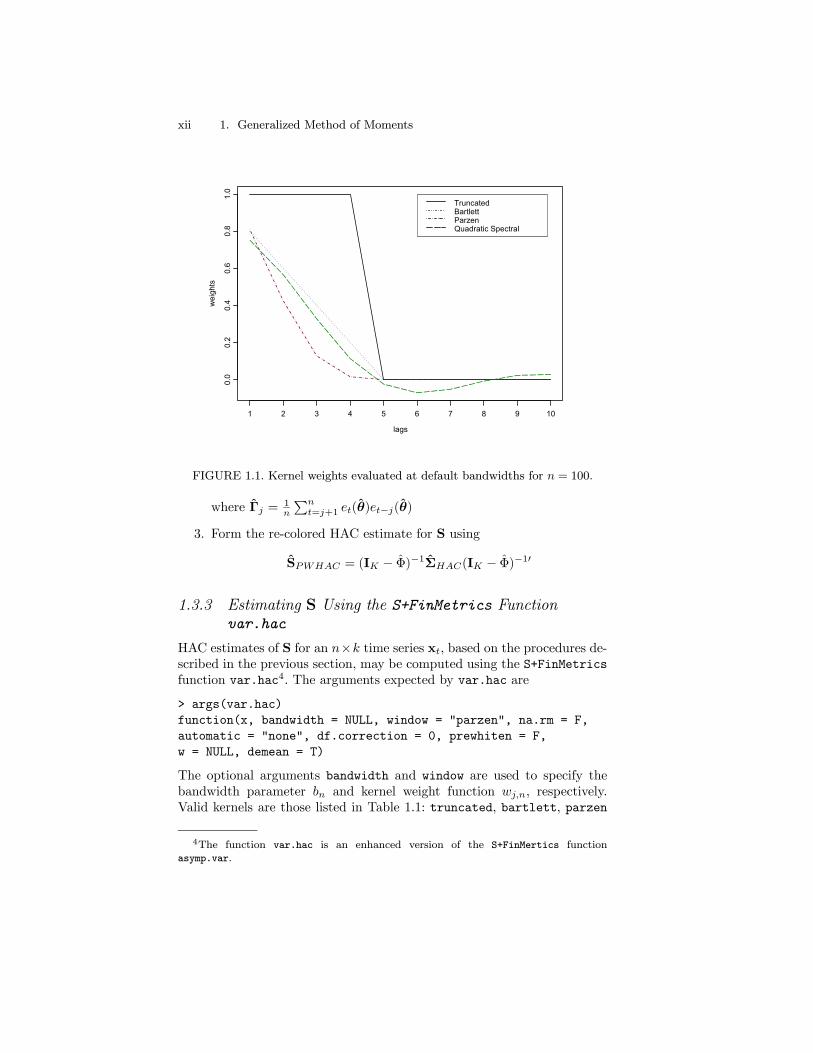
0, and θ is a consistent estimate of θ0. DifferentHAC estimates of S are distinguished by their kernel weights and band-width parameter. The most common kernel functions are listed in Table1.1. For all kernels except the quadratic spectral, the integer bandwidthparameter, bn, acts as a lag truncation parameter and determines howmany autocovariance matrices to include when forming SHAC . Figure 1.1illustrates the first ten kernel weights for the kernels listed in Table 1.1evaluated using the default values of bn for n = 100.The choice of kerneland bandwidth determine the statistical properties of SHAC . The truncatedkernel is often used if the moment conditions follow a finite order movingaverage process. However, the resulting estimate of S is not guaranteedto be positive definite. Use of the Bartlett, Parzen or quadratic spectralkernels ensures that SHAC will be positive semi-definite. For these kernels,Andrews (1991) studied the asymptotic properties SHAC . He showed thatSHAC is consistent for S provided that bn → ∞ as n → ∞. Furthermore,for each kernel, Andrews determined the rate at which bn →∞ to asymp-totically minimizeMSE(SHAC ,S). For the Bartlett, Parzen and quadraticspectral kernels the rates are n1/3, n1/5, and n1/5, respectively. Using theoptimal bandwidths, Andrews found that the SHAC based on the quadraticspectral kernel has the smallest asymptotic MSE, followed closely by SHAC

based on the Parzen kernel.

3For example, θ may be an inefficient GMM estimate based on an arbitrary p.d.weight matrix.

1.3 Estimation of S xi

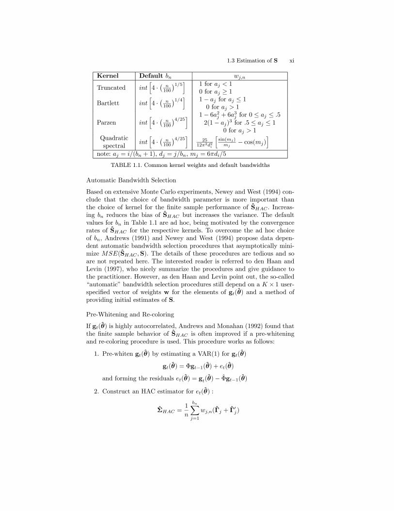
Kernel Default bn wj,n

Truncated inth4 · ¡ n

100

¢1/5i 1 for aj < 10 for aj ≥ 1

Bartlett inth4 · ¡ n

100

¢1/4i 1− aj for aj ≤ 10 for aj > 1

Parzen inth4 · ¡ n

100

¢4/25i 1− 6a2j + 6a3j for 0 ≤ aj ≤ .52(1− aj)

3 for .5 ≤ aj ≤ 10 for aj > 1

Quadraticspectral

inth4 · ¡ n

100

¢4/25i 2512π2d2i

hsin(mj)mj

− cos(mj)i

note: aj = i/(bn + 1), dj = j/bn, mj = 6πdi/5

TABLE 1.1. Common kernel weights and default bandwidths

Automatic Bandwidth Selection

Based on extensive Monte Carlo experiments, Newey and West (1994) con-clude that the choice of bandwidth parameter is more important thanthe choice of kernel for the finite sample performance of SHAC . Increas-ing bn reduces the bias of SHAC but increases the variance. The defaultvalues for bn in Table 1.1 are ad hoc, being motivated by the convergencerates of SHAC for the respective kernels. To overcome the ad hoc choiceof bn, Andrews (1991) and Newey and West (1994) propose data depen-dent automatic bandwidth selection procedures that asymptotically mini-mize MSE(SHAC ,S). The details of these procedures are tedious and soare not repeated here. The interested reader is referred to den Haan andLevin (1997), who nicely summarize the procedures and give guidance tothe practitioner. However, as den Haan and Levin point out, the so-called“automatic” bandwidth selection procedures still depend on a K × 1 user-specified vector of weights w for the elements of gt(θ) and a method ofproviding initial estimates of S.

Pre-Whitening and Re-coloring

If gt(θ) is highly autocorrelated, Andrews and Monahan (1992) found thatthe finite sample behavior of SHAC is often improved if a pre-whiteningand re-coloring procedure is used. This procedure works as follows:

1. Pre-whiten gt(θ) by estimating a VAR(1) for gt(θ)

gt(θ) = Φgt−1(θ) + et(θ)

and forming the residuals et(θ) = gt(θ)− Φgt−1(θ)2. Construct an HAC estimator for et(θ) :

ΣHAC =1

n

bnXj=1

wj,n(Γj + Γ0j)

xii 1. Generalized Method of Moments

lags

wei

ghts

1 2 3 4 5 6 7 8 9 10

0.0

0.2

0.4

0.6

0.8

1.0

TruncatedBartlettParzenQuadratic Spectral

FIGURE 1.1. Kernel weights evaluated at default bandwidths for n = 100.

where Γj =1n

Pnt=j+1 et(θ)et−j(θ)

3. Form the re-colored HAC estimate for S using

SPWHAC = (IK − Φ)−1ΣHAC(IK − Φ)−10

1.3.3 Estimating S Using the S+FinMetrics Functionvar.hac

HAC estimates of S for an n×k time series xt, based on the procedures de-scribed in the previous section, may be computed using the S+FinMetricsfunction var.hac4. The arguments expected by var.hac are

> args(var.hac)

function(x, bandwidth = NULL, window = "parzen", na.rm = F,

automatic = "none", df.correction = 0, prewhiten = F,

w = NULL, demean = T)

The optional arguments bandwidth and window are used to specify thebandwidth parameter bn and kernel weight function wj,n, respectively.Valid kernels are those listed in Table 1.1: truncated, bartlett, parzen

4The function var.hac is an enhanced version of the S+FinMertics functionasymp.var.

1.4 GMM Estimation Using the S+FinMetrics Function GMM xiii

and qs. If the bandwidth is not specified, then the default value for bn fromTable 1.1 is used for the specified kernel. The argument df.correctionspecifies a non-negative integer to be subtracted from the sample size toperform a degrees-of-freedom correction. The argument automatic deter-mines if the Andrews (1991) or Newey-West (1994) automatic bandwidthselection procedure is to be used to set bn. If automatic="andrews" orautomatic="nw" then the argument w must be supplied a vector of weightsfor each variable in x. The Andrews-Monahan (1992) VAR(1) pre-whiteningand re-coloring procedure is performed if prewhiten=T.

1.4 GMM Estimation Using the S+FinMetricsFunction GMM

GMM estimation of general linear and nonlinear models may be performedusing the S+FinMetrics function GMM. The arguments expected by GMM are

> args(GMM)

function(start, moments, control = NULL, scale = NULL, lower

= - Inf, upper = Inf, trace = T, method =

"iterative", w = NULL, max.steps = 100, w.tol = 0.0001,

ts = F, df.correction = T, var.hac.control =

var.hac.control(), w0.efficient = F, ...)

The required arguments are start, which is a vector of starting values forthe parameters of the model, and moments, which is an S-PLUS functionto compute the sample moment conditions used for estimating the model.The moments function must be of the form f(parm,...), where parm isa vector of L parameters, and return a matrix of dimension n×K givingthe GMM moment conditions x0tεt for t = 1, . . . , n. The optional argu-ments control, scale, lower and upper are used by the S-PLUS optimizerfunction nlregb. See the online help for nlregb and nlregb.control fordetails. Setting trace=T, displays iterative information from the optimiza-tion. The argument method determines the type of GMM estimation tobe performed. Valid choices are "iterative", for iterated GMM estima-tion, and "simultaneous", for continuous updating GMM estimation. Ifmethod="iterative" then the argument max.steps determines the num-ber of iterations to be performed. The argument w specifies the weight ma-trix used for constructing the GMM objective function (1.6)5. If w=NULL,then an estimate of the efficient weight matrix based on the asymptoticvariance of the sample moment conditions will be used. In this case, the ar-gument ts determines if an HC or HAC covariance estimator is computedand the arguments df.correction and var.hac.control control various

5The current version of GMM uses the inverse of w as the initial weight matrix.

xiv 1. Generalized Method of Moments

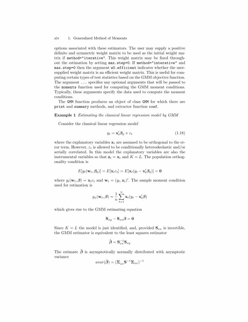
options associated with these estimators. The user may supply a positivedefinite and symmetric weight matrix to be used as the initial weight ma-trix if method="iterative". This weight matrix may be fixed through-out the estimation by setting max.step=0. If method="interative" andmax.step=0 then the argument w0.efficient indicates whether the user-supplied weight matrix is an efficient weight matrix. This is useful for com-puting certain types of test statistics based on the GMM objective function.The argument ... specifies any optional arguments that will be passed tothe moments function used for computing the GMM moment conditions.Typically, these arguments specify the data used to compute the momentconditions.The GMM function produces an object of class GMM for which there are

print and summary methods, and extractor function coef.

Example 1 Estimating the classical linear regression model by GMM

Consider the classical linear regression model

yt = x0tβ0 + εt (1.18)

where the explanatory variables xt are assumed to be orthogonal to the er-ror term. However, εt is allowed to be conditionally heteroskedastic and/orserially correlated. In this model the explanatory variables are also theinstrumental variables so that zt = xt and K = L. The population orthog-onality condition is

E[gt(wt,β0)] = E[xtεt] = E[xt(yt − x0tβ0)] = 0

where gt(wt,β) = xtεt and wt = (yt,xt)0. The sample moment condition

used for estimation is

gn(wt,β) =1

n

nXt=1

xt(yt − x0tβ)

which gives rise to the GMM estimating equation

Sxy − Sxxβ = 0

Since K = L the model is just identified, and, provided Sxx is invertible,the GMM estimator is equivalent to the least squares estimator

β = S−1xxSxy

The estimate β is asymptotically normally distributed with asymptoticvariance

avar(β) = (ΣxxS−1Σxx)

−1

1.4 GMM Estimation Using the S+FinMetrics Function GMM xv

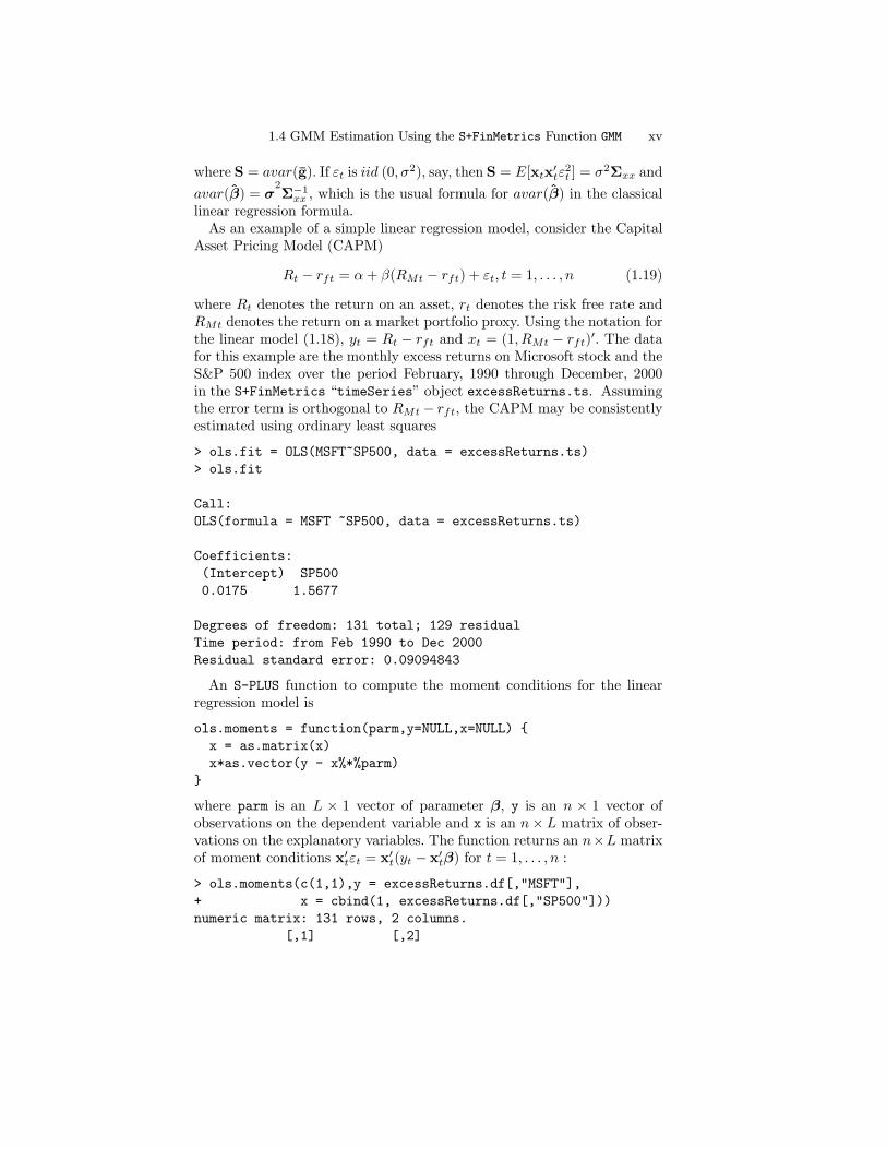
where S = avar(g). If εt is iid (0, σ2), say, then S = E[xtx

0tε2t ] = σ2Σxx and

avar(β) = σ2Σ−1xx , which is the usual formula for avar(β) in the classical

linear regression formula.As an example of a simple linear regression model, consider the Capital

Asset Pricing Model (CAPM)

Rt − rft = α+ β(RMt − rft) + εt, t = 1, . . . , n (1.19)

where Rt denotes the return on an asset, rt denotes the risk free rate andRMt denotes the return on a market portfolio proxy. Using the notation forthe linear model (1.18), yt = Rt − rft and xt = (1, RMt − rft)

0. The datafor this example are the monthly excess returns on Microsoft stock and theS&P 500 index over the period February, 1990 through December, 2000in the S+FinMetrics “timeSeries” object excessReturns.ts. Assumingthe error term is orthogonal to RMt − rft, the CAPM may be consistentlyestimated using ordinary least squares

> ols.fit = OLS(MSFT~SP500, data = excessReturns.ts)

> ols.fit

Call:

OLS(formula = MSFT ~SP500, data = excessReturns.ts)

Coefficients:

(Intercept) SP500

0.0175 1.5677

Degrees of freedom: 131 total; 129 residual

Time period: from Feb 1990 to Dec 2000

Residual standard error: 0.09094843

An S-PLUS function to compute the moment conditions for the linearregression model is

ols.moments = function(parm,y=NULL,x=NULL) {

x = as.matrix(x)

x*as.vector(y - x%*%parm)

}

where parm is an L × 1 vector of parameter β, y is an n × 1 vector ofobservations on the dependent variable and x is an n× L matrix of obser-vations on the explanatory variables. The function returns an n×L matrixof moment conditions x0tεt = x0t(yt − x0tβ) for t = 1, . . . , n :> ols.moments(c(1,1),y = excessReturns.df[,"MSFT"],

+ x = cbind(1, excessReturns.df[,"SP500"]))

numeric matrix: 131 rows, 2 columns.

[,1] [,2]

xvi 1. Generalized Method of Moments

[1,] -0.9409745 -0.0026713864

[2,] -0.9027093 -0.0161178959

...

[131,] -1.2480621 0.0009318206

To estimate the CAPM regression (1.19) with GMM assuming heteroskedas-tic errors use

> start.vals = c(0,1)

> names(start.vals) = c("alpha", "beta")

> gmm.fit = GMM(start.vals, ols.moments, max.steps = 1,

+ y = excessReturns.df[,"MSFT"],

+ x = cbind(1, excessReturns.df[,"SP500"]))

> class(gmm.fit)

[1] "GMM"

Notice how the data are passed to the function ols.moments through the... argument. The object gmm.fit returned by GMM is of class “GMM” andhas components

> names(gmm.fit)

[1] "parameters" "objective"

[3] "message" "grad.norm"

[5] "iterations" "r.evals"

[7] "j.evals" "scale"

[9] "normalized.moments" "vcov"

[11] "method" "df.J"

[13] "df.residual" "call"

The online help for GMM gives a complete description of these components6.Typing the name of the “GMM” object invokes the print method

> gmm.fit

Call:

GMM(start = start.vals, moments = ols.moments, max.steps = 1,

y = excessReturns.df[, "MSFT"], x = cbind(1,

excessReturns.df[, "SP500"]))

Coefficients:

alpha beta

0.0175 1.5677

6Since the linear model is just identified, the weight matrix in the GMM objectivefunction is irrelevant and so the weight.matrix component of gmm.fit is not returned.Also, the moments.vcov component is not returned since all of the normalized momentsare equal to zero.

1.4 GMM Estimation Using the S+FinMetrics Function GMM xvii

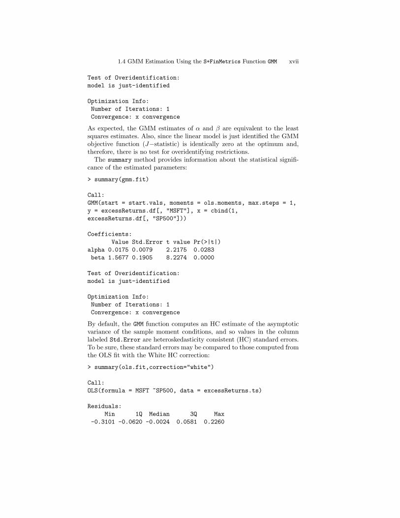
Test of Overidentification:

model is just-identified

Optimization Info:

Number of Iterations: 1

Convergence: x convergence

As expected, the GMM estimates of α and β are equivalent to the leastsquares estimates. Also, since the linear model is just identified the GMMobjective function (J−statistic) is identically zero at the optimum and,therefore, there is no test for overidentifying restrictions.The summary method provides information about the statistical signifi-

cance of the estimated parameters:

> summary(gmm.fit)

Call:

GMM(start = start.vals, moments = ols.moments, max.steps = 1,

y = excessReturns.df[, "MSFT"], x = cbind(1,

excessReturns.df[, "SP500"]))

Coefficients:

Value Std.Error t value Pr(>|t|)

alpha 0.0175 0.0079 2.2175 0.0283

beta 1.5677 0.1905 8.2274 0.0000



Optimization Info:


Convergence: x convergence

By default, the GMM function computes an HC estimate of the asymptoticvariance of the sample moment conditions, and so values in the columnlabeled Std.Error are heteroskedasticity consistent (HC) standard errors.To be sure, these standard errors may be compared to those computed fromthe OLS fit with the White HC correction:

> summary(ols.fit,correction="white")

Call:

OLS(formula = MSFT ~SP500, data = excessReturns.ts)

Residuals:

Min 1Q Median 3Q Max

-0.3101 -0.0620 -0.0024 0.0581 0.2260

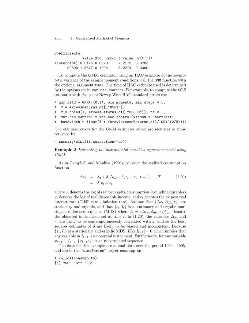
xviii 1. Generalized Method of Moments

Coefficients:

Value Std. Error t value Pr(>|t|)

(Intercept) 0.0175 0.0079 2.2175 0.0283

SP500 1.5677 0.1905 8.2274 0.0000

To compute the GMM estimator using an HAC estimate of the asymp-totic variance of the sample moment conditions, call the GMM function withthe optional argument ts=T. The type of HAC estimate used is determinedby the options set in var.hac.control. For example, to compute the OLSestimates with the usual Newey-West HAC standard errors use

> gmm.fit2 = GMM(c(0,1), ols.moments, max.steps = 1,

+ y = excessReturns.df[,"MSFT"],

+ x = cbind(1, excessReturns.df[,"SP500"]), ts = T,

+ var.hac.control = var.hac.control(window = "bartlett",

+ bandwidth = floor(4 * (nrow(excessReturns.df)/100)^(2/9))))

The standard errors for the GMM estimates above are identical to thosereturned by

> summary(ols.fit,correction="nw")

Example 2 Estimating the instrumental variables regression model usingGMM

As in Campbell and Mankiw (1990), consider the stylized consumptionfunction

∆ct = δ0 + δ1∆yt + δ2rt + εt, t = 1, . . . , T (1.20)

= δ0zt + εt

where ct denotes the log of real per capita consumption (excluding durables),yt denotes the log of real disposable income, and rt denotes the ex post realinterest rate (T-bill rate - inflation rate). Assume that {∆ct,∆yt, rt} arestationary and ergodic, and that {εt, It} is a stationary and ergodic mar-tingale difference sequence (MDS) where It = {∆cs,∆ys, rs}ts=1 denotesthe observed information set at time t. In (1.20), the variables ∆yt andrt are likely to be contemporaneously correlated with εt and so the leastsquares estimates of δ are likely to be biased and inconsistent. Because{εt, It} is a stationary and ergodic MDS, E[εt|It−1] = 0 which implies thatany variable in It−1 is a potential instrument. Furthermore, for any variablext−1 ⊂ It−1, {xt−1εt} is an uncorrelated sequence.The data for this example are annual data over the period 1960 - 1995,

and are in the “timeSeries” object consump.ts

> colIds(consump.ts)

[1] "GC" "GY" "R3"

1.4 GMM Estimation Using the S+FinMetrics Function GMM xix

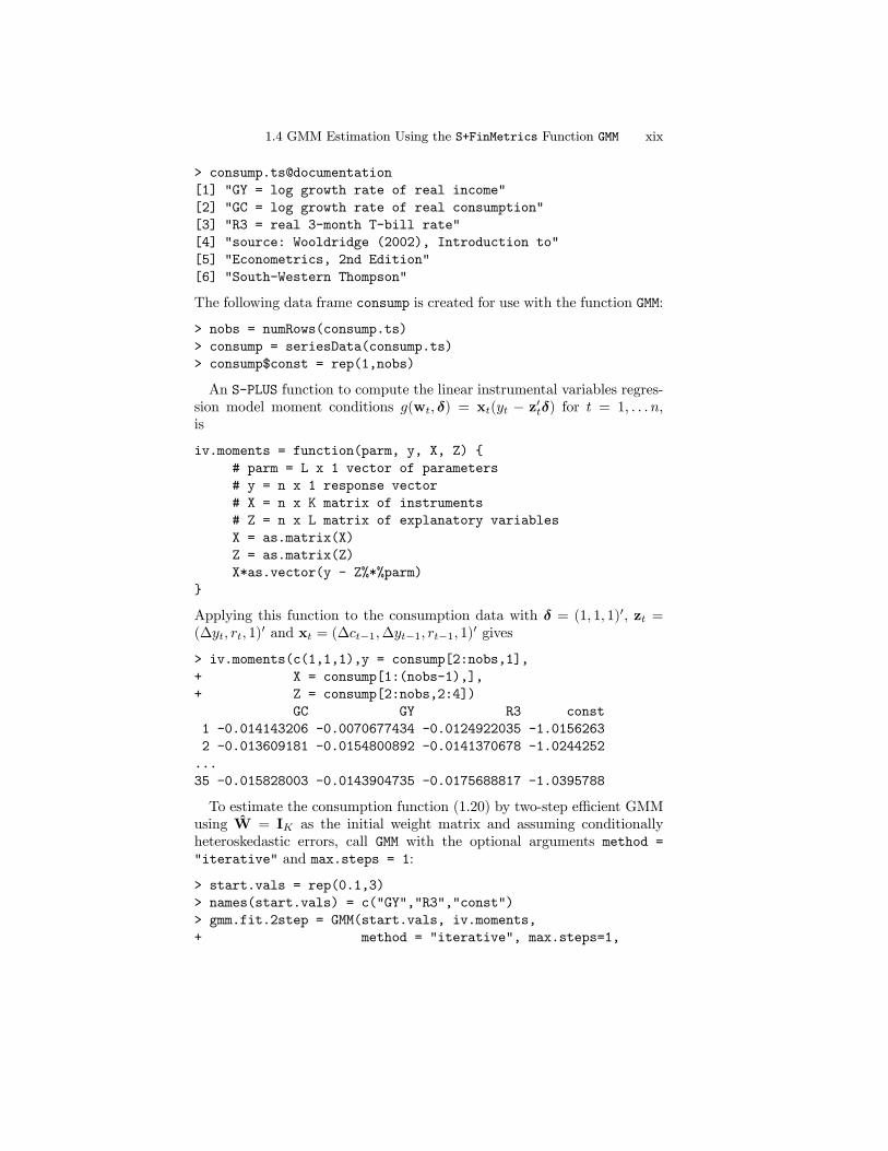
> consump.ts@documentation

[1] "GY = log growth rate of real income"

[2] "GC = log growth rate of real consumption"

[3] "R3 = real 3-month T-bill rate"

[4] "source: Wooldridge (2002), Introduction to"

[5] "Econometrics, 2nd Edition"

[6] "South-Western Thompson"

The following data frame consump is created for use with the function GMM:

> nobs = numRows(consump.ts)

> consump = seriesData(consump.ts)

> consump$const = rep(1,nobs)

An S-PLUS function to compute the linear instrumental variables regres-sion model moment conditions g(wt, δ) = xt(yt − z0tδ) for t = 1, . . . n,is

iv.moments = function(parm, y, X, Z) {

# parm = L x 1 vector of parameters

# y = n x 1 response vector

# X = n x K matrix of instruments

# Z = n x L matrix of explanatory variables

X = as.matrix(X)

Z = as.matrix(Z)

X*as.vector(y - Z%*%parm)

}

Applying this function to the consumption data with δ = (1, 1, 1)0, zt =(∆yt, rt, 1)

0 and xt = (∆ct−1,∆yt−1, rt−1, 1)0 gives

> iv.moments(c(1,1,1),y = consump[2:nobs,1],

+ X = consump[1:(nobs-1),],

+ Z = consump[2:nobs,2:4])

GC GY R3 const

1 -0.014143206 -0.0070677434 -0.0124922035 -1.0156263

2 -0.013609181 -0.0154800892 -0.0141370678 -1.0244252

...

35 -0.015828003 -0.0143904735 -0.0175688817 -1.0395788

To estimate the consumption function (1.20) by two-step efficient GMMusing W = IK as the initial weight matrix and assuming conditionallyheteroskedastic errors, call GMM with the optional arguments method ="iterative" and max.steps = 1:

> start.vals = rep(0.1,3)

> names(start.vals) = c("GY","R3","const")

> gmm.fit.2step = GMM(start.vals, iv.moments,

+ method = "iterative", max.steps=1,

xx 1. Generalized Method of Moments

+ y = consump[2:nobs,1],



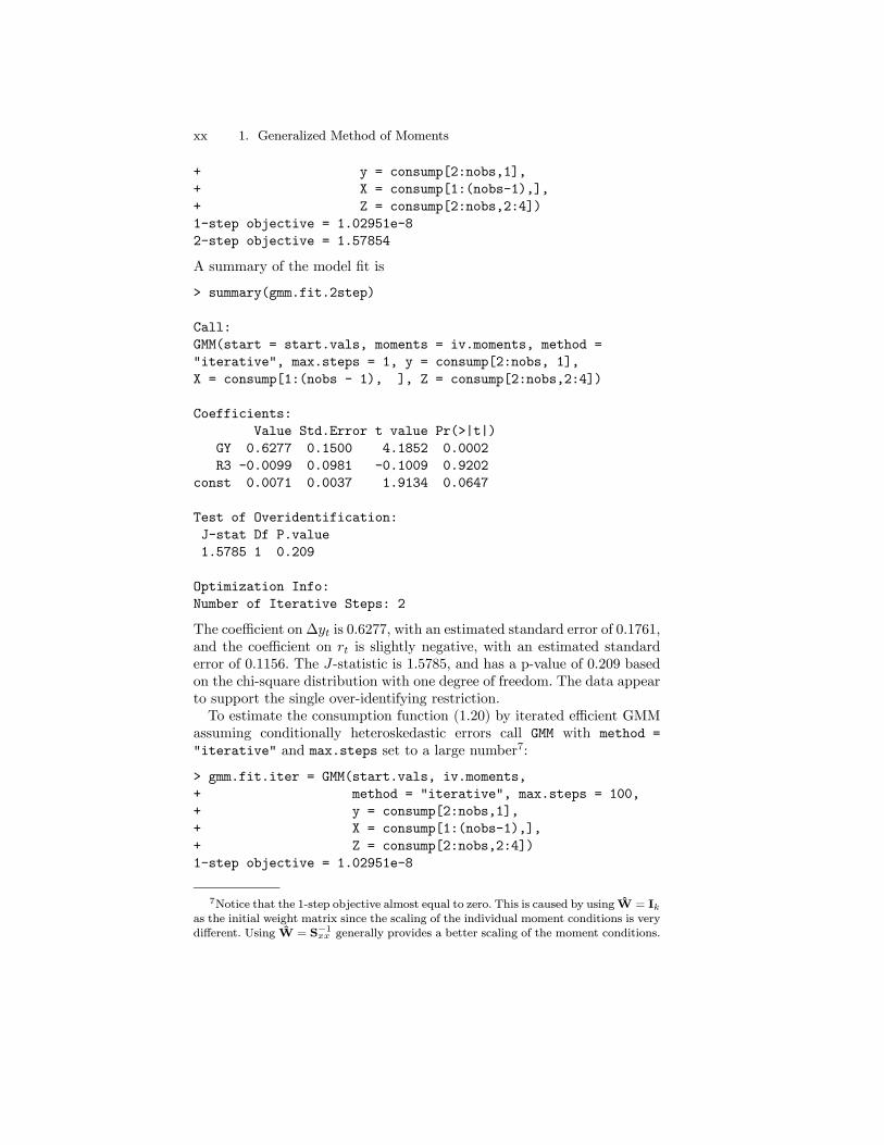
1-step objective = 1.02951e-8

2-step objective = 1.57854

A summary of the model fit is

> summary(gmm.fit.2step)

Call:

GMM(start = start.vals, moments = iv.moments, method =

"iterative", max.steps = 1, y = consump[2:nobs, 1],

X = consump[1:(nobs - 1), ], Z = consump[2:nobs,2:4])

Coefficients:


GY 0.6277 0.1500 4.1852 0.0002

R3 -0.0099 0.0981 -0.1009 0.9202

const 0.0071 0.0037 1.9134 0.0647


J-stat Df P.value

1.5785 1 0.209

Optimization Info:

Number of Iterative Steps: 2

The coefficient on∆yt is 0.6277, with an estimated standard error of 0.1761,and the coefficient on rt is slightly negative, with an estimated standarderror of 0.1156. The J-statistic is 1.5785, and has a p-value of 0.209 basedon the chi-square distribution with one degree of freedom. The data appearto support the single over-identifying restriction.To estimate the consumption function (1.20) by iterated efficient GMM

assuming conditionally heteroskedastic errors call GMM with method =

"iterative" and max.steps set to a large number7:

> gmm.fit.iter = GMM(start.vals, iv.moments,

+ method = "iterative", max.steps = 100,





7Notice that the 1-step objective almost equal to zero. This is caused by using W = Ikas the initial weight matrix since the scaling of the individual moment conditions is verydifferent. Using W = S−1xx generally provides a better scaling of the moment conditions.

1.4 GMM Estimation Using the S+FinMetrics Function GMM xxi


...


To compute the continuously updated efficient GMM estimator (1.14),call GMM with method = "simultaneous":

> start.vals = gmm.fit.iter$parameters

> gmm.fit.cu = GMM(start.vals, iv.moments,

+ method = "simultaneous",




Good starting values are important for the CU estimator, and the aboveestimation uses the iterated GMM estimates as starting values.Finally, to compute an inefficient 1-step GMM estimator with W = I4

use



> gmm.fit.1step = GMM(start.vals, iv.moments,


+ w = diag(4), w0.efficient = F,






Warning messages:

1: Maximum iterative steps exceeded. in: GMM(start.vals,

iv.moments, method = "iterative", max.steps = ....

2: The J-Statistic is not valid since the weight matrix is

not efficient. in: GMM(start.vals, iv.moments, method

= "iterative", max.steps = ....

Table 1.2 summarizes the different efficient GMM estimators for the pa-rameters in (1.20). The results are very similar across the efficient estima-tions8.

Example 3 Estimating the instrumental variables regression model usingTSLS

8To match the default Eviews output for GMM, set the optional argumentdf.correction=F.

xxii 1. Generalized Method of Moments

∆ct = δ1 + δ2∆yt + δ3rt + εtxt = (1,∆ct−1,∆yt−1, rt−1)0, E[xtεt] = 0, E[xtx0tε2t ] = SEstimator δ1 δ2 δ3 J − stat

2-step efficient.007(.004)

.627(.150)

−.010(.098)

1.578(.209)

Iterated efficient.008(.004)

.591(.144)

−.032(.095)

1.855(.173)

CU efficient.008(.003)

.574(.139)

−.054.095

1.747(.186)

1-step inefficient.003(.005)

.801(.223)

−.024(.116)

−−

TABLE 1.2. Efficient GMM estimates of the consumption function parameters.

The TSLS estimator of δ may be computed using the function GMM bysupplying the fixed weight matrixW = S−1xx as follows

9

> w.tsls = crossprod(consump[1:(nobs-1),])/nobs



> gmm.fit.tsls = GMM(start.vals,iv.moments,

+ method = "iterative",max.steps = 0,

+ w = w.tsls,w0.efficient = T,





Warning messages:

Maximum iterative steps exceeded. in: GMM(start.vals,

iv.moments, method = "iterative", max.steps = ....

> gmm.fit.tsls

Call:


"iterative", w = w.tsls, max.steps = 0, w0.efficient

= T, y = consump[2:nobs, 1], X = consump[1:(nobs -1), ],

Z = consump[2:nobs, 2:4])

Coefficients:

GY R3 const

0.5862 -0.0269 0.0081


9Recall, the GMM function uses the inverse of w as the weight matrix.

1.4 GMM Estimation Using the S+FinMetrics Function GMM xxiii

J-stat Df P.value

0.0001 1 0.9915

Optimization Info:


The TSLS estimate of δ is similar to the efficient iterated estimate. TheJ−statistic and the estimate of avar(δTSLS) computed using W = S−1xx ,however, are not correct since S−1xx is proportional to the efficient weightmatrix. To get the correct values for these quantities a consistent estimateσ2 of σ2 is required to form the efficient weight matrix σ2S−1xx . This is easilyaccomplished using

# compute TSLS estimate of error variance

> y = as.vector(consump[2:nobs,1])

> X = as.matrix(consump[1:(nobs-1),])

> Z = as.matrix(consump[2:nobs,2:4])

> d.hat = coef(gmm.fit.tsls)

> e.hat = y - Z%*%d.hat

> df = nrow(Z) - ncol(Z)

> s2 = as.numeric(crossprod(e.hat)/df)

# compute correct efficient weight matrix for tsls

# that contains error variance term

> w.tsls2 = crossprod(X)*s2/nobs



> gmm.fit.tsls2 = GMM(start.vals,iv.moments,

+ method = "iterative",max.steps = 0,

+ w = w.tsls2,w0.efficient = T,





> summary(gmm.fit.tsls2)

Call:


"iterative", w = w.tsls2, max.steps = 0, w0.efficient

= T, y = consump[2:nobs, 1], X = consump[1:(nobs -1), ],

Z = consump[2:nobs, 2:4])

Coefficients:


GY 0.5862 0.1327 4.4177 0.0001

R3 -0.0269 0.0753 -0.3576 0.7230

xxiv 1. Generalized Method of Moments

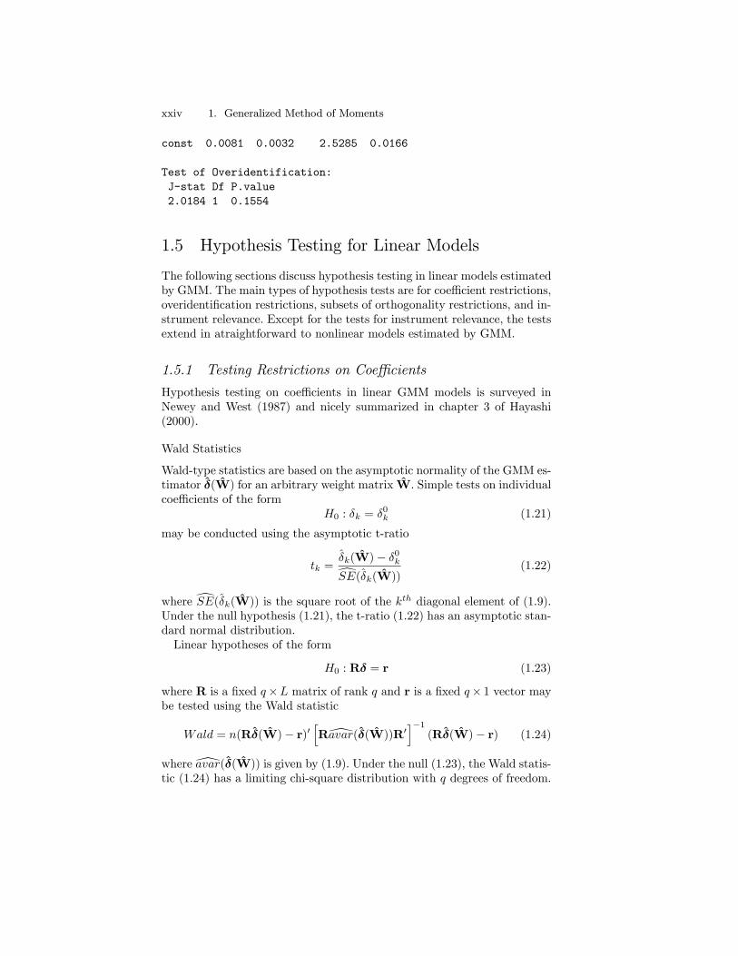
const 0.0081 0.0032 2.5285 0.0166


J-stat Df P.value

2.0184 1 0.1554

1.5 Hypothesis Testing for Linear Models

The following sections discuss hypothesis testing in linear models estimatedby GMM. The main types of hypothesis tests are for coefficient restrictions,overidentification restrictions, subsets of orthogonality restrictions, and in-strument relevance. Except for the tests for instrument relevance, the testsextend in atraightforward to nonlinear models estimated by GMM.

1.5.1 Testing Restrictions on Coefficients

Hypothesis testing on coefficients in linear GMM models is surveyed inNewey and West (1987) and nicely summarized in chapter 3 of Hayashi(2000).

Wald Statistics

Wald-type statistics are based on the asymptotic normality of the GMM es-timator δ(W) for an arbitrary weight matrix W. Simple tests on individualcoefficients of the form

H0 : δk = δ0k (1.21)

may be conducted using the asymptotic t-ratio

tk =δk(W)− δ0kdSE(δk(W))

(1.22)

wheredSE(δk(W)) is the square root of the kth diagonal element of (1.9).Under the null hypothesis (1.21), the t-ratio (1.22) has an asymptotic stan-dard normal distribution.Linear hypotheses of the form

H0 : Rδ = r (1.23)

where R is a fixed q×L matrix of rank q and r is a fixed q× 1 vector maybe tested using the Wald statistic

Wald = n(Rδ(W)− r)0hR[avar(δ(W))R0

i−1(Rδ(W)− r) (1.24)

where[avar(δ(W)) is given by (1.9). Under the null (1.23), the Wald statis-tic (1.24) has a limiting chi-square distribution with q degrees of freedom.

1.5 Hypothesis Testing for Linear Models xxv

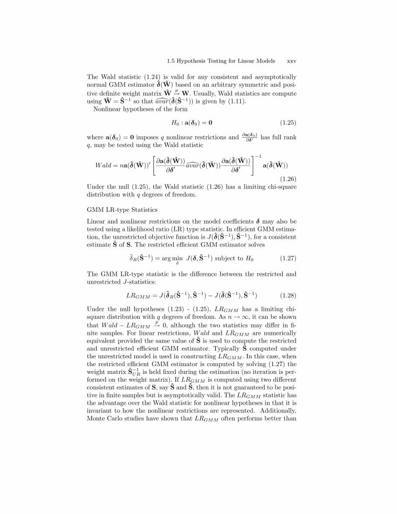
The Wald statistic (1.24) is valid for any consistent and asymptoticallynormal GMM estimator δ(W) based on an arbitrary symmetric and posi-

tive definite weight matrix Wp→W. Usually, Wald statistics are compute

using W = S−1 so that [avar(δ(S−1)) is given by (1.11).Nonlinear hypotheses of the form

H0 : a(δ0) = 0 (1.25)

where a(δ0) = 0 imposes q nonlinear restrictions and∂a(δ0)∂δ 0 has full rank

q, may be tested using the Wald statistic

Wald = na(δ(W))0"∂a(δ(W))

∂δ0[avar(δ(W))

∂a(δ(W))

∂δ0

#−1a(δ(W))

(1.26)Under the null (1.25), the Wald statistic (1.26) has a limiting chi-squaredistribution with q degrees of freedom.

GMM LR-type Statistics

Linear and nonlinear restrictions on the model coefficients δ may also betested using a likelihood ratio (LR) type statistic. In efficient GMM estima-tion, the unrestricted objective function is J(δ(S−1), S−1), for a consistentestimate S of S. The restricted efficient GMM estimator solves

δR(S−1) = argmin

δJ(δ, S−1) subject to H0 (1.27)

The GMM LR-type statistic is the difference between the restricted andunrestricted J-statistics:

LRGMM = J(δR(S−1), S−1)− J(δ(S−1), S−1) (1.28)

Under the null hypotheses (1.23) - (1.25), LRGMM has a limiting chi-square distribution with q degrees of freedom. As n→∞, it can be shown

that Wald − LRGMMp→ 0, although the two statistics may differ in fi-

nite samples. For linear restrictions, Wald and LRGMM are numericallyequivalent provided the same value of S is used to compute the restrictedand unrestricted efficient GMM estimator. Typically S computed underthe unrestricted model is used in constructing LRGMM . In this case, whenthe restricted efficient GMM estimator is computed by solving (1.27) theweight matrix S−1UR is held fixed during the estimation (no iteration is per-formed on the weight matrix). If LRGMM is computed using two differentconsistent estimates of S, say S and S, then it is not guaranteed to be posi-tive in finite samples but is asymptotically valid. The LRGMM statistic hasthe advantage over the Wald statistic for nonlinear hypotheses in that it isinvariant to how the nonlinear restrictions are represented. Additionally,Monte Carlo studies have shown that LRGMM often performs better than

xxvi 1. Generalized Method of Moments

Wald in finite samples. In particular, Wald tends to over reject the nullwhen it is true.

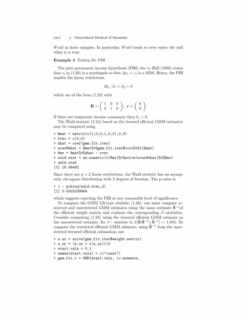
Example 4 Testing the PIH

The pure permanent income hypothesis (PIH) due to Hall (1980) statesthat ct in (1.20) is a martingale so that ∆ct = εt is a MDS. Hence, the PIHimplies the linear restrictions

H0 : δ1 = δ2 = 0

which are of the form (1.23) with

R =

µ1 0 00 1 0

¶, r =

µ00

¶If there are temporary income consumers then δ1 > 0.The Wald statistic (1.24) based on the iterated efficient GMM estimator

may be computed using

> Rmat = matrix(c(1,0,0,1,0,0),2,3)

> rvec = c(0,0)

> dhat = coef(gmm.fit.iter)

> avarRbhat = Rmat%*%gmm.fit.iter$vcov%*%t(Rmat)

> Rmr = Rmat%*%dhat - rvec

> wald.stat = as.numeric(t(Rmr)%*%solve(avarRbhat)%*%Rmr)

> wald.stat

[1] 16.99482

Since there are q = 2 linear restrictions, the Wald statistic has an asymp-totic chi-square distribution with 2 degrees of freedom. The p-value is

> 1 - pchisq(wald.stat,2)

[1] 0.0002039964

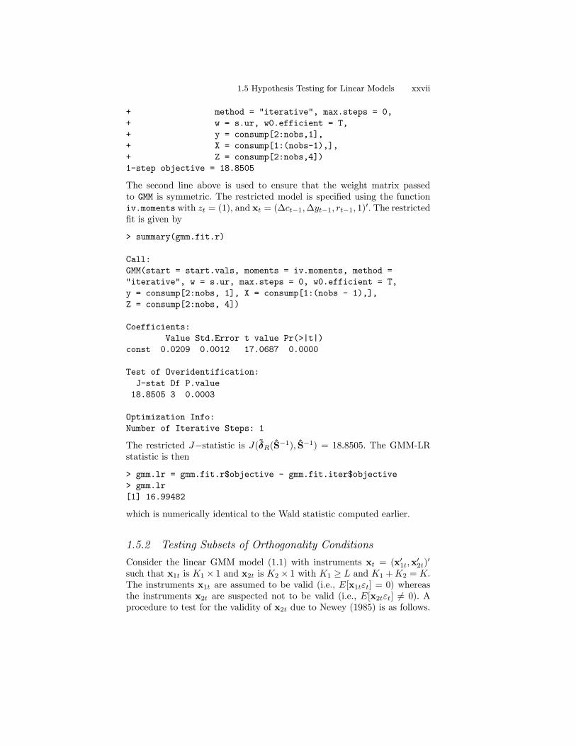
which suggests rejecting the PIH at any reasonable level of significance.To compute the GMM LR-type statistic (1.28), one must compute re-

stricted and unrestricted GMM estimates using the same estimate S−1ofthe efficient weight matrix and evaluate the corresponding J−statistics.Consider computing (1.28) using the iterated efficient GMM estimate asthe unrestricted estimate. Its J− statistic is J(δ(S−1), S−1) = 1.855. Tocompute the restricted efficient GMM estimate, using S−1 from the unre-stricted iterated efficient estimation, use

> s.ur = solve(gmm.fit.iter$weight.matrix)

> s.ur = (s.ur + t(s.ur))/2

> start.vals = 0.1

> names(start.vals) = c("const")

> gmm.fit.r = GMM(start.vals, iv.moments,

1.5 Hypothesis Testing for Linear Models xxvii


+ w = s.ur, w0.efficient = T,



+ Z = consump[2:nobs,4])


The second line above is used to ensure that the weight matrix passedto GMM is symmetric. The restricted model is specified using the functioniv.moments with zt = (1), and xt = (∆ct−1,∆yt−1, rt−1, 1)0. The restrictedfit is given by

> summary(gmm.fit.r)

Call:


"iterative", w = s.ur, max.steps = 0, w0.efficient = T,

y = consump[2:nobs, 1], X = consump[1:(nobs - 1),],

Z = consump[2:nobs, 4])

Coefficients:


const 0.0209 0.0012 17.0687 0.0000


J-stat Df P.value

18.8505 3 0.0003

Optimization Info:


The restricted J−statistic is J(δR(S−1), S−1) = 18.8505. The GMM-LRstatistic is then

> gmm.lr = gmm.fit.r$objective - gmm.fit.iter$objective

> gmm.lr

[1] 16.99482

which is numerically identical to the Wald statistic computed earlier.

1.5.2 Testing Subsets of Orthogonality Conditions

Consider the linear GMM model (1.1) with instruments xt = (x01t,x02t)

0

such that x1t is K1 × 1 and x2t is K2 × 1 with K1 ≥ L and K1 +K2 = K.The instruments x1t are assumed to be valid (i.e., E[x1tεt] = 0) whereasthe instruments x2t are suspected not to be valid (i.e., E[x2tεt] 6= 0). Aprocedure to test for the validity of x2t due to Newey (1985) is as follows.

xxviii 1. Generalized Method of Moments

First, estimate (1.1) by efficient GMM using the full set of instruments xtgiving

δ(S−1Full) = (S0xzS−1FullSxz)

−1S0xzS−1FullSxy

where

SFull =

·S11,Full S12,FullS21,Full S22,Full

¸such that S11,Full is K1 × K1. Second, estimate (1.1) by efficient GMM

using only the instruments x1t and using the weight matrix S−111,Full giving

δ(S−111,Full) = (S0x1zS

−111,FullSx1z)

−1S0x1zS−111,FullSx1y

Next, form the statistic10

C = J(δ(S−1Full), S−1Full)− J(δ(S−111,Full), S

−111,Full) (1.29)

Under the null hypothesis that E[xtεt] = 0, the statistic C has a limitingchi-square distribution with K −K1 degrees of freedom.

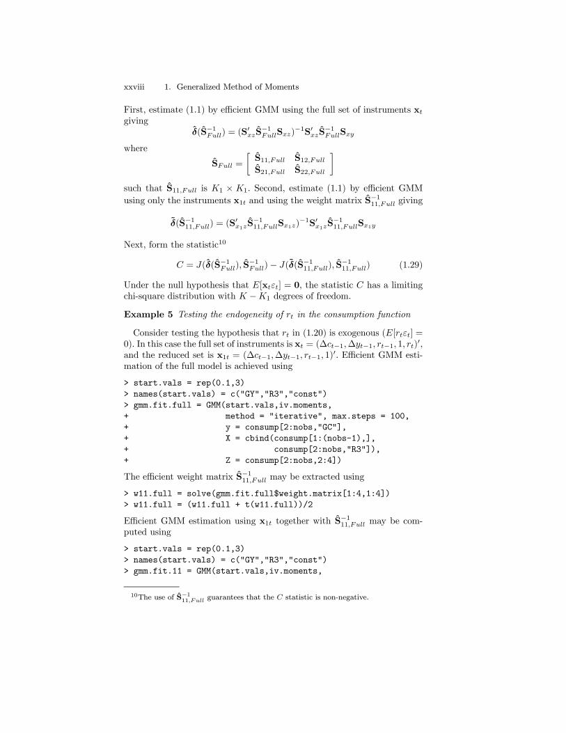
Example 5 Testing the endogeneity of rt in the consumption function

Consider testing the hypothesis that rt in (1.20) is exogenous (E[rtεt] =0). In this case the full set of instruments is xt = (∆ct−1,∆yt−1, rt−1, 1, rt)0,and the reduced set is x1t = (∆ct−1,∆yt−1, rt−1, 1)0. Efficient GMM esti-mation of the full model is achieved using



> gmm.fit.full = GMM(start.vals,iv.moments,


+ y = consump[2:nobs,"GC"],

+ X = cbind(consump[1:(nobs-1),],

+ consump[2:nobs,"R3"]),


The efficient weight matrix S−111,Full may be extracted using

> w11.full = solve(gmm.fit.full$weight.matrix[1:4,1:4])

> w11.full = (w11.full + t(w11.full))/2

Efficient GMM estimation using x1t together with S−111,Full may be com-

puted using



> gmm.fit.11 = GMM(start.vals,iv.moments,

10The use of S−111,Full guarantees that the C statistic is non-negative.

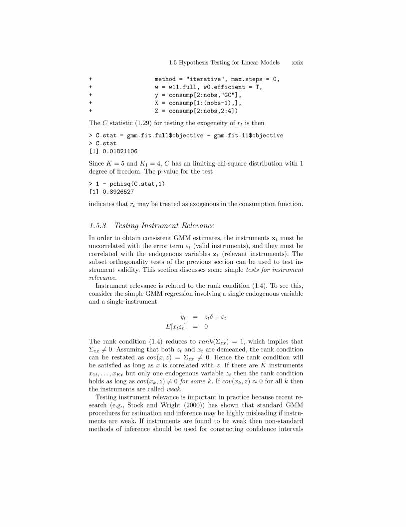
1.5 Hypothesis Testing for Linear Models xxix


+ w = w11.full, w0.efficient = T,

+ y = consump[2:nobs,"GC"],



The C statistic (1.29) for testing the exogeneity of rt is then

> C.stat = gmm.fit.full$objective - gmm.fit.11$objective

> C.stat

[1] 0.01821106

Since K = 5 and K1 = 4, C has an limiting chi-square distribution with 1degree of freedom. The p-value for the test

> 1 - pchisq(C.stat,1)

[1] 0.8926527

indicates that rt may be treated as exogenous in the consumption function.

1.5.3 Testing Instrument Relevance

In order to obtain consistent GMM estimates, the instruments xt must beuncorrelated with the error term εt (valid instruments), and they must becorrelated with the endogenous variables zt (relevant instruments). Thesubset orthogonality tests of the previous section can be used to test in-strument validity. This section discusses some simple tests for instrumentrelevance.Instrument relevance is related to the rank condition (1.4). To see this,

consider the simple GMM regression involving a single endogenous variableand a single instrument

yt = ztδ + εt

E[xtεt] = 0

The rank condition (1.4) reduces to rank(Σzx) = 1, which implies thatΣzx 6= 0. Assuming that both zt and xt are demeaned, the rank conditioncan be restated as cov(x, z) = Σzx 6= 0. Hence the rank condition willbe satisfied as long as x is correlated with z. If there are K instrumentsx1t, . . . , xKt but only one endogenous variable zt then the rank conditionholds as long as cov(xk, z) 6= 0 for some k. If cov(xk, z) ≈ 0 for all k thenthe instruments are called weak.Testing instrument relevance is important in practice because recent re-

search (e.g., Stock and Wright (2000)) has shown that standard GMMprocedures for estimation and inference may be highly misleading if instru-ments are weak. If instruments are found to be weak then non-standardmethods of inference should be used for constucting confidence intervals

xxx 1. Generalized Method of Moments

and performing hypothesis tests. Stock, Wright and Yogo (2002) give anice survey of the issues associated with using GMM in the presence ofweak instruments, and discuss the non-standard inference procedures thatshould be used.In the general linear GMM regression (1.1), the relevance of the set of

instruments xt for each endogenous variable in zt can be tested as follows.First, let z1t denote the L1×1 vector of non-constant endogenous variablesin zt, and let x1t denote the K1 × 1 remaining deterministic or exogenousvariables in zt such that zt = (z

01t,x

01t)

0 and L1+K1 = L. Similarly, definex2t as the K2 × 1 vector of exogenous variables that are excluded fromzt. so that xt = (x

01t,x

02t)

0 and K1 +K2 = K. What is important for therank condition are the correlations between the endogenous variables inz1t and the instruments in x2t. To measure these correlations and to testfor instrument relevance, estimate by least squares the so-called first stageregression

z1lt = x01tπ1l + x2tπ2l + vlt, l = 1, . . . , L1

for each endogenous variable in z1t. The t-ratios on the variables in x2tcan be used to assess the strength of the correlation between z1lt and thevariables in x2t. The F-statistic for testing π2l = 0 can be used to assessthe joint relevance of x2t for z1lt.

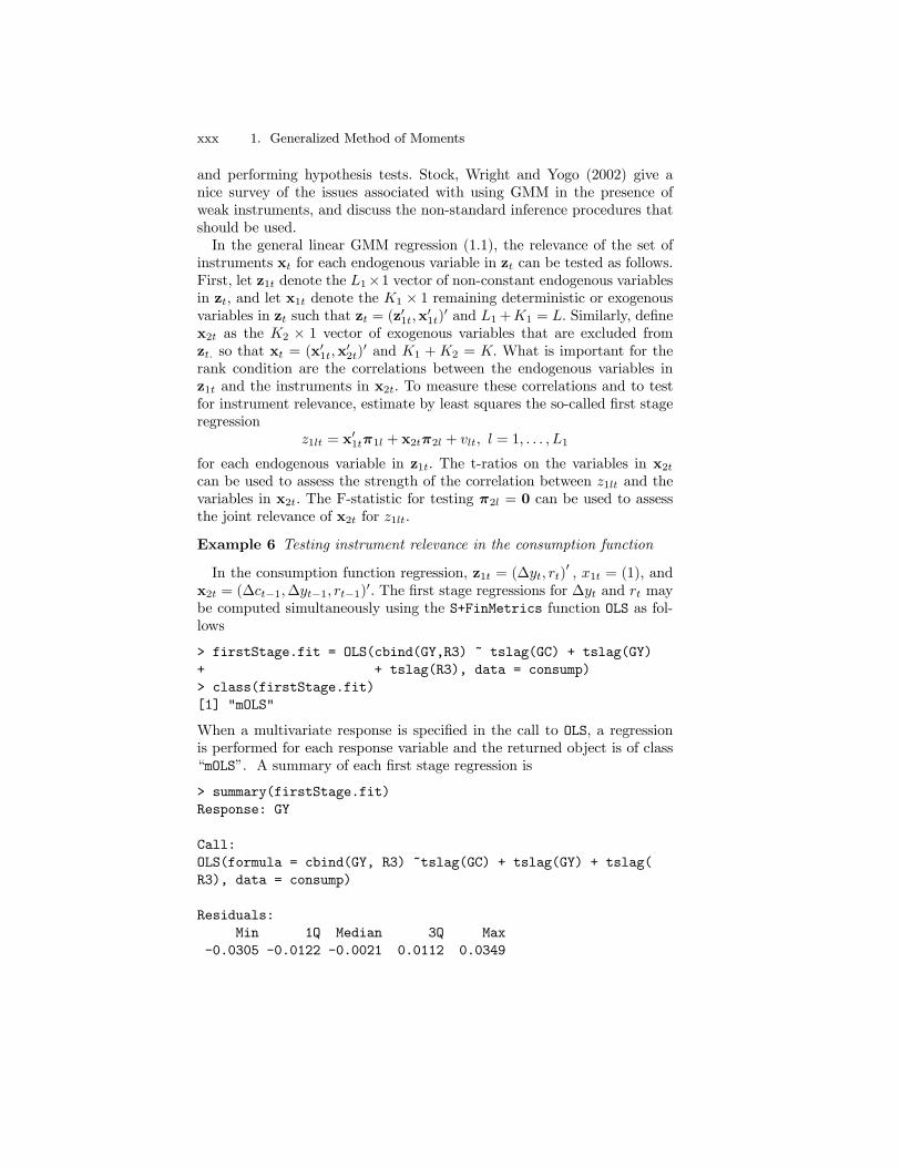
Example 6 Testing instrument relevance in the consumption function

In the consumption function regression, z1t = (∆yt, rt)0 , x1t = (1), and

x2t = (∆ct−1,∆yt−1, rt−1)0. The first stage regressions for ∆yt and rt maybe computed simultaneously using the S+FinMetrics function OLS as fol-lows

> firstStage.fit = OLS(cbind(GY,R3) ~ tslag(GC) + tslag(GY)

+ + tslag(R3), data = consump)

> class(firstStage.fit)

[1] "mOLS"

When a multivariate response is specified in the call to OLS, a regressionis performed for each response variable and the returned object is of class“mOLS”. A summary of each first stage regression is

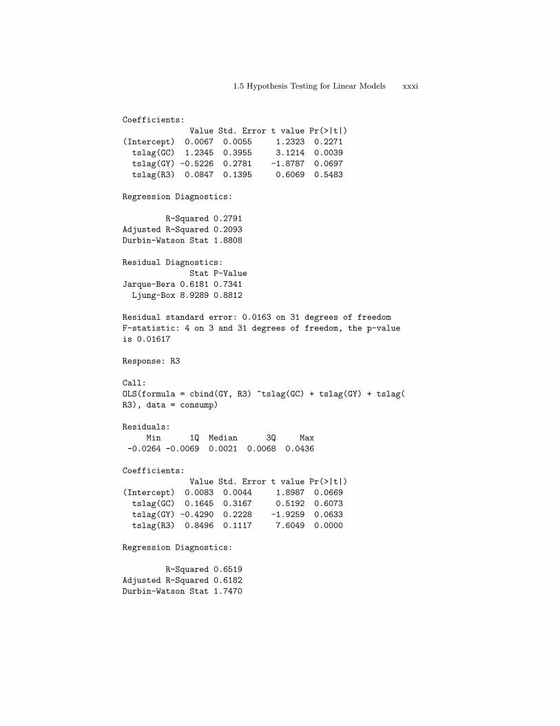
> summary(firstStage.fit)

Response: GY

Call:

OLS(formula = cbind(GY, R3) ~tslag(GC) + tslag(GY) + tslag(

R3), data = consump)

Residuals:


-0.0305 -0.0122 -0.0021 0.0112 0.0349

1.5 Hypothesis Testing for Linear Models xxxi

Coefficients:


(Intercept) 0.0067 0.0055 1.2323 0.2271

tslag(GC) 1.2345 0.3955 3.1214 0.0039

tslag(GY) -0.5226 0.2781 -1.8787 0.0697

tslag(R3) 0.0847 0.1395 0.6069 0.5483

Regression Diagnostics:

R-Squared 0.2791

Adjusted R-Squared 0.2093

Durbin-Watson Stat 1.8808

Residual Diagnostics:

Stat P-Value

Jarque-Bera 0.6181 0.7341

Ljung-Box 8.9289 0.8812

Residual standard error: 0.0163 on 31 degrees of freedom

F-statistic: 4 on 3 and 31 degrees of freedom, the p-value

is 0.01617

Response: R3

Call:

OLS(formula = cbind(GY, R3) ~tslag(GC) + tslag(GY) + tslag(

R3), data = consump)

Residuals:


-0.0264 -0.0069 0.0021 0.0068 0.0436

Coefficients:


(Intercept) 0.0083 0.0044 1.8987 0.0669

tslag(GC) 0.1645 0.3167 0.5192 0.6073

tslag(GY) -0.4290 0.2228 -1.9259 0.0633

tslag(R3) 0.8496 0.1117 7.6049 0.0000

Regression Diagnostics:

R-Squared 0.6519

Adjusted R-Squared 0.6182

Durbin-Watson Stat 1.7470

xxxii 1. Generalized Method of Moments

Residual Diagnostics:

Stat P-Value

Jarque-Bera 14.8961 0.0006

Ljung-Box 20.7512 0.1450

Residual standard error: 0.01305 on 31 degrees of freedom

F-statistic: 19.35 on 3 and 31 degrees of freedom, the p-value

is 2.943e-007

In the first stage regression for ∆yt, the t-ratios for ∆ct−1 and ∆yt−1 aresignificant at the 1% and 10% levels, respectively, indicating that thesevariables are correlated with ∆yt. The F-statistic for testing the joint sig-nificance of the variables in x2t is 4, with a p-value of 0.0167 indicatingthat x2t is relevant for ∆yt.

1.6 Nonlinear GMM

Nonlinear GMM estimation occurs when the K GMM moment conditionsg(wt,θ) are nonlinear functions of the p model parameters θ. Dependingon the model, the moment conditions g(wt,θ) may be K ≥ p nonlinearfunctions satisfying

E[g(wt,θ0)] = 0 (1.30)

Alternatively, for a response variable yt, L explanatory variables zt, and Kinstruments xt, the model may define a nonlinear error term εt

a(yt, zt;θ0) = εt

such thatE[εt] = E[a(yt, zt;θ0)] = 0

Given that xt is orthogonal to εt, define g(wt,θ0) = xtεt = xta(yt, zt;θ0)so that

E[g(wt,θ0)] = E[xtεt] = E[xta(yt, zt;θ0)] = 0 (1.31)

defines the GMM orthogonality conditions.In general, the GMM moment equations (1.30) and (1.31) produce a

system ofK nonlinear equations in p unknowns. Identification of θ0 requiresthat

E[g(wt,θ0)] = 0

E[g(wt,θ)] 6= 0 for θ 6= θ0

and the K × p matrix

G = E

·∂g(wt,θ0)

∂θ0

¸(1.32)

1.6 Nonlinear GMM xxxiii

has full column rank p. The sample moment condition for an arbitrary θ is

gn(θ) = n−1nXt=1

g(wt,θ)

If K = p, then θ0 is apparently just identified and the GMM objectivefunction is

J(θ) = ngn(θ)0gn(θ)

which does not depend on a weight matrix. The corresponding GMM esti-mator is then

θ = argminθ

J(θ)

If K > p, then θ0 is apparently overidentified. Let W denote a K × Ksymmetric and p.d. weight matrix, possibly dependent on the data, such

that Wp→ W as n → ∞ with W symmetric and p.d. Then the GMM

estimator of θ0, denoted θ(W), is defined as

θ(W) = argminθ

J(θ,W) = ngn(θ)0Wgn(θ)

The efficient GMM estimator uses W = S−1such that S

p→S = avar(g).As with efficient GMM estimation of linear models, the efficient GMMestimator of nonlinear models may be computed using a two-step, iterated,or continuous updating estimator.

1.6.1 Asymptotic Properties

Under standard regularity conditions (see Hayashi Chapter 7), it can beshown that

θ(W)p→ θ0

√n³θ(W)− θ0

´d→ N(0, avar(θ(W)))

whereavar(θ(W)) = (G0WG)−1G0WSWG(G0WG)−1 (1.33)

and G is given by (1.32). IfW = S−1 then

avar(θ(S−1)) = (G0S−1G)−1 (1.34)

Notice that with nonlinear GMM, the expression for avar(θ(W)) is of thesame form as in linear GMM except that Σxz = E[xtz

0t] is replaced by

G = Eh∂g(wt,θ0)

∂θ 0

i.

A consistent estimate of avar(θ(W)), denoted[avar(θ(W)),may be com-puted using

[avar(θ(W)) = (G0WG)−1GWSWG(G0WG)−1 (1.35)

xxxiv 1. Generalized Method of Moments

where S is a consistent estimate for S = avar(g) and

G =Gn(θ(W)) = n−1nXt=1

∂g(wt, θ(W))

∂θ0

For the efficient GMM estimator, W = S−1, and

[avar(θ(S−1)) = (G0S−1G)−1 (1.36)

If {gt(wt,θ0)} is an ergodic stationary MDS withE[gt(wt,θ0)gt(wt,θ0)0] =

S, then a consistent estimator of S takes the form

n−1nXt=1

gt(wt, θ)gt(wt, θ)0

where θ is any consistent estimator of θ0. If {gt(wt,θ0)} is a serially cor-related ergodic stationary process then

S = avar(g) = Γ0 + 2∞Xj=1

(Γj + Γ0j)

and the methods discussed in Section 1.3 may be used to consistently esti-mate S.

1.6.2 Hypothesis Tests for Nonlinear Models

Most of the GMM test statistics discussed in the context of linear mod-els have analogues in the context of nonlinear GMM. For example, theJ-statistic for testing the validity of the K moment conditions (1.31) hasthe form (1.15) with the efficient GMM estimate θ(S−1) in place of δ(S−1).The asymptotic null distribution of the J-statistic is chi-squared with K−pdegrees of freedom. Wald statistics for testing linear and non-linear restric-tion on θ have the same form as (1.24) and (1.26), with θ(W) in place ofδ(W). Similarly, GMM LR-type statistics for testing linear and non-linearrestriction on θ have the form (1.28), with θ(S−1) in place of δ(S−1) andwith θ(S−1) in place of δ(S−1). Testing the relevance of instruments innonlinear models, however, is not as straightforward as it is in linear mod-els. In nonlinear models, instruments are relevant if the K × p matrix Gdefined in (1.32) has full column rank p. Testing this condition is problem-atic because G depends on θ0 which is unknown. See Wright (2001) foran approach that can be used to test for instrument relevance in nonlinearmodels.

1.7 Examples of Nonlinear Models xxxv

1.7 Examples of Nonlinear Models

The following sections give detailed examples of estimating nonlinear mod-els using GMM.

1.7.1 Student-t Distribution

As in Hamilton (1994, chapter 14), consider a random sample y1, . . . , yTthat is drawn from a centered Student-t distribution with θ0 degrees offreedom. The density of yt has the form

f(yt; θ0) =Γ[(θ0 + 1)/2]

(πθ0)1/2Γ(θ0/2)[1 + (y2t /θ0)]

−(θ0+1)/2

where Γ(·) is the gamma function. The goal is to estimate the degrees offreedom parameter θ0 by GMM using the moment conditions

E[y2t ] =θ0

θ0 − 2E[y4t ] =

3θ20(θ0 − 2)(θ0 − 4)

which require θ0 > 4. Let wt = (y2t , y

4t )0 and define

g(wt,θ) =

µy2t − θ/(θ − 2)

y4t − 3θ2/(θ − 2)(θ − 4)¶

(1.37)

Then E[g(wt,θ0)] = 0 is the moment condition used for defining the GMMestimator for θ0. Here, K = 2 and p = 1 so θ0 is apparently overidentified.Using the sample moments

gn(θ) =1

n

nXt=1

g(wt, θ) =

µ1n

Pnt=1 y

2t − θ/(θ − 2)

1n

Pnt=1 y

4t − 3θ2/(θ − 2)(θ − 4)

¶the GMM objective function has the form

J(θ) = ngn(θ)0Wgn(θ)

where W is a 2× 2 p.d. and symmetric weight matrix, possibly dependenton the data, such that W

p→W. The efficient GMM estimator uses the

weight matrix S−1 such that Sp→ S = E[g(wt, θ0)g(wt, θ0)

0].A random sample of n = 250 observations from a centered Student-t

distribution with θ0 = 10 degrees of freedom may be generated using theS-PLUS function rt as follows

> set.seed(123)

> y = rt(250,df = 10)

xxxvi 1. Generalized Method of Moments

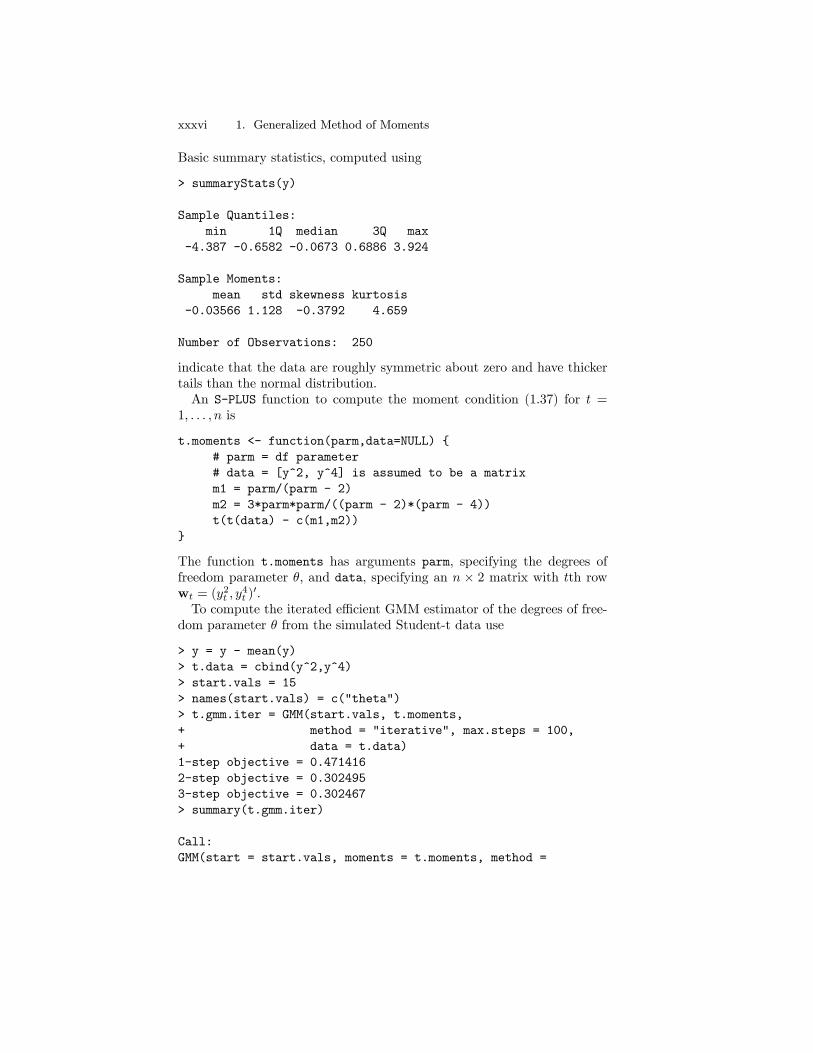
Basic summary statistics, computed using

> summaryStats(y)

Sample Quantiles:

min 1Q median 3Q max

-4.387 -0.6582 -0.0673 0.6886 3.924

Sample Moments:

mean std skewness kurtosis

-0.03566 1.128 -0.3792 4.659

Number of Observations: 250

indicate that the data are roughly symmetric about zero and have thickertails than the normal distribution.An S-PLUS function to compute the moment condition (1.37) for t =

1, . . . , n is

t.moments <- function(parm,data=NULL) {

# parm = df parameter

# data = [y^2, y^4] is assumed to be a matrix

m1 = parm/(parm - 2)

m2 = 3*parm*parm/((parm - 2)*(parm - 4))

t(t(data) - c(m1,m2))

}

The function t.moments has arguments parm, specifying the degrees offreedom parameter θ, and data, specifying an n × 2 matrix with tth rowwt = (y

2t , y

4t )0.

To compute the iterated efficient GMM estimator of the degrees of free-dom parameter θ from the simulated Student-t data use

> y = y - mean(y)

> t.data = cbind(y^2,y^4)

> start.vals = 15

> names(start.vals) = c("theta")

> t.gmm.iter = GMM(start.vals, t.moments,


+ data = t.data)




> summary(t.gmm.iter)

Call:

GMM(start = start.vals, moments = t.moments, method =

1.7 Examples of Nonlinear Models xxxvii

"iterative", max.steps = 100, data = data)

Coefficients:


theta 7.8150 1.1230 6.9592 0.0000


J-stat Df P.value

0.3025 1 0.5823

Optimization Info:


The iterated efficient GMM estimate of θ0 is 7.8150, with an asymptoticstandard error of 1.123. The small J-statistic indicates a correctly specifiedmodel.

1.7.2 MA(1) Model

Following Harris (1999), consider GMM estimation of the parameters inthe MA(1) model

yt = µ0 + εt + ψ0εt−1, t = 1, . . . , n

εt ∼ iid (0, σ20), |ψ0| < 1θ0 = (µ0, ψ0, σ

20)0

Some population moment equations that can be used for GMM estimationare

E[yt] = µ0E[y2t ] = µ20 + σ20(1 + ψ20)

E[ytyt−1] = µ20 + σ20ψ0E[ytyt−2] = µ20

Let wt = (yt, y2t , ytyt−1, ytyt−2)0 and define the moment vector

g(wt,θ) =

yt − µ

y2t − µ2 − σ2(1 + ψ2)ytyt−1 − µ2 − σ2ψ

ytyt−2 − µ2

(1.38)

Then

E[g(wt,θ0)] = 0

xxxviii 1. Generalized Method of Moments

is the population moment condition used for GMM estimation of the modelparameters θ0. The sample moments are

gn(θ) =1

n− 2nXt=3

g(wt,θ) =

1

n−2Pn

t=3 yt − µ1

n−2Pn

t=3 y2t − µ2 − σ2(1 + ψ2)

1n−2

Pnt=3 ytyt−1 − µ2 − σ2ψ

1n−2

Pnt=3 ytyt−2 − µ2

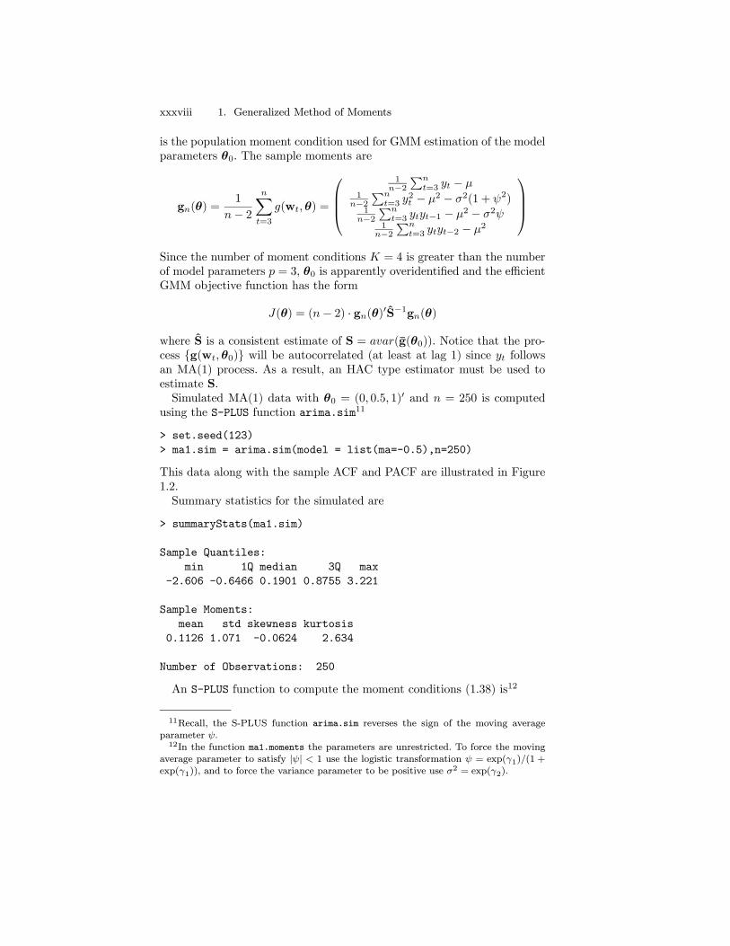
Since the number of moment conditions K = 4 is greater than the numberof model parameters p = 3, θ0 is apparently overidentified and the efficientGMM objective function has the form

J(θ) = (n− 2) · gn(θ)0S−1gn(θ)

where S is a consistent estimate of S = avar(g(θ0)). Notice that the pro-cess {g(wt,θ0)} will be autocorrelated (at least at lag 1) since yt followsan MA(1) process. As a result, an HAC type estimator must be used toestimate S.Simulated MA(1) data with θ0 = (0, 0.5, 1)0 and n = 250 is computed

using the S-PLUS function arima.sim11

> set.seed(123)

> ma1.sim = arima.sim(model = list(ma=-0.5),n=250)

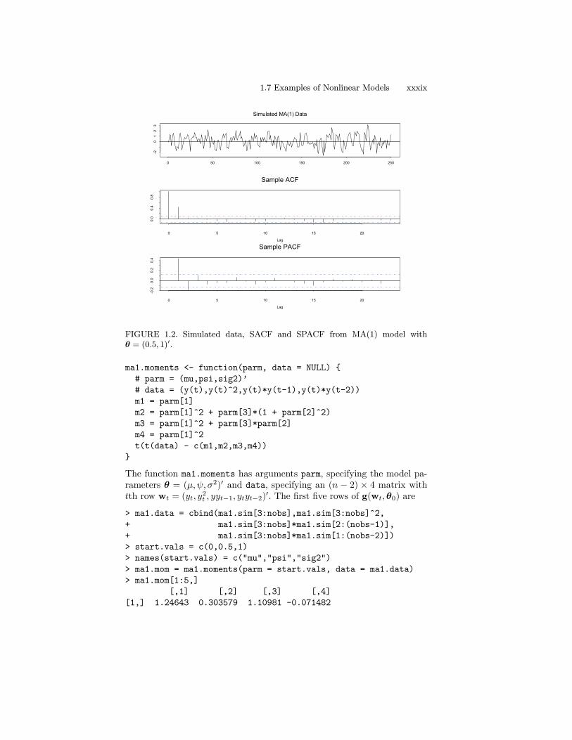
This data along with the sample ACF and PACF are illustrated in Figure1.2.Summary statistics for the simulated are

> summaryStats(ma1.sim)

Sample Quantiles:


-2.606 -0.6466 0.1901 0.8755 3.221

Sample Moments:


0.1126 1.071 -0.0624 2.634


An S-PLUS function to compute the moment conditions (1.38) is12

11Recall, the S-PLUS function arima.sim reverses the sign of the moving averageparameter ψ.12In the function ma1.moments the parameters are unrestricted. To force the moving

average parameter to satisfy |ψ| < 1 use the logistic transformation ψ = exp(γ1)/(1 +exp(γ1)), and to force the variance parameter to be positive use σ

2 = exp(γ2).

1.7 Examples of Nonlinear Models xxxix

Simulated MA(1) Data

0 50 100 150 200 250

-20

12

3

Lag

0 5 10 15 20

0.0

0.4

0.8

Sample ACF

Lag

0 5 10 15 20

-0.2

0.0

0.2

0.4

Sample PACF

FIGURE 1.2. Simulated data, SACF and SPACF from MA(1) model withθ = (0.5, 1)0.

ma1.moments <- function(parm, data = NULL) {

# parm = (mu,psi,sig2)’

# data = (y(t),y(t)^2,y(t)*y(t-1),y(t)*y(t-2))

m1 = parm[1]

m2 = parm[1]^2 + parm[3]*(1 + parm[2]^2)

m3 = parm[1]^2 + parm[3]*parm[2]

m4 = parm[1]^2

t(t(data) - c(m1,m2,m3,m4))

}

The function ma1.moments has arguments parm, specifying the model pa-rameters θ = (µ,ψ, σ2)0 and data, specifying an (n − 2) × 4 matrix withtth row wt = (yt, y

2t , yyt−1, ytyt−2)0. The first five rows of g(wt,θ0) are

> ma1.data = cbind(ma1.sim[3:nobs],ma1.sim[3:nobs]^2,

+ ma1.sim[3:nobs]*ma1.sim[2:(nobs-1)],

+ ma1.sim[3:nobs]*ma1.sim[1:(nobs-2)])

> start.vals = c(0,0.5,1)

> names(start.vals) = c("mu","psi","sig2")

> ma1.mom = ma1.moments(parm = start.vals, data = ma1.data)

> ma1.mom[1:5,]

[,1] [,2] [,3] [,4]

[1,] 1.24643 0.303579 1.10981 -0.071482

xl 1. Generalized Method of Moments

Series 1

ACF

0 5 10 15

0.0

0.2

0.4

0.6

0.8

1.0

Series 1 and Series 2

0 5 10 15

-0.1

0-0

.05

0.0

0.05

0.10


0 5 10 15

-0.1

0-0

.05

0.0

0.05

0.10

0.15


0 5 10 15

-0.1

0.0

0.1

0.2


ACF

-15 -10 -5 0

-0.1

5-0

.10

-0.0

50.

00.

050.

10

Series 2

0 5 10 15

0.0

0.2

0.4

0.6

0.8

1.0


0 5 10 15

0.0

0.2

0.4

0.6


0 5 10 15

-0.1

5-0

.10

-0.0

50.

00.

050.

100.

15


ACF

-15 -10 -5 0

-0.1

0.0

0.1

0.2


-15 -10 -5 0

0.0

0.2

0.4

0.6

Series 3

0 5 10 15

0.0

0.2

0.4

0.6

0.8

1.0


0 5 10 15

-0.1

0.0

0.1

0.2

0.3


Lag

ACF

-15 -10 -5 0

-0.1

0.0

0.1

0.2


Lag-15 -10 -5 0

-0.1

0-0

.05

0.0

0.05

0.10

0.15

0.20


Lag-15 -10 -5 0

-0.1

0.0

0.1

0.2

0.3

Series 4

Lag0 5 10 15

0.0

0.2

0.4

0.6

0.8

1.0

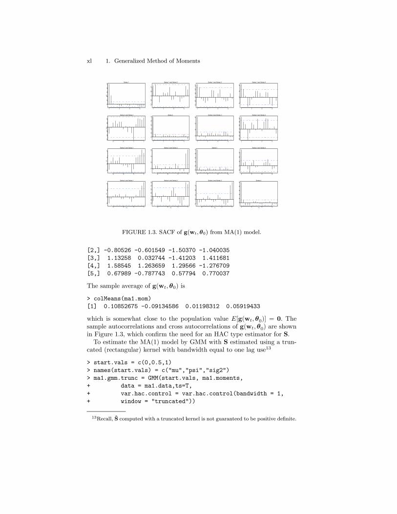
FIGURE 1.3. SACF of g(wt, θ0) from MA(1) model.

[2,] -0.80526 -0.601549 -1.50370 -1.040035

[3,] 1.13258 0.032744 -1.41203 1.411681

[4,] 1.58545 1.263659 1.29566 -1.276709

[5,] 0.67989 -0.787743 0.57794 0.770037

The sample average of g(wt,θ0) is

> colMeans(ma1.mom)

[1] 0.10852675 -0.09134586 0.01198312 0.05919433

which is somewhat close to the population value E[g(wt,θ0)] = 0. Thesample autocorrelations and cross autocorrelations of g(wt,θ0) are shownin Figure 1.3, which confirm the need for an HAC type estimator for S.To estimate the MA(1) model by GMM with S estimated using a trun-

cated (rectangular) kernel with bandwidth equal to one lag use13

> start.vals = c(0,0.5,1)

> names(start.vals) = c("mu","psi","sig2")

> ma1.gmm.trunc = GMM(start.vals, ma1.moments,

+ data = ma1.data,ts=T,

+ var.hac.control = var.hac.control(bandwidth = 1,

+ window = "truncated"))

13Recall, S computed with a truncated kernel is not guaranteed to be positive definite.

1.7 Examples of Nonlinear Models xli




The fitted results are

> summary(ma1.gmm.trunc)

Call:

GMM(start = start.vals, moments = ma1.moments, ts = T,

var.hac.control = var.hac.control(bandwidth = 1,

window = "truncated"), data = ma1.data)

Coefficients:


mu 0.1018 0.0927 1.0980 0.2733

psi 0.5471 0.0807 6.7788 0.0000

sig2 0.8671 0.0763 11.3581 0.0000


J-stat Df P.value

0.3549 1 0.5513

Optimization Info:


The GMM estimate of µ0 is close to the sample mean, the estimate of ψ0is slightly larger than 0.5 and the estimate of σ20 is slightly smaller than 1.The low J−statistic indicates a correctly specified model.To illustrate the impact of model mis-specification on GMM estimation,

consider fitting an MA(1) model by GMM to data simulated from an AR(1)model

yt − µ0 = φ0(yt−1 − µ0) + εt, εt ∼ iid N(0, σ20)

The AR(1) model has moments

E[yt] = µ0

E[y2t ] = µ20 + σ20/(1− φ20)

E[ytyt−1] = µ20 + φσ20/(1− φ20)

E[ytyt−2] = µ20 + φ2σ20/(1− φ20)

Simulated AR(1) data with µ0 = 0, φ0 = 0.5, σ20 = 1 and n = 250 iscomputed using the S-PLUS function arima.sim

> set.seed(123)

> ar1.sim = arima.sim(model=list(ar=0.5),n=250)

The moment data required for GMM estimation of the MA(1) model are

xlii 1. Generalized Method of Moments

> nobs = numRows(ar1.sim)

> ar1.data = cbind(ar1.sim[3:nobs],ar1.sim[3:nobs]^2,

+ ar1.sim[3:nobs]*ar1.sim[2:(nobs-1)],

+ ar1.sim[3:nobs]*ar1.sim[1:(nobs-2)])

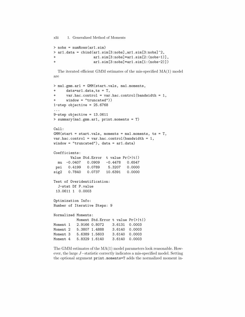
The iterated efficient GMM estimates of the mis-specified MA(1) modelare

> ma1.gmm.ar1 = GMM(start.vals, ma1.moments,

+ data=ar1.data,ts = T,

+ var.hac.control = var.hac.control(bandwidth = 1,

+ window = "truncated"))


...


> summary(ma1.gmm.ar1, print.moments = T)

Call:

GMM(start = start.vals, moments = ma1.moments, ts = T,

var.hac.control = var.hac.control(bandwidth = 1,

window = "truncated"), data = ar1.data)

Coefficients:


mu -0.0407 0.0909 -0.4478 0.6547

psi 0.4199 0.0789 5.3207 0.0000

sig2 0.7840 0.0737 10.6391 0.0000


J-stat Df P.value

13.0611 1 0.0003

Optimization Info:


Normalized Moments:

Moment Std.Error t value Pr(>|t|)

Moment 1 2.9166 0.8072 3.6131 0.0003

Moment 2 5.3807 1.4888 3.6140 0.0003

Moment 3 5.6389 1.5603 3.6140 0.0003

Moment 4 5.8329 1.6140 3.6140 0.0003

The GMM estimates of the MA(1) model parameters look reasonable. How-ever, the large J−statistic correctly indicates a mis-specified model. Settingthe optional argument print.moments=T adds the normalized moment in-

1.7 Examples of Nonlinear Models xliii

formation to the summary output. Since the J−statistic is large, all of thenormalized moments are significantly different from zero.

1.7.3 Euler Equation Asset Pricing Model

Following Hansen and Singleton (1982), a representative agent is assumedto choose an optimal consumption path by maximizing the present dis-counted value of lifetime utility from consumption

max∞Xt=1

E£βt0U(Ct)|It

¤subject to the budget constraint

Ct + PtQt ≤ VtQt−1 +Wt

where It denotes the information available at time t, Ct denotes real con-sumption at t, Wt denotes real labor income at t, Pt denotes the price of apure discount bond maturing at time t + 1 that pays Vt+1, Qt representsthe quantity of bonds held at t, and β0 represents a time discount factor.The first order condition for the maximization problem may be representedas the conditional moment equation (Euler equation)

E

·(1 +Rt+1)β0

U 0(Ct+1)

U 0(Ct)|It¸− 1 = 0

where 1 + Rt+1 =Vt+1Vt

is the gross return on the bond at time t + 1.Assuming utility has the power form

U(C) =C1−α0

1− α0

where α0 represents the intertemporal rate of substitution (risk aversion),then

U 0(Ct+1)

U 0(Ct)=

µCt+1

Ct

¶−α0and the conditional moment equation becomes

E

"(1 +Rt+1)β0

µCt+1

Ct

¶−α0|It#− 1 = 0 (1.39)

Define the nonlinear error term as

εt+1 = a(Rt+1, Ct+1/Ct;α0, β0) = (1 +Rt+1)β0

µCt+1

Ct

¶−α0− 1

= a(zt+1,θ0)

xliv 1. Generalized Method of Moments

with zt+1 = (Rt+1, Ct+1/Ct)0 and θ0 = (α0, β0)

0. Then the conditionalmoment equation (1.39) may be represented as

E[εt+1|It] = E[a(zt+1,θ0)|It] = 0Since {εt+1, It+1} is a MDS, potential instruments xt include current andlagged values of the elements in zt as well as a constant. For example, onecould use

xt = (1, Ct/Ct−1, Ct−1/Ct−2, Rt, Rt−1)0

Since xt ⊂ It, the conditional moment (1.39) implies that

E[xtεt+1|It] = E[xta(zt+1,θ0)|It] = 0and by the law of total expectations

E[xtεt+1] = 0

For GMM estimation, define the nonlinear residual as

et+1 = (1 +Rt+1)β

µCt+1

Ct

¶−α− 1

and form the vector of moments

g(wt+1,θ) = xtet+1 = xta(zt+1,θ) (1.40)

=

(1 +Rt+1)β³Ct+1Ct

´−α− 1

(Ct/Ct−1)µ(1 +Rt+1)β

³Ct+1Ct

´−α− 1¶

(Ct−1/Ct−2)µ(1 +Rt+1)β

³Ct+1Ct

´−α− 1¶

Rt

µ(1 +Rt+1)β

³Ct+1Ct

´−α− 1¶

Rt−1

µ(1 +Rt+1)β

³Ct+1Ct

´−α− 1¶

In (1.40) there are K = 5 moment conditions to identify L = 2 model pa-rameters givingK−L = 3 overidentifying restrictions. The GMM objectivefunction is

J(θ, S−1) = (n− 2) · gn(θ)0S−1gn(θ)where S is a consistent estimate of S = avar(g).An S-PLUS function to compute the Euler moments (1.40) is

euler1.moments <- function(parm, data = NULL) {

# parm = (beta,gamma)

# data = (1+R(t+1),C(t+1)/C(t),1,C(t)/C(t-1),

# C(t-1)/C(t-2),R(t),R(t-1),...)

1.7 Examples of Nonlinear Models xlv

ncol = numCols(data)

euler = data[,1]*parm[1]*(data[,2]^(-parm[2])) - 1

as.matrix(rep(euler,(ncol-2))*data[,3:ncol])

}

The function euler1.moments has arguments parm, specifying the modelparameters θ = (β, α)0 and data, specifying an (n− 2)× 7 matrix with tthrow wt+1 = (1 +Rt+1, Ct+1/Ct, 1, Ct/Ct−1, Ct−1/Ct−2, Rt, Rt−1)0.Verbeek (2000) (chapter 5, section 7) describes an extension of the model

presented above that allows the individual to invest in J risky assets withreturns Rj,t+1 (j = 1, . . . , J), as well as a risk-free asset with certain returnRf,t+1. Assuming power utility, and restricting attention to unconditionalmoments (i.e., using xt = 1), the Euler equations may be written as

E

"(1 +Rf,t+1)β0

µCt+1

Ct

¶−α0#− 1 = 0 (1.41)

E

"(Rj,t+1 −Rf,t+1)β0

µCt+1

Ct

¶−α0#= 0, j = 1, . . . , J

Define the stochastic discount factor as

mt+1(θ0) = β0

µCt+1

Ct

¶−α0so that the risky assets satisfy

E[(Rj,t+1 −Rf,t+1) ·mt+1(θ0)] = 0

Using the identity E[xy] = cov(x, y) + E[x]E[y], the risk premium for therisky assets may be deduced as

E[Rj,t+1 −Rf,t+1] = −cov(mt+1(θ0), Rj,t+1 −Rf,t+1)

E[mt+1(θ0)](1.42)

If the asset pricing model is correct then right-hand-side of (1.42) shouldexplain the cross sectional variation of expected returns across assets.For GMM estimation define the J + 1 vector of moments

g(wt+1,θ) =

(1 +Rf,t+1)β³Ct+1Ct

´−α− 1

(R1,t+1 −Rf,t+1)β³Ct+1Ct

´−α...

(RJ,t+1 −Rf,t+1)β³Ct+1Ct

´−α

An S-PLUS function to compute the above moments is

xlvi 1. Generalized Method of Moments

euler2.moments <- function(parm, data = NULL) {


# data = (C(t+1)/C(t),1+Rf(t+1),R1(t+1)-Rf(t+1),...,

# RJ(t+1)-Rf(t+1))


sdf = parm[1]*data[,1]^(-parm[2])

d1 = (sdf - 1)*data[,2]

d2 = as.matrix(rep(sdf,(ncol-2))*data[,3:ncol])

cbind(d1,d2)

}

The function euler2.moments has arguments parm, specifying the modelparameters θ = (β, α)0 and data, specifying an n× (J +1) matrix with tthrow wt+1 = (Ct+1/Ct, 1 +Rf,t+1, R1,t+1 −Rf,t+1, . . . , RJ,t+1 −Rf,t+1)

0.Following Verbeek (2000), the power utility asset pricing model is esti-

mated using monthly data over the period February 1959 through Novem-ber 199314. Ten size-based portfolios from the Center for Research in Secu-rity Prices (CRSP) data base are used as the risky assets. That is, portfolio1 contains the monthly returns on the smallest 10% of firms (by marketcapitalization) listed on the New York Stock Exchange, and portfolio 10contains the returns on the largest 10% of firms. The risk-free asset isthe monthly return on 3-month U.S. T-Bills, and real consumption is mea-sured by total U.S. personal consumption expenditures on nondurables andservices. The data is available in the S+FinMetrics “timeSeries” objectpricing.ts, which has variables

> colIds(pricing.ts)

[1] "CONS" "R1" "R2" "R3" "R4" "R5" "R6" "R7"

[9] "R8" "R9" "R10" "RF"

The data to be passed to the function euler2.moments is constructed using

> pricing.mat = as.matrix(seriesData(pricing.ts))

> ncol = numCols(pricing.mat)

> excessRet.mat = apply(pricing.mat[,2:(ncol-1)], 2,

+ function(x,y){x-y},

+ pricing.mat[,"RF"])


# RJ(t+1)-Rf(t+1))

> euler.data = cbind(pricing.mat[,"CONS"],

+ 1 + pricing.mat[,"RF"],

+ excessRet.mat)

The iterated efficient GMM estimator may be computed using

14The data is taken from Manro Verbeek’s web page athttp://www.econ.kuleuven.ac.be/GME.

1.7 Examples of Nonlinear Models xlvii

> start.vals = c(1,5)

> names(start.vals) = c("beta","alpha")

> euler.gmm.fit = GMM(start.vals, euler2.moments,

+ method = "iterative",data = euler.data)

> summary(euler.gmm.fit)

Call:

GMM(start = start.vals, moments = euler2.moments, method =

"iterative", data = euler.data)

Coefficients:


beta 0.8314 0.1170 7.1049 0.0000

alpha 57.4020 34.3021 1.6734 0.0950


J-stat Df P.value

5.6574 9 0.7737

Optimization Info:


The small J-statistic indicates a correctly specified model. The estimateof the time discount parameter β is economically reasonable and fairlyprecise, but the estimate of the risk aversion parameter α is implausiblylarge and imprecise. The large estimate of α illustrates the well knownequity premium puzzle under which the high risk premia on equity assetsis associated with extremely risk averse investors.The 1-step inefficient GMM estimator withW = I11 may be computed

using

> euler.gmm.fit2 = GMM(start.vals, euler2.moments,


+ w = diag(11), w0.efficient = F,

+ data = euler.data)

> summary(euler.gmm.fit2)

Call:

GMM(start = start.vals, moments = euler2.moments, method =

"iterative", w = diag(11), max.steps = 0, w0.efficient

= F, data = euler.data)

Coefficients:


beta 0.7031 0.1446 4.8612 0.0000

alpha 91.4097 38.2102 2.3923 0.0172

xlviii 1. Generalized Method of Moments

The usual J−statistic is not valid for the 1-step estimates so it is notreported. The 1-step estimates are similar to the iterated efficient GMMestimates, and have slightly larger estimated standard errors.Cochrane (1996, 2001) recommends using the 1-step GMM estimates

to compute empirical pricing errors based on (1.42), since these estimatesminimize such pricing errors by construction. The pricing errors can thenbe plotted to evaluate the economic significance of the proposed asset pric-ing model. The empirical pricing errors may be computed and plotted asfollows. First, the historical average excess returns on the ten portfolios arecomputed using

> excessRet.hat = colMeans(excessRet.mat)

Next, the average excess returns on the ten portfolios predicted by themodel, based on the 1-step inefficient GMM estimates, may be computedusing the function

predRet <- function(parm,data) {



# RJ(t+1)-Rf(t+1))


sdf = parm[1]*data[,1]^(-parm[2])

tmp <- function(x,y) { -var(x,y)/mean(y) }

ans = apply(data[,3:ncol], 2, FUN = tmp,sdf)

ans

}

> predRet.hat = predRet(coef(euler.gmm.fit2),euler.data)

Figure 1.4 shows the historical average excess returns and the predictedaverage excess returns along with a 450 line.If the model is correct then all points should lie on the 450 line. The plotshows that the model under-predicts the small firm excess returns andover-predicts the large firm excess returns.

1.7.4 Stochastic Volatility Model

The simple log-normal stochastic volatility (SV) model, due to Taylor(1986), is given by

yt = σtZt, t = 1, . . . , n (1.43)

lnσ2t = ω0 + β0 lnσ2t−1 + σ0,uut

(Zt, ut)0 ∼ iid N(0, I2)

θ0 = (ω0, β0, σ0,u)0

For 0 < β0 < 1 and σ0,u ≥ 0 the series yt is strictly stationary and ergodic,and unconditional moments of all orders exist. In the SV model, the series

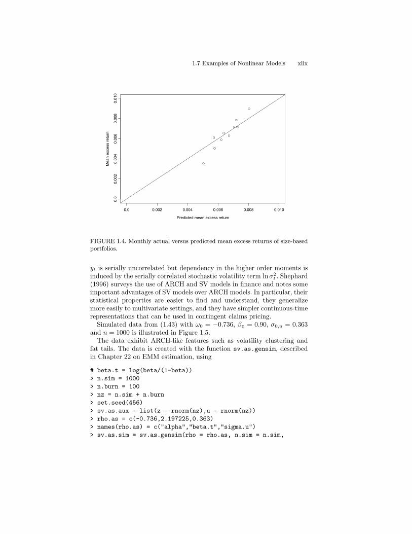
1.7 Examples of Nonlinear Models xlix

Predicted mean excess return

Mea

n ex

cess

retu

rn

0.0 0.002 0.004 0.006 0.008 0.010

0.0

0.00

20.

004

0.00

60.

008

0.01

0

FIGURE 1.4. Monthly actual versus predicted mean excess returns of size-basedportfolios.

yt is serially uncorrelated but dependency in the higher order moments isinduced by the serially correlated stochastic volatility term lnσ2t . Shephard(1996) surveys the use of ARCH and SV models in finance and notes someimportant advantages of SV models over ARCH models. In particular, theirstatistical properties are easier to find and understand, they generalizemore easily to multivariate settings, and they have simpler continuous-timerepresentations that can be used in contingent claims pricing.Simulated data from (1.43) with ω0 = −0.736, β0 = 0.90, σ0,u = 0.363

and n = 1000 is illustrated in Figure 1.5.The data exhibit ARCH-like features such as volatility clustering and

fat tails. The data is created with the function sv.as.gensim, describedin Chapter 22 on EMM estimation, using

# beta.t = log(beta/(1-beta))

> n.sim = 1000

> n.burn = 100

> nz = n.sim + n.burn

> set.seed(456)

> sv.as.aux = list(z = rnorm(nz),u = rnorm(nz))

> rho.as = c(-0.736,2.197225,0.363)

> names(rho.as) = c("alpha","beta.t","sigma.u")

> sv.as.sim = sv.as.gensim(rho = rho.as, n.sim = n.sim,

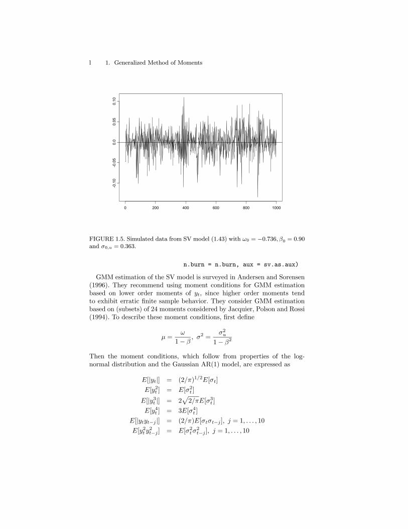
l 1. Generalized Method of Moments

0 200 400 600 800 1000

-0.1

0-0

.05

0.0

0.05

0.10

FIGURE 1.5. Simulated data from SV model (1.43) with ω0 = −0.736, β0 = 0.90and σ0,u = 0.363.

n.burn = n.burn, aux = sv.as.aux)

GMM estimation of the SV model is surveyed in Andersen and Sorensen(1996). They recommend using moment conditions for GMM estimationbased on lower order moments of yt, since higher order moments tendto exhibit erratic finite sample behavior. They consider GMM estimationbased on (subsets) of 24 moments considered by Jacquier, Polson and Rossi(1994). To describe these moment conditions, first define

µ =ω

1− β, σ2 =

σ2u1− β2

Then the moment conditions, which follow from properties of the log-normal distribution and the Gaussian AR(1) model, are expressed as

E[|yt|] = (2/π)1/2E[σt]

E[y2t ] = E[σ2t ]

E[|y3t |] = 2p2/πE[σ3t ]

E[y4t ] = 3E[σ4t ]

E[|ytyt−j |] = (2/π)E[σtσt−j ], j = 1, . . . , 10E[y2t y

2t−j ] = E[σ2tσ

2t−j ], j = 1, . . . , 10

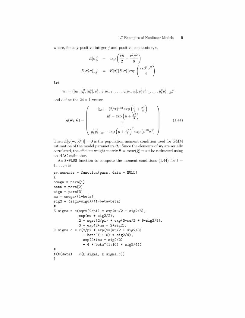
1.7 Examples of Nonlinear Models li

where, for any positive integer j and positive constants r, s,

E[σrt ] = exp

µrµ

2+

r2σ2

8

¶E[σrtσ

st−j ] = E[σrt ]E[σ

st ] exp

Ãrsβjσ2

4

!Let

wt = (|yt|, y2t , |y3t |, y4t , |ytyt−1|, . . . , |ytyt−10|, y2t y2t−1, . . . , y2t y2t−10)0

and define the 24× 1 vector

g(wt,θ) =

|yt|− (2/π)1/2 exp

³µ2 +

σ2

8

´y2t − exp

³µ+ σ2

2

´...

y2t y2t−10 − exp

³µ+ σ2

2

´2exp

¡β10σ2

¢

(1.44)

Then E[g(wt,θ0)] = 0 is the population moment condition used for GMMestimation of the model parameters θ0. Since the elements ofwt are seriallycorrelated, the efficient weight matrix S = avar(g) must be estimated usingan HAC estimator.An S-PLUS function to compute the moment conditions (1.44) for t =

1, . . . , n is

sv.moments = function(parm, data = NULL)

{

omega = parm[1]

beta = parm[2]

sigu = parm[3]

mu = omega/(1-beta)

sig2 = (sigu*sigu)/(1-beta*beta)

#

E.sigma = c(sqrt(2/pi) * exp(mu/2 + sig2/8),

exp(mu + sig2/2),

2 * sqrt(2/pi) * exp(3*mu/2 + 9*sig2/8),

3 * exp(2*mu + 2*sig2))

E.sigma.c = c(2/pi * exp(2*(mu/2 + sig2/8)

+ beta^(1:10) * sig2/4),

exp(2*(mu + sig2/2)

+ 4 * beta^(1:10) * sig2/4))

#

t(t(data) - c(E.sigma, E.sigma.c))

}

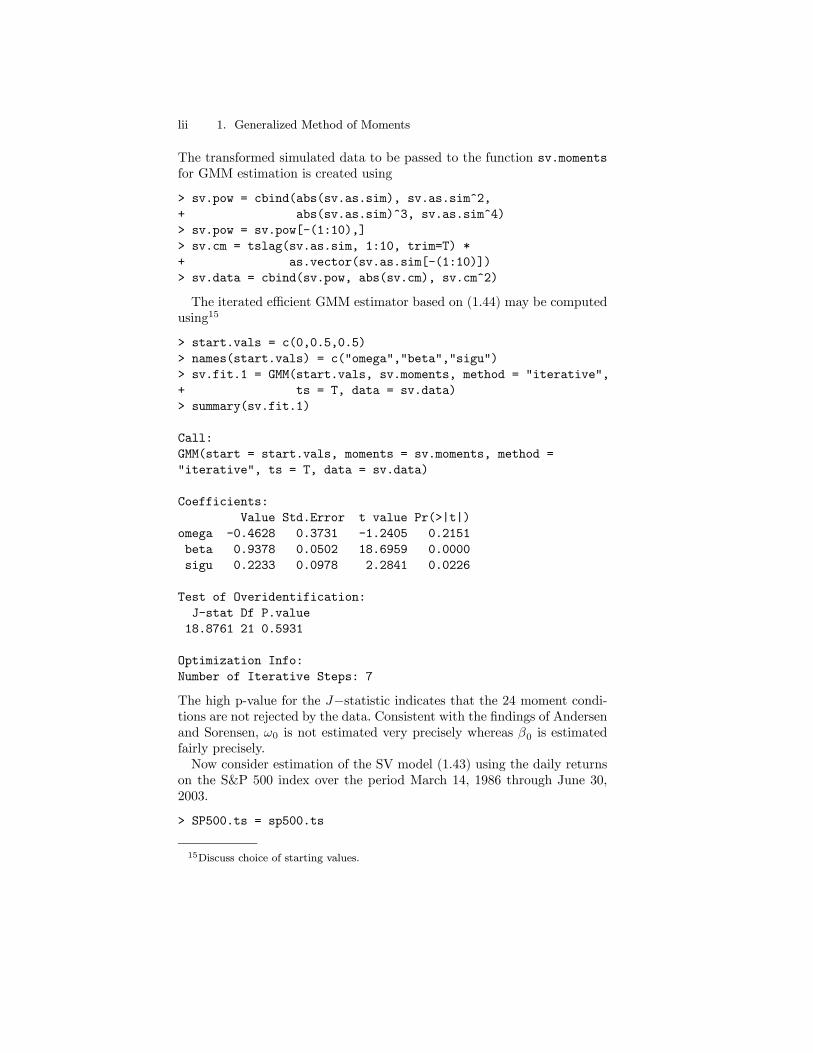
lii 1. Generalized Method of Moments

The transformed simulated data to be passed to the function sv.momentsfor GMM estimation is created using

> sv.pow = cbind(abs(sv.as.sim), sv.as.sim^2,

+ abs(sv.as.sim)^3, sv.as.sim^4)

> sv.pow = sv.pow[-(1:10),]

> sv.cm = tslag(sv.as.sim, 1:10, trim=T) *

+ as.vector(sv.as.sim[-(1:10)])

> sv.data = cbind(sv.pow, abs(sv.cm), sv.cm^2)

The iterated efficient GMM estimator based on (1.44) may be computedusing15

> start.vals = c(0,0.5,0.5)

> names(start.vals) = c("omega","beta","sigu")

> sv.fit.1 = GMM(start.vals, sv.moments, method = "iterative",

+ ts = T, data = sv.data)

> summary(sv.fit.1)

Call:

GMM(start = start.vals, moments = sv.moments, method =

"iterative", ts = T, data = sv.data)

Coefficients:


omega -0.4628 0.3731 -1.2405 0.2151

beta 0.9378 0.0502 18.6959 0.0000

sigu 0.2233 0.0978 2.2841 0.0226


J-stat Df P.value

18.8761 21 0.5931

Optimization Info:


The high p-value for the J−statistic indicates that the 24 moment condi-tions are not rejected by the data. Consistent with the findings of Andersenand Sorensen, ω0 is not estimated very precisely whereas β0 is estimatedfairly precisely.Now consider estimation of the SV model (1.43) using the daily returns

on the S&P 500 index over the period March 14, 1986 through June 30,2003.

> SP500.ts = sp500.ts

15Discuss choice of starting values.

1.7 Examples of Nonlinear Models liii

> SP500.ts@data = as.matrix(seriesData(sp500.ts))

>

> SP500.pow = seriesMerge(abs(SP500.ts), SP500.ts^2,

+ abs(SP500.ts)^3, SP500.ts^4)

> SP500.pow = SP500.pow[-(1:10),]@data

> SP500.cm = tslag(SP500.ts, 1:10, trim=T)@data *

+ as.vector(SP500.ts[-(1:10)]@data)

> SP500.data = cbind(SP500.pow, abs(SP500.cm), SP500.cm^2)

> colIds(SP500.data) = NULL

>

> # iterative GMM estimation of the SV model

> start.vals = c(0,0.5,0.5)

> names(start.vals) = c("omega","beta","sigu")

> sv.fit.SP500 = GMM(start.vals, sv.moments,

+ method = "iterative", ts = T,

+ data = SP500.data)


...


> summary(sv.fit.SP500,print.moments=F)

Call:

GMM(start = start.vals, moments = sv.moments, method =

"iterative", ts = T, data = SP500.data)

Coefficients:


omega -0.1541 0.1758 -0.8767 0.3807

beta 0.9838 0.0184 53.3692 0.0000

sigu 0.1548 0.0908 1.7041 0.0884


J-stat Df P.value

39.9342 21 0.0076

Optimization Info:


The low p-value on the J−statistic indicates that the SV model (1.43) doesnot fit S&P 500 daily returns.

liv 1. Generalized Method of Moments

1.7.5 Interest Rate Diffusion Model

Chan, Karolyi, Longstaff and Sanders (1992), hereafter CKLS, consideredestimating the parameters of the continuous-time interest rate diffusionmodel

drt = (α0 + β0rt)dt+ σ0rγ0t dWt (1.45)

θ0 = (α0, β0, σ0, γ0)0

using GMM. In (1.45), the drift function (α0+β0rt)dtmay be re-parameter-ized as κ0(µ0 − rt)dt where α0 = κ0µ0 and β0 = −κ0. The parameter µ0is the long-run mean, and the parameter κ0 determines the speed of meanreversion. The model (1.45) encompasses a variety of models that have beenproposed for the short-term interest rate. Simulated solutions from (1.45)based on Euler’s method for various models using parameters estimated byCKLS are presented in Chapter 19.CKLS derived moment conditions for GMM estimation of θ0 from the

Euler discretization

rt+∆t − rt = (α0 + β0rt)∆t+ σ0rγ0t

√∆tzt+∆t

E[zt+∆t] = 0, E[z2t+∆t] = 1

They defined the true model error as

εt+∆t = a(rt+∆t − rt, rt;α0, β0, σ0, γ0) = (rt+∆t − rt)− (α0 + β0rt)∆t

= a(zt+∆t,θ0)

where zt+∆t = (rt+∆t − rt, rt)0. Letting It represent information available

at time t, the true error satisfies E[εt+∆t|It] = 0. Since {εt+∆t, It+∆} isa MDS, potential instruments xt include current and lagged values of theelements of zt as well as a constant. As the basis for GMM estimation,CKLS used xt = (1, rt)

0 as the instrument vector and deduced the followingfour conditional moments

E[εt+∆t|It] = 0, E[ε2t+∆t|It] = σ20r2γ0t ∆t

E[εt+∆trt|It] = 0, E[ε2t+∆trt|It] = σ20r2γ0t ∆t · rt

For given values of α and β define the nonlinear residual

et+∆t = (rt+∆t − rt)− (α+ βrt)∆t

and, for wt+∆t = (rt+∆t − rt, rt, r2t )0, define the 4× 1 vector of moments

g(wt+∆t,θ) =

µet+∆te2t+∆t

¶⊗ xt =

et+∆tet+∆trt

e2t+∆t − σ2r2γt ∆t³e2t+∆t − σ2r2γt ∆t

´rt

1.7 Examples of Nonlinear Models lv

Then E[g(wt+∆t,θ0)] = 0 gives the GMM estimating equation. Eventhough {εt, It} is a MDS, the moment vector g(wt,θ0) is likely to be au-tocorrelated since it contains ε2t . For the most general specification (1.45),K = L and the model is just identified. For all models listed in Table ??from Chapter 19, K > L, so that they are overidentified.An S-PLUS function to compute the CKLS moments is

ckls.moments <- function(parm, data = NULL,dt = 1/12) {

# parm = (alpha,beta,sigma,gamma)’

# data = [r(t+dt)-r(t),r(t)]

# dt = discretization step

e.hat = as.vector(data[,1] -

(parm[1] + parm[2]*data[,2])*dt)

m2 = e.hat*as.vector(data[,2])

m3 = e.hat^2 - dt*parm[3]*parm[3]*

(as.vector(data[,2])^(2*parm[4]))

m4 = m3*data[,2]

cbind(e.hat,m2,m3,m4)

}

The function ckls.moments has arguments parm, specifying the model pa-rameters θ = (α, β, σ, γ)0, data, specifying an n × 2 matrix with tth row(rt+∆t − rt, rt), and dt, specifying the discretization increment.GMM estimation is performed on (1.45) using monthly observations on

the U.S. 30-day T-Bill rate over the period June 1964 through November1989. The same data is analyzed in Cliff (2003), and is illustrated in Figure1.6.The data to be passed to the function ckls.moments is constructed using

> data.ckls.ts = seriesMerge(diff(ckls.ts), tslag(ckls.ts))

> colIds(data.ckls.ts)[1] = "RF.diff"

> data.ckls = as.matrix(seriesData(data.ckls.ts))

The summary statistics for ∆rt and rt−1

> summaryStats(data.ckls)

Sample Quantiles:


RF.diff -0.05813 -0.00267 0.0002 0.00324 0.03285

RF.lag1 0.03127 0.04756 0.0603 0.07883 0.16150

Sample Moments:


RF.diff 0.00012 0.008187 -1.347 13.354

RF.lag1 0.06659 0.026375 1.206 4.332

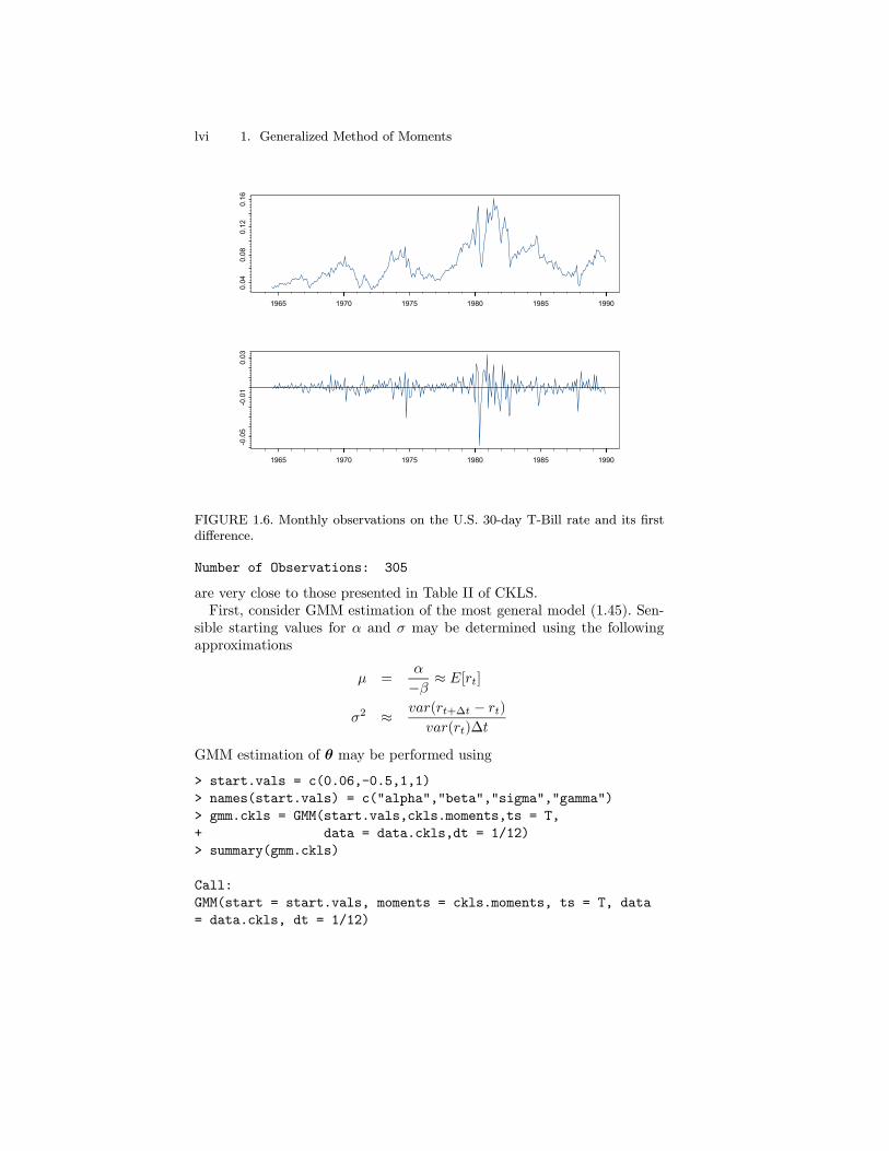
lvi 1. Generalized Method of Moments

1965 1970 1975 1980 1985 1990

0.04

0.08

0.12

0.16

1965 1970 1975 1980 1985 1990

-0.0

5-0

.01

0.03

FIGURE 1.6. Monthly observations on the U.S. 30-day T-Bill rate and its firstdifference.


are very close to those presented in Table II of CKLS.First, consider GMM estimation of the most general model (1.45). Sen-

sible starting values for α and σ may be determined using the followingapproximations

µ =α

−β ≈ E[rt]

σ2 ≈ var(rt+∆t − rt)

var(rt)∆t

GMM estimation of θ may be performed using

> start.vals = c(0.06,-0.5,1,1)

> names(start.vals) = c("alpha","beta","sigma","gamma")

> gmm.ckls = GMM(start.vals,ckls.moments,ts = T,

+ data = data.ckls,dt = 1/12)

> summary(gmm.ckls)

Call:

GMM(start = start.vals, moments = ckls.moments, ts = T, data

= data.ckls, dt = 1/12)

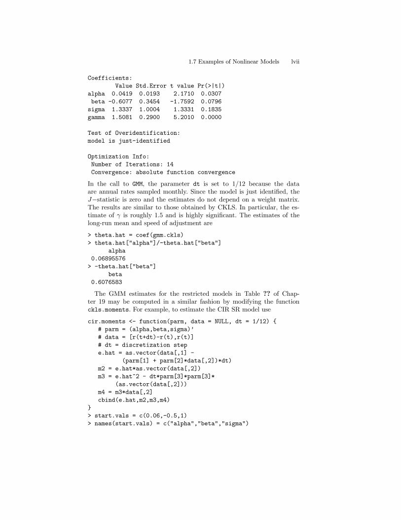
1.7 Examples of Nonlinear Models lvii

Coefficients:


alpha 0.0419 0.0193 2.1710 0.0307

beta -0.6077 0.3454 -1.7592 0.0796

sigma 1.3337 1.0004 1.3331 0.1835

gamma 1.5081 0.2900 5.2010 0.0000



Optimization Info:


Convergence: absolute function convergence

In the call to GMM, the parameter dt is set to 1/12 because the dataare annual rates sampled monthly. Since the model is just identified, theJ−statistic is zero and the estimates do not depend on a weight matrix.The results are similar to those obtained by CKLS. In particular, the es-timate of γ is roughly 1.5 and is highly significant. The estimates of thelong-run mean and speed of adjustment are

> theta.hat = coef(gmm.ckls)

> theta.hat["alpha"]/-theta.hat["beta"]

alpha

0.06895576

> -theta.hat["beta"]

beta

0.6076583

The GMM estimates for the restricted models in Table ?? of Chap-ter 19 may be computed in a similar fashion by modifying the functionckls.moments. For example, to estimate the CIR SR model use

cir.moments <- function(parm, data = NULL, dt = 1/12) {

# parm = (alpha,beta,sigma)’

# data = [r(t+dt)-r(t),r(t)]

# dt = discretization step

e.hat = as.vector(data[,1] -

(parm[1] + parm[2]*data[,2])*dt)

m2 = e.hat*as.vector(data[,2])

m3 = e.hat^2 - dt*parm[3]*parm[3]*

(as.vector(data[,2]))

m4 = m3*data[,2]

cbind(e.hat,m2,m3,m4)

}

> start.vals = c(0.06,-0.5,1)

> names(start.vals) = c("alpha","beta","sigma")

lviii 1. Generalized Method of Moments

> gmm.cir = GMM(start.vals, cir.moments, ts = T,

+ data = data.ckls, dt = 1/12)

> summary(gmm.cir,print.moments = F)

Call:

GMM(start = start.vals, moments = cir.moments, ts = T, data =

data.ckls, dt = 1/12)

Coefficients:


alpha 0.0204 0.0166 1.2258 0.2212

beta -0.2407 0.3023 -0.7963 0.4265

sigma 0.0841 0.0066 12.7661 0.0000


J-stat Df P.value

3.7977 1 0.0513

Optimization Info:


The low p-value on the J−statistic indicates a potentially mis-specifiedmodel.

1.8 References

[1] Andersen, T.G. and B.E. Sorensen (1996). “GMM Estimationof a Stochastic Volatility Model: A Monte Carlo Study,” Journal ofBusiness and Economic Statistics, 14, 328-352.

[2] Brenner, R.J., R.H. Harjes, and K.F. Kroner (1996). “An-other Look at Models of the Short-Term Interest Rate,” Journal ofFinancial and Quantitative Analysis, 31, 85-107.

[3] Campbell, J. and G. Mankiw (1990), “Permanent Income, Cur-rent Income and Consumption,” Journal of Business and EconomicStatistics, 8, 265-279.

[4] Chan, K.C., G.A. Karolyi, F.A. Longstaff, and A.B. Sanders(1992). “An Empirical Comparison of Alternative Models of the TermStructure of Interest Rates,” Journal of Finance, 47, 1209-1227.

1.8 References lix

[5] Cliff, M.T. (2003). “GMM and MINZ Program Libraries for MAT-LAB,” unpublished manuscript, Krannert Graduate School of Man-agement, Purdue University.

[6] Cochrane, J.H. (1996). “A Cross-Sectional Test of an Investment-Based Asset Pricing Model,” Journal of Political Economy, 104, 572-561.

[7] Cochrane, J.H. (2001). Asset Pricing. Princeton University Press.

[8] Davidson, R. and J. MacKinnon (2004). Econometric Theory andMethods, Oxford University Press.

[9] den Haan, W.J. and A. Levin (1997). “A Practioner’s Guide toRobust Covariance Matrix Estimation,” in G. Maddala and C. Rao(eds.) Handbook of Statistics, Volume 15, 309-327. Elsevier, Amster-dam, The Netherlands.

[10] Ferson, W. E. (1995). “Theory and Empirical Testing of AssetPricing Models,” in R.A. Jarrow, V. Maksimovic, and W.T. Ziemba(eds.), Handbooks in OR & MS, Volume 9, Finance, Elsevier ScienceB.V., Amsterdam.

[11] Hall, A. (2005). Generalized Method of Moments, Oxford UniversityPress.

[12] Harris, D. (1999). “GMM Estimation of Time Series Models,” chap-ter 6 in Generalized Method of Moments, Matyas, L. (ed.). CambridgeUniversity Press, Cambridge, UK.

[13] Hamilton, J.D. (1994). Time Series Analysis, Princeton UniversityPress.

[14] Hansen, L.P. (1982). “Large Sample Properties of Generalized Methodof Moments Estimators,” Econometrica, 50, 1029-1054.

[15] Hansen, L.P. and K.J. Singleton (1982). “Generalized Instru-mental Variables Estimation of Nonlinear Rational Expectations Mod-els,” Econometrica, 50, 1269-1286.

[16] Hansen, L.P., J. Heaton, and A. Yaron (1996). “Finite-SampleProperties of Some Alternative GMM Estimators,” Journal of Busi-ness and Economic Statistics, 14, 262-280.

[17] Hayashi, F. (2000). Econometrics. Princeton University Press, NewJersey.

[18] Imbens, G.W. (2002). “Generalized Method of Moments and Em-pirical Likelihood,” Journal of Business and Economic Statistics, 20,493-506.

lx 1. Generalized Method of Moments

[19] Jacquier, E., N.G. Polson, and P.E. Rossi (1994). “BayesianAnalysis of Stochastic Volatility Models,” Journal of Business andEconomic Statistics, 12, 371-389.

[20] Jagannathan, R. and G. Skoulakis (2002). “Generalized Methodof Moments: Applications in Finance,” Journal of Business and Eco-nomic Statistics, 20, 470-482.

[21] James, J. and N. Webber (2000). Interest Rate Models, JohnWiley& Sons, Chichester, England.

[22] Mankiw, G., J. Rotemberg, and L.Summers (1986). “Intertem-poral Substitution in Macroeconomics,” Quarterly Journal of Eco-nomics.

[23] Newey, W. (1985). “Generalized Method of Moments SpecificationTesting,” Journal of Econometrics, 29, 229-256.

[24] Newey, W. and K. West (1987). “Hypothesis Testing with Effi-cient Method of Moments,” International Economic Review, 28, 777-787.

[25] Newey, W. and R Smith (2004). “Higher Order Properties ofGMM and Generalized Empirical Likelihood,” Econometrica, 72, 219-255.

[26] Ogaki, M. (1992). “Generalized Method of Moments: EconometricApplications,” in G. Maddala, C. Rao, and H. Vinod (eds.), Handbookof Statistics, Volume 11: Econometrics, North-Holland, Amsterdam.

[27] Ruud, P. A. (2000). An Introduction to Classical Econometric The-ory, Oxford University Press, Oxford.

[28] Sargan, D. (1958). “The Estimation of Economic Relationships Us-ing Instrumental Variables,” Econometrica, 26, 393-415.

[29] Shephard, N. G., (1996), “Statistical Aspects of ARCH and Stochas-tic Volatility,” in D.R. Cox, D.V. Hinkley and O.E. Barndorff-Nielsen(eds.), Time Series Models in Econometrics, Finance and Other Fields,Chapman & Hall, London, England.

[30] Stock, J.H., and J.H. Wright (2000). “GMM with Weak Identi-fication,” Econometrica, 68, 1055-96.

[31] Stock, J.H., and J.H. Wright and M. Yogo (2002). “GMM,Weak Instruments, and Weak Identification,” Journal of Businessand Economic Statistics, 20.

[32] Taylor, S.J. (1986). Modelling Financial Time Series, John Wiley& Sons, Chichester, England.

1.8 References lxi

[33] Verbeek, M. (2000). A Guide to Modern Econometrics, John Wiley& Sons, Chichester, England.

[34] Wooldrige, J. (2002). Introduction to Econometrics, Southwest.

Generalized Method of Moments - UW Faculty Web …faculty.washington.edu/ezivot/econ583/gmm.pdf ·...

Documents

Transcript of Generalized Method of Moments - UW Faculty Web …faculty.washington.edu/ezivot/econ583/gmm.pdf ·...