8/8/2019 Maths 101 Term Paper

http://slidepdf.com/reader/full/maths-101-term-paper 1/26

TERM PAPER 

OF

MATHS(MTH 101)

TOPIC :  APPLICATIONS OF DIFFERENTIAL

 EQUATIONS IN ENGINEERING 

Submitted To:

Ms. archana  Submitted By:

Abhiroop sharma

B.Tech-CESection: B5002

Roll No. : 33

 

8/8/2019 Maths 101 Term Paper

http://slidepdf.com/reader/full/maths-101-term-paper 2/26

CONTENTS

1. Introduction to Differential Equations2. Nomenclature

3. Applications of Differential Equations

3.1. Radioactive Decay

3.2. Newton’s Law of Cooling

3.3. Orthogonal Trajectories

3.4. Population Dynamics

4. Some other Applications to Engineering andSciences

8/8/2019 Maths 101 Term Paper

http://slidepdf.com/reader/full/maths-101-term-paper 3/26

ACKNOWLEDGEMENT

I abhiroop sharma, student of B.Tech – CE

(Section – B5002) express my deep gratitude tomy teacher Ms. Archana . I m very thankful to her for support that led me to the completion of thisterm paper.

I m thankful to my parents who encouraged me and provided me all the necessary resources that had made possible for me to be able to accomplishthis task.

I also thank all my friends who assisted me incompleting this work.

 

8/8/2019 Maths 101 Term Paper

http://slidepdf.com/reader/full/maths-101-term-paper 4/26

DIFFERENTIAL EQUATIONS

A differential equation is a mathematical equation for an unknown function of one or 

several variables that relates the values of the function itself and its derivatives of variousorders. Differential equations play a prominent role in engineering, physics, economics 

and other disciplines.

Differential equations arise in many areas of science and technology: whenever a

deterministic relationship involving some continuously varying quantities (modelled byfunctions) and their rates of change in space and/or time (expressed as derivatives) is

known or postulated. This is illustrated in classical mechanics, where the motion of a

 body is described by its position and velocity as the time varies. Newton's Laws allow

one to relate the position, velocity, acceleration and various forces acting on the body andstate this relation as a differential equation for the unknown position of the body as a

function of time. In some cases, this differential equation (called an equation of motion)may be solved explicitly.

An example of modelling a real world problem using differential equations is

determination of the velocity of a ball falling through the air, considering only gravity

and air resistance. The ball's acceleration towards the ground is the acceleration due togravity minus the deceleration due to air resistance. Gravity is constant but air resistance

may be modelled as proportional to the ball's velocity. This means the ball's acceleration,

which is the derivative of its velocity, depends on the velocity. Finding the velocity as a

function of time requires solving a differential equation.

Differential equations are mathematically studied from several different perspectives,

mostly concerned with their solutions, the set of functions that satisfy the equation. Only

the simplest differential equations admit solutions given by explicit formulas; however,some properties of solutions of a given differential equation may be determined without

finding their exact form. If a self-contained formula for the solution is not available, the

solution may be numerically approximated using computers. The theory of dynamicalsystems puts emphasis on qualitative analysis of systems described by differential

equations, while many numerical methods have been developed to determine solutions

with a given degree of accuracy.

Nomenclature

The theory of differential equations is quite developed and the methods used to study

them vary significantly with the type of the equation.

8/8/2019 Maths 101 Term Paper

http://slidepdf.com/reader/full/maths-101-term-paper 5/26

• An ordinary differential equation (ODE) is a differential equation in which the

unknown function (also known as the dependent variable) is a function of a

 single independent variable. In the simplest form, the unknown function is a realor complex valued function, but more generally, it may be vector-valued or 

matrix-valued: this corresponds to considering a system of ordinary differential

equations for a single function. Ordinary differential equations are further classified according to the order of the highest derivative with respect to the

dependent variable appearing in the equation. The most important cases for 

applications are first order and second order differential equations. In the classicalliterature also distinction is made between differential equations explicitly solved

with respect to the highest derivative and differential equations in an implicit

form.

• A partial differential equation (PDE) is a differential equation in which theunknown function is a function of multiple independent variables and the equation

involves its partial derivatives. The order is defined similarly to the case of 

ordinary differential equations, but further classification into elliptic, hyperbolic,and parabolic equations, especially for second order linear equations, is of utmostimportance. Some partial differential equations do not fall into any of these

categories over the whole domain of the independent variables and they are said

to be of mixed type.

Both ordinary and partial differential equations are broadly classified as linear and

nonlinear. A differential equation is linear if the unknown function and its derivatives

appear to the power 1 (products are not allowed) and nonlinear otherwise. The

characteristic property of linear equations is that their solutions form an affine subspaceof an appropriate function space, which results in much more developed theory of linear 

differential equations. Homogeneous linear differential equations are a further subclassfor which the space of solutions is a linear subspace i.e. the sum of any set of solutions or multiples of solutions is also a solution. The coefficients of the unknown function and its

derivatives in a linear differential equation are allowed to be (known) functions of the

independent variable or variables; if these coefficients are constants then one speaks of a

constant coefficient linear differential equation.

There are very few methods of explicitly solving nonlinear differential equations; those

that are known typically depend on the equation having particular symmetries. Nonlinear 

differential equations can exhibit very complicated behavior over extended time intervals,characteristic of chaos. Even the fundamental questions of existence, uniqueness, and

extendability of solutions for nonlinear differential equations, and well-posedness of 

initial and boundary value problems for nonlinear PDEs are hard problems and their resolution in special cases is considered to be a significant advance in the mathematical

theory (cf  Navier–Stokes existence and smoothness).

Linear differential equations frequently appear as approximations to nonlinear equations.

These approximations are only valid under restricted conditions. For example, the

8/8/2019 Maths 101 Term Paper

http://slidepdf.com/reader/full/maths-101-term-paper 6/26

harmonic oscillator equation is an approximation to the nonlinear pendulum equation that

is valid for small amplitude oscillations (see below).

Examples

In the first group of examples, let u be an unknown function of  x, and c and ω are knownconstants.

•  Inhomogeneous first order linear constant coefficient ordinary differential 

equation:

•  Homogeneous second order linear ordinary differential equation:

•  Homogeneous second order constant coefficient linear ordinary differential 

equation describing the harmonic oscillator :

• First order nonlinear ordinary differential equation:

•  Second order nonlinear ordinary differential equation describing the motion of 

a pendulum of length L:

In the next group of examples, the unknown function u depends on two variables x and t 

or  x and y.

•  Homogeneous first order linear partial differential equation:

8/8/2019 Maths 101 Term Paper

http://slidepdf.com/reader/full/maths-101-term-paper 7/26

•  Homogeneous second order linear constant coefficient partial differential 

equation of elliptic type, the Laplace equation:

• Third order nonlinear partial differential equation, the Korteweg–de Vries

equation:

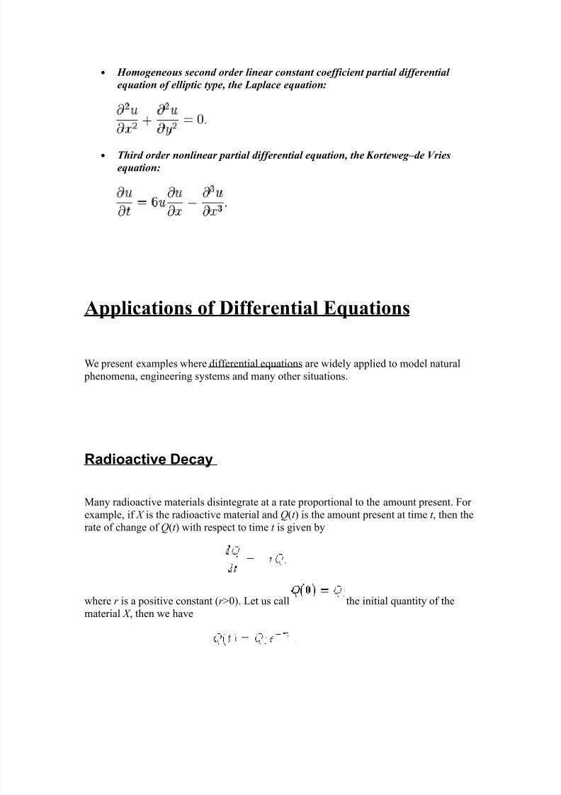
Applications of Differential Equations

We present examples where differential equations are widely applied to model natural

 phenomena, engineering systems and many other situations.

Radioactive Decay

Many radioactive materials disintegrate at a rate proportional to the amount present. For 

example, if  X is the radioactive material and Q(t ) is the amount present at time t , then the

rate of change of Q(t ) with respect to time t is given by

where r is a positive constant (r >0). Let us call the initial quantity of the

material X , then we have

8/8/2019 Maths 101 Term Paper

http://slidepdf.com/reader/full/maths-101-term-paper 8/26

Clearly, in order to determine Q(t ) we need to find the constant r . This can be done using

what is called the half-life T of the material X . The half-life is the time span needed to

disintegrate half of the material. So, we have . An easy calculation gives

. Therefore, if we know T , we can get r and vice-versa. Many chemistry text-

 books contain the half-life of some important radioactive materials. For example, the

half-life of Carbon-14 is . Therefore, the constant r associated with

Carbon-14 is . As a side note, Carbon-14 is an important tool in the

archeological research known as radiocarbon dating.

Example: A radioactive isotope has a half-life of 16 days. You wish to have 30 g at theend of 30 days. How much radioisotope should you start with?

Solution: Since the half-life is given in days we will measure time in days. Let Q(t ) be

the amount present at time t and the amount we are looking for (the initial amount).We know that

,

where r is a constant. We use the half-life T to determine r . Indeed, we have

Hence, since

,

we get

Newton's Law of Cooling

From experimental observations it is known that (up to a ``satisfactory'' approximation)

the surface temperature of an object changes at a rate proportional to its relative

temperature. That is, the difference between its temperature and the temperature of the

8/8/2019 Maths 101 Term Paper

http://slidepdf.com/reader/full/maths-101-term-paper 9/26

surrounding environment. This is what is known as Newton's law of cooling. Thus, if 

is the temperature of the object at time t , then we have

where S is the temperature of the surrounding environment. A qualitative study of this

 phenomena will show that k >0. This is a first order linear differential equation. The

solution, under the initial condition , is given by

Hence,

,

which implies

This equation makes it possible to find k if the interval of time is known and vice-

versa.

Example: Time of Death Suppose that a corpse was discovered in a motel room atmidnight and its temperature was . The temperature of the room is kept constant at

. Two hours later the temperature of the corpse dropped to . Find the time of 

death.

Solution: First we use the observed temperatures of the corpse to find the constant k . We

have

.

In order to find the time of death we need to remember that the temperature of a corpse at

time of death is (assuming the dead person was not sick!). Then we have

8/8/2019 Maths 101 Term Paper

http://slidepdf.com/reader/full/maths-101-term-paper 10/26

which means that the death happened around 7:26 P.M.

Orthogonal Trajectories

We have seen before that the solutions of a differential equation may be given by an

implicit equation with a parameter something like

This is an equation describing a family of curves. Whenever we fix the parameter C we

get one curve and vice-versa. For example, consider the families of curves

where m and C are parameters. Clearly, we may change the names of the variables and

still have the same geometric curves. For example, the above families define the samegeometric object as

 Note that the first family describes all the lines passing by the origin (0,0) while the

second the family describes all the circles centered at the origin (including the limit case

when the radius 0 which reduces to the single point (0,0)) (see the pictures below).

8/8/2019 Maths 101 Term Paper

http://slidepdf.com/reader/full/maths-101-term-paper 11/26

and

8/8/2019 Maths 101 Term Paper

http://slidepdf.com/reader/full/maths-101-term-paper 12/26

In this page, we will only use the variables x and y. Any family of curves will be written

as

One may ask whether any family of curves may be generated from a differential

equation? In general, the answer is no. Let us see how to proceed if the answer were to be

yes. First differentiate with respect to x, and get a new equation involving in general x, y,

, and C . Using the original equation, we may able to eliminate the parameter C from

the new equation.

Example. Find the differential equation satisfied by the family

8/8/2019 Maths 101 Term Paper

http://slidepdf.com/reader/full/maths-101-term-paper 13/26

Answer. We differentiate with respect to x, to get

Since we have

then we get

You may want to do some algebra to make the new equation easy to read. The next step isto rewrite this equation in the explicit form

this is the desired differential equation.

Example. Find the differential equation (in the explicit form) satisfied by the family

Answer. We have already found the differential equation in the implicit form

Algebraic manipulations give

Let us reconsider the example of the two families

If we draw the two families together on the same graph we get

8/8/2019 Maths 101 Term Paper

http://slidepdf.com/reader/full/maths-101-term-paper 14/26

As we see here something amazing happened. Indeed, it is clear that whenever one line

intersects one circle, the tangent line to the circle (at the point of intersection) and the line

are perpendicular or orthogonal. We say the two curves are orthogonal at the point of intersection.

Definition. Consider two families of curves and . We say that and are

orthogonal whenever any curve from intersects any curve from , the two curves are

orthogonal at the point of intersection.

For example, we have seen that the families y = m x and are orthogonal.

One may then ask the following natural question:

Given a family of curves , is it possible to find a family of curves which is

orthogonal to ? 

8/8/2019 Maths 101 Term Paper

http://slidepdf.com/reader/full/maths-101-term-paper 15/26

The answer to this question has many implications in many areas such as physics, fluid-

dynamics, etc... In general this question is very difficult. But in some cases, we may be

able to carry on the calculations and find the orthogonal family. Let us show how.

Consider the family of curves . We assume that an associated differential equation may

 be found, say

We know that for any curve from the family passing by the point ( x, y), the slope of the

tangent at this point is f ( x, y). Hence the slope of the line perpendicular (or orthogonal) to

this tangent is which happens to be the slope of the tangent line to theorthogonal curve passing by the point ( x, y). In other words, the family of orthogonal

curves are solutions to the differential equation

From this we see what we have to do. Indeed consider a family of curves . In order to

find the orthogonal family, we use the following practical steps

Step 1. Find the associated differential equation.

Step 2. Rewrite this differential equation in the explicit form

Step 3. Write down the differential equation associated to the orthogonal family

Step 4. Solve the new equation. The solutions are exactly the family of 

orthogonal curves.

Step 5. You may be asked to give a geometric view of the two families. Also you

may be asked to find a specific curve from the orthogonal family (something like

an IVP).

Example. Find the orthogonal family to the family of circles

8/8/2019 Maths 101 Term Paper

http://slidepdf.com/reader/full/maths-101-term-paper 16/26

Answer. First, we look for the differential equation satisfied by the circles. We

differentiate with respect to the variable x to get

We rewrite this equation in the explicit form

 Next we write down the equation for the orthogonal family

This is a linear as well as a separable equation. If we use the technique of linear 

equations, we get the integrating factor 

which gives

We recognize the family of lines and we confirm our earlier observation (that the two

families are indeed orthogonal).

This example is somehow easy and was given here to illustrate the technique.

Example. Find the orthogonal family to the family of circles

8/8/2019 Maths 101 Term Paper

http://slidepdf.com/reader/full/maths-101-term-paper 17/26

Answer. We have seen before that the explicit differential equation associated to the

family of circles is

Hence the differential equation for the orthogonal family is

We recognize an homogeneous equation. Let us use the technique developed to solve this

kind of equations. Consider the new variable (or equivalently y = x z ). Then wehave

8/8/2019 Maths 101 Term Paper

http://slidepdf.com/reader/full/maths-101-term-paper 18/26

and

Hence we have

Algebraic manipulations imply

This is a separable equation. The constant solutions are given by

which gives z =0. The non-constant solutions are found once we separate the variables

and then we integrate

Before we perform the integration for the left-hand side, we need to use partial

decomposition technique. We have

We will leave the details to you to show that A = 1, B=-2, and C =0. Hence we have

8/8/2019 Maths 101 Term Paper

http://slidepdf.com/reader/full/maths-101-term-paper 19/26

Hence

which is equivalent to

where . Putting all the solutions together we get

Going back to the variable y, we get

which is equivalent to

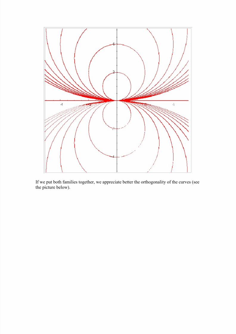
We recognize a family of circles centered on the y-axis and the line y=0 (the x-axis which

was easy to guess, isn't it?)

8/8/2019 Maths 101 Term Paper

http://slidepdf.com/reader/full/maths-101-term-paper 20/26

If we put both families together, we appreciate better the orthogonality of the curves (see

the picture below).

8/8/2019 Maths 101 Term Paper

http://slidepdf.com/reader/full/maths-101-term-paper 21/26

Population Dynamics

Here are some natural questions related to population problems:

• What will the population of a certain country be in ten years?

• How are we protecting the resources from extinction?

More can be said about the problem but, in this little review we will not discuss them in

detail. In order to illustrate the use of differential equations with regard to this problemwe consider the easiest mathematical model offered to govern the population dynamics of 

a certain species. It is commonly called the exponential model, that is, the rate of change

of the population is proportional to the existing population. In other words, if  P (t )

measures the population, we have

8/8/2019 Maths 101 Term Paper

http://slidepdf.com/reader/full/maths-101-term-paper 22/26

,

where the rate k is constant. It is fairly easy to see that if k > 0, we have growth, and if k <0, we have decay. This is a linear equation which solves into

,

where is the initial population, i.e. . Therefore, we conclude the following:

• if k >0, then the population grows and continues to expand to infinity, that is,

• if k <0, then the population will shrink and tend to 0. In other words we are facing

extinction.

Clearly, the first case, k >0, is not adequate and the model can be dropped. The main

argument for this has to do with environmental limitations. The complication is that

 population growth is eventually limited by some factor, usually one from among many

essential resources. When a population is far from its limits of growth it can growexponentially. However, when nearing its limits the population size can fluctuate, even

chaotically. Another model was proposed to remedy this flaw in the exponential model. It

is called the logistic model (also called Verhulst-Pearl model). The differential equationfor this model is

,

where M is a limiting size for the population (also called the carrying capacity). Clearly,

when P is small compared to M , the equation reduces to the exponential one. In order to

solve this equation we recognize a nonlinear equation which is separable. The constant

solutions are P =0 and P =M . The non-constant solutions may obtained by separating thevariables

,

and integration

8/8/2019 Maths 101 Term Paper

http://slidepdf.com/reader/full/maths-101-term-paper 23/26

The partial fraction techniques gives

,

which gives

Easy algebraic manipulations give

where C is a constant. Solving for  P , we get

If we consider the initial condition (assuming that is not equal to both 0 or M ), we get

,

which, once substituted into the expression for  P (t ) and simplified, we find

It is easy to see that

However, this is still not satisfactory because this model does not tell us when a population is facing extinction since it never implies that. Even starting with a small

 population it will always tend to the carrying capacity M .

8/8/2019 Maths 101 Term Paper

http://slidepdf.com/reader/full/maths-101-term-paper 24/26

Some other Applications to Engineering and

Sciences

Historically, it has been the needs of the physical sciences which have driven

the development of many parts of mathematics, particularly analysis. The

applications are sometimes difficult to classify mathematically, since tools

from several areas of mathematics may be applied. We focus on these

applications not by discussing the nature of their discipline but rather their 

interaction with mathematics.

• Mechanics of particles and systems studies dynamics of sets of 

 particles or solid bodies, including rotating and vibrating bodies. Uses

variational principles (energy-minimization) as well as differential

equations.

• Mechanics of deformable solids considers questions of elasticity and

 plasticity, wave propagation, engineering, and topics in specific solids

such as soils and crystals.

• Fluid mechanics studies air, water, and other fluids in motion:

compression, turbulence, diffusion, wave propagation, and so on.

Mathematically this includes study of solutions of differential

equations, including large-scale numerical methods (e.g the finite-

element method).• Optics, electromagnetic theory is the study of the propagation and

evolution of electromagnetic waves, including topics of interference

and diffraction. Besides the usual branches of analysis, this area

includes geometric topics such as the paths of light rays.

• Classical thermodynamics, heat transfer is the study of the flow of 

heat through matter, including phase change and combustion.

Historically, the source of Fourier series.

• Quantum Theory studies the solutions of the Schrödinger 

(differential) equation. Also includes a good deal of Lie group theory

and quantum group theory, theory of distributions and topics from

Functional analysis, Yang-Mills problems, Feynman diagrams, and so

on.

• Statistical mechanics, structure of matter is the study of large-scale

systems of particles, including stochastic systems and moving or 

8/8/2019 Maths 101 Term Paper

http://slidepdf.com/reader/full/maths-101-term-paper 25/26

evolving systems. Specific types of matter studied include fluids,

crystals, metals, and other solids.

• Relativity and gravitational theory is differential geometry,

analysis, and group theory applied to physics on a grand scale or in

extreme situations (e.g. black holes and cosmology).

• Astronomy and astrophysics: as celestial mechanics is,

mathematically, part of Mechanics of Particles (!), the principal

applications in this area appear to be concerning the structure,

evolution, and interaction of stars and galaxies.

• Geophysics applications typically involve material in Mechanics and

Fluid mechanics, as above, but for large-scale problems (this subject

deals with a very big solid and a large pool of fluid!)

• Systems theory; control study the evolution over time of complex

systems such as those in engineering. In particular, one may try to

identify the system -- to determine the equations or parameters whichgovern its development -- or to control the system -- to select the

 parameters (e.g. via feedback loops) to achieve a desired state. Of 

 particular interest are issues in stability (steady-state configurations)

and the effects of random changes and noise (stochastic systems).

While popularly the domain of "cybernetics" or "robotics", perhaps,

this is in practice a field of application of differential (or difference)

equations, functional analysis, numerical analysis, and global analysis

(or differential geometry).

•

Biology and other natural scienceswhose connections merit explicit

connection in the MSC scheme include Chemistry, Biology, Genetics,

and Medicine, In chemistry and biochemistry, it is clear that graph

theory, differential geometry, and differential equations play a role.

Medical technology uses techniques of information transfer and

visualization. Biology (including taxonomy and archaeobiology) use

statistical inference and other tools.

• Game theory, economics, social and behavioral sciences including

Psychology, Sociology, and other social sciences as a group. The more

 behavioural sciences (including Linguistics!) use a medley of 

statistical techniques, including experimental design and other rather combinatorial topics. Economics and finance also make use of 

statistical tools, especially time-series analysis; some topics, such as

voting theory, are more combinatorial. This category also includes

game theory, which is actually not about games at all but rather about

optimization; which combination of strategies leads to an optimal

outcome.

8/8/2019 Maths 101 Term Paper

http://slidepdf.com/reader/full/maths-101-term-paper 26/26

Observe that the branches of mathematics most closely allied with the fields

of mathematical physics are the parts of analysis, particularly those parts

related to differential equations. The other sciences draw on these as well as

 probability and statistics and, increasingly, numerical methods.