
Mathematical Programming Techniques in … Finding Efficient Solutions – Scalarization...
244
Introduction Finding Efficient Solutions – Scalarization Multiobjective Linear Programming Multiobjective Combinatorial Optimization Applications Commercials Mathematical Programming Techniques in Multiobjective Optimization Matthias Ehrgott Department of Engineering Science The University of Auckland, New Zealand Laboratoire d’Informatique de Nantes Atlantique CNRS, Nantes, France First IEEE Symposium on Computational Intelligence in Multi-Criteria Decision-Making, Honolulu, April 1 – 5 2007 Matthias Ehrgott Multiobjective Optimization
Transcript of Mathematical Programming Techniques in … Finding Efficient Solutions – Scalarization...

IntroductionFinding Efficient Solutions – Scalarization
Multiobjective Linear ProgrammingMultiobjective Combinatorial Optimization
ApplicationsCommercials
Mathematical Programming Techniques inMultiobjective Optimization
Matthias Ehrgott
Department of Engineering ScienceThe University of Auckland, New Zealand
Laboratoire d’Informatique de Nantes AtlantiqueCNRS, Nantes, France
First IEEE Symposium on Computational Intelligence inMulti-Criteria Decision-Making, Honolulu, April 1 – 5 2007
Matthias Ehrgott Multiobjective Optimization

IntroductionFinding Efficient Solutions – Scalarization
Multiobjective Linear ProgrammingMultiobjective Combinatorial Optimization
ApplicationsCommercials
1 IntroductionProblem Formulation and Definitions of Optimality
2 Finding Efficient Solutions – ScalarizationThe Idea of ScalarizationScalarization Techniques and Their Properties
3 Multiobjective Linear ProgrammingFormulation and the Fundamental TheoremSolving MOLPs in Decision and Objective Space
4 Multiobjective Combinatorial OptimizationDefinitions Revisited and CharacteristicsSolution Methods
5 Applications
6 Commercials
Matthias Ehrgott Multiobjective Optimization

IntroductionFinding Efficient Solutions – Scalarization
Multiobjective Linear ProgrammingMultiobjective Combinatorial Optimization
ApplicationsCommercials
Problem Formulation and Definitions of Optimality
Overview
1 IntroductionProblem Formulation and Definitions of Optimality
2 Finding Efficient Solutions – ScalarizationThe Idea of ScalarizationScalarization Techniques and Their Properties
3 Multiobjective Linear ProgrammingFormulation and the Fundamental TheoremSolving MOLPs in Decision and Objective Space
4 Multiobjective Combinatorial OptimizationDefinitions Revisited and CharacteristicsSolution Methods
5 Applications
6 Commercials
Matthias Ehrgott Multiobjective Optimization

IntroductionFinding Efficient Solutions – Scalarization
Multiobjective Linear ProgrammingMultiobjective Combinatorial Optimization
ApplicationsCommercials
Problem Formulation and Definitions of Optimality
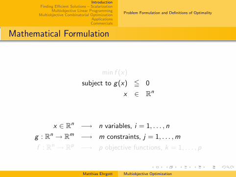
Mathematical Formulation
min f (x)
subject to g(x) 5 0
x ∈ Rn
x ∈ Rn −→ n variables, i = 1, . . . , n
g : Rn → Rm −→ m constraints, j = 1, . . . ,m
f : Rn → Rp −→ p objective functions, k = 1, . . . , p
Matthias Ehrgott Multiobjective Optimization
IntroductionFinding Efficient Solutions – Scalarization
Multiobjective Linear ProgrammingMultiobjective Combinatorial Optimization
ApplicationsCommercials
Problem Formulation and Definitions of Optimality
Mathematical Formulation
min f (x)
subject to g(x) 5 0
x ∈ Rn
x ∈ Rn −→ n variables, i = 1, . . . , n
g : Rn → Rm −→ m constraints, j = 1, . . . ,m
f : Rn → Rp −→ p objective functions, k = 1, . . . , p
Matthias Ehrgott Multiobjective Optimization

IntroductionFinding Efficient Solutions – Scalarization
Multiobjective Linear ProgrammingMultiobjective Combinatorial Optimization
ApplicationsCommercials
Problem Formulation and Definitions of Optimality
Feasible Sets
X = {x ∈ Rn : g(x) 5 0}feasible set in decision space
Y = f (X ) = {f (x) : x ∈ X}feasible set in objective space
0 1 2 3 4 5 6 7 8 9 100
1
2
3
4
5
6
7
8
9
10
Y = f(X)
Matthias Ehrgott Multiobjective Optimization
IntroductionFinding Efficient Solutions – Scalarization
Multiobjective Linear ProgrammingMultiobjective Combinatorial Optimization
ApplicationsCommercials
Problem Formulation and Definitions of Optimality
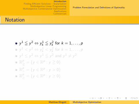
Notation
y1 5 y2 ⇔ y1k 5 y2
k for k = 1, . . . , p
y1 < y2 ⇔ y1k < y2
k for k = 1, . . . , p
y1 ≤ y2 ⇔ y1 5 y2 and y1 6= y2
Rp= = {y ∈ Rp : y = 0}
Rp> = {y ∈ Rp : y > 0}
Rp≥ = {y ∈ Rp : y ≥ 0}
Matthias Ehrgott Multiobjective Optimization

IntroductionFinding Efficient Solutions – Scalarization
Multiobjective Linear ProgrammingMultiobjective Combinatorial Optimization
ApplicationsCommercials
Problem Formulation and Definitions of Optimality
Notation
y1 5 y2 ⇔ y1k 5 y2
k for k = 1, . . . , p
y1 < y2 ⇔ y1k < y2
k for k = 1, . . . , p
y1 ≤ y2 ⇔ y1 5 y2 and y1 6= y2
Rp= = {y ∈ Rp : y = 0}
Rp> = {y ∈ Rp : y > 0}
Rp≥ = {y ∈ Rp : y ≥ 0}
Matthias Ehrgott Multiobjective Optimization
IntroductionFinding Efficient Solutions – Scalarization
Multiobjective Linear ProgrammingMultiobjective Combinatorial Optimization
ApplicationsCommercials
Problem Formulation and Definitions of Optimality
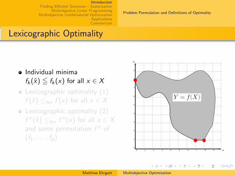
Lexicographic Optimality
Individual minimafk(x) 5 fk(x) for all x ∈ X
Lexicographic optimality (1)f (x) ≤lex f (x) for all x ∈ X
Lexicographic optimality (2)f π(x) ≤lex f π(x) for all x ∈ Xand some permutation f π of(f1, . . . , fp)
0 1 2 3 4 5 6 7 8 9 100
1
2
3
4
5
6
7
8
9
10
Y = f(X)
Matthias Ehrgott Multiobjective Optimization

IntroductionFinding Efficient Solutions – Scalarization
Multiobjective Linear ProgrammingMultiobjective Combinatorial Optimization
ApplicationsCommercials
Problem Formulation and Definitions of Optimality
(Weakly) Efficient Solutions
Weakly efficient solutions XwE
There is no x with f (x) < f (x)f (x) is weakly nondominatedYwN := f (XwN)
Efficient solutions XE
There is no x with f (x) ≤ f (x)f (x) is nondominatedYN := f (XE )
0 1 2 3 4 5 6 7 8 9 100
1
2
3
4
5
6
7
8
9
10
Y = f(X)
Matthias Ehrgott Multiobjective Optimization
IntroductionFinding Efficient Solutions – Scalarization
Multiobjective Linear ProgrammingMultiobjective Combinatorial Optimization
ApplicationsCommercials
Problem Formulation and Definitions of Optimality
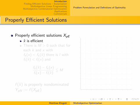
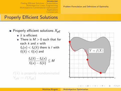
Properly Efficient Solutions
Properly efficient solutions XpE
x is efficientThere is M > 0 such that foreach k and x withfk(x) < fk(x) there is l withfl(x) < fl(x) and
fk(x)− fk(x)
fl(x)− fl(x)5 M
f (x) is properly nondominatedYpN := f (XpE ) 0 1 2 3 4 5 6 7 8 9 10
0
1
2
3
4
5
6
7
8
9
10
Matthias Ehrgott Multiobjective Optimization
IntroductionFinding Efficient Solutions – Scalarization
Multiobjective Linear ProgrammingMultiobjective Combinatorial Optimization
ApplicationsCommercials
Problem Formulation and Definitions of Optimality
Properly Efficient Solutions
Properly efficient solutions XpE
x is efficientThere is M > 0 such that foreach k and x withfk(x) < fk(x) there is l withfl(x) < fl(x) and
fk(x)− fk(x)
fl(x)− fl(x)5 M
f (x) is properly nondominatedYpN := f (XpE ) 0 1 2 3 4 5 6 7 8 9 10
0
1
2
3
4
5
6
7
8
9
10
Y = f(X)
Matthias Ehrgott Multiobjective Optimization
IntroductionFinding Efficient Solutions – Scalarization
Multiobjective Linear ProgrammingMultiobjective Combinatorial Optimization
ApplicationsCommercials
Problem Formulation and Definitions of Optimality
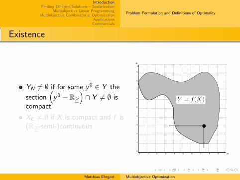
Existence
YN 6= ∅ if for some y0 ∈ Y the
section(y0 − R=
)∩ Y 6= ∅ is
compact
XE 6= ∅ if X is compact and f is(R=-semi-)continuous
0 1 2 3 4 5 6 7 8 9 100
1
2
3
4
5
6
7
8
9
10
Y = f(X)
Matthias Ehrgott Multiobjective Optimization

IntroductionFinding Efficient Solutions – Scalarization
Multiobjective Linear ProgrammingMultiobjective Combinatorial Optimization
ApplicationsCommercials
Problem Formulation and Definitions of Optimality
Existence
YN 6= ∅ if for some y0 ∈ Y the
section(y0 − R=
)∩ Y 6= ∅ is
compact
XE 6= ∅ if X is compact and f is(R=-semi-)continuous
0 1 2 3 4 5 6 7 8 9 100
1
2
3
4
5
6
7
8
9
10
Y = f(X)
Matthias Ehrgott Multiobjective Optimization
IntroductionFinding Efficient Solutions – Scalarization
Multiobjective Linear ProgrammingMultiobjective Combinatorial Optimization
ApplicationsCommercials
Problem Formulation and Definitions of Optimality
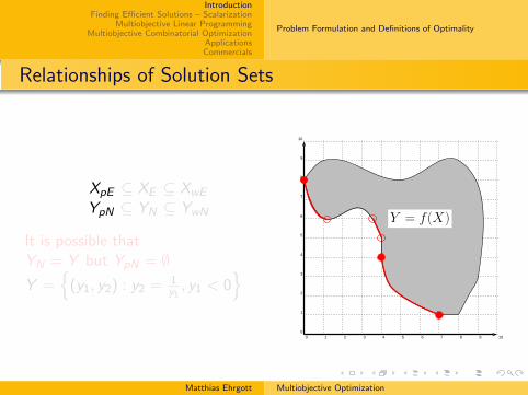
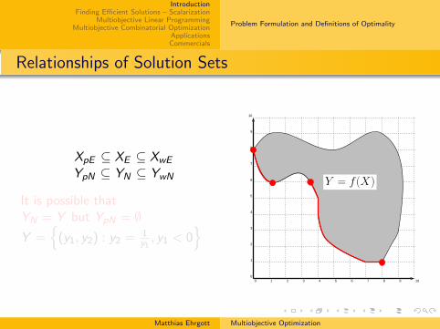
Relationships of Solution Sets
XpE ⊆ XE ⊆ XwE
YpN ⊆ YN ⊆ YwN
It is possible thatYN = Y but YpN = ∅Y =
{(y1, y2) : y2 = 1
y1, y1 < 0
}0 1 2 3 4 5 6 7 8 9 10
0
1
2
3
4
5
6
7
8
9
10
Y = f(X)
Matthias Ehrgott Multiobjective Optimization

IntroductionFinding Efficient Solutions – Scalarization
Multiobjective Linear ProgrammingMultiobjective Combinatorial Optimization
ApplicationsCommercials
Problem Formulation and Definitions of Optimality
Relationships of Solution Sets
XpE ⊆ XE ⊆ XwE
YpN ⊆ YN ⊆ YwN
It is possible thatYN = Y but YpN = ∅Y =
{(y1, y2) : y2 = 1
y1, y1 < 0
}0 1 2 3 4 5 6 7 8 9 10
0
1
2
3
4
5
6
7
8
9
10
Y = f(X)
Matthias Ehrgott Multiobjective Optimization

IntroductionFinding Efficient Solutions – Scalarization
Multiobjective Linear ProgrammingMultiobjective Combinatorial Optimization
ApplicationsCommercials
Problem Formulation and Definitions of Optimality
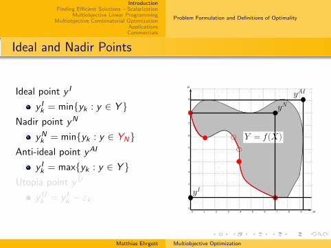
Ideal and Nadir Points
Ideal point y I
y Ik = min{yk : y ∈ Y }
Nadir point yN
yNk = min{yk : y ∈ YN}
Anti-ideal point yAI
y Ik = max{yk : y ∈ Y }
Utopia point yU
yUk = y I
k − εk
0 1 2 3 4 5 6 7 8 9 100
1
2
3
4
5
6
7
8
9
10
Y = f(X)
yI
Matthias Ehrgott Multiobjective Optimization

IntroductionFinding Efficient Solutions – Scalarization
Multiobjective Linear ProgrammingMultiobjective Combinatorial Optimization
ApplicationsCommercials
Problem Formulation and Definitions of Optimality
Ideal and Nadir Points
Ideal point y I
y Ik = min{yk : y ∈ Y }
Nadir point yN
yNk = min{yk : y ∈ YN}
Anti-ideal point yAI
y Ik = max{yk : y ∈ Y }
Utopia point yU
yUk = y I
k − εk
0 1 2 3 4 5 6 7 8 9 100
1
2
3
4
5
6
7
8
9
10
Y = f(X)
yI
yN
Matthias Ehrgott Multiobjective Optimization
IntroductionFinding Efficient Solutions – Scalarization
Multiobjective Linear ProgrammingMultiobjective Combinatorial Optimization
ApplicationsCommercials
Problem Formulation and Definitions of Optimality
Ideal and Nadir Points
Ideal point y I
y Ik = min{yk : y ∈ Y }
Nadir point yN
yNk = min{yk : y ∈ YN}
Anti-ideal point yAI
y Ik = max{yk : y ∈ Y }
Utopia point yU
yUk = y I
k − εk
0 1 2 3 4 5 6 7 8 9 100
1
2
3
4
5
6
7
8
9
10
Y = f(X)
yI
yN
yAI
Matthias Ehrgott Multiobjective Optimization

IntroductionFinding Efficient Solutions – Scalarization
Multiobjective Linear ProgrammingMultiobjective Combinatorial Optimization
ApplicationsCommercials
Problem Formulation and Definitions of Optimality
General Assumptions
XE is non-empty
y I 6= yN
0 1 2 3 4 5 6 7 8 9 100
1
2
3
4
5
6
7
8
9
10
Y = f(X)
yI
yN
Matthias Ehrgott Multiobjective Optimization

IntroductionFinding Efficient Solutions – Scalarization
Multiobjective Linear ProgrammingMultiobjective Combinatorial Optimization
ApplicationsCommercials
The Idea of ScalarizationScalarization Techniques and Their Properties
Overview
1 IntroductionProblem Formulation and Definitions of Optimality
2 Finding Efficient Solutions – ScalarizationThe Idea of ScalarizationScalarization Techniques and Their Properties
3 Multiobjective Linear ProgrammingFormulation and the Fundamental TheoremSolving MOLPs in Decision and Objective Space
4 Multiobjective Combinatorial OptimizationDefinitions Revisited and CharacteristicsSolution Methods
5 Applications
6 Commercials
Matthias Ehrgott Multiobjective Optimization
IntroductionFinding Efficient Solutions – Scalarization
Multiobjective Linear ProgrammingMultiobjective Combinatorial Optimization
ApplicationsCommercials
The Idea of ScalarizationScalarization Techniques and Their Properties
Principle of Scalarization
Convert multiobjective problem to (parameterized) single objectiveproblem and solve repeatedly with different parameter values
Desirable properties of scalarizations
Correctness: Optimal solutions are (weakly, properly) efficient
Completeness: All (weakly, properly) efficient solutions can befound
Matthias Ehrgott Multiobjective Optimization

IntroductionFinding Efficient Solutions – Scalarization
Multiobjective Linear ProgrammingMultiobjective Combinatorial Optimization
ApplicationsCommercials
The Idea of ScalarizationScalarization Techniques and Their Properties
Three Ideas for Scalarization
Aggregate objectives
Convert objectives to constraints
Minimize distance to ideal point
Matthias Ehrgott Multiobjective Optimization

IntroductionFinding Efficient Solutions – Scalarization
Multiobjective Linear ProgrammingMultiobjective Combinatorial Optimization
ApplicationsCommercials
The Idea of ScalarizationScalarization Techniques and Their Properties
Overview
1 IntroductionProblem Formulation and Definitions of Optimality
2 Finding Efficient Solutions – ScalarizationThe Idea of ScalarizationScalarization Techniques and Their Properties
3 Multiobjective Linear ProgrammingFormulation and the Fundamental TheoremSolving MOLPs in Decision and Objective Space
4 Multiobjective Combinatorial OptimizationDefinitions Revisited and CharacteristicsSolution Methods
5 Applications
6 Commercials
Matthias Ehrgott Multiobjective Optimization

IntroductionFinding Efficient Solutions – Scalarization
Multiobjective Linear ProgrammingMultiobjective Combinatorial Optimization
ApplicationsCommercials
The Idea of ScalarizationScalarization Techniques and Their Properties
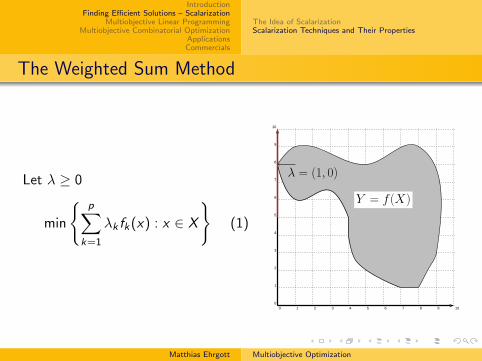
The Weighted Sum Method
Let λ ≥ 0
min
{p∑
k=1
λk fk(x) : x ∈ X
}(1)
0 1 2 3 4 5 6 7 8 9 100
1
2
3
4
5
6
7
8
9
10
Y = f(X)
λ = (0, 1)
Matthias Ehrgott Multiobjective Optimization

IntroductionFinding Efficient Solutions – Scalarization
Multiobjective Linear ProgrammingMultiobjective Combinatorial Optimization
ApplicationsCommercials
The Idea of ScalarizationScalarization Techniques and Their Properties
The Weighted Sum Method
Let λ ≥ 0
min
{p∑
k=1
λk fk(x) : x ∈ X
}(1)
0 1 2 3 4 5 6 7 8 9 100
1
2
3
4
5
6
7
8
9
10
Y = f(X)
λ = (1, 1)
Matthias Ehrgott Multiobjective Optimization
IntroductionFinding Efficient Solutions – Scalarization
Multiobjective Linear ProgrammingMultiobjective Combinatorial Optimization
ApplicationsCommercials
The Idea of ScalarizationScalarization Techniques and Their Properties
The Weighted Sum Method
Let λ ≥ 0
min
{p∑
k=1
λk fk(x) : x ∈ X
}(1)
0 1 2 3 4 5 6 7 8 9 100
1
2
3
4
5
6
7
8
9
10
Y = f(X)
λ = (1, 0)
Matthias Ehrgott Multiobjective Optimization

IntroductionFinding Efficient Solutions – Scalarization
Multiobjective Linear ProgrammingMultiobjective Combinatorial Optimization
ApplicationsCommercials
The Idea of ScalarizationScalarization Techniques and Their Properties
The Weighted Sum Method: Results
Theorem
Let x be an optimal solution of (1).
1 If λ ≥ 0 then x ∈ XwE .
2 If λ ≥ 0 and f (x) is unique then x ∈ XE .
3 If λ > 0 then x ∈ XpE .
Proof.
1 By contradiction
2 By contradiction
3 Construct M so that larger tradeoff would contradictoptimality of x
Matthias Ehrgott Multiobjective Optimization

IntroductionFinding Efficient Solutions – Scalarization
Multiobjective Linear ProgrammingMultiobjective Combinatorial Optimization
ApplicationsCommercials
The Idea of ScalarizationScalarization Techniques and Their Properties
The Weighted Sum Method: Results
Theorem (Geoffrion 1968)
Let X and f be such that Y = f (X ) is convex.
1 If x ∈ XwE then there is λ ≥ 0 such that x is an optimalsolution to (1).
2 If x ∈ XpE then there is λ > 0 such that x is an optimalsolution to (1).
Proof.
1 Apply separation theorem to (Y + Rp= − y) and −Rp
>
2 Apply separation theorem to (cl cone Y + Rp= − y) and −Rp
>
to show that weights are positive
3 If X and f are convex use properties of convex functionsMatthias Ehrgott Multiobjective Optimization

IntroductionFinding Efficient Solutions – Scalarization
Multiobjective Linear ProgrammingMultiobjective Combinatorial Optimization
ApplicationsCommercials
The Idea of ScalarizationScalarization Techniques and Their Properties
Nondominated and Properly Nondominated Points
....................................................................................................................................................................................................................................................................................................................
.......................
.
.
.
.
.
.
.
.
.
.
.
.
.
.
.
.
.
.
.
.
.
.
.
.
.
.
.
.
.
.
.
.
.
.
.
.
.
.
.
.
.
.
.
.
.
.
.
.
.
.
.
.
.
.
.
.
.
.
.
.
.
.
.
.
.
.
.
.
.
.
.
.
.
.
.
.
.
.
.
.
.
.
.
.
.
.
.
.
.
.
.
.
.
.
.
.
.
.
.
.
.
.
.
.
.
.
.
.
.
.
.
.
.
.
.
.
.
.
.
.
.
.
.
.
.
.
.
.
.
.
.
.
.
.
.
.
.
.
.
.
.
.
.
.
.
.
.
.
.
.
.
.
.
.
.
.
.
.
.
.
.
.
.
.
.
.
.
.
.
.
.
.
.
.
.
.
.
.
.
.
.
.
.
.
.
.
.
.
.
.
.
.
.
.
.
.
.
.
.
.
.
.
.
.
.
.
.
.
.
.
.
.
.
.
.
.
.
.
.
.
.
.
.
.
.
.
.
.
.
.
.
.
.
.
.
.
.
.
.
.
.
.
.
.
.
.
.
.
.
.
.
.
.
.
.
.
.
.
.
.
.
.
.
.
.
.
.
.
.
.
.
.
.
.
.
.
.
.
.
.
.
.
.
.
..
.
.
.
.
.
.
.
.
.
.
.
.
.
.
.
.
.
.
.
.
.
.
.
.
.
.
.
.
.
.
.
.
.
.
.
.
.
.
.
.
.
.
.
.
.
Y
YN ..........................................................................................................................................................................................................................................................................................................................................
.....................................................................................................................................................................................................................................................................................................................................................
•
•
••••••••••••••••••••••••••••••••••••••••••••••••••••••••••••••••••••••••••••••••••••••••••••••••••••••••••••••••••••••••••••••••••••••••••••••••••••••••••••••••••••••••
....................................................................................................................................................................................................................................................................................................................
.......................
.
.
.
.
.
.
.
.
.
.
.
.
.
.
.
.
.
.
.
.
.
.
.
.
.
.
.
.
.
.
.
.
.
.
.
.
.
.
.
.
.
.
.
.
.
.
.
.
.
.
.
.
.
.
.
.
.
.
.
.
.
.
.
.
.
.
.
.
.
.
.
.
.
.
.
.
.
.
.
.
.
.
.
.
.
.
.
.
.
.
.
.
.
.
.
.
.
.
.
.
.
.
.
.
.
.
.
.
.
.
.
.
.
.
.
.
.
.
.
.
.
.
.
.
.
.
.
.
.
.
.
.
.
.
.
.
.
.
.
.
.
.
.
.
.
.
.
.
.
.
.
.
.
.
.
.
.
.
.
.
.
.
.
.
.
.
.
.
.
.
.
.
.
.
.
.
.
.
.
.
.
.
.
.
.
.
.
.
.
.
.
.
.
.
.
.
.
.
.
.
.
.
.
.
.
.
.
.
.
.
.
.
.
.
.
.
.
.
.
.
.
.
.
.
.
.
.
.
.
.
.
.
.
.
.
.
.
.
.
.
.
.
.
.
.
.
.
.
.
.
.
.
.
.
.
.
.
.
.
.
.
.
.
.
.
.
.
.
.
.
.
.
.
.
.
.
.
.
.
.
.
.
.
.
..
.
.
.
.
.
.
.
.
.
.
.
.
.
.
.
.
.
.
.
.
.
.
.
.
.
.
.
.
.
.
.
.
.
.
.
.
.
.
.
.
.
.
.
.
.
Y
YpN............
..............................................................................................................................................................................................................................................................................................................................
.....................................................................................................................................................................................................................................................................................................................................................
◦
◦
•••••••••••••••••••••••••••••••••••••••••••••••••••••••••••••••••••••••••••••••••••••••••••••••••••••••••••••••••••••••••••••••••••••••••••••••••••••••••••••
XsE := {x ∈ X : x is optimal solution to (1) for some λ > 0}
Theorem
Assume that Y + Rp= is closed and convex. Then
YpN = f (XsE ) ⊆ YN ⊆ closure f (XsE ) = closure YpN
Matthias Ehrgott Multiobjective Optimization

IntroductionFinding Efficient Solutions – Scalarization
Multiobjective Linear ProgrammingMultiobjective Combinatorial Optimization
ApplicationsCommercials
The Idea of ScalarizationScalarization Techniques and Their Properties
Supported Efficient Solutions
Supported efficient solutions are efficient solutions with f (x) onthe convex hull of Y
0 1 2 3 4 5 6 7 8 9 100
1
2
3
4
5
6
7
8
9
10
conv(f(X)) + R2
≧
0 1 2 3 4 5 6 7 8 9 100
1
2
3
4
5
6
7
8
9
10
conv(f(X)) + R2
≧
Matthias Ehrgott Multiobjective Optimization

IntroductionFinding Efficient Solutions – Scalarization
Multiobjective Linear ProgrammingMultiobjective Combinatorial Optimization
ApplicationsCommercials
The Idea of ScalarizationScalarization Techniques and Their Properties
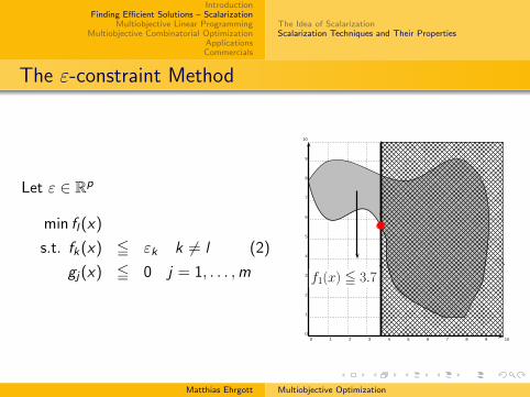
The ε-constraint Method
Let ε ∈ Rp
min fl(x)
s.t. fk(x) 5 εk k 6= l (2)
gj(x) 5 0 j = 1, . . . ,m
0 1 2 3 4 5 6 7 8 9 100
1
2
3
4
5
6
7
8
9
10
Y = f(X)
Matthias Ehrgott Multiobjective Optimization
IntroductionFinding Efficient Solutions – Scalarization
Multiobjective Linear ProgrammingMultiobjective Combinatorial Optimization
ApplicationsCommercials
The Idea of ScalarizationScalarization Techniques and Their Properties
The ε-constraint Method
Let ε ∈ Rp
min fl(x)
s.t. fk(x) 5 εk k 6= l (2)
gj(x) 5 0 j = 1, . . . ,m
0 1 2 3 4 5 6 7 8 9 100
1
2
3
4
5
6
7
8
9
10
f1(x) ≦ 3.7
Matthias Ehrgott Multiobjective Optimization

IntroductionFinding Efficient Solutions – Scalarization
Multiobjective Linear ProgrammingMultiobjective Combinatorial Optimization
ApplicationsCommercials
The Idea of ScalarizationScalarization Techniques and Their Properties
The ε-constraint Method
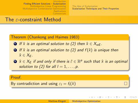
Theorem (Chankong and Haimes 1983)
1 If x is an optimal solution to (2) then x ∈ XwE .
2 If x is an optimal solution to (2) and f (x) is unique thenx ∈ XE .
3 x ∈ XE if and only if there is ε ∈ Rp such that x is an optimalsolution to (2) for all l = 1, . . . , p.
Proof.
By contradiction and using εl = fl(x)
Matthias Ehrgott Multiobjective Optimization

IntroductionFinding Efficient Solutions – Scalarization
Multiobjective Linear ProgrammingMultiobjective Combinatorial Optimization
ApplicationsCommercials
The Idea of ScalarizationScalarization Techniques and Their Properties
The ε-constraint Method
Theorem (Chankong and Haimes 1983)
1 If x is an optimal solution to (2) then x ∈ XwE .
2 If x is an optimal solution to (2) and f (x) is unique thenx ∈ XE .
3 x ∈ XE if and only if there is ε ∈ Rp such that x is an optimalsolution to (2) for all l = 1, . . . , p.
Proof.
By contradiction and using εl = fl(x)
Matthias Ehrgott Multiobjective Optimization
IntroductionFinding Efficient Solutions – Scalarization
Multiobjective Linear ProgrammingMultiobjective Combinatorial Optimization
ApplicationsCommercials
The Idea of ScalarizationScalarization Techniques and Their Properties
The Hybrid Method
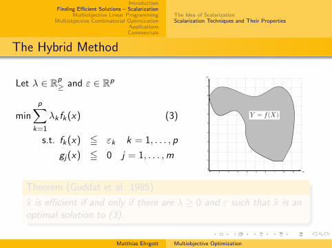
Let λ ∈ Rp≥ and ε ∈ Rp
min
p∑k=1
λk fk(x) (3)
s.t. fk(x) 5 εk k = 1, . . . , p
gj(x) 5 0 j = 1, . . . ,m
0 1 2 3 4 5 6 7 8 9 100
1
2
3
4
5
6
7
8
9
10
Y = f(X)
Theorem (Guddat et al. 1985)
x is efficient if and only if there are λ ≥ 0 and ε such that x is anoptimal solution to (3).
Matthias Ehrgott Multiobjective Optimization

IntroductionFinding Efficient Solutions – Scalarization
Multiobjective Linear ProgrammingMultiobjective Combinatorial Optimization
ApplicationsCommercials
The Idea of ScalarizationScalarization Techniques and Their Properties
The Hybrid Method
Let λ ∈ Rp≥ and ε ∈ Rp
min
p∑k=1
λk fk(x) (3)
s.t. fk(x) 5 εk k = 1, . . . , p
gj(x) 5 0 j = 1, . . . ,m
0 1 2 3 4 5 6 7 8 9 100
1
2
3
4
5
6
7
8
9
10
Theorem (Guddat et al. 1985)
x is efficient if and only if there are λ ≥ 0 and ε such that x is anoptimal solution to (3).
Matthias Ehrgott Multiobjective Optimization

IntroductionFinding Efficient Solutions – Scalarization
Multiobjective Linear ProgrammingMultiobjective Combinatorial Optimization
ApplicationsCommercials
The Idea of ScalarizationScalarization Techniques and Their Properties
Compromise Solutions
Let λ ∈ Rp≥ and 1 ≤ q < ∞
minx∈X
(p∑
k=1
λk(fk(x)− y Ik)q
) 1q
(4)
Let λ ∈ Rp≥
minx∈X
maxk=1,...,p
λk(fk(x)− y Ik) (5)
0 1 2 3 4 5 6 7 8 9 100
1
2
3
4
5
6
7
8
9
10
Y = f(X)
yI
Matthias Ehrgott Multiobjective Optimization

IntroductionFinding Efficient Solutions – Scalarization
Multiobjective Linear ProgrammingMultiobjective Combinatorial Optimization
ApplicationsCommercials
The Idea of ScalarizationScalarization Techniques and Their Properties
Compromise Solutions
Theorem
1 If x is a unique optimal solution to (4) or if λ > 0 then x isefficient.
2 If x is an optimal solution to (5) and λ > 0 then x is weaklyefficient.
3 If x is a unique optimal solution to (5) and λ > 0 then x isefficient.
Matthias Ehrgott Multiobjective Optimization
IntroductionFinding Efficient Solutions – Scalarization
Multiobjective Linear ProgrammingMultiobjective Combinatorial Optimization
ApplicationsCommercials
The Idea of ScalarizationScalarization Techniques and Their Properties
Compromise Solutions
For q = 1 (4) is the weighted sum scalarization
If y I is replaced by yU in (4) stronger results followSolutions obtained are properly efficient, and YN is containedin the closure of the set of all solutions obtained (Sawaragi etal. 1985)
True without convexity assumption, value of q indicates“degree of non-convexity”
Matthias Ehrgott Multiobjective Optimization
IntroductionFinding Efficient Solutions – Scalarization
Multiobjective Linear ProgrammingMultiobjective Combinatorial Optimization
ApplicationsCommercials
The Idea of ScalarizationScalarization Techniques and Their Properties
More General Concepts
lq norms can be replaced by more general distance functions
Ideal point can be replaced by a reference point and thedistance function by a ((strictly, strongly) increasing)achievement function Rp → R (Wierzbicki 1986)
min{sR(f (x)) : x ∈ X}sR(y) = maxk=1,...,p{λk(yk − yR
k )}+ ρ∑p
k=1(yk − yRk )
Matthias Ehrgott Multiobjective Optimization

IntroductionFinding Efficient Solutions – Scalarization
Multiobjective Linear ProgrammingMultiobjective Combinatorial Optimization
ApplicationsCommercials
Formulation and the Fundamental TheoremSolving MOLPs in Decision and Objective Space
Overview
1 IntroductionProblem Formulation and Definitions of Optimality
2 Finding Efficient Solutions – ScalarizationThe Idea of ScalarizationScalarization Techniques and Their Properties
3 Multiobjective Linear ProgrammingFormulation and the Fundamental TheoremSolving MOLPs in Decision and Objective Space
4 Multiobjective Combinatorial OptimizationDefinitions Revisited and CharacteristicsSolution Methods
5 Applications
6 Commercials
Matthias Ehrgott Multiobjective Optimization
IntroductionFinding Efficient Solutions – Scalarization
Multiobjective Linear ProgrammingMultiobjective Combinatorial Optimization
ApplicationsCommercials
Formulation and the Fundamental TheoremSolving MOLPs in Decision and Objective Space
MOLP Formulation
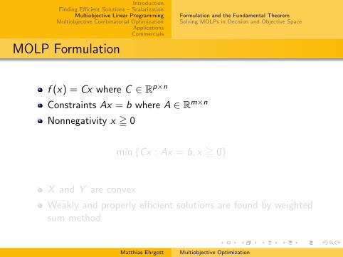
f (x) = Cx where C ∈ Rp×n
Constraints Ax = b where A ∈ Rm×n
Nonnegativity x = 0
min {Cx : Ax = b, x = 0}
X and Y are convex
Weakly and properly efficient solutions are found by weightedsum method
Matthias Ehrgott Multiobjective Optimization

IntroductionFinding Efficient Solutions – Scalarization
Multiobjective Linear ProgrammingMultiobjective Combinatorial Optimization
ApplicationsCommercials
Formulation and the Fundamental TheoremSolving MOLPs in Decision and Objective Space
MOLP Formulation
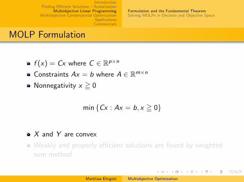
f (x) = Cx where C ∈ Rp×n
Constraints Ax = b where A ∈ Rm×n
Nonnegativity x = 0
min {Cx : Ax = b, x = 0}
X and Y are convex
Weakly and properly efficient solutions are found by weightedsum method
Matthias Ehrgott Multiobjective Optimization
IntroductionFinding Efficient Solutions – Scalarization
Multiobjective Linear ProgrammingMultiobjective Combinatorial Optimization
ApplicationsCommercials
Formulation and the Fundamental TheoremSolving MOLPs in Decision and Objective Space
MOLP Formulation
f (x) = Cx where C ∈ Rp×n
Constraints Ax = b where A ∈ Rm×n
Nonnegativity x = 0
min {Cx : Ax = b, x = 0}
X and Y are convex
Weakly and properly efficient solutions are found by weightedsum method
Matthias Ehrgott Multiobjective Optimization

IntroductionFinding Efficient Solutions – Scalarization
Multiobjective Linear ProgrammingMultiobjective Combinatorial Optimization
ApplicationsCommercials
Formulation and the Fundamental TheoremSolving MOLPs in Decision and Objective Space
MOLP Example
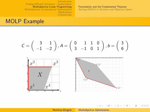
C =
(3 1
−1 −2
),A =
(0 1 1 03 −1 0 1
), b =
(36
)
0 1 2 3 40
1
2
3
4
X
x1
x2
x3
x4
0 1 2 3 4 5 6 7 8 9 10 11 12 13 140
-1
-2
-3
-4
-5
-6
-7
-8
-9
-10
Y
Cx1
Cx2
Cx3
Cx4
Matthias Ehrgott Multiobjective Optimization
IntroductionFinding Efficient Solutions – Scalarization
Multiobjective Linear ProgrammingMultiobjective Combinatorial Optimization
ApplicationsCommercials
Formulation and the Fundamental TheoremSolving MOLPs in Decision and Objective Space
MOLP Example
C =
(3 1
−1 −2
),A =
(0 1 1 03 −1 0 1
), b =
(36
)
0 1 2 3 40
1
2
3
4
X
x1
x2
x3
x4
0 1 2 3 4 5 6 7 8 9 10 11 12 13 140
-1
-2
-3
-4
-5
-6
-7
-8
-9
-10
Y
Cx1
Cx2
Cx3
Cx4
Matthias Ehrgott Multiobjective Optimization
IntroductionFinding Efficient Solutions – Scalarization
Multiobjective Linear ProgrammingMultiobjective Combinatorial Optimization
ApplicationsCommercials
Formulation and the Fundamental TheoremSolving MOLPs in Decision and Objective Space
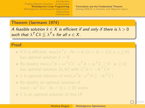
Theorem (Isermann 1974)
A feasible solution x ∈ X is efficient if and only if there is λ > 0such that λTCx 5 λT x for all x ∈ X.
Proof.
If x is efficient, max{eT z : Ax = b,Cx + Iz = Cx ; x , z = 0}has optimal solution z = 0
By duality min{uTb + wTCx : uTA = wTC = 0 : w = e}has optimal solution (u, w) with uTb = −wTCx
u is optimal solution of min{uTb : uTA = −wTC}By duality an optimal solution ofmax{−wTCx : Ax = b, x = 0} exists
x is an optimal solution of this LP
Matthias Ehrgott Multiobjective Optimization

IntroductionFinding Efficient Solutions – Scalarization
Multiobjective Linear ProgrammingMultiobjective Combinatorial Optimization
ApplicationsCommercials
Formulation and the Fundamental TheoremSolving MOLPs in Decision and Objective Space
Theorem (Isermann 1974)
A feasible solution x ∈ X is efficient if and only if there is λ > 0such that λTCx 5 λT x for all x ∈ X.
Proof.
If x is efficient, max{eT z : Ax = b,Cx + Iz = Cx ; x , z = 0}has optimal solution z = 0
By duality min{uTb + wTCx : uTA = wTC = 0 : w = e}has optimal solution (u, w) with uTb = −wTCx
u is optimal solution of min{uTb : uTA = −wTC}By duality an optimal solution ofmax{−wTCx : Ax = b, x = 0} exists
x is an optimal solution of this LP
Matthias Ehrgott Multiobjective Optimization
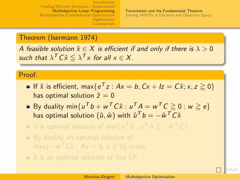
IntroductionFinding Efficient Solutions – Scalarization
Multiobjective Linear ProgrammingMultiobjective Combinatorial Optimization
ApplicationsCommercials
Formulation and the Fundamental TheoremSolving MOLPs in Decision and Objective Space
Overview
1 IntroductionProblem Formulation and Definitions of Optimality
2 Finding Efficient Solutions – ScalarizationThe Idea of ScalarizationScalarization Techniques and Their Properties
3 Multiobjective Linear ProgrammingFormulation and the Fundamental TheoremSolving MOLPs in Decision and Objective Space
4 Multiobjective Combinatorial OptimizationDefinitions Revisited and CharacteristicsSolution Methods
5 Applications
6 Commercials
Matthias Ehrgott Multiobjective Optimization
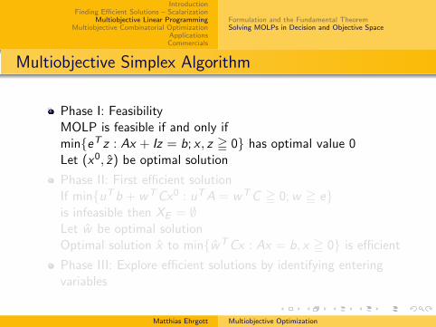
IntroductionFinding Efficient Solutions – Scalarization
Multiobjective Linear ProgrammingMultiobjective Combinatorial Optimization
ApplicationsCommercials
Formulation and the Fundamental TheoremSolving MOLPs in Decision and Objective Space
Multiobjective Simplex Algorithm
Phase I: FeasibilityMOLP is feasible if and only ifmin{eT z : Ax + Iz = b; x , z = 0} has optimal value 0Let (x0, z) be optimal solution
Phase II: First efficient solutionIf min{uTb + wTCx0 : uTA = wTC = 0;w = e}is infeasible then XE = ∅Let w be optimal solutionOptimal solution x to min{wTCx : Ax = b, x = 0} is efficient
Phase III: Explore efficient solutions by identifying enteringvariables
Matthias Ehrgott Multiobjective Optimization

IntroductionFinding Efficient Solutions – Scalarization
Multiobjective Linear ProgrammingMultiobjective Combinatorial Optimization
ApplicationsCommercials
Formulation and the Fundamental TheoremSolving MOLPs in Decision and Objective Space
Multiobjective Simplex Algorithm
Reduced cost matrix
R := (C − CBA−1B A)N
xj is efficient nonbasic variable if there is λ > 0 such thatλTR = 0 and λT r j = 0
At every efficient basis there exists an efficient nonbasicvariable and every feasible pivot leads to another efficient basis
Theorem (Evans and Steuer 1973)
Nonbasic variable xj is efficient if and only if the LP
max{eT v : Rz − r jδ + Iv = 0, zδ, v = 0}
has an optimal value of 0.
Matthias Ehrgott Multiobjective Optimization

IntroductionFinding Efficient Solutions – Scalarization
Multiobjective Linear ProgrammingMultiobjective Combinatorial Optimization
ApplicationsCommercials
Formulation and the Fundamental TheoremSolving MOLPs in Decision and Objective Space
Theorem
The set of all efficient bases is connected by pivots withefficient entering variables.
The set of all efficient extreme points of XE is connected byefficient edges.
The set of all nondominated extreme points of YN isconnected by nondominated edges.
Matthias Ehrgott Multiobjective Optimization

IntroductionFinding Efficient Solutions – Scalarization
Multiobjective Linear ProgrammingMultiobjective Combinatorial Optimization
ApplicationsCommercials
Formulation and the Fundamental TheoremSolving MOLPs in Decision and Objective Space
Phase I: MOLP is feasiblex0 = (0, 0)
Phase II: Optimal weightw = (1, 1)
Phase II: First efficient solutionx2 = (0, 3)
Phase III: Efficient enteringvariables s1, x2
Phase III: Efficient solutionsx1 = (0, 0), x3 = (3, 3)
Phase III: No more efficiententering variables
0 1 2 3 40
1
2
3
4
X
x1
x2
x3
x4
Matthias Ehrgott Multiobjective Optimization
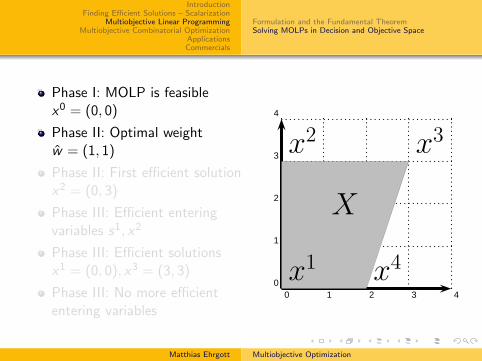
IntroductionFinding Efficient Solutions – Scalarization
Multiobjective Linear ProgrammingMultiobjective Combinatorial Optimization
ApplicationsCommercials
Formulation and the Fundamental TheoremSolving MOLPs in Decision and Objective Space
Phase I: MOLP is feasiblex0 = (0, 0)
Phase II: Optimal weightw = (1, 1)
Phase II: First efficient solutionx2 = (0, 3)
Phase III: Efficient enteringvariables s1, x2
Phase III: Efficient solutionsx1 = (0, 0), x3 = (3, 3)
Phase III: No more efficiententering variables
0 1 2 3 40
1
2
3
4
X
x1
x2
x3
x4
Matthias Ehrgott Multiobjective Optimization

IntroductionFinding Efficient Solutions – Scalarization
Multiobjective Linear ProgrammingMultiobjective Combinatorial Optimization
ApplicationsCommercials
Formulation and the Fundamental TheoremSolving MOLPs in Decision and Objective Space
Solving MOLPs in Objective Space
(Benson 1998)
Degeneracy causes problems for simplex algorithm
Decisions based on objective function values
Usually dim Y 5 p << dim X
Assume X is bounded
Theorem (Benson 1998)
The dimension of Y + Rp= is p and (Y + Rp
=)N = YN .
Y ′ := (Y + Rp=) ∩ (yAI − Rp
=)
Matthias Ehrgott Multiobjective Optimization
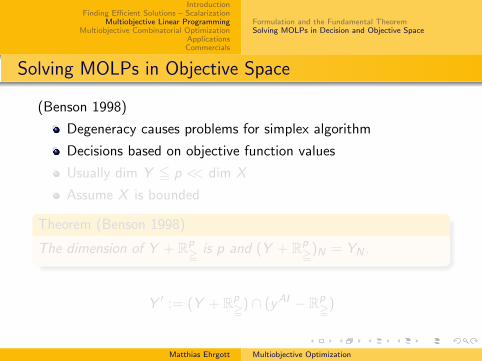
IntroductionFinding Efficient Solutions – Scalarization
Multiobjective Linear ProgrammingMultiobjective Combinatorial Optimization
ApplicationsCommercials
Formulation and the Fundamental TheoremSolving MOLPs in Decision and Objective Space
Solving MOLPs in Objective Space
(Benson 1998)
Degeneracy causes problems for simplex algorithm
Decisions based on objective function values
Usually dim Y 5 p << dim X
Assume X is bounded
Theorem (Benson 1998)
The dimension of Y + Rp= is p and (Y + Rp
=)N = YN .
Y ′ := (Y + Rp=) ∩ (yAI − Rp
=)
Matthias Ehrgott Multiobjective Optimization

IntroductionFinding Efficient Solutions – Scalarization
Multiobjective Linear ProgrammingMultiobjective Combinatorial Optimization
ApplicationsCommercials
Formulation and the Fundamental TheoremSolving MOLPs in Decision and Objective Space
Let p ∈ int Y ′
Let y be solution ofmin{eT y : y ∈ Y }Simplex S0 such that Y ′ ⊆ S0
defined by axes-parallelhyperplanes and supportinghyperplane with normal e at y
While Sk 6= Y ′
Find vertex yk of Sk−1 withsk /∈ Y ′
Find αk > 0 such thatαyk + (1− α)p is on theboundary of Y ′
Find supporting hyperplane toY ′ through boundary point
-6
-9
01263
Y
1y
2y
'Y
131
-4
S0
__
p
-16
-3-2
Vertices of S k
-6
-9
01263 1263
YY
1y
2y
'Y
131
-4
S0S0
__
p
-16
-3-2
-16
-3-2
Vertices of S kS k
Matthias Ehrgott Multiobjective Optimization

IntroductionFinding Efficient Solutions – Scalarization
Multiobjective Linear ProgrammingMultiobjective Combinatorial Optimization
ApplicationsCommercials
Formulation and the Fundamental TheoremSolving MOLPs in Decision and Objective Space
Let p ∈ int Y ′
Let y be solution ofmin{eT y : y ∈ Y }Simplex S0 such that Y ′ ⊆ S0
defined by axes-parallelhyperplanes and supportinghyperplane with normal e at y
While Sk 6= Y ′
Find vertex yk of Sk−1 withsk /∈ Y ′
Find αk > 0 such thatαyk + (1− α)p is on theboundary of Y ′
Find supporting hyperplane toY ′ through boundary point
-6
-9
01263
Y
1y
2y
'Y
131
-16
-4__
p
S1
-3-2
Vertex being cut out
Boundary point of on line segment
Vertices ofky
kq 'Y ),(__
pyk
S k
-6
-9
01263 1263
YY
1y
2y
'Y
131
-16
-4__
p
S1S1
-3-2
Vertex being cut out
Boundary point of on line segment
Vertices ofky
kq 'Y ),(__
pyk
S kS k
Matthias Ehrgott Multiobjective Optimization

IntroductionFinding Efficient Solutions – Scalarization
Multiobjective Linear ProgrammingMultiobjective Combinatorial Optimization
ApplicationsCommercials
Formulation and the Fundamental TheoremSolving MOLPs in Decision and Objective Space
Let p ∈ int Y ′
Let y be solution ofmin{eT y : y ∈ Y }Simplex S0 such that Y ′ ⊆ S0
defined by axes-parallelhyperplanes and supportinghyperplane with normal e at y
While Sk 6= Y ′
Find vertex yk of Sk−1 withsk /∈ Y ′
Find αk > 0 such thatαyk + (1− α)p is on theboundary of Y ′
Find supporting hyperplane toY ′ through boundary point
-6
-9
01263
Y
1y
2y
'Y
131
-16
-4__
p-3-2
S2
Vertex being cut out
Boundary point of on line segment
Vertices ofky
kq 'Y ),(__
pyk
S k
-6
-9
01263 1263
YY
1y
2y
'Y
131
-16
-4__
p-3-2
S2S2
Vertex being cut out
Boundary point of on line segment
Vertices ofky
kq 'Y ),(__
pyk
S kS k
Matthias Ehrgott Multiobjective Optimization

IntroductionFinding Efficient Solutions – Scalarization
Multiobjective Linear ProgrammingMultiobjective Combinatorial Optimization
ApplicationsCommercials
Formulation and the Fundamental TheoremSolving MOLPs in Decision and Objective Space
Let p ∈ int Y ′
Let y be solution ofmin{eT y : y ∈ Y }Simplex S0 such that Y ′ ⊆ S0
defined by axes-parallelhyperplanes and supportinghyperplane with normal e at y
While Sk 6= Y ′
Find vertex yk of Sk−1 withsk /∈ Y ′
Find αk > 0 such thatαyk + (1− α)p is on theboundary of Y ′
Find supporting hyperplane toY ′ through boundary point
-3-2
-6
-9
01263
Y
1y
2y
'Y
131
-4__
p
S3
-16
Vertex being cut out
Boundary point of on line segment
Vertices ofky
kq 'Y ),(__
pyk
S k
-3-2
-6
-9
01263 1263
YY
1y
2y
'Y
131
-4__
p
S3S3
-16
Vertex being cut out
Boundary point of on line segment
Vertices ofky
kq 'Y ),(__
pyk
S kS k
Matthias Ehrgott Multiobjective Optimization

IntroductionFinding Efficient Solutions – Scalarization
Multiobjective Linear ProgrammingMultiobjective Combinatorial Optimization
ApplicationsCommercials
Formulation and the Fundamental TheoremSolving MOLPs in Decision and Objective Space
Let p ∈ int Y ′
Let y be solution ofmin{eT y : y ∈ Y }Simplex S0 such that Y ′ ⊆ S0
defined by axes-parallelhyperplanes and supportinghyperplane with normal e at y
While Sk 6= Y ′
Find vertex yk of Sk−1 withsk /∈ Y ′
Find αk > 0 such thatαyk + (1− α)p is on theboundary of Y ′
Find supporting hyperplane toY ′ through boundary point
-3-2
-6
-9
01263
Y
1y
2y
'Y
131
-4__
p
S4
-16
Vertex being cut out
Boundary point of on line segment
Vertices ofky
kq 'Y ),(__
pyk
S k
-3-2
-6
-9
01263 1263
YY
1y
2y
'Y
131
-4__
p
S4S4
-16
Vertex being cut out
Boundary point of on line segment
Vertices ofky
kq 'Y ),(__
pyk
S kS k
Matthias Ehrgott Multiobjective Optimization

IntroductionFinding Efficient Solutions – Scalarization
Multiobjective Linear ProgrammingMultiobjective Combinatorial Optimization
ApplicationsCommercials
Definitions Revisited and CharacteristicsSolution Methods
Overview
1 IntroductionProblem Formulation and Definitions of Optimality
2 Finding Efficient Solutions – ScalarizationThe Idea of ScalarizationScalarization Techniques and Their Properties
3 Multiobjective Linear ProgrammingFormulation and the Fundamental TheoremSolving MOLPs in Decision and Objective Space
4 Multiobjective Combinatorial OptimizationDefinitions Revisited and CharacteristicsSolution Methods
5 Applications
6 Commercials
Matthias Ehrgott Multiobjective Optimization

IntroductionFinding Efficient Solutions – Scalarization
Multiobjective Linear ProgrammingMultiobjective Combinatorial Optimization
ApplicationsCommercials
Definitions Revisited and CharacteristicsSolution Methods
Mathematical Formulation
min z(x) = Cx
subject to Ax = b
x ∈ {0, 1}n
x ∈ {0, 1}n −→ n variables, i = 1, . . . , n
C ∈ Zp×n −→ p objective functions, k = 1, . . . , p
A ∈ Zm×n −→ m constraints, j = 1, . . . ,m
Matthias Ehrgott Multiobjective Optimization

IntroductionFinding Efficient Solutions – Scalarization
Multiobjective Linear ProgrammingMultiobjective Combinatorial Optimization
ApplicationsCommercials
Definitions Revisited and CharacteristicsSolution Methods
Feasible Sets
X = {x ∈ {0, 1}n : Ax = b}feasible set in decision space
Y = z(X ) = {Cx : x ∈ X}feasible set in objective space
conv(Y ) + Rp=
0 1 2 3 4 5 6 7 8 9 100
1
2
3
4
5
6
7
8
9
10
Y = C(X)
Matthias Ehrgott Multiobjective Optimization

IntroductionFinding Efficient Solutions – Scalarization
Multiobjective Linear ProgrammingMultiobjective Combinatorial Optimization
ApplicationsCommercials
Definitions Revisited and CharacteristicsSolution Methods
Feasible Sets
X = {x ∈ {0, 1}n : Ax = b}feasible set in decision space
Y = z(X ) = {Cx : x ∈ X}feasible set in objective space
conv(Y ) + Rp=
0 1 2 3 4 5 6 7 8 9 100
1
2
3
4
5
6
7
8
9
10
conv(C(X)) + Rp
≧
Matthias Ehrgott Multiobjective Optimization

IntroductionFinding Efficient Solutions – Scalarization
Multiobjective Linear ProgrammingMultiobjective Combinatorial Optimization
ApplicationsCommercials
Definitions Revisited and CharacteristicsSolution Methods
Lexicographic Optimality
Individual minimazk(x) 5 zk(x) for all x ∈ X
Lexicographic optimality (1)z(x) ≤lex z(x) for all x ∈ X
Lexicographic optimality (2)zπ(x) ≤lex zπ(x) for all x ∈ Xand some permutation zπ of(z1, . . . , zp)
0 1 2 3 4 5 6 7 8 9 100
1
2
3
4
5
6
7
8
9
10
Matthias Ehrgott Multiobjective Optimization
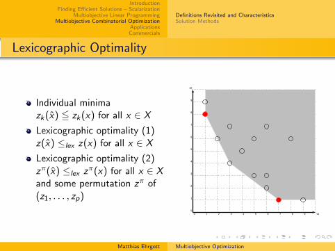
IntroductionFinding Efficient Solutions – Scalarization
Multiobjective Linear ProgrammingMultiobjective Combinatorial Optimization
ApplicationsCommercials
Definitions Revisited and CharacteristicsSolution Methods
Lexicographic Optimality
Individual minimazk(x) 5 zk(x) for all x ∈ X
Lexicographic optimality (1)z(x) ≤lex z(x) for all x ∈ X
Lexicographic optimality (2)zπ(x) ≤lex zπ(x) for all x ∈ Xand some permutation zπ of(z1, . . . , zp)
0 1 2 3 4 5 6 7 8 9 100
1
2
3
4
5
6
7
8
9
10
Matthias Ehrgott Multiobjective Optimization

IntroductionFinding Efficient Solutions – Scalarization
Multiobjective Linear ProgrammingMultiobjective Combinatorial Optimization
ApplicationsCommercials
Definitions Revisited and CharacteristicsSolution Methods
Efficient Solutions
Weakly efficient solutions XwE
There is no x with z(x) < z(x)z(x) is weakly nondominatedYwN := z(XwN)
Efficient solutions XE
There is no x with z(x) ≤ z(x)z(x) is nondominatedYN := z(XE )
0 1 2 3 4 5 6 7 8 9 100
1
2
3
4
5
6
7
8
9
10
Matthias Ehrgott Multiobjective Optimization
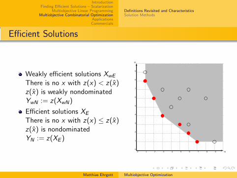
IntroductionFinding Efficient Solutions – Scalarization
Multiobjective Linear ProgrammingMultiobjective Combinatorial Optimization
ApplicationsCommercials
Definitions Revisited and CharacteristicsSolution Methods
Efficient Solutions
Weakly efficient solutions XwE
There is no x with z(x) < z(x)z(x) is weakly nondominatedYwN := z(XwN)
Efficient solutions XE
There is no x with z(x) ≤ z(x)z(x) is nondominatedYN := z(XE )
0 1 2 3 4 5 6 7 8 9 100
1
2
3
4
5
6
7
8
9
10
Matthias Ehrgott Multiobjective Optimization

IntroductionFinding Efficient Solutions – Scalarization
Multiobjective Linear ProgrammingMultiobjective Combinatorial Optimization
ApplicationsCommercials
Definitions Revisited and CharacteristicsSolution Methods
Efficient Solutions
Supported efficient solutionsXsE : There is λ > 0 withλTCx 5 λTCx for all x ∈ X
Cx is extreme point ofconv(Y ) + Rp
= → XsE1
Cx is in relative interior offace of conv(Y ) + Rp
= → XsE2
Nonsupported efficient solutionsXnE : Cx is in interior ofconv(Y ) + Rp
=0 1 2 3 4 5 6 7 8 9 10
0
1
2
3
4
5
6
7
8
9
10
conv(C(X)) + Rp
≧
λ =(
5
6, 1
6
)
Matthias Ehrgott Multiobjective Optimization

IntroductionFinding Efficient Solutions – Scalarization
Multiobjective Linear ProgrammingMultiobjective Combinatorial Optimization
ApplicationsCommercials
Definitions Revisited and CharacteristicsSolution Methods
Efficient Solutions
Supported efficient solutionsXsE : There is λ > 0 withλTCx 5 λTCx for all x ∈ X
Cx is extreme point ofconv(Y ) + Rp
= → XsE1
Cx is in relative interior offace of conv(Y ) + Rp
= → XsE2
Nonsupported efficient solutionsXnE : Cx is in interior ofconv(Y ) + Rp
=0 1 2 3 4 5 6 7 8 9 10
0
1
2
3
4
5
6
7
8
9
10
conv(C(X)) + Rp
≧
λ =(
1
2, 1
2
)
Matthias Ehrgott Multiobjective Optimization
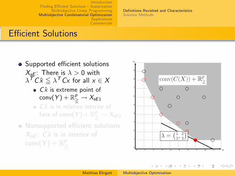
IntroductionFinding Efficient Solutions – Scalarization
Multiobjective Linear ProgrammingMultiobjective Combinatorial Optimization
ApplicationsCommercials
Definitions Revisited and CharacteristicsSolution Methods
Efficient Solutions
Supported efficient solutionsXsE : There is λ > 0 withλTCx 5 λTCx for all x ∈ X
Cx is extreme point ofconv(Y ) + Rp
= → XsE1
Cx is in relative interior offace of conv(Y ) + Rp
= → XsE2
Nonsupported efficient solutionsXnE : Cx is in interior ofconv(Y ) + Rp
=0 1 2 3 4 5 6 7 8 9 10
0
1
2
3
4
5
6
7
8
9
10
conv(C(X)) + Rp
≧
λ =(
1
3, 2
3
)
Matthias Ehrgott Multiobjective Optimization

IntroductionFinding Efficient Solutions – Scalarization
Multiobjective Linear ProgrammingMultiobjective Combinatorial Optimization
ApplicationsCommercials
Definitions Revisited and CharacteristicsSolution Methods
Efficient Solutions
Supported efficient solutionsXsE : There is λ > 0 withλTCx 5 λTCx for all x ∈ X
Cx is extreme point ofconv(Y ) + Rp
= → XsE1
Cx is in relative interior offace of conv(Y ) + Rp
= → XsE2
Nonsupported efficient solutionsXnE : Cx is in interior ofconv(Y ) + Rp
=0 1 2 3 4 5 6 7 8 9 10
0
1
2
3
4
5
6
7
8
9
10
conv(C(X)) + Rp
≧
λ =(
2
3, 1
3
)
Matthias Ehrgott Multiobjective Optimization

IntroductionFinding Efficient Solutions – Scalarization
Multiobjective Linear ProgrammingMultiobjective Combinatorial Optimization
ApplicationsCommercials
Definitions Revisited and CharacteristicsSolution Methods
Efficient Solutions
Supported efficient solutionsXsE : There is λ > 0 withλTCx 5 λTCx for all x ∈ X
Cx is extreme point ofconv(Y ) + Rp
= → XsE1
Cx is in relative interior offace of conv(Y ) + Rp
= → XsE2
Nonsupported efficient solutionsXnE : Cx is in interior ofconv(Y ) + Rp
=
0 1 2 3 4 5 6 7 8 9 100
1
2
3
4
5
6
7
8
9
10
conv(C(X)) + Rp
≧
Matthias Ehrgott Multiobjective Optimization
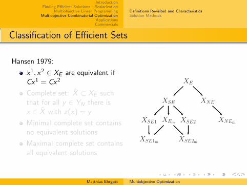
IntroductionFinding Efficient Solutions – Scalarization
Multiobjective Linear ProgrammingMultiobjective Combinatorial Optimization
ApplicationsCommercials
Definitions Revisited and CharacteristicsSolution Methods
Classification of Efficient Sets
Hansen 1979:
x1, x2 ∈ XE are equivalent ifCx1 = Cx2
Complete set: X ⊂ XE suchthat for all y ∈ YN there isx ∈ X with z(x) = y
Minimal complete set containsno equivalent solutions
Maximal complete set containsall equivalent solutions
XE
XSE XNE
XSE1 XEm XSE2 XNEm
XSE1mXSE2m
Matthias Ehrgott Multiobjective Optimization

IntroductionFinding Efficient Solutions – Scalarization
Multiobjective Linear ProgrammingMultiobjective Combinatorial Optimization
ApplicationsCommercials
Definitions Revisited and CharacteristicsSolution Methods
MOCO Problems Are Hard
Theorem
Multiobjective combinatorial optimization problems are NP-hard,#P-complete, and intractable.
Examples:
Shortest path (Hansen 1979, Serafini 1986)
Assignment (Serafini 1986, Neumayer 1994)
Spanning tree (Hamacher and Ruhe 1994)
Network flow (Ruhe 1988)
Matthias Ehrgott Multiobjective Optimization

IntroductionFinding Efficient Solutions – Scalarization
Multiobjective Linear ProgrammingMultiobjective Combinatorial Optimization
ApplicationsCommercials
Definitions Revisited and CharacteristicsSolution Methods
Number of Efficient Solutions
Intractable: XE , even YsN , can be exponential in the size of theinstance
Empirically often
|XnE | grows exponentially with instance size
|XsE | grows polynomially with instance size
But this depends on numerical values of C
Matthias Ehrgott Multiobjective Optimization
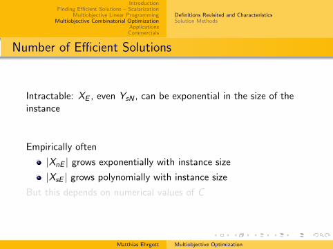
IntroductionFinding Efficient Solutions – Scalarization
Multiobjective Linear ProgrammingMultiobjective Combinatorial Optimization
ApplicationsCommercials
Definitions Revisited and CharacteristicsSolution Methods
Number of Efficient Solutions
Intractable: XE , even YsN , can be exponential in the size of theinstance
Empirically often
|XnE | grows exponentially with instance size
|XsE | grows polynomially with instance size
But this depends on numerical values of C
Matthias Ehrgott Multiobjective Optimization

IntroductionFinding Efficient Solutions – Scalarization
Multiobjective Linear ProgrammingMultiobjective Combinatorial Optimization
ApplicationsCommercials
Definitions Revisited and CharacteristicsSolution Methods
0
0.05
0.1
0.15
0.2
0.25
0.3
50 100 150 200 250 300 350 400 450 500
nb S
E p
ar r
ap. N
E
instance
Bi-KP Problems : proportion de supportees
ABCD
Matthias Ehrgott Multiobjective Optimization
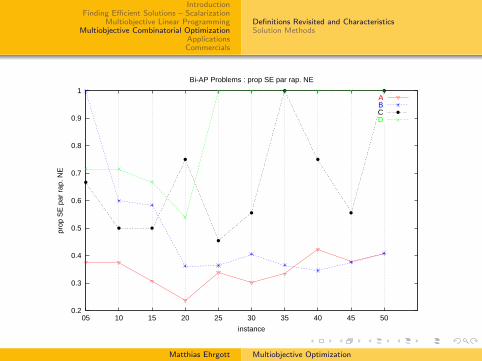
IntroductionFinding Efficient Solutions – Scalarization
Multiobjective Linear ProgrammingMultiobjective Combinatorial Optimization
ApplicationsCommercials
Definitions Revisited and CharacteristicsSolution Methods
0.2
0.3
0.4
0.5
0.6
0.7
0.8
0.9
1
05 10 15 20 25 30 35 40 45 50
prop
SE
par
rap
. NE
instance
Bi-AP Problems : prop SE par rap. NE
ABCD
Matthias Ehrgott Multiobjective Optimization

IntroductionFinding Efficient Solutions – Scalarization
Multiobjective Linear ProgrammingMultiobjective Combinatorial Optimization
ApplicationsCommercials
Definitions Revisited and CharacteristicsSolution Methods
Overview
1 IntroductionProblem Formulation and Definitions of Optimality
2 Finding Efficient Solutions – ScalarizationThe Idea of ScalarizationScalarization Techniques and Their Properties
3 Multiobjective Linear ProgrammingFormulation and the Fundamental TheoremSolving MOLPs in Decision and Objective Space
4 Multiobjective Combinatorial OptimizationDefinitions Revisited and CharacteristicsSolution Methods
5 Applications
6 Commercials
Matthias Ehrgott Multiobjective Optimization

IntroductionFinding Efficient Solutions – Scalarization
Multiobjective Linear ProgrammingMultiobjective Combinatorial Optimization
ApplicationsCommercials
Definitions Revisited and CharacteristicsSolution Methods
Solving MOCO Problems
Scalarization
Single objective problem polynomially solvable and algorithmcan be directly extended to multiple objectives
Single objective problem polynomially solvable and rankingalgorithm exists: The 2 Phase Method
Single objective problem NP-hard: General integerprogramming methods
Matthias Ehrgott Multiobjective Optimization

IntroductionFinding Efficient Solutions – Scalarization
Multiobjective Linear ProgrammingMultiobjective Combinatorial Optimization
ApplicationsCommercials
Definitions Revisited and CharacteristicsSolution Methods
Principle and Properties of Scalarization
Convert multiobjective problem to (parameterized) single objectiveproblem and solve repeatedly with different parameter values
Desirable properties of scalarizations: (Wierzbicki 1984)
Correctness: Optimal solutions are (weakly) efficient
Completeness: All efficient solutions can be found
Computability: Scalarization is not harder than singleobjective version of problem (theory and practice)
Linearity: Scalarization has linear formulation
Matthias Ehrgott Multiobjective Optimization
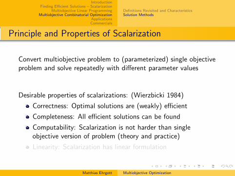
IntroductionFinding Efficient Solutions – Scalarization
Multiobjective Linear ProgrammingMultiobjective Combinatorial Optimization
ApplicationsCommercials
Definitions Revisited and CharacteristicsSolution Methods
Principle and Properties of Scalarization
Convert multiobjective problem to (parameterized) single objectiveproblem and solve repeatedly with different parameter values
Desirable properties of scalarizations: (Wierzbicki 1984)
Correctness: Optimal solutions are (weakly) efficient
Completeness: All efficient solutions can be found
Computability: Scalarization is not harder than singleobjective version of problem (theory and practice)
Linearity: Scalarization has linear formulation
Matthias Ehrgott Multiobjective Optimization

IntroductionFinding Efficient Solutions – Scalarization
Multiobjective Linear ProgrammingMultiobjective Combinatorial Optimization
ApplicationsCommercials
Definitions Revisited and CharacteristicsSolution Methods
Scalarization Methods
Weighted sum:
minx∈X
{λT z(x)
}ε-constraint:minx∈X
{zl(x) : zk(x) ≤ εk , k 6= l}
Weighted Chebychev:
minx∈X
{max
k=1,...,pνk(zk(x)− y I
k)
}0 1 2 3 4 5 6 7 8 9 10
0
1
2
3
4
5
6
7
8
9
10
λT=
(
3
7, 4
7
)
Matthias Ehrgott Multiobjective Optimization

IntroductionFinding Efficient Solutions – Scalarization
Multiobjective Linear ProgrammingMultiobjective Combinatorial Optimization
ApplicationsCommercials
Definitions Revisited and CharacteristicsSolution Methods
Scalarization Methods
Weighted sum:
minx∈X
{λT z(x)
}ε-constraint:minx∈X
{zl(x) : zk(x) ≤ εk , k 6= l}
Weighted Chebychev:
minx∈X
{max
k=1,...,pνk(zk(x)− y I
k)
}0 1 2 3 4 5 6 7 8 9 10
0
1
2
3
4
5
6
7
8
9
10
z1(x) ≤ 5.5
Matthias Ehrgott Multiobjective Optimization

IntroductionFinding Efficient Solutions – Scalarization
Multiobjective Linear ProgrammingMultiobjective Combinatorial Optimization
ApplicationsCommercials
Definitions Revisited and CharacteristicsSolution Methods
Scalarization Methods
Weighted sum:
minx∈X
{λT z(x)
}ε-constraint:minx∈X
{zl(x) : zk(x) ≤ εk , k 6= l}
Weighted Chebychev:
minx∈X
{max
k=1,...,pνk(zk(x)− y I
k)
}0 1 2 3 4 5 6 7 8 9 10
0
1
2
3
4
5
6
7
8
9
10
yI
ν2 = 1
ν1 = 0.5
Matthias Ehrgott Multiobjective Optimization
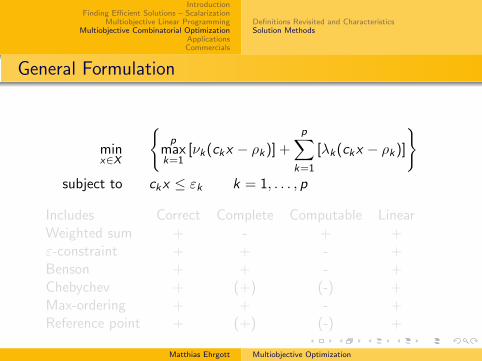
IntroductionFinding Efficient Solutions – Scalarization
Multiobjective Linear ProgrammingMultiobjective Combinatorial Optimization
ApplicationsCommercials
Definitions Revisited and CharacteristicsSolution Methods
General Formulation
minx∈X
{p
maxk=1
[νk(ckx − ρk)] +
p∑k=1
[λk(ckx − ρk)]
}subject to ckx ≤ εk k = 1, . . . , p
Includes Correct Complete Computable LinearWeighted sum + - + +ε-constraint + + - +Benson + + - +Chebychev + (+) (-) +Max-ordering + + - +Reference point + (+) (-) +
Matthias Ehrgott Multiobjective Optimization
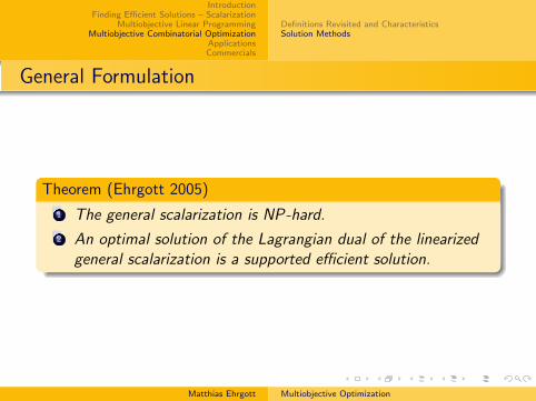
IntroductionFinding Efficient Solutions – Scalarization
Multiobjective Linear ProgrammingMultiobjective Combinatorial Optimization
ApplicationsCommercials
Definitions Revisited and CharacteristicsSolution Methods
General Formulation
Theorem (Ehrgott 2005)
1 The general scalarization is NP-hard.
2 An optimal solution of the Lagrangian dual of the linearizedgeneral scalarization is a supported efficient solution.
Matthias Ehrgott Multiobjective Optimization

IntroductionFinding Efficient Solutions – Scalarization
Multiobjective Linear ProgrammingMultiobjective Combinatorial Optimization
ApplicationsCommercials
Definitions Revisited and CharacteristicsSolution Methods
Method of Elastic Constraints
minx∈X
clx +∑k 6=l
µkwk
s.t. ckx + vk − wk ≤ εk k 6= l
vk ,wk ≥ 0 k 6= l
0 1 2 3 4 5 6 7 8 9 100
1
2
3
4
5
6
7
8
9
10
z1(x) ≤ 5.5
Matthias Ehrgott Multiobjective Optimization
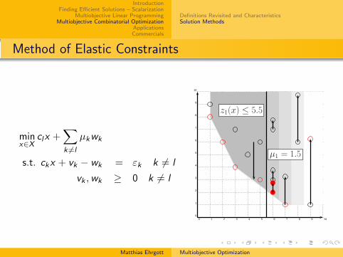
IntroductionFinding Efficient Solutions – Scalarization
Multiobjective Linear ProgrammingMultiobjective Combinatorial Optimization
ApplicationsCommercials
Definitions Revisited and CharacteristicsSolution Methods
Method of Elastic Constraints
minx∈X
clx +∑k 6=l
µkwk
s.t. ckx + vk − wk = εk k 6= l
vk ,wk ≥ 0 k 6= l
0 1 2 3 4 5 6 7 8 9 100
1
2
3
4
5
6
7
8
9
10
µ1 = 1.5
z1(x) ≤ 5.5
Matthias Ehrgott Multiobjective Optimization
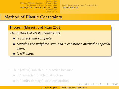
IntroductionFinding Efficient Solutions – Scalarization
Multiobjective Linear ProgrammingMultiobjective Combinatorial Optimization
ApplicationsCommercials
Definitions Revisited and CharacteristicsSolution Methods
Method of Elastic Constraints
Theorem (Ehrgott and Ryan 2002)
The method of elastic constraints
is correct and complete,
contains the weighted sum and ε-constraint method as specialcases,
is NP-hard.
... but (often) solvable in practice because
it “respects” problem structure
it “limits damage” of ε-constraints
Matthias Ehrgott Multiobjective Optimization
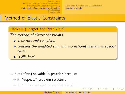
IntroductionFinding Efficient Solutions – Scalarization
Multiobjective Linear ProgrammingMultiobjective Combinatorial Optimization
ApplicationsCommercials
Definitions Revisited and CharacteristicsSolution Methods
Method of Elastic Constraints
Theorem (Ehrgott and Ryan 2002)
The method of elastic constraints
is correct and complete,
contains the weighted sum and ε-constraint method as specialcases,
is NP-hard.
... but (often) solvable in practice because
it “respects” problem structure
it “limits damage” of ε-constraints
Matthias Ehrgott Multiobjective Optimization
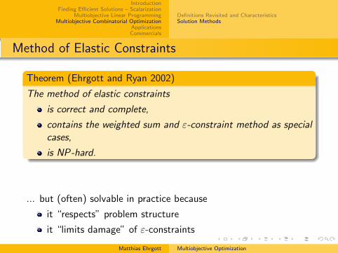
IntroductionFinding Efficient Solutions – Scalarization
Multiobjective Linear ProgrammingMultiobjective Combinatorial Optimization
ApplicationsCommercials
Definitions Revisited and CharacteristicsSolution Methods
Method of Elastic Constraints
Theorem (Ehrgott and Ryan 2002)
The method of elastic constraints
is correct and complete,
contains the weighted sum and ε-constraint method as specialcases,
is NP-hard.
... but (often) solvable in practice because
it “respects” problem structure
it “limits damage” of ε-constraints
Matthias Ehrgott Multiobjective Optimization

IntroductionFinding Efficient Solutions – Scalarization
Multiobjective Linear ProgrammingMultiobjective Combinatorial Optimization
ApplicationsCommercials
Definitions Revisited and CharacteristicsSolution Methods
Integer Programming Duality
Theorem (Klamroth et al. 2004)
x ∈ XE if and only if there isF ∈ F := {F : Rm+p−1 → R nondecreasing}such that x is an optimal solution to
max{
cjx − F ((ckx)k 6=j , b) : Ax 5 b, x = 0, x integer}
.
F can be chosen as an optimal solution of the IP dual
min{
F (−e, b) : F ((−ckx)k 6=j ,Ax) ≥ cjx ∀x ∈ Zn=,F ∈ F
}of max{clx : ckx ≥ εk , k 6= l ,Ax = b, x ∈ Zn
=}The level curve of the objective function of the composite IPat level 0 defines an upper bound on YN .
Matthias Ehrgott Multiobjective Optimization
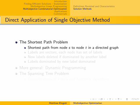
IntroductionFinding Efficient Solutions – Scalarization
Multiobjective Linear ProgrammingMultiobjective Combinatorial Optimization
ApplicationsCommercials
Definitions Revisited and CharacteristicsSolution Methods
Direct Application of Single Objective Method
The Shortest Path Problem
Shortest path from node s to node t in a directed graphLabels are vectors, each node has set of labelsNew labels deleted if dominated by another labelLabels dominated by new label dominated
More general: Dynamic Programming
The Spanning Tree Problem
Generalizations of Prim’s and Kruskal’s algorithms
Matthias Ehrgott Multiobjective Optimization
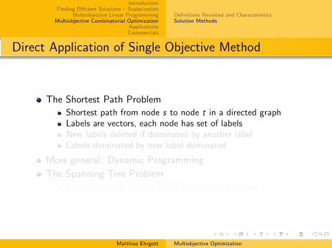
IntroductionFinding Efficient Solutions – Scalarization
Multiobjective Linear ProgrammingMultiobjective Combinatorial Optimization
ApplicationsCommercials
Definitions Revisited and CharacteristicsSolution Methods
Direct Application of Single Objective Method
The Shortest Path Problem
Shortest path from node s to node t in a directed graphLabels are vectors, each node has set of labelsNew labels deleted if dominated by another labelLabels dominated by new label dominated
More general: Dynamic Programming
The Spanning Tree Problem
Generalizations of Prim’s and Kruskal’s algorithms
Matthias Ehrgott Multiobjective Optimization
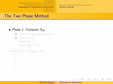
IntroductionFinding Efficient Solutions – Scalarization
Multiobjective Linear ProgrammingMultiobjective Combinatorial Optimization
ApplicationsCommercials
Definitions Revisited and CharacteristicsSolution Methods
The Two Phase Method
Phase 1: Compute XsE
1 Find lexicographic solutions2 Recursively:
Calculate λSolve min
x∈XλTCx
Phase 2: Compute XnE
1 Solve by triangle2 Use neighborhood (wrong)3 Use constraints (bad)4 Use variable fixing (possible)5 Use ranking (good)
0 1 2 3 4 5 6 7 8 9 100
1
2
3
4
5
6
7
8
9
10
Matthias Ehrgott Multiobjective Optimization
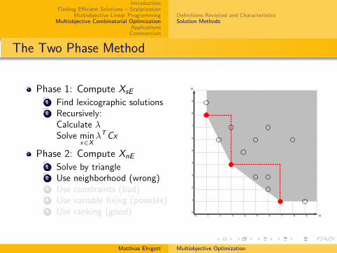
IntroductionFinding Efficient Solutions – Scalarization
Multiobjective Linear ProgrammingMultiobjective Combinatorial Optimization
ApplicationsCommercials
Definitions Revisited and CharacteristicsSolution Methods
The Two Phase Method
Phase 1: Compute XsE
1 Find lexicographic solutions2 Recursively:
Calculate λSolve min
x∈XλTCx
Phase 2: Compute XnE
1 Solve by triangle2 Use neighborhood (wrong)3 Use constraints (bad)4 Use variable fixing (possible)5 Use ranking (good)
0 1 2 3 4 5 6 7 8 9 100
1
2
3
4
5
6
7
8
9
10
Matthias Ehrgott Multiobjective Optimization
IntroductionFinding Efficient Solutions – Scalarization
Multiobjective Linear ProgrammingMultiobjective Combinatorial Optimization
ApplicationsCommercials
Definitions Revisited and CharacteristicsSolution Methods
Enumeration Problems
Finding maximal complete set:
Enumeration to find all optimal solutions of minx∈X λTCxEnumeration to find all x ∈ XnE with Cx = y ∈ YnD
Finding minimal complete set:
Enumeration to find XsE2
Matthias Ehrgott Multiobjective Optimization
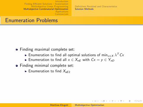

IntroductionFinding Efficient Solutions – Scalarization
Multiobjective Linear ProgrammingMultiobjective Combinatorial Optimization
ApplicationsCommercials
Definitions Revisited and CharacteristicsSolution Methods
Enumeration Problems
Finding maximal complete set:Enumeration to find all optimal solutions of minx∈X λTCxEnumeration to find all x ∈ XnE with Cx = y ∈ YnD
Finding minimal complete set:Enumeration to find XsE2
205
210
215
220
225
230
235
195 200 205 210 215 220 225
z2
z1
( 206,223 )
( 207,222 )
( 208,221 )
( 209,220 )
( 210,219 )
( 211,218 )
( 199,230 )
( 220,209 )
( 218,211 )
( 202,227 )
( 203,226 )
( 204,225 )
( 212,217 )
( 213,216 )
( 214,215 )
( 215,214 )
( 216,213 )
z(x) ∈ ZSN1
z(x) ∈ ZSN2
λ = 0.5666
=0.5λ
=0.4918λ
Matthias Ehrgott Multiobjective Optimization

IntroductionFinding Efficient Solutions – Scalarization
Multiobjective Linear ProgrammingMultiobjective Combinatorial Optimization
ApplicationsCommercials
Definitions Revisited and CharacteristicsSolution Methods
2 Phase Algorithm for Biobjective Assignment
(Przybylski et al. 2004)
Hungarian Method for minx∈X λTCx
Enumeration of all optimal solutions of minx∈X λTCx(Fukuda and Matsui 1992)
Ranking of (non-optimal) solutions of minx∈X λTCx(Chegireddy and Hamacher 1987)
Results for 100× 100:
Range Variable Fixing Seek & Cut Ranking
20 14049.17 2755.75 220.0740 × 17441.35 225.0660 × 38553.18 399.6580 × 53747.45 721.08
100 × 60227.31 711.97
Matthias Ehrgott Multiobjective Optimization

IntroductionFinding Efficient Solutions – Scalarization
Multiobjective Linear ProgrammingMultiobjective Combinatorial Optimization
ApplicationsCommercials
Definitions Revisited and CharacteristicsSolution Methods
The 2 Phase Method for 3 Objectives
Phase 1:
Dichotomic search impossible since normal defined by threenondominated extreme points need not define positive weightsy1 = (11, 11, 14), y2 = (15, 9, 17), y3 = (19, 14, 10) are threenondominated extreme points, normal is (−1, 40, 28)Nondominated extreme point y4 = (13, 16, 11) not found
Phase 2:
Search by triangle impossible due to lack of natural order ofpointsy1 = (22, 42, 25), y2 = (38, 33, 27), y3 = (39, 31, 30) are threenondominated extreme pointsy4 = (30, 38, 37) is not “below” (39,41,30)
Matthias Ehrgott Multiobjective Optimization
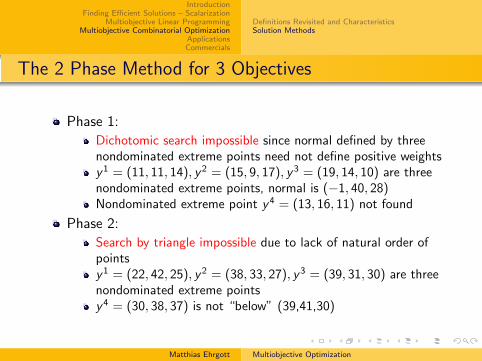
IntroductionFinding Efficient Solutions – Scalarization
Multiobjective Linear ProgrammingMultiobjective Combinatorial Optimization
ApplicationsCommercials
Definitions Revisited and CharacteristicsSolution Methods
The 2 Phase Method for 3 Objectives
Phase 1:
Dichotomic search impossible since normal defined by threenondominated extreme points need not define positive weightsy1 = (11, 11, 14), y2 = (15, 9, 17), y3 = (19, 14, 10) are threenondominated extreme points, normal is (−1, 40, 28)Nondominated extreme point y4 = (13, 16, 11) not found
Phase 2:
Search by triangle impossible due to lack of natural order ofpointsy1 = (22, 42, 25), y2 = (38, 33, 27), y3 = (39, 31, 30) are threenondominated extreme pointsy4 = (30, 38, 37) is not “below” (39,41,30)
Matthias Ehrgott Multiobjective Optimization

IntroductionFinding Efficient Solutions – Scalarization
Multiobjective Linear ProgrammingMultiobjective Combinatorial Optimization
ApplicationsCommercials
Definitions Revisited and CharacteristicsSolution Methods
Weight Set Decomposition
W 0 :=
{λ > 0 : λp = 1−
p∑k=1
λk
}W 0(y) :=
{λ ∈ W 0 : λT y = min{λT y : y ∈ Y }
}Theorem
If y is a nondominated extreme point of Y then dimW 0(y) = p − 1.
W 0(y) =⋃
y∈YsN1W 0(y).
dim W 0(y) + dim F (y) = p − 1 for all y ∈ YsN , where F (y)is the maximal nondominated face of Y containing y.
Matthias Ehrgott Multiobjective Optimization

IntroductionFinding Efficient Solutions – Scalarization
Multiobjective Linear ProgrammingMultiobjective Combinatorial Optimization
ApplicationsCommercials
Definitions Revisited and CharacteristicsSolution Methods
Finding Nondominated Extreme Points
For p = 1, . . . , p find yk
minimizing the k-th objective
S := {y1, . . . , yp} andW 0
p (yk) = {λ ∈ W 0 : λT y =
min{λT y : y ∈ S}}Facets of W 0
p (yk) definebiobjective problems
Solve biobjective problems forall facets for all yk to find newnondominated extreme pointsadded to S
Stop if W 0p (y) = W 0(y) for all
y ∈ S
0
0.2
0.4
0.6
0.8
1
0 0.2 0.4 0.6 0.8 1
λ1
λ2
W0p(y1)
Matthias Ehrgott Multiobjective Optimization

IntroductionFinding Efficient Solutions – Scalarization
Multiobjective Linear ProgrammingMultiobjective Combinatorial Optimization
ApplicationsCommercials
Definitions Revisited and CharacteristicsSolution Methods
Finding Nondominated Extreme Points
For p = 1, . . . , p find yk
minimizing the k-th objective
S := {y1, . . . , yp} andW 0
p (yk) = {λ ∈ W 0 : λT y =
min{λT y : y ∈ S}}Facets of W 0
p (yk) definebiobjective problems
Solve biobjective problems forall facets for all yk to find newnondominated extreme pointsadded to S
Stop if W 0p (y) = W 0(y) for all
y ∈ S
0
0.2
0.4
0.6
0.8
1
0 0.2 0.4 0.6 0.8 1λ1
W0(y1)
λ2
Matthias Ehrgott Multiobjective Optimization

IntroductionFinding Efficient Solutions – Scalarization
Multiobjective Linear ProgrammingMultiobjective Combinatorial Optimization
ApplicationsCommercials
Definitions Revisited and CharacteristicsSolution Methods
Finding Nondominated Extreme Points
For p = 1, . . . , p find yk
minimizing the k-th objective
S := {y1, . . . , yp} andW 0
p (yk) = {λ ∈ W 0 : λT y =
min{λT y : y ∈ S}}Facets of W 0
p (yk) definebiobjective problems
Solve biobjective problems forall facets for all yk to find newnondominated extreme pointsadded to S
Stop if W 0p (y) = W 0(y) for all
y ∈ S
0
0.2
0.4
0.6
0.8
1
0 0.2 0.4 0.6 0.8 1λ1
λ2
W0(y2)
Matthias Ehrgott Multiobjective Optimization

IntroductionFinding Efficient Solutions – Scalarization
Multiobjective Linear ProgrammingMultiobjective Combinatorial Optimization
ApplicationsCommercials
Definitions Revisited and CharacteristicsSolution Methods
Finding Nondominated Extreme Points
For p = 1, . . . , p find yk
minimizing the k-th objective
S := {y1, . . . , yp} andW 0
p (yk) = {λ ∈ W 0 : λT y =
min{λT y : y ∈ S}}Facets of W 0
p (yk) definebiobjective problems
Solve biobjective problems forall facets for all yk to find newnondominated extreme pointsadded to S
Stop if W 0p (y) = W 0(y) for all
y ∈ S
0
0.2
0.4
0.6
0.8
1
0 0.2 0.4 0.6 0.8 1λ1
λ2
W0(y3)
Matthias Ehrgott Multiobjective Optimization

IntroductionFinding Efficient Solutions – Scalarization
Multiobjective Linear ProgrammingMultiobjective Combinatorial Optimization
ApplicationsCommercials
Definitions Revisited and CharacteristicsSolution Methods
Finding Nondominated Extreme Points
For p = 1, . . . , p find yk
minimizing the k-th objective
S := {y1, . . . , yp} andW 0
p (yk) = {λ ∈ W 0 : λT y =
min{λT y : y ∈ S}}Facets of W 0
p (yk) definebiobjective problems
Solve biobjective problems forall facets for all yk to find newnondominated extreme pointsadded to S
Stop if W 0p (y) = W 0(y) for all
y ∈ S
0
0.2
0.4
0.6
0.8
1
0 0.2 0.4 0.6 0.8 1
W0(y4)
λ1
λ2
Matthias Ehrgott Multiobjective Optimization

IntroductionFinding Efficient Solutions – Scalarization
Multiobjective Linear ProgrammingMultiobjective Combinatorial Optimization
ApplicationsCommercials
Definitions Revisited and CharacteristicsSolution Methods
Finding Nondominated Extreme Points
For p = 1, . . . , p find yk
minimizing the k-th objective
S := {y1, . . . , yp} andW 0
p (yk) = {λ ∈ W 0 : λT y =
min{λT y : y ∈ S}}Facets of W 0
p (yk) definebiobjective problems
Solve biobjective problems forall facets for all yk to find newnondominated extreme pointsadded to S
Stop if W 0p (y) = W 0(y) for all
y ∈ S
0
0.2
0.4
0.6
0.8
1
0 0.2 0.4 0.6 0.8 1λ1
λ2
W0(y1)
W0(y2)
W0(y3)
W0(y4)
W0(y5)
Weight to usefor enumeration
Matthias Ehrgott Multiobjective Optimization

IntroductionFinding Efficient Solutions – Scalarization
Multiobjective Linear ProgrammingMultiobjective Combinatorial Optimization
ApplicationsCommercials
Definitions Revisited and CharacteristicsSolution Methods
Finding Supported Nondominated Points
Relevant weights
Intersection points of at leastthree sets W 0(y)Points in the interior of faceswhere two sets W 0(y)intersect
Enumerate all optimal solutionsof weighted sum problems
0
0.2
0.4
0.6
0.8
1
0 0.2 0.4 0.6 0.8 1λ1
λ2
W0(y1)
W0(y2)
W0(y3)
W0(y4)
W0(y5)
Weight to usefor enumeration
Matthias Ehrgott Multiobjective Optimization
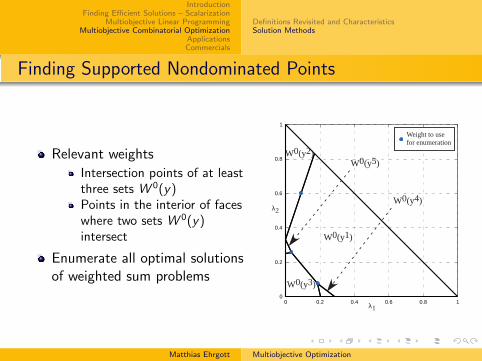
IntroductionFinding Efficient Solutions – Scalarization
Multiobjective Linear ProgrammingMultiobjective Combinatorial Optimization
ApplicationsCommercials
Definitions Revisited and CharacteristicsSolution Methods
Finding Supported Nondominated Points
Relevant weights
Intersection points of at leastthree sets W 0(y)Points in the interior of faceswhere two sets W 0(y)intersect
Enumerate all optimal solutionsof weighted sum problems
0
0.2
0.4
0.6
0.8
1
0 0.2 0.4 0.6 0.8 1λ1
λ2
W0(y1)
W0(y2)
W0(y3)
W0(y4)
W0(y5)
Weight to usefor enumeration
Matthias Ehrgott Multiobjective Optimization
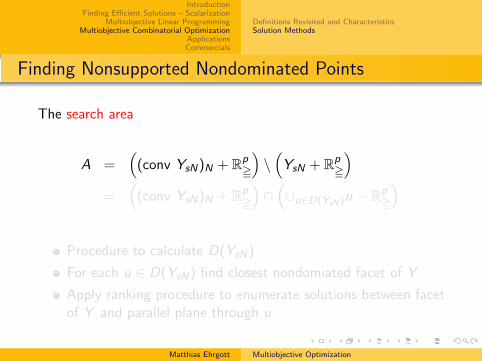
IntroductionFinding Efficient Solutions – Scalarization
Multiobjective Linear ProgrammingMultiobjective Combinatorial Optimization
ApplicationsCommercials
Definitions Revisited and CharacteristicsSolution Methods
Finding Nonsupported Nondominated Points
The search area
A =((conv YsN)N + Rp
=
)\(YsN + Rp
=
)=
((conv YsN)N + Rp
=
)∩(∪u∈D(YsN)u − Rp
=
)
Procedure to calculate D(YsN)
For each u ∈ D(YsN) find closest nondomiated facet of Y
Apply ranking procedure to enumerate solutions between facetof Y and parallel plane through u
Matthias Ehrgott Multiobjective Optimization

IntroductionFinding Efficient Solutions – Scalarization
Multiobjective Linear ProgrammingMultiobjective Combinatorial Optimization
ApplicationsCommercials
Definitions Revisited and CharacteristicsSolution Methods
Results for Three-Objective Assignment Problem
n |YN | S/C 2004 T-P 2003 L et al. (2005) P et al. 20075 12 0.15 0.04 0.15 0.00
10 221 99865.00 97.30 41.70 0.0815 483 × 544.53 172.29 0.3620 1942 × × 1607.92 4.5125 3750 × × 5218.00 30.1330 5195 × × 15579.00 55.8735 10498 × × 101751.00 109.9640 14733 × × × 229.0545 23941 × × × 471.6050 29193 × × × 802.68
Matthias Ehrgott Multiobjective Optimization
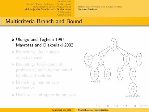
IntroductionFinding Efficient Solutions – Scalarization
Multiobjective Linear ProgrammingMultiobjective Combinatorial Optimization
ApplicationsCommercials
Definitions Revisited and CharacteristicsSolution Methods
Multicriteria Branch and Bound
Ulungu and Teghem 1997,Mavrotas and Diakoulaki 2002
Branching: As in singleobjective case
Bounding: Ideal point ofproblem at node is dominatedby efficient solution
Branching may be veryineffective
Use lower and upper bound sets
N0
∅
∅
N1
1, 2, 3
∅
N2
1, 2
3
N5
1
2
N9
∅
1
N3
1, 2, 4
3
N4
1, 2
3, 4
N6
1, 3
2
N7
1
2, 3
N8
1, 4, 5
2, 3
L ={(
23
27
)}
L ={(
23
27
)
,(
29
16
)}
L ={(
23
27
)
,(
29
16
)
,(
27
18
)}
Matthias Ehrgott Multiobjective Optimization
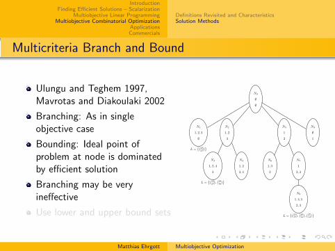
IntroductionFinding Efficient Solutions – Scalarization
Multiobjective Linear ProgrammingMultiobjective Combinatorial Optimization
ApplicationsCommercials
Definitions Revisited and CharacteristicsSolution Methods
Multicriteria Branch and Bound
Ulungu and Teghem 1997,Mavrotas and Diakoulaki 2002
Branching: As in singleobjective case
Bounding: Ideal point ofproblem at node is dominatedby efficient solution
Branching may be veryineffective
Use lower and upper bound sets
N0
∅
∅
N1
1, 2, 3
∅
N2
1, 2
3
N5
1
2
N9
∅
1
N3
1, 2, 4
3
N4
1, 2
3, 4
N6
1, 3
2
N7
1
2, 3
N8
1, 4, 5
2, 3
L ={(
23
27
)}
L ={(
23
27
)
,(
29
16
)}
L ={(
23
27
)
,(
29
16
)
,(
27
18
)}
Matthias Ehrgott Multiobjective Optimization
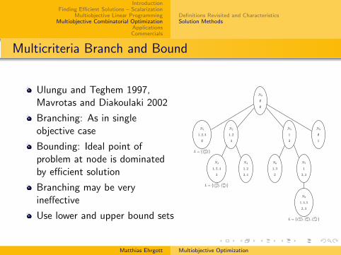
IntroductionFinding Efficient Solutions – Scalarization
Multiobjective Linear ProgrammingMultiobjective Combinatorial Optimization
ApplicationsCommercials
Definitions Revisited and CharacteristicsSolution Methods
Multicriteria Branch and Bound
Ulungu and Teghem 1997,Mavrotas and Diakoulaki 2002
Branching: As in singleobjective case
Bounding: Ideal point ofproblem at node is dominatedby efficient solution
Branching may be veryineffective
Use lower and upper bound sets
N0
∅
∅
N1
1, 2, 3
∅
N2
1, 2
3
N5
1
2
N9
∅
1
N3
1, 2, 4
3
N4
1, 2
3, 4
N6
1, 3
2
N7
1
2, 3
N8
1, 4, 5
2, 3
L ={(
23
27
)}
L ={(
23
27
)
,(
29
16
)}
L ={(
23
27
)
,(
29
16
)
,(
27
18
)}
Matthias Ehrgott Multiobjective Optimization

IntroductionFinding Efficient Solutions – Scalarization
Multiobjective Linear ProgrammingMultiobjective Combinatorial Optimization
ApplicationsCommercials
Definitions Revisited and CharacteristicsSolution Methods
Bound Sets
Ehrgott and Gandibleux 2005:1 Lower bound set L
is Rp=-closed
is Rp=-bounded
YN ⊂ L + Rp=
L ⊂(L + Rp
=
)N
2 Upper bound set U
is Rp=-closed
is Rp=-bounded
YN ∈ cl[(
U + Rp=
)c]U ⊂
(U + Rp
=
)N
0 1 2 3 4 5 6 7 8 9 100
1
2
3
4
5
6
7
8
9
10
Matthias Ehrgott Multiobjective Optimization
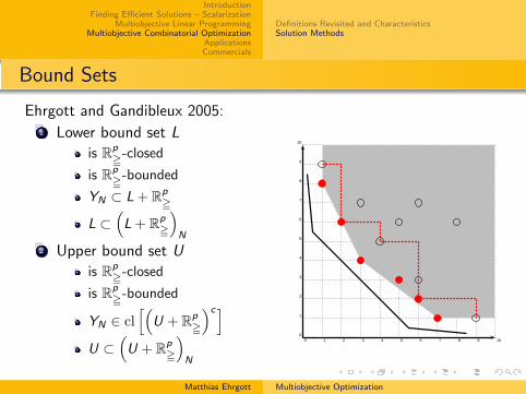

IntroductionFinding Efficient Solutions – Scalarization
Multiobjective Linear ProgrammingMultiobjective Combinatorial Optimization
ApplicationsCommercials
Definitions Revisited and CharacteristicsSolution Methods
10000
20000
30000
40000
50000
60000
70000
80000
90000
10000 20000 30000 40000 50000 60000 70000 80000 90000
y2
y1
ub
⋆
⋆⋆
⋆
⋆⋆⋆
⋆⋆
⋆⋆⋆⋆
⋆⋆⋆⋆⋆⋆⋆⋆⋆⋆⋆⋆⋆⋆⋆⋆ ⋆⋆ ⋆⋆⋆⋆⋆ ⋆ ⋆⋆ ⋆ ⋆ ⋆
⋆
lb
r
r
r
rrrrrrrrrrrrrrr r
r
rrrrrrr rrrrr rr r
r
dMax
e
e
e
Matthias Ehrgott Multiobjective Optimization

IntroductionFinding Efficient Solutions – Scalarization
Multiobjective Linear ProgrammingMultiobjective Combinatorial Optimization
ApplicationsCommercials
Portfolio Selection
Markowitz 1952 with cardinality constraint, e.g. Chang et al. 2000
max z1(x) = µT x
min z2(x) = xTσx
subject to eT x = 1
xi 5 uiyi
xi = liyi
eT y = k
y ∈ {0, 1}n
0
50
100
150
200
250
300
350
0 200 400 600 800 1000 1200 1400 1600f 1
f2
Matthias Ehrgott Multiobjective Optimization
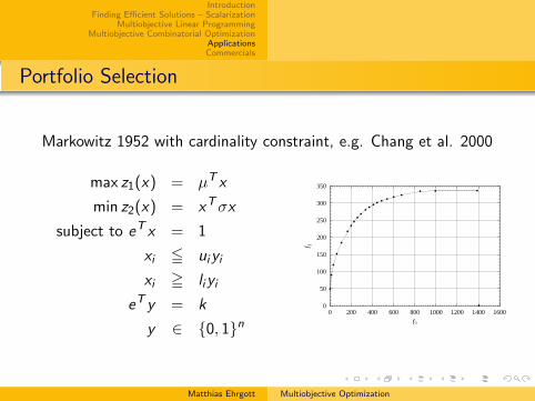
IntroductionFinding Efficient Solutions – Scalarization
Multiobjective Linear ProgrammingMultiobjective Combinatorial Optimization
ApplicationsCommercials
Portfolio Selection
Markowitz 1952 with cardinality constraint, e.g. Chang et al. 2000
max z1(x) = µT x
min z2(x) = xTσx
subject to eT x = 1
xi 5 uiyi
xi = liyi
eT y = k
y ∈ {0, 1}n
0
50
100
150
200
250
300
350
0 200 400 600 800 1000 1200 1400 1600f 1
f2
Matthias Ehrgott Multiobjective Optimization

IntroductionFinding Efficient Solutions – Scalarization
Multiobjective Linear ProgrammingMultiobjective Combinatorial Optimization
ApplicationsCommercials
Airline Crew Scheduling
Partition flights into set of pairings, but minimizing cost can causedelays ...and be very expensive
Sunday, 4 August, 2002, 20:29 GMT 21:29 UK
Delays as Easyjet cancels 19 flights
Passengers with low-cost airline Easyjet are suffering delays after 19 flights in and out
of Britain were cancelled.
The company blamed the move - which comes a week after passengers staged a protest sit-in
at Nice airport - on crewing problems stemming from technical hitches with aircraft.
Crews caught up in the delays worked up to their maximum hours and then had to be allowed
home to rest.
Mobilising replacement crews has been a problem as it takes time to bring people to
airports from home. Standby crews were already being used and other staff are on holiday.
Matthias Ehrgott Multiobjective Optimization

IntroductionFinding Efficient Solutions – Scalarization
Multiobjective Linear ProgrammingMultiobjective Combinatorial Optimization
ApplicationsCommercials
Airline Crew Scheduling
Model 1: Minimize cost and minimize non-robustness (Ehrgott andRyan 2002)
aij =
{1 pairing j includes flight i0 otherwise
min z1(x) = cT x
min z2(x) = rT x
subject to Ax = e
Mx = b
x ∈ {0, 1}n
Matthias Ehrgott Multiobjective Optimization
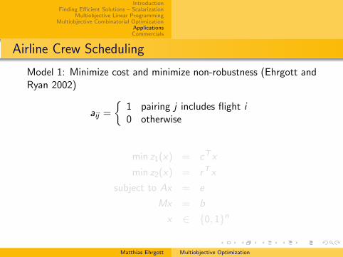
IntroductionFinding Efficient Solutions – Scalarization
Multiobjective Linear ProgrammingMultiobjective Combinatorial Optimization
ApplicationsCommercials
Airline Crew Scheduling
Model 1: Minimize cost and minimize non-robustness (Ehrgott andRyan 2002)
aij =
{1 pairing j includes flight i0 otherwise
min z1(x) = cT x
min z2(x) = rT x
subject to Ax = e
Mx = b
x ∈ {0, 1}n
Matthias Ehrgott Multiobjective Optimization

IntroductionFinding Efficient Solutions – Scalarization
Multiobjective Linear ProgrammingMultiobjective Combinatorial Optimization
ApplicationsCommercials
0
1000
2000
3000
4000
5000
6000
880 900 920 940 960 980 1000 1020 1040Cost
Non
-rob
ustn
ess
LPIP 2% bound gap
Cost IP solution 2% bound gap
Matthias Ehrgott Multiobjective Optimization

IntroductionFinding Efficient Solutions – Scalarization
Multiobjective Linear ProgrammingMultiobjective Combinatorial Optimization
ApplicationsCommercials
Radiotherapy Treatment Design
Choose beam directions and intensities to destroy tumour andspare healthy organs (e.g. Holder 2004)
min(zT , zS , zN )subject to AT x + zT e = lT
AT x 5 uTASx − zSe 5 uS
AN x − zN e 5 uNzS = −uSzN = 0
x = 0x 5 Myey ∈ {0, 1}n
Matthias Ehrgott Multiobjective Optimization

IntroductionFinding Efficient Solutions – Scalarization
Multiobjective Linear ProgrammingMultiobjective Combinatorial Optimization
ApplicationsCommercials
Radiotherapy Treatment Design
Choose beam directions and intensities to destroy tumour andspare healthy organs (e.g. Holder 2004)
min(zT , zS , zN )subject to AT x + zT e = lT
AT x 5 uTASx − zSe 5 uS
AN x − zN e 5 uNzS = −uSzN = 0
x = 0x 5 Myey ∈ {0, 1}n 5 10 15 20 25 30 35 40 45 50
5
10
15
20
25
30
35
40
45
50
Matthias Ehrgott Multiobjective Optimization

IntroductionFinding Efficient Solutions – Scalarization
Multiobjective Linear ProgrammingMultiobjective Combinatorial Optimization
ApplicationsCommercials
Matthias Ehrgott Multiobjective Optimization

IntroductionFinding Efficient Solutions – Scalarization
Multiobjective Linear ProgrammingMultiobjective Combinatorial Optimization
ApplicationsCommercials
19th International Conference onMultiple Criteria Decision Making
MCDM for Sustainable Energy and Transportation Systems
7th – 12th January 2008The University of Auckland, Auckland, New Zealand
Deadline for abstract submission September 30, 2007Deadline for early registration October 15, 2007
www.esc.auckland.ac.nz/[email protected]
MCDM
mcdmposter.indd 1 3/26/2007 16:34:59Matthias Ehrgott Multiobjective Optimization


![Multiobjective optimization for pavement maintenance and rehabilitation programming ... · 2019. 7. 9. · Integer programming [4], optimal control theory [5], non-linear programming](https://static.fdocuments.net/doc/165x107/60b63cc728707f56fa4ed021/multiobjective-optimization-for-pavement-maintenance-and-rehabilitation-programming.jpg)