Multiobjective genetic programming for maximizing ROC

Neurocomputing ] (]]]]) ]]]–]]]

Contents lists available at SciVerse ScienceDirect

Neurocomputing

0925-23

http://d

n Corr

E-m

ketang@

Pleas

journal homepage: www.elsevier.com/locate/neucom

Multiobjective genetic programming for maximizing ROC performance

Pu Wang a, Ke Tang a,n, Thomas Weise a, E.P.K. Tsang b, Xin Yao c

a Nature Inspired Computation and Applications Laboratory (NICAL), School of Computer Science and Technology, University of Science and Technology of China (USTC),

Hefei, Anhui 230027, Chinab Department of Computer Science, University of Essex, Wivenhoe Park, Colchester CO4 3SQ, UKc Center of Excellence for Research in Computational Intelligence and Applications (CERCIA), School of Computer Science, The University of Birmingham Edgbaston,

Birmingham B15 2TT, UK

a r t i c l e i n f o

Keywords:

Classification

ROC analysis

AUC

ROCCH

Genetic programming

Evolutionary multiobjective algorithm

Memetic algorithm

Decision tree

12/$ - see front matter & 2013 Elsevier B.V. A

x.doi.org/10.1016/j.neucom.2012.06.054

esponding author.

ail addresses: [email protected] (P

ustc.edu.cn (K. Tang).

e cite this article as: P. Wang, et al.

a b s t r a c t

In binary classification problems, receiver operating characteristic (ROC) graphs are commonly used for

visualizing, organizing and selecting classifiers based on their performances. An important issue in the

ROC literature is to obtain the ROC convex hull (ROCCH) that covers potentially optima for a given set of

classifiers [1]. Maximizing the ROCCH means to maximize the true positive rate (tpr) and minimize the

false positive rate (fpr) for every classifier in ROC space, while tpr and fpr are conflicting with each

other. In this paper, we propose multiobjective genetic programming (MOGP) to obtain a group of

nondominated classifiers, with which the maximum ROCCH can be achieved. Four different multi-

objective frameworks, including Nondominated Sorting Genetic Algorithm II (NSGA-II), Multiobjective

Evolutionary Algorithms Based on Decomposition (MOEA/D), Multiobjective selection based on

dominated hypervolume (SMS-EMOA), and Approximation-Guided Evolutionary Multi-Objective

(AG-EMOA) are adopted into GP, because all of them are successfully applied into many problems

and have their own characters. To improve the performance of each individual in GP, we further

propose a memetic approach into GP by defining two local search strategies specifically designed for

classification problems. Experimental results based on 27 well-known UCI data sets show that MOGP

performs significantly better than single objective algorithms such as FGP, GGP, EGP, and MGP, and

other traditional machine learning algorithms such as C4.5, Naive Bayes, and PRIE. The experiments

also demonstrate the efficacy of the local search operator in the MOGP framework.

& 2013 Elsevier B.V. All rights reserved.

1. Introduction

Classification [2] is one of the most important areas inmachine learning. Here, the goal is to find assignments of classesto un-classified and unseen instances (data samples) based oninformation previously learned. In the most common case,referred to as binary classification, there are two classes orcategories and all instances in a data set belong to one of them.Solving classification problems basically means to design goodclassifier(s) which make right assignments as often as possible.

One open question is how to measure the performance of aclassifier. If classifiers are synthesized with optimization algo-rithms, the choice of the performance measure will have tremen-dous impact on the results that we will obtain. Simpleclassification accuracy, though being used as the performancemetric for a long time, is actually not a good choice [3]. The

ll rights reserved.

. Wang),

, (2013), http://dx.doi.org/1

receiver operating characteristics, or ROC for short, has beenclaimed as a generally useful performance visualizing methodbecause its properties are not sensitive to skewed class distribu-tions or unequal misclassification costs, two characteristics whichare known to have a negative impact on the utility of the accuracymeasure.

The ROC graph is a technique for visualizing, organizing andselecting classifiers based on their performance [1]. It has beenwidely used in signal detection [4], medical decision making [5],and other fields over the course of the past 40 years. In recentyears, because of the ever-increasing use of ROC graphs in themachine learning community, the ROC analysis became a centraltechnique for tackling classification problems. The ROC curve, animportant topic in ROC analysis, is obtained by varying discrimi-native thresholds over the output of a classifier [1]. The areaunder the ROC curve (AUC) is accepted as a fair indicator tomeasure the classifier performance for binary classification, sinceit is invariant to operating conditions such as different misclassi-fication costs and skewed class distributions [6]. ROCCH, anotherimportant topic in classification problems, represents the convexhull of a set of points (hard classifiers) obtained from several

0.1016/j.neucom.2012.06.054i

www.elsevier.com/locate/neucom

www.elsevier.com/locate/neucom

http://dx.doi.org/10.1016/j.neucom.2012.06.054



mailto:[email protected]

mailto:[email protected]





edward

Typewritten Text

Available online 1 March 2013 http://www.sciencedirect.com/science/article/pii/S0925231213001938

P. Wang et al. / Neurocomputing ] (]]]]) ]]]–]]]2

curves (i.e., soft classifiers) [7]. A classifier is potentially optimal ifand only if it touches the ROCCH. Otherwise, we can always find abetter classifier. It is possible to get a potentially optimal classifierin ROCCH even if the data sets have skewed class distributions ormisclassification costs. Actually, we can consider the ROC curve asa special ROCCH when there is only a single soft classifier. Thismeans that ROCCH could work more powerfully than a plain ROCcurve. Consequently, we mainly consider the ROCCH in this paperand we will focus on searching a group of classifiers not only tomaximize the ROCCH performance but also try to maximize theAUC of a single soft classifier in binary classification problems.

In this paper, we utilize GP combined with multiobjectivetechniques to approximate the optimal ROCCH. This work empiri-cally investigates multiobjective genetic programming (MOGP)with four different frameworks on binary classification problems.We show that local search strategies can play a key role in GP forclassification problems and that special local search operators canimprove the performance.

This paper is organized as follows: Section 2 outlines therelated work and in Section 3, we introduce the background andbasic algorithms used in our research. Section 4 will describe ourframework to classification problems and presents local searchoperators working in GP. Experiments are studied in Section 5where four research questions are answered. Section 6 providesthe conclusion and a discussions on the important aspects andfuture perspectives of this work.

2. Related work

2.1. ROCCH in classification

The roots of ROCCH maximization problems can be traced backto [7]. In that work, iso-performance lines1 are translated byoperating conditions of classifiers and used to identify a portionof the ROCCH, by which we can choose suitable classifiers for datasets with different skewed class distribution or misclassificationcosts. In [8], a combination of rule sets to produce instance scoresindicating the likelihood that an instance belongs to a given classis described.

Flach et al. [9] investigated a method to detect and repairconcavities in ROC curves. The basic idea here is that if a point liesbelow the line spanned by two other points in ROC, then it can bemirrored to a better point which could perform well beyond theoriginal ROC curve. This can be used to expand the ROCCH. Prati[10] introduced a rule selection algorithm based on ROC analysisto find minimal rule sets with compatible AUC values. Here,selection is based on whether a rule can improve thecurrent ROCCH.

In [11], a method which takes Neyman–Pearson lemma [12] asthe theoretical basis for finding the optimal combination ofclassifiers to maximize the ROCCH is given. Fawcett [13] presentsa method for learning rules directly from ROC space. This methodutilizes the geometrical properties of the ROC to generate newrules to maximize the ROC performance. Essentially, all aboveworks are searching a rule sets to maximize ROCCH.

2.2. Genetic programming for classification

Genetic programming (GP) [14] is a branch of evolutionaryalgorithms (EAs). Standard GP has a tree-like representationwhich can be generated by modular, grammatical, and

1 All classifiers corresponding to the points on one line have the same

expected costs.

Please cite this article as: P. Wang, et al., (2013), http://dx.doi.org/1

developmental methods [15]. Tree-based classifiers have a longtradition in machine learning. They are considered to be moreexplicit, intuitive, and interpretable than, e.g., neural networks.GP therefore has widely been used for solving classificationproblems [16,17].

An example of using GP to evolve regression rules for a data setwith intertwined spirals pattern is already given in Koza’s 1992book [14]. Another early work [18] used in image recognition dates20 years back. In the area of data mining, GP has been applied mostsuccessful in two particular fields: one is classification for data setswith different misclassification costs, as GP is suitable for cost-sensitive learning. [19], e.g., focused on financial forecasting pro-blems by consolidating two types of misclassification errors into asingle objective function. GP involving cost-sensitive learning hasfurthermore been adopted in filtering junk E-mail [20].

The second field is classification of imbalanced data sets, i.e.,data sets where one class occurs much more often than theother—one of the areas where the accuracy metric may becomeuseless. Ref. [21] adopts GP to bankruptcy prediction, a primeexample for this issue as there are significantly more solventfirms than defaulting ones. Patterson [22] gave a new fitnessfunction for GP applied on highly imbalanced database. Moreover,Bhowan et al. [23] proposed a multiobjective genetic program-ming approach to evolving accurate and diverse ensembles ofgenetic program classifiers with good performance on both theminority and majority classes.

Many technologies have been combined with GP to improvethe classification performance in these two fields, ranging fromensemble learning over multiobjective methods to local searchstrategies. As both imbalanced problems and different misclassi-fication costs can be included in the ROCCH [7], this work willfocus on GP for maximizing the ROCCH. It should further bementioned that there is a strong analogy of ROCCH and the Paretofront in multiobjective optimization [24].

In this paper, we use multiobjective GP (MOGP) to approx-imate the optimal ROCCH. We empirically investigate MOGP withfour different frameworks on binary classification problems.Additionally, we show that local search strategies can play a keyrole in GP for classification problems as special local searchoperators can carefully be designed to improve the performance.

3. ROCCH, classification, and multiobjective optimization

3.1. Overview of ROCCH in classification problems

3.1.1. ROC Graph and ROCCH

In binary classification problems, each instance I in the data setis marked a certain label from the set {p, n} of positive andnegative class labels. A classifier is a mapping from instances topredicted classes, and accuracy is the most commonly usedevaluation measure. However, its disadvantage are known for along time [25]. Generally, accuracy is not a suitable metric for costsensitive and skewed class distribution classification problems. Toovercome the weakness of accuracy, ROC analysis has beenintroduced in machine learning. Ref. [26] demonstrated the valueof ROC curves in evaluating and comparing algorithms. Animportant tool of ROC analysis is the ROC graph which is usedto visualize the performance of classifiers. The X-axis and Y-axisof ROC graphs display the true positive rate(tpr) and false positiverate (fpr). The performance of a hard or discrete classifier on a dataset can be mapped in a single point in this graph. The upper leftpoint (0,1) represents a perfect classifier which predicts positive(or Yes) to all positive instances and negative (or No) to allnegative instances. The points in lower right area are conservativeclassifiers which produce more negative labels than positive

0.1016/j.neucom.2012.06.054i




Fig. 2. Find optimal classifiers in ROCCH.

P. Wang et al. / Neurocomputing ] (]]]]) ]]]–]]] 3

labels. In contrast, the points in upper right area are liberalclassifiers. All the points along the diagonal are totally randomclassifier and all classifiers below the diagonal have worse-than-random performance. A soft classifier which produces a contin-uous output (e.g. an estimate of an instance’s class membershipprobability) can be mapped in a set of points by varying thethreshold. These points then form a ROC curve.

The ROCCH is the convex hull of the set of points in ROC space.These can be obtained from discrete classifiers and soft classifiersalike. The ROC curve of a soft classifier can directly be consideredas a ROCCH if there is only one soft classifier. The right side ofFig. 1 shows a convex hull over three different ROC curves. Scott[27] and Fawcett [1] have pointed out that two existing classifierscan be used to create a realizable classifier whose performance(in terms of ROC) lies on the line of connecting the performance ofits two endpoints. Hence, any classifiers whose performances arebelow the ROC convex hull could be defeated by realizableclassifiers. A demonstration is shown on the right side of Fig. 1.There are two realizable classifiers whose performance (point b

and c) are better than the performance of point a, which is underthe ROC convex hull. Point b has the same fpr with point a, but itstpr is higher. Point c has the same tpr with a, but its fpr is lower.More generally, all the classifiers whose performances are underthe convex hull are not optimal. In other words, a classifier ispotentially optimal if and only if it lies on the convex hull of theset of points in ROC space [1].

In the following, we will give an example of using ROCCH tosearch optimal points for different situations such as data setswith different error costs and class distributions. One importanttarget of classification problems is to minimize the total errorcosts. Suppose cðY,nÞ is the cost of a false positive error, cðN,pÞ isthe cost of a false negative error, and Ntr is the number of totalinstances. The class distributions of the data set are noted by theclasses’ a priori probabilities pðpÞ and pðnÞ ¼ 1�pðpÞ. The totalerror costs can be represented as

Cost¼Ntr � pðnÞ � fpr � cðY,nÞþNtr � pðpÞ � ð1�tprÞ � cðN,pÞ ð1Þ

If there are two points ðtpr1,fpr1Þ and ðtpr2,fpr2Þ that have thesame total error costs, we can get the following equation:

tpr1�tpr2

fpr1�fpr2¼

cðY,nÞpðnÞ

cðN,pÞpðpÞ¼m ð2Þ

In Eq. (2), m is defined as a slope of an iso-performance line in [7].In other words, all the classifiers corresponding to the points onan iso-performance line have the same expected cost. Moreover,each set of class and cost distributions (the middle term of above

Fig. 1. ROC Graph


equation) defines a family of iso-performance lines. Moving theiso-performance line until it gets in contact with a point inROCCH, the joint point with a larger tpr-intercept (means thetpr-intercept of the line determined by joint point and the slop inROC graph) represents a classifier which can produce lowerexpected cost.

In Fig. 2, there are two iso-performance lines: a with m¼10 andline b with m¼0.1. Imagine a scenario where the data set has a classdistribution where the negatives outnumber the positives by 10 to 1,but the costs of false positives equal to the false negative costs. Aclassifier with performance at C1 is suitable for this data set andachieves the minimal expected cost in this ROCCH. Consider anotherscenario in which a data set has a balanced class distribution, butthe problem is very cost sensitive. If a false negative is 10 times asexpensive as false positive, the suitable classifier is located at C2which is on the iso-performance line b with m¼0.1.

3.2. ROCCH and multiobjective problems

Essentially, the ROCCH maximization problem aims at findinga set of classifiers to approximate the upmost line and the

and ROCCH.

0.1016/j.neucom.2012.06.054i




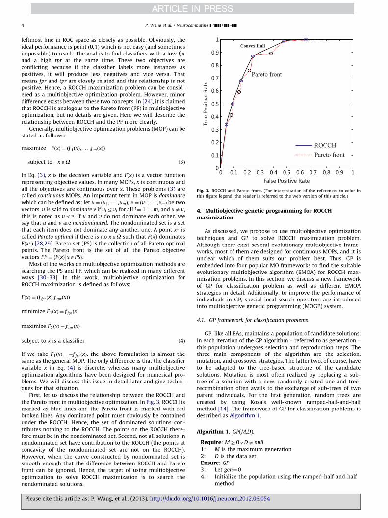
Fig. 3. ROCCH and Pareto front. (For interpretation of the references to color in

this figure legend, the reader is referred to the web version of this article.)


leftmost line in ROC space as closely as possible. Obviously, theideal performance is point ð0,1Þ which is not easy (and sometimesimpossible) to reach. The goal is to find classifiers with a low fpr

and a high tpr at the same time. These two objectives areconflicting because if the classifier labels more instances aspositives, it will produce less negatives and vice versa. Thatmeans fpr and tpr are closely related and this relationship is notpositive. Hence, a ROCCH maximization problem can be consid-ered as a multiobjective optimization problem. However, minordifference exists between these two concepts. In [24], it is claimedthat ROCCH is analogous to the Pareto front (PF) in multiobjectiveoptimization, but no details are given. Here we will describe therelationship between ROCCH and the PF more clearly.

Generally, multiobjective optimization problems (MOP) can bestated as follows:

maximize FðxÞ ¼ ðf 1ðxÞ, . . . ,f mðxÞÞ

subject to xAO ð3Þ

In Eq. (3), x is the decision variable and F(x) is a vector functionrepresenting objective values. In many MOPs, x is continuous andall the objectives are continuous over x. These problems (3) arecalled continuous MOPs. An important term in MOP is dominance

which can be defined as: let u¼ ðu1, . . . ,umÞ, v¼ ðv1, . . . ,vmÞ be twovectors, u is said to dominate v if uirvi for all i¼ 1 . . .m, and uav,this is noted as u!v. If u and v do not dominate each other, wesay that u and v are nondominated. The nondominated set is a setthat each item does not dominate any another one. A point x% iscalled Pareto optimal if there is no xAO such that F(x) dominatesFðx%Þ [28,29]. Pareto set (PS) is the collection of all Pareto optimalpoints. The Pareto front is the set of all the Pareto objectivevectors PF ¼ fFðxÞ9xAPSg.

Most of the works on multiobjective optimization methods aresearching the PS and PF, which can be realized in many differentways [30–33]. In this work, multiobjective optimization forROCCH maximization is defined as follows:

FðxÞ ¼ ðf fprðxÞ,f tprðxÞÞ

minimize F1ðxÞ ¼ f fprðxÞ

maximize F2ðxÞ ¼ f tprðxÞ

subject to x is a classifier ð4Þ

If we take F1ðxÞ ¼�f fprðxÞ, the above formulation is almost thesame as the general MOP. The only difference is that the classifiervariable x in Eq. (4) is discrete, whereas many multiobjectiveoptimization algorithms have been designed for numerical pro-blems. We will discuss this issue in detail later and give techni-ques for that situation.

First, let us discuss the relationship between the ROCCH andthe Pareto front in multiobjective optimization. In Fig. 3, ROCCH ismarked as blue lines and the Pareto front is marked with redbroken lines. Any dominated point must obviously be containedunder the ROCCH. Hence, the set of dominated solutions con-tributes nothing to the ROCCH. The points on the ROCCH there-fore must be in the nondominated set. Second, not all solutions innondominated set have contribution to the ROCCH (the points atconcavity of the nondominated set are not on the ROCCH).However, when the curve constructed by nondominated set issmooth enough that the difference between ROCCH and Paretofront can be ignored. Hence, the target of using multiobjectiveoptimization to solve ROCCH maximization is to search thenondominated solutions.


4. Multiobjective genetic programming for ROCCHmaximization

As discussed, we propose to use multiobjective optimizationtechniques and GP to solve ROCCH maximization problem.Although there exist several evolutionary multiobjective frame-works, most of them are designed for continuous MOPs, and it isunclear which of them suits our problem best. Thus, GP isembedded into four popular MO frameworks to find the suitableevolutionary multiobjective algorithm (EMOA) for ROCCH max-imization problems. In this section, we discuss a new frameworkof GP for classification problem as well as different EMOAstrategies in detail. Additionally, to improve the performance ofindividuals in GP, special local search operators are introducedinto multiobjective genetic programming (MOGP) system.

4.1. GP framework for classification problems

GP, like all EAs, maintains a population of candidate solutions.In each iteration of the GP algorithm – referred to as generation –this population undergoes selection and reproduction steps. Thethree main components of the algorithm are the selection,mutation, and crossover strategies. The latter two, of course, haveto be adapted to the tree-based structure of the candidatesolutions. Mutation is most often realized by replacing a sub-tree of a solution with a new, randomly created one and tree-recombination often avails to the exchange of sub-trees of twoparent individuals. For the first generation, random trees arecreated by using Koza’s well-known ramped-half-and-halfmethod [14]. The framework of GP for classification problems isdescribed as Algorithm 1.

Algorithm 1. GP(M,D).

0.1016

Require: MZ03Danull

1:
M is the maximum generation 2: D is the data set Ensure: GP
3:
Let gen¼0 4: Initialize the population using the ramped-half-and-half
method

/j.neucom.2012.06.054i




Fo


5:

ig. 5. T

perator

Pleas

while genrM do
6: Evaluate fitness of each individual 7: Update the best individual 8: Survival Selection þ Crossover Operation 9: Mutation Operation 10: gen¼gen þ 1 11: end while
4.1.1. Tree-based individuals for classification

Discriminant functions, classification rules, and decision treesare three common tree-based classifier structures that can besynthesized with GP. If an n-class classifier is to be found, eithern�1 discriminant functions or classification rules or n�1 thresh-olds for a single discriminant function are needed. Because of thelack of logical conjunctions such as AND, OR, NOT, off-the-shelfdecision trees are highly redundant. Fig. 4 shows a geneticdecision tree (GDT) [34] that combines a decision trees andclassification rules. Besides, a backus normal form (BNF) grammar[35] for GDTs can be defined, which makes it more convenient to

Fig. 4. Genetic decision tree for classification.

ree based crossover is shown on the left side, two subtrees are selected and

which swaps two subtrees from the same individual.

e cite this article as: P. Wang, et al., (2013), http://dx.doi.org/1

generate GDT individuals with GP. In a GDT, Ai and Cj are theindex of features and index of labels in the input data set,respectively, where 0r ir9A9, 9A9 is number of features and0r jr9C9, 9C9 is number of labels (Fig. 5).

4.2. Multiobjective genetic programming

In this section, we will introduce multiobjective geneticprogramming to maximize the ROC performance in classificationproblems. There exist many efficient evolutionary multiobjectivealgorithms invented to solve continuous function optimizationproblems. It is, however, unclear which one is more suitable forGP for classification problems. Therefore, we conduct an in-depthstudy to identify the most appropriate framework.

4.2.1. Evolutionary multiobjective algorithms

We take four EMOAs into consideration: NSGA-II [30], MOEA/D[31], SMS-EMOA [36], and AGEMOA [33]. The most importantfactor in EMOAs is the strategy used to rank the individuals in thepopulation, in other words, the survival mechanism. The reason ofwhy we choose these EMOAs is that all of them adopt differentmultiobjective frameworks which employ different metrics intrading off conflicting objectives. Since we do not know which isbest for ROCCH maximization, we aim for maximizing thediversity in our experiments.

A fast and elitist multiobjective genetic algorithm, whichbased on nondominated sorting, called NSGA-II, is introduced in[30]. The main contribution of NSGA-II is that it defines a methodto rank the individuals by dominance depth and crowdingdistance. NSGA-II is used here as representative of algorithmsthat use dominance relationships, i.e., that mainly focus on thedominance count and rank. There are other algorithms such asSPEA [37] and SPEA-II [38] with roughly similar structure.

Multiobjective evolutionary algorithm based on decomposi-tion (MOEA/D) [31] decomposes a multiobjective optimizationproblem into a number of scalar optimization subproblems andoptimizes them simultaneously. The basic idea of MOEA/D is thatone solution for a subproblem can use the information providedby its neighbors to improve its performance. Because of that

swapped between different two individuals. The right side shows the mutation

0.1016/j.neucom.2012.06.054i





character, MOEA/D has a lower computational complexity thanNSGA-II.

The hypervolume is a quality metric frequently used inevolutionary approaches to multiobjective optimization pro-blems. SMS-EMOA [36] applies a multiobjective selectionmechanism based on the hypervolume measure combined withthe concept of nondominated sorting. An individual will survivewith a higher probability if it makes higher contribution to thehypervolume covered by the current estimate of the Pareto front.

Bringmann et al. [33] pointed out that the dominance relationand other measures were used to ensure diversity in objectivespace but are not guided by a formal notion of approximation. Inthat work, they proposed a measure (approximate distance) todefine the additive approximation of one nondominated set to thetarget set. The selection mechanism in evolutionary optimizationis that an individual will survive with higher probability when ithas higher contribution to reduce the approximate distance.

4.2.2. Operators used in MOGP

(1) Tree based crossover and mutation: First of all, we willoutline the search operators used in GP, i.e., the unary mutationoperation and the binary crossover operator [15,14,29]. In thecrossover operator, one subtree is random selected from each ofthe two parent solutions. The selected subtrees are then swapped.The most commonly used mutation operation randomly selects anode in a tree and then substitutes the subtree rooted there witha randomly generated one. Another possible mutation operationrandomly selects two subtrees from a parent and swaps them.Though tree based mutation operators have been used often in GPworks, they may not work very efficiently in classificationproblems because randomly re-generated subtree-based muta-tion ignores the information obtained by its parent which is atrained individual. We will introduce tailor-made operators forthis domain in the following.

(2) Decision tree-based local search strategies: In metaheuristicoptimization, it is common to characterize operations as eitherexploitation (search focused around the currently best knownsolutions) or exploration (search that visits points in areas of thesearch space that more distant from the currently investigatedpoints) [39]. Exploration and exploitation are both emphasized inevolutionary algorithms. Crossover and mutation are usually usedto explore the search space, they guide the search from one areato another one with a large step. However, to improve the search

Fig. 6. Shifting operator is done


result, exploitation in a local area around good solution is neededas well.

In GP for classification problems, one classifier divides theinstance space into several subspaces that may contain positiveand negative instances. The classifier is perfect when all thesubspaces contain instances with only one label (positive ornegative). We design two types of local search for GP forclassification problems, shifting operators and splitting operatorsare described as follows:

(2.1) Shifting operator: The right-hand side of Fig. 6 shows aGDT and the corresponding hyperplane based classification in theleft-hand side. The shifting operator improves the performance ofthe classifier by shifting the hyperplane, which corresponds tothreshold adjusting in GDT. In multiobjective optimization pro-blems, it is not easy to improve a classifier to a better classifierwhich dominates the old one. The dominance relation is a veryintensive and rigorous relationship. Therefore, the question ofhow to define whether an application of the shifting operator wassuccessful or not arises. We choose to use the information gain tomeasure the improvement. Eqs. (5) and (6) define the weightedsum of the information gain [40]. A successful application of theshifting operator to a classifier x increasing its information gainE(x). In Eq. (5), PðlÞ½k� and pðl,kÞ are the number and the probabilityof instances with label k in the lth decision node

pðl,kÞ ¼PðlÞ½k�P2

i ¼ 1 PðlÞ½i�ð5Þ

EðxÞ ¼

P8leaves lAxð1þ

P2k ¼ 1 pðl,kÞ log2 pðl,kÞÞð

P2k ¼ 1 PðlÞ½k��1Þ

9All instances9�9leavesAx9ð6Þ

(2.2) Splitting operator: The splitting operator [40] is anothertype of local search operator. Different from the shifting operator,it pays more attention to one subspace. In the left side of Fig. 6,the shifting operator cannot make every space ‘‘pure’’ if there areonly two hyperplanes. The splitting operator can search a newhyperplane to divide this space into two sub-subspaces, as shownin the left side of Fig. 7. The splitting operator can work well tomake two pure subspaces. In this paper, one subspace which isnot pure (e.g., information gain o0:1) will be considered for thesplitting operator with a probability equal to the number ofinstances in this subspace divided by the total number ofinstances.

As mention in the discussion on the shifting operator, it notnecessary to improve the performance of a classifier to a better

on a genetic decision tree.

0.1016/j.neucom.2012.06.054i




Fig. 7. Splitting operator is done on a genetic decision tree.

Table 127 UCI data sets.

Data set No. of features Class distribution Data set No. of features Class distribution Data set No. of features Class distribution

australian 14 383:307 house-votes 16 168:267 pima 8 268:500

bands 36 228:312 hypothyroid 25 151:3012 wpbc 33 151:47

bcw 9 458:241 ionosphere 34 225:126 sonar 60 97:111

crx 15 307:383 kr-vs-kp 36 1669:1527 spambase 57 1813:2788

euthyroid 25 293:2870 mammographic 5 445:516 spect 22 212:55

german 24 700:300 monks-1 6 216:216 spectf 44 212:55

haberman 3 225:81 monks-2 6 290:142 tic-tac-toe 9 626:332

hill-valley 100 600:612 monks-3 6 228:204 transfusion 4 178:570

parkinsons 22 147:48 mushroom 22 3916:4208 wdbc 30 212:357


one which dominates the old one. The success of the splittingoperator can be defined as follows: suppose one space S containsp positive instances and n negative instances. If the splittingoperator is applied on this space, there are two subspaces. Thefirst subspace S1 contains p1 positive instances and p2 negativeinstances. The second subspace S2 holds p�p1 positive instancesand n�n1 negative instances. The information gain improvementis InfoGain(S) is defined as Eq. (8). InfoGain(S) is larger than 0, theoperation is a success

InfoðSÞ ¼ �p

nþplog2

p

nþpþ

n

nþplog2

n

nþp

� �ð7Þ

InfoGainðSÞ ¼p1þn1

nþpInfoðS1Þþ

nþp�n1�p1

nþpInfoðS2Þ ð8Þ

4.2.3. MOGP for classification problems

In our first set of experiments, four simple MOGP algorithmswith tree-based crossover and mutation (but without localsearch) are used. We will therefore refer to them as S-NSGP-II,S-MOGP/D, S-SMS-EMOA, and S-AG-EMOA. Additionally, weextend these four simple MOGP methods with the local searchalgorithms. These algorithms are defined in Algorithms 2– 9 andwe name them NSGP-II, MOGP/D, SMS-MOGP, and AG-MOGP. Allalgorithms work similar to the frameworks of their originalversion, but differ from them in two key points: first, in orderto generate the initial population, we adopt the ramped-half-and-half method [14]. Second, simple-version MOGP methods usetree-based crossover and mutation into their evolutionary pro-cess. MOGP approaches with local search utilize local shifting and


splitting operators to improve the performance of individuals.These differences will be underlined in the algorithm pseudo-codes. The inputs for these algorithms are classification data setsand the results are approximations of nondominated set, which inturn, are approximated ROCCHs.

5. Experimental studies

In the following, we will describe the data sets and give theconfigurations for different algorithms. With our experiments, weconsider four important questions. First, we want to verifywhether local search operators can work well to improve theperformance of different MOGP methods for maximizing theROCCH. Second, we want to see whether multiobjective optimi-zation frameworks actually work better than single-objectivealgorithms. Third, we want to know whether MOGP approacheswith local search have advantages on ROCCH maximizationcompared with traditional machine learning algorithms such asNaive Bayes (NB), C4.5 and PRIE which is good at constructingclassifiers to maximize ROCCH. The last question is to find whichmultiobjective optimization framework is better for classificationproblems and why.

5.1. Data sets

Twenty-seven data sets are selected from the UCI repository[41] and described in Table 1. In this paper, we focus on binaryclassification problems, so all the data sets are two-class pro-blems. Balanced and imbalanced benchmark data sets are

0.1016/j.neucom.2012.06.054i





carefully selected. The scale in terms of the number of instancesof these data sets ranges from hundreds to thousands.

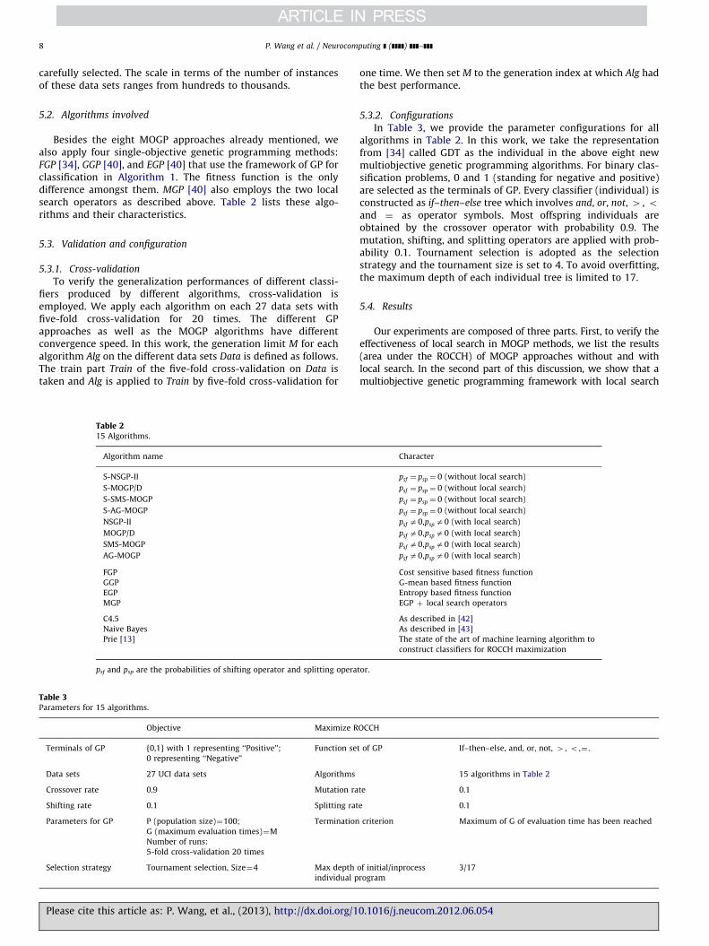
5.2. Algorithms involved

Besides the eight MOGP approaches already mentioned, wealso apply four single-objective genetic programming methods:FGP [34], GGP [40], and EGP [40] that use the framework of GP forclassification in Algorithm 1. The fitness function is the onlydifference amongst them. MGP [40] also employs the two localsearch operators as described above. Table 2 lists these algo-rithms and their characteristics.

5.3. Validation and configuration

5.3.1. Cross-validation

To verify the generalization performances of different classi-fiers produced by different algorithms, cross-validation isemployed. We apply each algorithm on each 27 data sets withfive-fold cross-validation for 20 times. The different GPapproaches as well as the MOGP algorithms have differentconvergence speed. In this work, the generation limit M for eachalgorithm Alg on the different data sets Data is defined as follows.The train part Train of the five-fold cross-validation on Data istaken and Alg is applied to Train by five-fold cross-validation for

Table 215 Algorithms.

Algorithm name

S-NSGP-II

S-MOGP/D

S-SMS-MOGP

S-AG-MOGP

NSGP-II

MOGP/D

SMS-MOGP

AG-MOGP

FGP

GGP

EGP

MGP

C4.5

Naive Bayes

Prie [13]

psf and psp are the probabilities of shifting operator and splitting opera

Table 3Parameters for 15 algorithms.

Objective Maximize R

Terminals of GP {0,1} with 1 representing ‘‘Positive’’; Function se

0 representing ‘‘Negative’’

Data sets 27 UCI data sets Algorithms

Crossover rate 0.9 Mutation ra

Shifting rate 0.1 Splitting rat

Parameters for GP P (population size)¼100; Termination

G (maximum evaluation times)¼M

Number of runs:

5-fold cross-validation 20 times

Selection strategy Tournament selection, Size¼4 Max depth

individual p


one time. We then set M to the generation index at which Alg hadthe best performance.

5.3.2. Configurations

In Table 3, we provide the parameter configurations for allalgorithms in Table 2. In this work, we take the representationfrom [34] called GDT as the individual in the above eight newmultiobjective genetic programming algorithms. For binary clas-sification problems, 0 and 1 (standing for negative and positive)are selected as the terminals of GP. Every classifier (individual) isconstructed as if–then–else tree which involves and, or, not, 4 , oand ¼ as operator symbols. Most offspring individuals areobtained by the crossover operator with probability 0.9. Themutation, shifting, and splitting operators are applied with prob-ability 0.1. Tournament selection is adopted as the selectionstrategy and the tournament size is set to 4. To avoid overfitting,the maximum depth of each individual tree is limited to 17.

5.4. Results

Our experiments are composed of three parts. First, to verify theeffectiveness of local search in MOGP methods, we list the results(area under the ROCCH) of MOGP approaches without and withlocal search. In the second part of this discussion, we show that amultiobjective genetic programming framework with local search

Character

psf ¼ psp ¼ 0 (without local search)




psf a0,psp a0 (with local search)




Cost sensitive based fitness function

G-mean based fitness function

Entropy based fitness function

EGP þ local search operators

As described in [42]

As described in [43]

The state of the art of machine learning algorithm to

construct classifiers for ROCCH maximization

tor.

OCCH

t of GP If–then–else, and, or, not, 4 , o ,¼ .

15 algorithms in Table 2

te 0.1

e 0.1

criterion Maximum of G of evaluation time has been reached

of initial/inprocess

rogram

3/17

0.1016/j.neucom.2012.06.054i





can work better than single-objective genetic programming withoutor with local search. Finally, traditional machine learning algorithmsare compared to MOGP with local search to certify the efficiency ofour algorithms in maximizing the ROC performance.

5.4.1. Results of MOGP without and with local search

Table 4 describes the performance of MOGP methods with andwithout local search on 27 UCI data sets. In the second column ofTable 4, the first sub-column shows the results of NSGP-II withoutlocal search (named S-NSGP-II) and the results of NSGP-II withlocal search (named NSGP-II) are shown in the second sub-column. A number is printed in bold face if the results arestatistically significantly better than the other variant of the samealgorithm according to the Wilcoxon sum-rank tests [44] with aconfidence level of 0.95. The results of MOGP/D, SMS-MOGP andAG-MOGP with and without local search are described in thethird, fourth, and fifth columns. The last row of Table 4 gives thenumber of wins, the number of draws, and the number of lossesfor all data sets.

From this table we can see that S-NSGP-II wins never, loses 22times to NSGP-II, and does not perform different in five of the 27UCI data sets. This means that the local search operator workswell and improves the performance of S-NSGP-II. Additionally,MOGP/D wins against S-MOGP/D on all data sets, SMS-MOGP andAG-MOGP lose only one time against their version without localsearch operators. Table 4 therefore testifies the effectiveness ofthe local search in MOGP approaches for maximizing the ROCperformance.

5.4.2. Results of single-objective GP and traditional machine

learning algorithms

In this subsection, we present all results of the four single-objective genetic programming algorithms [40] on 27 data sets. InTable 5, the first column gives the names of the data sets involvedand the second to the fifth column the results (mean and standarddeviation are multiplied by 100). The last four rows list the

Table 4Performance of MOGP methods without and with local search on UCI data sets, mean

Data set S-NSGP-II NSGP-II S-MOGP/D MOGP/D

australian 90.9372.52 92.0072.46 88.0975.37 91.6872bands 71.7175.43 77.7073.49 69.0574.47 76.4774bcw 98.1270.80 98.1970.99 97.7171.33 98.0771crx 90.1873.12 91.7972.47 89.5374.88 91.5872euthyroid 79.2779.20 96.7871.37 72.46710.39 94.4776german 73.0073.94 74.0372.81 68.0875.35 73.5272haberman 65.5576.60 67.0876.19 63.6877.17 66.6076hill-valley 50.3071.47 53.1972.61 50.0771.47 53.0272house-votes 97.0173.82 98.1071.39 96.5072.87 97.8471hypothyroid 79.63711.60 97.9971.52 77.41714.60 97.1172ionosphere 86.8176.76 91.8373.98 84.6176.73 91.4273kr-vs-kp 88.6777.32 98.0170.85 80.4178.04 98.1270mammographic 89.0872.05 89.7971.80 87.7172.52 89.4572monks-1 94.8073.43 99.9370.53 88.75711.39 99.4571monks-2 77.6579.50 93.6075.25 68.18710.74 89.8271monks-3 98.2274.26 100.0070.00 94.5179.50 99.8470mushroom 98.7071.61 99.9570.10 96.9373.15 99.7770parkinsons 85.0976.58 86.1775.96 80.8778.00 86.9675pima 77.2273.52 80.6173.21 72.5475.07 80.3572sonar 70.4276.01 80.0975.55 67.5177.43 79.6876spambase 70.9778.55 96.3670.57 64.1777.67 95.8070spect 75.4775.05 76.5276.91 73.9078.34 76.9777spectf 68.3075.95 73.3875.55 66.4378.58 73.5875tic-tac-toe 73.3978.99 86.19711.46 67.52711.04 84.1879transfusion 68.9774.89 72.1274.44 64.9474.75 71.8874wdbc 93.5274.95 97.2871.49 92.4274.73 97.0271wpbc 59.5278.15 67.4178.33 59.4277.76 66.6177

Win–draw–loss 0–5–22 22–5–0 0–0–27 27–0–0


outcomes of Wilcoxon rank-sum tests of all seven testedapproaches versus the four MOGP methods with local search. InTable 6, we list the outcomes of the Wilcoxon rank-sum testapplied to the results of single- and multi-objective geneticprogramming algorithms. As FGP and GGP have the same repre-sentation (GDT) with the MOGP methods without local search,the main different factor is the multi-objective strategy. At thesame time, the main difference between the MGP and MOGPmethods with local search is the multiobjective strategy. Fromthis table, it becomes obvious that multiobjective strategies ingenetic programming are able to improve the ROC performance inclassification problems.

As described in Table 5, the second to fifth columns report theresults of the four single-objective genetic programming algo-rithms on 27 data sets. From the sixth to the last column, we listthree traditional machine learning algorithms NB, C4.5, and PRIEwhich is the state of art in ROCCH maximization. In the last fourrows, the Wilcoxon rank-sum test is used to compare their resultswith those of the MOGP methods with local search. Taking21�6�0 as example, AG-MOGP wins 21 times, losses 0 time,and six times scores equal against EGP. Obviously, AG-MOGP isfar better than EGP in ROCCH maximization on the data sets weused. From the last four Wilcoxon rank-sum test results, it is clearthat multiobjective GP strategies with local search outperformsignificantly the four single-objective genetic programming algo-rithms and the three standard machine learning algorithms.

5.4.3. Analysis on MOGP for maximizing the ROC performance

Table 7 shows the Wilcoxon rank-sum test results among theMOGP methods with and without local search. Here, we use Fig. 8to illustrate the relationship of these four MOGP approaches withlocal search. The algorithm at the head of arrow is better than theone at the end of arrow, and the results show that NSGP-II is thebest algorithm among the tested ones. At the same time, MOGP/Dis slightly better than SMS-MOGP and AG-MOGP which have aroughly similar performance on all 27 data sets. Fig. 9 describes

and standard deviation, multiplied by 100, are given in this table.

S-SMS-MOGP SMS-MOGP S-AG-MOGP AG-MOGP

.44 89.1374.21 92.0272.33 90.3973.03 91.0579.49

.05 68.5174.28 75.5273.71 73.1274.91 77.0273.70

.13 97.0471.83 97.9571.14 97.9271.21 97.2579.87

.32 89.3474.56 91.6572.21 90.7173.09 90.8879.47

.91 75.05710.51 96.4971.32 80.1978.83 96.3477.45

.97 71.7574.23 73.6872.56 72.6473.51 73.1177.82

.58 65.0377.48 65.5077.12 66.8876.56 66.2779.44

.59 50.5871.37 52.6572.61 50.3071.32 52.4275.95

.46 96.9572.42 98.1371.23 97.7571.58 96.9479.89

.06 81.54712.99 97.7771.54 90.06711.45 98.13710.28

.56 84.8975.74 90.3775.02 87.4674.86 90.6779.97

.99 83.8076.48 98.2670.93 87.2077.35 97.1679.84

.00 88.1772.18 89.2371.84 89.1471.95 88.5579.11

.97 83.75712.99 97.9573.88 94.2075.97 97.48710.186.76 69.57710.18 85.4476.85 76.0179.69 82.80710.11.45 92.5279.99 98.6075.08 99.5270.49 98.7679.99

.30 97.0972.71 99.7970.36 98.5972.45 99.3573.07

.02 81.7672.32 85.8275.81 83.0876.22 84.78710.20

.86 75.2074.12 80.1173.07 77.9773.62 79.1678.54

.05 69.3477.97 79.3875.93 71.7476.48 78.0479.39

.60 64.8578.94 96.0470.63 93.3870.92 95.0279.61

.85 73.1977.39 76.0077.11 75.21 7 7.27 75.20710.19

.65 68.3877.47 75.2976.31 71.5276.52 74.9079.69

.06 69.12711.85 77.0674.28 71.31710.70 75.90712.95

.63 67.0475.45 71.94 72.58 68.4075.17 70.9878.43

.63 92.9173.95 97.0871.83 94.1473.08 96.2379.86

.41 61.0078.36 66.9278.88 60.9478.36 66.0479.85

0–1–26 26–1–0 0–6–21 21–6–0

0.1016/j.neucom.2012.06.054i




Table 6Wilcoxon rank-sum test results for MOGP methods without local search and single-objective genetic programming. FGP, EGP and four MOGP methods

without local search have the same representation. MGP and four local search-based MOGP approaches take shifting and splitting operators into their

search strategies.

Algorithms FGP GGP MGP

S-NSGP-II 26–0–1 20–5–1 NSGP-II 15–9–3

S-MOGP/D 25–1–1 16–6–5 MOGP/D 10–11–6

S-SMS-MOGP 26–0–1 18–6–3 SMS-MOGP 9–10–8

S-AG-MOGP 26–1–0 22–5–0 AG-MOGP 9–10–8

Table 5Performance of single-objective genetic programming and traditional machine learning algorithms on UCI data sets.

Data set EGP FGP GGP MGP NB Prie C4.5

australian 90.0573.06 85.5674.87 85.5473.83 90.667 2.68 89.477 2.78 91.757 2.36 85.527 4.05

bands 70.0475.05 53.9975.56 64.8874.89 76.1874.97 73.917 4.68 76.077 4.81 74.657 0.00

bcw 97.3571.37 93.7372.11 93.8572.45 97.237 1.52 98.927 0.62 98.167 1.09 95.0572.55

crx 90.6872.49 85.9173.57 86.3673.32 90.757 2.53 87.887 3.16 90.657 2.77 85.5170.00

euthyroid 93.3775.81 50.0170.11 79.41713.12 97.4771.41 91.917 2.03 96.247 1.31 92.9772.49

german 70.8173.42 51.7573.51 67.1475.36 71.697 3.30 78.427 2.94 75.957 3.25 65.3670.00

haberman 62.9777.63 50.6674.25 63.9876.68 64.1477.69 65.007 7.19 69.587 7.26 63.9670.00

hill-valley 50.1872.15 50.0971.39 49.9073.25 53.347 3.00 50.647 3.65 51.827 3.93 50.0070.00

house-votes 97.7571.63 94.6374.00 95.2373.85 97.747 1.62 98.057 1.04 97.807 1.49 96.3572.04

hypothyroid 96.5572.55 52.3573.27 93.4575.91 98.197 1.77 98.027 1.52 96.517 2.45 95.5673.23

ionosphere 87.2275.84 80.8777.60 79.8677.01 90.097 4.76 93.577 3.18 93.687 4.23 88.2075.65

kr-vs-kp 85.7176.65 62.1678.52 71.8976.02 98.447 1.06 93.217 1.00 98.267 0.44 99.7170.23

mammographic 88.9671.97 82.7673.60 84.7373.46 88.687 2.24 89.777 1.96 89.707 2.02 87.6670.00

monks-1 85.96711.96 51.2179.96 75.0375.25 99.647 1.66 73.187 4.58 70.937 5.59 75.2270.00

monks-2 80.48712.05 50.0176.29 53.2876.92 94.767 4.88 52.387 7.04 51.257 6.16 94.1775.93

monks-3 99.5970.49 87.48710.72 86.7579.04 99.907 0.29 95.947 2.17 99.607 0.27 100.0070.00

mushroom 98.6871.88 84.6778.24 89.4474.47 99.957 0.13 92.607 0.71 99.497 0.14 100.0070.00

parkinsons 81.9277.80 76.6278.22 75.9777.19 85.877 7.20 85.917 6.11 88.247 5.83 78.9179.76

pima 76.2774.94 50.8871.29 70.7373.44 78.777 3.71 81.407 3.01 79.587 2.92 75.2374.93

sonar 73.3377.01 54.1776.81 68.2277.38 77.597 7.57 80.127 7.03 69.927 8.64 73.8577.84

spambase 85.2875.53 76.1477.16 76.5874.30 94.797 1.04 93.987 0.69 96.727 0.56 93.7270.00

spect 74.3677.01 68.21710.68 71.9977.18 75.337 8.59 84.097 6.03 83.517 7.01 76.8878.91

spectf 71.7677.04 58.6979.06 69.1677.16 73.107 8.45 84.947 5.19 78.907 6.37 63.3679.07

tic-tac-toe 71.89712.11 63.3579.73 63.35710.15 90.047 10.24 61.527 14.76 70.417 12.51 84.91713.91

transfusion 71.3175.21 50.4870.89 67.4674.37 71.317 4.88 70.937 4.94 70.877 5.39 71.0875.08

wdbc 95.1272.92 87.2574.54 90.3972.83 96.057 1.92 98.147 1.33 96.587 1.94 92.7473.16

wpbc 66.8379.90 56.4777.41 60.1578.92 64.217 10.66 66.427 8.85 68.227 9.25 58.19710.77

NSGP-II 23–4–0 27–0–0 27–0–0 15–9–3 13–8–6 13–7–7 20–5–2

MOGP/D 22–5–0 27–0–0 27–0–0 10–11–6 12–8–7 9–11–7 20–2–5

SMS-MOGP 21–6–0 27–0–0 27–0–0 9–10–8 12–8–7 9–11–7 20–2–5

AG-MOGP 21–6–0 27–0–0 26–1–0 9–10–8 14–6–7 11–9–7 20–2–5

Table 7Wilcoxon rank-sum test results for MOGP methods with and without local search.

Algorithms NSGP-II MOGP/D SMS-MOGP AG-MOGP

NSGP-II – 9–18–0 9–16–2 6–20–1

MOGP/D 0–18–9 – 3–20–4 4–20–3

SMS-MOGP 2–16–9 3–20–4 – 2–23–2

AG-MOGP 1–20–6 3–20–4 2–23–2 –

Algorithms S-AGE-MOGP S-MOGP/D S-SMS-MOGP S-NSGP-II

S-AG-MOGP – 22–5–0 19–8–0 5–20–2

S-MOGP/D 0–5–22 – 3–18–6 0–8–19

S-SMS-MOGP 0–8–19 6–18–3 – 0–9–18

S-NSGP-II 2–20–5 19–8–0 18–9–0 –


the relationship of these MOGP approaches without local search.Here, S-AG-MOGP is the best algorithms among four methods andit is slightly better than S-NSGP-II which is quite a lot better thanS-SMS-MOGP. S-MOGP/D is the worst algorithm. First of all, itshould be emphasized that NSGP-II is the best algorithm of allapproaches, with and without local search.

There are two factors affecting the performance of the testedalgorithms, one is the different ranking mechanisms used inmultiobjective optimization algorithms, the other is that the local


search operators have different efficacy when they are introducedinto different EMOAs. Comparing Fig. 9 with Fig. 8, we can findthat NSGP-II and MOGP/D are improved to the first and thesecond place. This means local search operators work well inmultiobjective optimization frameworks of NSGA-II and MOEA/D,and not as good in SMS-EMOA and AG-EMOA.

More evidence can be found in Table 10, which shows the totaltime cost in seconds of all MOGP methods and the difference ofthe approaches with and without local search. Local search

0.1016/j.neucom.2012.06.054i





operators seem to consume more time in MOGP/D framework andthe second longest time in NSGP-II framework. There are no hugedifferences of time cost in the SMS-MOGP and AG-MOGP frame-works. The reason for this is that the SMS-MOGP and AG-MOGPframeworks are very greedy strategies. As outline in Section 4.2.1,the contribution of each individual to their target metrics (hyper-volume or approximate distance) is directly used into selectmechanism. Additionally, the hypervolume is similar to the areaunder the ROCCH and minimizing the approximated distance isalso very similar to maximizing the hypervolume. As SMS-MOGPand AG-MOGP are greedy at searching the maximum ROCCH, itbecomes harder to escape a local optimum since the shifting andsplitting operators only perform exploitation. Hence, these twooperators cannot contribute much to SMS-MOGP and AG-MOGP.

NSGP-II, on the other hand, ranks the individuals by dom-inance level and crowding-distance and MOGP/D just comparesindividuals with others in their neighborhood. Both algorithmsare not very greedy at selecting individuals to survive and thesurvivors can potentially be improved by the local search opera-tors. From another perspective, SMS-MOGP and AG-MOGP have

Fig. 8. Comparisons among MOGP methods with local search.

Fig. 9. Comparisons among MOGP

Table 8Time cost of MOGP algorithms in seconds.

Time (s) S-NSGP-II S-MOGP/D S-SMS-MOGP S-A

australian 30.34 5.31 42.71 2

bands 81.84 122.68 24.55 10

bcw 4.96 5.51 9.82 1

crx 83.69 131.33 197.94 30

euthyroid 154.83 22.46 238.75 31

german 64.98 46 62.84 5

haberman 5.22 5.25 26.20

hill-valley 274.38 170.05 339.33 37

house-votes 6.86 1.79 91.90 18

hypothyroid 607.35 1376.31 799.97 6

ionosphere 12.07 3.98 16.32 2

kr-vs-kp 293.09 127.52 301.78 31

mammographic 15.22 11.92 24.44 3

monks-1 29.23 27.64 37.54 4

monks-2 134.2 121.59 138.32 14

monks-3 1.1 3.81 159.33 42

mushroom 857.63 698.38 682.44 49

parkinsons 1.55 1.09 1.96

pima 25.75 4.77 22.46 1

sonar 2.76 2.34 5.94

spambase 134.62 103.62 1189.80 285

spect 7.71 2.53 13.40 1

spectf 1.1 1.08 3.33

tic-tac-toe 84.52 81.51 96.32 9

transfusion 4.71 4.36 4.52

wdbc 4.79 1.89 4.88

wpbc 0.7 3.84 1.20

Sum time 2925.20 3088.56 4538.00 595


larger selection pressure than NSGP-II and MOGP/D in searchinggenetic decision trees to maximize the ROC performance.

The reason for why NSGP-II is better than MOGP/D is thediscordancy of the genotype and phenotype of genetic program-ming: two genetic programming individuals can be very similar indecision space, but may have a very long distance in objectivespace. In MOGP/D, an offspring is produced by two parents in aneighborhood which is defined in the objective space, but it willnot be in this neighborhood. This causes the framework of MOEA/D to not work well because it supposes that subproblems can beoptimized by individuals in their neighborhood.

5.4.4. Time cost of all algorithms

Tables 8 and 9 report the time cost of all algorithms. Theexperiment environment is an 8 core CPU with 2.13 GHz and24 GB RAM. Obviously, GP-based algorithms need much moretime than traditional machine learning algorithms. Because of themetaheuristic character of EAs, GP needs to evaluate manyclassifiers until it converges. The Naive Bayes method, on theother hand, calculates an a posteriori probability and the C4.5adopts uses a greedy method to increase information gain. PRIEemploys a greedy strategy to construct classifiers (more than one,usually dozens of classifiers) to maximize the ROCCH, so it costa little more time than NB and C4.5, but still much less thanGP-based algorithms.

Among the single-objective GP algorithms, MGP costs muchmore time than the others (EGP, FGP, GGP). The reason is thatlocal search operators exploit each individual. For the samereason, MOGP methods with local search will consume moretime than their counterparts without local search.

methods without local search.

G-MOGP NSGP-II MOGP/D SMS-MOGP AG-MOGP

8.12 51.65 31.18 22.88 48.74

9.3 70.65 117.45 24.25 122.61

1.69 3.06 7.24 5.03 15.66

0.69 82.38 87.43 82.81 155.47

3.61 806.02 529.17 159.92 214

8.48 258.99 274.96 76.43 67.62

9.98 3.82 3.88 5.04 4.13

8.59 971.96 1204.87 606.45 543.85

9.56 3.85 18.23 4.29 35.59

5.32 52.5 484.17 487.80 1569.87

0.74 28.5 19.28 8.96 82.59

2.55 159.18 882.05 304.78 334.64

3.58 34.95 98.57 17.74 104.11

5.6 21.86 19.64 15.80 28.09

2.11 318.01 489.36 162.39 208.77

1.66 27.57 43.82 3.98 7.98

1.46 607.59 718.55 662.13 805.04

2.44 2.2 2.22 2.71 1.44

8.16 51.64 74.73 25.50 54.3

9.06 7.92 24.69 6.61 6.36

6.4 2910.43 3509.06 1711.28 1520.9

4.79 32.66 21.06 6.29 6.99

5.81 2.12 1.97 6.79 10.33

8.32 699.82 399.07 156.73 109.5

4.69 36.69 41.49 7.05 4.67

6.45 7.14 5.78 7.04 9.81

1.68 2.5 4.33 1.54 1.88

0.84 7255.66 9114.25 4582.20 6074.94

0.1016/j.neucom.2012.06.054i




Table 9Time cost of single-objective genetic programming and machine learning algorithms.

Time(s) EGP FGP GGP MGP NB Prie C4.5 Time (s) EGP FGP GGP MGP NB Prie C4.5

australian 5.50 2.75 2.88 2.90 0.05 4.18 0.03 bands 5.50 2.50 2.70 121.26 0.09 15.85 0.08

bcw 10.93 13.55 13.14 6.77 0.03 0.53 0.01 crx 11.95 4.21 3.18 6.10 0.05 2.92 0.03

euthyroid 212.36 8.35 14.05 198.61 0.48 2.74 0.34 german 24.13 4.25 5.67 16.95 0.12 4.79 0.13

haberman 10.70 3.20 2.78 1.54 0.01 0.43 0.00 hill-valley 29.59 9.41 7.11 1507.34 0.42 380.82 0.08

house-votes 2.83 3.04 5.51 1.37 0.04 0.48 0.01 hypothyroid 79.04 47.37 48.36 45.38 0.50 3.20 0.20

ionosphere 20.76 142.17 13.91 15.67 0.05 5.77 0.04 kr-vs-kp 419.03 30.57 23.84 554.33 0.65 1.58 0.31

mammographic 20.74 7.64 5.00 46.07 0.03 0.87 0.02 monks-1 5.93 1.51 2.16 16.27 0.02 0.29 0.00

monks-2 200.47 20.76 14.98 59.35 0.01 0.30 0.01 monks-3 8.49 7.10 6.11 5.40 0.01 0.31 0.01

mushroom 1107.35 664.66 531.60 903.85 1.01 2.31 0.57 parkinsons 4.52 1.52 1.77 5.42 0.02 1.62 0.01

pima 30.50 20.73 12.10 20.81 0.03 16.46 0.02 sonar 5.90 5.77 5.56 10.12 0.05 31.45 0.03

spambase 90.32 65.99 16.67 2313.91 1.14 374.98 1.80 spect 4.92 2.91 1.04 9.35 0.03 0.39 0.02

spectf 9.71 8.76 2.88 8.62 0.05 3.81 0.03 tic-tac-toe 218.47 164.91 9.86 102.80 0.04 0.48 0.03

transfusion 33.79 93.27 3.48 6.71 0.02 4.34 0.01 wdbc 15.23 9.57 5.47 8.74 0.08 20.86 0.04

wpbc 7.77 1.96 1.36 3.04 0.02 7.89 0.04

Table 10Total time cost of local search operator in different MOGP methods.

Algorithms Time cost Time cost Difference

S-AG-MOGP 5950.84 AG-MOGP 6074.94 124.10

S-MOGP/D 3088.56 MOGP/D 9114.25 6025.69

S-SMS-MOGP 4538.00 SMS-MOGP/D 4582.20 44.20

S-NSGP-II 2925.20 NSGP-II 7255.66 4330.46


6. Conclusion and future work

In this work, we first pointed out that ROCCH is very suitableto measure the ROC performance in binary classification, espe-cially for especially if the class distribution is unknown or themisclassification cost are skew. Then, we discussed the relation-ship between ROCCH and the Pareto front in multiobjectiveoptimization: both can be considered as analogous to each other.

Maximizing the ROCCH can be archived by using evolutionarymultiobjective algorithms to search a group of nondominated solu-tions. Four different MO frameworks for synthesizing genetic decisiontrees are proposed: S-NSGP-II, S-MOGP/D, S-SMS-MOGP, and S-AG-MOGP, each employing a different fitness measure. We then pro-posed to use local search in genetic programming for classificationproblems. Two different local search operators called shifting andsplitting are defined. They are introduced into the MOGP methods toimprove the performance in searching Pareto front.

We found that these operators contribute differently in thedifferent MOGP methods. NSGP-II with local search outperformsthe other the MOGP algorithms both with and without localsearch. We furthermore compare the new approaches to single-objective genetic programming algorithms and traditionally


machine learning algorithms and found that they perform veryfavorable. In conclusion, NSGP-II with local search is the bestoverall algorithms for ROCCH maximization.

As pointed out in Section 3.2, ROCCH is not the same as thePareto front in multiobjective optimization. In this work, MOGPapproaches are adopted to search a group of nondominated geneticdecision trees to approximate the ROCCH and to maximize the areaunder the curve constructed by these nondominated solutions. Ourplan for future work is to combine the concepts of ROCCH andPareto front in a better way in order to derive new multiobjectiveevolutionary algorithms for maximizing the ROC performance.

In Section 5.4.1, we found that the contribution of the localsearch methods to improve the final results strongly depends on theMO framework. Therefore, further research should pay attention onhow local search operators work in multiobjective scenarios. Gen-erally, the concepts of memetic computing should be investigatedmore thoroughly in this domain, as they seemingly can lead tosignificant improvements in ROCCH maximization problems.

The last issue we want to tackle is the dissatisfying runtime ofour methods. This is a disadvantage for EAs in general, but may bemitigated by using parallelization and new hardware such as GPUs.

Acknowledgment

This work was partially supported by the 973 Program ofChina (Grant no. 2011CB707006), National Natural Science Foun-dation of China (Grant nos. U0835002, 61028009 and 61175065),the National Natural Science Foundation of Anhui Province (No.1108085J16), and the European Union Seventh Framework Pro-gramme under Grant agreements no. 247619.

Appendix A. MOGP algorithms

Algorithm 2. fast-nondominated-sort(P) [30].

Require: Panull

1:
P is a solution set Ensure: fast-nondominated-sort 2: for each pAP do 3: Sp ¼ |
4:
np¼0 5: for each qAP do 6: if p!q then 7: Sp ¼ Sp [ fqg
0.1016/j.neucom.2012.06.054i





8:

Please c

else fq!pg

9:
np ¼ npþ1
10:
end if 11: end for 12: if np¼0 then 13: Prank ¼ 1 14: F1 ¼ F1 [ fpg
15:
end if 16: end for 17: while Fia| do 18: Q ¼ | 19: for each pAFi do 20: for each qASp do
21:
nq ¼ nq�1
22:
if nq¼0 then 23: qrank ¼ iþ1 24: Q ¼Q [ fqg
25:
end if 26: end for 27: end for 28: i¼ iþ1 29: Fi ¼Q
30:
end while
Algorithm 3. crowding-distance-assignment (T) [30].

Require: Tanull

1:
T is a nondominated solution set Ensure crowding-distance-assignment 2: l¼ 9T9 3: for each iA ½1,l� do 4: T½i�distance ¼ 0 5: end for 6: for each objective m do 7: T ¼ sortðT ,mÞ 8: T½1�distance ¼ T½l�distance ¼1
9:
for i¼2 to l�1 do 10: T½i�distance ¼ T½i�distanceþðT½iþ1�:m�T½i�1�:mÞ=ðf max
m �f minm Þ

11:
end for 12: end for
Algorithm 4. NSGP-II(P,Max,N).

i

Require: MaxZ03P¼ null3N40
1: Max is the maximum9evaluations
2:
P is the population 3: N is the population size Ensure: NSGA-II 4: Let m¼ 0,t¼ 0 5: Initialize the population Pt by ramped-half-and-half method
6:
Evaluate each individual in Pt and m¼mþN
7:
while mrMax do 8: Generate offspring Qt from Pt by tree-based crossover
9:
Shifting operator with probability psf
10:
Splitting operator with probability psp
11:
Evaluate each changed offspring in Qt
12:
m¼mþ9 changed-offspring 9 13: Rt ¼ Pt [ Qt
14:
F¼fast- nondominated-sort ðRtÞ
15:
Ptþ1 ¼ | and i¼0 16: while 9Ptþ19þ9Fi9rN do
17:
crowding-distance-assignment(Fi) 18: Ptþ1 ¼ Ptþ1 [ Fi
19:
i¼ iþ1
te this article as: P. Wang, et al., (2013), http://dx.doi.org/10.1016/j.neucom.2012.06.054i





20:

Please ci

end while
21: Sort(Fi, !n) 22: Ptþ1 ¼ Ptþ1 [ Fi½1 : ðN�9Ptþ19Þ� 23: P¼ Ptþ1
24:
t¼ tþ1 25: end while 26: Return P
Algorithm 5. MOGP/D(EP,P,N,M,T).

Require: EP¼ null3N403MZ23T40
1: EP(External Population) is an archive to collect pareto-optimal solutions 2: P is the population contains N solutions ðx1, . . . ,xNÞ where xi is the current solution for the ith subproblem 3: N is the population size and is also the number of subproblems in MOEA/D 4: M is the number of objectives 5: A uniform spread of N weight vectors: l1, . . . ,lN ,li
¼ ðli1, . . . ,li

MÞ for 1r irN

6:
T is the number of weight vectors in the neighborhood of each weight vector 7: Reference point zn
8:
FV ðkÞ is the F-value of xi 1r irN
Ensure: MOGP/D
9: Step 1) Initialization 10: Step 1.1) Set EP¼ | 11: Step 1.2) Compute the Euclidean distances between any two weight vectors and then work out the T closest weight vectors to
each weight vector. For each i¼ 1, . . . ,N, Set BðiÞ ¼ i1, . . . ,iT , where li1 , . . . ,liT are the T closest weight vectors to li

12:
Step 1.3) Generate an initial population ðx1, . . . xNÞby ramped-half-and-half method
13:
Step 2) Update 14: for i¼ 1, . . . ,N do 15: Step 2.1) Reproduction: Randomly select two indexes k,l for B(i), and then generate a new solution y by xk and xl by using tree-
based crossover operators
16: Step 2.2) Improvement: Apply shifting operator probability psf and splitting operator with probability psp on y to produce y0
17:
Step 2.3) Update of neighboring solutions: For each index jABðiÞ, if gteðy09lj,znÞrgteðxj9lj,znÞ, then set xj ¼ y0 and FVj¼ Fðy0Þ
18:
Step 2.4) Update of EP
19:
Remove from EP all the vectors dominated by FðyiÞ
20:
Add FV 0 to EP if no vectors in EP dominate FðyiÞ
21:
end for 22: Step 3) Stopping Criteria: If stopping criteria is satisfied then stop and output EP. Otherwise, go to Step 2
Algorithm 6. Reduce (Q) [36].

Require: Q a|
1: Q is a solution set Ensure: Reduce 2: R1, . . . ,Rv’fast-nondominated-sortðQ Þ
3:
if v41 then 4: r’argmaxsARv
½dðs,Q Þ�

5:
else 6: r’argminsARv
½DBðs,RvÞ�

7:
end if 8: Return (Q frg)
Algorithm 7. SMS-MOGP (Max,N).

Require: Max40,N40
1: Max is the maximum of evaluations 2: N is the population size Ensure: SMS-MOGP 3: P0 ¼ initðÞ by ramped-half-and-half method
4:
t¼0 5: m¼0 6: while moMax do 7: qtþ1’Shifting operator with probability psf
splitting operator with probability psp are done on Pt

8:
Ptþ1’ReduceðPt [ qtþ1Þ
te this article as: P. Wang, et al., (2013), http://dx.doi.org/10.1016/j.neucom.2012.06.054i





9:

Please ci

t’tþ1
10: m’mþ1 11: end while
Algorithm 8. MeasureQuality(A,P) [33].

Require: Aa|3Pa|
1: A Archive 2: P Population Ensure: MeasureQuality 3: S’| 4: for each aAA do 5: d’1 6: for each pAP do 7: r’�1 8: for i’d do 9: r’maxfr,ai�pig
10:
end for 11: d’minfd,rg 12: end for 13: S’S [ d 14: end for 15: sort S decreasingly 16: Return S
Algorithm 9. AG-MOGP(Max,A,P, m, l).

Require: A¼ |3P¼ |3Max403m403l40
1: A Archive 2: P Population 3: Max is the maximum of evaluations 4: m and l are the size of parent and offspring population Ensure AGEMOA 5: Initialize population P with m by ramped-half-and-half method
6:
Set archive A’P, m’0 7: while moMax do 8: Initialize offspring population O’| 9: for j’1 to l do 10: Select two random individuals from P
11:
Apply crossover operator 12: Shifting operator with probability psf
13:
Splitting operator with probability psp
14:
Add new individual into O
15:
end for 16: for each pAO do 17: Insert offspring p in archive A
18:
end for 19: Add offsprings to population, i.e., P’P [ O
20:
while 9P94m do
21:
for each pAP do 22: MeasureQuality(A, P\fpg) 23: end for 24: Remove p from P for which SaðA,P\fpgÞ is lexicographically smallest 25: end while 26: end while
References

[1] T. Fawcett, An introduction to roc analysis, Pattern Recogn. Lett. 27 (8) (2006)861–874.

[2] C.M. Bishop, Pattern Recognition and Machine Learning, Springer-VerlagGmbH, Berlin, Germany, 2006.

[3] F. Provost, T. Fawcett, Analysis and visualization of classifier performance:comparison under imprecise class and cost distributions, in: Proceedings of

te this article as: P. Wang, et al., (2013), http://dx.doi.org/1

the Third International Conference on Knowledge Discovery and Data Mining,Amer Assn for Artificial, 1997, pp. 43–48.

[4] J. Egan, Signal Detection Theory and ROC Analysis, Series in Cognition andPerception, Academic Press, 1975.

[5] H. Sox, M. Higgins, Medical Decision Making, Amer College of Physicians, 1988.[6] A. Bradley, The use of the area under the roc curve in the evaluation of

machine learning algorithms, Pattern Recognition 30 (7) (1997) 1145–1159.[7] F. Provost, T. Fawcett, Robust classification for imprecise environments,

Mach. Learn. 42 (3) (2001) 203–231.

0.1016/j.neucom.2012.06.054i





[8] T. Fawcett, Using rule sets to maximize roc performance, in: Proceedings IEEEInternational Conference on Data Mining, 2001. ICDM 2001, IEEE, pp. 131–138.

[9] P. Flach, S. Wu, Repairing concavities in roc curves, in: Proceedings of the19th International Joint Conference on Artificial Intelligence (IJCAI05), 2005,pp. 702–707.

[10] R. Prati, P. Flach, Roccer: an algorithm for rule learning based on roc analysis,in: Proceedings of the 19th International Joint Conference on ArtificialIntelligence, Morgan Kaufmann Publishers Inc., 2005, pp. 823–828.

[11] M. Barreno, A.A. Cardenas, J.D. Tygar, Optimal roc curve for a combination ofclassifiers, Adv. Neural Inf. Process. Syst. 20 (X) (2008) 57–64.

[12] L. Cam, Neyman–Pearson Lemma, Encyclopedia of Biostatistics.[13] T. Fawcett, Prie: a system for generating rule lists to maximize roc

performance, Data Min. Knowl. Discov. 17 (2) (2008) 207–224.[14] J. Koza, Genetic Programming: On the Programming of Computers by Means

of Natural Selection, The MIT Press, 1992.[15] R. Poli, W. Langdon, N. McPhee, A Field Guide to Genetic Programming, Lulu

Enterprises UK Ltd, 2008.[16] P. Espejo, S. Ventura, F. Herrera, A survey on the application of genetic

programming to classification, IEEE Trans. Syst. Man Cybernet. Part C: Appl.Rev. 40 (2) (2010) 121–144.

[17] P. Wang, T. Weise, R. Chiong, Novel evolutionary algorithms for supervisedclassification problems: an experimental study, Evolut. Intell. 4 (1) (2011)3–16, http://dx.doi.org/10.1007/s12065-010-0047-7.

[18] W. Tackett, Genetic programming for feature discovery and image discrimi-nation, in: Proceedings of the Fifth International Conference on GeneticAlgorithms, ICGA-93, Citeseer, 1993, pp. 303–309.

[19] J. Li, X. Li, X. Yao, Cost-sensitive classification with genetic programming, in:2005 IEEE Congress on Evolutionary Computation (CEC), IEEE, 2005,pp. 2114–2121.

[20] Y. Zhang, H. Li, M. Niranjan, P. Rockett, Applying cost-sensitive multiobjectivegenetic programming to feature extraction for spam e-mail filtering, GeneticProgram. (2008) 325–336.

[21] E. Alfaro-Cid, K. Sharman, A. Esparcia-Alcazar, A genetic programmingapproach for bankruptcy prediction using a highly unbalanced database, AI2007: Appl. Evolut. Comput. (2007) 169–178.

[22] G. Patterson, M. Zhang, Fitness functions in genetic programming for classifica-tion with unbalanced data, AI 2007: Adv. Artif. Intell. (2007) 769–775.

[23] U. Bhowan, M. Johnston, M. Zhang, X. Yao, Evolving diverse ensembles usinggenetic programming for classification with unbalanced data, IEEE Trans.Evolut. Comput, http://dx.doi.org/10.1109/TEVC.2012.2199119, in press.

[24] P. Flach, Roc Analysis, Encyclopedia of Machine Learning, Springer, Berlin,Heidelberg, 2010, pp. 869–874.

[25] G. Hughes, On the mean accuracy of statistical pattern recognizers, IEEETrans. Inf. Theory 14 (1) (1968) 55–63.

[26] K. Spackman, Signal detection theory: valuable tools for evaluating inductivelearning, in: Proceedings of the Sixth International Workshop on MachineLearning, Morgan Kaufmann Publishers Inc., 1989, pp. 160–163.

[27] M. Scott, M. Niranjan, R. Prager, Realisable classifiers: improving operatingperformance on variable cost problems, in: Proceedings of the Ninth BritishMachine Vision Conference, vol. 1, Citeseer, 1998, pp. 304–315.

[28] H. Li, Q. Zhang, Multiobjective optimization problems with complicated paretosets, moea/d and nsga-ii, IEEE Trans. Evolut. Comput. 13 (2) (2009) 284–302.

[29] T. Weise, Global Optimization Theory and Application, it-weise.de (Self-Pub-lished), Germany, 2009. URL /http://www.it-weise.de/projects/book.pdfS.

[30] K. Deb, A. Pratab, S. Agrawal, T. Meyarivan, A fast and elitist multiobjectivegenetic algorithm: NSGA-II, IEEE Trans. Evolut. Comput. (IEEE-EC) 6 (2)(2002) 182–197.

[31] Q. Zhang, H. Li, Moea/d: a multiobjective evolutionary algorithm based ondecomposition, IEEE Trans. Evolut. Comput. 11 (6) (2007) 712–731.

[32] E. Zitzler, L. Thiele, Multiobjective evolutionary algorithms: a comparativecase study and the strength pareto approach, IEEE Trans. Evolut. Comput. 3(4) (1999) 257–271.

[33] K. Bringmann, T. Friedrich, F. Neumann, M. Wagner, Approximation-guidedevolutionary multi-objective optimization, in: Proceeding of the 22nd Inter-national Joint Conference on Artificial Intelligence, Barcelona, Spain, 2011,pp. 1198–1203.

[34] L. Jin, FGP: A Genetic Programming Based Financial Forecasting Tool, Ph.D.Thesis, Citeseer, 2000.

[35] J. Backus, The syntax and semantics of the proposed international algebraiclanguage of the Zurich acm-gamm conference, in: Proceedings of theInternational Conference on Information Processing, 1959.

[36] N. Beume, B. Naujoks, M. Emmerich, Sms-emoa: multiobjective selection basedon dominated hypervolume, Eur. J. Operat. Res. 181 (3) (2007) 1653–1669.

[37] E. Zitzler, L. Thiele, An Evolutionary Algorithm for Multiobjective Optimization:The Strength Pareto Approach, TIK-Report 43, Eidgenossische TechnischeHochschule (ETH) Zurich, Department of Electrical Engineering, ComputerEngineering and Networks Laboratory (TIK), Zurich, Switzerland, May 1998.

[38] E. Zitzler, M. Laumanns, L. Thiele, SPEA2: Improving the Strength ParetoEvolutionary Algorithm, TIK-Report 101, Eidgenossische TechnischeHochschule (ETH) Zurich, Department of Electrical Engineering, ComputerEngineering and Networks Laboratory (TIK), Zurich, Switzerland, ErrataAdded 2001-9-27, May 2001.

[39] T. Weise, R. Chiong, K. Tang, Evolutionary optimization: pitfalls and boobytraps, J. Comput. Sci. Technol. 27 (5) (2012) 907–936.

[40] P. Wang, K. Tang, E.P.K. Tsang, X. Yao, A memetic genetic programming withdecision tree-based local search for classification problems, in: Proceedings


of the 12th IEEE Congress on Evolutionary Computation (CEC’11), 2011,pp. 917–924. http://dx.doi.org/10.1109/CEC.2011.5949716.

[41] UCI, Uc Irvine Machine Learning Repository, 2009. URL /http://archive.ics.uci.edu.c/mlS.

[42] J. Quinlan, C4.5: Programs for Machine Learning, Morgan, Kaufmann, 1993.[43] I. Rish, An empirical study of the Naive Bayes classifier, in: IJCAI 2001 Workshop

on Empirical Methods in Artificial Intelligence, vol. 3, 2001, pp. 41–46.[44] F. Wilcoxon, Individual comparisons by ranking methods, Biomet. Bull. 1 (6)

(1945) 80–83.

Pu Wang received the bachelors degree in computerscience from the University of Science and Technologyof China (USTC), Hefei, China, in 2008. He is currentlypursuing the PhD degree from the Nature InspiredComputation and Applications Laboratory (NICAL),School of Computer Science and Technology, USTC.

His current research interests include evolutionarycomputation, memetic algorithms, and multiobjectiveoptimization for classification problems in machinelearning, and genetic programming for model checkingin software engineering.

Ke Tang received the BEng degree from the HuazhongUniversity of Science and Technology, Wuhan, China,in 2002, and the PhD degree from the School ofElectrical and Electronic Engineering, Nanyang Tech-nological University, Singapore, in 2007. In 2007, hejoined the Nature Inspired Computation and Applica-tions Laboratory (NICAL), School of Computer Scienceand Technology, University of Science and Technologyof China, Hefei, China, as an Associate Professor, andwas promoted to Professor in 2011. He is also anHonorary Senior Research Fellow in the School ofComputer Science, University of Birmingham, UK. He
has authored/co-authored more than 50 refereed pub-
lications. His major research interests include evolutionary computation, machinelearning, meta-heuristic algorithms, and real-world applications. He is an Associ-ate Editor of IEEE Computational Intelligence Magazine and served as a programco-chair of CEC2010, held in Barcelona.

Thomas Weise received the Diplom Informatiker(equivalent to MS) degree from the Department ofComputer Science, Chemnitz University of Technology,Chemnitz, Germany, in 2005, and the PhD degree fromthe Distributed Systems Group of the FachbereichElektrotechnik and Informatik, University of Kassel,Kassel, Germany, in 2009.

Since 2009, he has been a Researcher with theNature Inspired Computation and Applications Labora-tory, School of Computer Science and Technology,University of Science and Technology of China, Hefei,Anhui, China. He has been an Associate Professor in
USTC since 2011. His experience ranges from applying
genetic programming to distributed systems and multiagent systems, efficientweb service composition for service oriented architectures, to solving large-scalereal-world vehicle routing problems for multimodal logistics and transportation.Besides being the author and co-author of over 40 refereed publications, he alsoauthors the electronic book Global Optimization Algorithms—Theory and Applica-tion which is freely available at his website http://www.itweise.de. His majorresearch interests include evolutionary computation, genetic programming, andreal-world applications of optimization algorithms.

Edward Tsang received the bachelor degree in busi-ness administration from the Chinese University ofHong Kong, Shatin, Hong Kong, in 1977, and the MScand PhD degrees in computer science from the Uni-versity of Essex, Colchester, UK, in 1983 and 1987,respectively. He is currently a Professor in ComputerScience at the School of Computer Science and Elec-tronic Engineering, University of Essex, Colchester, UK,where he is also the Co-Founder and the Director ofthe Center for Computational Finance and EconomicAgents, an interdisciplinary research center. He waswith companies including British Telecom, London,
UK, Honda Europe, Ghent, Belgium, and OANDA, NY.
Main techniques used in his research include heuristic search, optimization, andevolutionary computation. With background and experience in industry, he has

0.1016/j.neucom.2012.06.054i

http://dx.doi.org/10.1007/s12065-010-0047-7

http://dx.doi.org/10.1007/s12065-010-0047-7

http://dx.doi.org/10.1007/s12065-010-0047-7

dx.doi.org/10.1109/TEVC.2012.2199119

http://www.it-weise.de/projects/book.pdf

dx.doi.org/http://dx.doi.org/10.1109/CEC.2011.5949716

http://archive.ics.uci.edu.c/ml

http://archive.ics.uci.edu.c/ml

http://www.itweise.de





broad interest in business applications of artificial intelligence, including compu-tational finance, computational economics, and constraint satisfaction.

He was the Founding Chair of the IEEE Computational Finance and EconomicsTechnical Committee in which he is an Active Member.

Xin Yao received the BSc degree from the University ofScience and Technology of China (USTC), Hefei, China,in 1982, the MSc degree from the North China Instituteof Computing Technology, Beijing, China, in 1985, andthe PhD degree from USTC in 1990.

From 1985 to 1990, he was an Associate Lecturerand Lecturer with USTC, while working toward thePhD degree in simulated annealing and evolutionaryalgorithms. In 1990, he was a Postdoctoral Fellow withthe Computer Sciences Laboratory, Australian NationalUniversity, Canberra, Australia, where he continued hiswork on simulated annealing and evolutionary algo-
rithms. In 1991, he was with the Knowledge-Based
Systems Group, Commonwealth Scientific and Industrial Research Organization,Division of Building, Construction and Engineering, Melbourne, Australia, wherehe worked primarily on an industrial project on automatic inspection of sewage


pipes. In 1992, he returned to Canberra to take up a lectureship in the School ofComputer Science, University College, University of New South Wales, AustralianDefense Force Academy, Sydney, Australia, where he was later promoted to aSenior Lecturer and Associate Professor. Since April 1999, he has been a Professor(Chair) of computer science in the University of Birmingham, Birmingham, UK. Heis currently the Director of the Center of Excellence for Research in ComputationalIntelligence and Applications, School of Computer Science, University of Birming-ham, Birmingham, UK and also a Changjiang (Visiting) Chair Professor (CheungKong Scholar) with the Nature Inspired Computation and Applications Laboratory,School of Computer Science and Technology, USTC. He has given more than 50invited keynote and plenary speeches at conferences and workshops worldwide.He has more than 300 referenced publications. His major research interestsinclude evolutionary artificial neural networks, automatic modularization ofmachine learning systems, evolutionary optimization, constraint-handling tech-niques, computational time complexity of evolutionary algorithms, coevolution,iterated prisoner’s dilemma, data mining, and real-world applications.

Yao was the Editor-in-Chief of the IEEE Transactions on Evolutionary Computationfrom 2003 to 2008, an Associate Editor or editorial board member of 12 otherjournals, and the Editor of the World Scientific Book Series on Advances in NaturalComputation. He was the recipient of the President’s Award for Outstanding Thesisby the Chinese Academy of Sciences for his PhD work on simulated annealing andevolutionary algorithms in 1989. He was the recipient of the 2001 IEEE Donald G.Fink Prize Paper Award for his work on evolutionary artificial neural networks.

0.1016/j.neucom.2012.06.054i




Multiobjective genetic programming for maximizing ROC

Documents

Transcript of Multiobjective genetic programming for maximizing ROC