MATHEMATICAL MODELING AND NUMERICAL SIMULATION OF POLYMER ELECTROLYTE MEMBRANE FUEL...

i

MATHEMATICAL MODELING AND NUMERICAL SIMULATION OF POLYMER ELECTROLYTE

MEMBRANE FUEL CELLS

By

Eng. Ammar Mohamed Abd-Elghany Mohamed

A Thesis Submitted to the Faculty of Engineering at Cairo University

in Partial Fulfillment of the Requirements for the Degree of

MASTER OF SCIENCE

In

MECHANICAL POWER ENGINEERING

FACULTY OF ENGINEERING, CAIRO UNIVERSITY GIZA, EGYPT

2004

ii


MEMBRANE FUEL CELLS

By


In


Under Supervision of


2004

Prof. Dr. Hany A. S. E. Khater Mechanical Power Department

Faculty of Engineering Cairo University

Dr. Amr M. A. Abdel-Raouf Mechanical Power Department


Prof. Dr. Hindawy S. Mohamed Mechanical Power Department




MASTER OF SCIENCE

iii


MEMBRANE FUEL CELLS

By


In


Prof. Dr. Samir M. Abd-Elghany Member

Prof. Dr. Mohsen M.M. Abu-Ellail Member

Prof. Dr. Hany A.S.E. Khater Main Advisor

Prof. Dr. Hindawy S. Mohamed Advisor


2004



MASTER OF SCIENCE

Approved by the Examining Committee

iv

CONTENTS

Subject

PAGE

LIST OF TABLES vii

LIST OF FIGURES viii

LIST OF SYMBOLS AND ABBREVIATIONS x

ACKNOWLEDGEMENT xvi

ABSTRACT xv

CHAPTER 1 INTRODUCTION 17

1.1 Fuel Cells 17

1.1.1 Overview of Fuel Cells 17

1.1.2 Characteristics 19

1.1.3 Different Types of Fuel Cells 20

1.1.4 Fuel Cell Efficiency 21

1.1.5 Basic Fuel Cell Operation 22

1.1.6 Performance Characterization 23

1.2 Proton Exchange Membrane Fuel Cells 27

1.2.1 Design and Operation 27

1.2.2 Performance Issues 29

1.3 Thesis Objectives 30

CHAPTER 2 FUEL CELLS MODELING 32

2.1 Literature Survey 32

CHAPTER 3 MATHEMATICAL MODEL 37

3.1 Overview of the model 37

3.2 Numerical Model 38

3.3 Model assumptions 39

v

3.4 Governing equations 39

3.5 Boundary conditions 44

CHAPTER 4 NUMERICAL SOLUTION 46

4.1 Introduction 46

4.2 Description the TEAM CFD code 46

4.3 Overall structure 47

4.4 solution Algorithm 47

4.5 Standard TEAM case 48

4.6 Main code modifications 49

4.7 The VTC Numerical Solution Algorithm 49

4.8 Code modifications 50

4.8.1 Deactivation of k-ε turbulence equations 50

4.8.2 Grid layout 50

4.8.3 Species conservation equations 51

4.8.4 Electrolyte phase potential equation 52

4.8.5 Porous media correction 52

4.8.6 Modification of the boundary conditions 53

4.8.7 Updating the local mixture density and viscosity 53

4.8.8 Average current density subroutine 54

4.9 Convergence criteria 54

4.10 Running The PEMCU Code 54

CHAPTER 5 RESULTS AND DISCUSSION 56

5.1 Model validation 56

5.1.1 Effect of Temperature 56

5.1.2: Effect of Pressure 59

5.1.3: Fuel cell hydrodynamics 60

vi

5.1.4 Species Transport 65

5.1.5 Current density distribution 70

5.1.6 Membrane phase potential profiles 71

5.1.7 Oxygen enrichment effects 75

5.1.8 Hydrogen dilution effects 77

5.1.9 Onset of Two-phase Flow 79

CHAPTER 6 CONCLUSIONS AND SUGGESTIONS FOR FUTURE WORK

82

6.1 Introduction 82

6.2 Conclusions of the Present Work 82

6.3 Recommendations for Future Work 83

REFERENCES 86

APPENDICES 90

Appendix A: Flow chart of the original Team code 90

Appendix B: Flow chart of the VTC numerical algorithm 91

Appendix C: Flow chart of the PEMCU code 92

Appendix D: Base case parameters 93

vii

LIST OF TABLES

Table Page

Table 1.1 Characteristics of different types of fuel cells 21

Table 3.1 Source terms for momentum, species, and charge conservation equations in the various sub-regions.

41

viii

LIST OF FIGURES

Figure Description Page

Figure 1.1 Individual fuel cell schematic 18

Figure 1.2 Fuel cell system with external reforming 19

Figure 1.3 Generalized schematic of a single fuel cell 23

Figure 1.4 Generalized polarization curve for a fuel cell showing regions dominated by various types of losses 24

Figure 1.5 Membrane-electrode assembly 28

Figure 1.6 Phenomena in a PEMFC 28

Figure 3.1 Schematic diagram of a proton exchange membrane fuel cell (PEMFC) 38

Figure 4.1 Turbulent impinging circular jet 48

Figure 4.2 PEMFC grid 51

Figure 5.1 Comparison of predicted and measured cell polarization curves 57

Figure 5.2 Computed Polarization curves at different operating temperatures 58

Figure 5.3 Effect of the operating pressure on the cell performance 59

Figure 5.4 Velocity vector plot throughout the cell 60

Figure 5.5 Computed axial velocity profile 62

Figure 5.6 Velocity Profile across the gas-channel gas-diffuser domain 63

Figure 5.7 Pressure Contours throughout the cell 64

Figure 5.8 2-D contours of Oxygen mass fraction 65

Figure 5.9 2-D contours of Hydrogen mass fraction (pure hydrogen) 66

Figure 5.10 2-D contours of Hydrogen mass fraction (10% hydrogen) 67

Figure 5.11 2-D contours of water vapor mass fraction (Anode stream fully humidified) 68

Figure 5.12 2-D contours of water vapor mass fraction (Cathode stream fully humidified) 69

Figure 5.13 2-D contours of water vapor mass fraction (both streams fully humidified) 69

Figure 5.14 Computed Local current density distributions 70

Figure 5.15 Local current density distributions 71

ix

Figure 5.16 Computed Phase potential distributions (V=0.6 volt) 72

Figure 5.17 Computed Phase potential contours (V=0.6 volt) 72

Figure 5.18 Computed Phase potential distributions (V=0.85 volt) 73

Figure 5.19 Phase potential distributions obtained by Um et al. (V=0.6 volt) 74

Figure 5.20 Phase potential distributions obtained by Um et al. (V=0.85 volt) 74

Figure 5.21 Experimentally measured fuel cell performance 75

Figure 5.22 Computed polarization curves under Air And pure oxygen

operating conditions. 76

Figure 5.23 2-D contours of Oxygen mass fraction (pure oxygen supplied) 76

Figure 5.24 Experimentally determined polarization curves under H2 dilution conditions 77

Figure 5.25 Computed current densities under H2 dilution conditions 79

Figure 5.26 Computed water vapor mole fraction along the cathode GDL/CL interface 80

Figure 5.27 Water vapor mole fraction profiles 81

x

LIST OF SYMBOLS AND ABBREVIATIONS

Symbol QUANTITY Units

V Cell voltage Volt

F Faraday's constant C/mol

T Temperature K

Y Species mass fraction

u Velocity vector m/s

P Pressure Pa

R Universal gas constant kJ/kmol.K

i Current density A/m2

A Electrode area m2

o+ν Volumetric flow rate m3/s

kD Mass Diffusivity of species k m2/s

X Species mole fraction

C Species concentration mol/m3

fz Fixed site charge

K Permeability m2

maxEff Carnot cycle efficiency

S Entropy kJ/K

H Enthalpy kJ

i Current density A/m2

I Current A

n Number of electrons per kmol of fuel

R Gas constant kj/kmol.K

r Component resistance Ω

A Electrode area m2

n& Molar flow rate mol/s

aj Exchange current density×Electrode area A/m3

M Molecular mass kg/kmol

L Gas channel length m

xi

Greek Letters

Chemical Symbols

Symbol QUANTITY Units η Overpotential Volt µ Dynamic viscosity Pa.s ρ Density kg/m3

σ Protonic conductivity S/m α Charge Transfer coefficient

Φ Membrane phase potential Volt ζ Stoichiometric flow ratios є Porosity

CO Carbon Monoxide H2 Hydrogen H2O Water O2 Oxygen N2 Nitrogen

xii

Subscripts

Superscripts

a Activation avg Average m/c Mass/concentration r Ohmic ex Exit value in Inlet value + Value at the cathode side - Value at the anode side oc Open-circuit value l Limiting value ref Value at reference/standard conditions Dc Darcy H2 Value for hydrogen O2 Value for oxygen H2O Value for water sat Saturation

* Guessed value for a field parameter - Corrected value for a field parameter

o Value at equilibrium or reference conditions

xiii

Abbreviations

AFC Alkali fuel cell AC Alternating current CFD Computational Fluid Dynamics CL Catalyst layer DC Direct current DMFC Direct Methanol Fuel Cell GDL Gas diffusion layer LHV Lower Heating Value MCFC Molten Carbonate Fuel Cell ORR Oxygen Reduction Reaction PAFC Phosphoric Acid Fuel Cell PEMFC Proton Exchange Membrane Fuel Cell / Polymer Electrolyte Membrane

Fuel Cell PLDS Power Law Difference Scheme QUICK Quadratic Interpolation Scheme SOFC Solid Oxide Fuel Cell VTC Voltage-to-Current

xiv

To My Constant Companion, Confidant

And Shoulder; My Father. May Allah Rest his Soul. Amen.

xiv

ACKNOWLEDGEMENT

I would like to express my deep gratitude to my Advisors who provided

support, vision and insight in every step of the way to accomplish this thesis work.

My heartfelt thanks are due to Prof. Hany A.S.E. Khater for superbly managing and

orchestrating an enormous amount of detail and ideas in this thesis work and for

reviewing the first drafts with a critical eye to make suggestions for improvements.

Many thanks go to Prof. Hindawy S. Mohamed for his help and support during

the various stages of this thesis work. His insightful comments and notes both

favorable and critical were of great significance for this work.

I am grateful to Dr. Amr M.A. Abdel-Raouf for his great help and support

during the time of this work. His contributions were of great impact on this work.

Special thanks go to Prof. B.E. Launder and Prof. M.A. Leschziner at the

UMIST for mailing me the TEAM CFD code manual.

I also wish to thank my colleagues, professors at the Mechanical Power

Department especially Prof.Mohsen Abu-Ellail, Prof. Abd-Elmotalib Mostafa, and all

those I love for their strong shoulders, no matter what their size.

Finally, I would like to acknowledge the excellent help, atmosphere, patience,

tolerance and cooperation that my family provided me during the painstaking period

of my MSC thesis. A very special thank you to my father- may Allah rest his soul- for

his encouragement, advice and admonishment throughout the period of both my BSC

and MSC, until the day he passed away. Had it not been for all he gave me, this work

would have not been possible.

xv

ABSTRACT

Fuel Cells are one of the most promising power generation techniques due to their

high efficiency with much lower thermal and acoustic harmful emissions that result

from fuel-air reactions. These cells are also advantageous for their mobility and size

flexibility that enable usage in different applications. They are so able to spread over

different sites where clean electric power is needed and are thus a reliable alternative

to conventional internal combustion engines and steam power plants as well. In this thesis, a single phase, steady-state, two-dimensional model has been developed

to simulate proton exchange membrane fuel cells. The model accounts simultaneously

for electrochemical kinetics, hydrodynamics, and multicomponent transport. A single

set of conservation equations valid for the heterogeneous domain consisting of the

flow channels, gas-diffusion electrodes, catalyst layers, and the membrane region was

developed and numerically solved using an in-house CFD code utilizing the efficient

PISO algorithm. The numerical solution shed light on the complex electrochemistry-

flow/transport interactions in the fuel cell and was used to investigate the effect of the

different cell operating conditions like temperature, pressure and reformate

composition (viz. inlet hydrogen percent) on the performance of the fuel cell. The

numerical model was validated against published experimental data as well as other

numerical solutions and was found to be in good agreement. The detailed two-

dimensional electrochemical and flow/transport simulations further revealed that in

the presence of pure oxygen in the cathode stream mass transport limitations (which

limit the cell performance) are alleviated leading to increased cell current density and

better performance. In a like manner but to some lesser extent, the presence of

hydrogen dilution in the anode resulted in anode mass transport polarization and

hence a lower current density that is limited by hydrogen transport from the anode

stream to the active reaction sites. Eventually, the current density identifying the onset

of two-phase flow regime (which limits the applicability of the present model) is

predicted.

17

Chapter One

INTRODUCTION

As environmental concerns receive increasing attention, the need for developing new

technologies that address the conflicting issues of energy production and protection of

the environment becomes evident. The extraordinary environmental quality and high

efficiency of fuel cells make them a potential alternative energy source for both

stationary and transportation applications. Fuel cells have the opportunity to end the

carbon-dominated energy system of the 20th century and make the most of the

broadly available hydrogen molecule [1]. While fuel cell technology matures and

further research advances are made, the challenge for the fuel cell industry will be to

commercialize fuel cell systems by improving their performance and cost. This

chapter gives a general introduction to fuel cells with an emphasis on polymer

electrolyte membrane fuel cells (PEMFCs) and presents the objectives for this thesis

work.

1.1 Fuel Cells 1.1.1 Overview of Fuel Cells A fuel cell is an electrochemical device that converts the chemical energy of a

reaction directly into electrical energy. Since it operates without combustion, it is

virtually pollution free 1. Typically, a fuel cell consists of two porous electrodes

(viz.anode and cathode) separated by an electrolyte layer allowing ions transfer

between the electrodes to complete the electric circuit. Gaseous fuels (hydrogen) are

fed to the anode and the oxidant (in general, the oxygen in the air) is fed at the

cathode by the way of flow channels cut into two electronically conductive collector

plates. At the anode, the fuel catalytically splits into ions and electrons. The electrons

go through an external circuit to provide electric current while the ions move through

the electrolyte towards the opposite electrode (see figure 1.1). Depending on the

nature of the electrolyte, different reactions will occur at the electrodes. As a result of 1 In fact, if a fuel cell, as opposed to fuel cell systems, operates on neat H2 then it is pollution free. If, However, it operates on reformate (a mixture of H2 and other gases such as CO and CO2) then some Pollution will occur but at levels significantly below that of conventional combustion devices [1].

18

This process, heat is generated and water is produced. Since an individual fuel cell

produces approximately one Volt at full load, fuel cells are stacked in series to

produce usable voltages.

Figure 1.1 Individual fuel cell schematic [1]

The hydrogen necessary for fuel cell operation is not naturally occurring as a gaseous

fuel and must, therefore, be generated from another primary fuel via a fuel processor

(external reforming) before being fed into the fuel cell or the fuel cell stack. Some

fuel cell operating temperatures are high enough that the reforming reaction can

actually occur within the cell (internal reforming). In addition, the electric power

generated by the stack needs to be converted from DC to AC for many applications.

Water generated and that used for humidification requires management, and heat

generated must be removed in order to maintain a constant fuel cell operating

temperature. As a result, a complete fuel cell system includes a fuel processor, the

fuel cell stack, a power conditioner, and both heat and water management sub-systems

(see Figure 1.2).

19

Figure 1.2 A fuel cell system with external reforming (US Department of Defense). 1.1.2 Characteristics As mentioned earlier, fuel cells have many characteristics that make them a possible

Alternative to conventional energy conversion systems:

• Efficiency: because they convert chemical energy directly into electrical

energy, fuel cell efficiencies are not limited to the Carnot limit. Therefore,

even at low temperature, they are potentially more efficient than internal

combustion engines. Efficiencies of present fuel cell plants are in the range of

40 to 55 % 2, and hybrid fuel cell/gas reheat turbine cycles have demonstrated

efficiencies greater than 70 % [1]. In addition, the efficiency is nearly

independent of the electric load down to a small fraction of full load. This

makes fuel cells very suitable for applications such as vehicles, where good

efficiency is desired even far from peak power (full load).

• Low emissions: when pure hydrogen is used directly as a fuel, only water is

created and no pollutant is rejected. However, the processing of hydrocarbon

fuels into hydrogen can result in a small output of NOx, SOx, CO, and an

amount of CO2 significantly lower when compared, for example, to classical

internal combustion engines.

2 Based on the lower heating value (LHV) of the fuel [1].

20

• Cogeneration capability: the exothermic chemical and electrochemical

reactions produce usable heat. That could be used in cogeneration applications

that are frequently referred to as combined heat and power CHP applications.

• Scalability: fuel cells can be configured to suit a wide range of sizes for

applications, ranging from a few watts to megawatts. Thus, fuel cells are

expected to serve as a power source for portable computers as well as vehicles

or large power plants.

• Fuel flexibility: fuel cells can be operated using commonly available fuels

such as natural gas, methanol, and various complex hydrocarbons.

• Reliability and low maintenance: the absence of moving parts reduces the

maintenance requirements and minimizes system down-time.

• Quiet operation.

In spite of these many positive characteristics, additional improvements in fuel cell

technology are needed with the focus of the reduction of the high cost of current fuel

cell systems as well as the development of the infrastructure necessary for the

widespread use of hydrogen fuel.

1.1.3 Different Types of Fuel Cells Fuel cells are usually classified by the nature of the electrolyte they use. Table 1.1

summarizes the major technical differences between them. These distinctions allow

one to choose the type of fuel cell that best matches a given application. As shown in

Table 1.1, PEMFCs deliver significantly higher power density than the other types of

fuel cells, with the exception of the AFC and SOFC, which have comparable

performance. Their electrical efficiency of 40 to 55 % is also relatively high in

comparison to the efficiency of a spark-ignition internal combustion (IC) engine of

comparable size (e.g., 37.6 % at full load [2]). For compression-ignition IC engines,

this efficiency at full load compares favorably (e.g. 48 % at full load [2]). It is

however; at partial load that the fuel cell system has a significant advantage over both

of these types of IC engines.

21

Table 1.1 Characteristics of different types of fuel cells.

.

In addition, the low operating temperature of the PEMFC allows for quick startup

and fast response to changes in electrical load. These characteristics, along with their

relatively long expected lifetime, make the PEMFC a very suitable power system for

vehicular applications as well as small stationary power plants. .

1.1.4 Fuel Cell Efficiency Because a fuel cell directly converts chemical energy into electrical energy, the

maximum theoretical efficiency is not bound by the Carnot cycle, and can be shown

as in [3]:

HS/ T - 1 max ∆∆=Eff (1.1)

Values calculated from Eq. (1.1) range from 60-90%. As an example, a hydrogen fuel

cell with water vapor as product has a maximum possible operating efficiency of 80%

at an operating temperature of 100 °C, and 60% at 1000 °C. In practice, however,

higher temperature operation results in reduced activation polarization, and the

22

difference in actual operating efficiency with temperature is less significant. In

practice, a 100 kW system operated by Dutch and Danish utilities has already

demonstrated an operating efficiency of 46% (LHV) over more than 3700 hours of

operation, according to [4]. Combined fuel cell/bottoming cycle and cogeneration

plants promise operational efficiencies as high as 80%, with very low pollution.

Another major advantage of fuel cells compared to heat engines is that efficiency is

not a major function of device size, so that high efficiency power for portable

electronics can be realized, whereas small scale heat engines can only reach system

efficiencies of 10-15%. While advanced automotive direct injection heat engine

efficiencies can achieve 28%, with little hope of significant future gains, future fuel

cell systems can achieve nearly 40% [5].

1.1.5 Basic Fuel Cell Operation Figure 1.3 shows a generalized schematic of a fuel cell. The drawing is not to scale

because it represents a generalized fuel cell system. Electrochemical reactions for the

anode and cathode are shown for a hydrogen-fed polymer electrolyte membrane fuel

cell (H2 PEMFC), a direct methanol fuel cell (DMFC), and a solid oxide fuel cell

(SOFC). Liquid or gas-phase fuel and oxidizer streams enter through flow channels,

separated by the electrolyte/electrode assembly. Reactants are transported by diffusion

and/or convection to the catalyzed electrode surfaces, where electrochemical reactions

take place. In PEM fuel cells (these include H2 and DMFC), transport to the electrode

takes place through an electrically conductive carbon paper or carbon cloth backing

layer, which covers the electrolyte on both sides. These backing layers (have a typical

porosity value of 0.3-0.8) serve the dual purpose of transporting reactants and

products to and from the electrode and electrons to and from the bipolar plates to the

reaction site [5]. An electrochemical oxidation reaction at the anode produces

electrons that flow through the bipolar plate/cell interconnect to the external circuit,

while the ions pass through the electrolyte to the opposing electrode. The electrons

return from the external circuit to participate in the electrochemical reduction reaction

at the cathode.

23

−+→−+

−→−+−+→−+

→+−++−+++→+

→++−+++→

eCOO

OeeOHO

OHOeHeHCOOOH

HeHcHH

CathodeAnode

2 2 2CO

22221/2O :SOFC 2 2 2 2

H :SOFC

2622/3 6 6 :DMFC 6 622H

3CH :DMFC

O 2

2H4 42

O : :PEM 2

222

H :PEM 2

:Reaction :Reaction

FIGURE 1.3 Generalized schematic of a single fuel cell [5].

1.1.6 Performance Characterization The single cell combination shown in Figure 1.3 provides a voltage dependent on

operating conditions such as temperature, applied load and fuel/oxidant flow rates.

Figure 1.4 is an illustration of a polarization curve for a fuel cell. The polarization

curve, which represents the cell voltage behavior against operating current density, is

the standard measure of performance for fuel cell systems. There are three major

classifications of losses that result in a drop from the open circuit voltage: 1)

activation polarization, 2) ohmic polarization, and 3) concentration polarization. The

24

operating voltage of a fuel cell can be represented as the departure from ideal voltage

caused by these polarizations:

cm,am,rca,aa,cell -- - -- V ηηηηηocV= (1.2)

FIGURE 1.4 Generalized polarization curve for a fuel cell showing regions dominated by various types of losses [5]. Where ocV is the open circuit potential of the cell, and ηa, ηr, and ηm represent

activation, ohmic (resistive) and mass concentration polarization. Activation and

concentration polarization occurs at both anode and cathode locations, while the

resistive polarization represents ohmic losses throughout the fuel cell. Activation

polarization, which dominates losses at low current density, is the voltage

overpotential required to overcome the activation energy of the electrochemical

reaction on the catalytic surface, and is thus similar to the activation energy of purely

25

chemical reactions. Activation polarization is a measure of the catalyst effectiveness

at a given temperature, and is thus primarily a material science and electrode

manufacturing issue. This type of overpotential can be represented by the Tafel

equation at each electrode, as described by [ 6]:

coaocaaa i

inF

TRii

nFTR

+

=+ lnln,, αα

ηη (1.3)

Where α is the charge transfer coefficient and can be different between anode and

cathode, and represents portion of the electrical energy applied that is used to change

the rate of electrochemical reaction. In this case, n is the number of exchange

electrons per mole of reactant, and F is Faraday’s constant. The exchange current

density, io, represents the activity of the electrode for a particular reaction at

equilibrium. In hydrogen PEM fuel cells, the anode io for hydrogen oxidation is so

high, relative to the cathode io for oxygen reduction, that the anode contribution to this

polarization is often neglected. On the contrary, direct methanol fuel cells suffer

significant activation polarization losses at both electrodes. For SOFCs, the operating

temperatures are so high that there are very low activation polarization losses. It

appears from Eq. (1.3) that activation polarization should increase linearly with

temperature. However, io is a function of the kinetic rate constant of reaction which is

commonly modeled with an Arrhenius form, and thus io is an exponentially increasing

function of temperature [6]. Therefore, the net effect of increasing temperature is to

decrease activation polarization. Accordingly, an effect of an increase in temperature

would be to decrease the voltage drop within the activation polarization region shown

in Fig. 1.4. At increased current densities, a primarily linear region is evident on the

polarization curve. In this region, reduction in voltage is dominated by internal ohmic

losses (ηr) through the fuel cell that can be represented as:

)(r ∑= krIη (1.4) Where each kr value is the resistance of individual cell components, including the

ionic resistance of the electrolyte, and the electric resistance of bipolar plates, cell

interconnects, contact resistance between mating parts and any other cell components

through which electrons flow. With proper cell design, ohmic polarization is typically

26

dominated by electrolyte conductivity. Electrolyte conductivity is primarily a function

of water content and temperature in PEM fuel cells, and operating temperature in

SOFCs, thus water transport is an especially important issue in PEM fuel cell design

even a slight reduction in ohmic losses through advanced materials, thinner

electrolytes, or optimal temperature/water distribution can significantly improve fuel

cell performance and power density[5]. At very high current densities, mass transport

limitation of fuel or oxidizer to the corresponding electrode causes a sharp decline in

the output voltage. This is referred to as concentration polarization. This region of the

polarization curve is solely a mass transport related phenomenon, and creative means

of facilitating species transport to the electrode surface can result in greatly improved

performance at high current density and fuel utilization conditions. The Damkler

number (Da) is a dimensionless parameter that is the ratio of the characteristic

electrochemical reaction rate to the rate of mass transport to the reaction surface. In

the limiting case of infinite kinetics (high Damkler number), one can derive an

expression for ηm based on the Tafel expression as:

)1ln(l

m ii

nFRT

−−=η (1.5)

Where il is the limiting current density, and represents the maximum current

produced when the surface concentration of reactant is reduced to zero at the reaction

site. In reality, however, the assumption of a completely mass-transfer limiting case is

rarely valid because there is a concentration dependence in the activation kinetics of

reaction that affects activation polarization as well. In addition, the Tafel expression is

not appropriate near equilibrium conditions and another function must be used. Near

equilibrium and in cases of mixed kinetic/mass transfer limitation, a Butler-Volmer

expression can be applied to express the resulting current density with a

concentration dependence of the reactants (see, for example [7] ), although no

explicit expression for ηm can be written.

The appropriate mass flow rate of reactants is determined by several factors relating

to several requirements such as the minimum requirement for electrochemical

reaction, maintaining proper water balance and thermal management. In various

situations, water management concerns may dictate the need for increased flow rate,

for example. However, the minimum flow requirements for all fuel cells are

27

determined by the requirements of the electrochemical reaction. An expression for the

molar flow rate of species required for electrochemical reaction can be shown as:

nFiAn =reactant& (1.6)

Where i and A represent the current density and total electrode area, respectively. The

stoichiometric ratio for an electrode reaction is defined as the ratio of reactant

provided to that needed for the electrochemical reaction of interest.

1.2 Proton Exchange Membrane Fuel Cells

1.2.1 Design and Operation A PEMFC uses a polymer electrolyte membrane usually made of Nafion® (from

DuPont), whose chemical structure consists of a fluorocarbon polymer with sulfonic

acid groups attached. Through this structure, the protons and water molecules are free

to migrate. However, the Nafion® material remains impermeable to reactants

(hydrogen at the anode and oxygen at the cathode) and is a good electronic insulator.

The membrane is sandwiched between the two electrodes on which a small amount of

platinum catalyst has been deposited at the membrane interfaces to form the catalyst

layers. The catalyst particles are supported by the electrode material, which can be

considered as a thin sheet of porous carbon paper that has been wet-proofed with

Teflon®. The carbon fiber material is also referred to as the backing layer. These

components produce a membrane electrode assembly or MEA (see figure 1.5). This

structure is about 725 microns thick, the electrodes being approximately 300 microns

each and the catalyst layers 10 microns each. The MEA is connected on each side to

electronically conductive collector plates, which supply the fuel and the oxidant to the

electrodes via gas channels and conduct the current to the external circuit. The

reactants are transported by diffusion through the porous electrodes to the reaction

site. At the anode, the oxidation of hydrogen fuel releases hydrogen protons that are

transported through the membrane and electrons that produce the electrical current. At

the cathode, oxygen reacts with the protons and electrons to produce liquid water.

Figure 1.6 summarizes the main phenomena in a PEMFC.

28

Figure 1.5 a membrane-electrode assembly [8]

Figure 1.6 Phenomena in a PEMFC [8]

29

The electrochemical reactions are (Anode) 222

−+ +↔ eHH

(Cathode) OH 2212 22 ↔++ −+ eOH

The overall reaction is

OH 21

222 ↔+ OH

1.2.2 Performance issues Fuel cell performance is affected by many parameters. To ensure good cell operation,

The following issues need to be addressed:

• Reactant distribution: the concentration of each reactant at the interface

between the gas channels and the electrodes must be uniformly distributed in

order to avoid losses due to concentration polarization.

• Water management: in order to ensure good proton conductivity, the polymer

membrane must remain hydrated. It is also necessary to avoid damage to the

membrane structure. However, too much water could result in flooding in the

electrodes, blocking the pores that allow reactant transport, and affecting the

reaction rate. Therefore, it is necessary to balance these two phenomena.

Sources of water in a fuel cell include the water vapor which is transported by

the reactants flow both at the anode and cathode sides, since the reactants are

usually humidified to help ensure membrane hydration. In addition, at the

cathode, water is produced during the electrochemical reaction, providing

another source for membrane hydration. Excess water at the cathode can be

removed toward the gas channels thanks to the capillary forces that result from

the partial evaporation of liquid water in the pores of the backing layer [9].

Water is, furthermore, transported in the membrane by convection due to a

pressure gradient between the electrodes, by diffusion due to a concentration

gradient, and by the drag force caused by proton migration. When combined

together, the action of these phenomena can result in an uneven water

distribution in the membrane. For example, at high current densities, the anode

side may dry out even if the cathode side remains hydrated. Fortunately, all of

these phenomena of water movement can be predicted and controlled.

30

• Transport properties in the catalyst layer and the catalyst effective utilization:

the cost of the catalyst material is critical. In order to ensure the best

utilization of the catalyst layer, the reactants need to be transported at a

uniform rate to the reaction site at the surface of the agglomerates of Teflon®

and platinum particles (see Figure 1.5). Reactant transport occurs within the

pores separating these agglomerates, while proton transport occurs in the

polymer phase. The transport of reactants becomes a limiting factor if too

much resistance is offered to diffusion of species in the pores. This can occur

at high current densities, or in the case of flooding due to excess liquid water.

In these cases, the catalyst layer is not utilized in its totality [9].

• Heat management: temperature can affect the material properties of the cell

components and, therefore, cell performance. It is important to remove the

heat that is produced within the cell by ohmic heating, phase change and

electrochemical reaction and, thus, insure a homogeneous cell temperature. In

general, the critical factor that determines maximum cell operating

temperature is the membrane material. In a PEMFC, this temperature is about

80 °C

1.3 Thesis Objectives In this thesis work, much emphasis has been laid on the PEMFC. The main target was

to analyze in detail the different aspects of operation of this widely spread type of fuel

cells. In order to do this, a fundamental understanding of the physical phenomena

occurring within the cell is a must. The objectives for my thesis work could best be

summarized as follows:

• To understand the mathematical formulation of the heat, mass

phenomena as well as electrochemical phenomena in the PEMFC

developed by Um et al.2000 [7].

• To suggest modifications to this model if warranted and implement

them.

• To develop a numerical algorithm for solving the proposed

mathematical model.

31

• To understand and modify as necessary the research finite Volume

code "TEAM" developed by P.G. Huang, B.E. Launder and M.A.

Leschziner at the university of Manchester 1984

• To validate the model using experimental data as well as numerically

predicted data found in the literature.

• To generate an extensive set of results and perform a detailed analysis

of the phenomena present to more thoroughly understand the physics

underlying the operation of the PEMFC.

• To make some recommendations for future work which could lead to

improvements of the existing model and possibly lead to more in-

depth understanding and addressing of performance issues of the

PEMFC.

32

Chapter Two

Fuel Cells Modeling

2.1 Literature Survey Most current fuel cell models have been developed to only individually address the

PEMFC performance issues. None of them consider the fuel cell stack as a whole so

as to deal simultaneously with all the phenomena. In addition, the experimental data

and mathematical models found in the literature are valid only under specific

assumptions and idealized conditions that are quite often unrealistic. Nevertheless,

some of the most pertinent contributions to the mathematical modeling of a PEMFC

are presented in this chapter.

In 1991, at the Los Alamos National Laboratory, Springer et al. [10] presented a one-

dimensional steady-state isothermal model of a complete fuel cell to mainly

investigate the water transport mechanisms within the membrane and to

experimentally study the effect of the membrane protonic conductivity on the water

transport and on the overall cell performance. The model was designed for water in

the vapor state in the cathode but can accommodate some excess liquid water -

assumed to be finely dispersed- and it yielded some successful predictions, in

agreement with the experiment but only for conditions where excess water was not

present. One of the discrepancies they found out is that their model does not predict

the need to humidify the cathode feed stream continuously at any appreciable current

density while they experimentally found that the highest performance is achieved with

well-humidified cathode feed streams.

In 1992 Bernardi et al. [11] developed a one-dimensional steady-state isothermal

model of a PEMFC that makes use of the Pseudo-homogeneous catalyst layers

modeling approach. They studied the factors that limit the cell performance and the

influence of many parameters like the porosity of the electrodes and the membrane

properties. The main conclusions they reached are:

• Due to capillary forces, the liquid and the gas pressures are not in mutual

equilibrium in the backing layer.

33

• The inefficiencies due to unreacted hydrogen or oxygen transport through the

membrane are negligible

• At practical operating current densities, catalyst utilization is low.

While the limitations of their model are:

• It is valid only for fully hydrated membranes.

• It does not account for the drag force on water molecules.

• It is unable to predict flooding in the cathode backing layer due to water

production.

• The polarization curve diverges from experimental data at high current

densities.

In 1996, Weisbrod et al. [12] developed a one-dimensional steady-state isothermal

model of a PEMFC that makes use of the Pseudo-homogeneous catalyst layers

modeling approach. They have investigated the water balance in the backing layers

and the influence of the catalyst layer thickness and platinum loading on the cell

performance and the impact of the temperature and the cathode pressure on

performance. Their main conclusion was that the cell performance passes through a

maximum with respect to the platinum loading of the catalysts. One of the limits of

their model is that, it neglects the kinetic resistance at the anode catalyst layer.

In 1998, Gurau et al. [13] developed a comprehensive two-dimensional steady-state

Non-isothermal model of a PEMFC. They have studied in details the following

points:

• The effect of the gas diffuser porosity on cell performance

• The effect of the inlet air velocity on cell performance.

• The oxygen concentration distribution at the gas channel/gas diffusion

interface

• The effect of the oxygen concentration distribution on the operating current

density

• The current density distribution at the membrane/cathode catalyst layer

interface.

They found out that a non-uniform reactant distribution has an important impact on

the current density. One of the very interesting things about their model is that, it is a

34

single or a unified domain model and thus it eliminated the need to arbitrary or

inaccurate interfacial boundary conditions between the different fuel cell sandwich

layers.

In 1998, Eikerling et al. [14] developed a one-dimensional steady-state isothermal

model of a PEMFC.they have studied the effects of membrane parameters on cell

performance and compared between a diffusion model and a convection model of the

membrane. Their experimental data confirmed that water transport through the

membrane is carried out by convection, for the most part. It should be noted however,

that their model does not take into account the gas transport limitations in the

electrodes and assumes that only the capillary forces affect the equilibrium water

content in the membrane.

In 1999, Nguyen et al. [15] developed a two-dimensional steady-state isothermal

model of a PEMFC.they investigated the effects of gas distributor design and the

effects of electrodes dimensions on the cell performance. They reached the

conclusions that the design of the gas distributor can reduce the gas diffusion layer

thickness and that Diffusion plays an important role in the transport of oxygen to the

reaction surface. However their model does not take into account the effects of the

presence of liquid water.

In 2000, Um et al. [7] presented a comprehensive two-dimensional transient

isothermal model of a PEMFC. Like Gurau et al., Um et al. used a unified single

domain. The model accounts simultaneously for electrochemical kinetics, current

distribution, hydrodynamics, and multicomponent transport. A single set of

conservation equations valid for flow channels, gas-diffusion electrodes, catalyst

layers, and the membrane region were developed and numerically solved using a

finite-volume-based computational fluid dynamics technique. The numerical model

was validated against published experimental data with good agreement.

Subsequently, the model was applied to explore hydrogen dilution effects in the anode

feed. The predicted polarization curves under hydrogen dilution conditions are in

qualitative agreement with recent experiments reported in the literature. The detailed

two-dimensional electrochemical and flow/transport simulations further revealed that

in the presence of hydrogen dilution in the fuel stream, hydrogen is depleted at the

35

reaction surface, resulting in substantial anode mass transport polarization and hence a

lower current density that is limited by hydrogen transport from the fuel stream to the

reaction site. Finally, a transient simulation of the cell current density response to a

step change in cell voltage was reported.

In 2001, Eaton, B.M., [16] developed a one-dimensional transient Non-isothermal

model of a PEMFC. This model simulates only the membrane region and addresses

important issues for the performance of the cell like the membrane water management

and temperature distribution within the membrane. They reached the following

conclusions:

• The higher the applied current density, the more water is driven from the

anode to the cathode and out of the membrane.

• A positive pressure gradient between anode and cathode could be used to drive

water towards the anode, hydrating it, since the anode side is more likely to

dry out.

However, the inherent limitation of this model and the like is that it requires

interfacial boundary conditions to be specified and some of these conditions might be

arbitrary or even unrealistic.

In 2001, Genevey, D.B. [17] developed a one-dimensional transient Non-isothermal

model of a PEMFC. This model simulates only the cathode catalyst layer region and

investigates the effect of the membrane water content, temperature, porosity on the

performance of the cell and addresses the mass transport limitations and flooding

issues and the transient behavior of the catalyst layer. They reached the following

conclusions:

• A higher porosity is favorable to oxygen diffusion and therefore, gives better

performance. Smaller porosities affect both the oxygen concentration

distribution and the current generation per unit volume distribution across the

catalyst layer. Decreasing the porosity results in poorer performance.

• The catalyst loading can considerably increase the cell current density via an

increased surface area. However, the effects of the catalyst surface area are

limited by the oxygen transport resistance that occurs at high current densities.

36

• Though higher temperature is known to improve the cell performance, it has

the opposite effects on the catalyst layer performance. The activation

overpotential increases as the temperature increases and results in poorer

performance of the catalyst layer.

Like M.Eaton et al. model, the inherent limitation of this model, is that it requires

interfacial boundary conditions to be specified which might be arbitrary or even

unrealistic. Another limitation is that, it does not take into account the concentration

overpotential in computation of the polarization curves.

In 2002, Um et al. [18] developed a three-dimensional transient isothermal model of a

complete PEMFC. The model incorporates the various modes of water transport;

therefore it is able to provide comprehensive water management study, which is

essential for PEM fuel cells in order to achieve high performance. The model is

capable of simulating the fuel cell under a variety of reformate fuel for real life

applications. The model is tested against available experimental data and previously

published models. Since the model has been developed using the commercial software

Fluent®, it can be easily applied for different flow field designs. Finally, the model is

applied to several different operating conditions with different cell geometries and

corresponding results are reported, including the effect of different flow field designs

on cell performance.

In 2003, T.Berning et al. [19] developed a three-dimensional non-isothermal model of

a PEMFC. They investigated in detail the effect of various operational parameters

such as the temperature and pressure on the fuel cell performance. It was found that in

order to obtain physically realistic results experimental measurements of various

modeling parameters were needed. The results showed good qualitative agreement

with experimental results published in the literature. In addition, the effect of

geometrical and material parameters such as the gas diffusion electrode (GDE)

thickness and porosity were investigated. The contact resistance inside the cell was

found to play an important role for the evaluation of the impact of such parameters on

the fuel cell performance.

37

Chapter Three

Mathematical Model

3.1 Overview of the model Proton exchange membrane fuel cell (PEMFC) engines can potentially replace the

internal combustion engine for transportation because they are clean, quiet, energy

efficient, modular, and capable of quick start-up[7]. Since a PEMFC simultaneously

involves electrochemical reactions, hydrodynamics, multicomponent transport, and

heat transfer, a comprehensive mathematical model is needed to gain a fundamental

understanding of the interacting electrochemical and transport phenomena and to

provide a computer aided tool for design and optimization of future fuel cell engines.

At high current densities of special interest to vehicular applications, excessive water

is produced within the air cathode in the form of liquid, thus leading to a gas-liquid

two-phase flow in the porous electrode [7]. The ensuing two-phase transport of

gaseous reactants to the reaction surface, i.e., the cathode/membrane interface,

becomes a limiting mechanism for cell performance, particularly at high current

densities (e.g., >1 A/cm2) [7]. On the anode side, when reformate is used for the feed

gas, the incoming hydrogen stream is diluted with nitrogen and carbon dioxide. The

effects of hydrogen dilution on anode performance, particularly under high fuel

utilization conditions, are significant. [20, 21].

The objective of this study is to develop a steady-state, two-dimensional model for

electrochemical kinetics, and multicomponent transport in a realistic fuel cell and to

develop an in-house CFD code based on the finite-volume method and use it in the

investigation of the effect of the different operating conditions like temperature,

pressure and reformate composition on the performance of the PEMFC. The CFD

approach was first employed in electrochemical systems by [13] and has since been

applied successfully to a variety of battery systems [7]. The following section

describes a steady-state, two-dimensional mathematical model for electrochemical

and transport processes occurring inside a PEMFC that is based on the previous work

of Um et al. [7].

38

3.2 Numerical Model Figure 3.1 schematically shows a PEMFC fuel cell divided into seven subregions: the

anode gas channel, gas-diffusion anode, anode catalyst layer, ionomeric membrane,

cathode catalyst layer, gas-diffusion cathode, and cathode flow channel. The present

model considers the anode feed consisting of hydrogen, water vapor, and nitrogen to

simulate reformate gas, whereas humidified air is fed into the cathode channel.

Hydrogen Oxidation and oxygen reduction reactions are considered to occur only

within the active catalyst layers where Pt/C catalysts are homogeneously intermixed

with the recast ionomer. The fuel and oxidant flow rates can be described by a

stoichiometric flow ratio, ζ, defined as the amount of reactant in the gas feed divided

by the amount required by the electrochemical reaction, That is:

Membrane

H+

X

Y

CathodeGas

Channel

AnodeGas

Channel

O2,H2O,N2

H2,H2O,N2

CathodeCatalyst

Layer

AnodeCatalyst

Layer

CathodeGas

Diffuser

AnodeGas

Diffuser

Figure 3.1 Schematic diagram of a proton exchange membrane fuel cell (PEMFC).

39

(3.2) A i

2F

(3.1) A i

4F

o

o

2

2

RTPX

RTP

oX

oH

−−−

+++

=

°=

νζ

νζ

where νo is the inlet volumetric flow rate to the gas channel, p and T the pressure and

temperature, R and F the universal gas constant and Faraday’s constant, I the current

density, and A the electrode surface area. The subscripts (+) and (-) denote the cathode

and anode sides, respectively. For convenience, the stoichiometric flow ratios defined

in Eq. 3.1 and 3.2 are based on the reference current density of 1 A/cm², so that the

ratios can also be considered as dimensionless flow rates of the fuel and oxidant [7].

3.3 Model assumptions. This model makes the following assumptions:

(i) Steady-state.

(ii) Ideal gas mixtures.

(iii) Laminar flow due to small flow channels and low flow velocities.

(iv) Isotropic and homogeneous electrodes, catalyst layers, and membrane.

(v) Constant cell temperature.

(vi) Negligible ohmic potential drop in the electronically conductive solid matrix of porous electrodes and catalyst layers as well as the current

collectors. (vii) Electroneutrality. Which leads to the necessity of existence of a constant

proton concentration throughout the membrane and catalyst layers and in

concentration equal to the fixed charge concentration.

3.4 Governing equations In this modeling work we took a single-domain approach for the governing

differential equations by writing a single set of differential equations that is valid for

all the sub-regions instead of writing separate sets of differential equations for

different sub-regions, As a result, no interfacial conditions are required to be specified

at internal boundaries between various regions. Generally, fuel cell operation under

isothermal conditions is described by mass, momentum, species, and charge

40

conservation equations. Thus, under the above-mentioned assumptions, the model

equations can be written, as:

(3.6) 0 S).( Charge

(3.5) S).( )uY .( Species

(3.4) S).( uu) .( Momentum (3.3) 0 u) .( Mass

kk

u

=+Φ∇∇

+∇∇=∇

+∇∇+∇−=∇

=∇

φσ

ρρε

εµερε

ρε

ee

keff

k YD

uP

Here, u, p, YK, and Φe denote the fluid velocity vector, pressure, mass fraction of

chemical species k, and the phase potential of the electrolyte membrane, respectively.

The diffusion coefficient of species k in Eq. 3.5 is an effective value modified via the

so-called Bruggman correlation to account for the effects of porosity in porous

electrodes, catalyst layers, and the membrane. That is:

(3.7) 5.1

keffk DD ε=

Where є is the porosity of the relevant porous region. The three source terms, uS , kS ,

and φS , appearing in momentum, species, and charge conservation equations

represent various volumetric sources or sinks arising from each sub-region of a fuel

cell. Detailed expressions of these source terms are given in Table 3.1. Specifically;

the momentum source term is used to describe Darcy’s drag for flow through porous

electrodes, active catalyst layers, and the membrane. In addition, electro-osmotic drag

arising from the catalyst layers and the membrane is also included. Either generation

or consumption of chemical species k and the creation of electric current (see Table

3.1) occurs only in the active catalyst layers where electrochemical reactions take

place. The kS and φS terms are therefore related to the transfer current between the

solid matrix and the membrane phase inside each of the catalyst layers. These transfer

currents at anode and cathode can be expressed as follows [22]:

41

(3.9) ),(..

expj

(3.8) ),(..

j

2

2

,2

2refco,

,2

2refao,

−

−=

+

=

yxFTRC

Caj

yxFTRC

Caj

c

recO

Oc

ca

recH

Ha

O

H

ηα

ηαα

γ

γ

Table 3.1. Source terms for momentum, species, and charge conservation equations in

the various sub-regions.

Where the surface overpotential, η(x, y), is defined as:

(3.10) ),( oces Vyx −Φ−Φ=η

Where Φs and Φe stand for the potentials of the electronically conductive solid matrix

and electrolyte, respectively, at the electrode/ electrolyte interface. Voc is the open-

circuit potential of an electrode. It is equal to zero on the anode but is given by the

Nernst equation [23] on the cathode, namely:

(3.11) ] pln 21p[ln T 104.31298.15)-(T 1083.0229.1

22 OH5-3 +×+×−= −

ocV

Where T is in Kelvin and Voc is in volts. Examination of Eq. (3.11) shows a decrease

of the open circuit voltage with temperature in contrast with the experimental

Su Sk SΦ

Gas Channels

0

0

N/A

Gas Diffusion Layer u

Kεµ

− 0

0

Catalyst Layers

effp

mcmp

Fczkk

uk

Φ∇+− φεεµ

−

−

OHfor 2

Ofor 4

Hfor 2

22

22

22

FMj

FMj

FMj

OHc

Oc

Ha

j

Membranes

eff

pm

p

Fczkk

uk

Φ∇+− φεµ

0

0

42

measurement [13] and accordingly, the result of the experiment in [24] has been used

for the effect-of-temperature simulation, namely:

(3.12) 2329.0 0025.0 += TVoc

Based on the experimental data of [24] the dependence of the cathodic exchange

current density on temperature can be fitted as:

(3.13) ) ) 353( 014189.0( exp)353(

)(−= T

KiTi

o

o

Based on an order-of-magnitude analysis of the experimentally determined values of

[24] and the values used by [23] the cathodic exchange current density has been

assumed to vary logarithmically with the cathode pressure according to:

(3.14) .34767)) (7.3106(j refco, −= cathodePLna

where the reference exchange current density times the catalyst specific surface area ref

co,j a is in units of A/m3 and the cathode pressure cathodeP is in Pa. although it might

appear somewhat arbitrary but it has to be kept in mind that at this stage of the

analysis, the main objective is to qualitatively understand the impact of the cell

pressure on the different cell parameters and to represent it as closely as possible.

Under the assumption of a perfectly conductive solid matrix for electrodes and

catalyst layers, Φs is equal to zero on the anode side at the anodic current collector

and to the cell voltage on the cathode side at the cathodic current collector[7]. The

species diffusivity, DK, varies in different subregions of the PEMFC depending on the

specific physical phase of component k. In flow channels and porous electrodes,

species k exists in the gaseous phase, and thus the diffusion coefficient takes the value

in gas, whereas species k is dissolved in the membrane phase within the catalyst

layers and the membrane, and thus takes the value corresponding to dissolved species,

which is usually a few orders of magnitude lower than that in gas. In addition, the

diffusion coefficient is a function of temperature and pressure [25] i.e.

(3.15) )(2/3

=

PP

TTDTD o

oo

43

The mixture local density (ρ) is given for multi-component system as:

(3.16) RTP

=ρ

Where R is the local gas constant for the local gas-mixture defined as:

(3.17) R MR

=

Where R the universal gas constant and M is the molecular weight of the local gas

mixture, which is calculated through the use of the following formula:

(3.18) 1 ∑

=

k

k

My

M

Where the sum is taken over all the locally existing gases comprising the mixture.

Like [26] the mixture local viscosity is calculated using a mass-weighted mixing law

which reads:

(3.19) kµµ ∑= kY

Where Yk is the species mass fraction and the sum is to be taken over all the locally

existing gaseous components comprising the mixture.

In order to closely match the experimental polarization curves of Ticianelli et al.[27]

the Protonic conductivity was taken to be 6.8 S/m at 80 °C and 6.2 S/m at 50 °C and

then a linear scaling with temperature was used to estimate its value at other

temperatures. We finally reached the following formula:

(3.20) 26.02.0)( −= TTeσ

Where the temperature is in K and the membrane conductivity is in S/m. This

approach of adjusting the value of the protonic conductivity has been followed by

[28] and [19] where [28] used a constant value of 7 S/m which is very close to the

value used in this work at 80 °C.

For this multicomponent system, the general species transport equation given in Eq.

3.5 is applied to solve for mole fractions of hydrogen, oxygen, and water vapor. The

44

mole fraction of nitrogen is then obtained by subtracting the sum of the species mole

fractions from the unity. Once the electrolyte phase potential is determined in the

membrane, the local current density along the axial direction can be calculated as

follows:

(3.21) )(..FIx

eeffe x

yi=∂

Φ∂−= σ

I.F. means the interface between the membrane and cathode catalyst layer. The

average current density is then determined by:

(3.22) dy )( L1i

L

0avg ∫= yi

Where L is the cell length.

3.5 Boundary conditions. Equations 3.3 -3.6 form a complete set of governing equations for (m + 5) unknowns,

where m is the physical dimension of the problem: eOHOH andYYYPVU φ ,,,,,, 222 .

Their boundary conditions are required only at the external surfaces of the computational domain due to the single-domain formulation used.

• .At the fuel and oxidant inlets, the following conditions are prescribed.

(3.27) ,

(3.26) ,

(3.25) , (3.24) U, (3.23) V ,

2,22,2

2,22,2

2,22,2

cathodein,,

cathodein,,

+−

+−

+−

+−

+−

==

==

==

==

==

OHanodeinOHOHanodeOH

OanodeinOHanodeO

HanodeinHHanodeH

anodein

anodein

YYYY

YYYY

YYYYUUU

VVV

• For OHOH YandYY 222 ,, the remaining boundary conditions are, no-flux

conditions everywhere along the boundaries of the computational domain

except at the inlets and outlets of the gas channels

45

• At the outlets of the gas channels the species concentration fields were

assumed to be fully developed.

• Initial calculations of the pressure drop along the gas channels revealed that it

is negligible and accordingly we chose to use the constant pressure boundary

condition at the exit of the gas channels rather than the fully developed one

since the former is generally known to yield better convergence rates [29].

• The boundary conditions for the electrolyte phase potential eφ are no-flux

everywhere along the boundaries of the computational domain, which –in this

case- is the catalyst layers and the electrolyte membrane. It is to be noted that

the potential is constant along the gas diffuser layers as we neglected their

resistance in this model and also that the electrolyte phase potential equation is

not applicable throughout the gas channels.

46

Chapter Four

Numerical-solution

4.1 Introduction

Numerical codes offer a cost effective alternative to experiments. However the

accuracy of the numerical code must be assured. This can be accomplished by two

ways: verification and validation. Verification involves ensuring that the differential

and algebraic equations are correctly formulated and properly solved. Validation

involves ensuring that the numerical code provides the correct solution. Validation of

the code against experiments assures the closeness by which the mathematical model

resembles the physical phenomena being simulated.

This chapter describes in details the CFD code that has been developed for the

problem at hand.

4.2 Description of the TEAM CFD code

The finite volume method was originally developed as a special finite difference

formulation. The numerical algorithm in this method could be best summarized as

follows [30]:

• Formal integration of the governing equations over all the finite control

volumes of the solution domain.

• Discretization involves the substitution of a variety of finite-difference-type

approximations for the terms in the integrated equation representing flow

processes such as convection, diffusion and sources. This converts the integral

equations into a system of algebraic equations.

• Solution of the algebraic equations by an iterative method.

TEAM is a computer code based on the finite volume method, for simulation of

steady two-dimensional, turbulent elliptic flows. The code can be applied to plane and

47

axi-symmetric flows. This program uses quadratic interpolation (Quick) or power law

interpolation (PLDS) to discretize the convective terms of the governing equations,

and it has the option of either using the SIMPLE Algorithm or the PISO Algorithm

for velocity-pressure coupling. The program although primarily meant for turbulent

flows, solves laminar flow as well. The code structure is very transparent allowing

considerable flexibility for adaptation to the varying flow situations.

In this chapter, we will gloss over the original TEAM code structure, including

description of the standard case built in it. Then proceed to summarize the

modifications that were required for adaptation of the code to the problem at hand.

4.3 Overall structure

TEAM is divided into two major parts; the user area and the general area. The user

area consists of two routines, the main routine TEAM and subroutine user.

The general area consists of subroutines for equations (CALC`S), the TDMA solver

(LISOLV), the printing routine (PRINT) and the subroutine which produces the

geometrical quantities and initial values. Overall control and communication among

subroutines is shown in the flow chart in appendix A. TEAM, the main routine is the

communication center of the program. It controls the interlinkage among subroutines

and the sequence of operations. This is done by following a set of call statements to

subroutines related to the problem of interest. The sequence starts with a call to SET

in the user. Subroutine to define the problem dependent variables and follows by two

calls to GRID and INLET in the user subroutine to set up control volume faces and

inlet conditions respectively. After a call to OUTPI in USER to produce initial output

(title, geometrical information, initial conditions etc.), a sequence of CALLS to

CALC`S in the general area is executed. When the convergence criteria are satisfied,

CALL to OUTP in USER area is made to produce the final output [30].

4.4 Solution Algorithm

The main solution steps can be summarized as follows:

48

1. Initialize the variable field U*, V*, P*, K* and E*.

2. Calculate the effective transport coefficients.

3. Assemble the coefficients for the U-momentum equations.

4. Impose the boundary conditions by modifying the coefficients and sources.

5. Solve for the U-field.

6. Similarly, solve for V-field.

7. Similarly, solve for P1’.

8. Adjust velocities.

9. Update pressure then go to step 12

10. Solve for P2’.

11. Update pressure.

12. Follow steps similar to steps 3 through 5 to solve for K and ε.

13. Repeat steps 2 through 12 until the specified convergence criteria are reached.

4.5 Standard TEAM case

This case consists of uniform turbulent circular jet impinging on a plate held normal

to the discharge. The geometry is shown in figure 4-2.

PISO

SIMPLE

Uj

Djet

Fig.4.1 Turbulent impinging circular jet

YL

XL

49

Since it deals with turbulent flow, turbulent viscosity of the K and ε equations need to

be updated in each iteration. A 15 x 15 non-uniform mesh is used in this case; in the

X-direction the grid lines expand from both left and right boundaries with expansion

ratios of RAXL and RAXR, respectively; in the Y-direction the grid lines expand

from the edge of the jet, DJET, to the top and bottom boundaries with expanding rates

of RAY and RAJET, respectively [31].

4.6 Main code modifications

In order to adapt the TEAM code to the problem at hand, the following list of

modifications were needed:

1. Deactivation of the ε−k Turbulence model.

2. Designing the fuel cell grid.

3. Addition of three subroutines, namely CALCYO2, CALCYH2, CALCYH2O

to solve the species conservation equations for oxygen, hydrogen and water

vapor respectively.

4. Addition of subroutine, namely CALCPH to solve the electrolyte phase

potential equation.

5. Porous media correction of the conservation equations.

6. Modification of the boundary conditions.

7. Updating the local mixture density and viscosity.

8. Addition of subroutine namely CALCIAVG to evaluate the cell average

current density whenever convergence is reached.

4.7 The VTC Numerical Solution Algorithm

A Voltage-to-current (VTC) numerical algorithm has been developed. The Algorithm

enables prediction of the cell current density based on a desired input cell voltage.

The solution starts by specifying the cell operating conditions namely pressures,

velocities, temperature, and cell voltage. The code then proceeds to solve the overall

mass conservation, momentum equations then solves the species equations for O2, H2

50

and H2O and finally the electrolyte phase potential equation, after each iteration the

code locally updates the mixture density ,viscosity and source terms until convergence

criteria are met. Upon reaching convergence, the code proceeds to calculate the cell

average current density. The VTC algorithm is summarized in appendix B. In order to

implement this algorithm the original TEAM code needed some modifications which

will be discussed in the next sections.

4.8 Code modifications

Detailed explanation of the modifications made to the original TEAM code will be

presented in the following sub-sections.

4.8.1 Deactivation of k-ε turbulence equations

Since the flow in our problem is inherently laminar because of small flow channels

and low flow velocities, we had deactivated the ε−k turbulence equations.

4.8.2 Grid Layout

In order to better depict the phenomena occurring in the catalyst layers, the grid has

been designed as a non-uniform 13836 × staggered grid in which the cells have been

clustered within the anode and cathode catalyst layers. The fuel cell grid is shown

below in fig. 4.4. In the design of the above grid, we have limited the cell expansion

ratios in both the X and Y directions to a value of 1.1 to avoid the ensuing numerical

instabilities resulting from the big truncation errors [29]. The expansion or contraction

in the cell size has been assumed to follow a geometric series having a common ratio

of 1.1.

51

Fig.4.2 PEMFC grid

4.8.3 Species conservation equations

In principle, the mechanisms governing the species transport are very much like the

mechanisms governing the energy transport. This naturally-forthcoming similarity

could be readily understood upon consideration of the steady-state formulation of the

species conservation equation and the energy equation namely:

(4.2) ).().(

(4.1) ).().(

kkkk

h

SYDYV

STKhV

+∇∇=∇

+∇∇=∇

ρρ

ρ

Careful consideration of the two equations reveals this inherent similarity between

them. In the original code, there were three embedded scalar subroutines Viz, the

energy equation subroutine, the K-subroutine and the ε subroutine and they are all

very much alike so that all that was required is just to define the new diffusive

52

transport coefficient for species equations i.e. the diffusion coefficient Dk times the

mixture density ρ for each species.

4.8.4 Electrolyte phase potential equation

The equation for electrolyte phase potential reads

(4.3) 0. =+∇∇ φφσ See

Careful consideration of these equations reveals that, the electrolyte phase potential is

transported only through the diffusive and source terms and that there are no

convective terms. Consequently the skeleton scalar equations embedded in the code

were modified to nullify the mass flow rate through the different cell faces and

accordingly the connective coefficients reduce to zero so that all that remain are the

diffusive plus the source terms.

4.8.5 Porous media correction

Consideration of the continuity and momentum equations through porous media

reveals the analogy between the continuum and porous media flow equations. for

porous media there only appears an additional sink term namely:

(4.4) uK

S u εµ−=

That effectively simulates the porous media flow through acting as a sink bringing

about a very large pressure drop and thus , substantially reducing the flow velocity

within the pores of the porous media.

This source term has been inserted in the U and V momentum equations as:

(4.6) Volume

(4.5) Volume

CellK

SPV

CellK

SPU

×−

=

×−

=

εµ

εµ

It is to be noted that the porosity need not be referenced anymore either in the

pressure correction or in the species equations since its effect will be fed back through

the substantial drop in the flow velocity within the pores, and this is guaranteed by the

53

source terms appearing in the momentum equations. However the velocities thus

obtained are reduced velocities defined as:

(4.7) εDauu =

Where Dau is the Darcy velocity [32]. By virtue of the above formulation, the same

code used for continuum could be readily used for porous media flows.

4.8.6 Modification of the boundary conditions

The boundary conditions that were used in the previous chapter have already been

mentioned. Those B.C.s have been inserted into the entries MODU, MODV, MODP,

MODYO2, MODYH2, MODYH2O, and MODPH.

For freezing the species mass fractions through some regions of the domain the source

term of the relevant species was assigned a sufficiently large value that effectively

froze the species mass fractions to the required value (zero in our case) according to

[30] and [33] the linearized source term form reads:

fixP

PPU

GREATGREATSSSS

φφ

×=−=+=

US , lettingBy (4.8)

Where GREAT is a sufficiently large value and fixφ is the value of φ to be fixed

(zero in our case) at the relevant grid node(s).

4.8.7 Updating the local mixture density and viscosity

Use has been made of the ideal-gases mixture equation of state (Eq.3.16) to calculate

the local mixture density. Whereas the mixture local viscosity was calculated using a

mass-weighted mixing law (Eq.3.19).

Once the species mass fractions are calculated the local mixture density and viscosity

are corrected and used for the subsequent iterations.

54

Worthy of mentioning here is the fact that equation 3.16 does not hold throughout the

catalyst layer-membrane region since the reactants dissolve in the water at the

interface and are then carried to the reaction sites[13]. However at this stage of the

current modeling frame-work this phenomenon will be neglected and the assumption

that they are transported as components of the gas mixture will be made.

The above equations were inserted into the subroutine PROPS which is invoked each

iteration to update the local mixture density , viscosity, and the diffusivities of the

mixture components.

4.8.8 Average current density subroutine

This subroutine calculates the average current density by numerical integration of the

electrolyte phase potential gradient along the cathode catalyst layer-membrane

interface through application of Eq.3.21 to calculate the local current density along

the interface and then by application of Eq.3.22 to calculate the average current

density. This integration has been performed using the trapezoidal rule.

4.9 Convergence criteria

For the present 36138× mesh, the coupled set of equations was simultaneously

solved, and the solution was considered to be convergent when the relative error in

each field between two consecutive iterations was less than 610− . A typical simulation

involving approximately 35,000 unknowns required about 3 minutes of central

processing unit time on a 2 GHz PC.

4.10 Running the PEMCU Code

In the previous subsections the main modifications of the original TEAM code which

lead to the development of the new PEMCU code have been illustrated. Appendix C

describes the flow-chart of the new PEMCU code.

55

The PEMCU code requires specification of the cell operating conditions viz. voltage,

temperature, pressure, stoichiometric flow ratios, relative humidity of the feed

streams, oxygen to nitrogen inlet percent and the hydrogen to nitrogen inlet percent.

Once those conditions are specified the code does not require any extra input or

calculations on the part of the user.

56

Chapter Five

Results and Discussion

5.1 Model validation

A systematic comparison with the experimental results is not possible at this stage,

mainly due to the absence of well-established, benchmark data. Nevertheless,

comparisons of the present numerical model were made to the experimental data of

Ticianelli et al.[27] for a single cell operated at two different temperatures. The exact

experimental conditions of [27] were incompletely reported. The base-case

parameters employed in the following simulations are listed in Appendix D.

5.1.1 Effect of Temperature

In order to successfully model the effect of the temperature on the fuel cell

performance, a basic understanding of its direct influence on various model

parameters is required. The properties most dependent on temperature are:

- The composition of the incoming gas streams. The partial pressure of

water vapor entering the cell depends on the temperature only. Thus,

the molar fraction of water vapor is a function of the inlet pressure

and temperature, and so the molar fraction of the incoming hydrogen

and oxygen depend on the temperature and pressure as well.

- The exchange current density of the oxygen reduction reaction

(ORR) increases rapidly with temperature due to the enhanced

reaction kinetics. Use has been made of the correlation obtained

experimentally by [24].

- The membrane conductivity eσ increases, because a higher

temperature leads also to a higher diffusivity of the hydrogen protons

in the electrolyte membrane, thereby reducing the membrane

resistance. Use has been made of a linear fit of the membrane

protonic conductivity with temperature.

57

- The diffusivities of the gas mixture components increase as the

temperature increases according to the relation. (3.15).

Taking into account the variation of all the above-mentioned parameters is the basis

of the simulations that have been made. Figure 5.1 compares the polarization curves

obtained from the present numerical solution to the measurements of [27] at 80 °C

and 50 °C.

00.10.20.30.40.50.60.70.80.9

11.11.2

0 0.1 0.2 0.3 0.4 0.5 0.6 0.7 0.8 0.9 1

Current Density [A/Cm²]

Cel

l Pot

entia

l [V

]

Exp. 80 °CExp. 50 °CNum.80 °CNum.50 °C

Fig.5.1 Comparison of predicted and measured cell polarization curves

[Base case conditions]

The computed curves show close agreement with the experimental data however

quantitative comparison of the results is not possible due to the lack of specific

information about the conditions of this experiment.

A series of runs were then made for the practical range of the cell operating

temperatures i.e. 50 °C to 100 °C. It was found -as evidenced by Fig.5.2- that

increasing the operating temperature leads to improved cell performance in terms of

the cell characteristic polarization curve because of the reduced cell internal

resistance-that is dominated by the polymer electrolyte membrane resistance- reduced

58

activation overpotential and overall improvement in the mass transport to the reaction

sites.

00.10.20.30.40.50.60.70.80.9

11.11.2

0 0.1 0.2 0.3 0.4 0.5 0.6 0.7 0.8 0.9 1


Cell P

otenti

al [V

]

Num.100 °CNum.90 °CNum.80 °CNum.70 °C

Num.60 °CNum.50 °C

Fig. 5.2 Computed Polarization curves at different operating temperatures


However increasing the operating temperature is limited by the high vapor pressure of

the water in the ion exchange membrane which leaves the membrane susceptible to

dehydration and subsequent loss of ionic conductivity [1] and also by the maximum

temperature that the polymer membrane can withstand which is about 80 °C [17].

59

5.1.2 Effect of Pressure

Similar to the temperature, the operating pressure affects numerous parameters that

are important for the fuel cell operation, among which are:

- The inlet gas compositions.

- The exchange current density of the oxygen reduction reaction. Use

has been made of Eq.3.14.

- The diffusivities of the gas mixture components decrease as the

pressure increases According to the relation (3.15). Hence, a doubling

of the pressure will cut the binary diffusivity in half.

Again, a detailed comparison with experimental results from the literature can only be

made on a qualitative basis, since the exact conditions of the various experiments are

not reported. In a like manner, the operating pressure was found to impact the fuel cell

performance.

0

0.1

0.2

0.3

0.4

0.5

0.6

0.7

0.8

0.9

1

1.1

1.2

0 0.1 0.2 0.3 0.4 0.5 0.6 0.7 0.8


Cell

Pote

ntia

l [V

]

5 bar

4 bar

3 bar

2 bar

1 bar

Cathode Pressure

Fig.5.3 Effect of the operating pressure on the cell performance

[Base case conditions, Anode pressure=1bar]

60

It was found that increasing the cathode pressure improves the polarization curve of

the cell up to a certain limit (3 bar) beyond which any further increase in the cathode

pressure does not lead to a significant improvement in the performance (as shown in

Fig.5.3) and may not counterbalance the required pumping power of the cathode

stream. And thus, may not be justified. This is in agreement with the recent numerical

predictions of [19] and the measurements of Kim et al. [34].

5.1.3 Fuel cell hydrodynamics

Due to the assumption of laminar flow in the gas channels, one should expect a fully

developed parabolic velocity profile in the gas channels with vanishing velocities at

solid walls (no slip condition).this is clear in fig.5.4 where the velocity vector plot has

been drawn throughout the fuel cell.

Fig.5.4 Velocity vector plot throughout the cell [Base case conditions]

61

Fig.5.5 below shows the predicted velocity profile in the anode gas channel for an

inlet velocity of 0.157 m/s (at V=0.6 Volt, T=353 K) It was found to exactly mimic

the velocity profile predicted by [13] that is shown in fig 5. 6. A very prominent

common characteristic of the two predicted velocity profiles is that their maximum

value does not lie on the center line of the gas channel but is rather shifted towards the

adjacent porous medium by about 3 % of the gas channel width (the same value

predicted by [13]). At the gas channel wall the velocity is essentially zero (no slip)

while at the porous medium-gas channel interface the velocity acquires a non-zero

value which is in agreement with [35] and [13] as shown in fig5.6.

The macroscopic velocity in the porous medium drops very fast from the interface

with the channel in a very thin layer of the order of the pore size ~0.06 mm which is

quite in good agreement with the values predicted by [36] and [13].

62

0.00

0.05

0.10

0.15

0.20

0.25

0.30

0 0.1 0.2 0.3 0.4 0.5 0.6 0.7 0.8 0.9

Transverse distance [mm]

Axia

l vel

ocity

[m

/s]

Gas-channel porous media interface

gas channel center-line

Gas channel

0.00

0.01

0.02

0.03

0.04

0.05

0.74 0.76 0.78 0.80 0.82 0.84

Fig.5.5 Computed Axial velocity profile across the channel gas diffuser domain at

Y=4.5 cm [Base case conditions]

63

0

0.05

0.1

0.15

0.2

0.25

0.3

0.35

0.4

0 0.2 0.4 0.6 0.8 1 1.2 1.4

Transverse distance [mm]

Axia

l vel

ocity

[m

/s]

Gas ChannelGas Diffuser

0

0.005

0.01

0.015

0.02

0.025

0.95 1 1.05 1.1

Fig.5.6 Velocity Profile across the gas-channel gas-diffuser domain at some distance

from the inlet, adapted from [13]

64

The pressure field also showed similar characteristics as those predicted by [35] and

[13]. With a constant axial pressure gradient and the absence of transverse pressure

gradient in the coupled gas channel-gas diffuser sub-domain as shown in fig5.7.

Fig.5.7 Pressure Contours throughout the cell


65

5.1.4 Species Transport

The numerical solution shed light on the complex electrochemistry-flow/transport

interactions in the fuel cell. Fig.5.8 below shows the oxygen mole fraction 2-D

contours throughout the cell.. It is obvious that oxygen is being depleted along the gas

channel as it diffuses through the porous media to the active sites at the cathode

catalyst layer to be consumed by the electrochemical reaction. The membrane is

assumed to be impermeable to oxygen and thus it can not penetrate it. This assumption

has been dealt with numerically by assigning the source term a sufficiently large value

that freezes the oxygen mass fraction to a value of zero as evident by the contours

below.

Fig 5.8 2-D contours of Oxygen mass fraction throughout the cell [Base case condition,Vcell=0.6 volt ]

In a like manner the hydrogen mass fraction 2D contours have been plotted in Fig.5.9

a similar behavior is exhibited by the hydrogen as shown where the anode stream is

being progressively depleted of hydrogen along the channel since it is consumed by

the electrochemical reaction, and thus the stream becomes gradually diluted along the

66

channel especially at high fuel utilization conditions(that are necessary for highest

possible fuel efficiency) like those employed in this simulation and thus the hydrogen

transport to the reaction sites becomes a limiting step for the cell current density in

this case, this is referred to as the "down-the-channel" effect. This problem could be

alleviated by using large flow rates at the expense of fuel utilization [7].

Fig 5.9 2-D contours of Hydrogen mass fraction throughout the cell

[Base case conditions, Vcell=0.6 volt, 100 % H2]

The above figure (Fig 5.9) is for the case of pure hydrogen being supplied to the cell.

In cases where the anode stream is diluted with Nitrogen the 2D contours will be

different, as shown in Fig.5.10 where the down the channel effect is less evident as

hydrogen diffusion through the porous media is limited and thus the anode stream is

not being depleted of hydrogen as much as in the case of pure hydrogen.

67

Fig 5.10 2-D contours of Hydrogen mass fraction throughout the cell

[Base case conditions, Vcell=0.6 volt, 10 % H2]

As for water vapor, the 2-D contours are shown in Fig.5.11 Where the fuel stream is

assumed to be fully humidified whereas the incoming air is assumed to be dry. Water

is being produced by the electrochemical reaction at the cathode catalyst layer and

then diffuses to other low concentration regions of the cell. Fuel humidification is

performed so that we could avoid dehydration of the membrane at the anode side

(which is more likely to dry out) which leads to loss of protonic conductivity and thus

increased membrane resistance. However, too much water could result in flooding of

the electrodes, blocking the pores that allow reactant transport, and thus severely

affecting the reaction rate. Therefore, it is necessary to balance these two phenomena.

Water management is generally a critical performance issue for polymer membrane

fuel cells.Fig.5.12 shows the 2-D contours of water vapor through the PEMFC where

the cathode stream was assumed fully humidified and the fuel stream was assumed

dry and Fig.5.13 is for the common case where the two streams are fully humidified.

68

Fig 5.11 2-D contours of water vapor mass fraction throughout the cell [Base case conditions, Vcell=0.6 volt]

Those simulations display the capabilities of the present model in accurately and

thoroughly predicting the water vapor distribution throughout the cell. This model

could thus be readily linked to other models to study the water management of the cell

and to control the humidification processes of the feed streams.

69

Fig 5.12 2-D contours of water vapor mass fraction throughout the cell

[Base case conditions, Vcell=0.6 volt, XH2O, -= 0.0]

Fig 5.13 2-D contours of water vapor mass fraction throughout the cell

[Base case conditions, Vcell=0.6 volt, both streams fully humidified]

70

5.1.5 Current density distribution

Figure 5.14 displays the local current density distributions at various average current

densities along the axial direction of fuel cell. The current density distributions are

almost uniform at all cell current densities due to the small cell and high

stoichiometric flow ratios employed in these experiments [7]. Fig.5.15 shows the

current densities distribution obtained by [7] which is in good agreement with the

results of the present model.

0

0.1

0.2

0.3

0.4

0.5

0.6

0.7

0.8

0.9

1

1.1

1.2

0 1 2 3 4 5 6 7Axial Distance [Cm]

Cur

rent

Den

sity

[A/C

m²]

(V =0.5 Volt, Iavg = 0.9674 A/Cm²)

(V =0.6 Volt, Iavg= 0.799 A/Cm²)

(V =0.7 Volt, Iavg= 0.5658 A/Cm²)

(V =0.75 Volt, Iavg = 0.4335 A/Cm²)

Fig.5.14 Computed Local current density distributions in the axial (y) direction


71

00.10.20.30.40.50.60.70.80.9

11.11.2

0 1 2 3 4 5 6 7Axial Distance [Cm]

Cur

rent

Den

sity

[A/C

m²]

(Iavg = 0.9563 A/Cm²)

(Iavg = 0.8297 A/Cm²)

( Iavg = 0.5519 A/Cm²)

( Iavg = 0.3810 A/Cm²)

Fig.5.15 Local current density distributions in the axial (y) direction,

Adapted from [7]

5.1.6 Membrane phase potential profiles Figure 5.16 shows predicted profiles of the membrane phase potential across the

anode catalyst layer, the membrane, and the cathode catalyst layer at various axial

locations for a cell voltage of 0.6 V. The membrane phase potential is in reference to

the anode solid potential of zero it is to be noted that the solution exhibited in Fig5.16

satisfies the zero flux boundary conditions imposed at the boundaries of the

computational domain and thus insures that no protons would escape through the

boundaries. This is most evident in Fig 5.17 Where the Membrane phase potential

contours were plotted throughout the Catalyst layers / membrane combined sub-

domain where Poisson's equation for the membrane phase potential was applied and

solved. It is to be noted that the potential is constant throughout the gas diffuser

layers.

72

-0.350

-0.300

-0.250

-0.200

-0.150

-0.100

-0.050

0.0000.100 0.105 0.110 0.115 0.120 0.125 0.130

Transverse Distance [Cm]

Elec

trol

yte

Phas

e Po

tent

ial[v

]

Y=7.07 Cm

Y=3.76 Cm

Y=0.044 Cm

Fig.5.16 Computed phase potential distributions in the transverse (x) Direction [Base case conditions, Vcell = 0.6 volt]

Fig.5.17 Computed phase potential contours throughout the catalyst layers

/ Membrane regions [Base case conditions, Vcell =0.6 volt]

73

A careful investigation of the contours reveals the absence of any fluxes at the domain

walls which satisfies the imposed boundary conditions. Fig5.18 below displays the

membrane phase potential distribution at different axial locations at a cell voltage of

0.85 V

-0.090

-0.080

-0.070

-0.060

-0.050

-0.040

-0.030

-0.020

-0.010

0.0000.100 0.105 0.110 0.115 0.120 0.125 0.130

Transverse Distance [Cm]

Elec

trol

yte

Phas

e Po

tent

ial[v

]

Y=7.07 Cm

Y=3.76 Cm

Y=0.044 Cm

Fig.5.18 Computed phase potential distributions in the transverse (x)

Direction [Base case conditions, Vcell = 0.85 volt]

Fig.5.19 and 5.20 display the potential phase distributions obtained by [7]. Careful

examination of those curves reveals the good agreement between the two numerical

solutions.

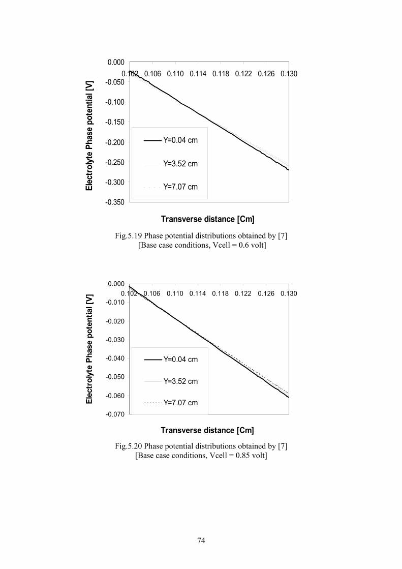
74

-0.350

-0.300

-0.250

-0.200

-0.150

-0.100

-0.050

0.0000.102 0.106 0.110 0.114 0.118 0.122 0.126 0.130

Transverse distance [Cm]

Elec

trolyt

e Ph

ase

pote

ntial

[V]

Y=0.04 cm

Y=3.52 cm

Y=7.07 cm

Fig.5.19 Phase potential distributions obtained by [7]

[Base case conditions, Vcell = 0.6 volt]

-0.070

-0.060

-0.050

-0.040

-0.030

-0.020

-0.010

0.0000.102 0.106 0.110 0.114 0.118 0.122 0.126 0.130

Transverse distance [Cm]

Elec

trol

yte

Phas

e po

tent

ial [

V]

Y=0.04 cm

Y=3.52 cm

Y=7.07 cm

Fig.5.20 Phase potential distributions obtained by [7]

[Base case conditions, Vcell = 0.85 volt]

75

5.1.7 Oxygen enrichment effects In order to alleviate mass transport losses at the cathode side, the incoming air stream

is sometimes enriched with oxygen. The effect of using pure oxygen instead of air has

been experimentally determined by [34]. Figure 5.21 shows the Polarization curves of

a fuel cell operating at two different pressures at a temperature of 50 °C for both air

and pure oxygen that were obtained by [34].

A series of runs were made at a stoichiometric ratio of 3.0 at the cathode side and 2.4

at the anode side. The anode pressure was fixed at 3.0 bar while the cathode pressure

was 5.0 bar for one simulation and 3.0 for the other and the two feed streams were

assumed fully humidified. In all, the results as shown in Fig.5.22 exhibit the same

trend as those displayed in fig.5.21 however, quantitative comparison can not be made

since the conditions of the experiment of [34] were not fully reported.

Fig.5.23 displays the 2D contours of the oxygen mass fraction throughout the cell.

It is evident that the "down-the-channel" effect decreased and thus the concentration

overpotential along the gas channel is less than the case where air is used instead of

pure oxygen leading to higher cell current densities and better cell performance.

Fig.5.21 experimentally measured fuel cell performance at 50 °C for air and pure oxygen

76

00.10.20.30.40.50.60.70.80.9

11.11.2

0 0.1 0.2 0.3 0.4 0.5 0.6 0.7 0.8 0.9 1


Cel

l Pot

entia

l [V

]

Air- 5 barPure Oxygen- 5 barAir- 3 barPure Oxygen- 3 bar

Fig.5.22 Computed polarization curves under Air

And pure oxygen operating conditions

Fig.5.23 2-D contours of Oxygen mass fraction throughout the cell

[Base case conditions, Pure Oxygen supplied , V=0.6 Volt]

77

5.1.8 Hydrogen dilution effects

To the best of the authors' knowledge, the hydrogen dilution effect has not been

thoroughly investigated experimentally except for the data found in a meeting abstract

[20] accordingly; this data can not be considered a bench-mark. It is to be noted that,

when reformate gas is used as the anode feed; the hydrogen mole fraction at the anode

inlet is significantly lower than that in the pure hydrogen condition (i.e., hydrogen

plus water vapor only) This in turn, might lead to mass-transfer limited cell

performance especially at high current densities where hydrogen is to be abundantly

supplied to the reaction sites. A series of simulations for different hydrogen inlet

fractions at the anode were carried out to illustrate this effect. In all these simulations,

the stoichiometric flow ratios of fuel and oxidant are fixed at 2.4 and 3.0 at 1 A/cm²,

respectively. The conditions of the experiment found in [20] are not known except for

the cell temperature and hydrogen stoichiometry.Fig5.24 displays the results of the

experiment found in [20].

00.10.20.30.40.50.60.70.80.9

11.11.2

0 0.5 1 1.5 2 2.5


Cell

Pote

ntia

l [V

]

Pure Hydrogen10% Hydrogen8% Hydrogen6% Hydrogen

Fig.5.24. Experimentally determined polarization curves under H2 dilution conditions,

adapted from [20]. [Cell Temperature 80 °C, H2 stoichiometry 2.4 at 1.0 A/Cm²]

78

It shows smooth decrease in the current density with hydrogen dilution and there is no

hydrogen percentage below which the cell performance is catastrophically affected

[20]. Figure 5.25 shows the computed current density under hydrogen dilution

conditions. It is evident that it decreases to a somewhat big extent –but not as much as

the experiment-for all the current densities, in qualitative agreement with the

experiment found in [20] however quantitative comparison is not possible due to the

lack of specific information about the conditions of this experiment. The reason why

the effect of hydrogen dilution is not as much as in the experiment is that the present

model assumes the anode kinetics to be very fast and accordingly, whatever small is

the quantity of hydrogen reaching the active area of the anode catalyst layer, it is

instantly consumed by the electrochemical reaction and thus hydrogen kinetics is not

the rate-limiting step for the cell performance. In all, further more detailed study of

the hydrogen dilution effect is required both experimentally and theoretically to

determine the factors affecting this phenomenon and to accurately quantify its impact

on the cell performance. The present model takes into account the anode kinetics

through Eq.3.8 representing all the cell conditions including operation under hydrogen

dilution and low current density conditions which might not be true and is to be

scrutinized through those studies. At low current densities the consumption rate of the

hydrogen available at the reaction sites may not be high leading to saturation of the

catalyst surface with hydrogen and consequent zero order kinetics in which the rate of

the electrochemical Reaction would only depend on the electrode potential,

temperature and the active area of the catalyst and thus mass transfer limitations

would not impact the cell performance. On the contrary, at high current densities the

catalyst surface is being completely depleted of hydrogen and this might lead to very

high concentration overpotentials had the supply of hydrogen been inadequate. Those

behaviors are nonetheless not shown by the experiment in [20] which again, could not

be considered as a benchmark. It is to be noted also that the present experiment

separates the fuel utilization issue from the hydrogen dilution issue through the use of

high stoichiometric flow ratios leading to high fuel utilization conditions (which are

rarely achieved in practice) On the contrary, low fuel utilization reduces the down-

the-channel effect and thus could possibly well interact with the hydrogen dilution to

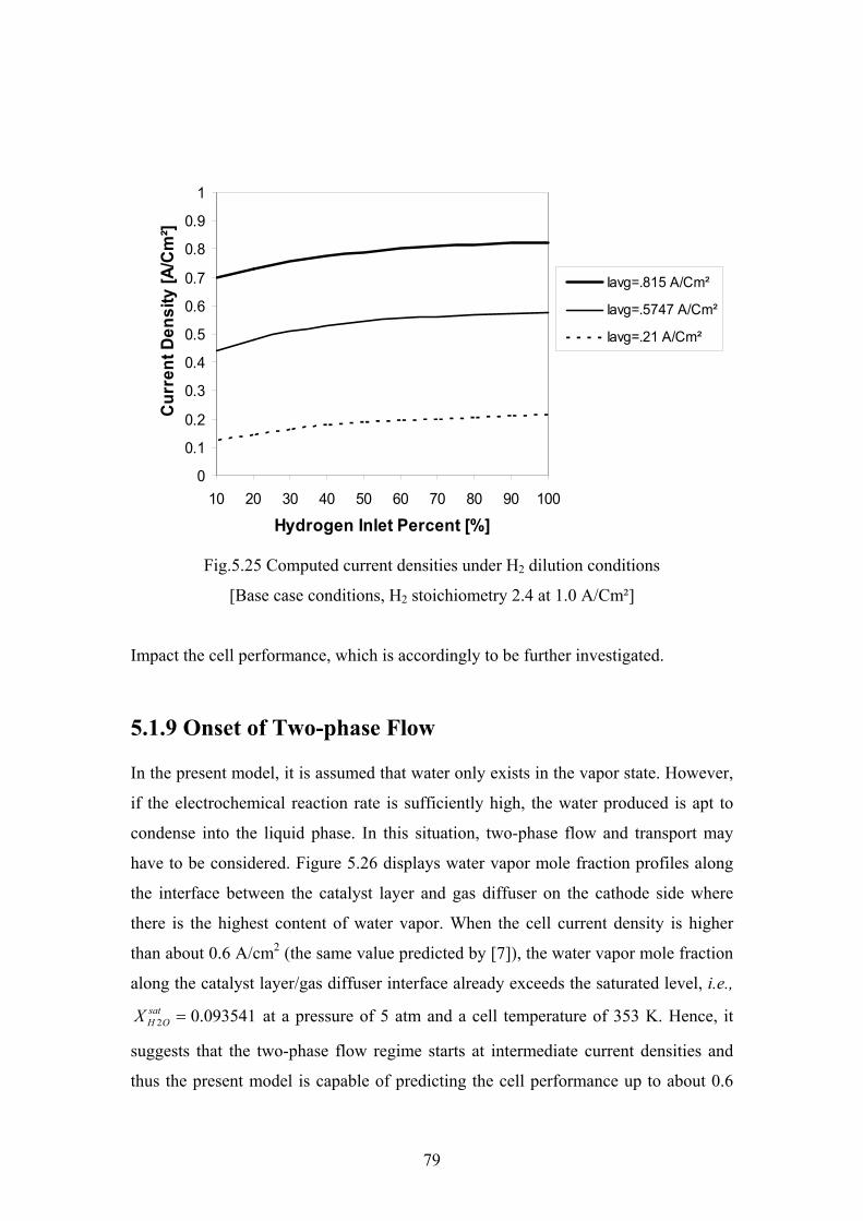
79

0

0.1

0.2

0.3

0.4

0.5

0.6

0.7

0.8

0.9

1

10 20 30 40 50 60 70 80 90 100

Hydrogen Inlet Percent [%]

Curr

ent D

ensi

ty [A

/Cm

²]

Iavg=.815 A/Cm²

Iavg=.5747 A/Cm²

Iavg=.21 A/Cm²

Fig.5.25 Computed current densities under H2 dilution conditions

[Base case conditions, H2 stoichiometry 2.4 at 1.0 A/Cm²]

Impact the cell performance, which is accordingly to be further investigated.

5.1.9 Onset of Two-phase Flow

In the present model, it is assumed that water only exists in the vapor state. However,

if the electrochemical reaction rate is sufficiently high, the water produced is apt to

condense into the liquid phase. In this situation, two-phase flow and transport may

have to be considered. Figure 5.26 displays water vapor mole fraction profiles along

the interface between the catalyst layer and gas diffuser on the cathode side where

there is the highest content of water vapor. When the cell current density is higher

than about 0.6 A/cm2 (the same value predicted by [7]), the water vapor mole fraction

along the catalyst layer/gas diffuser interface already exceeds the saturated level, i.e.,

093541.02 =satOHX at a pressure of 5 atm and a cell temperature of 353 K. Hence, it

suggests that the two-phase flow regime starts at intermediate current densities and

thus the present model is capable of predicting the cell performance up to about 0.6

80

A/cm2. Nonetheless, a single-phase analysis such as the present model and many

existing models [7, 10, 11, 13, 35, 36, and 37] still provides a good first

approximation of cell performance for current densities above 0.6 A/cm2. This is true

because the water distribution affects the electrochemical process and oxygen

transport in the air cathode primarily in two ways. First, the presence of liquid water

affects the water content in the membrane and thus slightly alters its ionic

conductivity. More important, liquid water present in the gas diffusion cathode

hampers oxygen transport to the catalyst layer [7]. However, recent two-phase

calculations[40, 41] indicated that a small amount of water is present in the cell up to

a current density of about 1.5 A/cm2and thus these effects are likely to be minimal[ 7].

0.020

0.030

0.040

0.050

0.060

0.070

0.080

0.090

0.100

0.110

0.120

0.130

0.140

0.150

0 1 2 3 4 5 6 7

Axial Distance [Cm]

Wat

er V

apor

Mol

e Fr

actio

n, X

H2O

( Iavg = 0. 711 A/Cm²)

( Iavg = 0.6075 A/Cm²)

( Iavg = 0.5022 A/Cm²)

Saturation LevelXH2O=0.09354

Onset ofTwo-phase flow regime

Fig 5.26 Computed water vapor mole fraction along the cathode GDL/CL interface

81

Fig5.27 Below displays the water vapor mole fraction profiles obtained by Um et al. It

readily shows that the onset of two-phase flow occurs at a current density of about 0.6

A/cm2 which is close to the value predicted by the present solution.

Fig5.27 Water vapor mole fraction profiles obtained by [7]


82

Chapter Six

CONCLUSIONS AND SUGGESTIONS FOR

FUTURE WORK

6.1 Introduction The present thesis work aims at developing a mathematical model that describes

the complex physical phenomena occurring inside the polymer membrane fuel cells,

to develop the CFD tool to solve the proposed model and to study the effect of the

various operating parameters on the performance of the cell. The numerical solution

obtained shed light on the interaction of the flow/transport and electrochemistry of the

PEMFC and lead to more in-depth understanding of the interrelations of the different

cell parameters. The CFD code has been validated against existing experimental work

as well as other existing numerical solutions, even though complete similarity of the

conditions of the experiments or even of the simulation parameters used in other

numerical solutions could not be attained, the results of the present numerical solution

agreed qualitatively with all of the existing experimental work and numerical

solutions. Few suggestions come to mind for building up on the existing thesis work

towards more in-depth understanding of the physics of the PEFMC and more

elaborate quantification of the performance of the cell under different operating

conditions. Those suggestions will be discussed in the next few subsections.

6.2 Conclusions of the Present Work The present model is capable of predicting the performance of the cell to high

accuracy under the different operating conditions. A thorough examination of the

results of chapter 5 leads to the following conclusions:

• Increasing the operating temperature leads to improved cell performance

because of the reduced cell internal resistance, reduced activation

overpotential, and overall improvement in the mass transport to the reaction

sites. However the maximum possible operating temperature is limited by the

maximum temperature that the membrane material can withstand without

83

being damaged and dehydration of the membrane which leads to its loss of the

protonic conductivity and thus increased cell resistance and consequent poor

cell performance.

• Increasing the cell pressure improves the cell performance up to a certain limit

beyond which any further pressurizing can not be justified.

• Controlled humidification of the feed streams is desirable to alleviate the

problem of membrane dehydration and consequent loss of protonic

conductivity but it must be rigorously assessed so as to avoid flooding of the

electrodes in which the pores are plugged with water which drastically

hampers the transport of further reactants to the reaction sites and accordingly

leads to drastic drop in the cell performance.

• Use of pure oxygen enhances the cell performance by reducing the

concentration overpotential resulting from the limited transport of oxygen to

the active reaction sites at the cathode catalyst layer.

• In a like manner, increasing the percentage of hydrogen in the reformate

alleviates mass transport limitations on the anode side and thus leading to

improved cell performance.

• The model is capable of predicting the cell performance within a relatively

broad span of the cell operating voltages beyond which the two-phase flow

regime starts and more elaborate mathematical model is then required to

describe the cell physical phenomena.

6.3 Recommendations for Future Work,

The aim of the following recommendations is to improve the model presented in this

thesis work so as to gain a more thorough understanding of the physics underlying the

operation of the polymer membrane fuel cells.

• Modifying the model to take into account transient effects, in this thesis work

we solved a steady-state model and thus our model is not capable of prediction

of the fuel cell response to varying load conditions.

• Modifying the model to take into account the two-phase flow phenomenon

occurring inside the cell.

84

• More elaborate determination of the different simulation parameters including

electrochemistry parameters like the cathodic exchange current density and its

variation with the cell operating conditions and the diffusivity of the different

mixture components especially that of the water vapor throughout the

membrane (In this thesis work the effect of membrane water content has been

ignored and Also the membrane protonic conductivity was assumed to vary

only with the temperature whereas it is known to vary with the membrane

water content as well ).

• More accurate determination of the open circuit voltage. Due to losses

resulting from undesired species crossover from one electrode through the

electrolyte and internal currents, the actual open circuit voltage is below the

theoretical value (use has been made of the Nernst equation in this thesis work

for the majority of the simulations).besides, the experiment had shown that it

increases with the temperature on the contrary to the predictions of Nernst

equation however the experimental correlation (that was employed for the

effect-of-temperature simulation) does not reflect the effect of the change of

the operating pressures on the open circuit voltage.

• Studying the different types of flow field design (serpentine, parallel flow,

interdigitated …etc) and its effect on the cell performance regarding pressure

drop and uniformity of reactants at the gas channel/porous media interface.

Such a simulation would involve more detailed three-dimensional model of

the fuel cell.

• Conducting a water management study which will ultimately lead to

determination of the required humidification levels for the different feed

streams and avoidance of the conditions leading to membrane dehydration.

• Conducting a heat management study to determine the heat generated within

the fuel cell resulting from ohmic heating, phase change…etc and the heat

dissipation to the coolant, cell body...etc so that we can avoid the conditions

leading to high cell temperatures which might lead to damage of the polymeric

membrane. Such a study would involve modifying the model by solving the

energy equation (in this thesis work the temperature was assumed constant.)

and incorporating the different sources of heat generation and dissipation into

the energy equation and then to solve for the temperature.

85

• More elaborate study of the anode stream dilution effect including of course

the CO poisoning effect. Such a study would require an in-depth

understanding of the anode kinetics where CO is present in the anode stream,

and might lead to enhancement of the cell tolerance levels to CO.

86

REFERENCES

1. US-DOE, Office of Fossil Energy, FETC, “Fuel Cell Handbook”,

Morgantown, WV, 2000.

2. von Spakovsky M.R., Nelson D.J, and Ellis M.W. ME 5984, "Fuel Cell

Systems", Class Notes, Virginia Polytechnic and State University, Blacksburg,

VA, Spring 2000.

3. Hamann, C., Hamnett, A., and Vielstich, W., "Electrochemistry", Wiley-VCH,

New York, New York, 1998.

4. Yammoto, O., Solid Oxide Fuel Cells, "Fundamental Aspects and Prospects",

Eletcrochemica Acta, Vol.45, 2000, pp. 2423-2435.

5. Mench, M.M., Wang, C.Y., and Thynell, S.T., "An Introduction to Fuel Cells

and Related Transport Phenomena", Accepted for publication in Journal of

Transport Phenomena, 2001.

6. Bard, A.J., and Faulkner, L.R., "Electrochemical Methods", John Wiley and

Sons, New York, New York, 1980, pp.101.

7. Um, S., Wang, C.Y., and Chen, K.S.,"Computational Fluid Dynamics

Modeling Of Proton Exchange Membrane Fuel Cells",J Electrochem.Soc.,

Vol.147, No.12, 2000, pp. 4485

8. Sherif, S.A., Barbir, F., and Veziroglu, T.N., "Hydrogen Energy System:

Fundamentals and Applications." Asia Pacific Tech Monitor,

January/February 1999.

9. Olsommer B., "Mathematical Model for a PEM Fuel Cell", Internal

Document, Energy Management Institute, Mechanical Engineering, Virginia

Polytechnic and State University, Blacksburg, VA, 2000.

10. Springer, T.E., Zawodzinski, T.A., and Gottesfeld , S., "Polymer Electrolyte

Fuel Cell Model", Journal of the Electrochemical Society, Vol. 138, No. 8,

1991, pp. 2334-2342,(a).

11. Bernardi, D.M.,and Verbrugge, M.W., , "A Mathematical Model of the Solid-

Polymer-Electrolyte Fuel Cell", Journal of the Electrochemical Society, Vol.

139, No. 9,1992, pp. 2477-2491.

87

12. Weisbrod, K.R., Vanderborgh, N.E., and Grot S.A., "Modeling of Gaseous

Flows within Proton Exchange Membrane Fuel Cells" , Proceedings 1996 Fuel

Cell Seminar, Orlando, FL, 1996, pp. 635-638.

13. Gurau, V., Kakac, S., and Liu, H., "Mathematical Model for Proton Exchange

Membrane Fuel Cells", AES Vol. 38, Proc. of the ASME Advanced Energy

Systems Division, 1998, pp. 205-214,ASME.

14. Eikerling, M., Kharkats, YuI., Kornyshev, A.A., and Volfkovich, YuM.,

"Phenomenological theory of electro-osmotic effect and water management in

polymer electrolyte proton-conducting membranes", Journal of the

Electrochemical Society, Vol. 145 No. 8, 1998, pp. 2684-2699.

15. Yi, J.S., Nguyen, T.V., "Multicomponent Transport in Porous Electrodes of

Proton Exchange Membrane Fuel Cells Using Interdigitated Gas Distributors",

Journal of the Electrochemical Society, Vol. 146, No. 1, 1999, pp. 38-45.

16. Eaton, B.M.,"One Dimensional, Transient Model of Heat, Mass, and Charge

Transfer in a Proton Exchange Membrane", MSC Thesis, Mechanical

Engineering, Virginia Polytechnic and State University, Blacksburg, 2001,

VA.

17. Genevey, D.B.,"Transient Model of Heat, Mass, and Charge Transfer as well

as Electrochemistry in the Cathode Catalyst Layer of a PEMFC", MSC Thesis,

Mechanical Engineering, Virginia Polytechnic and State University,

Blacksburg, 2001, VA.

18. Pasaogullari, U., Wang, C.Y., "Computational Fluid Dynamics Modeling of

Proton Exchange Membrane Fuel Cells Using Fluent®", Fluent User Group

Meeting, Manchester, 2002, NH.

19. Berning, T., Djilali, N.,"Three-dimensional computational analysis of

transport phenomena in a PEM fuel cell—a parametric study", Journal of

Power sources, Vol.124, 2003, pp. 440–452.

20. Rockward, T., Zawodzinski, T., Bauman, J., Uribe, F., Valerio, J., Springer,

T., and Gotteesfeld, S., " The performance of polymer electrolyte membrane

fuel cells operating on diluted hydrogen", The Electrochemical Society

Meeting Abstracts, Vol. 99-1, Seattle, May 2-6, 1999, WA.

88

21. Hong, J.K.,Zook, L.A., Inbody, M.,Tafoya, J., and Vanderborgh, N.E.,

Abstract 570, The Electrochemical Society Meeting Abstracts, Vol. 99-1,

Seattle, May 2-6, 1999,WA.

22. Meng, H., Wang, C.Y.,"Electron Transport in PEFCs" , Journal of the

Electrochemical Society, Vol. 151 (3), 2004, A358-A367.

23. Berning, T.,"Three-Dimensional Computational Analysis of Transport

Phenomena in a PEM Fuel Cell", Ph.D. Thesis, Department of Mechanical

Engineering, University of Victoria, 2002.

24. Parthasarathy, A., Srinivasan, S., and Appleby, J., J. Electrochem Soc.,

Vol.139, 1992, pp.2530.

25. Bird, R.B., Stewart, W.E., and Lightfoot, E.N., "Transport Phenomena", John

Wiley & Sons, New York, 1960.

26. Kumar, A. , and Reddy, R,G.,"Modeling of Polymer Electrolyte Membrane

Fuel Cell with Metal Foam in the Flow Field of the Bipolar/End

Plate",J.Power Sources, 114,2003,pp.56,62.

27. Ticianelli, E.A., Derouin, C.R., and Srinivasan, S., J. Electroanal. Chem.,

1988, pp.251, 275.

28. Bernardi, D.M., and Verbrugge, M.W., AIChE J., 37, 1991, pp.1151.

29. Fluent Inc, "Fluent 6.0 User's Manual ", Centerra Resource Park, Lebanon,

2000, NH.

30. Versteeg, H.K., and Malalasekera, W., "An Introduction to Computational

Fluid Dynamics", Addison Wesley Longman, London (1995).

31. Huang, P.G., and Leschziner, M.A., "An Introduction and Guide to the

Code"TEAM", University of Manchester, 1984.

32. Gustavo, G., and Jen, T.C., "Numerical Analysis of the Hydrodynamics of the

Flow in an Axially Rotating Heat Pipe", Internal report, Department of

Mechanical Engineering, University of Wisconsin, Milwaukee, Milwaukee,

2001, WT53211.

33. Patankar, S.V.,"Numerical Heat Transfer and Fluid Flow", Hemisphere

Publishing Corporation, USA, 1980.

34. Kim, J., Lee, S.M., Srinivasan, S., and Chamberlin, C.E., "Modeling of proton

exchange membrane fuel cell performance with an empirical equation", J.

Electrochem. Soc. 142 (8) ,1995, pp. 2670–267.

89

35. Beavers, G.S., Sparrow, E.M., and Mangnuson, R.A.,"Experiments on

Coupled Parallel Flows in a Channel and a Bounding Porous Medium", Trans.

ASME, J. Basic Eng.,Vol. 30, 1970, pp.843.

36. Dagan, G., "Flow and Transport in Porous Formations", Springer-Verlag,

Berlin , 1989.

37. Springer, T.E., Wilson, M.S., and Gottesfeld, S., Journal of the

Electrochemical Society, Vol. 140, 1993, pp. 3513.

38. Fuller, T.F., and Newman, J., J. Electrochem.soc., Vol.140, 1993, pp.1218.

39. Nguyen, T.V., and White, R.E., J. Electrochem.soc., Vol.140, 1993, pp.2178

40. Wang, C.Y., Wang, Z.H., and Pan, Y., Proceedings of ASME Heat Transfer

Division, HTD-Vol, 364-1, ASME, New York, 1999, P.351.

41. Nguyen, T.V.,"Tutorials in Electrochemical-Engineering Mathematical

Modeling", R. F. Savinell, J. M. Fenton, A. West, S. L. Scanlon, J.

Weidner, Editors, PV 99-14, p. 222, The Electrochemical Society

Proceedings Series , Pennington, NJ, 1999.

90

APPENDICES

APPENDIX A

Flow Chart of the Original TEAM Code

MODED

TEAM

CALL SET

CALL GRID

CALL INLET

CALL OUTPI

CALL PROPS

CALL CALCU

CALL CALCV

CALL CALCP

CALL CALCTE

CALL CALCED

CHECKCONVERGENCE

CRITERIA

CALL OUTP

STOP

USER

SET

GRID

INLET

OUTPI

PROPS

MODU

MODV

MODP

MODTE

OUTP

CALCTE

CALCED

CALCP

CALCV

CALCU

91

APPENDIX B

Flow Chart of the VTC Numerical Algorithm

Start

- Input cell potential,temperature,pressure ,relativehumidity,hydrogen inlet %, Oxygen inlet %

- Solve Momentum equations , species transportequations for mass fractions of water vapor, oxygen,hydrogen and membrane phase potential equation

-Calculate the cell's local and avergare currentdensities

- Check for convergence of momentum, massfractions, potential fields, current density

If converged

STOP

- Update mixture density,viscosityand source terms

If not converged

-Initialize axial,transverse velocities,species massfractions and membrane phase potential

92

APPENDIX C

Flow Chart of the PEMCU Code

MODYO2

PEMCU

CALL SET

CALL GRID

CALL INLET

CALL OUTPI

CALL PROPS

CALL CALCU

CALL CALCV

CALL CALCP

CALL CALCYH2O

CALL CALCYO2

CHECKCONVERGENCE

CRITERIA

CALL OUTP

STOP

USER

SET

GRID

INLET

OUTPI

PROPS

MODU

MODV

MODP

MODYH2O

OUTP

CALCYH2O

CALCYO2

CALCP

CALCV

CALL CALCYH2

CALL CALCPH

CALCYH2

CALCPH

MODYH2

MODPH

CALCU

93

APPENDIX D

Base Case Parameters

• Most of theses parameters are taken from [7] and [11]

Physical Quantity Value*

Cathode pressure 5 bar Anode pressure 3 bar

Air stoichiometric flow ratio ζ+ 3. Fuel stoichiometric flow ratio ζ+ 2.8

Cell temperature 80 °C Relative humidity of inlet air 0.0 % Relative humidity of inlet fuel 100%

Reference exchange current density × area of anode, refaaJ 1.4E11 A/m3

Reference exchange current density × area of cathode, refcaJ 6000. A/m3

Oxygen diffusivity in gas 5.2197E-06 m2/s Hydrogen diffusivity in gas 2.63E-06 m2/s

Water vapor diffusivity at the anode side 0.733E-6 m2/s Water vapor diffusivity at the cathode side 0.49E-06 m2/s

Dissolved oxygen diffusivity in active layer and membrane 2.0E-8 m2/s Dissolved hydrogen diffusivity in active layer and membrane 2.59E-10 m2/s

Hydraulic permeability of membrane, kp 1.8E-18 m2

Permeability of backing layer, K 1.76E-11 m2 Electrokinetic permeability, kФ 7.18E-20 m2

Fixed site charge, Zf -1 Anodic transfer coefficient,αa 2

Cathodic transfer coefficient,αa 2 H2 Concentration dependence exponent γH2 0.5 O2 Concentration dependence exponent γO2 1.

Backing layer porosity, ε 0.4 Membrane porosity, εm 0.28

Membrane Volume fraction in the Catalyst layer , εmc 0.5 Fixed charge concentration, Cf 1.2 E-3 mol/cm3

Reference hydrogen concentration CH2,ref 40. mol/cm3 Reference oxygen concentration CO2,ref 40. mol/cm3

Gas channel length, L 7.112 cm Gas channel width 0.0762 cm

Backing layer width 0.0254 cm Catalyst layer width 0.00287 cm

Membrane width 0.023 cm

xv

ملخص البحث

ال ي مج دة ف ادر الواع ن المص ود م ا الوق ر خالي ةتعتب اج الطاق ن إنت ه م ز ب ا تتمي را لم نظ

ن ة ع وتية الناجم ة والص ات الحراري اض االنبعاث ع انخف ة م اءة الحراري ي الكف اع ف ارتف

ين ة ب اعالت الداخلي واءالتف ود واله درات . الوق ا بق ن توفيره غيل ويمك هولة التش ز بس ا تتمي ا أنه آم

ف م مختل ة تالئ ات المتنوع ييرتطبيق يارات وتس اء ت الس د الكهرب تخدام .ولي غيلها باس ن تش ا يمك آم

. أنواع مختلفة من الوقود مما يساهم في سهولة انتشارها آتقنية جديدة في مختلف مواقع اإلنتاج

ذا الب الل ه اد خ ائى األبع ى ثن وذج رياض وير نم م تط ث ت اد، ح ورىأح تق، الط رمس

وليمرى اء الب ود ذات الغش ا الوق اة أداء خالي Polymer Electrolyte Membraneلمحاآ

Fuel Cell.ائى ل الكهروآيمي دل التفاع ة مع اره دراس ى اعتب وذج ف ذا النم ذ ه ث يأخ اديناميك، حي

.الموائع واالنتقال متعدد المرآبات

د الل وق ق خ الحة للتطبي ظ ص ادالت الحف ن مع دة م ة واح تخدام مجموع م اس ر ت ال غي المج

ا وات الغ ن قن ون م انس والمك اريةةالطبق، اتزالمتج ة ، Gas Diffusion Layer اإلنتش طبق

وليمرى اء الب ز والغش امج . المحف تخدام برن ا باس ا PEMCU وحله ويره خصيص م تط ذى ت وال

ى وذج الرياض ذا النم ل ه اءالح امج بن ى برن ام TEAM عل ويره ع م تط ذى ت ة ١٩٨٤ ال بجامع

.مانشستر اإلنجليزية لدراسة نفاث اضطرابى مرتطم

اء ين الكيمي دة ب ة والمعق أثيرات المتداخل ى الت وء عل اء الض ددى بإلق ل الع ام الح د ق ذا وق ه

ة ةاميكانيك، الكهربي ل الخلي ات داخ دد المرآب ال متع ع واالنتق تخدام . الموائ م اس د ت امج وق البرن

غط ل الض ا مث ن الخالي وع م ذا الن ى أداء ه ة عل غيل المختلف ل التش أثير عوام ة ت ى دراس ددى ف ، الع

رارة ة الح يط،درج ى الخل دروجين ف بة الهي خ...نس ة . ال اتج بالتجرب ددى الن ل الع ة الح ت مقارن وتم

ول العدد ة والحل ةالعملي ت المقارن ة وأثبت ة المتاح نهمي د بي اق جي ود اتف . وج

xvi

نمذجة رياضية ومحاآاة عددية لخاليا الوقود ذات الغشاء البوليمرى

إعداد

محمدعبد الغنىعمار محمد / مهندس

عبد الغنىدسمير محم/ األستاذ الدآتور عضو

ل أبو اللي محمد مرسى محسن/األستاذ الدآتور عضو

هاني أحمـد صفـي الدين خاطـر/ ستاذ الدآتوراأل رئيسىمشرف

هنـداوي سالـم محمــد/ األستاذ الدآتور مشرف

آليــة الهندســة ، جامعــة القاهــرة الجيـزة ، جمهوريـة مصـر العربيــة

٢٠٠٤

رسالة مقدمة إلى آلية الهندسة، جامعة القاهرةآجزء من متطلبات الحصول على درجة الماجستير

في هندسة القوى الميكانيكية

يعتمد من لجنة الممتحنين

xvii


إعداد

محمدعبد الغنىعمار محمد / مهندس

تحت إشـــراف


٢٠٠٤

هاني أحمـد صفـي الدين خاطـر/ األستاذ الدآتور

قسـم هندســة الـقوى الميكانيكـية

آليـة الهندســة، جامعــة القاهــرة

لى آلية الهندسة، جامعة القاهرةرسالة مقدمة إآجزء من متطلبات الحصول على درجة الماجستير


هنـداوي سالـم محمــد/ األستاذ الدآتور


آليـة الهندســة، جامعــة القاهــرة

عمـرو محمـد علي عبـد الرءوف/ الدآتور


، جامعــة القاهــرةآليـة الهندســة

xviii


إعداد

محمدعبد الغنى محمدعمار/ مهندس


٢٠٠٤

رسالة مقدمة إلى آلية الهندسة، جامعة القاهرةآجزء من متطلبات الحصول على درجة الماجستير


MATHEMATICAL MODELING AND NUMERICAL SIMULATION OF POLYMER ELECTROLYTE MEMBRANE FUEL...

Documents

Transcript of MATHEMATICAL MODELING AND NUMERICAL SIMULATION OF POLYMER ELECTROLYTE MEMBRANE FUEL...