Math 636 - Mathematical Modeling - Modeling Diabetes

IntroductionModeling GTT

Diabetes in NOD Mice

Math 636 - Mathematical Modeling

Modeling Diabetes

Joseph M. Mahaffy,〈[email protected]〉

Department of Mathematics and StatisticsDynamical Systems Group

Computational Sciences Research Center

San Diego State UniversitySan Diego, CA 92182-7720

http://jmahaffy.sdsu.edu

Fall 2017

Joseph M. Mahaffy, 〈[email protected]〉 Modeling Diabetes — (1/50)



Outline

1 IntroductionGlucose MetabolismType 1 or Juvenile Diabetes

2 Modeling GTTLinearized GTT ModelExample

3 Diabetes in NOD MiceModeling Diabetes in NOD MiceQuasi-Steady State ModelParameters and Bifurcation




Glucose MetabolismType 1 or Juvenile Diabetes

Introduction

Introduction

Diabetes is a disease, characterized by excessive glucose in theblood stream.

Currently, there is an epidemic of diabetes.

Modern unhealthy lifestyles are dramatically different fromhow humans survived when they evolved from smallnomadic hunter-gatherer societies.Then food was difficult to find.

There are two forms of diabetes.

Type 1, often called juvenile diabetes.Type 2, often referred to as adult onset diabetes (whichnow occurs in children as young as 5).

Our studies concentrate on Type 1 diabetes, which is anautoimmune disease and represents only 10% of all cases ofdiabetes.





Glucose Metabolism

Glucose Metabolism

Ingest food, which breaks down to simple sugars.Blood absorbs sugar, which raises blood glucose concentration.β cells in pancreas respond and insulin is released.

Cells increase glucose uptake.

Insulin facilitates glucose transport across cell membranes, especially

in skeletal muscles.

Glucose converted to glycogen, the preferred energy storage of cells.

Blood sugar level decreases.Body tightly regulates glucose levels.


http://jmahaffy.sdsu.edu




Type 1 or Juvenile Diabetes - Overview

Type 1 or Juvenile Diabetes - Overview

Diabetes mellitus results from the loss of β cells, anauto-immune disease.

Hereditary disease - about 4-20 per 100,000 people.Peak diagnosis occurs around age 14.

Insulin production is severely reduced.

10% of diabetes cases are Type 1, while 90% are Type 2 (wherecells become insulin resistant, mostly in obese individuals).

Treatment is regular injections of insulin - transplants areusually attacked by immune system.

Modern modeling methods and implanted devices allowcontinuous monitoring of the body glucose levels and computercontrolled release of insulin (still experimental).





Type 1 or Juvenile Diabetes - Symptoms and Diseases

Type 1 or Juvenile Diabetes - Symptoms and Diseases

Classic Symptoms

Polyphagia (hungry)Polydipsia (thirsty)Polyuria (frequent urination)Other symptoms

Blurred vision, fatigue, weight loss, poor wound healing

Diseases

Increased heart disease - Atherosclerosis from low insulinBlindness (retinopathy) - Increased pressure in eyeNerve damage (neuropathy)Kidney damage (nephropathy)

Current prognosis is premature death.




Linearized GTT ModelExample

Modeling Glucose Metabolism

Modeling Glucose Metabolism: The regulation of glucose in theblood begins with the ingestion of food.

Hormones: β-cells in the pancreas to release insulin into the blood(along with a number of other hormones), where insulin facilitates ofglucose transport across cell membranes and conversion of glucose toglycogen in the liver.

Other hormones include:

Epinephrine (adrenalin) is released to break down theglycogen.Glucocorticoids help metabolize carbohydrates.Growth hormone can block the effects of insulin.

Many other hormones regulate glucose levels in the blood,creating a complex regulatory system.





Diabetes Detection

Diabetes Detection: There are 3 common tests.

Type 1 diabetes runs in families, so family members are tested.

FPG (Fasting Plasma Glucose) examines blood after an 8-hour fast - over126 mg/dL is diabetic, while under 100 mg/dL is normal.

A1C (Glycated Hemoglobin) examines blood after an 8-hour fast - over6.5% is diabetic, while under 5.7% mg/dL is normal.

OGTT (Oral Glucose Tolerance Test) fast for 8 hr, then given largeamount of glucose and tested over 2 hrs - over 200 mg/dL on any test isdiabetic, while under 140 mg/dL is normal.

Glucose Tolerance Test is a more accurate follow-up test for diabetes.

Subject fasts for 12 hours.

Subject rapidly ingests a large amount of glucose (100 g of glucose, which isabout 2.5× a can of Coke).

The blood sugar is monitored for 3-6 hrs, and these data are fit to theAckerman model (below).





Modeling GTT 1

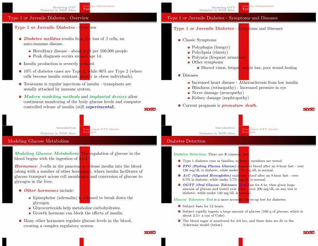
Modeling GTT: Glucose in the blood, G(t), begins with the rapidingestion of glucose, J(t).

This stimulates the release of insulin, I(t), and other hormones toregulate G(t).

This can be written as the model:

dG

dt= f1(G, I) + J(t),

dI

dt= f2(G, I).

G I

J(t)





Modeling GTT 2

Modeling GTT: Glucose regulation is complex, but we develop asimple model that can be fit with a few parameters.

More complex models have been developed to match different types offood intake for tighter regulation of people with diabetes.

Modeling Assumptions:

Assume the fasting for 8-12 hours takes the body into ahomeostasis.

The body is in a quasi-equilibrium with glucose at a level G0

and insulin at a level I0.

Assume the rapid ingestion of glucose makes J(t) like aδ-function only affecting the initial conditions.

The quasi-equilibrium assumption allows a perturbationanalysis using

g(t) = G(t)−G0 and i(t) = I(t)− I0.





Linearized GTT Model 1

For the model,

dG

dt= f1(G, I) + J(t),

dI

dt= f2(G, I),

the quasi-equilibrium assumption gives:

f1(G0, I0) = f2(G0, I0) = 0.

Expanding the general model to linear terms with these definitions gives thelinearized perturbation mode:

dg

dt=

∂f1(G0, I0)

∂gg +

∂f1(G0, I0)

∂ii,

di

dt=

∂f2(G0, I0)

∂gg +

∂f2(G0, I0)

∂ii,

where g(t) and i(t) are the linearized perturbed variables.






Next we examine the partial derivatives of the functions, f1 and f2, with ourunderstanding of the physiology of glucose and insulin.

Physiologically, an increase in glucose in the blood stimulates tissue uptake ofglucose and glycogen storage in the liver:

∂f1(G0, I0)

∂g= −m1 < 0.

An increase in insulin facilitates the uptake of glucose in tissues and the liver:

∂f1(G0, I0)

∂i= −m2 < 0.

However, increases in blood glucose result in the release of insulin:

∂f2(G0, I0)

∂g= m4 > 0.

Increases in insulin result increased metabolism of excess insulin:

∂f2(G0, I0)

∂i= −m3 < 0.






With these definitions, the linearized system is written:

(

gi

)

=

(

−m1 −m2

m4 −m3

)(

gi

)

,

where g = dg/dt and similarly for i(t).

The characteristic equation for this linear system is given by

det

∣

∣

∣

∣

−m1 − λ −m2

m4 −m3 − λ

∣

∣

∣

∣

= λ2 + (m1 +m3)λ +m1m3 +m2m4 = 0.

Since the mi > 0, all coefficients of the characteristic equation are positive.

From ODEs (think damped spring mass system), this implies that all theeigenvalues, λ, are either complex with negative real parts or both eigenvaluesare negative.

A stable node is expected of a self-regulatory system.






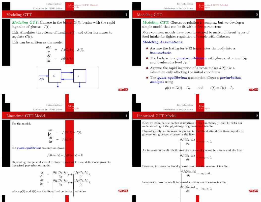
The characteristic equation is:

λ2 + (m1 +m3)λ+m1m3 +m2m4 = 0.

Only the blood glucose level in the GTT is measured, so only need the linearizedsolution for g(t).

We expect the underdamped situation with complex eigenvalues.

Physiologically, think of the body’s response to a “sugar high” (maximum of bloodglucose), which is followed after an hour or two by a “sugar low” (minimum ofblood glucose below equilibrium) that encourages more eating.

Thus, the general solution satisfies:

g(t) = e−αt(c1 cos(ωt) + c2 sin(ωt)),

where

α =m1 +m3

2and ω =

1

2

√

4(m1m3 +m2m4)− (m1 +m3)2.






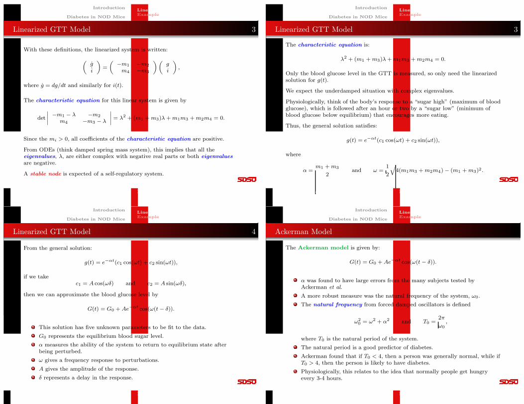
From the general solution:

g(t) = e−αt(c1 cos(ωt) + c2 sin(ωt)),

if we takec1 = A cos(ωδ) and c2 = A sin(ωδ),

then we can approximate the blood glucose level by

G(t) = G0 + Ae−αt cos(ω(t − δ)).

This solution has five unknown parameters to be fit to the data.

G0 represents the equilibrium blood sugar level.

α measures the ability of the system to return to equilibrium state afterbeing perturbed.

ω gives a frequency response to perturbations.

A gives the amplitude of the response.

δ represents a delay in the response.





Ackerman Model

The Ackerman model is given by:

G(t) = G0 + Ae−αt cos(ω(t − δ)).

α was found to have large errors from the many subjects tested byAckerman et al.

A more robust measure was the natural frequency of the system, ω0.

The natural frequency from forced damped oscillators is defined

ω20 = ω2 + α2 and T0 =

2π

ω0,

where T0 is the natural period of the system.

The natural period is a good predictor of diabetes.

Ackerman found that if T0 < 4, then a person was generally normal, while ifT0 > 4, then the person is likely to have diabetes.

Physiologically, this relates to the idea that normally people get hungryevery 3-4 hours.





Example 1

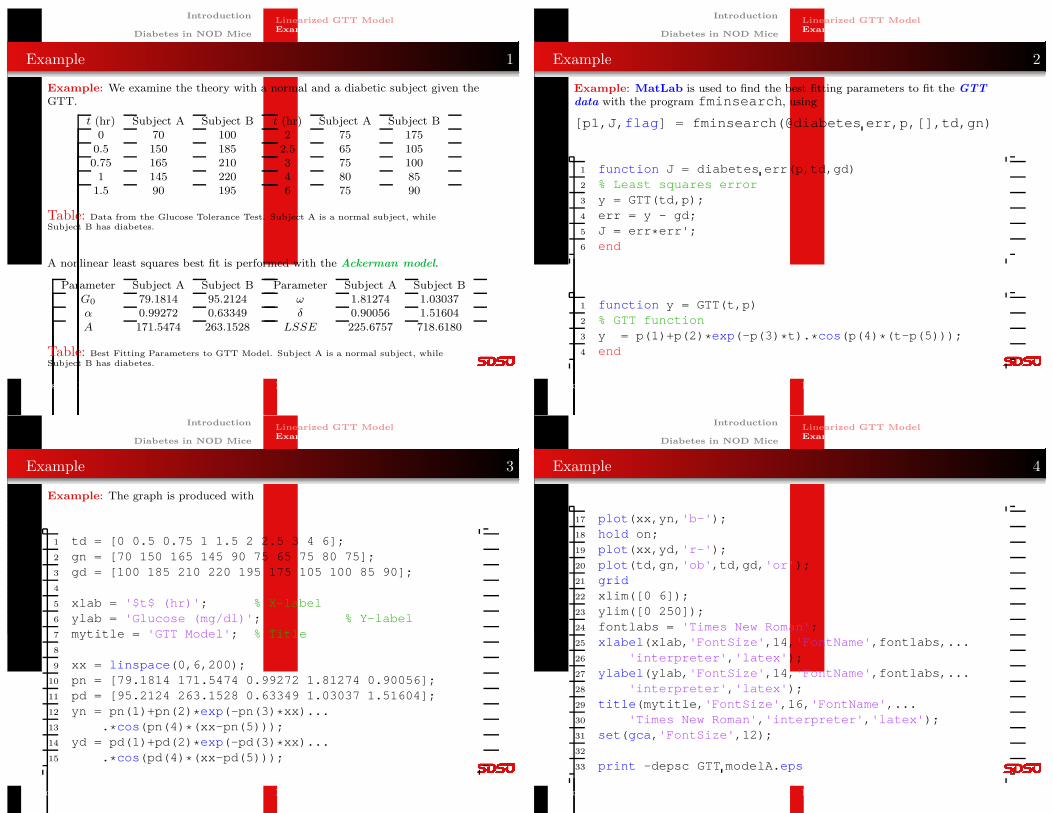
Example: We examine the theory with a normal and a diabetic subject given theGTT.

t (hr) Subject A Subject B t (hr) Subject A Subject B0 70 100 2 75 1750.5 150 185 2.5 65 1050.75 165 210 3 75 1001 145 220 4 80 851.5 90 195 6 75 90

Table: Data from the Glucose Tolerance Test. Subject A is a normal subject, whileSubject B has diabetes.

A nonlinear least squares best fit is performed with the Ackerman model.

Parameter Subject A Subject B Parameter Subject A Subject BG0 79.1814 95.2124 ω 1.81274 1.03037α 0.99272 0.63349 δ 0.90056 1.51604A 171.5474 263.1528 LSSE 225.6757 718.6180

Table: Best Fitting Parameters to GTT Model. Subject A is a normal subject, whileSubject B has diabetes.





Example 2

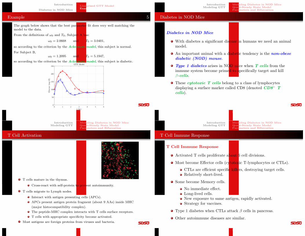
Example: MatLab is used to find the best fitting parameters to fit the GTTdata with the program fminsearch , using

[p1,J, flag ] = fminsearch(@diabetes err,p,[],td,gn)

1 function J = diabetes err(p,td,gd)2 % Least squares error3 y = GTT(td,p);4 err = y - gd;5 J = err * err';6 end

1 function y = GTT(t,p)2 % GTT function3 y = p(1)+p(2) * exp (-p(3) * t). * cos (p(4) * (t-p(5)));4 end





Example 3

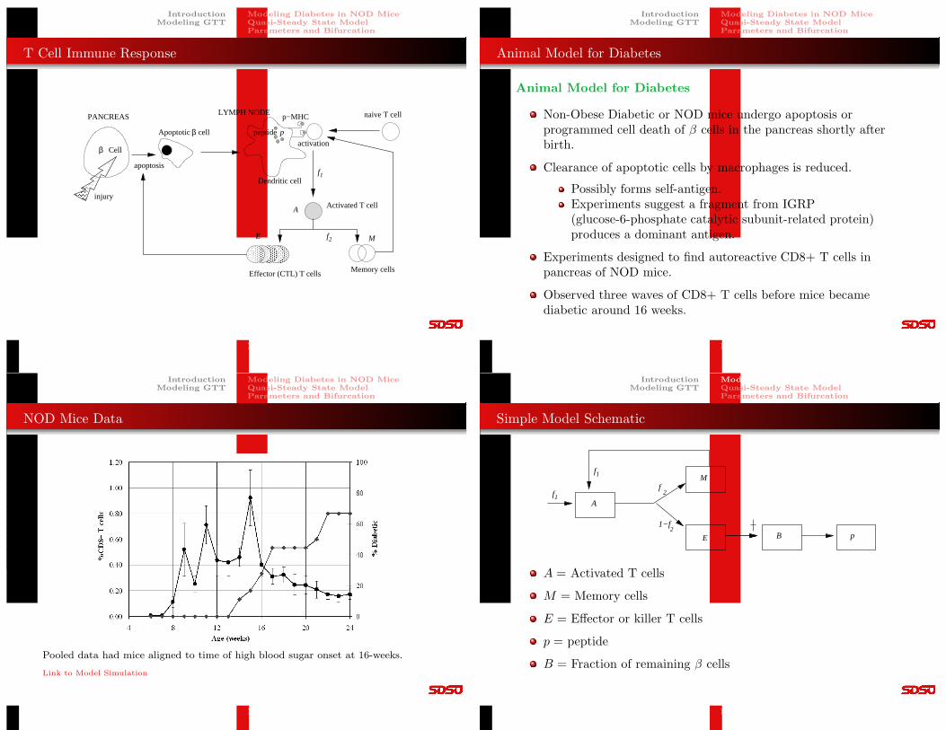
Example: The graph is produced with

1 td = [0 0.5 0.75 1 1.5 2 2.5 3 4 6];2 gn = [70 150 165 145 90 75 65 75 80 75];3 gd = [100 185 210 220 195 175 105 100 85 90];4

5 xlab = '$t$ (hr)' ; % X-label6 ylab = 'Glucose (mg/dl)' ; % Y-label7 mytitle = 'GTT Model' ; % Title8

9 xx = linspace (0,6,200);10 pn = [79.1814 171.5474 0.99272 1.81274 0.90056];11 pd = [95.2124 263.1528 0.63349 1.03037 1.51604];12 yn = pn(1)+pn(2) * exp (-pn(3) * xx)...13 . * cos (pn(4) * (xx-pn(5)));14 yd = pd(1)+pd(2) * exp (-pd(3) * xx)...15 . * cos (pd(4) * (xx-pd(5)));





Example 4

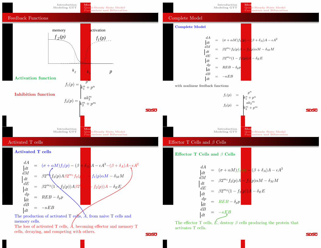
17 plot (xx,yn, 'b-' );18 hold on;19 plot (xx,yd, 'r-' );20 plot (td,gn, 'ob' ,td,gd, 'or' );21 grid22 xlim([0 6]);23 ylim([0 250]);24 fontlabs = 'Times New Roman' ;25 xlabel (xlab, 'FontSize' ,14, 'FontName' ,fontlabs,...26 'interpreter' , 'latex' );27 ylabel (ylab, 'FontSize' ,14, 'FontName' ,fontlabs,...28 'interpreter' , 'latex' );29 title (mytitle, 'FontSize' ,16, 'FontName' ,...30 'Times New Roman' , 'interpreter' , 'latex' );31 set ( gca , 'FontSize' ,12);32

33 print -depsc GTT modelA. eps





Example 5

The graph below shows that the best parameter fit does very well matching themodel to the data.

From the definitions of ω0 and T0, Subject A has:

ω0 = 2.0668 and T0 = 3.0401,

so according to the criterion by the Ackerman model, this subject is normal.

For Subject B,ω0 = 1.2095 and T0 = 5.1947,

so according to the criterion by the Ackerman model, this subject is diabetic.

0 1 2 3 4 5 60

50

100

150

200

250




Modeling Diabetes in NOD MiceQuasi-Steady State ModelParameters and Bifurcation



With diabetes a significant disease in humans we need an animalmodel.

An important animal with a diabetic tendency is the non-obesediabetic (NOD) mouse.

Type 1 diabetes arises in NOD mice when T cells from theimmune system become primed to specifically target and killβ-cells.

These cytotoxic T cells belong to a class of lymphocytesdisplaying a surface marker called CD8 (denoted CD8+ Tcells).





T Cell Activation

T cells mature in the thymus.

Cross-react with self-protein to prevent autoimmunity.

T cells migrate to Lymph nodes.

Interact with antigen presenting cells (APCs).

APCs present antigen protein fragment (about 9 AAs) inside MHC

(major histocompatibility complex).

The peptide-MHC complex interacts with T cells surface receptors.

T cells with appropriate specificity become activated.

Most antigens are foreign proteins from viruses and bacteria.





T Cell Immune Response


Activated T cells proliferate about 6 cell divisions.

Most become Effector cells (cytotoxic T-lymphocytes or CTLs).

CTLs are efficient specific killers, destroying target cells.Relatively short-lived.

Some become Memory cells.

No immediate effect.Long-lived cells.New exposure to same antigen, rapidly activated.Strategy for vaccines.

Type 1 diabetes when CTLs attack β cells in pancreas.

Other autoimmune diseases are similar.






��

��

��

��

��

��

��

��

��

��

��

��

naive T cell

Activated T cell

Memory cellsEffector (CTL) T cells

apoptosis

activation

1

f2

f

A

E M

p−MHC

Apoptotic cellβ

PANCREAS LYMPH NODE

Dendritic cell

peptidep

Cellβ

injury





Animal Model for Diabetes

Animal Model for Diabetes

Non-Obese Diabetic or NOD mice undergo apoptosis orprogrammed cell death of β cells in the pancreas shortly afterbirth.

Clearance of apoptotic cells by macrophages is reduced.

Possibly forms self-antigen.Experiments suggest a fragment from IGRP(glucose-6-phosphate catalytic subunit-related protein)produces a dominant antigen.

Experiments designed to find autoreactive CD8+ T cells inpancreas of NOD mice.

Observed three waves of CD8+ T cells before mice becamediabetic around 16 weeks.





NOD Mice Data

Pooled data had mice aligned to time of high blood sugar onset at 16-weeks.

Link to Model Simulation





Simple Model Schematic

p

M

E

A

f1

f1f

1−f2

2

B

A = Activated T cells

M = Memory cells

E = Effector or killer T cells

p = peptide

B = Fraction of remaining β cells





Feedback Functions

1k2k

activationmemory

1f (p)2f (p)

pActivation function

f1(p) =pn

kn1 + pn

Inhibition function

f2(p) =akm2

km2 + pm





Complete Model

Complete Model

dA

dt= (σ + αM)f1(p) − (β + δA)A− ǫA2

dM

dt= β2m1f2(p)A− f1(p)αM − δMM

dE

dt= β2m2 (1 − f2(p))A− δEE

dp

dt= REB − δpp

dB

dt= −κEB

with nonlinear feedback functions

f1(p) =pn

kn1 + pn

f2(p) =ak2

m

km2 + pm





Activated T cells

Activated T cells

dA

dt= (σ + αM)f1(p)− (β + δA)A− ǫA2−(β + δA)A−ǫA2

dM

dt= β2m1f2(p)Aβ2m1f2(p)A− f1(p)αM − δMM

dE

dt= β2m2(1− f2(p))Aβ2m2(1 − f2(p))A− δEE

dp

dt= REB − δpp

dB

dt= −κEB

The production of activated T cells, A, from naive T cells andmemory cells.The loss of activated T cells, A, becoming effector and memory Tcells, decaying, and competing with others.





Effector T Cells and β Cells

Effector T Cells and β Cells

dA

dt= (σ + αM)f1(p)− (β + δA)A− ǫA2

dM

dt= β2m1f2(p)A − f1(p)αM − δMM

dE

dt= β2m2(1− f2(p))A− δEE

dp

dt= REB − δpp

dB

dt= −κEB

The effector T cells, E, destroy β cells producing the protein thatactivates T cells.





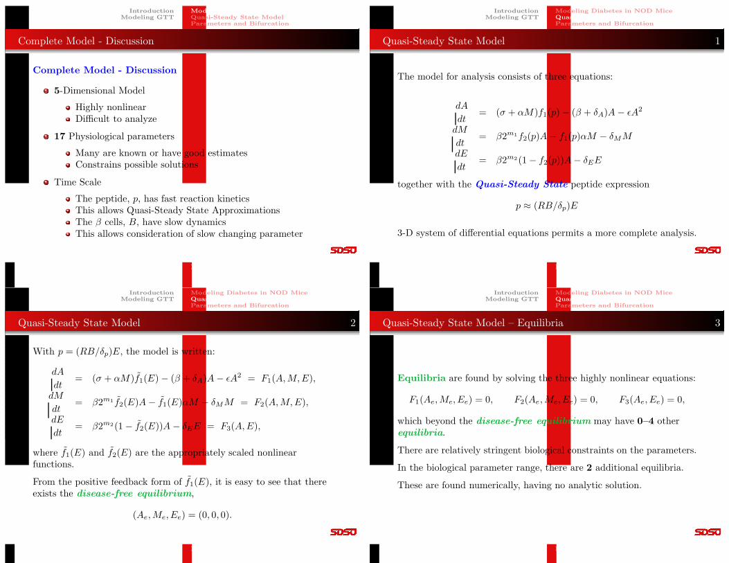
Complete Model - Discussion

Complete Model - Discussion

5-Dimensional Model

Highly nonlinearDifficult to analyze

17 Physiological parameters

Many are known or have good estimatesConstrains possible solutions

Time Scale

The peptide, p, has fast reaction kineticsThis allows Quasi-Steady State ApproximationsThe β cells, B, have slow dynamicsThis allows consideration of slow changing parameter





Quasi-Steady State Model 1

The model for analysis consists of three equations:

dA

dt= (σ + αM)f1(p)− (β + δA)A− ǫA2

dM

dt= β2m1f2(p)A − f1(p)αM − δMM

dE

dt= β2m2(1− f2(p))A− δEE

together with the Quasi-Steady State peptide expression

p ≈ (RB/δp)E

3-D system of differential equations permits a more complete analysis.





Quasi-Steady State Model 2

With p = (RB/δp)E, the model is written:

dA

dt= (σ + αM)f1(E)− (β + δA)A− ǫA2 = F1(A,M,E),

dM

dt= β2m1 f2(E)A− f1(E)αM − δMM = F2(A,M,E),

dE

dt= β2m2(1− f2(E))A − δEE = F3(A,E),

where f1(E) and f2(E) are the appropriately scaled nonlinearfunctions.

From the positive feedback form of f1(E), it is easy to see that thereexists the disease-free equilibrium,

(Ae,Me, Ee) = (0, 0, 0).





Quasi-Steady State Model – Equilibria 3

Equilibria are found by solving the three highly nonlinear equations:

F1(Ae,Me, Ee) = 0, F2(Ae,Me, Ee) = 0, F3(Ae, Ee) = 0,

which beyond the disease-free equilibrium may have 0–4 otherequilibria.

There are relatively stringent biological constraints on the parameters.

In the biological parameter range, there are 2 additional equilibria.

These are found numerically, having no analytic solution.





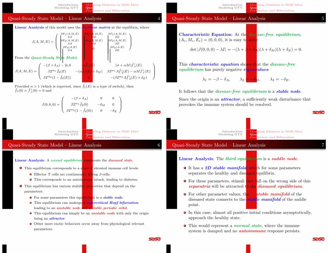
Quasi-Steady State Model – Linear Analysis 4

Linear Analysis of this model uses the Jacobian matrix at the equilibria, where

J(A,M,E) =

∂F1(A,M,E)∂A

∂F1(A,M,E)∂M

∂F1(A,M,E)∂E

∂F2(A,M,E)∂A

∂F2(A,M,E)∂M

∂F2(A,M,E)∂E

∂F3(A,E)∂A

0∂F3(A,E)

∂E

From the Quasi-Steady State Model,

J(A,M,E) =

−(β + δA)− 2ǫA αf1(E) (σ + αM)f ′1(E)

β2m1 f2(E) −(αf1(E) + δM ) β2m1Af ′2(E)− αMf ′

1(E)

β2m2 (1− f2(E)) 0 −(β2m2Af ′2(E) + δE)

Provided n > 1 (which is expected, since f1(E) is a type of switch), thenf1(0) = f ′

1(0) = 0 and

J(0, 0, 0) =

−(β + δA) 0 0

β2m1 f2(0) −δM 0

β2m2 (1 − f2(0)) 0 −δE






Characteristic Equation: At the disease-free equilibrium,(Ae,Me, Ee) = (0, 0, 0), it is easy to solve

det |J(0, 0, 0)− λI| = −(λ+ β + δA)(λ+ δM )(λ+ δE) = 0.

This characteristic equation shows that the disease-freeequilibrium has purely negative eigenvalues:

λ1 = −β − δA, λ2 = −δM , λ3 = −δE.

It follows that the disease-free equilibrium is a stable node.

Since the origin is an attractor, a sufficiently weak disturbance thatprovokes the immune system should be resolved.






Linear Analysis: A second equilibrium represents the diseased state.

This equilibrium corresponds to a state of elevated immune cell levels.

Effector T cells are continuously killing β-cells.

This corresponds to an autoimmune attack, leading to diabetes.

This equilibrium has various stability properties that depend on the

parameters.

For some parameters this equilibrium is a stable node.

This equilibrium can undergo a supercritical Hopf bifurcation

leading to an unstable node and a stable periodic orbit.

This equilibrium can simply be an unstable node with only the origin

being an attractor.

Other more exotic behaviors occur away from physiological relevant

parameters.






Linear Analysis: The third equilibrium is a saddle node.

It has a 2D stable manifold, which for some parametersseparates the healthy and diseased equilibria.

For these parameters, stimuli that fall on the wrong side of thisseparatrix will be attracted to the diseased equilibrium.

For other parameter values, the unstable manifold of thediseased state connects to the stable manifold of the saddlepoint.

In this case, almost all positive initial conditions asymptotically,approach the healthy state.

This would represent a normal state, where the immunesystem is damped and no autoimmune response persists.





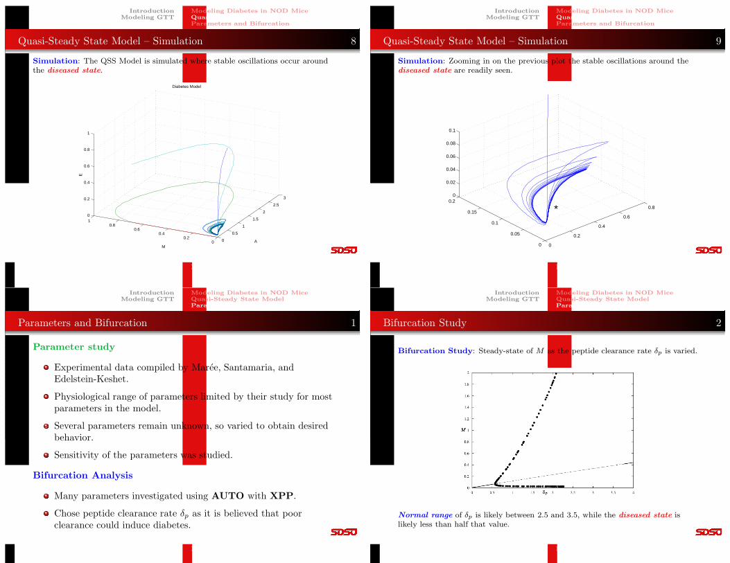
Quasi-Steady State Model – Simulation 8

Simulation: The QSS Model is simulated where stable oscillations occur aroundthe diseased state.

0

0.5

1

1.5

2

2.5

3

00.2

0.40.6

0.810

0.2

0.4

0.6

0.8

1

A

Diabetes Model

M

E





Quasi-Steady State Model – Simulation 9

Simulation: Zooming in on the previous plot the stable oscillations around thediseased state are readily seen.

0

0.2

0.4

0.6

0.8

0

0.05

0.1

0.15

0.20

0.02

0.04

0.06

0.08

0.1

*





Parameters and Bifurcation 1

Parameter study

Experimental data compiled by Maree, Santamaria, andEdelstein-Keshet.

Physiological range of parameters limited by their study for mostparameters in the model.

Several parameters remain unknown, so varied to obtain desiredbehavior.

Sensitivity of the parameters was studied.

Bifurcation Analysis

Many parameters investigated using AUTO with XPP.

Chose peptide clearance rate δp as it is believed that poorclearance could induce diabetes.





Bifurcation Study 2

Bifurcation Study: Steady-state of M as the peptide clearance rate δp is varied.

Normal range of δp is likely between 2.5 and 3.5, while the diseased state islikely less than half that value.





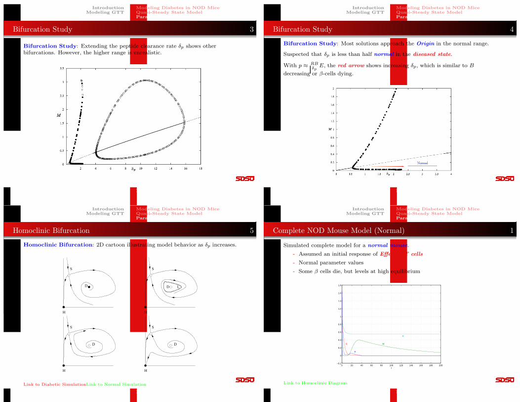
Bifurcation Study 3

Bifurcation Study: Extending the peptide clearance rate δp shows otherbifurcations. However, the higher range is unrealistic.





Bifurcation Study 4

Bifurcation Study: Most solutions approach the Origin in the normal range.

Suspected that δp is less than half normal in the diseased state.

With p ≈RBδp

E, the red arrow shows increasing δp, which is similar to B

decreasing or β-cells dying.





Homoclinic Bifurcation 5

Homoclinic Bifurcation: 2D cartoon illustrating model behavior as δp increases.

S

H

D L

H

S

D

D

H

S

D

H

S

Link to Diabetic SimulationLink to Normal Simulation





Complete NOD Mouse Model (Normal) 1

Simulated complete model for a normal mouse.

- Assumed an initial response of Effector T cells

- Normal parameter values

- Some β cells die, but levels at high equilibrium

0 20 40 60 80 100 120 140 160 180 200−0.2

0

0.2

0.4

0.6

0.8

1

1.2

1.4

1.6

1.8

t

A

E M

B

Link to Homoclinic Diagram





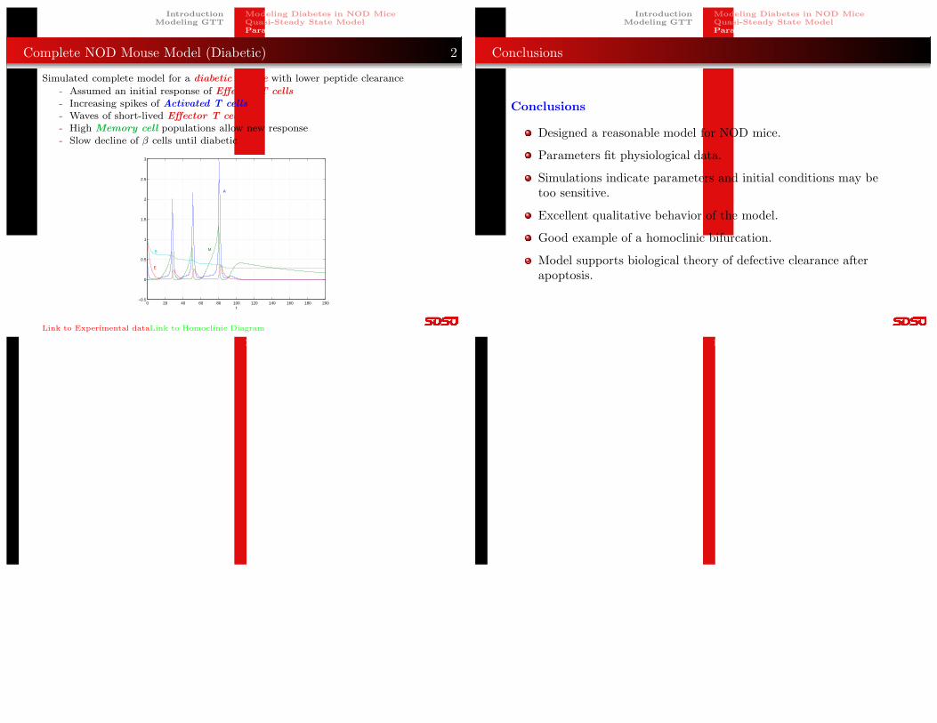
Complete NOD Mouse Model (Diabetic) 2

Simulated complete model for a diabetic mouse with lower peptide clearance

- Assumed an initial response of Effector T cells- Increasing spikes of Activated T cells- Waves of short-lived Effector T cells- High Memory cell populations allow new response- Slow decline of β cells until diabetic

0 20 40 60 80 100 120 140 160 180 200−0.5

0

0.5

1

1.5

2

2.5

3

t

A

E

MB

Link to Experimental dataLink to Homoclinic Diagram





Conclusions

Conclusions

Designed a reasonable model for NOD mice.

Parameters fit physiological data.

Simulations indicate parameters and initial conditions may betoo sensitive.

Excellent qualitative behavior of the model.

Good example of a homoclinic bifurcation.

Model supports biological theory of defective clearance afterapoptosis.


Math 636 - Mathematical Modeling - Modeling Diabetes

Documents

Transcript of Math 636 - Mathematical Modeling - Modeling Diabetes