Math 636 - Mathematical Modeling - Age-Structured...

Age-Structured ModelIntroduction - Hematopoiesis

Model for ErythropoiesisThrombopoiesis

Math 636 - Mathematical Modeling

Age-Structured Models

Joseph M. Mahaffy,〈[email protected]〉

Department of Mathematics and StatisticsDynamical Systems Group

Computational Sciences Research Center

San Diego State UniversitySan Diego, CA 92182-7720

http://jmahaffy.sdsu.edu

Fall 2018

Joseph M. Mahaffy, 〈[email protected]〉 Age-Structured Models — (1/82)

http://jmahaffy.sdsu.edu



Outline

1 Age-Structured ModelMethod of CharacteristicsBirth Boundary ConditionExample

2 Introduction - Hematopoiesis

3 Model for ErythropoiesisMethod of CharacteristicsModel for Erythropoiesis with DelaysAnalysis of DDE with 1-delayAnalysis of Erythropoiesis Model

4 ThrombopoiesisModel for ThrombopoiesisCyclical ThrombocytopeniaAnalysis2-Delay Aside




Introduction

Introduction

Discrete models for total population at discrete times tn:

Pn+1 = f(tn, Pn).

Continuous models for total populations, using ODEs:

dP

dt= f(t, P ).

Leslie model divided population into discrete age classes:

Pn+1 = LPn.

Continuous PDE model, p(t, a):

Allow the population to vary in both time t and age a.Model described by a PDE.Dynamics better describe population, but harder to followfrom complexities of analysis.




Method of CharacteristicsBirth Boundary ConditionExample

Age-Structured Model

Age-Structured Model: Modeling with a hyperbolic PDE.

Mathematical modeling of populations often needs informationabout the ages of the individuals in the population.

This modeling approach was developed primarily by McKendrick(1926) and Von Foerster (1959).

Key Elements in Model

Let n(t, a) denote the population at time t and age a.The birth rate of individuals b(a) depends on the age ofthe adult population.Similarly, the death rate of individuals µ(a) depends onthe age of the individuals.Must specify the initial age distribution of thepopulation, f(a).





Age-Structured Population

Age-Structured Population: Consider a population, n(t, a),dependent on time, t, and structured by age of individuals, a.

The dynamics in time must satisfy:

d

dtn(t, a) =

∂n

∂t+

da

dt

∂n

∂a,

by the chain rule.

Most commonly, the age clocks along with time, so dadt

= 1, so itfollows that

d

dtn(t, a) =

∂n

∂t+

∂n

∂a.

The births all occur at a = 0 (the boundary), so the dynamics of thepopulation above is only deaths or

∂n

∂t+

∂n

∂a= −g(t, a, n).






Age-Structured Model: The McKendrick-Von Foerster equation is:

∂n

∂t+

∂n

∂a+ µ(a)n(t, a) = 0,

with the birth boundary condition (Malthusian):

n(t, 0) =

∫ ∞

0b(a)n(t, a) da,

and the initial condition:n(0, a) = f(a).

b(a)

a

Birth Function

a

µ(a)

Death Function






Discussion for the Age-Structured Model

∂n

∂t+

∂n

∂a= −µ(a)n(t, a).

The PDE shows that age advances with time.

The right side shows that there is only a loss of population through deathwith death increasingly likely with age.

The birth function:

Young individuals are incapable of giving birthThe birth function increases to peak fertility.Births are Malthusian - proportional to the population.After peak fertility, reproductive ability decreases, and itcould again decrease to zero.

The initial population distribution could be anything

However, in general the population distribution should decrease withincreasing time.





Age-Structured Model - Method of Characteristics

t

an(t,0)

n(0, a)

a>t

a<t

The Age-Structured Model:

∂n

∂t+

∂n

∂a= −µ(a)n(t, a).

can be written as an ODE:

d

dtn(t, a) = −µ(a)n(t, a),

along the characteristic,

a(t) = t+ c.

This has the solution:

N(t) = N0 e−

∫

t

0µ(s) ds,

which follows the population of a particular age cohort.





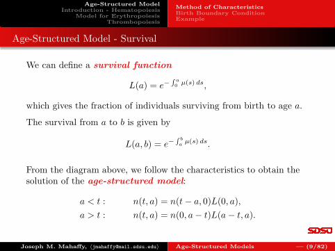
Age-Structured Model - Survival

We can define a survival function

L(a) = e−∫

a

0µ(s) ds,

which gives the fraction of individuals surviving from birth to age a.

The survival from a to b is given by

L(a, b) = e−∫

b

aµ(s) ds.

From the diagram above, we follow the characteristics to obtain thesolution of the age-structured model:

a < t : n(t, a) = n(t− a, 0)L(0, a),

a > t : n(t, a) = n(0, a− t)L(a− t, a).






The age-structured model gives the dynamics of a particular agecohort following a characteristic.

The long term behavior depends significantly on the birth processon the boundary.

Since this is a type of Malthusian growth (with no limitingnonlinearities), we expect a type of exponential growth (ordecline) with some rate r and having the form:

n(t, a) = Cn∗(a)ert,

where n∗(a) is the stable age distribution and C depends on theinitial conditions.

For convenience, assume n∗(0) = 1, so that n∗(a) is the fraction of agea individuals surviving to age a relative to age 0.





Age-Structure Model - Birth Function

The boundary condition of births is

n(t, 0) =

∫

∞

0

b(a)n(t− a, 0)L(a) da.

Inserting the assumed stable form, n(t, a) = Cn∗(a)ert, gives

Cert =

∫

∞

0

b(a)Cer(t−a)L(a) da,

1 =

∫

∞

0

e−raL(a)b(a) da.

Whether r is positive or negative determines if the overall populationgrows or decays.

If r > 0, then the total population grows like Cert





Age-Structure Model - R0

Ecologists and epidemiologists define an important constant R0,which is used to determine if a population (or disease) expands orcontracts.

For this population, define

R0 =

∫

∞

0

L(a)b(a) da,

where R0 represents the average number of (female) offspring from anindividual (female) over her lifetime (integral of births times lifespan).

Note that if R0 < 1, then r < 0 and if R0 > 1, then r > 0. The lattercondition indicates that each female during her lifetime must producemore than one female offspring for the population to grow.

Since n(t, a) = n(t− a, 0)L(a), the stable age distribution satisfies

Certn∗(a) = Cer(t−a)n∗(0)L(a) = Cer(t−a)L(a),

n∗(a) = e−raL(a).





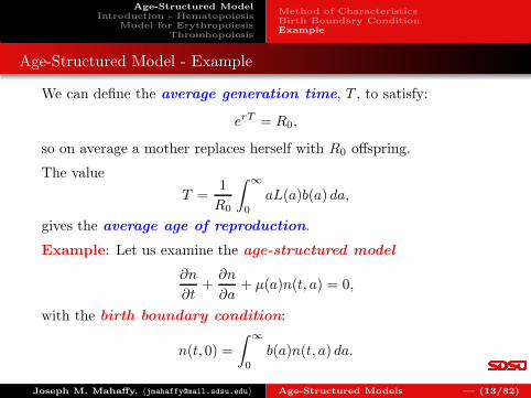
Age-Structured Model - Example

We can define the average generation time, T , to satisfy:

erT = R0,

so on average a mother replaces herself with R0 offspring.

The value

T =1

R0

∫

∞

0

aL(a)b(a) da,

gives the average age of reproduction.

Example: Let us examine the age-structured model

∂n

∂t+

∂n

∂a+ µ(a)n(t, a) = 0,

with the birth boundary condition:

n(t, 0) =

∫

∞

0

b(a)n(t, a) da.






In order to perform calculations (with the help of Maple), we take birth anddeath functions

b(a) =

{

0.3, 3 < a < 8,0, otherwise,

and µ(a) = 0.02 e0.25a.

The birth function assumes a constant fecundity of 0.3 between the ages of 3 and8, while the death function assumes an ever increasing function with age.

0 5 10 150

0.1

0.2

0.3

0.4

0.5

0.6

0.7

0.8

0.9

1

b(a)

a

Birth Function

0 5 10 150

0.1

0.2

0.3

0.4

0.5

0.6

0.7

0.8

0.9

1

µ(a)

a

Death Function

Note: These functions are very crude approximations to the forms displayedearlier.






The age-structured model had a survival function

L(a) = e−∫

a

0µ(s) ds = e−0.08(e0.25a−1),

which gives the fraction of individuals surviving from birth to age a.

0 5 10 15 200

0.1

0.2

0.3

0.4

0.5

0.6

0.7

0.8

0.9

1

L(a)

a

Cohort Survival






The basic reproduction number, R0, was given by

R0 =

∫ ∞

0L(a)b(a) da =

∫ 8

30.3e−0.08(e0.25a−1)da = 1.1678,

which is the average number of (female) offspring from an individual (female) overher lifetime.

With the help of Maple, we can determine the average overall growth rate, r, forthis example.

Maple solves the equation for r:

1 =

∫ ∞

0e−raL(a)b(a) da =

∫ 8

30.3e−rae−0.08(e0.25a−1)da,

and obtainsr = 0.02925985.

This shows the overall population is growing about 3% per unit time.






The Malthusian growth would not be sustainable over long periods of time, sononlinear terms for crowding and other factors would need to be included in themodel, e.g., logistic growth.

With the overall population growth rate, we can obtain the steady-state agedistribution of this population:

n∗(a) = e−raL(a) = e−0.02926ae−0.08(e0.25a−1).

0 5 10 15 200

0.1

0.2

0.3

0.4

0.5

0.6

0.7

0.8

0.9

1

e−raL(a)

a

Stable Age Distribution






The average generation time, T , satisfies:

erT = R0 or e0.02926T = 1.1678.

so on average a mother replaces herself with R0 offspring inT = 5.3024 time units.

The value,

T =1

R0

∫

∞

0

aL(a)b(a) da =1

1.1678

∫ 8

3

0.3a e−0.08(e0.25a−1)da = 5.33205,

gives the average age of reproduction.

In summary, the method of characteristics allows solutions for theage-structured model, which can provide interesting informationabout the behavior of a population.

Needless to say, these models must be significantly expanded tomanage more realistic populations, which in turn significantlycomplicates the mathematical analysis.




Introduction - Hematopoiesis

Hematopoiesis for Erythrocytes and Platelets

All cells in bloodline begin as undifferentiated stem cells (MultipotentialHematopoietic Stem Cells)

Different hormonal signals cause differentiation (Common MyeloidProgenitor (CMP))

Further signals for differentiation

Erythropoiesis – Proerythroblast

Thrombopoiesis – Megakaryoblast

Proliferation via cell doubling

Specialization

Erythropoiesis – Reticulocytes with hemoglobin

Thrombopoiesis – Endomitosis forming Megakaryocytes

Maturation producing Erythrocytes and Platelets

Cell number and volume monitored by body with negative feedback –Erythropoietin and Thrombopoietin




Diagram for Hematopoiesis




Method of CharacteristicsModel for Erythropoiesis with DelaysAnalysis of DDE with 1-delayAnalysis of Erythropoiesis Model

Erythropoiesis

Erythropoiesis is the process for producing Erythrocytes or RedBlood Cells (RBCs).

RBCs are the most numerous cells that we produce in ourbodies, accounting for almost 85% by numbers.

Critical for carrying O2 to our other cells, using the proteinhemoglobin (Hb).

By volume, RBCs are about 40% of blood (∼ 3% body wt).





Erythropoiesis

Erythrocytes or Red Blood Cells

RBCs begin from undifferentiated stem cells (multipotentprogenitors), then based on erythropoietin (EPO) levelsmultiply and specialize.

The body senses O2 levels in the body and releaseserythropoietin (EPO) inversely to the O2 in the blood(negative feedback).

Progenitor cells specialize though a series of cell divisions andintracellular changes (taking about 6 days), buildinghemoglobin (Hb) levels and becoming RBCs.

RBCs circulate in the bloodstream for about 120 days, then areactively degraded.





Model for Erythropoiesis

Age-Structured Model for Erythropoiesis

S0(E) p(t,µ)

∂p

∂t+ V (E) ∂p

∂µ= β(µ, E)p

V (E) −→

m(t, ν)

⊖

⊕

⊕

∂m∂t

+ ∂m∂ν

= −γ(ν)m

E(t)E = a

1+KM r − kE

M(t) =∫ νF0 m(t, ν)dν

0 µ1 µF 0 νF






Age-Structured Model viewed as a conveyor system





Active Degradation of RBCs

Active Degradation of RBCs

RBCs are lost from normal leakage (breaking capillaries), whichis simply proportional to the circulating numbers

RBCs age - Cell membrane breaks down (no nucleus to repair)from squeezing through capillaries

Aged membrane is marked with antibodies

Macrophages destroy least pliable cells based on the antibodymarkers

Model assumes constant supply macrophages

Saturated consumption of Erythrocytes

- Satiated predator eating a constant amount per unit timeConstant flux of RBCs being destroyed





Constant Flux Boundary Condition


Let Q be rate of removal of erythrocytes

Erythrocytes lost are Q∆t

Mean Value Theorem - average number RBCs

m(ξ, νF (ξ)) for ξ ∈ (t, t+∆t)

Balance law

Q∆t = W∆t m(ξ, νF (ξ))

−[νF (t+∆t)− νF (t)]m(ξ, νF (ξ))

As ∆t → 0,Q = [W − νF (t)]m(t, νF (t))






If macrophages consume a constant amount of RBCs at the endof their, we obtain the natural BC

Q = [W − νF (t)]m(t, νF (t))

This results in the lifespan of the RBCs either lengthening orshortening from the normal 120 days

This implies that the lifespan of the RBCs depends on the stateof the system





Model Reduction

Model Reduction: Several simplifying assumptions are made:

Assume that both velocities of aging go with time, t,

V (E) = W = 1.

Assume the birth rate β satisfies:

β(µ,E) =

{

β, µ < µ1,

0, µ ≥ µ1,

Assume that γ is constant.

The model satisfies the age-structured partial differentialequations:

∂p

∂t+

∂p

∂µ= β(µ)p,

∂m

∂t+

∂m

∂ν= −γm.






The boundary conditions for the age-structured PDEs are:

Recruitment of the precursors based on EPO concentration circulating inthe blood:

p(t, 0) = S0(E).

Continuity of precursors maturing and entering the bloodstream as matureRBCs:

p(t, µF ) = m(t, 0).

Active destruction of mature RBCs:

(1− νF (t))m(t, νF (t)) = Q.

The negative feedback by EPO satisfies the ODE:

E =a

1 +KMr− kE,

where the total mature erythrocyte population is

M(t) =

∫ νF (t)

0m(t, ν)dν.





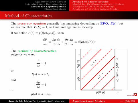
Method of Characteristics

The precursor equation generally has maturing depending on EPO, E(t), butwe assume that V (E) = 1, so time and age are in lockstep.

If we define P (s) = p(t(s), µ(s)), then

dP

ds=

∂p

∂t

dt

ds+

∂p

∂µ

dµ

ds= β(µ(s))P (s).

t

µ

p(t,0)=

S0(E

)

p(t,µF)=

m(t,0)

p(0,µ)

µ>t

µ<t

The method of characteristicssuggests we want

dt

ds= 1

ort(s) = s+ t0,

anddµ

ds= 1

orµ(s) = s+ µ0.






With the method of characteristics, the precursor equation,

dP

ds= β(µ(s))P (s),

is a birth only population model.

The model assumes that the body uses apoptosis at the earlyrecruitment stage (CFU-E) to decide how many precursor cells areallowed to mature.

The solution to the ODE above is

P (s) = p(t, µ) = P (0)e∫

s

0β(µ(r))dr,

which is valid for 0 < µ < µF , focusing on the larger time solution.






This aging process of the precursor cells is primarily a time of amplification innumbers before the final stages of simply add hemoglobin.

The model shows how recruited cells amplify, then enter the maturecompartment (bloodstream) to circulate and carry O2:

p(t, µF ) = p(t0, 0)e∫ s0 β(µ(r))dr

= p(t− µF , 0)eβµ1 = eβµ1S0(E(t− µF )).

From the method of characteristics on the mature RBCs, a similar result gives:

m(t, ν) = m(t − ν, 0)e−γν .

The continuity between the precursors and the mature RBCs gives:

m(t − ν, 0) = p(t− ν, µF ) = eβµ1S0(E(t − µF − ν)).





Total RBCs

The O2 carrying capacity of the body depends on the total number of RBCs,which is the integral over all m(t, ν) in ν:

M(t) =

∫ νF (t)

0m(t − ν, 0)e−γνdν

=

∫ νF (t)

0eβµ1S0(E(t− µF − ν))e−γνdν,

= e−γ(t−µF )eβµ1

∫ t−µF

t−µF−νF (t)S0(E(w))eγwdw.

We apply Leibnitz’s rule for differentiating an integral:

M(t) = −γe−γ(t−µF )eβµ1

∫ t−µF

t−µF−νF (t)S0(E(w))eγwdw,

+eβµ1

[

S0(E(t − µF ))− S0(E(t − µF − νF (t)))e−γνF (t)(1 − νF (t))]

= −γM(t) + eβµ1S0(E(t − µF )) −Q,





Model for Erythropoiesis with Delays

After reduction of PDEs, the state variables become total matureerythrocytes, M , EPO, E, and age of RBCs, νF .

dM(t)

dt= eβµ1S0(E(t− µF ))− γM(t)−Q

dE(t)

dt= f(M(t))− kE(t)

dνF (t)

dt= 1−

Qe−βµ1eγνF (t)

S0(E(t− µF − νF (t)))

This is a state-dependent delay differential equation.





Model for Erythropoiesis with Delays

Properties of the Model: Integrating along the characteristicsshows that the maturation process acts like a delay, changing theage-structured model into a delay differential equation.

The state-dependent delay model has a unique positiveequilibrium.

The delay µF accounts for maturing time.

The state-dependent delay in equation for νF (t) comes fromthe varying age of mature cells.

The νF (t) differential equation is uncoupled from the differentialequations for M and E.

Stability is determined by equations for M and E





DDE with One Delay

Consider the delay differential equation (DDE) with one delay:

y(t) = ay(t) + by(t − r)

If one tries the solution, y(t) = ceλt, then

cλeλt = aceλt + bceλ(t−r),

which gives the characteristic equation

λ− a = be−λr

The boundary of stability is a subset of solutions to the characteristic equationwith λ = iω or

iω − a = be−iωr = b (cos(ωr) − i sin(ωr)) ,

or for λ = 0, the real root crossing satisfies:

a = −b.





DDE with One Delay

From the characteristic equation with λ = iω, the real andimaginary parts give the parametric equations:

a(ω) = −b(ω) cos(ωr),

ω = −b(ω) sin(ωr).

Solving these equations for a(ω) and b(ω) gives

a(ω) = ω cot(ωr),

b(ω) = −ω

sin(ωr),

which are clearly singular at any nπr, n = 0, 1, ...

This creates distinct curves ω ∈(

(n−1)πr

, nπr

)

for n = 1, 2, ...





Stability Region - DDE with One Delay

−10 −8 −6 −4 −2 0 2 4 6 8 10−10

−8

−6

−4

−2

0

2

4

6

8

10Stability Region

Stable Region

(1/r, −1/r)

a

b

Real root crossing solid blue line (λ = 0 with a = −b).

“Hopf bifurcation” crossing solid red line.

Curves above create a D-partitioning of the complex plane into distinctregions with distinct integer number of eigenvalues with real positive parts.





Comments DDE with One Delay

The characteristic equation of a delay differential equation (DDE) is anexponential polynomial, which can rarely be solved exactly.

Stability of the DDE is demonstrated by showing all roots (infinite) have negativereal parts.

The analysis above finds the stability region for the DDE

y(t) = ay(t) + by(t − r)

Region with a < 0 and |b| < |a| is stable independent of the delay

As r → 0, the DDE approaches the ODE with stability region a+ b < 0

Stability region comes to a point at(

1r,− 1

r

)

Imaginary root crossings are distinct, non-intersecting curves, leaving thisstability boundary generated by the parametric equations with ω ∈

(

0, πr

)

.





Argument Principle

The Argument Principle from complex variables is one techniquefor locating the eigenvalues.

Theorem (Argument Principle)

If f(z) is a meromorphic function inside and on some closed

contour C, with f having no zeros or poles on C, then the following

formula holds:∮

C

f ′(z)

f(z)dz = 2πi(N − P ),

where N and P denote respectively the number of zeros and poles of

f(z) inside the contour C, with each zero and pole counted as many

times as its multiplicity and order, respectively. This assumes that the

contour C is simple and is oriented counter-clockwise.





Argument Principle: Stability Analysis

Since the characteristic equation, f(λ), is an analytic function, then theArgument Principle finds the zeroes of f(λ).

A geometric method of employing the Argument Principle is to consider acontour, C, (counterclockwise), then create a map f(C) with the analyticfunction, f(λ).

The map f(C) creates a curve in the complex plan, and the ArgumentPrinciple states that this map will encircle the origin N times(counterclockwise), where N is the number of zeroes inside C.

Stability analysis for differential equations with the Argument Principle

(sometimes called Nyquist criterion) uses an appropriate contour in the

right half of complex plane.

For ODEs, create semi-circle radius R with diameter on imaginary

axis, then let R → ∞.

For DDEs, often sufficient to take rectangle from [−πr, πr] on

imaginary axis and real part arbitrarily large.





MatLab Application for ODEs

We want to show stability of examples from ODEs

1 y + y − 6y = 0

- Characteristic equation: λ2 + λ− 6 = 0- Shows 1 encirclements (Unstable)

2 y − 2y + 2y = 0

- Characteristic equation: λ2 − 2λ+ 2 = 0- Shows 2 encirclements (Unstable)

3 y + 2y + 2y = 0

- Characteristic equation: λ2 + 2λ+ 2 = 0- Shows no encirclements (Stable)





Contour

The graph below is the contour to which we apply ourcharacteristic equations.

0 2 4 6 8 10-5

0

5

(p, q)

λ = µ+ iν

µ

ν

>

<<

>





Argument Principle for Polynomial

Consider the polynomial equation

p(λ) = λ2 + aλ + b.

1 function poly (a,b,p,q)2 % Polynomial xˆ2 + ax + b3 % p = x max, q = y max4

5 h=p/100;6 k=q/50;7 x(1) = 0;8 y(1) = q;9 u1(1) = x(1)ˆ2-y(1)ˆ2+a * x(1)+b;

10 w1(1) = 2 * x(1) * y(1)+a * y(1);11 for i=2:10112 x(i) = 0;13 y(i) = y(i-1)-k;14 u1(i) = x(i)ˆ2-y(i)ˆ2+a * x(i)+b;






15 w1(i) = 2 * x(i) * y(i)+a * y(i);16 end17 for i=102:20118 x(i) = x(i-1)+h;19 y(i) = -q;20 u2(i-101) = x(i)ˆ2-y(i)ˆ2+a * x(i)+b;21 w2(i-101) = 2 * x(i) * y(i)+a * y(i);22 end23 for i=202:30124 x(i) = p;25 y(i) = y(i-1)+k;26 u3(i-201) = x(i)ˆ2-y(i)ˆ2+a * x(i)+b;27 w3(i-201) = 2 * x(i) * y(i)+a * y(i);28 end






29 for i=302:40130 x(i) = x(i-1)-h;31 y(i) = q;32 u4(i-301) = x(i)ˆ2-y(i)ˆ2+a * x(i)+b;33 w4(i-301) = 2 * x(i) * y(i)+a * y(i);34 end35 plot (u1,w1, 'b-' ,u2,w2, 'r-' ,u3,w3, 'g-' ,u4,w4, 'm-' ); grid





MatLab Application for DDEs

Eigenvalues for Examples from DDEs

1 y(t) = −y(t)− 3y(t− 1)

- Characteristic equation: λ+ 1 = −3e−λ

- Shows 2 encirclements (Unstable)

2 y(t) = −y(t)− 3y(t− 0.5)

- Characteristic equation: λ+ 1 = −3e−0.5λ

- Shows no encirclements (Stable)

3 y(t) = −y(t) + 6y(t− 1)

- Characteristic equation: λ+ 1 = 6e−λ

- Shows 3 encirclements (Unstable)





Argument Principle for DDE

Consider the characteristic equation

f(λ) = λ− a− b e−rλ.

1 function delay 1abr(a,b,r,p,q)2

3 % One-delay z - a - b * eˆ(-r * z)4 % p = x max, q = y max5

6 h=p/100;7 k=q/50;8 x(1) = 0;9 y(1) = q;

10 u1(1) = x(1)-a-b * exp (-r * x(1)) * cos (r * y(1));11 w1(1) = y(1)+b * exp (-r * x(1)) * sin (r * y(1));12 for i=2:10113 x(i) = 0;14 y(i) = y(i-1)-k;






15 u1(i) = x(i)-a-b * exp (-r * x(i)) * cos (r * y(i));16 w1(i) = y(i)+b * exp (-r * x(i)) * sin (r * y(i));17 end18 for i=102:20119 x(i) = x(i-1)+h;20 y(i) = -q;21 u2(i-101) = x(i)-a-b * exp (-r * x(i)) * cos (r * y(i));22 w2(i-101) = y(i)+b * exp (-r * x(i)) * sin (r * y(i));23 end24 for i=202:30125 x(i) = p;26 y(i) = y(i-1)+k;27 u3(i-201) = x(i)-a-b * exp (-r * x(i)) * cos (r * y(i));28 w3(i-201) = y(i)+b * exp (-r * x(i)) * sin (r * y(i));29 end






30 for i=302:40131 x(i) = x(i-1)-h;32 y(i) = q;33 u4(i-301) = x(i)-a-b * exp (-r * x(i)) * cos (r * y(i));34 w4(i-301) = y(i)+b * exp (-r * x(i)) * sin (r * y(i));35 end36 plot (u1,w1, 'b-' ,u2,w2, 'r-' ,u3,w3, 'g-' ,u4,w4, 'm-' ); grid





Linear Analysis of the Model

Due to the negative control by EPO, it can be shown that thismodel has a unique equilibrium:

(M, E, νF ).

With the change of variables, x1(t) = M(t)− M , x2(t) = E(t)− E,and x3(t) = νF (t)− νF and keeping only the linear terms, we obtainthe linear system:

x1(t) = eβµ1S′

0(E)x2(t− µF )− γx1(t),

x2(t) = f ′(M)x1(t)− kx2(t),

x3(t) =1

Ex2(t− µF − νF )− γx3(t).





Linear Analysis of the Model

Let X(t) = [x1(t), x2(t), x3(t)]T , then the linear system can be

written:

X(t) = A1X(t) +A2X(t− µF ) +A3X(t− µF − νF ),

where

A1 =

−γ 0 0f ′(M ) −k 0

0 0 −γ

, A2 =

0 eβµ1S′0(E) 0

0 0 00 0 0

,

and

A3 =

0 0 00 0 00 1

E0

.

We try solutions of the form X(t) = ξeλt giving:

λIξeλt =[

A1 +A2e−λµF +A3e

−λ(µF+νF )]

ξeλt.





Characteristic Equation

Dividing by eλt results in the eigenvalue equation:

(

A1 +A2e−λµF +A3e

−λ(µF+νF ) − λI)

ξ = 0.

So we must solve

det

∣

∣

∣

∣

∣

∣

∣

∣

−γ − λ eβµ1S′

0(E)e−λµF 0

f ′(M) −k − λ 0

0 1Ee−λ(µF+νF ) −γ − λ

∣

∣

∣

∣

∣

∣

∣

∣

= 0,

which gives the characteristic equation

(λ+ γ)[

(λ+ γ)(λ+ k) + Ae−λµF]

= 0,

where A ≡ −eβµ1S′

0(E)f ′(M) > 0.





Stability Analysis of Delay Model

Stability Analysis of the Delay Model

The characteristic equation is an exponential polynomial givenby

(λ+ γ)

(

(λ+ γ)(λ+ k) + Ae−λµF

)

= 0,

which has one solution λ = −γ.

This shows the stability of the νF equation, which was thestate-dependent portion of the delay model.

Remains to analyze

(λ + γ)(λ+ k) = −Ae−λµF .

The boundary of the stability region occurs at a Hopf bifurcation,where the eigenvalues are λ = iω, purely imaginary.






Properties of the Exponential Polynomial (Characteristic Equation)

(λ+ γ)(λ + k) + Ae−λµF = 0.

The solution of the characteristic equation has infinitely many roots.

Discrete delay model is infinite dimensional as the initial data must be afunction of the history over the longest delay.

The exponential polynomial has a leading pair of eigenvalues and many oftrailing having negative real part (Stable Manifold Theorem).

Analysis of the delay model is easier than the generalized age-structuredmodel.

The models are equivalent under the assumption that V (E) = W = 1.

Stability changes to oscillatory when the leading pair of eigenvalues crossthe imaginary axis, a Hopf bifurcation.






Hopf Bifurcation Analysis

A Hopf bifurcation occurs when λ = iω solves the characteristicequation,

(iω + γ)(iω + k) = −Ae−iωµF .

From complex variables, we match the magnitudes:

|(iω + γ)(iω + k)| = A,

where the left side is monotonically increasing in ω, and thearguments

Θ(ω) ≡ arctan

(

ω

γ

)

+ arctan(ω

k

)

= π − ωµF ,

which has infinitely many solutions.

Solve for ω by varying parameters such as γ or µF .





Argument Principle

Hopf Bifurcation: One significant method for finding the roots ofthe characteristic equation at a Hopf bifurcation is the Argument

Principle from complex variables.





Experiments and Model

Experiment:

Give rabbits regularantibodies to RBCs.

This increases destructionrate γ.

Observe oscillationsin RBCs.

Model undergoesHopf bifurcation

with increasing γ.






Model can reasonably match the rabbit data by fitting parametersthat are reasonable.

The model stabilizes with variable velocity, V (E), but a morecomplicated model.




Model for ThrombopoiesisCyclical ThrombocytopeniaAnalysis2-Delay Aside

Thrombopoiesis

Megakaryocytes Platelets

Thrombopoiesis is the process for producing Thrombocytes orPlatelets.

Platelets are about 20% the size of RBCs and there are onlyabout 10-20% by numbers compared to RBCs.

They are critical for repairing damage to blood vessels byclumping together and creating clots.

The half-life for platelets is significantly lower and results in avery high turnover.





Thrombopoiesis

Thrombocytes or Platelets

Platelets begin from undifferentiated stem cells (multipotentprogenitors), and based on thrombopoietin (TPO) levelsmultiply then stop dividing and undergo endomitosis, formingmegakaryocytes (2-256 nuclei).

Thrombopoietin (TPO) is produced constantly then absorbedby megakaryocytes and platelets (negative feedback).

Maturation takes 10-14 days, then megakaryocytes protrudefilopodia into blood vessels and platelets are released.

Platelets circulate in the bloodstream for about 10 days, thenare actively degraded.

TPO circulates at significantly lower concentrations comparedto EPO.





Age-Structured Model for Thrombopoiesis

Age-Structured Model for Thrombopoiesis

Q∗ mx(t, a)

∂mx

∂t+ ∂mx

∂a= ηx(T )mx

ηm(T )ηe(T )

P (t)

⊕

⊕

⊖

⊖

T (t)TprodγTT

Me(t) =∫ τe0 me(t, ν)dν

τm τe

αPF (P )

γPP





Model for ThrombopoiesisModel for Thrombopoiesis

dP

dt=

D0

βP

me (t, τe)− γPP − αPPnP

bnPP + PnP

,

dT

dt= Tprod − γT T − αT (Me (t) + kSβPP )

TnT

knTT + TnT

,

where

me (t, a) = VmκPQ∗ exp

t−a∫

t−a−τm

ηm (T (s)) ds

exp

t∫

t−a

ηe (T (s)) ds

,

Me (t) =

τe∫

0

me (t, a) da.

ηm (T (t)) = ηminm +

(

ηmaxm − ηmin

m

) Tnm

bnmm + Tnm

,

ηe (T (t)) = ηmine +

(

ηmaxe − ηmin

e

) Tne

bnee + Tne

.Joseph M. Mahaffy, 〈[email protected]〉 Age-Structured Models — (63/82)




Notes on Model for Thrombopoiesis

Notes on Model for Thrombopoiesis

The thrombopoiesis model is more complex with many moreparameters than the erythropoiesis model.

The Functional differential equation form is substantiallymore complex, especially the 2 delays of maturation (ηm andηe).

Age-structure reductions are very similar.

The negative feedbacks differ significantly.

Simulations show clear Hopf bifurcations.

Linear analysis is significantly more difficult.





Parameters for Model for Thrombopoiesis

Parameters for Model for Thrombopoiesis

Over 20 parameters in model.

Extensive literature search

Identify some directly.Fit many with existing experimental data.Insufficient sensitivity analysis at this time.

Found asymptotically stable equilibrium for normal subject.

Could vary several parameters (4) to match diseased patients.





Cyclical Thrombocytopenia

Cyclical Thrombocytopenia

Rare, but dangerous pathological state, with very high and lowplatelet counts oscillating with about a month period.

Source of the disease is unknown, but suspect defectiveperipheral control – No good treatment to date.





Unique Equilibrium

From before, we have the Thrombopoiesis Model:

dP

dt=

D0

βP

me (t, τe)− γPP − αP

PnP

bnP

P + PnP,

dT

dt= Tprod − γTT − αT (Me (t) + kSβPP )

T nT

knT

T + T nT,

where the functions me(t, τe) and Me(t) are defined as before.

Theorem (Unique Equilibrium)

The Thrombopoiesis Model has a unique positive equilibrium,

(P ∗, T ∗).

Proof: The proof of this result uses the monotonicity of the functionscomposing the right hand sides of this system of DEs. It is a highlynonlinear system, but the positive and negative feedbacks combine togive a unique equilibrium.





Linearization

Let x(t) = P (t)− P ∗ and y(t) = T (t) − T ∗ and ignore higher order terms, thenthe linearized system becomes:

dx

dt= A2

[

∂T ηm(T ∗)

∫ t−τe

t−τe−τm

y(s) ds+ ∂T ηe(T∗)

∫ t

t−τe

y(s) ds

]

−(

γP + ∂PF (P ∗))

x,

dy

dt= − αT kSβPG(T ∗)x−

(

γT + αT (A1E1 + kSβPP ∗)∂TG(T ∗))

y

− αTA1G(T ∗)

(

∂T ηm(T ∗)

∫ τe

0eηe(T

∗)a

(∫ t−a

t−a−τm

y(s) ds

)

da

+ ∂T ηe(T∗)

∫ τe

0eηe(T

∗)a

(∫ t

t−a

y(s) ds

)

da

)

,

where

A2 =D0VmκP Q∗

βP

eηm(T∗)τm+ηe(T∗)τe , A1 = VmκP Q

∗

eηm(T∗)τm , E1 =

eηe(T∗)τe − 1

ηe(T∗).





Characteristic Equation 1

With solutions of the form [x(t), y(t)]T = [c1, c2]T eλt, the linear functionalequation becomes:

λI

(

c1c2

)

=

(

−L1 L2(λ)−L3 −L4(λ)

)(

c1c2

)

.

The coefficients L1, L2, L3, and L4 are given by

L1 = γP + ∂PF (P∗

),

L2(λ) =A2

λ

[

∂T ηm(T∗

)e−λτe

(

1 − e−λτm

)

+ ∂T ηe(T∗

)(

1 − e−λτe

)]

,

L3 = αT kSβPG(T∗

),

L4(λ) = C1 +C2

λ

[

∂T ηm(T∗

)(

1 − e−λτm

)

(

1 − e−(λ−ηe(T∗))τe)

(λ − ηe(T∗))

+ ∂T ηe(T∗

)

eηe(T∗)τe − 1

ηe(T∗)+

e−(λ−ηe(T∗))τe − 1

λ − ηe(T∗)

]

,





Characteristic Equation 2

From the definitions above the Characteristic Equation becomes:

det

∣

∣

∣

∣

−L1 − λ L2(λ)L3 −L4(λ)− λ

∣

∣

∣

∣

= (λ+ L1)(λ+ L4(λ)) − L2(λ)L3 = 0.

Eliminating the λ terms in the denominator leaves a complicatedexponential polynomial of the form:

P4(λ) + (α1λ+ α0)e−λτm + (β1λ+ β0)e

−λτe + (γ1λ+ γ0)e−λ(τe+τm) = 0.

We have failed to obtain any analytic intuition on this exponential

polynomial, but it is readily solved numerically in Maple and

MatLab.





Numerical Hopf Bifurcation 1

Numerical Hopf Bifurcation

As noted earlier, parameters were fit for a normal subject.

Leading eigenvalues were λ1 ≈ −0.059± 0.053i, which hasthe wrong frequency for observed diseased individuals.The second set of eigenvalues were λ2 ≈ −0.114± 0.359i.λ2 has appropriate frequency and connects numerically toall diseased patients studied.

Created hyperline in parameter space connecting the 4

parameters varied between normal subject and each diseasedpatient.

Following graphs show variations in the values of the equilibriaand the eigenvalues as the 4 parameters vary continuously.






0 10 20 30 4020

40

60

80

100

120

P*

T*

EquilibriaNormal EquilibriumHopf EquilibriumCT Patient Equilibrium

−0.2 −0.1 0 0.1 0.20.22

0.24

0.26

0.28

0.3

0.32

0.34

0.36

Re(λ)

Im(λ)

EigenvaluesNormal EigenvaluesHopf BifurcationCT Patient Eigenvalues

1.8 1.9 2 2.1

30

31

32

33

34

35

P*

T*

−0.1 −0.08 −0.06 −0.04 −0.02 0

0.255

0.26

0.265

0.27

0.275

Re(λ)

Im(λ)






As the 4 parameters vary linearly, the equilibria and theeigenvalues vary continuously.

However, we observe a cusp-like change in a very small region ofthe hyperline (rapid transition).

This needs more detailed exploration.

5 10 15 20 25 30 3520

40

60

80

100

120

P*

T*

EquilibriaNormal EquilibriumHopf EquilibriumCT Patient Equilibrium

−0.15 −0.1 −0.05 0 0.05 0.10.2

0.25

0.3

0.35

0.4

Re(λ)

Im(λ)

EigenvaluesNormal EigenvaluesHopf BifurcationCT Patient Eigenvalues





Belair and Mackey Platelet Model

Two-delay Model for Platelets (Belair and Mackey, 1987)

Platelets

Thrombopoietin β( )Pγ

Megakaryocytes

T sTm0 m+ Tage

dP

dt= − γP (t)−γP (t)+β(P (t− Tm))β(P (t− Tm))β(P (t− Tm))−β(P

Production of platelets (β(P ))Linear loss of platelets, (γP )Discounted destruction of platelets (β(P )e−γTs)

Time delays for maturation (Tm) and life expectancy (Ts)





Modified Platelet Model 1

Modified Platelet Model

Examine a modified form:

dP

dt= −γP (t) +

β0θnP (t−R)

θn + Pn(t−R)− f ·

β0θnP (t− 1)

θn + Pn(t− 1)

Scaled time to normalize the larger delay

Chose parameters similar to Belair and Mackey afterscaling

Introduced parameter f , which is different

Wanted a scaling factor, instead of time delay varyingdiscount






dP

dt= −γP (t) +

β0θP (t−R)


β0θP (t− 1)

θn + Pn(t− 1)

50 50.2 50.4 50.6 50.8 51

−10

−5

0

5

10

t

P

Model with Delays near 1/2

R = 1/2R = 0.48R = 0.51

Figure shows stability at R = 12 , but irregular oscillations for delays

nearby






dP

dt= −γP (t) +

β0θP (t−R)


β0θP (t− 1)

θn + Pn(t− 1)

50 50.2 50.4 50.6 50.8 51

−10

−5

0

5

10

t

P

Model with Delays near 1/3

R = 1/3R = 0.318R = 0.34

Figure shows stability at R = 13 , but irregular oscillations for delays

nearby (Same parameters as R = 12 )





Two-Delay Differential Equation

Two-Delay Differential Equation

y(t) +Ay(t) +B y(t− 1) + C y(t−R) = 0

Delay equations are important in modeling

Two-delay problem

E. F. Infante noted an odd stability property observed in atwo delay economic model, rational delays created a largerregion of stabilityMultiple delays are important for biological modelsDeveloped special geometric techniques for analysis of delayequationsJM and T. C. Busken, Regions of stability for a lineardifferential equation with two rationally dependent delays,DCDS A, 35, 4955-4986 (2015)





Stability Regions for Different Delays

Technique creates parametric families of curves from the imageof the imaginary axis

Similarity of limited family types prevent approach of MinimumRegion of Stability (Black dashed lines)

Below shows first 100 parametric curves for A = 1000

−2000 −1000 0 1000 2000−2000

−1500

−1000

−500

0

500

1000

1500

2000R = 0.33333 and A = 1000.00000

B axis

C a

xis

−2000 −1000 0 1000 2000−2000

−1500

−1000

−500

0

500

1000

1500

2000R = 0.45000 and A = 1000.00000

B axis

C a

xis

−2000 −1000 0 1000 2000−2000

−1500

−1000

−500

0

500

1000

1500

2000R = 0.50000 and A = 1000.00000

B axis

C a

xis

R = 13 R = 0.45 R = 1

2






Returning to the modified platelet model

The coefficients of the linearized model are approximately(A,B,C) = (100, 35,−100) (black circle)

Our D-partitioning curves for R = 13 are below

−100 −50 0 50 100

−100

−50

0

50

100

R = 0.33333 and A = 100.00000

B axis

C a

xis

0 10 20 30 40 50 60 70−120

−110

−100

−90

−80

−70

−60

−50R = 0.33333 and A = 100.00000

B axis

C a

xis






The coefficients of the linearized model are approximately(A,B,C) = (100, 35,−100) (black circle)

Our D-partitioning curves for R = 0.318 are below

−100 −50 0 50 100

−100

−50

0

50

100

R = 0.31800 and A = 100.00000

B axis

C a

xis

0 10 20 30 40 50 60 70−120

−110

−100

−90

−80

−70

−60

−50R = 0.31800 and A = 100.00000

B axis

C a

xis





Discussion/Conclusions

Created age-structured models for hematopoiesis

Can fit parameters to experimental data

Reasonably fit normal and diseased patients

Provides some insight to cyclical thrombocytopenia

Remains some sensitivity issues with parameters - startexamining a simpler model

Ultimately want model to give insights into treatments


Math 636 - Mathematical Modeling - Age-Structured...

Documents

Transcript of Math 636 - Mathematical Modeling - Age-Structured...