Markov Chain Methods for Analyzing Urban...

J Stat Phys (2008) 132: 1051–1069DOI 10.1007/s10955-008-9591-2

Markov Chain Methods for Analyzing Urban Networks

D. Volchenkov · P. Blanchard

Received: 18 October 2007 / Accepted: 17 June 2008 / Published online: 16 July 2008© Springer Science+Business Media, LLC 2008

Abstract Complex transport networks abstracted as graphs (undirected, directed, or multi-component) can be effectively analyzed by random walks (or diffusions). We have unifiedmany concepts into one framework and studied in details the structural and spectral proper-ties of spatial graphs for five compact urban patterns.

Keywords Random walks · Complex networks · Traffic equilibrium

1 Introduction

Topology of urban environments can be represented by means of graphs. From Euler’s time,urban design and townscape studies were the sources of inspiration for the network analysisand graph theory.

Transport networks are used to model the flow of commodity, information, viruses, opin-ions, or traffic along roads, streets, pipes, aqueducts, power lines, or nearly any structurewhich permits either the movement of vehicles or the flow of some commodity, products,goods or service. In Sect. 2, we discuss how a transport network may be represented bydifferent graphs in accordance to the object-based, space-based, or time-based paradigms.

In particular, we explore the spatial graph representations of several compact urban pat-terns by random walks. Two of them are situated on islands: Manhattan (with an almostregular grid-like city plan) and the network of Venice canals (Venice stretches across 122small islands, and the canals serve the function of roads). We have also considered two or-ganic cities founded shortly after the Crusades and developed within the medieval fortresses:Rothenburg ob der Tauber (the medieval Bavarian city preserving its original structure fromthe 13th century) and the downtown of Bielefeld (Altstadt Bielefeld), an economic and cul-tural center of Eastern Westphalia. To supplement the study of urban canal networks, wehave investigated that one in the city of Amsterdam.

D. Volchenkov (�) · P. BlanchardBiBoS, University Bielefeld, Postfach 100131, 33501, Bielefeld, Germanye-mail: [email protected]

mailto:[email protected]

1052 D. Volchenkov, P. Blanchard

While identifying a street (canal) over a plurality of routes on the city map, the “named-street” approach had been used, in which two different arcs of the original street (canal)network are assigned to the same street ID provided they have the same street name. Thespatial graphs of the urban patterns have been constructed by mapping edges coded with thesame street (canal) ID into nodes of the spatial graph, and intersections among each pair ofedges in the original graph—into edges connecting the corresponding nodes.

In general, graphs do not possess the structure of Euclidean space and therefore, theirstructural analysis can be difficult. In Sect. 3, we show that a structure of Euclidean spacecan nevertheless be defined on undirected graphs by random walks (or diffusions).

In Sect. 4, we have analyzed the spectral properties of Laplace operator describing thediffusion process on the spatial graphs representing the compact urban patterns and foundthat the spectral densities for them are close to normal distributions.

In Sect. 5, we investigate the Laplace spectra (which are non-negative) by the methodof characteristic functions strongly inspired by statistical mechanics. The mean eigenvalue(which corresponds to the internal energy in statistical mechanics), the standard deviationof eigenvalues around the mean, and the entropy allow tracks out the dramatic structuraldifference between organic cities gradually developed during centuries and modern citiesplanned in grid.

In Sect. 6, we have extended the approach developed in the previous sections to the caseof directed graphs and multi-component directed graphs. The latter graphs can be consideredas a number of transport networks (transportation modes) interacting with each other bymeans of passengers.

We conclude in the last section.

2 Transport Networks and Their Representations

The ultimate goals of network theory are to help people in planning the efficient land use,feasible logistic, expeditious energy grids, and streamlined communications. Most of thelife-sustaining networks are essentially small—usually, they amount to just several hundrednodes connected by no means at random.

Systems consisting of many individual units sharing information, people, and goods haveto be modified frequently to meet the natural challenges. However, due to the lack of un-derstanding of the result between the modifications and the possible response of the entirenetwork, it has been always difficult to make the proper decisions on how to sustain thesystem and to cope with the new demand. The counter-intuitive phenomenon known as theBraess paradox is an example [1]; it occurs when adding more resources to a transport net-work (say, a new road or a bridge) deteriorates the quality of traffic by creating worse delaysfor the drivers, rather than alleviates it. The Braess paradox has been observed in the streetvehicular traffic of New York City and Stuttgart [2].

Any graph representation of a network arises when we abstract the system by eliminatingall but one of its features and by grouping units sharing a common attribute into classes.Transport networks are rather complex to be seen from a single viewpoint—usually, we mayintroduce nodes and edges in many different ways. Indeed, a system of objects interactingin space in laps of time may be represented by different graphs in accordance to the object-based, space-based, or time-based paradigms. Let us specify them for the example of urbannetworks.

The object-based paradigm is originated from the famous paper of L. Euler on the sevenbridges of Königsberg (1736), in which the landmasses, the city districts and individual

Markov Chain Methods for Analyzing Urban Networks 1053

buildings delivering place for people and their activity, had been marked by nodes of aplanar graph, while bridges had been considered as edges [3]. The usual city plan is anexample of the object-based representation of the city.

The space-based paradigm of the urban network representation comes from the idea thatpeople perceive and organize spatial information as they navigate through the city. It hasbeen formulated in the framework of Space Syntax theory by B. Hillier and his colleagues[4, 5]. The common attribute of space is that we can move through it following a straightline-of-sight. The space of motion can be broken into components—axial lines—which areconsidered as nodes connected in the non-planar spatial graph by edges which represent thejunctions of axial lines. Other heuristic approaches have been used in order to divide thespace of motion in cities in [6–12].

Finally, the time-based representation of a network arises naturally when we are inter-ested in how much time a pedestrian or a vehicle would spend while travelling through aparticular place. The common attribute of all spaces of motion in this case is that we canspend some time while moving through them. Then the time-based representation of thecity is nothing else but a queuing network [13], in which each space of motion is consideredas a service station characterized by some time of service, and the relations between thesegments of streets, squares, and round-abouts are traced through their junctions.

All three graph representations are essentially different even if they describe one and thesame network. Therefore, a comprehensive investigation of the transport network certainlyrequires that all representations have to be analyzed.

The structural analysis of graphs is challenging on account of lack of a structure ofEuclidean space we used to live in. Euclidean space has a decisive role in visual and motorprecepts, and in hearing thus determining our spatial perception. We never see a physicalimage of the entire network, but only individual objects which we may recognize as nodes.While trying to understand the network, we imagine its simplified model that indeed speedsup the interpretation process, but gives rise to multiple illusions [14].

3 Analysis of Undirected Graphs by Random Walks

In [16], we have shown that a structure of Euclidean space can be nevertheless defined onundirected connected graphs in a probabilistic sense. In the present section, we formulatethe random walk approach to the analysis of undirected graphs in its final form.

It is well-know (see, for example [15, Chap. 4]) that a transitive permutation group maybe represented graphically, and the converse is also true: a graph gives rise to a permutationgroup, in its turn.

The representation of the set of graph automorphisms Aut(G)—the mappings of thegraph G(V,E) (where V is the set of nodes, and E is the set of edges) to itself which pre-serve all of its structure—in the class of stochastic matrices is nothing else but a generalizeddiscrete time random walk transition operator,

T(β)

ij = (1 − β)δij + βAij

ki

, (1)

in which the graph adjacency matrix, Aij > 0 if i ∼ j , but Aij = 0 otherwise, ki = ∑j Aij

is the degree of the node i in G(V,E), and β ∈]0,1]. In comparison with conventionalrandom walks defined on undirected graphs discussed in [18, 19] in details, the operator (1)contains the diagonal part (1 − β), the probability that a random walker stays in the initialvertex, while it moves to another node randomly chosen among the nearest neighbors with


probability β/ki . The stochastic process defined by (1) can therefore be regarded as “lazy”random walks, and β is the laziness parameter. The position of a walker at time t thereforedepends only on its position at time t −1, so that the process (1) constitutes a Markov chain.

The attractiveness of random walks methods relies on the fact that any density distribu-tion σ defined on any undirected non-bipartite graph after t � 1 steps tends to a well-definedstationary distribution π = limt→∞ σ(T (β))t , which is uniform if the graph is regular. It iseasy to check that the stationary distribution of lazy random walks is the same as for theconventional random walks defined by T (β=1).

The transition operator establishes relations between graph nodes and eigenmodes of thediffusion process. The idea to investigate the diffusion eigenmodes in order to study theproperties of a graph belongs to J.-L. Lagrange [17] who calculated the spectrum of theLaplace operator defined on a chain (a linear graph) in order to study the discretization ofthe acoustic equations.

It is convenient to convert these eigenmodes into an orthonormal basis {ψk} of Hilbertspace H(V ) by the standard Gram-Schmidt process that is equivalent to the introduction ofthe self-adjoint operator,

T̂ (β) = 1

2

(π1/2T (β)π−1/2 + π−1/2

(T (β)

)�π1/2

), (2)

where (T (β))� is the adjoint operator, and π is defined as the diagonal matrixdiag(π1, . . . , πN) of the stationary distribution,

∑i∈V πi = 1. The symmetric operator (2)

for β = 1 is used for the calculation of the characteristic times such as the first passage timeto the nodes in theory of random walks defined on undirected graphs (see [18, 19]).

The set of real eigenvectors {ψi}Ni=1 of the symmetric transition operator T̂ (β) belonging

to the ordered eigenvalues 1 = μ1 > μ2 ≥ · · · ≥ μN ≥ −1 is useful for decomposing nor-malized functions defined on V . The components of the first eigenvector ψ1 belonging tothe largest eigenvalue μ1 = 1,

ψ1T̂(β) = ψ1, ψ2

1,i = πi, (3)

describe the probability to observe a random walker in i ∈ V and is independent of β .The Euclidean norm in the orthogonal complement of ψ1,

∑N

s=2 ψ2s,i = 1 − πi , gives the

probability that a random walker is not in i. The eigenvectors, {ψs}Ns=2, belonging to the

ordered eigenvalues 1 > μ2 ≥ · · · ≥ μN ≥ −1 depend on β .Any vector of the Euclidean space v ∈ R

N can be expanded into v = ∑N

k=1〈v|ψk〉〈ψk|,and since ψ1,i ≡ √

πi > 0 for any i ∈ V , into

vπ−1/2 =N∑

s=2

〈v|ψ ′s〉〈ψ ′

s |,

as well. Thus,

ψ ′s ≡

(

1,ψs,2

ψs,1, . . . ,

ψs,N

ψs,1

)

, s = 2, . . . ,N, (4)

are the basis vectors of the homogeneous coordinates spanning the projective spacePR

(N−1)π , the orthogonal complement to the vector associated to the stationary distribu-

tion π . It is clear that the operator T̂ (β)|PR

(N−1)π

restricted to the (N − 1)-dimensional hyper-

surface {ψ1,i = √πi }⊥ determines a contractive discrete-time affine dynamical system on


that, for which the only fixed point is the origin represented by

limn→∞

(T̂ (β)

)nξ = (1,0, . . . ,0), (5)

in the homogeneous coordinates (4). Any point ξ ∈ PR(N−1)π (i.e., a density distribution)

generates an orbit under the consecutive action of T̂ (β)|PR

(N−1)π

.The dynamics of a large number of random walkers on undirected graphs can be de-

scribed by the discrete Laplace operator,

L̂β = βL̂, (6)

and the normalized Laplace operator L̂ ≡ 1 − T̂ (β=1) is well known in the spectral graphtheory [20]. The eigenvectors {ψk} of (6) coincide with those of T̂ (β=1), and the eigenvaluesare simply related as λk = 1 − μk , where μk are the eigenvalues of T̂ (β=1); the smallesteigenvalue is therefore 1 − μ1 = 0.

The key observation is that the Laplace operator (6) restricted to PR(N−1)π is always

invertible, and the unique inverse operator,

L̂−1β

∣∣PR

(N−1)π

= 1

β

N∑

s=2

|ψ ′s〉〈ψ ′

s |λs

, (7)

is the Green function describing long-range interactions between eigenmodes of the diffu-sion process induced by the graph structure. In (7), we have denoted as usual ψ ′

k ≡ ψk/ψ1,where ψk are the ordered eigenvectors of T̂ (β=1).

It is clear from (6–7) that laziness β ∈]0,1] is nothing else but a time rescaling parameter.Hilbert space on PR

(N−1)π can be defined via the scalar product between any two vectors

ξ, ζ ∈ PR(N−1)π by

(ξ, ζ )PR

(N−1)π

= (ξ, L̂−1β ζ ). (8)

The inner product (8) allows us to define the norm of the vector ξ ∈ PR(N−1)π by setting

‖ξ‖2PR

(N−1)π

= (ξ, L̂−1β ξ), (9)

and the angle between two vectors,

(̂ξ, ζ ) = arccos

((ξ, ζ )

PR(N−1)π

‖ξ‖PR

(N−1)π

‖ζ‖PR

(N−1)π

)

. (10)

This Euclidean metric is naturally defined by the distance between two points,

‖ξ − ζ‖2PR

(N−1)π

= ‖ξ‖2PR

(N−1)π

+ ‖ζ‖2PR

(N−1)π

− 2(ξ, ζ )PR

(N−1)π

. (11)

The Euclidean space structure associated to random walks can be interpreted in terms ofthe first-passage properties [16]. Indeed, we can consider the vector ei = {0, . . . ,1i , . . . ,0}that represents the node i ∈ V in the canonical basis as a density function. Then, the squarednorm (9) of the vector ei gives the spectral representation of the first passage time to the nodei from a node randomly chosen among all nodes of the graph accordingly to the stationarydistribution π . The first passage time can be directly used in order to characterize the levelof accessibility of the node i. The Euclidean distance (11) is the spectral representation of


the commute time, the expected number of steps required for a random walker starting ati ∈ V to visit j ∈ V and then to return back to i [18]. The scalar product (8) estimates theexpected overlap of random paths towards the nodes i and j starting from a node randomlychosen in accordance with the stationary distribution of random walks π [16].

4 Spectra of Cities

In this section, we study the spectra

ρ(λ) =N∑

k=1

δ(λ − λk), λk ∈ [0,2], (12)

of the normalized Laplace operator (6) defined on the connected, undirected spatial graphsof compact urban patterns. Spectra bring out the symmetries of graphs.

If we take many random numbers from an interval of all real numbers symmetric withrespect to a unit and calculate the sample mean in each case, then the distribution of thesesample means will be approximately normal in shape and centered at 1 provided the sizeof samples was large. The probability density function of a normal distribution then formsa symmetrical bell-shaped curve highest at the mean value indicating that in a random se-lection of the numbers around the mean have a higher probability of being selected thanthose far away from the mean. Maximizing information entropy among all distributionswith known mean and variance, the normal distribution arises in many areas of statistics.

It is interesting to compare the empirical distributions of eigenvalues over the interval[0,2] in the city spectra with the normal distribution centered at 1. In Fig. 1, we have showna probability-probability plot of the normal distribution (on the horizontal axis) against theempirical distribution of eigenvalues in the city spectra. A random sample of the normaldistribution, having size equal to the number of eigenvalues in the spectrum has been begenerated, sorted ascendingly, and plotted against the response of the empirical distributionof city eigenvalues.

Fig. 1 The probability-probability plot of the normaldistribution (on the horizontalaxis) against the empiricaldistribution of eigenvalues in thecity spectra of German medievalcities, Bielefeld and Rothenburgo.d.T. The coincidence line y = x

is set for a reference


Fig. 2 The probability-probability plot of the normaldistribution (on the horizontalaxis) against the empiricaldistribution of eigenvalues in thespectra of the city canal networksin Venice and Amsterdam. Thecoincidence line y = x is set for areference

The spectra of all organic cities—the downtown of Bielefeld and the Rothenburg o.d.T.(see Fig. 1) are the examples—are akin to the Gaussian curve centered at 1.

The Fig. 2 shows the normal plot analogous to that given in Fig. 1, but for the empiricaldistribution of eigenvalues in the spectra of the city canal networks in Venice and Amster-dam. The spectra of canal maintained in the compact urban patterns of Venice and Amster-dam look also amazingly alike and are obviously tied to the normal distribution, althoughthese canals had been founded in dissimilar geographical regions and intended to differ-ent purposes. While the Venetian canals mostly serve the function of transportation routsbetween the distinct districts of the gradually growing naval capital of the whole Mediter-ranean region, the concentric web of Amsterdam gratchen had been built in order to defendthe city.

It is interesting to mention that the multiple eigenvalue λ = 1 would score a valuablefraction of all eigenvalues for the spatial graphs of modern cites. In this case, the result-ing distribution of eigenvalues can essentially depart from any standard Gaussian curve ofnormal distributions (see the normal plot presented in Fig. 3).

It is remarkable that the spectral density distributions shown in Figs. 1–3 are dramaticallydifferent to those reported for the random graphs of Erdös and Rényi studied by [21, 22].

The classical Wigner semicircle distribution (see [23]) arises as the limiting distributionof eigenvalues of many random symmetric matrices as the size of the matrix approachesinfinity [24]. In accordance to it, in random graphs, the nontrivial eigenvalues of their ad-jacency matrices cluster close to 1 [25, 26]. This fact remains true even for the spectra ofscale-free random graphs with a power-law degree distribution that has been observed for thescale-free random tree-like graphs by [27]. In [28], the density distributions of eigenvaluesfor the Internet graph on the Autonomous Systems level had been presented. These distri-butions appear to be broad and have two symmetric maxima being similar to the spectraldensity distribution reported for random scale-free networks. The eigenvalues of the nor-malized Laplace operator in a random power-law graph also follow the semicircle law [29],whereas the spectrum of the adjacency matrix of a power-law graph obeys a power law [30].

In contrast to all of them, the spectral density distributions for compact urban patterns areeither bell shaped, or have a sharp peak at λ = 1. City spectra reveal the profound structural


Fig. 3 The probability-probability plot of the normaldistribution (on the horizontalaxis) against the empiricaldistribution of eigenvalues of thespatial graph of Manhattan. Thecoincidence line y = x is set for areference

dissimilarity between urban networks and networks of other types studied before. This mul-tiple eigenvalue appears due to twins nodes in the spatial graphs. Twins would arrive as thecliental nodes of star graphs being connected to the one and the same hub—star graph couldrepresent the urban sprawl developments. They also can be found in the complete bipar-tite subgraphs that encode in spatial graphs the ideally regular street grids. These structuresappear to be overrepresented in some compact urban patterns.

5 Thermodynamics of Urban Networks

The spectrum (12) is non-negative, and therefore we can investigate it by means of methodsstrongly inspired by statistical mechanics. The characteristic function,

Z(β) =∫ ∞

0e−βλρ(λ)dλ

=N∑

k=1

e−βλk ,

(13)

(known as the canonical partition function) discriminates large eigenvalues in favor ofsmaller ones. The laziness parameter β determines the time scale in the random walk process(the mobility of random walkers).

For random walks defined on the undirected graphs, the density distributions of randomwalkers, σi ≥ 0,

∑i∈V σi = 1, play the role of the microscopic observables. A system is in

equilibrium when its macroscopic observables have ceased to change with time, thus the sta-tionary distribution of random walks π = ψ2

1 can be naturally interpreted as the equilibriumstate of the random walk process. Other microstates are described by the next eigenvectors.

The stationary distribution of random walks is the state of maximal probability, and there-fore bringing up the concept of the canonical ensemble, it is possible to derive the probabilityPrk that random walkers could be found on the graph G in a certain microstate σ

(k)i = ψ2

k,i


belonging to the spectral value λk :

Prk = Z−1(β) exp(−βλk). (14)

It is worth to mention that since random walkers neither have masses, nor kinetic energy,they do not interact with each other and nontrivial expectations which can be found with theuse of (13) characterize nothing else but certain structural properties of the graph itself.

5.1 Internal Energy of Urban Space

The averaged eigenvalue,

〈λ〉 = Z(β)−1N∑

i=1

λie−βλi

= −∂β lnZ(β),

(15)

held at a constant value of laziness parameter β can be interpreted as the microscopic de-finition of the thermodynamic variable corresponding to the internal energy in statisticalmechanics.

Due to the complicated topology of streets and canals, the flows of random walkers ex-hibit spectral properties similar to that of a thermodynamic system characterized by a non-trivial internal energy. The principle of equipartition of energy in classical statistical me-chanics gives the average values of individual components of the energy, such as the kineticenergy of a particular particle—it can be applied to any classical system in thermal equi-librium, no matter how complicated. In particular, the equipartition theorem states that eachmolecular quadratic degree of freedom receives 1/2kT = 1/(2β) of energy.

From Fig. 4, one can clearly see that at low mobility of random walkers (β � 1) thesystem of lazy random walks defined on the spatial graphs of compact urban patterns be-haves as a system characterized by two quadratic degrees of freedom. While β increases,

Fig. 4 The expected values of the “microscopic energy” (the averaged eigenvalues) are calculated for thespectra of compact urban patterns via the laziness of random walkers


more random walkers probably change their locations at each time step thus contributinginto a pattern of motion characterized by one degree of freedom. The difference between thestreet layout patterns of the organic cities (Bielefeld, Rothenburg, canals of Amsterdam andVenice) and the street grid of Manhattan is revealed by the relative decrease of the internalenergy as β → 1. While in Manhattan, random walks remain to be almost 2-dimensionaleven at β = 1.

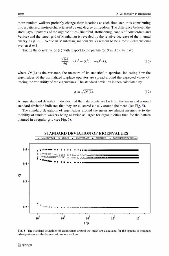
Taking the derivative of 〈λ〉 with respect to the parameter β in (15), we have

d〈λ〉dβ

= 〈λ〉2 − 〈λ2〉 = −D2(λ), (16)

where D2(λ) is the variance, the measure of its statistical dispersion, indicating how theeigenvalues of the normalized Laplace operator are spread around the expected value 〈λ〉tracing the variability of the eigenvalues. The standard deviation is then calculated by

σ =√

D2(λ). (17)

A large standard deviation indicates that the data points are far from the mean and a smallstandard deviation indicates that they are clustered closely around the mean (see Fig. 5).

The standard deviations of eigenvalues around the mean are almost insensitive to themobility of random walkers being as twice as larger for organic cities than for the patternplanned in a regular grid (see Fig. 5).

Fig. 5 The standard deviations of eigenvalues around the mean are calculated for the spectra of compacturban patterns via the laziness of random walkers


Fig. 6 The entropy of lazy random walks calculated for the spectra of compact urban patterns via the lazinessof random walkers

5.2 Entropy of Urban Space

In thermodynamics, entropy accounts for the effects of irreversibility describing the num-ber of possible observables in the system. For random walks defined on finite undirectedgraphs, its value,

S = −N∑

k=1

Prk ln Prk, (18)

quantifies the probable number of density distributions of random walks which can be ob-served in the system before the stationary distribution π is achieved.

In Fig. 6, we have displayed the entropy curves versus temperature in the studied cities.

6 Directed and Interacting Transport Networks

Many transport networks are naturally abstracted as directed graphs.Traffic within large cities is formally organized with marked driving directions creating

one-way streets. It is well known empirically that the use of one-way streets would greatlyimprove traffic flow since the speed of traffic is increased and intersections are simplified.

Up to our knowledge, there is just a few works in so far devoted to the analysis of complexdirected networks. Furthermore, the global transport network in the city usually consists ofmany different transportation modes which can be used alternatively by passengers whiletravelling (say, by trams, buses, subway, private vehicles, and by foot) at certain transportstations or elsewhere. Interactions between the individual transportation modes by means ofpassengers are responsible for the multiple complex phenomena we may daily observe onstreets and while using the public transportation.


The spectral approach for directed graphs has not been as well developed as for undi-rected graph. Indeed, it is rather difficult if ever possible to define a unique self-adjointoperator on directed graphs.

In general, any node i ∈ V in a directed graph �G can have different number of in-neighbors and out-neighbors,

kin(i) �= kout(i). (19)

In particular, a node i is a source if kin(i) = 0, kout(i) �= 0, and is a sink if kout(i) = 0,kin(i) �= 0. If the graph has neither sources nor sinks, it is called strongly connected.

A recent investigation by [31] shows that directed networks often have very few shortloops as compared to finite random graph models. In directed networks, the correlationbetween number of incoming and outgoing edges modulates the expected number of shortloops—if the values kin(i) and kout(i) are not correlated, then the number of short loops isstrongly reduced as compared to the case when both degrees are positively correlated.

6.1 Random Walks on Directed Graphs

Finite random walks are defined on a strongly connected directed graph �G(V, �E) as finitevertex sequences w = {v0, . . . , vn} (time forward) and w′ = {v−n, . . . , v0} (time backward)such that each pair (vi−1, vi) of vertices adjacent either in w or in w′ constitutes a directededge vi−1 → vi in �G.

A time forward random walk is defined by the transition probability matrix [32] Pij foreach pair of nodes i, j ∈ �G by

Pij ={

1/kout(i), i → j,

0, otherwise,(20)

which satisfies the probability conservation property:

∑

j,i→j

Pij = 1. (21)

The definition (20) can be naturally extended for weighted graphs [32] with wij > 0,

Pij = wij∑

s∈V wis

. (22)

Matrices (20) and (22) are real, but not symmetric and therefore have complex conjugatedpairs of eigenvalues. For each pair of nodes i, j ∈ �G, the forward transition probability isgiven by p

(t)ij = (Pt )ij that is equal zero, if �G does not contain a directed path from i to j .

Backwards time random walks are defined on the strongly connected directed graph �Gby the stochastic transition matrix

P �ij =

{1/kin(i), j → i,

0, otherwise,(23)

satisfying another probability conservation property

∑

i,i→j

P �ij = 1. (24)


It describes random walks unfolding backwards in time: should a random walker arrives att = 0 at a node v0, then

p(−t)ij = ((P�)t )ij (25)

defines the probability that t steps before it had originated from a node j . The matrix element(25) is zero, provided there is no directed path from j to i in �G.

If �G is strongly connected and aperiodic, the random walk converges [32–35] to theunique stationary distribution π given by the Perron vector, πP = π . If the graph �G isperiodic, then the transition probability matrix P can have more than one eigenvalue withabsolute value 1 [20]. The components of Perron’s vector π can be normalized in such away that

∑i πi = 1. The Perron vector for random walks defined on a strongly connected

directed graph can have coordinates with exponentially small values [32].Given an aperiodic strongly connected graph �G, a self-adjoint Laplace operator L = L�

can be defined [32] by setting

Lij = δij − 1

2

(π1/2Pπ−1/2 + π−1/2P�π1/2

)ij, (26)

where π is a diagonal matrix with entries πi . The matrix (26) is symmetric and has realnon-negative eigenvalues 0 = λ1 < λ2 ≤ · · · ≤ λN and real eigenvectors.

It can be easily proven [36] that the Laplace operator (26) defined on the aperiodicstrongly connected graph �G is equivalent to the Laplace operator defined on a symmetricundirected weighted graph Gw on the same vertex set with weights defined by

wij = πiPij + πjPji . (27)

6.2 Bi-orthogonal Decomposition of Random Walks Defined on Strongly ConnectedDirected Graphs

In order to define the self-adjoint Laplace operator (26) on aperiodic strongly connecteddirected graphs, we have to know the stationary distributions π of random walkers. Even ifπ exists for a given directed graph �G, it can be evaluated usually only numerically in polyno-mial time [33]. Stationary distributions on aperiodic general directed graphs are not so easyto describe since they are typically non-local in sense that each coordinate πi would dependupon the entire subgraph (the number of spanning arborescences of �G rooted at i [33]), butnot on the local connectivity property of a node itself like it was the case for undirectedgraphs. Furthermore, if the greatest common divisor of its cycle lengths in �G exceeds 1,then the transition probability matrices (20) and (23) can have several eigenvectors belong-ing to the largest eigenvalue 1, so that the definition (26) of Laplace operator seems to bequestionable.

Given a strongly connected directed graph �G specified by the adjacency matrixA �G �= A�

�G, we consider two random walks operators. A first transition operator representedby the matrix

P = D−1outA �G, (28)

in which Dout is a diagonal matrix with entries kout(i), describes the time forward randomwalks of the nearest neighbor type defined on �G. Given a time forward vertex sequence w

rooted at i ∈ �G, the matrix element Pij gives the probability that j ∈ �G is the vertex next to


i in w. A second transition operator, P�, is dynamically conjugated to (28),

P� = D−1in A�

�G= D−1

in P�Dout,(29)

where Din is a diagonal matrix with entries kin(i). The transition operator (29) describesrandom walks over time backward vertex sequences w′.

It is worth to mention that on undirected graphs P� ≡ P, since kin(i) = kout(i) for ∀i ∈ �Gand AG = A�

G. While on directed graphs, P� is related to P by the transformation

P = D−1out

(P�

)�Din, (30)

so that these operators are not symmetric, in general P� �= P�.We can define two different measures

μ+ =∑

j

degout(j)δ(j), μ− =∑

j

degin(j)δ(j) (31)

associated with the out- and in-degrees of nodes of the directed graph. In accordance to (31),we define two Hilbert spaces H+ and H− corresponding to the spaces of square summablefunctions, 2(μ+) and 2(μ−), by setting the norms as

‖x‖H± = √〈x, x〉H± ,

where 〈·, ·〉H± denotes the inner products with respect to measures (31). Then a functionf (j) defined on the set of graph vertices is fH−(j) ∈ H− if transformed by

fH−(j) → J−f (j) ≡ μ−−1/2j f (j) (32)

and fH+(j) ∈ H+ while being transformed accordingly to

fH+(j) → J+f (j) ≡ μ+−1/2j f (j). (33)

The obvious advantage of the measures (31) against the natural counting measure μ0 =∑i∈V δi is that the matrices of the transition operators P and P � are transformed under the

change of measures as

Pμ = J−1+ PJ−, P �

μ = J−1− P �J+, (34)

and become adjoint,

(Pμ

)ij

= A �Gij√kout(i)

√kin(j)

,

(P �

μ

)ij

≡ (P �

μ

)ij

= A��Gij√

kin(i)√

kout(j).

(35)

It is also important to note that

Pμ : H− → H+ and P �μ : H+ → H−.


We obtain the singular value dyadic expansion (biorthogonal decomposition introduced in[37, 38]) for the transition operator:

Pμ =N∑

s=1

�sϕsiψsi ≡N∑

s=1

�s |ϕs〉〈ψs |, (36)

where 0 ≤ �1 ≤ · · · ≤ �N and the functions ϕk ∈ H+ and ψk ∈ H− are related by theKarhunen-Loève dispersion [39, 40],

Pμϕs = �sψs (37)

satisfying the orthogonality condition:

〈ϕs,ϕs′ 〉H+ = 〈ψs′ ,ψs〉H− = δs′s . (38)

Since the operators Pμ and P �μ act between different Hilbert spaces, the solution of one

eigenvalue problem is not enough in order to determine their eigenvectors ϕs and ψs [41].Instead, two equations have to be solved,

{Pμϕ = �ψ,

P�μψ = �ϕ,

(39)

or, equivalently,(

0 Pμ

P�μ 0

)(ϕ

ψ

)

= �

(ϕ

ψ

)

. (40)

The latter equation allows for a graph-theoretical interpretation. The block anti-diagonaloperator matrix in the left hand side of (40) describes random walks defined on a bipartitegraph. Bipartite graphs contain two disjoint sets of vertices such that no edge has both end-points in the same set. However, in (40), both sets are formed by one and the same nodesof the original graph �G on which two different random walk processes specified by theoperators Pμ and P �

μ are defined.It is obvious that any solution of (40) is also a solution of the system

Uϕ = �2ϕ, V ψ = �2ψ, (41)

in which U ≡ P�μPμ and V ≡ PμP�

μ , although the converse is not necessarily true. Theself-adjoint nonnegative operators U : H− → H− and V : H+ → H+ share one and thesame set of eigenvalues �2 ∈ [0,1], and the orthonormal functions {ϕk} and {ψk} constitutethe orthonormal basis for the Hilbert spaces H+ and H− respectively. The Hilbert-Schmidtnorm of both operators,

tr(P �

μ Pμ

) = tr(PμP �

μ

) =N∑

s=1

�2s (42)

is a global characteristic of the directed graph.Provided the random walks are defined on a strongly connected directed graph �G, let us

consider the functions ρ(t)(s) ∈ [0,1]×Z+ representing the probability for finding a randomwalker at the node s, at time t . A random walker located at the source node s can reach


the node s ′ through either nodes. Being transformed in accordance to (32) and (33), thesefunction takes the following forms: (ρ(t)

s )H− = μ−1/2− ρ(t)(s) and (ρ(t)

s )H+ = μ−1/2+ ρ(t)(s).

Then, the self-adjoint operators U : H− → H− and V : H+ → H+ with the matrix elements

Uss′ = 1√kout(s)kin(s ′)

∑

i∈ �G

A��GisA �Gis′

√kout(i)kin(i)

,

Vs′s = 1√kout(s ′)kin(s)

∑

i∈ �G

A �Gs′iA��Gsi√

kout(i)kin(i)

(43)

define the dynamical system

⎧⎪⎪⎪⎨

⎪⎪⎪⎩

∑

s∈ �G

(ρ(t)

s

)H− Uss′ =

(ρ

(t+2)

s′)

H−,

∑

s′∈ �G

(ρ

(t)

s′)

H+Vs′s = (

ρ(t+2)s

)H+ .

(44)

The spectral properties of the self-adjoint operators U and V driving two Markov processeson strongly connected directed graphs and sharing the same non-negative eigenvalues �2

s ∈[0,1] can be analyzed separately by the method of characteristic functions as we did in theSect. 5.

The self-adjoint operators U and V describe correlations between flows of random walk-ers entering and leaving nodes in a directed graph—the strongest correlations are labelledby the largest eigenvalues �2

k , k = 1, . . . ,N .

6.3 Self-adjoint Operators for Interacting Networks

The bi-orthogonal decomposition can also be implemented in order to determine coherentsegments of two or more interacting networks defined on one and the same set of nodes V ,|V | = N .

Given two different strongly connected weighted directed graphs �G1 and �G2 specifiedon the same set of N vertices by the non-symmetric adjacency matrices A(1), A(2), whichentries are the edge weights, w

(1,2)ij ≥ 0, then the four transition operators of random walks

can be defined on both networks as

P(α) =(

D(α)out

)−1A(α),

(P(α)

)� =(

D(α)

in

)−1A(α), α = 1,2, (45)

where Dout/in are the diagonal matrices with the following entries:

k(α)out (j) =

∑

i,j→i

w(α)ji , k

(α)

in (j) =∑

i,i→j

w(α)ij , α = 1,2. (46)

We can define 4 different measures,

μ(1)− =

∑

j

k(1)out(j)δ(j), μ

(1)+ =

∑

j

k(1)

in (j)δ(j),

μ(2)− =

∑

j

k(2)out(j)δ(j), μ

(2)+ =

∑

j

k(2)

in (j)δ(j),(47)


and four Hilbert spaces H(α)± associated with the spaces of square summable functions,

2(μ(α)± ), α = 1,2.

Then the transitions operators P (α)μ : H(α)

− → H(α)− and (P (α)

μ )� : H(α)+ → H(α)

+ adjoint with

respect to the measures μ(α)± are defined by the following matrices:

(P (α)

μ

)ij

= A(α)

�G ij√

k(α)out (i)

√k

(α)

in (j)

,

(P (α)

μ

)�

ij= A(α)�

�Gij√

k(α)

in (i)

√

k(α)out (j)

.

(48)

The spectral analysis of the above operators requires that four equations be solved:

{P(α)

μ ϕ(α) = �(α)ψ(α),

P(α)μ

�ψ(α) = �(α)ϕ(α),(49)

where α = 1,2 as usual.Any solution {ϕ(α),ψ(α)} of the system (49), up to the possible partial isometries,

G(α)ϕ(α) = ψ(α), (50)

also satisfies the system

P(2)μ

�P(1)μ P(1)

μ�P(2)

μ ψ(2) = (�(1)�(2)

)2ψ(2),

P(1)μ

�P(2)μ P(2)

μ�P(1)

μ ψ(1) = (�(1)�(2)

)2ψ(1),

P(1)μ P(1)

μ�P(2)

μ P(2)μ

�ϕ(1) = (�(1)�(2)

)2ϕ(1),

P(2)μ P(2)

μ�P(1)

μ P(1)μ

�ϕ(2) = (�(1)�(2)

)2ϕ(2),

(51)

in which (�(1)�(2))2 ∈ [0,1]. Operators in the l.h.s of the system (51) describe correlationsbetween flows of random walkers which go through vertices following the links of eithernetworks. Their spectrum can also be investigated by the methods discussed in the previoussubsection.

It is convenient to represent the self-adjoint operators from the l.h.s. of (51) by the closeddirected paths shown in the diagram in Fig. 7. Being in the self-adjoint products of transition

Fig. 7 Self-adjoint operators fortwo interacting networks sharingthe same set of nodes


operators, P (α)μ corresponds to the flows of random walkers which depart from either net-

works, and P (α)μ

� is for those which arrive at the network α. From Fig. 7 , it is clear that theself-adjoint operators in (51) represent all possible closed trajectories visiting both networksN1 and N2.

In general, given a complex system consisting of n > 1 interacting networks operatingon the same set of nodes, we can define 2n self-adjoint operators related to the differentmodes of random walks. Then the set of network nodes can be separated into a number ofessentially correlated segments with respect to each of self-adjoint operators.

7 Conclusion

In the present paper, we have developed a self-consistent approach to complex transportnetworks based on the use of Markov chains defined on their graph representations.

Flows of pedestrians, private vehicles, and public transportation through the city are de-pendent on one another and have to be organized in a network setting.

We have shown that any strongly connected directed graph �G can be considered as abipartite graph with respect to the in- and out-connectivity of nodes. The bi-orthogonal de-composition of random walks is then used in order to define the self-adjoint operators ondirected graphs describing correlations between flows of random walkers which arrive atand leave the nodes. These self-adjoint operators share the non-negative real spectrum ofeigenvalues, but different orthonormal sets of eigenvectors. The global characteristics ofthe directed graph and its components can be obtained from the spectral properties of theself-adjoint operators.

The approach we have discussed in the present paper helps to define an equilibrium statefor complex transport networks and investigate its properties.

Acknowledgement The work has been supported by the Volkswagen Foundation (Germany) in the frame-work of the project: “Network formation rules, random set graphs and generalized epidemic processes” (Con-tract no Az.: I/82 418).

References

1. Braess, D.: Über ein Paradoxon aus der Verkehrsplannung. Unternehmensforschung 12, 258–268 (1968)2. Kolata, G.: What if they closed the 42nd Street and nobody noticed? The New York Times, Dec. 25

(1990)3. Alexanderson, G.L.: Bull. Am. Math. Soc. 43, 567–573 (2006)4. Hillier, B., Hanson, J.: The Social Logic of Space. Cambridge University Press, Cambridge (1984). ISBN

0-521-36784-05. Hillier, B.: Space is the Machine: A Configurational Theory of Architecture. Cambridge University Press,

Cambridge (1999). ISBN 0-521-64528-X6. Rosvall, M., Trusina, A., Minnhagen, P., Sneppen, K.: Phys. Rev. Lett. 94, 028701 (2005)7. Cardillo, A., Scellato, S., Latora, V., Porta, S.: Phys. Rev. E 73, 066107 (2006)8. Porta, S., Crucitti, P., Latora, V.: Physica A 369, 853 (2006)9. Scellato, S., Gardillo, A., Latora, V., Porta, S.: Eur. Phys. J. B 50, 221 (2006)

10. Crucitti, P., Latora, V., Porta, S.: Chaos 16, 015113 (2006)11. Volchenkov, D., Blanchard, Ph.: Phys. Rev. E 75(2) (2007)12. Volchenkov, D., Blanchard, Ph.: Physica A 387(10), 2353–2364 (2008). doi:10.1016/j.physa.2007.

11.04913. Gross, D., Harris, C.M.: Fundamentals of Queueing Theory. Wiley, New York (1998)14. Backus, B.T., Oruç, I.: J. Vis. 5(11), 1055–1069 (2005)15. Biggs, N.: Permutation Groups and Combinatorial Structures. Cambridge University Press, Cambridge

(1979)

http://dx.doi.org/10.1016/j.physa.2007.11.049

http://dx.doi.org/10.1016/j.physa.2007.11.049


16. Blanchard, Ph., Volchenkov, D.: Intelligibility and first passage times in complex urban networks. Proc.R. Soc. A 464, 2153–2167 (2008). doi:10.1098/rspa.2007.0329

17. Lagrange, J.-L.: Uvres, vol. 1, pp. 72–79. Gauthier-Villars, Paris (1867) (in French)18. Lovász, L.: Combinatorics, Paul Erdös is Eighty. Bolyai Society Mathematical Studies, vol. 2, pp. 1–46.

Bolyai Mathematical Society, Keszthely (1993)19. Aldous, D.J., Fill, J.A.: Reversible Markov chains and random walks on graphs (in preparation). See

http://www.stat.berkeley.edu/waldous/RWG/book.html20. Chung, F.: Lecture Notes on Spectral Graph Theory. AMS, Providence (1997)21. Farkas, I.J., Derényi, I., Barabási, A.-L., Vicsek, T.: Phys. Rev. E 64, 026704 (2001)22. Farkas, I., Derényi, I., Jeong, H., Neda, Z., Oltvai, Z.N., Ravasz, E., Schubert, A., Barabási, A.-L.,

Vicsek, T.: Physic A 314, 25 (2002)23. Abramowitz, M., Stegun, I.A. (eds.): Handbook of Mathematical Functions with Formulas, Graphs, and

Mathematical Tables. Dover, New York (1972)24. Sinai, Ya.G., Soshnikov, A.B.: Funct. Anal. Appl. 32(2), 114–131 (1998)25. Arnold, L.: Z. Wahrscheinlichkeitstheorie und Verw. Gebiete 19, 191–198 (1971)26. Alon, N., Krivelevich, M., Vu, V.H.: Isr. J. Math. 131, 259–267 (2002)27. Dorogovtsev, S.N., Goltsev, A.V., Mendes, J.F.F., Samukhin, A.N.: Phys. Rev. E 68, 046109 (2003)28. Eriksen, K.A., Simonsen, I., Maslov, S., Sneppen, K.: Phys. Rev. Lett. 90(14), 148701 (2003)29. Chung, F., Lu, L., Vu, V.: Proc. Natl. Acad. Sci. USA 100(11), 6313–6318 (2003). Published online

doi:10.1073/pnas.093749010030. Bollobás, B., Riordan, O.: Mathematical results on scale-free random graphs. In: Handbook of Graphs

and Networks. Wiley, New York (2002)31. Bianconi, G., Gulbahce, N., Motter, A.E.: Local structure of directed networks, 27 July 2007. E-print

arXiv:0707.4084 [cond-mat.dis-nn]32. Chung, F.: Ann. Comb. 9, 1–19 (2005)33. Lovász, L., Winkler, P.: Mixing of random walks and other diffusions on a graph. In: Surveys in Com-

binatorics, Stirling. London Math. Soc. Lecture Note Ser., vol. 218, 119–154. Cambridge Univ. Press,Cambridge (1995)

34. Bjöner, A., Lovász, L., Shor, P.: Eur. J. Comb. 12, 283–291 (1991)35. Bjöner, A., Lovász, L.: J. Algebr. Comb. 1, 305–328 (1992)36. Butler, S.: Electron. J. Linear Algebra 16, 90 (2007)37. Aubry, N., Guyonnet, R., Lima, R.: J. Stat. Phys. 64, 683–739 (1991)38. Aubry, N.: Theor. Comput. Fluid Dyn. 2, 339–352 (1991)39. Karhunen, K.: Ann. Acad. Sci. Fenn. A 1 (1944)40. Loève, M.: Probability Theory. van Nostrand, New York (1955)41. Aubry, N., Lima, L.: Spatio-temporal symmetries. Preprint CPT-93/P. 2923, Centre de Physique Theo-

rique, Luminy, Marseille, France (1993)

http://dx.doi.org/10.1098/rspa.2007.0329

http://www.stat.berkeley.edu/waldous/RWG/book.html

http://dx.doi.org/10.1073/pnas.0937490100

http://arxiv.org/abs/arXiv:0707.4084

Markov Chain Methods for Analyzing Urban...

Documents

Transcript of Markov Chain Methods for Analyzing Urban...