Markov Chain Monte Carlo Methods

Jesus Fernandez-VillaverdeUniversity of Pennsylvania

1

“Bayesianism has obviously come a long way. It used to be that could tell

a Bayesian by his tendency to hold meetings in isolated parts of Spain

and his obsession with coherence, self-interrogations, and other

manifestations of paranoia. Things have changed...”

Peter Clifford, 1993

2

Our Goal

• We have a distribution:X ∼ f(X)

such that f > 0 andRf(x)dx <∞.

• How do we draw from it?

• We could use Important Sampling...

• ...but we need to find a good source density.3

Five Problems

1. A Multinomial Probit Model.

2. A Markov-Switching Model

3. A Stochastic Volatility Model.

4. A Drifting-Parameters VAR Model.

5. A DSGE Model.

4

A Multinomial Probit Model (MNP)

• MNP goes back to Thurstone (1927) and Bock and Jones (1968).

• An individual i gets utility Uij from choice j, j ∈ {0, 1, ..., J} .

• Utility is given by Uij = xijβ + εij where εij are multivariate normal.

• Examples: car demand, educational choice, voting,...

5

Problem with MNP

• Under utility maximization, the individual will choose j with probabil-ity:

P³Uij > Uik, for all k 6= j

´=

Z ∞−∞

Z Uij−∞

...Z Uij−∞

f³Ui1,..., UiJ

´dUi1,...dUiJ

where f is the J−dimensional normal density.

• Two problems:

1. We need to evaluate a multidimensional normal integral.

2. Conditional on an evaluation of the integral, we need to draw fromthe posterior or maximize the likelihood.

6

First Problem: Multidimensional Integral

• Lerman and Manski (1981): Acceptance Sampling.

• GHK (Geweke-Hajivassiliou-Keane) simulator.

Second Problem: Manipulating the Likelihood

• Do we have good importance sampling densities to do so?

• Relation with MSM (McFadden, 1989).

7

Markov-Switching Model

• Hamilton (1979), Kim and Nelson (1999).

• Regression:zt = ρstzt−1 + e

σstεt where εt ∼ N (0, 1)

where

ρst = ρ0St + ρ1 (1− St)σst = σ0St + σ1 (1− St)

and transition matrix for St = {0, 1}Ãθ 1− θ1− λ λ

!

8

Stochastic Volatility Model

• Changing volatility clustered over time: Kim, Shephard, and Chib(1997).

• We have an autoregressive process:zt = ρzt−1 + eσtεt where εt ∼ N (0, 1)

1. and

σt = (1− λ)σmean + λσt−1 + τηt where ηt ∼ N (0, 1)

• How do we write the likelihood? Comparison with GARCH(p,q) (En-gle, 1982, and Bollerslev, 1986).

9

Drifting-Parameters VAR

• We have a VAR of the form:Yt = BtYt−1 + εt where εt ∼ N (0,Σ)

• The parameters Bt drift over time:Bt = Bt−1 + ωt where ωt ∼ N (0, V )

• Cogley and Sargent (2001) and (2002): inflation dynamics in the U.S.

10

DGSE Models

• We have a likelihood f³Y T |θ

´that does not belong to any known

parametric family.

• In fact, usually we cannot even write it: only obtain a (possibly sto-chastic) evaluation.

• Example: basic RBC model.

11

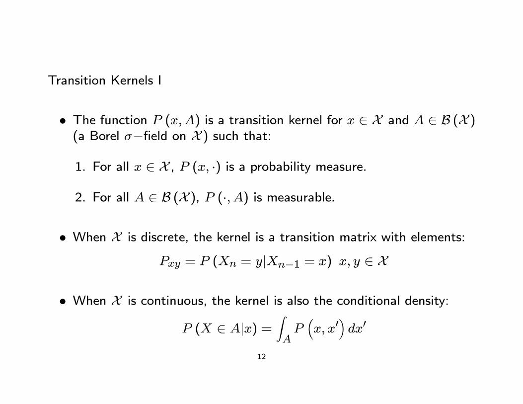
Transition Kernels I

• The function P (x,A) is a transition kernel for x ∈ X and A ∈ B (X )(a Borel σ−field on X ) such that:

1. For all x ∈ X , P (x, ·) is a probability measure.

2. For all A ∈ B (X ), P (·, A) is measurable.

• When X is discrete, the kernel is a transition matrix with elements:

Pxy = P (Xn = y|Xn−1 = x) x, y ∈ X

• When X is continuous, the kernel is also the conditional density:

P (X ∈ A|x) =ZAP³x, x0

´dx0

12

Transition Kernels II

• Clearly:P (x,X ) = 1

• Also, we allow:P (x,X ) 6= 0

• Examples in economics: capital accumulation, job search, prices infinancial market,...

13

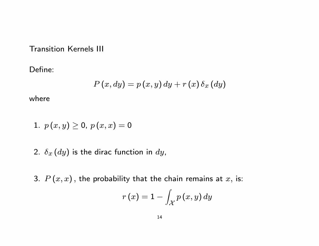
Transition Kernels III

Define:

P (x, dy) = p (x, y) dy + r (x) δx (dy)

where

1. p (x, y) ≥ 0, p (x, x) = 0

2. δx (dy) is the dirac function in dy,

3. P (x, x) , the probability that the chain remains at x, is:

r (x) = 1−ZXp (x, y) dy

14

Markov Chain

• Given a transition kernel P , a sequence X0,X1, ...,Xn, ... of randomvariables is a Markov Chain, denoted by (Xn), if for any t

P¡Xk+1 ∈ A|x0, ..., xk

¢= P

¡Xk+1 ∈ A|xk

¢=ZAP (xk, dx)

• We will only deal with time homogeneous chains, i.e., the distrib-ution of

³Xt1, ...,Xtk

´given x0 is the same as the distribution of³

Xt1−t0, ...,Xtk−t0´given x0 for every k and every (k + 1)−uplet

t0 ≤ ... ≤ tk.

15

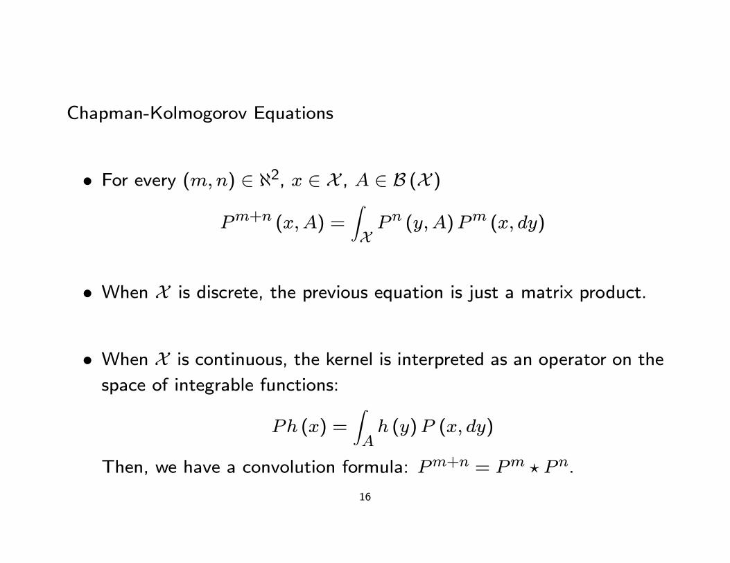
Chapman-Kolmogorov Equations

• For every (m,n) ∈ ℵ2, x ∈ X , A ∈ B (X )

Pm+n (x,A) =ZXPn (y,A)Pm (x, dy)

• When X is discrete, the previous equation is just a matrix product.

• When X is continuous, the kernel is interpreted as an operator on the

space of integrable functions:

Ph (x) =ZAh (y)P (x, dy)

Then, we have a convolution formula: Pm+n = Pm ? Pn.

16

Importance of Result

• More in general, we have an operator

Pπ (B) =ZAP (x,B)π (dx) , for all A ∈ B (X )

where π is a probability distribution.

• We can search for a fixed point:πs = Pπs

• We say that the distribution πs is invariant for the transition kernel

P (·, ·) .17

Relevant Questions

• Why do we care about a fixed point of the operator?

• Does it exist an invariant distribution?

• Do we converge to it?

• Meyn, S.P. and R.L. Tweedie (1993), Markov Chains and StochasticStability. Springer-Verlag.

18

Markov Chain Monte Carlo Methods

• A Markov Chain Monte Carlo (McMc) method for the simulation

of f (x) is any method producing an ergodic Markov Chain whose

invariant distribution is f (x).

• Looking for a Markovian Chain, such that if X1,X2, ...,Xt is a real-ization from it

Xt→ X ∼ f (x)as t goes to infinity.

19

Turning the Theory Around

• Note twist we are giving to theory.

• Computing Equilibrium models: we know transition Kernel (from pol-

icy functions of the agents) and we compute the invariant distribution.

• McMc: we know invariant distribution and we search for transition

kernel that induces that invariant distribution.

• How do we find the transition kernel?

20

A Trivial Example

• Imagine we want to draw from a binomial with parameter 0.5.

• The simplest way: draw a u ∼ U [0, 1]. If u ≤ 0.5, then x = 1,otherwise x = 0.

• The Markov Chain way:

1. Simulate from transition matrixÃ0.5 0.50.5 0.5

!with initial state 1.

2. Every time the state is 1, make xt = 1. Otherwise x = 0.

21

Roadmap

We search for a transition kernel that:

1. Induces an unique stationary distribution with density f (x).

2. Stays within stationary distribution.

3. Converges to the stationary distribution.

4. A Law of Large Number Applies.

5. A Central Limit Theorem Applies.

22

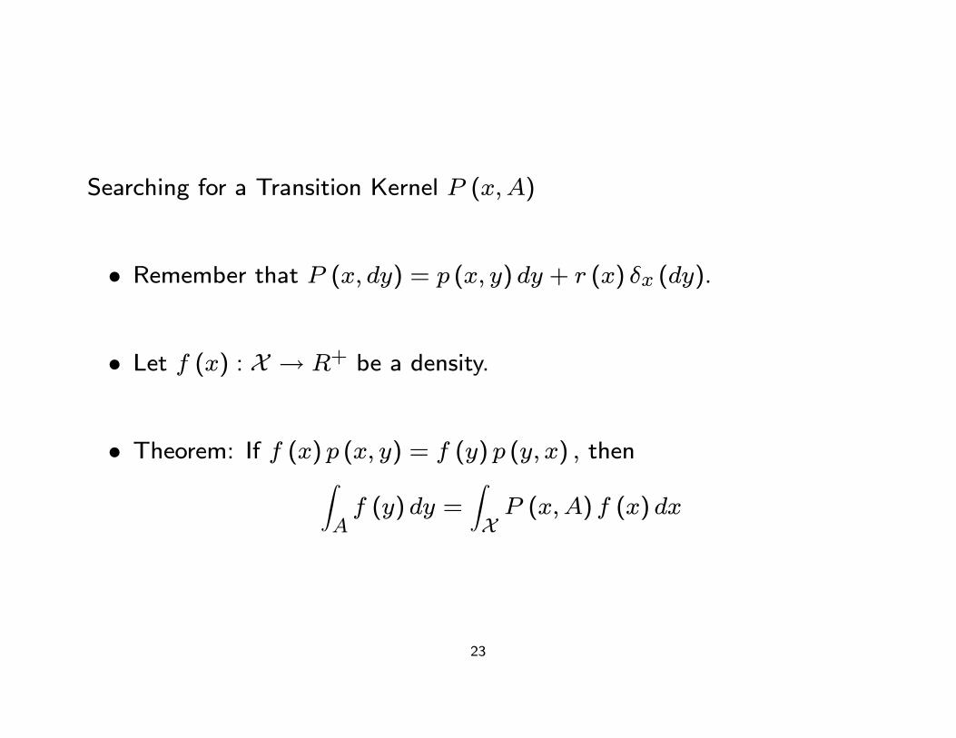
Searching for a Transition Kernel P (x,A)

• Remember that P (x, dy) = p (x, y) dy + r (x) δx (dy).

• Let f (x) : X → R+ be a density.

• Theorem: If f (x) p (x, y) = f (y) p (y, x) , thenZAf (y) dy =

ZXP (x,A) f (x) dx

23

Proof ZXP (x,A) f (x) dx

=ZX

·ZAp (x, y) dy

¸f (x) dx+

ZXr (x) δx (A) f (x) dx =

=ZA

·ZXp (x, y) f (x) dx

¸dy +

ZAr (x) f (x) dx =

=ZA

·ZXp (y, x) f (y) dx

¸dy +

ZAr (x) f (x) dx =

=ZA(1− r (y)) f (y) dy +

ZAr (x) f (x) dx =

=ZAf (y) dy

24

Remarks

• Note that RA f (y) dy = RX P (x,A) f (x) dx is an expression for the

invariant distribution. We will call that distribution πs.

• Explanation: if p (x, y) is time reversible, then f is the invariant dis-tribution of P (x, ·) .

• Time reversibility is the key element we will search for in our McMcalgorithms.

25

Convergence

• Note we have proved that the transition Kernel is a fixed point on thespace of densities.

• Can we prove convergence to that invariant distribution?

• If {Pn (x,A)}mn=0 where Pn (x,A) =RX P (y,A)Pn−1 (x, dy) and

P 0 (x,A) = P (x,A) , when do we have that:

Pm (x,A)→ πs (A)

for πs−almost all x ∈ X as m→∞ in the total variance distance?

26

Sufficient Conditions for Convergence

If P (x,A) is such that (1) holds, then the following two conditions about

P (x,A) are sufficient for Φm (x,A)→ πs (A) (Smith and Roberts, 1993):

• Irreducibility: if x ∈support(f)and A ∈ B (X ) , it should be possibleto get from x to A with positive probability in a finite number of steps.

• Aperiodicity: The Chain should not have periodic behavior.

Transient period (“burn-in”) in our simulations.

27

A Law of Large Numbers

If P (x,A) is irreducible with invariant distribution πs, then:

1. πs is unique.

2. For all πs−integrable real-valued functions:1

M

MXi=1

h (xi)→ZXh (x)πs (dx)

or bh→ Eh

almost surely.

How do we use this result?28

A Central Limit Theorem

• A Central Limit Theorem is useful to study sample-path averages.

• Two conditions on P (x,A):

1. Positive Harris-Recurrent.

2. Geometrically Ergodic.

29

Harris-Recurrence

• A set A is Harris-recurrent if Px (ηA =∞) = 1 for all x ∈ A.

• A Markov Chain is Harris-recurrent if it has an irreducible measure ψsuch that for every set A such that ψ (A) > 0, A is Harris-recurrent.

• Interpretation (Chan and Geyer, 1994): “Harris recurrence essentiallysays that there is no measure-theoretic pathology...The main point

about Harris recurrence is that asymptotics do not depend on the

starting distribution...”

30

Geometric Ergodicity

• An ergodic Markov chain with invariant distribution πs is geometricallyergodic if there exist a non-negative real-valued functions bounded in

expectation under πs and a positive constant r < 1 such that:°°°PM (x,A)− πs (A)°°° ≤ C (x) rn

for all x and all n and sets A.

• Geometric ergodicity ensures that the distance between the distribu-tion we have and the invariant distribution decreases sufficiently fast.

31

Chan and Geyer (1994)

If an ergodic Markov chain with invariant distribution πs is geometrically

ergodic, then for all L2 measurable functions h and any initial distribution

M0.5³bh−Eh´→ N

³0,σ2h

´in probability, where:

σ2h = var³h³P 0 (x,A)

´´+ 2

∞Xk=1

covnh³P 0 (x,A)

´h³P 0 (x,A)

´o

Note the covariance induced by the Markov Chain structure of our problem.

32

Building our McMc

Previous arguments show that we need to find a transition Kernel P (x,A)such that:

1. It is time reversible.

2. It is irreducible.

3. It is aperiodic.

4. (Bonus Points) It is Harris-recurrent and Geometrically Ergodic.

Note: 1)-4) are sufficient conditions!

33

McMc and Metropolis-Hastings

• The Metropolis-Hastings algorithm is the ONLY known method of

McMc.

• Gibbs-Sampler is a particular form of Metropolis-Hastings.

• Many researchers have proposed almost-but-not-quite-so McMc. Be-ware of them!.

• Where is the frontier? Perfect Sampling.

34

On the Use of McMc

• We motivated McMc by the need to draw from a posterior distributionof parameters.

• Up to a point the motivation is misleading.

• Why?

1. McMc helps to draw from a distribution. It does not need to be a

posterior. Think of the multivariate integral in the MNP model.

2. McMc explores a distribution. It can be used for classical estima-

tion.35

Difficult Problems for Classical Estimation

1. Censored Median Regression for Linear and Non-linear problems (Pow-

ell, 1994).

2. Nonlinear IV estimation (Berry, Levinsohn, and Pakes, 1995).

3. Instrumental Quantile Regression.

4. Continuous-updating GMM (Hansen, Heaton, and Yaron, 1996).

5. DSGE Models.36

McMc and Classical Estimation I

• Emphasized by Victor Chernozhukov and Han Hong (2003).

• Idea: Laplace-Type Estimators (LTE).

• Define similarly to Bayesian but use general statistical criterion func-tion instead of the likelihood.

• Function Ln (θ) such that:n−1Ln (θ)→M (θ)

37

McMc and Classical Estimation II

• Define the transformation:

pn (θ) =eLn(θ)π (θ)ReLn(θ)π (θ) dθ

that induces a proper distribution.

• Then, the quasi-posterior mean is:bθ = Z

θpn (θ) dθ

can be approximated by draws from a McMc:

bθ = 1

M

MXi=1

θi

38