Marcel Chamarelli Gutierrez Populism in General Equilibrium ......Marcel Chamarelli Gutierrez...
52
Transcript of Marcel Chamarelli Gutierrez Populism in General Equilibrium ......Marcel Chamarelli Gutierrez...

Marcel Chamarelli Gutierrez
Populism in General Equilibrium:
Indirect E�ects on Political Support
DISSERTAÇÃO DE MESTRADO
DEPARTAMENTO DE ECONOMIA
Programa de Pós�graduação em Economia
Rio de JaneiroApril 2016
DBD
PUC-Rio - Certificação Digital Nº 1412607/CA

Marcel Chamarelli Gutierrez
Populism in General Equilibrium:
Indirect E�ects on Political Support
Dissertação de Mestrado
Dissertation presented to the Programa de Pós�graduação emEconomia of the Departamento de Economia , PUC�Rio as apartial ful�llment of the requirements for the degree of Mestreem Economia.
Advisor : Prof. Eduardo ZilbermanCo�Orientador: Prof. Tiago Berriel
Rio de JaneiroApril 2016
DBD
PUC-Rio - Certificação Digital Nº 1412607/CA
Marcel Chamarelli Gutierrez
Populism in General Equilibrium:
Indirect E�ects on Political Support
Dissertation presented to the Programa de Pós�graduação emEconomia of the Departamento de Economia , PUC�Rio as apartial ful�llment of the requirements for the degree of Mestreem Economia.
Prof. Eduardo Zilberman
AdvisorDepartamento de Economia � PUC�Rio
Prof. Tiago Berriel
Co�AdvisorDepartamento de Economia � PUC�Rio
Prof. Gabriel Ulyssea
Departamento de Economia - PUC-Rio
Prof. Pedro Cavalcanti
Escola de Pós Graduação em Economia - FGV-RJ
Prof. Monica Herz
Coordinator of the Centro de Ciências Sociais � PUC�Rio
Rio de Janeiro, April 5th, 2016
DBD
PUC-Rio - Certificação Digital Nº 1412607/CA

All rights reserved
Marcel Chamarelli Gutierrez
The author graduated in Economics from UFRJ in 2014.
Bibliographic data
Gutierrez, Marcel Chamarelli
Populism in General Equilibrium: Indirect E�ects onPolitical Support / Marcel Chamarelli Gutierrez; advisor:Eduardo Zilberman; co�orientador: Tiago Berriel. � Rio deJaneiro : PUC�Rio, Departamento de Economia, 2016.(em Inglês)
v., 51 f: il. ; 29,7 cm
1. Dissertação (mestrado) - Pontifícia UniversidadeCatólica do Rio de Janeiro, Departamento de Economia.
Inclui referências bibliográ�cas.
1. Economia � Tese. 2. Populismo. 3. Equilibrio Geral.4. Economia politica. 5. Suporte político. 6. Agentesheterogêneoes.I. Zilberman, Eduardo. II. Berriel, Tiago. III. PontifíciaUniversidade Católica do Rio de Janeiro. Departamento deEconomia. IV. Título.(em Português)
CDD: 330
DBD
PUC-Rio - Certificação Digital Nº 1412607/CA

Acknowledgments
Special thanks to my advisors, Tiago Berriel and Eduardo Zilberman,
for all the pacience and enlightenment; also to my classmates Leandro, John,
Gustavo, Moisés and Pedro for all the co�eebreaks and ideas, and without
whom this work would not be possible; and for last, not least, my family and
Jéssica.
DBD
PUC-Rio - Certificação Digital Nº 1412607/CA

Abstract
Gutierrez, Marcel Chamarelli; Zilberman, Eduardo(advisor);Berriel, Tiago. Populism in General Equilibrium: Indirect
E�ects on Political Support. Rio de Janeiro, 2016. 51p.MSc. Dissertation � Departamento de Economia, PontifíciaUniversidade Católica do Rio de Janeiro.
We present a version of the standard general equilibrium model
with heterogenous agents and incomplete markets to address matters
of populism and political support of governments. The novelty is to
assume that governments may expropriate part of the resources in the
economy. We highlight a new mecanism in which a populist government can
obtain the approval necessary to maintain power. Transfers to poorest/less
productive households increases the equilibrium interest rates, by reducing
precautionary savings, bene�ting rich capital holders and creating a
coalition between them. Further, we calibrate the model to a standard U.S
economy and conduct some comparative statics in key parameters to address
the likelihood of such arrangement.
Keywords
Populism; General Equilibrium; Political economy; Political
support; Heterogenous agents;
DBD
PUC-Rio - Certificação Digital Nº 1412607/CA

Resumo
Gutierrez, Marcel Chamarelli; Zilberman, Eduardo(orientador);Berriel, Tiago. Populismo em Equilíbrio Geral: Efeitos
Indiretos sobre Apoio Político. Rio de Janeiro, 2016. 51p.Dissertação de Mestrado � Departamento de Economia, PontifíciaUniversidade Católica do Rio de Janeiro.
Apresentamos uma versão do modelo padrão de equilíbrio geral
com agentes heterogêneos e mercados incompletos para responder questões
acerca do populismo e suporte político. A inovação é assumir que o
governo pode expropriar parte dos recusos da economia. Destacamos um
novo mecanismo de suporte político, onde o governo populista obtém a
aprovação necessária para se manter no poder. Transferências para os mais
pobres/menos produtivos aumentam a taxa de juros de equilíbrio, ao reduzir
a poupança por motivo precaucional, bene�ciando detentores de capital
ricos e criando uma coalizão entre eles. Então, fazemos um exercício de
calibração para a economia americana e conduzimos exercícios de estática
comparativa em parâmetros chave para analisar a verossimilhança do
arranjo.
Palavras�chave
Populismo; Equilibrio Geral; Economia politica; Suporte político;
Agentes heterogêneoes;
DBD
PUC-Rio - Certificação Digital Nº 1412607/CA

Contents
1 Introduction 10
2 Literature Review 13
3 General Model 16
3.1 Environment Overview 163.2 Households and Firm 173.3 Government 193.4 Equilibrium 213.5 Discussion 22
4 Parametrization and Results 24
4.1 Functional Forms and Parameters 244.2 Results 26
5 American Process for Wages and Comparative Statics 31
5.1 U.S. Economy Calibration 315.2 Comparative Statics on Wages Process 345.3 More States 43
6 Final Remarks 46
Bibliography 47
A Appendix 50
DBD
PUC-Rio - Certificação Digital Nº 1412607/CA

List of Figures
4.1 Political Support for each eligibility criterium 274.2 Savings e�ects on Interests 294.3 Equilibrium e�ects on Wages 29
5.1 Political Mechanism in U.S. Economy Calibration 335.2 Savings e�ects on Interest on U.S. Economy Calibration 355.3 Equilibrium e�ects on Wages on U.S. Economy Calibration 355.4 Political Support as a function of τ for U.S. Economy 375.5 σ2
ε and Interest Rates in Equilibrium 385.6 σ2
ε and Wages in Equilibrium 385.7 ρ and Interest Rates in Equilibrium 425.8 ρ and Wages in Equilibrium 425.9 Political Support and Eligibility Criterium 44
DBD
PUC-Rio - Certificação Digital Nº 1412607/CA

List of Tables
4.1 Parametrization 254.2 States and Stationary Distribution 254.3 Political Support and Wealth 28
5.1 U.S. Economy Calibration 325.2 Political Support and Wealth in U.S. Calibration 345.3 Comparative Statics on σ2
ε 365.4 σ2
ε and Capital in Equilibrium 395.5 Comparative Statics on σ2
ε with Exogenous Labour 415.6 Comparative Statics on ρ with Exogenous Labour 435.7 Political Support with 15 states 45
DBD
PUC-Rio - Certificação Digital Nº 1412607/CA

1
Introduction
What are the incentives faced by governors and voters when they
must choose how much to tax and transfer? How much redistribution is
necessary to maintain power in unequal societies? These are questions broadly
explored in the political economy literature. Robinson e Acemoglu (2006)
develops numerous models to explain the rational economic foundations of
democratic and authoritarians governments. Also, Krussel e Rios-Rull (1999),
Krussel et al. (1997), Krussel e Rios-Rull (1994) and Corbae et al. (2009)
uses quantitative and theoretical macroeconomic models to answer similar
questions, as how di�erent institutional arrangements induces di�erent growth
paths and how much of the level of taxation and distribution observed in
countries can we explain as political outcomes in quantitative macroeconomic
models.
One of the questions we would like to address is: can we use these various
contributions to understand the dynamic of expropriation and corruption in
development countries? Speci�cally, in an emergent economy where commodity
exportation is a large fraction of the GNP, what portion (if any) of these
products income can a governor con�scate, to whatever end, and still maintain
power? If that government desires to expropriate this commodity to which
fraction of the population will he �nd optimum transferring to?
The main inspiration for this paper is the political science work of
Mazzuca (2013). The author analyses the "left turn" that has been the major
political trend in many Latin American countries since the beginning of the
century. As Mazzuca (2013) called, the "rentier populism" that emerged on
these countries were characterized by a coalition between the incumbent
government, that redistributes natural resources earnings (experiencing often a
boom in international prices) to informal workers, and the informal sectors that
bene�t from these policies and legitimizes them through plebiscitarianism. On
the other hand, the constant expropriation of privately owned �rms generates
a latent ine�ciency and a troubling foreign investment getaway.
Mazzuca (2013) highlights the fact that this coalition was only possible
due to the boom in commodities prices, launched mainly by the accelerated
growth of India and China, improving the terms of trade of these products
exporting countries. The idea is that this boom elevated the incentives to
expropriate and made it possible to do so despite the distortions derived by it.
In this paper we try to model this work. We use a heterogeneous agent
DBD
PUC-Rio - Certificação Digital Nº 1412607/CA

Chapter 1. Introduction 11
with incomplete markets model, that we believe replicates reasonably well an
emergent economy, with an exogenous income that we chose to interpret as
a commodity income that can be divided among workers or expropriated by
the local government to non-productive means. We believe this framework is
fairly general and contemplates not only the cases Mazzuca (2013) calls rentier
populists coalitions and "superpresidentialism" in Latin American countries,
but also others authoritarian dominions in agricultural countries, as in African
examples. By doing that, we add some new insights to his initial analysis.
Mainly, we found that sometimes a coalition between poor low productive
households and rich capital owners can be formed that sustain the populist
government in power. As we will see, populism will raise endogenously, as a
solution to the government problem of maximizing the amount expropriated.
Acemoglu et al. (2013) de�nes populism as politics to the left of the median
voter. In our case, populism will be transferring to the poorest (the least
productive ones, it will be clear later why) households even if they are no
majority in the population. By doing so, the government induces an equilibrium
in which high interest rates bene�t the rich capital owners, that, therefore,
supports the incumbent government.
High interest rates in development economies such as the ones illustraded
by Mazzuca (2013) is quite usual. But the level of nominal and real interests
in these countries with left governments are usually associated with the
desincentives to savings and investing caused by expropriation risk. In our
work we do not consider e�ects of taxing on private individual incentives
to save, since we only allow the government to tax the exogenous income.
Instead, interest rises in equilibrium due to the decrease in risk perception
(and consequent decrease in precautionary savings) by, mainly, low income
households. When the policy maker chooses to focus transfers on households
that are most vulnerable to adverse shocks, it decreases the overall level os
savings in the economy, consequently elevating capital returns. The trade o�
they face is analogous: by reducing capital in equilibrium, wages are also
reduced. Rich households are also the most productive ones in the economy,
so they must choose between more capital return or more labour return. As
one should suspect, only extremely wealthy families �nd this attractive, and
the equilibrium outcome most harm the middle class.
Therefore, precautionary savings play a major role in our model. A
similar result is found in Krussel et al. (2009), but the authors use a business
cycle model to estimate the welfare gains from reducing aggregate shocks.
When the government chooses to transfer only to the least productive, in a
model where productivity is idiosyncratic as ours, that means an insurance
DBD
PUC-Rio - Certificação Digital Nº 1412607/CA

Chapter 1. Introduction 12
in the worst state of nature. Households, therefore, responds by reducing
precautionary savings, a�ecting the equilibrium level of capital and, hence,
interests and wages. Capital is decreased, as are wages, and interest rate
increases. The reduction in wages implies a trade-o�, and that is why, for
high productive households, only the wealthiest of all will be bene�ted by the
populist government. To the best of our knowledge, our work is the �rst to
address this kind of coalition on a general equilibrium framework.
Since we know from Aiyagari (1994) that precautionary savings can be
of little relevance in a more realistic calibration, we proceed by adapting
our parameters in a more fashion way. We choose to follow the work of
Floden e Lindé (2001) because insurance also plays a major role on their
results, and so we calibrate the model in similar way to theirs. We �nd
that, indeed, this coalition between poor and wealthy households that allows
a majority political support to the government is less likely to occur in an
American economy calibrated model. Also we induct a series of comparative
statics in parameters that determine the amount of risk and persistence of the
shocks in the economy. We found that economies with higher risk are more
likely to experience such an arrangement, although this is somehow dubious.
Albeit being essential to our result, precautionary savings can also be its
downfall. If asset accumulation for insurance reasons is too high in a standard
economy so that the consequent capital reduction that arises by transferring
to households in the worst state is very sharp, the reduction on equilibrium
wages are so high that weakens the mechanism (the political support given by
rich capital owners), even though interests rises considerably.
The rest of the paper is as follows: on Section I we will brie�y discuss
some of the literature in political economy and macroeconomics that served as
inspiration and support to this work; Section II we present the general model
we used to present our main results; Section III we will discuss the results and
the parametrization used; in Section IV we present the results for the American
calibration and perform comparative statics; Section V we conclude.
DBD
PUC-Rio - Certificação Digital Nº 1412607/CA

2
Literature Review
The main idea of this paper is to analyze the contribution of
Mazzuca (2013) in a general equilibrium framework. We do so by extending
Berriel e Zilberman (2011) model of focused direct transfers to poor workers,
by delegating the choice of how much to redistribute (and to whom) to a
governor that has its own utility function, as in ).
Berriel e Zilberman (2011) investigate how targeted cash transfer
programs increase the welfare in a developing economy. The channel here is
insurance. They use a incomplete market framework similar to ours, in which
the workers face an idiosyncratic productivity shock that lead to uninsurable
realizations of the endowment. Their results suggests that re-distributive
programs can have positive e�ects on general welfare by providing safeguard
to low income households. These households, initially binded by the borrowing
constraint, deeply bene�t from this additional income, reducing precautionary
savings and increasing consumption. In fact, even workers that are not eligible
for the program would support it (they claim that 77, 3% of the population
in a model parameterized for Brazil are better o� with the program). This
happens due to the possibility of adverse realizations of the shock in the
future, that now are secured by the eligibility for the program.
Corbae et al. (2009) presents us an economy with idiosyncratic shocks to
labor e�cient and incomplete markets, inspired by Aiyagari (1994) framework,
and model the choices of taxes with a political economy equilibrium, which
the median voter is the pivotal. The question they look forward to answer is
whether the increase in wage inequality, observed in U.S. data between late
70's and early 90's, as the decrease of median to mean wages can explain why
we observed also an increase in transfers to poor workers in that period. The
idea is that median voters choices tended to more distortionary taxation and
transfers, given the elevation of risk (which they claim to be the causation of
increased wage inequality).
Another paper of major importance in the literature of
quantitative political economy and choices of size of government is
Krussel e Rios-Rull (1999). The authors use a neoclassical growth frame,
with complete markets and di�erent productivities among workers (but no
uncertainty) and develop a dynamic voting general equilibrium model. Perfect
foresight becomes crucial here, since voters must predict perfectly all outcomes
of di�erent policies to choose consistently with rational expectations. Their
DBD
PUC-Rio - Certificação Digital Nº 1412607/CA

Chapter 2. Literature Review 14
predictions performs reasonably well against data, and seem more realistic
(after calibration) than a static model.
The role of the government as a provider of insurance is well documented
in Floden (2001), Floden e Lindé (2001) and Dos Reis e Zilberman (2014). All
of this papers use a framework of incomplete market and heterogeneous agents
similar to ours in a lot of sense, and thy to address matters of insurance.
Floden (2001) analyses how variations in public debt and transfers a�ect
risk sharing, e�ciency and the distribution of resources in the economy,
�nding that the government can signi�cantly improve risk sharing if using
debt and redistribution correctly. Floden e Lindé (2001) estimates income
process, as AR(1), for Sweden and U.S., comparing the degrees of risk faced
by households in each country, and insurance provision. They found that,
while in Sweden insurance provision is too high, in U.S. it is too low.
Dos Reis e Zilberman (2014) extends the general framework to account for
public and private employment. In Brazil, for instance, public employment
follows very di�erent aspects than private one with respect to the grade of
risk of dismissal. They �nd that public employment is an important provider
of insurance, although it provides for middle class families (with middle and
high productivities) and not the ones that requires it the most (low productive
households that are credit constrained).
The role of political economy in the dynamics of our model is simple, but
requires literature fundamental. In our analysis we try to replicate a delegative
democracy (not a direct one), so we do not use the median voter framework as
usual in the literature. Instead we borrow some insights from the dictatorship
models of Robinson e Acemoglu (2006) and Acemoglu e Robinson (2001).
There, the level of taxes and transfers are made solely by the governor (a
dictator) who faces a revolution constraint, which means his optimization is
subject to a wish to stay in power (they assume, in general, that the dictator
is in favor of the elite, so he maximizes the richest part of the population
utility, and that means less taxes). They �nd that highly unequal societies are
more likely to persist in dictatorship than more egalitarian (although they �nd
that too much equal also increases the odds). That is intuitive, and is aligned
with the stylized facts that Barro (1999) �nds in his empirical study of the
determinants of democracy. That is also something we address by comparative
statics. We �nd that more inequality usually increases the likelihood of a
populist arrangement like the one we present.
An alternative work we used as background to ours is ). It is an extension
of Berriel e Zilberman (2011) analysis of Bolsa Familia in Brazil, but put in
the hands of a government the choice of taxes and transfers, as the eligibility
DBD
PUC-Rio - Certificação Digital Nº 1412607/CA

Chapter 2. Literature Review 15
criterion for the program. Our government will be similar to that one in
his control variables, but will di�er in the objective function. In the next
section we will present our model, and therefore explore more of the literature's
contribution to our subject.
DBD
PUC-Rio - Certificação Digital Nº 1412607/CA

3
General Model
3.1
Environment Overview
Time is in�nite and discrete in a closed economy. There is a continuum of
risk averse households that will di�er only in their idiosyncratic productivity
of labor, and a representative �rm that replicates a competitive market for a
unique consumption good, which is perfectly convertible to capital. There is
only idiosyncratic risk in this economy but no aggregate uncertainty. Agents
maximize lifetime utility discounted by (the same) parameter β. Markets are
incomplete and the only saving possibility for a household is to rent capital to
the �rm, receiving an interest rate of r.
As shown in Aiyagari (1994) this type of model demands a borrowing
constraint, whether it be a natural one (meaning that an agent would have to
almost certain give up all of his future income to repay a loan of the amount
of the constraint) or an ad hoc one. In this work we follow the literature
and add an ad hoc borrowing limit, so families can save but cannot borrow
any positive amount. This will cause individuals to worry about receiving an
adverse shock and becoming constrained, bringing precautionary savings to
the matter (see Aiyagari (1994) for a detailed exposition of the subject). In
other words, in an incomplete market model with idiosyncratic uncertainty, the
impossibility of full insurance can be partially o�set if households are allowed
to borrow when faced with bad realizations of the random productivity (or
endowment) and save when favored by luck. With borrowing limits, this is not
possible, exacerbating the loss in welfare derived from the lack of insurance.
This framework is very close to the original Aiyagari (1994) model and is a
simpli�ed version of Berriel e Zilberman (2011) developing economy.
The innovation we propose, relative to these examples, is the presence of
an exogenous parameter B, that we assume to be constant every period. This
"manna" will be distributed to the population in the form of direct transfers,
and any part not distributed is fully consumed by the government. We think
of this as a re-distributive state case in Besley e Persson (2011) analysis.
The authors claim that a re-distributive state emerges when cohesiveness
on internal investment decisions are low (another interpretation in that
heterogeneity is high) but political stability is high enough. This case is
characterized by redistribution and investment in �scal capacity of the state
DBD
PUC-Rio - Certificação Digital Nº 1412607/CA

Chapter 3. General Model 17
(the ability to tax). We believe this is well applied to the cases exposed
in Mazzuca (2013), since these populist governments share high levels of
redistribution and a large and powerful state apparatus.
One interpretation here is that B is an exportation income from some
national commodity, but this is essentialy arbitrary. The only prerequisite
is that this income can be taxed without any kind of distortion since it
does not depends on individuals decision making to exist. Also, government
consumption has no e�ect on any variable in the model. We will refer to this
tax, sometimes, as expropriation since this is the term used by Mazzuca (2013).
Transfers here are similarly to the ones in Berriel e Zilberman (2011),
and are targeted to some speci�c fraction of the population, that are eligible
to receive them. The government will decide the threshold for which families
below it will receive (equally divided) the amount not taxed. That threshold
will be some level of productivity, for simplicity. Productivity here is only
a proxy to labor income, since agents can choose to work more or less. To
allow eligibility on total income (including capital rents) is computationally
costly, since the stationary distribution of agents is endogenous (see the next
section and the computational appendix). Furthermore, allowing the choice of
eligibility to be taken with respect to labor income, besides the fact that it
does not simplify the problem of endogeneity, would allow cases in which a
very wealthy agent that decides not to work receives the transfers. Since this
would be even worse for our purpose of replicate transfers directed to social
strata, we prefer to maintain the productivity-based eligibility criterion.
In this kind of model, productivity is publicly known and there is
no information asymmetry, therefore, the policy maker can observe each
individual level of productivity in each period and decide which levels will
be eligible. He cannot, however, arbitrarily choose any level of productivity,
since he must choose a threshold level from which every level below it will also
be eligible.
3.2
Households and Firm
Households di�er only in their stochastic productivity θ ∈ Θ, where
Θ is a �nite and countable set, and evolves according to a Markov chain
represented by a transition matrix P . That matrix must have a stationary
distribution, and it will have since accounted for the su�cient conditions
present in Ljungqvist e Sargent (2012). Individuals discount future at a rate
β, and each period they choose how much to consume and how much to save
to next period. Each worker is provided with one unit of labor that can be
DBD
PUC-Rio - Certificação Digital Nº 1412607/CA

Chapter 3. General Model 18
continuously o�ered in the interval [0, 1], at a wage w. The household problem
conditional on a determined level of redistribution is (recursively):
V (a, θ; τ, T, θ) = max{a′,n}
[U(c, n) + βEV (a′, θ′; τ, T, θ)]
subject to
c+ a′ =(1 + r − δ)a+ θwn+ I[θ≤θ]T
c ≥ 0
a′ ≥ b
n ∈ [0, 1],
Where x′ means a variable in the next period, a is the amount of individual
capital, r is the risk free interest rate, T is the amount of transfers and I
is an indicator function that equals 1 if the household is eligible to receive
the transfers, and 0 otherwise, w is the competitive wage, b is the borrowing
constraint (b ≤ 0) n are units of labor, c is consumption and τ and θ is the
expropriation parameter and eligibility criterion, respectively, that will arise
from the government problem and indexes individual decisions. U is a strictly
concave utility function and θ ∼ P (θ′, θ).
This is a standard consumer problem when faced with idiosyncratic
productivity, inability to self ensure and borrowing constraint. The concavity
imposed on the utility function is a su�cient condition for the existence
and unity of the optimum. So far the only di�erence between this
problem and a general one is the presence transfers T , but that is
hardly new since taxation and distribution problems have been extensively
studied in the literature as in Berriel e Zilberman (2011), Corbae et al. (2009),
Krussel e Rios-Rull (1999) and others. The indicator function for eligibility
is also not a novelty since these papers often work with directed transfers
(specially Berriel e Zilberman (2011)).
The solution to the problem above are functions g(a, θ), of optimum
savings, and n(a, θ), of optimum labor o�er. The stationary distribution
associated with this solution is λ(a, θ). This distribution is a function of both
individual capital and productivity, since it represents the mass of workers
that, in steady state, possess wealth of a with productivity θ. The technology
of the �rm is standard, constant returns to scale, and every period it maximizes
pro�t as in perfect competition, so Fk(K,N) = r+δ and Fn(K,N) = w, where
K =∫g(a, θ)dλ(a, θ) is total capital of the economy, δ is the depreciation rate
and N =∫θn(a, θ)dλ(a, θ) is the aggregate e�ciency labor measure.
DBD
PUC-Rio - Certificação Digital Nº 1412607/CA

Chapter 3. General Model 19
3.3
Government
Government chooses the productivity threshold (θ) and the amount of B
expropriated or taxed (τ ∈ [0, 1]) as to maximizes it's own utility. The utility
of the government is:
Ug = h(τB)
if he is in power and
Ug = −∞
otherwise
Where h is any strictly increasing function of τB. That means basically that,
whatever that implicates, the government will prefer to maintain power instead
of loosing it. It is certainly an important assumption that we are making, and
we chose to do so in ordert to guarantee that there will be an equilibrium in
which this government (that always wishes to tax more) will maintain power
inde�nitely. That will allow us to focus only on steady state allocations, which
greatly simpli�es the analysis.
Now we have to de�ne what determines that the control of the state does
not changes hands. Our simple assumption will be that if at least some fraction
χ of the population is better o� than when compared to an outside option,
than the current government will hold o�ce.
A question bound to arise is what do households take into account when
they decide whether they are content with the current government actions or
not? Here we will present an important assumption, which is the fact that
households only compare steady state allocations. This is a simpli�cation with
computational purposes. From here on one should recall that every time we
refer to an equilibrium allocation, this will be a stationary equilibrium.
Assumption 1 Households only compare steady state allocations when decide
whether or not to overthrown the government.
In order to retain power, rulers must to some extent bene�t at least
a fraction of the population when compared to the outside option that
is overthrowing the incumbent. On their work, Robinson e Acemoglu (2006)
impose a cost of surging, so agents would balance the bene�ts of a democratic
government (in their case a media-voter-guided policy) against the costs of
the rebellion. In our model we assume that the outside option is simply
an egalitarian government, with zero expropriation (whether the incumbent
DBD
PUC-Rio - Certificação Digital Nº 1412607/CA

Chapter 3. General Model 20
is overthrown via elections or revolution, since our model does not require
explicitly that the government be a dictatorship).
Assumption 2 The outside option government is one that equally distributes
B to all households.
So the government chooses τ ∈ [0, 1] and θ ∈ Θ. Before we formalize the
problem, it is interesting to notice that the outside option government is fully
characterized by the pair of potential solutions to the standard government
problem: τ = 0 and θ = ∞ (it is simply not taxing B and choosing θ to be
the supreme of Θ). That, on the other hand, implies a level of transfers that
we will call T .
The governor problem is, therefore:
max{τ,θ}
h(τB)
subject to∫I[θ≤θ]Tdλ(a, θ) =(1− τ)B∫
I[V (a,θ;τ,T,θ)>V (a,θ;0,T ,∞)]dλ(a, θ) > χ,
where χ ∈ (0, 1)
h′ > 0
The �rst constraint is the budget balance constraint. The government can
not operate with de�cits or surpluses (nor it would be optimum to do so).
The second one is derived from the form of the utility presented before. The
ruler always �nd it would be optimum to retain power, so we include it as
a constraint in his problem. It simply states that the mass of households in
which the lifetime value functions associated with the chosen allocation have
higher value than the ones associated with the outside option, is greater than
χ.
Note that T is fully determined by τ and θ, for a given B. It becomes
clear now why the productivity-based eligibility criterion makes things a lot
simpler. Although we express T as an integer on λ(a, θ) it only depends
on the distribution of agents among θ, and not the pair (a, θ) (because the
mass of workers with each productivity in steady state will always be the
same). That distribution depends solely on the transition matrix P (θ′, θ) (see
Ljungqvist e Sargent (2012)). Therefore, the mass of agents that will receive
DBD
PUC-Rio - Certificação Digital Nº 1412607/CA

Chapter 3. General Model 21
transfers is entirely determined by θ, and it is not an endogenously varying
element. That greatly simplify the computation of the equilibrium.
3.4
Equilibrium
Summing up, the government chooses τ , the amount of B taxed (or
expropriated), and θ, the eligibility threshold. Households optimum policies are
indexed by those choices and we will state them as g(a, θ; τ, θ) and n(a, θ; τ, θ).
Hence, the competitive equilibrium that will unfold is also indexed by the pair
suggested by the ruler. We de�ne the steady state competitive equilibrium as
follows:
De�nição 3.1 A Recursive Competitive Stationary Equilibrium for given
{B, δ, b, τ , θ} is a value function V (a, θ; τ , θ), policy functions g(a, θ; τ, θ) and
n(a, θ; τ, θ), a measure λ(a, θ; τ, θ) and prices {r(τ , θ), w(τ , θ)}, so that:
1. g(a, θ; τ, θ) and n(a, θ; τ, θ) solve the households problem for given
{r(τ , θ), w(τ , θ)};
2. The �rm maximizes it's pro�ts for given {r(τ , θ), w(τ , θ)}:
� Fk(K,N) = r + δ;
� Fn(K,N) = w;
3. Markets Clear:
�∫θn(a, θ)dλ(a, θ) = N ;
�∫g(a, θ)dλ(a, θ) = K;
4. Government budget balances: T = (1−τ)B∫I[θ≤θ]dλ(a,θ)
;
5. λ(a, θ; τ, θ) is an invariant probability measure.
The policy maker, thus, provided as he is with perfect information and
foresight, will choose a competitive equilibrium that maximizes his own utility,
similar to a Ramsey problem. The government will choose the competitive
equilibrium associated with the maximum τ possible so that he keeps a mass
of χ workers better o� than the egalitarian equilibrium. Since we are focusing
on steady state allocations, the solution τ will be constant. For the sake of
completeness and since we will use this de�nition further ahead, we de�ne our
political equilibrium.
De�nição 3.2 A Political Economic Stationary Equilibrium is an allocation
{τ∗, θ∗} that solves the government problem.
DBD
PUC-Rio - Certificação Digital Nº 1412607/CA

Chapter 3. General Model 22
Hence, we call a political economic equilibrium a pair {τ∗, θ∗} in which τ∗is the greater possible value between 0 and 1 so that the recursive competitive
stationary equilibrium indexed by it keeps χ households happier than the
outside option equilibrium. It is clear that, since we allow the choice of τ
to be continuous (at least theoretically), the policy maker will choose it in a
way that the mass of happy workers will be exactly χ.
3.5
Discussion
Before we move on we will comment some hypothesis we made. First, it
clear that our extension to include the commodity B is intentionally simple.
This commodity has no direct e�ect on output (but there will be indirect
e�ects, since it can be redistributed) and we do not formally model and
exportation sector or an international market (in fact, our economy is closed).
We know from Aguiar e Amador (2011) and Aguiar et al. (2009) and a much
extensive literature the e�ects that expropriation risk generates on incentives
to save and invest, and that is not being considered here. That is why the
state-owned �rm interpretation can be so appealing, since we can view the
government as simply choosing to distribute its pro�ts to the economy or
keep it to himself, and that should not, in principle, a�ect how the resources
in the company are allocated. Also, we are thinking about Mazzuca (2013)
framework, in which the boom of commodities in the early century allowed,
to some extent, populist governors to expropriate companies without causing
a major fall in commodities income.
Also, we chose to explicitly model a government facing an urge
to expropriate. One possible fundamental to this urge to expropriate is
Aguiar et al. (2009) commitment problem: investments are made by private
�rms operating in the commodity market, and after it is complete there are
obvious incentives to expropriate them, since it will be non distortionary in that
period. In their game, expropriation is punished by zero investment forever,
but here we assume it has no e�ect on the amount of commodity. Taking
the example of Venezuela, expropriation of foreign oil companies happened
there, but the government took over the business, so �rms did not just ceased
operating (although they did punished the country with access to �nancial
markets and low or zero direct investment). There is no obvious example, since
it is counter intuitive to think expropriation not a�ecting investment decisions.
Therefore, the straightfoward interpretation for τ is an undistortionary tax.
This expropriation or tax can have various interpretations (as we said,
we believe our model is general enough to address di�erent situations), but it is
DBD
PUC-Rio - Certificação Digital Nº 1412607/CA

Chapter 3. General Model 23
required that it has non productive means, i.e. the amount expropriated is not
converted, nor directly nor indirectly, in product or capital or consumption.
One can, on the light of Aguiar et al. (2009) and Aguiar e Amador (2011)
assumptions, treat this destroyed commodity as some part of the latent
ine�ciency derived by too much state intervention, or simply as a cost to
�nance a large state, if we are thinking about left oriented governments in
Latin America (for example, one of the issues of bolivarianism is the increase
in popular participation in politics via plebiscitarianism, and plebiscites are
not cheap).
Finally, regarding the outside option, one could argue that actually the
obvious choice would be to let a median voter, for example, to decide who
will receive the transfers when the non benevolent expropriator government
looses o�ce. This is indeed the choice of Robinson e Acemoglu (2006), when
they explicitly model a dictatorship. But even then one could argue, based
on Acemoglu et al. (2011) and Acemoglu e Robinson (2000), that when faced
with the immanency of loosing power, the ones in charge (in their case the
elite) could bound future democracy with ine�ciency that guarantees that
even rich workers would receive a fraction of the commodity. If one is thinking
in a populist democracy of a developing country, it seems reasonable that for
example the downfall of Maduro in Venezuela would give space to right wing
parties and the return of private companies, which would eventually mean to
bene�t the richest part of the population with dividends from the exportation
sectors. In addition, this is just a simple way to say that the outside option
government will not designedly bene�t only a fraction of the population, but
instead will divide this income among all of fractions of workers somehow.
DBD
PUC-Rio - Certificação Digital Nº 1412607/CA
4
Parametrization and Results
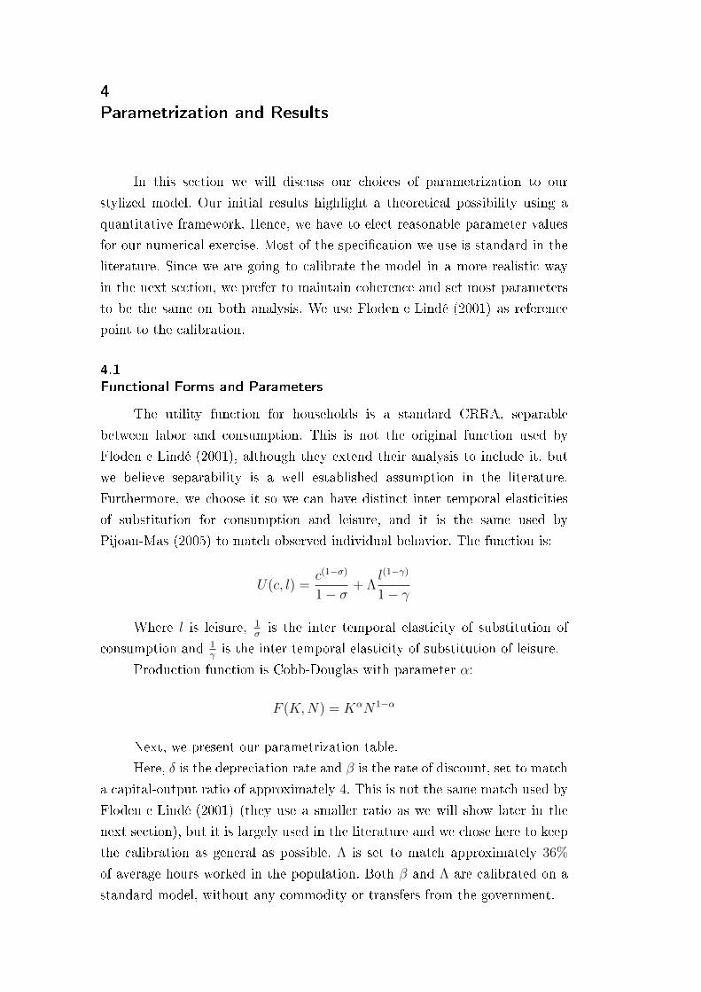
In this section we will discuss our choices of parametrization to our
stylized model. Our initial results highlight a theoretical possibility using a
quantitative framework. Hence, we have to elect reasonable parameter values
for our numerical exercise. Most of the speci�cation we use is standard in the
literature. Since we are going to calibrate the model in a more realistic way
in the next section, we prefer to maintain coherence and set most parameters
to be the same on both analysis. We use Floden e Lindé (2001) as reference
point to the calibration.
4.1
Functional Forms and Parameters
The utility function for households is a standard CRRA, separable
between labor and consumption. This is not the original function used by
Floden e Lindé (2001), although they extend their analysis to include it, but
we believe separability is a well established assumption in the literature.
Furthermore, we choose it so we can have distinct inter temporal elasticities
of substitution for consumption and leisure, and it is the same used by
Pijoan-Mas (2005) to match observed individual behavior. The function is:
U(c, l) =c(1−σ)
1− σ+ Λ
l(1−γ)
1− γ
Where l is leisure, 1σis the inter temporal elasticity of substitution of
consumption and 1γis the inter temporal elasticity of substitution of leisure.
Production function is Cobb-Douglas with parameter α:
F (K,N) = KαN1−α
Next, we present our parametrization table.
Here, δ is the depreciation rate and β is the rate of discount, set to match
a capital-output ratio of approximately 4. This is not the same match used by
Floden e Lindé (2001) (they use a smaller ratio as we will show later in the
next section), but it is largely used in the literature and we chose here to keep
the calibration as general as possible. Λ is set to match approximately 36%
of average hours worked in the population. Both β and Λ are calibrated on a
standard model, without any commodity or transfers from the government.
DBD
PUC-Rio - Certificação Digital Nº 1412607/CA

Chapter 4. Parametrization and Results 25
Table 4.1: Parametrization
Parameters Values Match
γ 2.50σ 1.50
α 0.36Floden and Linde (2001)
δ 0.01
β 0.90 KY≈ 4
Λ 0.70 Average hours worked ≈ 0.36
As for the environment, credit constraint, b, is set to 0 as usual. The
simulated economy is represented by a transition probability matrix of the
idiosyncratic shocks, P , and a productivity set Θ. The arrangement is as
follows:
Table 4.2: States and Stationary Distribution
State θ1 θ2 θ3
Productivity Value 0.1 0.50 1.00
Stationary Mass 44.44% 29.87% 25.78%
Each θ represents a di�erent state of nature with a correspondent productivity value. Eachstate has a correspondent mass of individuals in steady state, represented by percent of totalpopulation.
That means 44.44% of the population in our economy, on the steady
state, will have productivity of θ1 (0.1 according to our parametrization), and
so on. π is the stationary distribution associated with P , and, as we said, that
is important because it will de�ne the mass of households that will receive the
transfers.
Those parameters were chosen to represent a standard developing
economy, and that is why the most productive worker is ten times more
productive than the least, and we have a large fraction of the population with
the lower bound on θ. We will see that the government will choose transfers to
the least productive households only, and still have the majority support. The
commodity parameter, B, is equal to 0.1231. That is an arbitrary value, but
it is set to equal 30% of the GNP in a standard model (without our extension,
just like β and Λ). Of course, the GNP when we add B is di�erent in every
equilibrium, since each one consists in a di�erent value of the transfers, T , and
di�erent eligibility criterion, but that proportion does not varies very much (B
DBD
PUC-Rio - Certificação Digital Nº 1412607/CA

Chapter 4. Parametrization and Results 26
is around 35% of the GNP in most equilibria).
In order to save computational resources, we set the grid of expropriation,
τ , to have only decimal values (10%, 20%, 30% and so on). Although our main
results are unchanged with a �ner grid, we will present results with a �ner grid
later.
The only parameter left to specify is χ, the proportion of political support
the government must achieve to secure power. We de�ne it as being equal
to 50%. This is the most direct value possible for the mass of population
supporting the government, but it is also essentialy arbitrary. The main
mechanism result, meaning the coalition that will be formed between rich
capital holders and poor low productive households, is not likely to change,
however, if we choose another χ.
4.2
Results
On the next �gure we present results for the political support of
the government for various levels of expropriation. Each line represents the
mass of households that support the suggested allocation, when compared
to the outside option equilibrium, when the ruler focus transfers on low
productivity workers only or both low and middle productivity (remember of
the distribution π and the stationary mass in each state). For obvious reasons
we do not need to add a new line representing support when the government
chooses the eligibility criterion to be θ3 (or∞ following our previous notation).
In that case households would be comparing two allocations that only di�er
on the amount transfered, and it is quite evident that nobody would go for
the expropriated economy. The �rst thing that meets the eye is the fact that,
for low values of expropriation, the government can obtain full or almost full
political support even when focusing transfers. In addition, when focusing
transfers on exclusively low productivity households, the government can steal
a larger fraction of B and still maintain power. That is what we call in this
paper, the rise of populism. One can argue that it is not a very good de�nition
of populism, since wealthy households are receiving transfers, as long as they
are in the worse state. That is a fair point, but we must highlight that the mass
of relatively wealthy households among those with the lower productivity is
not very signi�cant. When faced with the urge to expropriate, in our model,
the policy maker will prefer transfers to low productivity households, even
if it is the minority of the population. So populism here rises endogenously
with the solution of our proposed problem, because by targeting speci�c the
poor, the incumbent government can expropriate a fraction of B and still
DBD
PUC-Rio - Certificação Digital Nº 1412607/CA

Chapter 4. Parametrization and Results 27
Figure 4.1: Political Support for each eligibility criterium
Political support for increasing values of expropriation (τ) when transfers are focused on θ1and θ1 + θ2 (44, 44% and 74, 22% of the population respectively)
make the majority better o� than the outside option. Our Political Economic
Equilibrium here would be with τ = 40%, since it is the higher possible value
that maintains over 50% of political support. Although the model is stylized,
and so that value does not say much about real world, it is a considerably high
level of expropriation.
Focused transfers bene�ting households beyond the eligibility criterion
is not new. Berriel e Zilberman (2011), for example, �nd a much higher
proportion of households are happy with Bolsa Familia program in Brazil
than the amount that actual contemplates the program. But the reason it is
possible to target transfers to lower productivity households and still maintain
power are di�erent from the diagnostic given by Berriel e Zilberman (2011).
There, households that were not eligible to the cash transfer program and still
supported it's existence were the poorest among those not contemplated by the
program. The e�ect is an insurance one, since poor workers are more exposed
to the probability of being credit constrained with adverse realizations of the
idiosyncratic shock. In our model, when we analyze which households are better
o� with the populist government (on the Political Economic Equilibrium) with
the ones that would prefer zero expropriation and equal distribution of B,
we �nd that those are the richest fraction of the population. By richest we
mean households that possess more individual capital among those with higher
productivities (and so, not eligible on the optimum). This is not an insurance
e�ect, but a general equilibrium one. In the next table we show how political
support unveils.
The table represents each fraction of the population that supports or
rejects the incumbents allocation. It is divided in percentiles of wealth, meaning
DBD
PUC-Rio - Certificação Digital Nº 1412607/CA

Chapter 4. Parametrization and Results 28
Table 4.3: Political Support and Wealth
Threshold θ / wealth% 0% - 10% 10% - 25% 20% - 50% 50% - 85% 85% - 100%
θ1 Supports Supports Supports Supports Supports
θ2 Rejects Rejects Rejects Supports Supports
θ3 Rejects Rejects Rejects Rejects Supports
Wealth percentiles of total population divided among each productivity state. For eachproductivity state (column) and wealth percentile (line), "Supports" mean the individualsin the respective state (a,θ) is better than on the outside option. "Rejects" means theopposite.
that the �rst column represents the 10% least wealthy households among each
θ, and so on. We can see that support necessary to maintain power in this
populist allocation is actually been given by the wealthiest among those who
does not receive transfers. These results are surprising in a �rst look. Workers
with low capital, even if with high productivity, are more susceptible to being
borrowed constrained in the occurrence of a bad shock. We would expect these
households to prefer an allocation that insure them against these shocks, by
transferring cash directly to them when it happens. But this is not the case
here, since the least wealthy households that are not eligible for transfers are
better o� on the outside option. Households, when faced with the political
decision in matter, have a trade-o�, as always in economics. In one hand they
have an allocation in which they certainly receive transfers, on the other,
they have one that will only pay them in the worst state. To understand
why the richest �nd the latter a better option we must look at two key
macroeconomic variables: interest rates and wages. We can see that interest
rates are consistently higher than on the outside option, and wages are lower.
The reason it is so is due to precautionary savings. Low productivity workers
are credit constrained, and so they must save to consume in the future. Workers
with high productivity choose to save more in precaution against future adverse
shocks, and the possibility of being eventually constrained. When transfers are
directed to worse state of nature, the economy experience a major decrease
in precautionary savings, and consequently capital. This decrease is relative
high when compared to the outside option because we are now transferring
a larger amount. Of course, when τ is too big so that the suggested T is
smaller than no household is better, in fact, the political support decreases
faster than T reaches the outside option level. For example, when τ = 40%
and the government transfer to 74, 22% (θ1 and θ2), the support falls rapidly
to zero because T is now smaller than transfers on the outside option. The
DBD
PUC-Rio - Certificação Digital Nº 1412607/CA

Chapter 4. Parametrization and Results 29
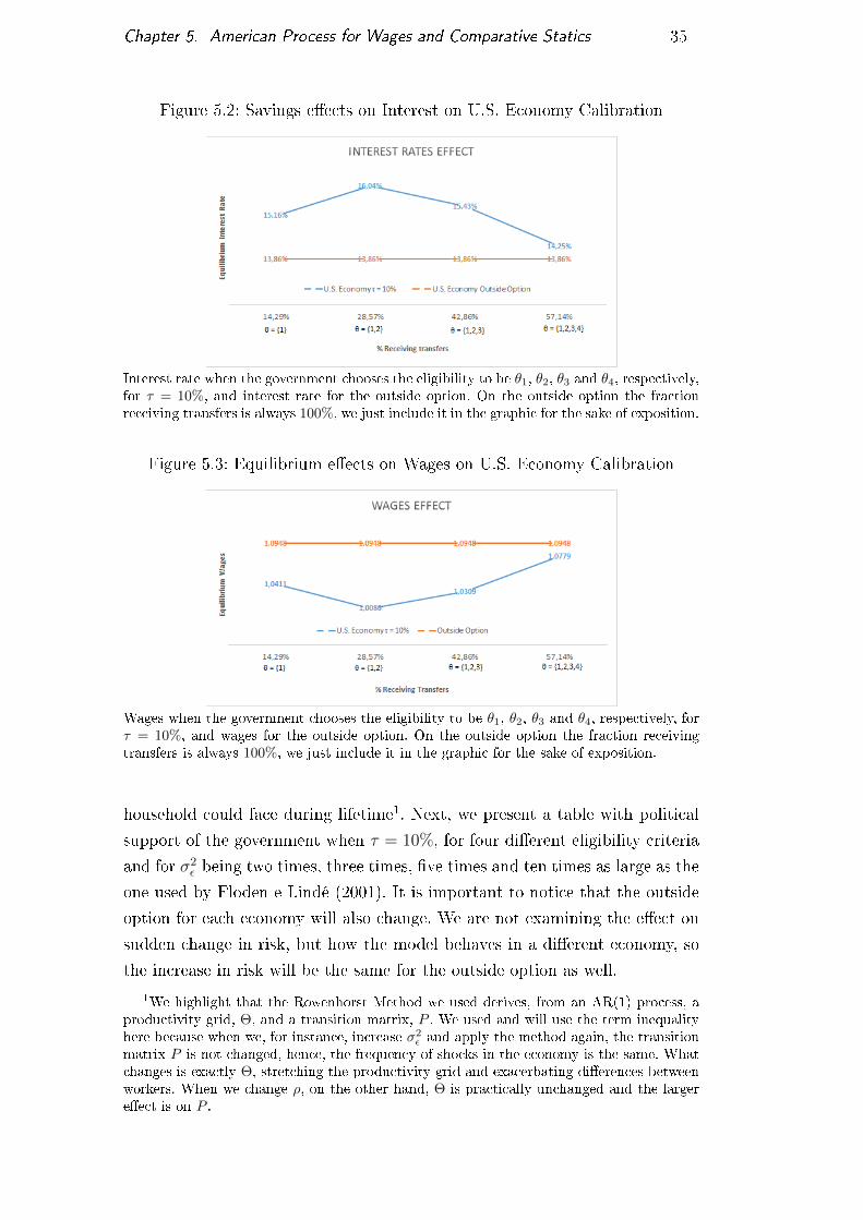
Figure 4.2: Savings e�ects on Interests
For each threshold that de�nes eligibility criterium and each τ that de�nes the amountexpropriated, we present the steady state equilibrium interest rate associated with thatthreshold (mass and state of workers receiving transfers).
Figure 4.3: Equilibrium e�ects on Wages
For each threshold that de�nes eligibility criterium and each τ that de�nes the amountexpropriated, we present the steady state equilibrium wages associated with that threshold(mass and state of workers receiving transfers).
DBD
PUC-Rio - Certificação Digital Nº 1412607/CA

Chapter 4. Parametrization and Results 30
decrease in stationary capital resultant from the precautionary savings e�ect
also a�ects wages, since it positively depends on the former.
Therefore, the trade-o� faced by households that are not eligible for
transfers is a more complex one. They compare an allocation in which they
receive nothing and have a lower salary, although rents on capital are higher,
with another one where they receive some amount and returns on labor are
more attractive, but interests are lower. It is clear now why the mechanism
has the format shown in the table. The e�ects on wages is more relevant to the
most productive households of all, since for them labor income corresponds to
a bigger fraction of total income. Thus, only for extremely wealthy households
the increase in interests is such that they will support the populist allocation.
For the median productivity workers the logic is the same, but they tend
to reject the outside option even with lower accumulated capital, since lower
wages a�ects them relatively less.
Hence, we found that the government, facing the urge to expropriate a
fraction of a national commodity, �nd it optimum to do so by transferring the
remainder to the least productive households in the economy. When he does
it, he obtains the support of those directly bene�ted (the least productive) and
also, via a general equilibrium e�ect on prices, the wealthiest households of the
economy. To the best of our knowledge, this mechanism of political support is
new. In the next section we will test the models prediction with a more realistic
calibration. Also, we perform some comparative statics in key parameters to
share some more light on this mechanism.
DBD
PUC-Rio - Certificação Digital Nº 1412607/CA

5
American Process for Wages and Comparative Statics
On the previous section we used a model with a general parametrization
to highlight a new mechanism of political support of populist governments. We
found that the risk faced by households play a main part in our results, since
the reduction in precautionary savings is the driver of the e�ects responsible for
providing support for the incumbent by those not directly bene�t by populist
policies.
The main issue with this calibration was the process we used for
productivity and, consequently, wages. It is standard in the literature for this
kind of model to assume wages follow an auto regressive process. Of course,
the computation of our model demands this process to be approximated by a
discrete Markov Chain. In this section we will do so, in light of the work by
Floden e Lindé (2001). The point here is to try to address the likelihood of
such coalition in a more fashion calibration.
5.1
U.S. Economy Calibration
Let us assume that the individual productivity is as follows:
θt = exp zt
zt =ρzt−1 + ε
Where ρ < 1 and V ar(ε) = σ2ε . This is similar to the one used
in Floden e Lindé (2001) with the exception that they add a permanent
component. Hence, we can view our model to be a smaller version of theirs,
without ex-ante inequality, only ex-post shocks.
Floden e Lindé (2001) made a very rigorous analysis and estimation of
the parameters ρ and σ2ε . We do not pretend to replicate their estimation.
Instead we borrow their own estimates for the U.S. economy from the period
of 1988 to 1992. They use the Panel Study of Income Dynamics and attempt
to dissociate ex-ante inequality from the ex-post one, by using the supposed
determinants of each one.
For our approximation of that process we use Rowenhorst Method,
since it was shown by Kopecky e Suen (2010) to have desired properties over
Tauchen's famous method. We follow Floden e Lindé (2001) and use 7 states.
DBD
PUC-Rio - Certificação Digital Nº 1412607/CA

Chapter 5. American Process for Wages and Comparative Statics 32
This is important because now the policy maker will be able to focus even
more.
As we said, values for parameters of the utility function and production
we used in our general model were already the same they used in their
speci�cation. We did it so that we could clean the e�ects of most parameters
in the results, and focus on the amount of risk faced by households. As for
internal calibration, Λ is set to match the same 36% average hours worked
in a general economy (without B or T ), but β is set to match a KY
ratio
of 2.6, as Floden e Lindé (2001). It is likely that the value of the discount
play some part in the result, since it a�ects the mass of households with high
accumulated assets in steady state, but again, the model we presented was
supposed to be general and served the purpose of exposing a possible new
mechanism. Our calibration of this section is as follows: We do not include
Table 5.1: U.S. Economy Calibration
Parameters Values Match
ρ 0.9136
σ2ε 0.0426
Floden and Linde (2001)
β 0.85 KY≈ 2.6
Λ 0.70 Average hours worked ≈ 0.36
parameters we use the same value as before for the sake of succinctness. It
is imperative to highlight that with this parametrization the government can
not transfer to less than 50% of the population and still obtain support over
it. The coalition mechanism, although, is still here. As we show in the next
graphic, for τ = 0.10 (which is the smaller possible in our division of the
expropriation grid), he can still obtain support of a mass of workers bigger
than the ones actually receiving transfers. Next we present a table similar to
the one presented in the previous section, where we show political support by
wealth percentiles for the case of τ = 0.10 and transfers for the 14, 29% least
productive in the economy. The table is not so clear as the previous one because
only a very small fraction of the population with high levels of productivity
prefers the populist allocation. What is going on here is that the e�ects on
interests are only compensating the e�ects on wages and the lack of transfers
in all states for extreme wealthy families. The amount of accumulated wealth
needed to support the populist government is so high that only an insigni�cant
mass of households achieves it. All support is being given by the second lowest
in the scale of productivity, because for them, wages are less relevant relatively
DBD
PUC-Rio - Certificação Digital Nº 1412607/CA

Chapter 5. American Process for Wages and Comparative Statics 33
Figure 5.1: Political Mechanism in U.S. Economy Calibration
Political support (vertical) when the government chooses the eligibility to be θ1, θ2, θ3and θ4, respectively (and the mass of workers in each state, on the horizontal axis). Eachfraction of the population receiving transfers in each criterion is equal to the mass of workers,in steady state, on that state and all previous states contemplated.
to rents on capital. We show now graphics representing the general equilibrium
e�ects on interests and wages, as before. The e�ects on interests and wages
are not monotone, and there where no reason for us to think it would be, due
to the high non linearity of this model. It appears that precautionary savings
are at it's peak of reduction when the government transfers to θ1 and θ2, and
we can say so because it is when interests achieve it's maximum value (and
wages it's minimum).
The actual solution to the ruler problem here fails in a sense similar
to our general model. The government can not obtain majority of support
by transferring to a minority. But of course that is highly dependent of
several approximation and parameters chosen here, for example, the number
of productivity states and the grid of τ (we try to change that later). Even
so, apparently the mechanism of political support by capital holders is indeed
weakened when we solved the model for this calibration. When the ruler steals
10% of the commodity and focus transfers to both the least productive and
the two leasts, he obtains only around 3% of additional political support.
That result is not at all discouraging, as we indeed do not expect the U.S.
economy to be highly susceptible to expropriators and populists governments.
It simply states that the American economy is not very likely to experience
the coalition we found to be possible in a general model.
For the sake of completeness, we show now a graphic with a �ner
expropriation grid, where we allow values from the range of 1% to 25%, when
transfers are focused on the bottom two of productivity distribution (θ1 and
θ2, or 28, 57% of the population). We can see that the mechanism does gets
DBD
PUC-Rio - Certificação Digital Nº 1412607/CA

Chapter 5. American Process for Wages and Comparative Statics 34
Table 5.2: Political Support and Wealth in U.S. Calibration
Threshold θ / wealth% 0% - 10% 10% - 66% 66% - 99.99% 100%
θ1 Supports Supports Supports Supports
θ2 Rejects Rejects Supports Supports
θ3 Rejects Rejects Rejects Supports
θ4 Rejects Rejects Rejects Supports
θ5 Rejects Rejects Rejects Supports
θ6 Rejects Rejects Rejects Supports
θ7 Rejects Rejects Rejects Supports
Wealth percentiles of total population divided among each productivity state. For eachproductivity state (column) and wealth percentile (line), "Supports" mean the individualsin the respective state (a,θ) is better than on the outside option. "Rejects" means theopposite.
stronger for low values of τ . That is expected since any e�ect arising from the
transfers should get more pronounced if this transfers are higher. But is not
su�cient to hold the results as we said. If we increase the eligibility criterion
even further, the mechanism gets even weaker because we are dividing the
same amount more times and the e�ects are mitigated.
5.2
Comparative Statics on Wages Process
So in which kind of economy such an arrangement is more likely to occur?
In order to try addressing this question we performed some comparative statics
for the AR(1) process for individual income. All tables and graphics we will
show are relative to τ = 10%. In other words, we do not solve all of the problem
for every di�erent value of each parameter in search for the political economic
equilibrium as we did in our general model, for that would be extremely time
consuming. And again, the existence or not of a political economic equilibrium
in the sense we proposed, with τ > 0, is not of main importance here since it
will depend on aspects of the model that do not share direct resemblance with
reality. The point in doing comparative statics here is just try to understand
how the strength of the mechanism can vary with the amount of uncertainty
faced by households.
Changing σ2ε The most direct measure of risk is of course σ2
ε . It changes
the degree of inequality in the economy, as it determines the magnitude of
the idiosyncratic shocks and, therefore, a�ects the productivity changes a
DBD
PUC-Rio - Certificação Digital Nº 1412607/CA
Chapter 5. American Process for Wages and Comparative Statics 35
Figure 5.2: Savings e�ects on Interest on U.S. Economy Calibration
Interest rate when the government chooses the eligibility to be θ1, θ2, θ3 and θ4, respectively,for τ = 10%, and interest rate for the outside option. On the outside option the fractionreceiving transfers is always 100%, we just include it in the graphic for the sake of exposition.
Figure 5.3: Equilibrium e�ects on Wages on U.S. Economy Calibration
Wages when the government chooses the eligibility to be θ1, θ2, θ3 and θ4, respectively, forτ = 10%, and wages for the outside option. On the outside option the fraction receivingtransfers is always 100%, we just include it in the graphic for the sake of exposition.
household could face during lifetime1. Next, we present a table with political
support of the government when τ = 10%, for four di�erent eligibility criteria
and for σ2ε being two times, three times, �ve times and ten times as large as the
one used by Floden e Lindé (2001). It is important to notice that the outside
option for each economy will also change. We are not examining the e�ect on
sudden change in risk, but how the model behaves in a di�erent economy, so
the increase in risk will be the same for the outside option as well.
1We highlight that the Rowenhorst Method we used derives, from an AR(1) process, aproductivity grid, Θ, and a transition matrix, P . We used and will use the term inequalityhere because when we, for instance, increase σ2
ε and apply the method again, the transitionmatrix P is not changed, hence, the frequency of shocks in the economy is the same. Whatchanges is exactly Θ, stretching the productivity grid and exacerbating di�erences betweenworkers. When we change ρ, on the other hand, Θ is practically unchanged and the largere�ect is on P .
DBD
PUC-Rio - Certificação Digital Nº 1412607/CA

Chapter 5. American Process for Wages and Comparative Statics 36
Table5.3:
Com
parativeStatics
onσ2 ε
τ=
10%
Political
Support
%ReceivingTransfers
Threshold
Standard
σ2 ε
=0.
052
σ2 ε
=0.
1278
σ2 ε
=0.
213
σ2 ε
=0.
426
14.29%
θ=
117.02%
16.35%
16.45%
17.45%
21.83%
28.57%
θ=
1,2
31,97%
33.87%
35.15%
35.93%
38.14%
42.86%
θ=
1,2,
343.32%
43.68%
44.09%
44.40%
43.83%
57.14%
θ=
1,2,
3,4
57.14%
57.15%
57.17%
57.19%
57.14%
Each
fractionofthepopulationreceivingtransfersiscorrespondentto
aneligibilitycriterion(fromθ 1
toθ 4).Thetable
show
sthepercentageofthepopulation
betterthantheonoutsideoutsideoptionforincreasingvalues
ofσ2 ε(twiceaslargeto
tentimes
aslarge).
DBD
PUC-Rio - Certificação Digital Nº 1412607/CA
Chapter 5. American Process for Wages and Comparative Statics 37
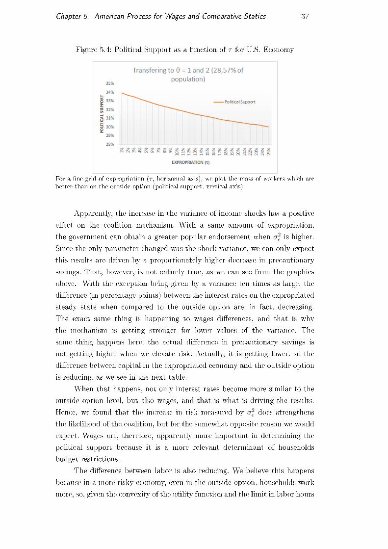
Figure 5.4: Political Support as a function of τ for U.S. Economy
For a �ne grid of expropriation (τ , horizontal axis), we plot the mass of workers which arebetter than on the outside option (political support, vertical axis).
Apparently, the increase in the variance of income shocks has a positive
e�ect on the coalition mechanism. With a same amount of expropriation,
the government can obtain a greater popular endorsement when σ2ε is higher.
Since the only parameter changed was the shock variance, we can only expect
this results are driven by a proportionately higher decrease in precautionary
savings. That, however, is not entirely true, as we can see from the graphics
above. With the exception being given by a variance ten times as large, the
di�erence (in percentage points) between the interest rates on the expropriated
steady state when compared to the outside option are, in fact, decreasing.
The exact same thing is happening to wages di�erences, and that is why
the mechanism is getting stronger for lower values of the variance. The
same thing happens here: the actual di�erence in precautionary savings is
not getting higher when we elevate risk. Actually, it is getting lower, so the
di�erence between capital in the expropriated economy and the outside option
is reducing, as we see in the next table.
When that happens, not only interest rates become more similar to the
outside option level, but also wages, and that is what is driving the results.
Hence, we found that the increase in risk measured by σ2ε does strengthens
the likelihood of the coalition, but for the somewhat opposite reason we would
expect. Wages are, therefore, apparently more important in determining the
political support because it is a more relevant determinant of households
budget restrictions.
The di�erence between labor is also reducing. We believe this happens
because in a more risky economy, even in the outside option, households work
more, so, given the convexity of the utility function and the limit in labor hours
DBD
PUC-Rio - Certificação Digital Nº 1412607/CA

Chapter 5. American Process for Wages and Comparative Statics 38
Figure 5.5: σ2ε and Interest Rates in Equilibrium
For each eligibility criterion (from θ1 to θ4, horizontal axis, for τ = 10%) the graphic showsthe di�erence, in percentage points, between the interest rate on the referred equilibriumand the one on the outside option equilibrium.
Figure 5.6: σ2ε and Wages in Equilibrium
For each eligibility criterion (from θ1 to θ4, horizontal axis, for τ = 10%) the graphic showsthe percentual di�erence between wages on the referred equilibrium and the one on theoutside option equilibrium.
DBD
PUC-Rio - Certificação Digital Nº 1412607/CA

Chapter 5. American Process for Wages and Comparative Statics 39
Table5.4:σ2 εandCapital
inEquilibrium
τ=
10%
Political
Support
%ReceivingTransfers
Threshold
Standard
σ2 ε
=0.
052
σ2 ε
=0.
1278
σ2 ε
=0.
213
σ2 ε
=0.
426
14.29%
θ=
12.02
-2.55%
2.55
-1.66%
3.15
1.36%
4.43
-0.71%
9.11
-0.94%
28.57%
θ=
1,2
1.82
-12.14%
2.31
-11.14%
2.86
-7.97%
4.12
-7.61%
8.82
-4.02%
42.86%
θ=
1,2,
31.92
-7.10%
2.36
-8.86%
2.915
6.42%
4.16
-6.63%
8.96
-2.58%
57.14%
θ=
1,2,
3,4
2.11
1.74%
2.54
-2.08%
3.10
-0.22%
4.37
-2.02%
9.25
0.66%
Thetable
show
s,foreach
eligibilitycriterion,thesteadystate
amountofcapitalonthereferred
equilibrium,andthepercentualdi�erentbetweenthatamount
andtheoutsideoptionone.
DBD
PUC-Rio - Certificação Digital Nº 1412607/CA

Chapter 5. American Process for Wages and Comparative Statics 40
o�ered, the percentage di�erence tends to fall. We solved the same model with
exogenous supply of labor and found that the mechanism gets even stronger.
That happens because the di�erences in labor supply and demand partially
o�sets the di�erence in wages. When labor is exogenous, wages di�erences are
reduced proportionately more.
Also, we believe the sudden increase in interest rate percentage points
when σ2ε is ten times larger than the American one can be a scale e�ect. When
we change σ2ε and apply Rowenhorst's Method we basically change Θ, the
grid of productivity, increasing the inequality of the economy. That change,
of course, a�ects the absolute level of labor and, although this is partially
controlled by the similar change in outside option, the percentage changes can
be more drastic here. Truly, the complexity of the model and the fact that it
is a general equilibrium one, where variables are altogether determined, make
it very hard for us to explain minutely every aspect of it.
Changing ρ First of all, ρ is not a direct measure of risk in an economy.
It simply represents the persistence of the shocks. On one hand, if we decrease
the value of ρ, an individual has a higher chance of becoming poor when rich,
on the other, a low productive household has a higher chance of becoming
productive overnight. It is, therefore, ambiguous. The motivation for this
comparative statics is to analyze how a degree of social changes in an economy
correlates with our mechanism of political support. If when we change σ2ε we
only change inequality (meaning the di�erence between the most productive
and the least), when we change ρ we a�ect very little the productivity grid Θ.
The major changes are on the derived transition matrix P . And although we
can not properly say we are increasing risk in the economy, households will
be experiencing sharper changes in income, and so we would expect them to
accumulate more assets for protection. That is indeed the case. But �rst, we
show the table for political support when ρ is 90%, 85% and 80% of the value it
takes in the American economy (note that we are not using the values ρ = 0.9,
ρ = 0.85 and ρ = 0.8, but instead we chose to represent smaller values of the
parameter as proportion of the one used by Floden e Lindé (2001)).
The results are not what we would expect at �rst, but are in line
with the ones we showed when changing σ2ε . To see why, take a look at the
e�ects on interests and wages. Indeed, as we said, precautionary savings
decreases proportionately more when shocks are more transient. Di�erences
in accumulated capital are higher when the government focus transfers to low
productivity workers in an economy where the persistence in income is lower,
and that is why di�erences in interests are higher. But is also true in that case
that wages are lower, as we can see from the �gure. As before, wages appear to
DBD
PUC-Rio - Certificação Digital Nº 1412607/CA

Chapter 5. American Process for Wages and Comparative Statics 41
Table5.5:
Com
parativeStatics
onσ2 εwithExogenousLabour
τ=
10%
Political
Support
%ReceivingTransfers
Threshold
Standard
σ2 ε
=0.
052
σ2 ε
=0.
1278
σ2 ε
=0.
213
σ2 ε
=0.
426
14.29%
θ=
115.29%
15.69%
16.31%
18.42%
24.64%
28.57%
θ=
1,2
30.22%
30.91%
31.92%
35.36%
41.00%
42.86%
θ=
1,2,
343.05%
43.77%
44.36%
45.11%
47.75%
57.14%
θ=
1,2,
3,4
57.14%
57.14%
57.14%
57.14%
57.14%
Each
fractionofthepopulationreceivingtransfersiscorrespondentto
aneligibilitycriterion(fromθ 1
toθ 4).Thetable
show
sthepercentageofthepopulation
betterthantheonoutsideoutsideoptionforincreasingvalues
ofσ2 ε(twiceaslargeto
tentimes
aslarge).
DBD
PUC-Rio - Certificação Digital Nº 1412607/CA

Chapter 5. American Process for Wages and Comparative Statics 42
Figure 5.7: ρ and Interest Rates in Equilibrium
For each eligibility criterion (from θ1 to θ4, for τ = 10%) the graphic shows the di�erence,in percentage points, between the interest rate on the referred equilibrium and the one onthe outside option equilibrium.
Figure 5.8: ρ and Wages in Equilibrium
For each eligibility criterion (from θ1 to θ4, for τ = 10%) the graphic shows the percentualdi�erence between wages on the referred equilibrium and the one on the outside optionequilibrium.
DBD
PUC-Rio - Certificação Digital Nº 1412607/CA
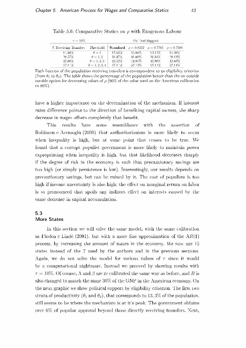
Chapter 5. American Process for Wages and Comparative Statics 43
Table 5.6: Comparative Statics on ρ with Exogenous Labour
τ = 10% Political Support
% Receiving Transfers Threshold Standard ρ = 0.8222 ρ = 0.7765 ρ = 0.7308
14.29% θ = 1 17.02% 15.98% 14.74% 14.46%28.57% θ = 1, 2 31.97% 31.00% 29.84% 29.12%42.86% θ = 1, 2, 3 43.32% 42.97% 42.89% 42.86%57.14% θ = 1, 2, 3, 4 57.14% 57.14% 57.14% 57.14%
Each fraction of the population receiving transfers is correspondent to an eligibility criterion(from θ1 to θ4). The table shows the percentage of the population better than the on outsideoutside option for decreasing values of ρ (90% of the value used on the American calibrationto 80%).
have a higher importance on the determination of the mechanism. If interest
rates di�erence points to the direction of bene�ting capital owners, the sharp
decrease in wages o�sets completely that bene�t.
This results bare some resemblance with the assertion of
Robinson e Acemoglu (2006) that authoritarianism is more likely to occur
when inequality is high, but at some point that ceases to be true. We
found that a corrupt populist government is more likely to maintain power
expropriating when inequality is high, but that likelihood decreases sharply
if the degree of risk in the economy is such that precautionary savings are
too high (or simply persistence is low). Interestingly, our results depends on
precautionary savings, but can be ruined by it. The cost of populism is too
high if income uncertainty is also high: the e�ect on marginal return on labor
is so pronounced that spoils any indirect e�ect on interests caused by the
same decrease in capital accumulation.
5.3
More States
In this section we will solve the same model, with the same calibration
as Floden e Lindé (2001), but with a more �ne approximation of the AR(1)
process, by increasing the amount of states in the economy. We now use 15
states instead of the 7 used by the authors and in the previous sections.
Again, we do not solve the model for various values of τ since it would
be a computational nightmare. Instead we proceed by showing results with
τ = 10%. Of course, Λ and β are re calibrated the same way as before, and B is
also changed to match the same 30% of the GNP in the American economy. On
the next graphic we show political support by eligibility criterion. The �rst two
strata of productivity (θ1 and θ2), that corresponds to 13, 3% of the population,
still seems to be where the mechanism is at it's peak. The government obtains
over 6% of popular approval beyond those directly receiving transfers. Next,
DBD
PUC-Rio - Certificação Digital Nº 1412607/CA
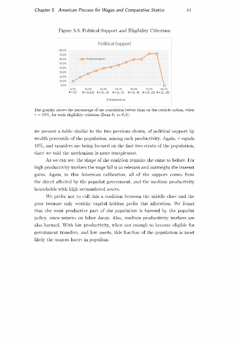
Chapter 5. American Process for Wages and Comparative Statics 44
Figure 5.9: Political Support and Eligibility Criterium
The graphic shows the percentage of the population better than on the outside option, whenτ = 10%, for each eligibility criterion (from θ1 to θ13).
we present a table similar to the two previous shown, of political support by
wealth percentile of the population, among each productivity. Again, τ equals
10%, and transfers are being focused on the �rst two strata of the population,
since we said the mechanism is more conspicuous.
As we can see, the shape of the coalition remains the same as before. For
high productivity workers the wage fall is to relevant and outweighs the interest
gains. Again, in this American calibration, all of the support comes from
the direct a�ected by the populist government, and the medium productivity
households with high accumulated assets.
We prefer not to call this a coalition between the middle class and the
poor because only wealthy capital holders prefer this allocation. We found
that the most productive part of the population is harmed by the populist
policy, since returns on labor decay. Also, medium productivity workers are
also harmed. With low productivity, when not enough to become eligible for
government transfers, and low assets, this fraction of the population is most
likely the utmost losers in populism.
DBD
PUC-Rio - Certificação Digital Nº 1412607/CA

Chapter 5. American Process for Wages and Comparative Statics 45
Table5.7:
Political
Supportwith15
states
Thresholdθ/wealth%
0%-10%
10%
-20%
20%
-78%
78%
-99.7%
99.97%
-99.99%
100.00%
θ1Supports
Supports
Supports
Supports
Supports
Supports
θ2Supports
Supports
Supports
Supports
Supports
Supports
θ3Rejects
Supports
Supports
Supports
Supports
Supports
θ4Rejects
Reject
Supports
Supports
Supports
Supports
θ5Rejects
Reject
Reject
Reject
Supports
Supports
θ6Rejects
Reject
Reject
Reject
Reject
Supports
θ7Rejects
Reject
Reject
Reject
Reject
Supports
θ8Rejects
Reject
Reject
Reject
Reject
Supports
θ9Rejects
Reject
Reject
Reject
Reject
Supports
θ10
Rejects
Reject
Reject
Reject
Reject
Supports
θ11
Rejects
Reject
Reject
Reject
Reject
Supports
θ12
Rejects
Reject
Reject
Reject
Reject
Supports
θ13
Rejects
Reject
Reject
Reject
Reject
Supports
θ14
Rejects
Reject
Reject
Reject
Reject
Supports
θ15
Rejects
Reject
Reject
Reject
Reject
Supports
Wealthpercentilesoftotalpopulationdivided
amongeach
productivitystate.Foreach
productivitystate
(column)andwealthpercentile(line),"Supports"
mean
theindividualsin
therespectivestate
(a,θ)isbetterthanontheoutsideoption."Rejects"meanstheopposite.
DBD
PUC-Rio - Certificação Digital Nº 1412607/CA

6
Final Remarks
We tried to address a few questions about the dynamics of expropriation
and power on developing countries. We have various examples of left oriented
governments that even though expropriating private �rms and causing,
sometimes, major economics di�culties still maintains power by popular
support. We found that populism can be a response to the desire to appropriate
of a fraction of a commodity, and, therefore, is more likely that a corrupt
government (for example) chooses populist politics in order to hold o�ce.
Interestingly, the part of the population that supports the expropriator,
but populist, government, besides of course the low productive households
(bene�ted directly by the populism policy), is the elite. That comes from
a general equilibrium e�ect on interest rate, caused by the contraction on
precautionary savings in the economy, possible due to the transfers households
receive when in bad states in political equilibrium. Individuals that are not
directly a�ected by populists policies compare an allocation in which they
receive nothing from the government and have a lower salary, although rents
on capital are higher, with another one where they receive some amount and
returns on labor are more attractive, but interests are lower. We found that
for some parametrization it is possible that the increase in interests o�sets
the reduction in salaries and absence of transfers, so that a coalition is formed.
Poor, low productivity households and rich capital owners support the populist
allocation instead of an egalitarian one.
Also, we calibrated our model to an American economy like in
Floden e Lindé (2001) and found that the mechanism is weak in this more
realistic case. Further, we performed some comparative statics in parameters
of the AR(1) process we used for wages to try understanding in which types of
economy our found arrangement is more likely to occur. We found that when
inequality rises the mechanism gets stronger because the reduction in wages
falls. We also found that if persistence of income shocks are low, the coalition
looses likelihood. Too much precautionary savings increases the negative e�ects
on wages and that o�sets the higher di�erences in interest rates. Precautionary
savings are, at the same time, the driver and the ruin of our result.
DBD
PUC-Rio - Certificação Digital Nº 1412607/CA

Bibliography
ABREY, D.; PEARCE, D. ; STACCHETTI, E.. Toward a Theory
of Discounted Repeated Games with Imperfect Monitoring.
Econometrica, 58(5):1041�1063, September 1990.
ACEMOGLU, D.; ROBINSON, J. A.. A theory of political transitions. The
American Economic Review, 91(4):938�963, September 2001.
ROBINSON, J. A.; ACEMOGLU, D.. Economic Origins of Dictatorship
and Democracy. Cambridge University Press, Cambridge, UK, 2006.
ACEMOGLU, D.; VINDIGNI, A. ; TICCHI, D.. Emergence and Persistence
of Ine�cient States. Journal of the European Economic Association,
9(2):177�208, April 2011.
ACEMOGLU, D.; EGOROV, G. ; SONIN, K.. A Political Theory of
Populism. The Quarterly Journal of Economics, pp 771�805, December 2013.
AGUIAR, M.; AMADOR, M. ; GOPINATH, G.. Investment Cycles and
Sovereign Debt Overhang. The Review of Economic Studies, 76(1):1�31,
January 2009.
AGUIAR, M.; AMADOR, M.. Growth in the Shadow of Expropriation.
The Quarterly Journal of Economics, (126):651�697, 2011.
AIYAGARI, S. R.. Uninsured Idiosyncratic Risk and Aggregate Saving.
The Qua, 109(3):659�684, August 1994.
AMADOR, M.. A Political Economy Model of Sovereign Debt
Repayment. Job Market Paper, 2002.
ARELLANO, C.. Default Risk and Income Fluctuations in Emerging
Economies. American Economic Review, 98(3):690�712, June 2008.
BARRO, R. J.. Determinants of Democracy. Journal of Political Economy,
107(S6):158�183, December 1999.
BERRIEL, T. C.; ZILBERMAN, E.. Targeting the Poor: A
Macroeconomic Analysis of Cash Transfer Programs. December 2011.
BULLOW, J.; ROGOFF, K.. Sovereign Debt: Is to Forgive to Forget?
American Economic Review, 79(1):43�50, March 1989.
DBD
PUC-Rio - Certificação Digital Nº 1412607/CA
Bibliography 48
CHAMLEY, C.. Optimal Taxation of Capital Income in General
Equilibrium with In�nite Lives. Econometrica, 54(3):607�622, May 1986.
CORBAE, D.; D'ERASMO, P. ; KURUSCU, B.. Politico-Economic
Consequences of Rising Wage Inequality. Journal of Monetary
Economics, (56):43�61, 2009.
DOS REIS, A. C.; ZILBERMAN, E.. The insurance role of public
employment. September 2014.
FLODEN, M.; LINDÉ, J.. Idiosyncratic risk in the united states and
sweden: Is there a role for government insurance? Review of Economic
dynamics, 4(2):406�437, 2001.
FLODEN, M.. The e�ectiveness of government debt and transfers as
insurance, 2001.
KLETZER, K.; WRIGHT, B.. Sovereign Debt as Intertemporal Barter.
American Economic Review, 90(3):621�639, June 2000.
KOPECKY, K. A.; SUEN, R. M.. Finite state markov-chain
approximations to highly persistent processes. Review of Economic
Dynamics, (13):701�714, March 2010.
KRUSSEL, P.; RIOS-RULL, J.-V.. What Constitutions Promote Capital
Accumulation? A Political-Economy Approach. December 1994.
KRUSSEL, P.; QUADRINI, V. ; RIOS-RULL, J.-V.. Politico-Economic
Equilibrium and Economic Growth. Journal of Economic Dynamics and
Control, (21):243�272, 1997.
KRUSSEL, P.; RIOS-RULL, J.-V.. On the Size of U.S. Government:
Political Economy in the Neoclassical Growth Model. The American
Economic Review, 89(5):1156�1181, December 1999.
KRUSSEL, P.; MUKOYAMA, T.; SAHIN, A. ; SMITH JR., A. A.. Revisiting
the welfare e�ects of eliminating business cycles. Review of Economic
Dynamics, (12):393�404, 2009.
MAZZUCA, S. L.. The Rise of Rentier Populism. Journal of Democracy,
24(2), April 2013.
MELTZER, A. H.; RICHARD, S. F.. A Rational Theory of the Size of
Government. The Journal of Political Economy, 89(5):914�927, October 1981.
DBD
PUC-Rio - Certificação Digital Nº 1412607/CA

Bibliography 49
PIJOAN-MAS, J.. Precautionary savings or working longer hours?
November 2005.
BESLEY, T.; PERSSON, T.. Pillars of prosperity: The political
economics of development clusters. Princeton University Press, 2011.
RIOS-RULL, J.-V.. Computation of equilibria in heterogenous agent
models. Federal Reserve Bank of Minneapolis Research Department Sta� Report
231, May 1997.
LJUNGQVIST, L.; SARGENT, T. J.. Recursive Macroeconomic Theory,
chapter 18, pp 728�729. Massachusetts Institute of Technology, 3 edition, 2012.
THOMAS, J.; WORRAL, T.. Foreign Direct Investment and the Risk
of Expropriation. Review of Economics Studies, 61:81�108, 1994.
WERNING, I.. Optimal Fiscal Policy with Redistribution. The Quarterly
Journal of Economics, pp 925�967, August 2007.
STRAUB, L.; WERNING, I.. Positive Long Run Capital Taxation:
Chamley-Judd Revisited. NBER Working Paper No. 20441, August 2014.
ACEMOGLU, D.; ROBINSON, J. A.. Why Did the West Extend
the Franchise? Democracy, Inequality, and Growth in Historical
Perspective. The Quarterly Journal of Economics, 115(4):1167�1199,
November 2000.
WRIGHT, M.. Reputations and Sovereign Debt. Manuscript, Stanford
University, September 2002.
DE SOUZA, G. M.. Design Otimo e Aspectos Politicos do Bolsa
Familia. VII Premio SOF de Monogra�as. Tema 1: Qualidade do Gasto Publico.
DBD
PUC-Rio - Certificação Digital Nº 1412607/CA

A
Appendix
Computation
We use standard algorithms known in the literature to �nd our stationary
competitive equilibriums, found in Rios-Rull (1997). We actually use a
slight variation of the �xed point capital iteration method, also found in
Ljungqvist e Sargent (2012). The general algorithm is as follows:
1. Discretize the individual capital grid [b, a1, a2, ..., an], the grid of τ ,
[τ1, τ2, ..., τs] and the productivity grid [θ1, θ2, ..., θm];
2. For each τ i ∈ [τ1, τ2, ..., τs] and θi ∈ [θ1, θ2, ..., θm]:
� Calculate the correspondent T (remember, T only depends on the
distribution among the productivity state and we know that from the
transition probability matrix P );
� Iterate to �nd the competitive equilibrium:
� Guess a lower bound and an upper bound for the interest rate and
build an equally divided grid, say, with 3 rates {rl, rm, ru} whererm is the median (you can build this grid larger, in fact, through
our work we used 4, but 3 is the least);� For each r ∈ {rl, rm, ru}, plot the correspondent per capita capital
demand {kdl , kdm, kdu} and wages {wl, wm, wu};� For each r and w in the grid, plot the per capita capital o�er
{kol , kom, kou} by solving the agents problem:
∗ Use any algorithm to �nd g(a, θ) and n(a, θ) (we used standard
value function iteration);∗ Find the correspondent stationary distribution λ(a, θ);∗ Determine the aggregate capital K =
∫g(a, θ)dλ(a, θ) and
labor N =∫θn(a, θ)dλ(a, θ);
� Compare the per capita capital o�er and demand for each r on
the grid to �nd the interval where demand intercepts with o�er.
In other words, �nd {r2l , r2u} on the grid of r so that the a new
grid built by subtracting the o�er grid by the demand grid changes
signal ({{kdl − kol , kdm − kom, kdu − kou}});� Use {r2l , r2u} as your new upper and lower bounds for r and repeat
the process until |riu − ril | < ε for some tolerance parameter ε;
DBD
PUC-Rio - Certificação Digital Nº 1412607/CA

Appendix A. Appendix 51
� Having the stationary value functions you can now determine the mass
of workers happier when compared to the outside option;
3. Repeat the process for each τ i ∈ [τ1, τ2, ..., τs] and θi ∈ [θ1, θ2, ..., θm] and
take the higher τ so that a mass of χ workers are better o�. That is your
political economic equilibrium.
Note that this process also �nds the outside option, since you can simply
set the �rst τ in the grid to be 0. The �xed point iteration we used in bound to
converge if the initial guess on upper and lower bound contains the equilibrium
interest rate.
It is important to emphasize that the stationary distribution used to
determine the mass of workers better than the outside option is the suggested
allocation one. We basically �nd the points in the state space grid (a, θ) where
V (a, θ; τ i, T, θi) > V (a, θ; 0, T ,∞) and then use λ(a, θ; τ i, θ
i) to compute the
mass.
DBD
PUC-Rio - Certificação Digital Nº 1412607/CA