MapReduce“Divide and Conquer”

CONTENTS

1. ABSTRACT

2. INTRODUCTION

3. PROGRAMMING MODEL

4. IMPLEMENTATION

5. REFINEMENTS

6. PREFORMANCE

7. EXPERIENCE

8. RELATED WORK

9. CONCLUSION

ABSTRACT

• MapReduce is a model used to analyze large amounts of data

• Map creates key:value pairs, irrespective of duplicates

• Reduce takes the key-value pairs created by the Map function and condenses them down to remove duplicate results

• Processing and generating large data sets.

• Real world tasks

• Run-time system that takes care of details partitioning the input data

• Implementation on a large cluster of commodity machines

1. INTRODUCTION• Computations have been written to process documents, web logs,

and raw data

• Distributed across hundreds or thousands of machines in order to finish in a reasonable amount of time

• Designed a new abstraction that allows us to express the simple computations

• Google developed an abstraction to allow users run distributed computations without knowing about distributed computing

• Hides the messy details of parallelization, fault-tolerance, data distribution, and load balancing

• MapReduce interface tailored towards our cluster-based computing environment

• Simple and powerful interface.

2. PROGRAMMING MODEL

• Map() and Reduce()

• MapReduce library groups together intermediate values associated with same intermediate key I

• Passes values to Reduce() via an iterator

• Reduce() merges values to form possibly smaller set of values

• Zero or one output value is produced per Reduce invocation

2.1 EXAMPLE Counting Number of Word Occurrences (user code)

map (String key, String value):// key: document name// value: document contents// emits each word plus associated count of occurrences

for each word w in value:EmitIntermediate (w, “1”);

reduce (String key, Iterator values):// key: a word// values: a list of counts// sums together all counts emitted for a particular word

int result = 0;for each v in values:result += ParseInt(v);Emit (AsString(result));

user code is linked together with the MapReduce library

2.1 ASSOCIATED TYPES

map (k1, v1) list (k2, v2)

reduce (k2, list (v2)) list (v2)

• Input keys & values drawn from a different domain than the output keys & values

• Intermediate keys & values are from the same domain as the output keys & values

• User code to convert between strings & appropriate types

2.3 MORE EXAMPLESMap() Reduce()

Distributed Grep Emits a line if matches supplied pattern

Identity fnc that copies the supplied intermediate data to output

Count of URL Access Frequency

Processes logs of web page requests & outputs(URL, 1)

Adds together all values for the same URL and emits a (URL, total cnt) pair

Reverse Web-Link Graph Outputs (target, source) pairs for each link to a target URL found in page named source

Concatenates the list of all source URLs assoc. with given target URL and emits the pair: (target, list(source))

Term-Vector per Host Term vector summarizes most important words that occur in document as list of (word, frequency) pairs

Emits a (hostname, term vector) pair for each input document where host name is extracted from URL of the document

Inverted Index Parses each document, and emits a sequence of (word, document ID) pairs

Accepts all pairs for a given word, sorts the corresponding document ID’s & emits a(word, list(document ID)) pair. Set of all output forms simple inverted index.

Distributed Sort Extracts the key from each record, and emits a (key, record) pair

Emits all pairs unchanged

3. IMPLEMENTATION

• The right choice depends on the environment

• Google’s setup

• typically dual x86 processors 2-4GB memory

• 100Mb/s or 1Gb/s networking hardware

• Hundreds or thousands of machines per cluster

• Inexpensive IDE disks directly on machines

3.1 EXECUTION• Input data partitioned into M splits

• Intermediate key space partitioned into R pieces.

1. Splits input files into 16 to 64 MB per piece.

2. Master assigns tasks.

3. Worker reads the input split.

4. Buffered pairs get written to local disk.

5. Reduce worker makes procedure call to retrieve data from map worker’s local disk.

6. Results are written to final output file

7. Master wakes user program and returns all output files.

EXECUTION(Cont.)

3.2 MASTER DATA STRUCTURES

3.3 FAULT TOLERANCE

3.4 LOCALITY

• Due to low network capacity data is stored on the local disk of each machine

• The files are split into 64MB blocks. Each block is copied three times to other machines

• The master machine tries to schedule jobs on the machine that contains the data.

• Otherwise, it schedules a job close to a machine containing the job data

• It’s possible that a job may use no network bandwidth

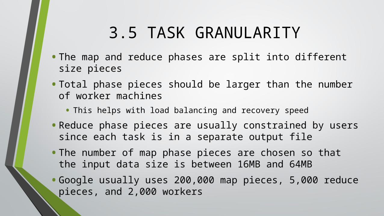
3.5 TASK GRANULARITY

• The map and reduce phases are split into different size pieces

• Total phase pieces should be larger than the number of worker machines

• This helps with load balancing and recovery speed

• Reduce phase pieces are usually constrained by users since each task is in a separate output file

• The number of map phase pieces are chosen so that the input data size is between 16MB and 64MB

• Google usually uses 200,000 map pieces, 5,000 reduce pieces, and 2,000 workers

3.6 BACKUP TASKS• “Straggler” machines can cause large total computation time

• Stragglers can be caused by many different reasons

• Straggler alleviation is possible

• The master backs up in-progress tasks when the operation is close to finishing

• Task is marked as complete when the primary task or backup completes

• Backup task overhead has been tuned to a couple percent

• An example task takes 44% longer when the backup is disabled

4. REFINEMENTS

• General algorithms fit most needs

• User defined Tweaks to the Map and Reduce functions fit special problems

4.1 PARTITIONING FUNCTION

• Users can define the number of reduce tasks to run (R)

• We can redefine the intermediate keys

• A default function is hash(key) mod R

• Sometimes we may want to group output together, such as grouping web data by domain

• We can redefine partition to use hash(Hostname(urlkey)) mod R

4.2 ORDERING GUARANTEE

• Within each partition, intermediate key/value pairs are always processed in increasing order

• This supports efficient lookup of random keys

4.3 CONTROL FUNCTION

• There is sometimes significant repetition in the intermediate keys

• This is usually handled in the Reduce function, but sometimes we want to partially combine it in the Map function

• The combiner function does this for us, and in some situations grants significant performance gains

4.4 INPUT AND OUTPUT TYPE

• MapReduce can take data from a number of formats

• The way the data is organized for input greatly effects the output

• Adding support for a new data type only requires users to change the reader interface

4.5 SIDE EFFECTS

• Sometimes we want to output additional files from the Map or Reduce functions

• Users are responsible for these files, as long as these outputs are deterministic

4.6 SKIPPING BAD RECORDS

• Sometimes there are bugs in user code

• Course of action is to fix the bug

• It is acceptable to ignore a few records

• Optional mode of execution

• Detects which records cause deterministic crashes and skips them

4.7 LOCAL EXECUTION

• Debugging problems can be tricky

• Decisions can be made dynamically by the master

• To help facilitate debugging, profiling, and small-scale testing

• Controls are provided to limit particular map tasks

4.8 STATUS INFORMATION

• The master runs an internal HTTP server and exports a set of status pages

• Progress of the computation

• Contains links to the standard error and standard output files

• Predict how long the computation will take

• Top-level status page shows which works have failed

4.9 COUNTERS

• MapReduce provides a counter facility to count occurrences of various events

• Some counter values are automatically maintained by the MapReduce library

• Users have found the counter facility useful for sanity checking the behavior of operations

5. PERFORMANCE

• This section measures the performance of MapReduce on two computations, Grep and Sort.

• These programs represent a large subset of real programs that MapReduce users have created.

5.1 CLUSTER CONFIGURATION• Cluster of ≈ 1800 machines.

• Two 2GHz Intel Xeon processors with Hyper-Threading.

• 4 GB of memory.

• Two 160GB IDE(Integrated Drive Electronics) Disks.

• Gigabit Ethernet link.

• Arranged in a two-level tree-shaped switched network.

• ≈ 100-200 Gbps aggregate bandwidth available at root.

• Every machine is located in the same hosting facility.

• Round trip between pairs is less than a millisecond.

• Out of the 4GB of memory available, approximately 1-1.5GB was reserved by other tasks.

• Programs were run on a weekend afternoon, when the CPUs, disks, and network were mostly idle.

5.2 GREP

• Grep scans through 10^10 100-byte records.

• The program looks for a match to a rare 3-character pattern.

• This pattern occurs in 92,337 records.

• The input gets slip up into ≈ 64 MB pieces.

• Output gets stored into one file.

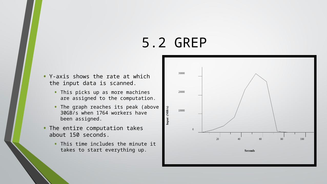
5.2 GREP

• Y-axis shows the rate at which the input data is scanned.

• This picks up as more machines are assigned to the computation.

• The graph reaches its peak (above 30GB/s when 1764 workers have been assigned.

• The entire computation takes about 150 seconds.

• This time includes the minute it takes to start everything up.

5.3 SORT

• The sort program sorts through 10^10 100-byte records.

• This is modeled after the TeraSort benchmark.

• Whole program is less than 50 lines.

• Like Grep the input for the sort program is split up into 64MB pieces.

• The sorted output is partitioned into 4000 files.

• The partitioning function uses the initial bytes of the key to segregate the output into one of the 4000 pieces.

5.3 SORT (Cont.)

• This figure shows the data transfer rate over time for a normal execution of the Sort function.

• The rate peaks at 13GB/s and then starts to die quickly since all of the map tasks get finished before the 200 second mark.

5.3 SORT (Cont.)

• This graph shows the rate of data being sent over the network from the map tasks to the reduce tasks.

• This is started as soon as the first map task finishes

• First bump in the graph is when the first batch of reduce tasks

• This is approximately 1700 reduce tasks, since the entire task was given to around 1700 machines and each machine does one task at a time.

• Then, around 300 seconds into the computation the second batch of reduce tasks finishes so they get shuffled.

• Everything is finished in about 600 seconds.

5.3 SORT (Cont.)

• This figure shows the rate at which sorted data is written to the final output files.

• There is a delay between the last of the first batch of shuffling and the start of the writing since the machines are too busy sorting the intermediate data.

• The writes stay at a more steady rate compared to reading input and shuffling.

• This rate is about 2-4GB/s.

• The writes are finished by around 850 seconds.

• The entire computation takes a total of 891 seconds.

• (this rate is similar to the best reported result by TeraSort [1057 seconds]).

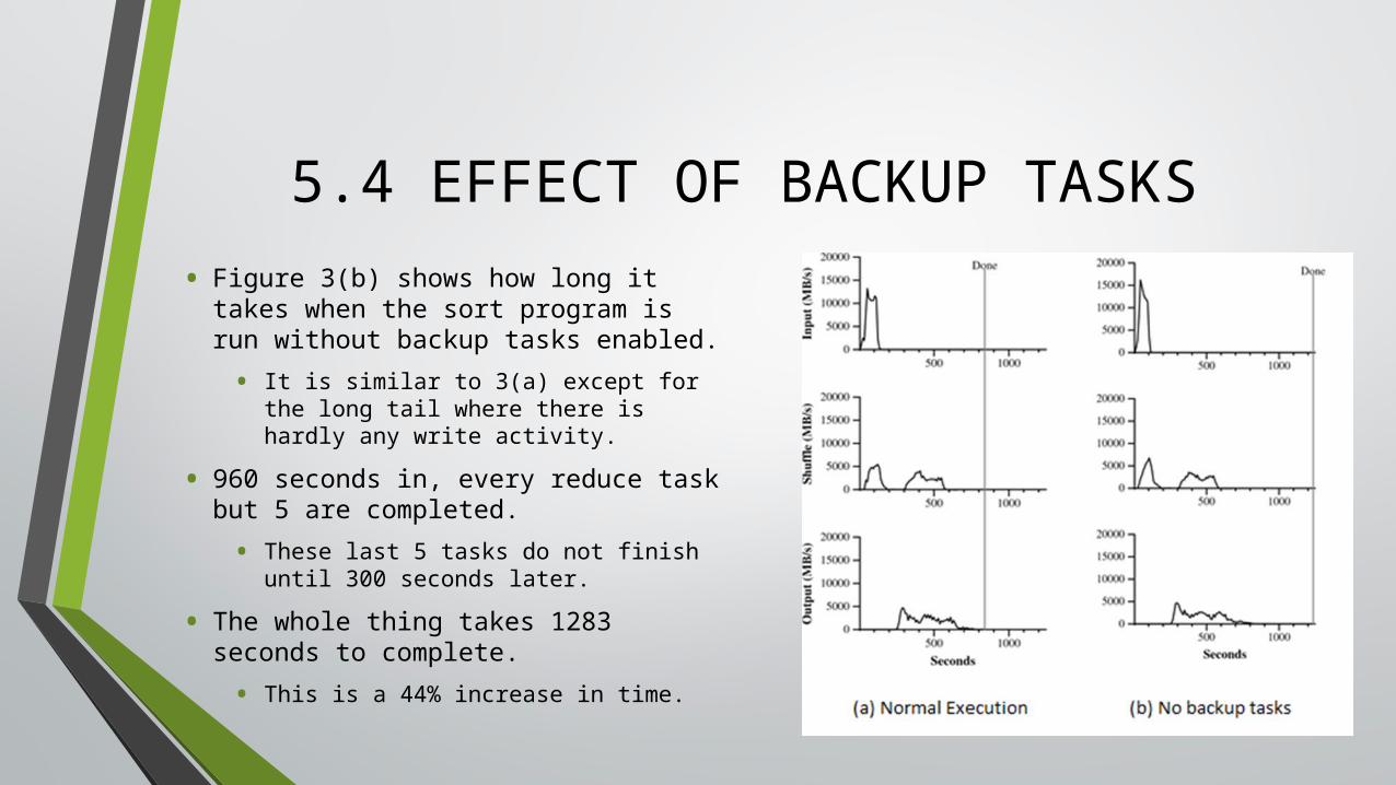
5.4 EFFECT OF BACKUP TASKS• Figure 3(b) shows how long it takes

when the sort program is run without backup tasks enabled.

• It is similar to 3(a) except for the long tail where there is hardly any write activity.

• 960 seconds in, every reduce task but 5 are completed.

• These last 5 tasks do not finish until 300 seconds later.

• The whole thing takes 1283 seconds to complete.

• This is a 44% increase in time.

5.5 MACHINE FAILURES• Figure 3(c) shows the sort program executing where they

intentionally killed 200 of the 1746 workers several minutes into the operation.

• Since the machines were still functioning, the underlying cluster scheduler immediately restarted new worker processes on the “killed” machines.

• The graph shows negative input, this is when the machines were killed.

• The input goes into the negatives because the data was lost, and needed to be redone.

• The whole thing is finished after 933 seconds

• This is only a 5% increase in time over the normal execution.

6. EXPERIENCE

• Extraction of data for popular queries

• Google Zeitgeist

• Extracting properties of web pages

• Geographical locations of web pages for localized search

• Clustering problems for Google News and Shopping

• Large-scale machine learning problems and graph computations

6.1 LARGE SCALE INDEXING

• Production Indexing System

• Produces data structures for searches

• Completely rewritten with MapReduce

• What it does:

• Crawler gathers approx. 20 TB of documents

• Indexing Process: 5-10 map reduce operations

6.1 LARGE SCALE INDEXING (Cont.)• Indexing code is Simpler

• 3800 lines of C++ to 700 w/ MapReduce

• Improved Performance

• Separates unrelated computations

• Avoids extra passes over data

• Easier to Operate

• MapReduce handles issues without operator intervention

• Machine failures, slow machines, networking hiccups

7. RELATED WORK

• MapReduce can be viewed as a simplification of many system’s programming models to be adaptable and scalable

• Works off the restricted model of pushing data to be stored locally on the worker’s system

• Backup system similar to Charlotte System with the fix of the ability to skip bad records caused by failures

8. CONCLUSION

• Been successfully used at Google for different purposes

• Easy for programmers to use, even without the background of distributed and parallel systems

• Used well to sorting, data mining, machine learning and many more

• BIGGEST LESSON: Network bandwidth is a scarce resource, doing storage and calculations locally saves this resource

APPX. A: ”A WORD FREQUENCY”

• Code is divided into three functions• main

• WordCounter

• Adder

• WordCounter is used for the Map function

• Skips any leading whitespace and then parses words out of text

• The word itself is the key, the value is 1

• Adder is used for the Reduce function

• Iterates through keys, and adds the values of the same key together

• Since the value is 1, this has the effect of incrementing a counter for the number of times a word is used

APPX. A: ”A WORD FREQUENCY”

Image taken from OSDI ‘04 Presentation by Jeff Dean and Sanjay Ghemawat.