Mapping Chemical Contaminants in Oceanic Sediments Around Point

Loma’s Treated Wastewater OutfallKerry Ritter

Ken Schiff

N. Scott Urquhart

Dawn Olson

Ami Groce

Tim Stebbins

Overview

Motivation Problems with current methods Kriging offers a more sophisticated statistical

alternative Provides predictions as well as prediction

errors Allows for a cost-efficiency analyses for any

sampling density or configuration

Maps are useful tools for understanding and managing resources

Spatial patterns are recognized more easily with visual displays

Can quickly locate disturbance, assess its relative magnitude and extent, and weigh risk to neighboring areas

Maps are effective and efficient media for communicating information to the public

How do we design the “optimal” sampling grid?

• Depends on goals of the study

• Samples closer together tend to be more alike than samples farther apart

• Placing samples to far apart may make extrapolation to non-sampled locations suspect

• Placing samples too close together may be redundant and waste resources

Current maps

Often based on sparse data (< 30 sites) Use simple interpolation methods

– Spline smoothing– Triangulation– Linear interpolation

Do not provide measures of uncertainty Cannot determine how dense a sampling grid

is optimal

Core Grid Core Grid + Phase I

What is kriging?

A statistical tool used to create maps Predictions = weighted average of neighbors Weights based on the strength of spatial

correlation Provides estimate of confidence Optimal Available in many mapping or statistical

software packages

Kriging Predictions (Core + Phase I)

Kriging Errors(Core + Phase I)

For kriging understanding the spatial variablity is key

Determines weighting factors for kriging

Provides estimates of kriging errors– Confidence intervals– Cost-efficiency analyses for future studies

How do we model spatial variability?

Variogram= variance of paired sample differences as a function of distance between pairs

Measure of spatial correlation Apply statistical models for fitting variogram

– Spherical– Gaussian– Exponential– Linear

Use method of least squares to fit parameters

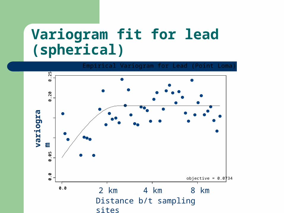
Empirical Variogram for Lead (Point Loma)

Log transformed and detrendeddistance

ga

mm

a

0.0 0.02 0.04 0.06

0.0

0.0

50

.10

0.1

50

.20

0.2

5

distance

ga

mm

a

0.0 0.02 0.04 0.06

0.0

0.0

50

.10

0.1

50

.20

0.2

5

objective = 0.0734

2 km 8 km4 km

variogram

Distance b/t sampling sites

Variogram fit for lead (spherical)

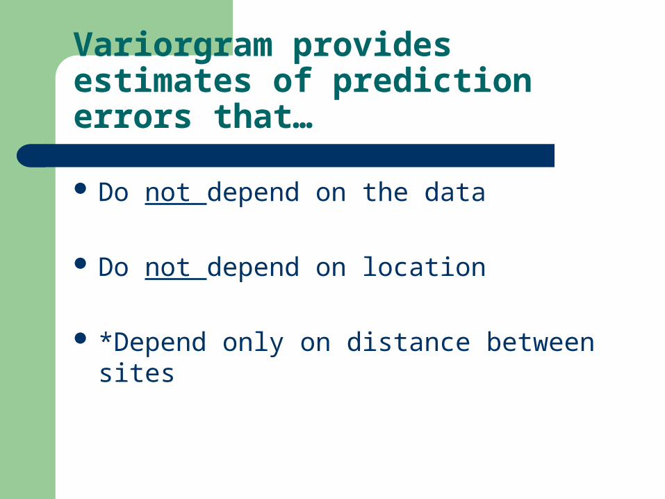
Variorgram provides estimates of prediction errors that…

Do not depend on the data

Do not depend on location

*Depend only on distance between sites

Link variogram to cost efficiency

Can determine prediction error for any grid spacing/configuration

Can weigh the cost of increasing sampling effort with benefit of precision

Percent error v. density

1 2 3 4 5

60

70

80

90

10

0

Core 4km 2.5km 1km 0.5km

Per

cent

Cor

e E

rror

Sampling density

Kriging Predictions (Core + Phase I)

Kriging Errors(Core + Phase I)

Summary

Kriging offers a more sophisticated statistical alternative for creating maps

Provides predictions as well as prediction errors Errors are independent of data, but depend only on

distance between sampling sites Modeling the variogram is key Allows for a cost-efficiency analyses for any sampling

density or configuration– Uneven allocation of resources, targeted sampling