
Manolescu's Seiberg-Witten Floer homotopy type · 2015-08-19 · Manolescu’s Seiberg-Witten Floer...
27
Seiberg-Witten Floer homotopy type Manolescu’s Seiberg-Witten Floer homotopy type Nobuhiro Nakamura The University of Tokyo September 13, 2007 Seiberg-Witten Floer homotopy type Introduction Seiberg-Witten Floer stable homotopy types Seiberg-Witten trajectories Finite dimensional approximation The Conley index Construction of the invariant Relative Bauer-Furuta invariants Gluing formula for relative BF invariants S-duality for Conley indices Gluing formula Cobordism Applications
Transcript of Manolescu's Seiberg-Witten Floer homotopy type · 2015-08-19 · Manolescu’s Seiberg-Witten Floer...

Seiberg-Witten Floer homotopy type
Manolescu’s Seiberg-Witten Floer homotopy type
Nobuhiro Nakamura
The University of Tokyo
September 13, 2007
Seiberg-Witten Floer homotopy type
Introduction
Seiberg-Witten Floer stable homotopy typesSeiberg-Witten trajectoriesFinite dimensional approximationThe Conley indexConstruction of the invariant
Relative Bauer-Furuta invariants
Gluing formula for relative BF invariantsS-duality for Conley indicesGluing formulaCobordism
Applications
Seiberg-Witten Floer homotopy type
Introduction
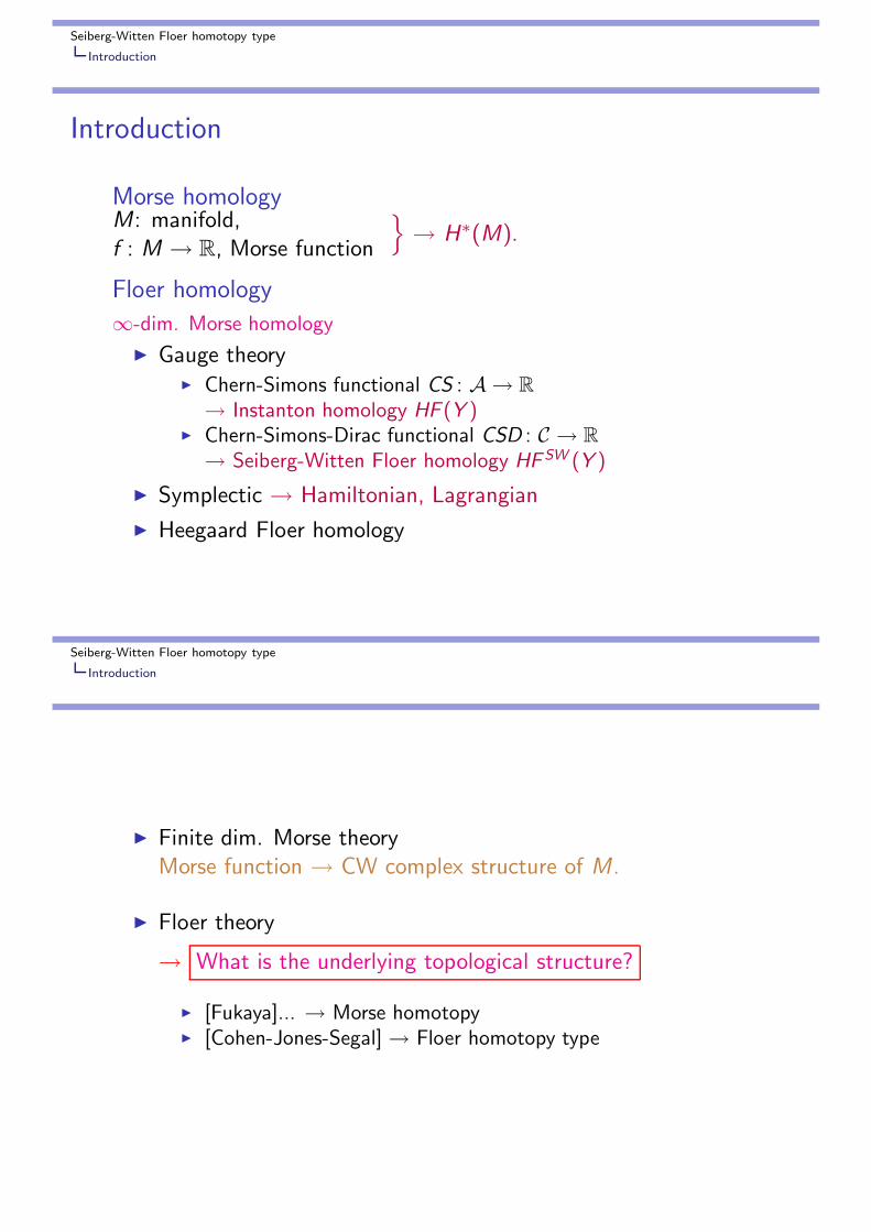
Introduction
Morse homologyM: manifold,f : M → R, Morse function
→ H∗(M).
Floer homology
∞-dim. Morse homology
Gauge theory Chern-Simons functional CS : A → R
→ Instanton homology HF (Y ) Chern-Simons-Dirac functional CSD : C → R
→ Seiberg-Witten Floer homology HF SW (Y )
Symplectic → Hamiltonian, Lagrangian
Heegaard Floer homology
Seiberg-Witten Floer homotopy type
Introduction
Finite dim. Morse theoryMorse function → CW complex structure of M.
Floer theory
→ What is the underlying topological structure?
[Fukaya]... → Morse homotopy [Cohen-Jones-Segal] → Floer homotopy type

Seiberg-Witten Floer homotopy type
Introduction
[Manolescu]
In the Seiberg-Witten Floer case, (Y : 3-manifold with b1 = 0 or 1,)
it is defined a pointed S1-space (prespectrum) SWF (Y ) s.t.
H∗(SWF (Y )) ∼= HF SW∗ (Y ).
Idea- Gauge group = U(1).
- The compactness of the moduli.
→Finite dimensional
approximation
→ The Conley index
Cf. [Frauenfelder ’04] → Moment Floer homology.
[Cohen ’07] →Hamiltonian Floer homology ofthe cotangent bundle
Seiberg-Witten Floer homotopy type
Introduction
References
1. [Manolescu1]Seiberg-Witten-Floer stable homotopy type of three-manifoldswith b1 = 0,
Geom. Topol. 7 (2003) 889–932.
2. [Manolescu2]A gluing formula for the relative Bauer-Furuta invariants,
J. Diff. Geom. 76 (2007) 117–153.
3. [Kronheimer-Manolescu]Periodic Floer pro-spectra for the Seiberg-Witten equations,
preprint, arXive math/0203243.

Seiberg-Witten Floer homotopy type
Introduction
Contents
Definition of Seiberg-Witten Floer stable homotopy types
Relative Bauer-Furuta invariants
Gluing formula for relative BF invariants.
Applications
Seiberg-Witten Floer homotopy type
Seiberg-Witten Floer stable homotopy types
Seiberg-Witten Floer stable homotopy types
Seiberg-Witten trajectories
Finite dimensional approximations
The Conley index
Construction of the invariants

Seiberg-Witten Floer homotopy type
Seiberg-Witten Floer stable homotopy types
Seiberg-Witten trajectories
Seiberg-Witten trajectories
Y : oriented closed 3-manifold, g : metric.
c : Spinc -structure.→ W0: the spinor bundle, L = det W0.
If b1 = 0, ⇒ ∃ flat connection A0 on L unique up to gauge.→ ∂0 : Γ(W0)→ Γ(W0), Dirac operator.
A(L) := U(1)-connections on L = A0 + iΩ1(Y ).
For A = A0 + a
→ ∂a = ρ(a) + ∂0, the Dirac op. associated to A,where ρ(a) is the Clifford multiplication.
Seiberg-Witten Floer homotopy type
Seiberg-Witten Floer stable homotopy types
Seiberg-Witten trajectories
G = Map(Y ,S1) y C := iΩ1(Y )⊕ Γ(W0) by
u(a, φ) = (a − 2u−1du, uφ).
Fix k ≥ 4.G ← L2
k+2-completionC ← L2
k+1-completion
Chern-Simons-Dirac functional, CSD : C → R ,
CSD(a, φ) =1
2
(
−
∫
Y
a ∧ da +
∫
Y
〈φ, ∂aφ〉d vol
)
.
If b1 = 0 ⇒ CSD is G-invariant.
CSD(u(a, φ)) = CSD(a, φ).
Seiberg-Witten Floer homotopy type
Seiberg-Witten Floer stable homotopy types
Seiberg-Witten trajectories
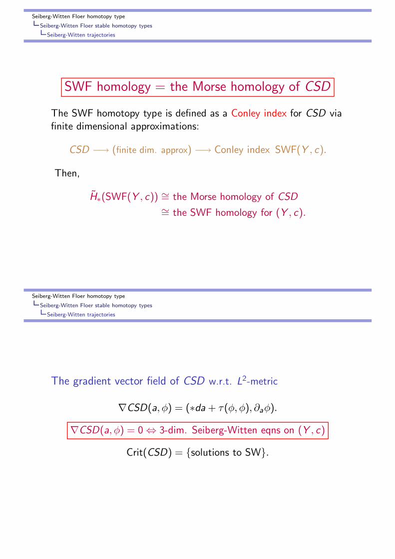
SWF homology = the Morse homology of CSD
The SWF homotopy type is defined as a Conley index for CSD viafinite dimensional approximations:
CSD −→ (finite dim. approx) −→ Conley index SWF(Y , c).
Then,
H∗(SWF(Y , c)) ∼= the Morse homology of CSD
∼= the SWF homology for (Y , c).
Seiberg-Witten Floer homotopy type
Seiberg-Witten Floer stable homotopy types
Seiberg-Witten trajectories
The gradient vector field of CSD w.r.t. L2-metric
∇CSD(a, φ) = (∗da + τ(φ, φ), ∂aφ).
∇CSD(a, φ) = 0⇔ 3-dim. Seiberg-Witten eqns on (Y , c)
Crit(CSD) = solutions to SW.
Seiberg-Witten Floer homotopy type
Seiberg-Witten Floer stable homotopy types
Seiberg-Witten trajectories
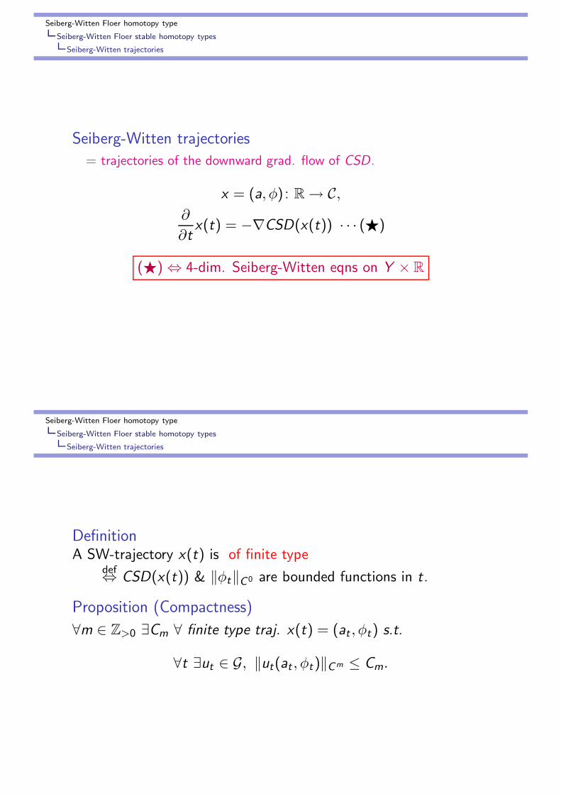
Seiberg-Witten trajectories
= trajectories of the downward grad. flow of CSD.
x = (a, φ) : R→ C,
∂
∂tx(t) = −∇CSD(x(t)) · · · (⋆)
(⋆)⇔ 4-dim. Seiberg-Witten eqns on Y × R
Seiberg-Witten Floer homotopy type
Seiberg-Witten Floer stable homotopy types
Seiberg-Witten trajectories
DefinitionA SW-trajectory x(t) is of finite type
def⇔ CSD(x(t)) & ‖φt‖C0 are bounded functions in t.
Proposition (Compactness)
∀m ∈ Z>0 ∃Cm ∀ finite type traj. x(t) = (at , φt) s.t.
∀t ∃ut ∈ G, ‖ut(at , φt)‖Cm ≤ Cm.

Seiberg-Witten Floer homotopy type
Seiberg-Witten Floer stable homotopy types
Seiberg-Witten trajectories
Projection to the Coulomb gauge
CSD is G-invariant ⇒ Want to consider CSD/G : C/G → R.
Instead of dividing by G, project to the slice at (0, 0).
G0 :=
u = e iξ
∣∣∣∣ξ : Y → R,
∫
Y
ξ = 0
,
G0 y C free,
G/G0 = S1 ← the stabilizer of (0, 0).
- V := i ker d∗ ⊕ Γ(W0). ← The slice at (0, 0)
⇒ ∀(a, φ) ∈ C,∃1u ∈ G0, u(a, φ) ∈ V .
This gives the Coulomb projection Π: C → V .
Seiberg-Witten Floer homotopy type
Seiberg-Witten Floer stable homotopy types
Seiberg-Witten trajectories
Choose a metric g on V s.t.
Π′ ∇L2(CSD) = ∇g (CSD|V ),
where Π′ = the differential of Π. Then,
Π-projection of ∇L2(CSD) trajectory↔ Traj. of ∇g (CSD|V ).
- Note ∇g (CSD|V ) is S1-equivariant.
Decompose ∇g (CSD|V ) as ∇g (CSD|V ) = l + c , where l : linear, l(a, φ) = (∗da, ∂0φ), c : quadratic, compact.
We concentrate on trajectories
x : R→ V ,∂
∂tx(t) = −(l + c)(x(t)).
Seiberg-Witten Floer homotopy type
Seiberg-Witten Floer stable homotopy types
Finite dimensional approximation
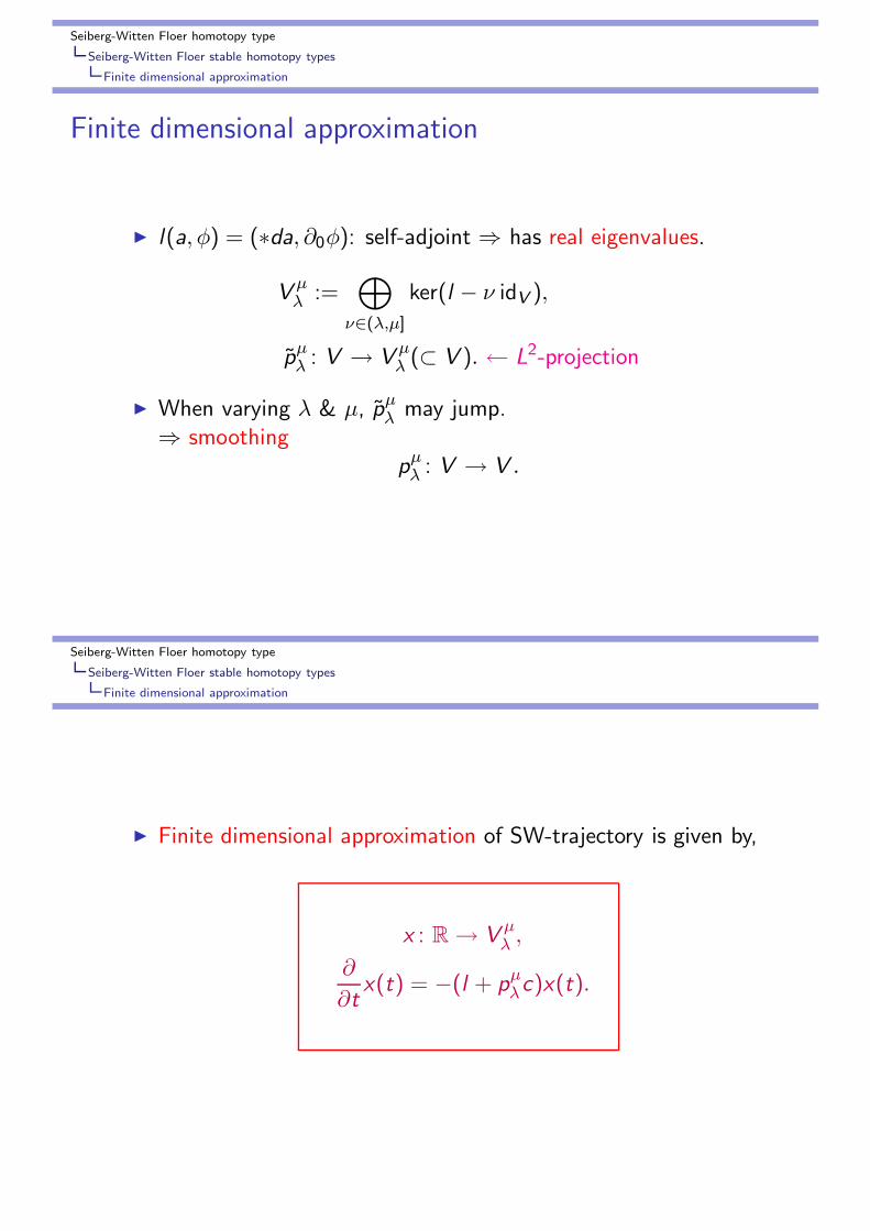
Finite dimensional approximation
l(a, φ) = (∗da, ∂0φ): self-adjoint ⇒ has real eigenvalues.
Vµλ :=
⊕
ν∈(λ,µ]
ker(l − ν idV ),
pµλ : V → V
µλ (⊂ V ). ← L2-projection
When varying λ & µ, pµλ may jump.
⇒ smoothingp
µλ : V → V .
Seiberg-Witten Floer homotopy type
Seiberg-Witten Floer stable homotopy types
Finite dimensional approximation
Finite dimensional approximation of SW-trajectory is given by,
x : R→ Vµλ ,
∂
∂tx(t) = −(l + p
µλc)x(t).

Seiberg-Witten Floer homotopy type
Seiberg-Witten Floer stable homotopy types
Finite dimensional approximation
By Compactness Proposition,
∃R ≫ 1, s.t. (∀ finite type traj. of l + c) ⊂ B(R),
where B(R) is the open ball in L2k+1(V ) with radius R centered at 0.
Fix such an R .
Proposition
For sufficient large −λ & µ,
x(t): a trajectory of l + pµλc,
∀t, x(t) ∈ B(2R)⇒ ∀t, x(t) ∈ B(R).
Next, Gradient flows of l + pµλc ⇒ Conley index.
Seiberg-Witten Floer homotopy type
Seiberg-Witten Floer stable homotopy types
The Conley index
The Conley index
M: finite dim. manifold
ϕ : M × R→ M, a continuous flow,
ϕ0 = id,
ϕs+t =ϕs ϕt .
S(⊂ M) is invariantdef⇔ ∀t ϕt(S) = S .
For A(⊂ M), the invariant set of A is,
Inv(A) :=⋂
t
ϕt(A) = x ∈ A | ∀t ϕt(x) ∈ A.

Seiberg-Witten Floer homotopy type
Seiberg-Witten Floer stable homotopy types
The Conley index
A compact subset S(⊂ M) is an isolated invariant set if
∃ cpt set A s.t. S = Inv(A) ⊂ Int(A).
A is called an isolating neighborhood.
Seiberg-Witten Floer homotopy type
Seiberg-Witten Floer stable homotopy types
The Conley index
DefinitionA pair of compact sets (N,L), L ⊂ N ⊂ M, is an index pair for aninv. set S if
1. S = Inv(N \ L) ⊂ Int(N \ L).
2. L is an exit set:∀x ∈ N, ∀t > 0 s.t. ϕt(x) 6∈ N ⇒ ∃τ ∈ [0, t) ϕτ (x) ∈ L.
3. L is positively invariant:x ∈ L, t > 0, ϕ[0,t](x) ⊂ N ⇒ ϕ[0,t](x) ⊂ L.

Seiberg-Witten Floer homotopy type
Seiberg-Witten Floer stable homotopy types
The Conley index
An example of index pair
Seiberg-Witten Floer homotopy type
Seiberg-Witten Floer stable homotopy types
The Conley index
Theorem (Conley)
For every iso. inv. set S & isolating nbd. A,
∃ index pair (N,L) for S s.t. N ⊂ A.
DefinitionThe Conley index of S is,
I (ϕ,S) := the pointed homotopy type of (N/L, [L]).

Seiberg-Witten Floer homotopy type
Seiberg-Witten Floer stable homotopy types
The Conley index
Properties
I (ϕ,S) is independent of the choice of (N,L).
(Continuation)ϕλ (λ ∈ [0, 1]): continuous family of flows.Sλ: invariant sets for ϕλ.If ∀λ A is an isolating nbd. of Sλ, i.e., Inv(A) = Sλ,
⇒ I (ϕ0,S0) ∼= I (ϕ1,S1).
Seiberg-Witten Floer homotopy type
Seiberg-Witten Floer stable homotopy types
The Conley index
Examples
1. I (ϕ, ∅) = 1pt
2. If p is a crit. point of a grad. flow with index=k,
I (ϕ, p) ∼= Sk .
←→

Seiberg-Witten Floer homotopy type
Seiberg-Witten Floer stable homotopy types
The Conley index
3. M: closed,f : M → R, Morse function s.t. Morse-Smale,S := Crit. points of f & trajectories between them
⇒ H∗(I (ϕ,S)) ∼= the Morse homology of f .
Seiberg-Witten Floer homotopy type
Seiberg-Witten Floer stable homotopy types
The Conley index
Theorem (Floer et al.)
G: a compact Lie group,
G y M preserving ϕt ,
S: a G-invariant iso. inv. set.
Then, the G-equivariant Conley index IG (ϕ,S) is defined as a
pointed G-homotopy type.

Seiberg-Witten Floer homotopy type
Seiberg-Witten Floer stable homotopy types
Construction of the invariant
Construction of the invariant
Finite dim. approx. x : R→ Vµλ is “stable” when −λ & µ→∞.
⇒ The Conley index is also stable.
⇒ SWF(Y , c) is defined as an object in a certain stablehomotopy category.
Let S1 act on R & C as:
S1 y R: trivially
S1 y C: by multiplication.
Seiberg-Witten Floer homotopy type
Seiberg-Witten Floer stable homotopy types
Construction of the invariant
DefinitionC is S1-equivariant graded suspension category as follows:
Object: (X ,m, n)X : pointed S1-space, m ∈ Z, n ∈ Q.
Morphism:
(X ,m, n), (X ′,m′, n′)S1 =
∅ if n− n′ 6∈ Z,
colimk,l
[
(Rk ⊕ Cl)+ ∧ X , (Rk+m−m′
⊕ Cl+n−n′)+ ∧ X ′]
S1,
if n − n′ ∈ Z.
Note: (X ,m, n) ∼= (R+ ∧ X ,m + 1, n) ∼= (C+ ∧ X ,m, n + 1).
(X ,m, n) 7→ (X ,m − 1, n) ∼= (R+ ∧ X ,m, n)(X ,m, n) 7→ (X ,m, n − 1) ∼= (C+ ∧ X ,m, n)

Seiberg-Witten Floer homotopy type
Seiberg-Witten Floer stable homotopy types
Construction of the invariant
m 7→ m + 1 ↔ (formal) desuspension by R+
n 7→ n + 1 ↔ (formal) desuspension by C+
Denote (X , 0, 0) by X .
For a finite dim. vector space E with trivial S1-action,
Σ−EX := (E+ ∧ X , 2 dimR E , 0).
For a finite dim. vector space E with free S1-action except 0,
Σ−EX := (X , 0, dimC E ).
Seiberg-Witten Floer homotopy type
Seiberg-Witten Floer stable homotopy types
Construction of the invariant
Recall our situation.
x : R→ Vµλ ,
∂
∂tx(t) = −(l + p
µλc)x(t),
−→ gradient flow ϕλ
µ.
Define the isolated invariant set Sµλ by
Sµλ := Inv(V µ
λ ∩ B(2R))
=Crit. points in B(R) & trajectories connecting them
−→ Iµλ = IS1(ϕλ
µ,Sµλ ).

Seiberg-Witten Floer homotopy type
Seiberg-Witten Floer stable homotopy types
Construction of the invariant
Definition
SWF(Y , c) :=(
Σ−V 0λ I
µλ , 0, n(Y , c , g)
)
,
where n(Y , c , g) is a rational number determined from eta invariants ofDirac & sign.
Seiberg-Witten Floer homotopy type
Seiberg-Witten Floer stable homotopy types
Construction of the invariant
Why Σ−V 0λ I
µλ & what is n(Y , c, g)?
Morse index of the reducible (0, 0) = #negative eigenvalues
= dimV 0λ .← depending on λ, g
⇒ Σ−V 0λ I
µλ
gt : path of metric g0gt∼ g1.
If λ is not eigenvalue for ∀gt ,
⇒ dim(V 0λ )g1 − dim(V 0
λ )g0 =SF ((∂)gt )
=n(Y , c , g1)− n(Y , c , g0).
⇒ Σ−V 0λ−Cn(Y ,c,g)
Iµλ

Seiberg-Witten Floer homotopy type
Seiberg-Witten Floer stable homotopy types
Construction of the invariant
TheoremSWF(Y , c) = Σ−V 0
λ−Cn(Y ,c,g)
Iµλ is independent of parameters.
Example
If Y admits a metric of positive scaler curvature
⇒ The reducible θ is the unique solution.
⇒ Sµλ = θ. ⇒ I
µλ = (V 0
λ )+.
⇒ SWF(Y , c) =(
C−n(Y ,c,g))+
.
Y = S3 ⇒ SWF(Y ) = S0.
Y = Poincare sphere ⇒ SWF(Y ) = C+.
Seiberg-Witten Floer homotopy type
Relative Bauer-Furuta invariants
Relative Bauer-Furuta invariants
First, we recall ordinary Bauer-Furuta invariants.
Bauer-Furuta invariantsBauer-Furuta invariant is a stable cohomotopy refinement of theSeiberg-Witten invariant defined by [Bauer-Furuta].
X : closed ori. 4-mfd. For simplicity, suppose b1 = 0.
c : Spinc -structure on X .
Fix a connection A0 on the determinant line bundle det c of c .

Seiberg-Witten Floer homotopy type
Relative Bauer-Furuta invariants
Monopole map
SW : i ker d∗(⊂ iΩ1(X ))⊕ Γ(W +)→iΩ+(X )⊕ Γ(W−)
(a, φ) 7→(F+
A0+a+ σ(φ, φ∗),D
A0+aφ)
Decompose SW asSW = L + C ,
where L: linear & C : quadratic, compact.
Take a finite dim. approx. of L + C :
L + pνC : U ′ → U.
The Bauer-Furuta invariant BFX (c) is defined as
BFX (c) = [L + pνC ] ∈
(
CindC D
A0
)+,(
Rb+)+
S1
.
Seiberg-Witten Floer homotopy type
Relative Bauer-Furuta invariants
Relative Bauer-Furuta invariants
Y : closed ori. 3-manifold, b1(Y ) = 0.
X : compact ori. 4-manifold, ∂X = Y .For simplicity, b1(X ) = 0.
Fix a metric g as in the picture below.
c : Spinc -structure on X . → c := c |Y , a Spinc -str. on Y.
Fix a connection A0 on det c s.t. A0 := A0|Y is a flat conn.on det c .
X =
Seiberg-Witten Floer homotopy type
Relative Bauer-Furuta invariants
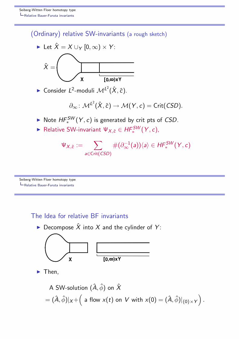
(Ordinary) relative SW-invariants (a rough sketch)
Let X = X ∪Y [0,∞) × Y :
X =
Consider L2-moduliML2(X , c).
∂∞ : ML2(X , c)→M(Y , c) = Crit(CSD).
Note HF SW∗ (Y , c) is generated by crit pts of CSD.
Relative SW-invariant ΨX ,c ∈ HF SW∗ (Y , c),
ΨX ,c :=∑
a∈Crit(CSD)
#(∂−1∞ (a))〈a〉 ∈ HF SW
∗ (Y , c)
Seiberg-Witten Floer homotopy type
Relative Bauer-Furuta invariants
The Idea for relative BF invariants
Decompose X into X and the cylinder of Y :
Then,
A SW-solution (A, φ) on X
= (A, φ)|X+(
a flow x(t) on V with x(0) = (A, φ)|0×Y
)
.

Seiberg-Witten Floer homotopy type
Relative Bauer-Furuta invariants
Monopole map
Ω1g (X ) := a ∈ Ω1(X ) | a ∈ ker d∗, a|∂X (ν) = 0,
where ν: the unit normal vector to the boundary Y .
Fix a large µ.
Monopole map
SW : iΩ1g (X )⊕ Γ(W +)→ iΩ+(X )⊕ Γ(W−)⊕ V
µ−∞,
SW (a, φ) = (FA0+a
+ σ(φ, φ),DA0+a
φ, pµΠi∗(a, φ)),
where i∗ : the restriction to ∂X = Y ,
Π : the Coulomb projection to V ,
pµ : V → Vµ−∞, the L2-projection.
Write briefly as SW : CX → U ⊕ Vµ−∞.
Seiberg-Witten Floer homotopy type
Relative Bauer-Furuta invariants
Decompose SW : CX → U ⊕ Vµ−∞ as SW = L + C ,
where L: linear & C : quadratic.
Take a finite dimensional subspace U ⊂ U , and fix λ≪ 0.⇒ Put U ′ := L−1(U × V
µλ ), and
SWU := L + prU×Vµλ
C : U ′ → U × Vµλ .
Fix small ε > 0. Let B(U, ε) ⊂ U be the ε-ball in U.
Mε := SW−1U (B(U, ε)× V
µλ ).← Almost the SW-moduli

Seiberg-Witten Floer homotopy type
Relative Bauer-Furuta invariants
Fix R ′ ≫ 1.Let B(U ′,R ′) ⊂ U ′ be the R ′-ball.S(U ′,R ′) = ∂B(U ′,R ′).
M ′ :=Mε ∩ B(U ′,R ′),
K ′ :=Mε ∩ S(U ′,R ′),
M := prV µλi∗(M ′),
K := prV µλi∗(K ′).
⇒Can find an index pair (N,L)s.t. M ⊂ N, K ⊂ L.
y prV µ
λi∗
Seiberg-Witten Floer homotopy type
Relative Bauer-Furuta invariants
⇒SWU : B(U ′,R ′)/S(U ′,R ′)→ (B(U, ε)/S(U, ε)) ∧ N/L.
⇒ΨX ,c : (U ′)+ → U+ ∧ Iµλ .
The relative Bauer-Furuta invariant is,
BFX (c) = [ΨX ,c ] ∈(
Sk , b+(X ), n(X , c , g))
,SWF(Y , c)
S1
where k = indAPS DA.

Seiberg-Witten Floer homotopy type
Gluing formula for relative BF invariants
S-duality for Conley indices
Gluing formula for relative BF invariants
S-duality for Conley indices
f : M → R, Morse function of a n-dim. mfd.⇒ Morse flow ϕf .⇒ The Conley index If = I (ϕf ,S).
−f ⇒ the reverse flow ϕ−f .⇒ The Conley index I−f = I (ϕ−f ,S).
Seiberg-Witten Floer homotopy type
Gluing formula for relative BF invariants
S-duality for Conley indices
Theorem (Cornea)
I−f is a Spanier-Whitehead n-dual of If , i.e.,
∃η : If ∧ I−f → Sn, n-duality map s.t.
η∗ : S0, If ∼=→ I−f ,S
n.
Note For α ∈ S0, If , η∗(α) is given as follows:
S0 ∧ I−fα∧id−−−−→ If ∧ I−f
η−−−−→ Sn.
Corollary
SWF(−Y ) is a S-dual of SWF(Y ).
(∵) CSD−Y = −CSDY .

Seiberg-Witten Floer homotopy type
Gluing formula for relative BF invariants
Gluing formula
Gluing formula
X = X1 ∪Y X2.
η : SWF(Y ) ∧ SWF(−Y )→ S0, the duality map.
BFX = [ΨX ] ∈(S0, b+(X ),−d),S0
S1 ,
BFX1= [ΨX1
] ∈(S0, b+(X1),−d1),SWF(Y )
S1 ,
BFX2= [ΨX2
] ∈(S0, b+(X2),−d2),SWF(−Y )
S1 .
⇒ S• ∧ S•ΨX1
∧ΨX2−−−−−−→ SWF(Y ) ∧ SWF(−Y )η
−−−−→ S•.
Theorem (Gluing formula)
ΨX ≃ η (ΨX1∧ΨX2
).
Seiberg-Witten Floer homotopy type
Gluing formula for relative BF invariants
Cobordism
Cobordism
X : a compact 4-manifold, ∂X = (−Y1) ∪ Y2.
ΨX ∈ (S0, b,−d),SWF(−Y1) ∧ SWF(Y2)S1
y
y
S-duality∼=
D(X ) ∈ (SWF(Y1), b,−d),SWF(Y2)S1
A cobordism X gives a morphism D(X ) between SWF’s.
Theorem
Xa: ∂Xa = (−Y1) ∪ Y2 & Xb: ∂Xb = (−Y2) ∪ Y3.
X = Xa ∪Y2Xb.
⇒ D(X ) = Σb+(Xa),−d(Xa)D(Xb) D(Xa)

Seiberg-Witten Floer homotopy type
Applications
Applicationsto negative definite manifolds
Theorem A (Donaldson)
X: closed ori. 4-mfd with negative definite form ΨX
⇒ ΨX∼= diagonal.
Proof by [Bauer-Furuta]The finite dim approx. of the monopole map:
f : SV := (Rm ⊕Cn+s)+ → (Rm ⊕ Cn)+.
This is S1-equivariant and deg f |(SV )S1 = 1.
LemmaFor f as above, s ≤ 0.
(∵) Use tom Dieck’s character formula.
Seiberg-Witten Floer homotopy type
Applications
Proof of Theorem A.
0 ≥ s = indC D =c2 + b2(X )
8.
∴ ∀c : characteristic c2 + b2(X ) ≤ 0.⇒
[Elkies]Diagonal.

Seiberg-Witten Floer homotopy type
Applications
QuestionDoes an analogue of Theorem A for 4-mfd with boundary?
→ Yes.
Theorem (Froyshov)
X: compact ori. 4-mfd, ∂X = the Poincare 3-sphere.
If ΨX∼= m(−1)⊕ J, where J:negative definite even,
⇒ J = 0 or J = −E8.
Froyshov proved this by the invariant he defined.
This can be proved by using SWF.
Seiberg-Witten Floer homotopy type
Applications
X : negative definite, ∂X = Y . The monopole map f satisfies
[f ] ∈ (Cs)+,SWF(Y , c)S1 & deg f S1= 1.
s(Y , c) := max
(
s
∣∣∣∣∣∃f s.t.
[f ] ∈ (Cs)+,SWF(Y , c)S1
degf S1= 1
)
.
Recall, if Y is the Poincare 3-sphere ⇒ SWF(Y ) = C+.
Then, s(Y ) = 1 .
∵ f ∈ (Cs)+, C+S1 & deg f S1= 1 ⇒ s − 1 ≤ 0.
Seiberg-Witten Floer homotopy type
Applications
TheoremX: compact ori. negative definite, ∂X = Y .
For ∀ characteristic c
b2(X ) + c2
8≤ s(Y , c),
Proof.The monopole map f for c satisfies
[f ] ∈ (Ck)+,SWF(Y , c)S1 & deg f S1= 1,
where k = (c2 + b2)/8.Therefore k ≤ s(Y , c).
Seiberg-Witten Floer homotopy type
Applications
Theorem (Froyshov)
X: compact ori. 4-mfd, ∂X = the Poincare 3-sphere.
If ΨX∼= m(−1)⊕ J, where J:negative definite even,
⇒ J = 0 or J = −E8.
Proof
Note that c = (
m︷ ︸︸ ︷
1, . . . , 1, 0, . . . , 0) is a characteristic.⇒ rank J = b2 −m = b2 + c2 ≤ 8s(Y ) = 8.∴ J = 0 or J = −E8.
QuestionWhat is the relation between s(Y ) & Froyshov’s invariants?


![LAGRANGIAN CORRESPONDENCES AND DONALDSON’S TQFT ...math.mit.edu › ~timothyn › papers › sw3.pdf · homology and Seiberg-Witten Floer homology, recently established in [9],](https://static.fdocuments.net/doc/165x107/5f0396ab7e708231d409cb59/lagrangian-correspondences-and-donaldsonas-tqft-mathmitedu-a-timothyn.jpg)


![DONALDSON = SEIBERG-WITTEN FROM MOCHIZUKI · PDF filearxiv:1001.5024v1 [math.dg] 27 jan 2010 donaldson = seiberg-witten from mochizuki’s formula and instanton counting lothar gottsche,](https://static.fdocuments.net/doc/165x107/5a7268f67f8b9aa2538d8f9c/donaldson-seiberg-witten-from-mochizuki-nbsppdf-filearxiv10015024v1.jpg)