MAE 4700/5700 (Fall 2009) Homework 12 Fluid...

MAE 4700/5700 (Fall 2009) Homework 12 Fluid Mechanics

Finite Element Analysis for Mechanical & Aerospace Design of 24

Due Tuesday, November 23nd

, 12:00 midnight

This challenging but very rewarding homework is considering the finite element analysis

of advection-diffusion and incompressible fluid flow problems.

Problem 1 can be addressed by modifying the 1DBVP MatLab programs to

include SUPG stabilization.

Problems 2 and 3 need the FEM libraries provided here that are based on a

stabilized second-order fractional-step method FEM implementation for the

solution of incompressible unsteady Navier-Stokes equations (read the provided

Readme file for the theory, implementation and examples).

Finally, Problem 4 requires that you modify the 2DBVP libraries for scalar fields

(to include time dependence and advection terms) and couple them with the

provided fluid flow libraries in order to address natural convection problems. An

overall algorithm for the needed computational approach is provided.

Problem 1 – Advection-Diffusion problems using SUPG (streamline upwind Petrov-

Galerkin) methods (MatLab)

Consider a one-dimensional stationary diffusion equation:

2

20

d c dcu

dx dx

with boundary conditions as

(0) 0, (1) 1c c

a) Show that by applying classical Galerkin formulation the solution shows wiggles

as long as 2

xPe

, where the Peclet number Pe is defined as u

Pe

. Plot the

computed solution and the exact solution for h=x = 0.1, u = 1 and ε = 0.01.

Repeat the calculation for number of nodes 6, 11 and 21 and 1,0.1,0.005

For each of these cases tabulate the finite element error in max-norm.

b) Modify your 1DBVP and repeat the above calculation by considering an SUPG

formulation. In this case, the weak form is as follows:

1

0e

ek

N

h h h hh h

k

dc dc dw dcu w d p u d

dx dx dx dx

The stabilization parameter is taken as 2

hh

dwhp

dx

where



1coth( ) ,

2

uhElement Peclet Number

Repeat the calculation from case (a) above (h=x=0.1,u=1,=0.01) and show that

the wiggles disappear. Repeat the calculation for number of nodes 6, 11 and 21

and =1, 0.1,0.005 and show the accuracy of the method is now practically O(h2)

for small .

Analytical Solution:

Since the equation is a standard ordinary differential equation, let

𝑐 = 𝑒𝑟𝑥

Thus, the characteristic equation is,

𝑟 −𝜀𝑟 + 𝑢 = 0

And the roots are:

𝑟1 = 0 𝑎𝑛𝑑 𝑟2 =𝑢

𝜀

The general solution now is:

𝑐 = 𝑐1 + 𝑐2𝑒𝑢𝜀𝑥

Applying the boundary conditions and solving for the constants c1 and c2,

𝑐 0 = 𝑐1 + 𝑐2 = 0

𝑐 1 = 𝑐1 + 𝑐2𝑒𝑢𝜀 = 1

𝑐1 = −1

𝑒𝑢𝜀 − 1

, 𝑐2 =1

𝑒𝑢𝜀 − 1

The analytical solution becomes:

𝑐 =𝑒𝑢𝜀𝑥 − 1

𝑒𝑢𝜀 − 1

Derivation of the Weak Form:

From the original equation, multiply by an arbitrary weight function w(x) and integrate

on the domain

𝑢𝑑𝑐

𝑑𝑥𝑤 𝑑𝑥

1

0

− 𝜀𝑑2𝑐

𝑑𝑥2𝑤 𝑑𝑥 = 0

1

0

, ∀𝑤 𝑖𝑛 0 < 𝑥 < 1

Performing integration by parts on the second term,



𝑢𝑑𝑐


1

0

– 𝜀𝑑𝑐

𝑑𝑥𝑤 0

1 + 𝜀𝑑𝑐

𝑑𝑥

𝑑𝑤

𝑑𝑥 𝑑𝑥 = 0

1

0

, ∀𝑤 𝑖𝑛 0 < 𝑥 < 1

Since the displacements at the boundaries are defined, w(0) = w(1) = 0, and we can

simplify the weak form as:

𝑢𝑑𝑐


1

0

+ 𝜀𝑑𝑐

𝑑𝑥

𝑑𝑤

𝑑𝑥 𝑑𝑥 = 0

1

0

, ∀𝑤 𝑖𝑛 0 < 𝑥 < 1

For each element, using the approximations:

𝑤𝑒 = 𝑤𝑒𝑇𝑁𝑒𝑇 , 𝑑𝑤

𝑑𝑥 𝑇

= 𝑤𝑒𝑇𝐵𝑒𝑇

𝑐𝑒 = 𝑁𝑒𝑐𝑒 , 𝑑𝑐

𝑑𝑥 = 𝐵𝑒𝑐𝑒

Substitution into the weak form gives:

𝑤𝑒𝑇 𝐵𝑒𝑇𝜀 𝐵𝑒 𝑑𝑥1

0

𝑐𝑒 + 𝑢𝑁𝑒𝑇𝐵𝑒 𝑑𝑥1

0

𝑐𝑒 = 0

𝑒

Thus, for the MATLAB code modifications,

𝑝 𝑥 = 𝜀, 𝑞 𝑥 = 𝑢, 𝑓 𝑥 = 0

𝐾𝑒 = 𝐵𝑒𝑇𝑝(𝑥) 𝐵𝑒 + 𝑞(𝑥)𝑁𝑒𝑇𝐵𝑒𝑑𝑥1

0

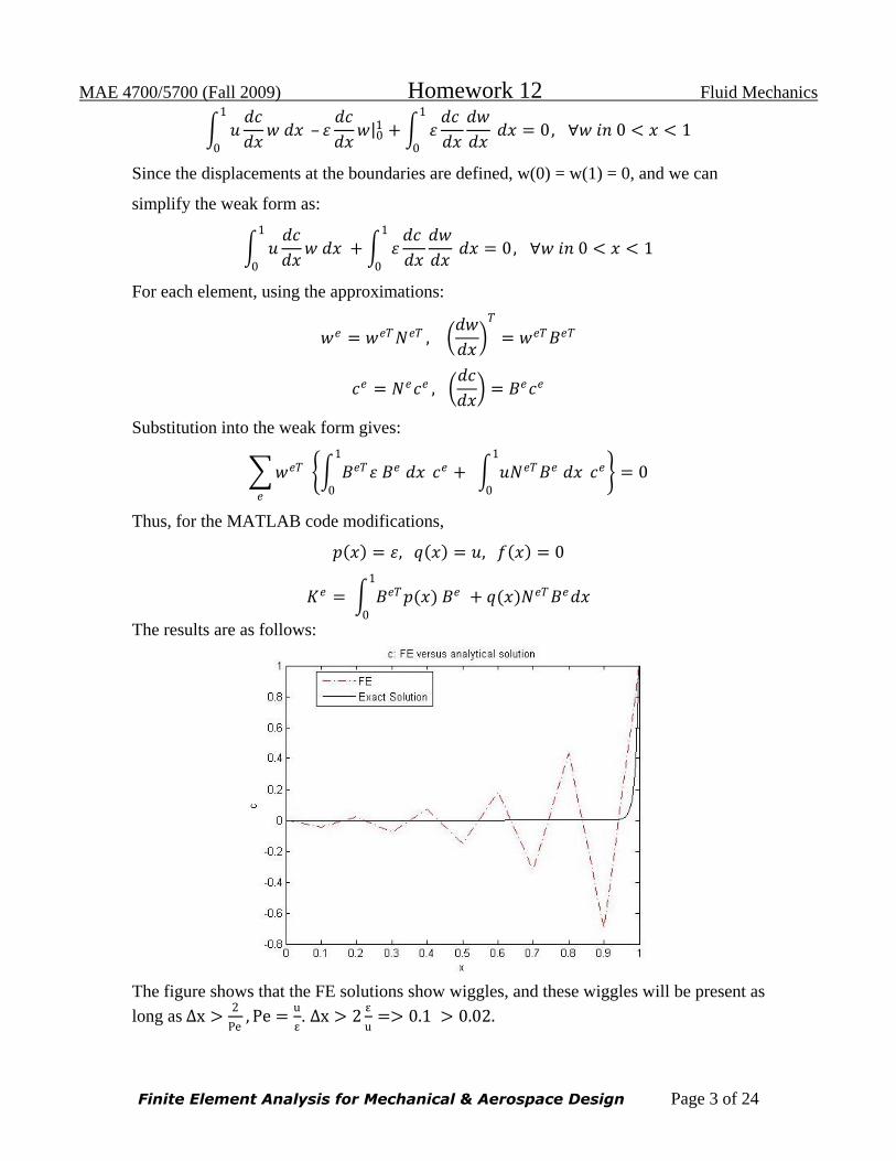
The results are as follows:

The figure shows that the FE solutions show wiggles, and these wiggles will be present as

long as Δx >2

Pe, Pe =

u

ε. Δx > 2

ε

u=> 0.1 > 0.02.



The following figures, however, do not have wiggles because ε is equal to 1 instead of

0.01, which means Δx >2

Pe is not satisfied.

The figure shows that FE solutions approximate the exact solutions very smoothly.

no SUPG (bold - no wiggles & plain - wiggles)

Element size, h ε FE error in max-norm

1/5 1 4.8033E-03

1/5 0.1 1.3338E-01

1/5 0.01 7.0425E-01

1/5 0.005 7.4919E-01

1/10 1 1.2566E-03

1/10 0.1 4.9612E-02

1/10 0.01 5.2073E-01

1/10 0.005 7.3737E-01

1/20 1 3.2167E-04

1/20 0.1 1.5743E-02

1/20 0.01 3.5048E-01

1/20 0.005 5.2684E-01 The above table displays that the finite element errors in maximum norm decrease as the

element size gets smaller and ε increases to 1.

b)

udc

dxw + ε

dc

dx

dw

dx dΩ + pu

dc

dxdΩ = 0

Ωe k

Ne

k=1Ωe

p =hξ

2, ξ = coth α −

1

α & 𝛼 =

uh

2ε



To take the stabilization parameter into account (SUPG), I have modified integrands.m

extensively by adding the following code: B = felm.dN; alpha = qq(felm.x)/(n*2*pp(felm.x));

Ke = Ke + (pp(felm.x)*B'*B + qq(felm.x)*felm.N'*B+... 1/n*qq(felm.x)/2*(coth(alpha)-1/alpha)*B'*B)* felm.detJxW;

fe = fe + ff(felm.x) * felm.N' * felm.detJxW;

The results are as follows:

Unlike previous figures, this figure does not show any wiggles after applying an SUPG

formulation.

The following table also lists finite element errors with SUPG formulation.

SUPG

Element size, h ε FE error in max-norm

1/5 1 4.8686E-03

1/5 0.1 1.6197E-01

1/5 0.01 7.7407E-01

1/5 0.005 7.8846E-01

1/10 1 1.2664E-03

1/10 0.1 5.6909E-02

1/10 0.01 6.6784E-01

1/10 0.005 7.7407E-01

1/20 1 3.2301E-04

1/20 0.1 1.7123E-02

1/20 0.01 4.4247E-01

1/20 0.005 6.6784E-01



This table shows that the finite element errors change relative to the element size for

small ε. With this method, there are no wiggles anymore as shown in figures below.

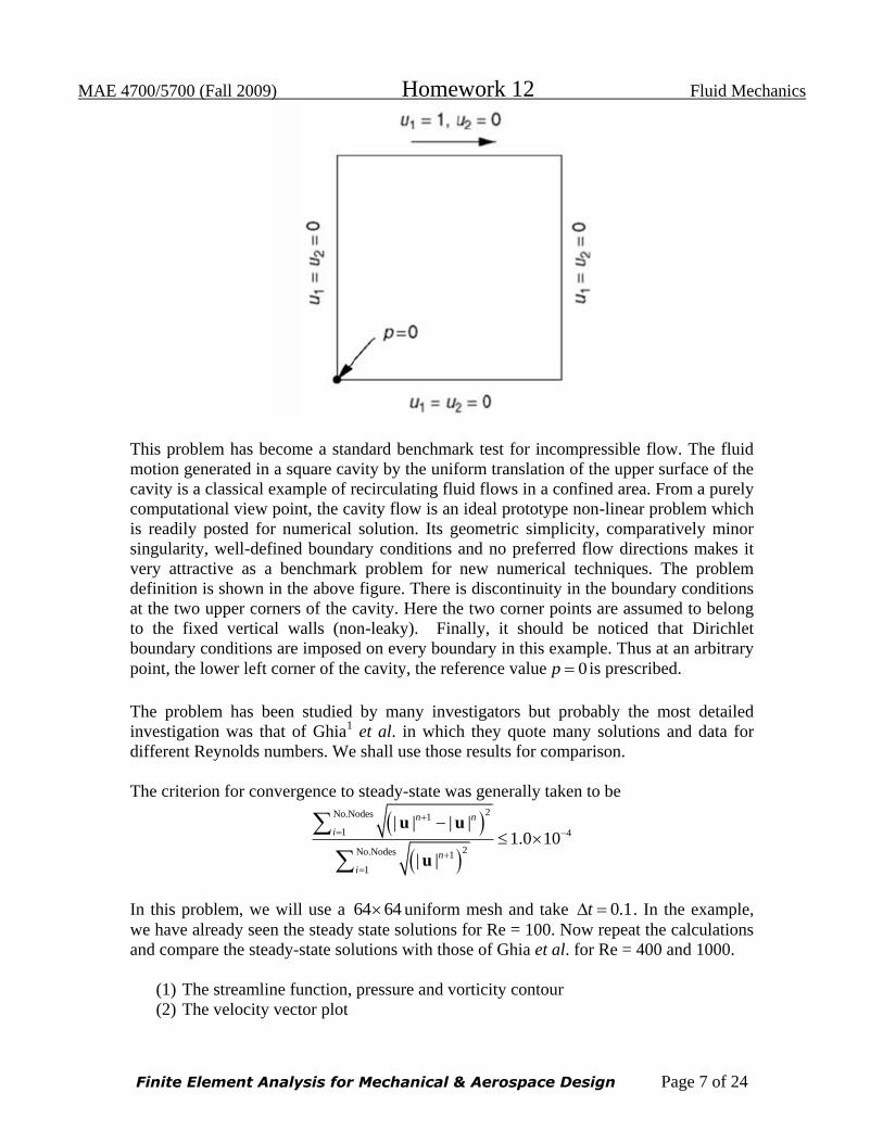
Problem 2 – A lid-driven cavity flow (MatLab)



This problem has become a standard benchmark test for incompressible flow. The fluid

motion generated in a square cavity by the uniform translation of the upper surface of the

cavity is a classical example of recirculating fluid flows in a confined area. From a purely

computational view point, the cavity flow is an ideal prototype non-linear problem which

is readily posted for numerical solution. Its geometric simplicity, comparatively minor

singularity, well-defined boundary conditions and no preferred flow directions makes it

very attractive as a benchmark problem for new numerical techniques. The problem

definition is shown in the above figure. There is discontinuity in the boundary conditions

at the two upper corners of the cavity. Here the two corner points are assumed to belong

to the fixed vertical walls (non-leaky). Finally, it should be noticed that Dirichlet

boundary conditions are imposed on every boundary in this example. Thus at an arbitrary

point, the lower left corner of the cavity, the reference value 0p is prescribed.

The problem has been studied by many investigators but probably the most detailed

investigation was that of Ghia1 et al. in which they quote many solutions and data for

different Reynolds numbers. We shall use those results for comparison.

The criterion for convergence to steady-state was generally taken to be

2No.Nodes 1

1 4

2No.Nodes 1

1

| | | |1.0 10

| |

n n

i

n

i

u u

u

In this problem, we will use a 64 64 uniform mesh and take 0.1t . In the example,

we have already seen the steady state solutions for Re = 100. Now repeat the calculations

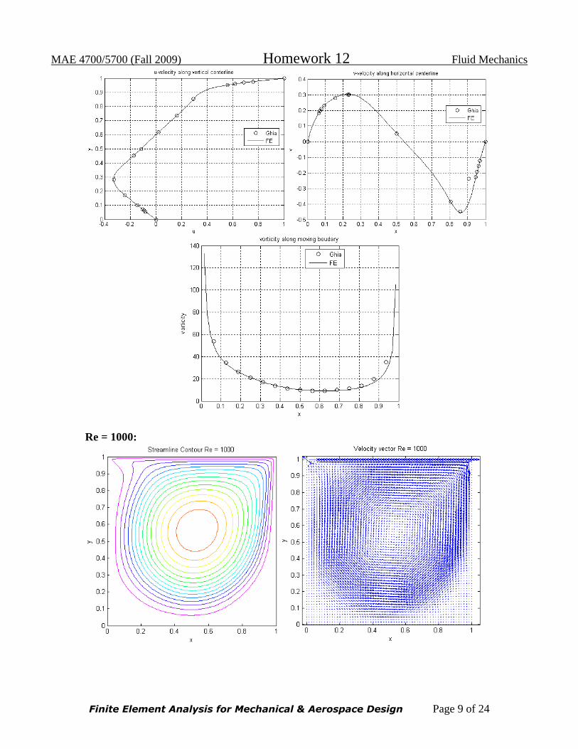
and compare the steady-state solutions with those of Ghia et al. for Re = 400 and 1000.

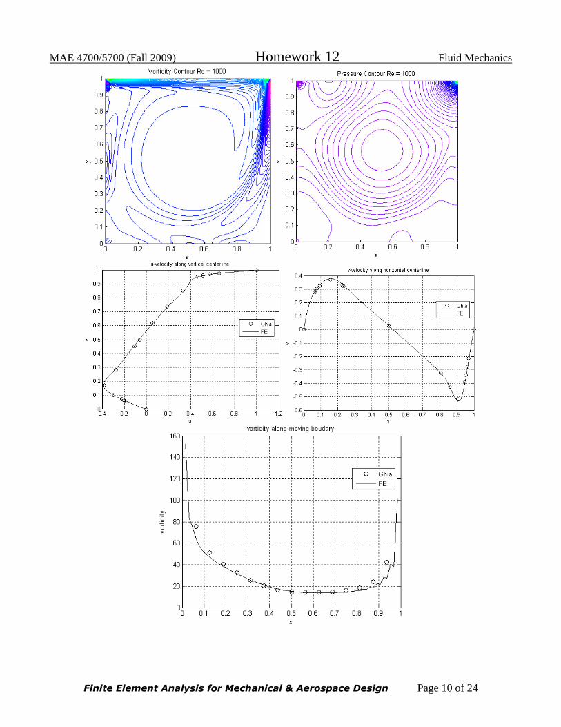
(1) The streamline function, pressure and vorticity contour

(2) The velocity vector plot



(3) Plot u velocity along the line 0.5x , v velocity along the line 0.5y and

vorticity along moving boundary. Compare your results with that listed in

Table I, II and IV of the paper Ghia1.

[1]. U. Ghia, K. N. Ghia and C. T. Shin, “High-resolution for incompressible flow using

the Navier-Stokes equations and multigrid method”, Journal of Computational Physics.

48: 387-411, 1982.

Solution:

Re = 400:

http://cornell.worldcat.org/oclc/1640027&referer=brief_results




Re = 1000:



Problem 3 – Unsteady flow past a circular cylinder at Reynolds number 100

(MatLab)

Simulation of flow past a circular cylinder is one of the most challenging problems in

CFD as unlike other typical numerical tests all the terms in the governing equations are

significant in this case. The problem consists of a circular cylinder immersed in a flowing

viscous fluid. At Reynolds number below about 40, a pair of symmetrical eddies forms

on the downstream side of the cylinder. At higher Reynolds numbers, the symmetrical

eddies become unstable and periodic vortex shedding occurs. The eddies are transported

downstream, resulting in the well-known Karman vortex street.

A Reynolds number of 100 is considered to be the standard for testing FEM algorithms

on the cylinder problem. It is high enough for vortex shedding to occur, but low enough

that the boundary layers can be easily resolved.

The domain and the boundary conditions are shown in the figure. The inlet flow is

uniform and the cylinder is placed at the centerline between two slip walls. The distance

from the inlet and slip walls to the center of the cylinder are 4.5. A no-slip condition is

applied on the cylinder surface. In order to simulate the outflow condition, we take

0p at the outflow (right) boundary. Take time step as 0.05. The initial condition is that

of zero velocity.

Initially, a pair of symmetric attached eddies grew behind the cylinder and the flow reach

a steady state. At this state, the flow has not developed fully yet, and the flow appears

symmetric, with twin vortices forming behind the cylinder. As time progresses, the flow

becomes asymmetric and periodic vortex shedding over the cylinder is attained. In the

present problem, generate your own mesh from ANSYS. Make sure your mesh is fine

enough near the cylinder. Since our code is very stable, you may choose a time step

0.05t and run the problem up to 70.t

(1) Plot the time history of vertical v velocity at the mid-point of exit. Identify the

steady state at t=9 and shedding period . Compute the dimensionless shedding

frequency, or Strouhal number 0

DS

u , where 0 1u in present problem.



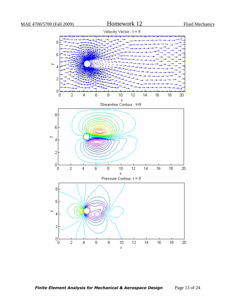
(2) Give the velocity vector plot, pressure, vorticity and streamline contours at the

steady state at t=9. Clearly identify the symmetric twin vortex behind the cylinder.

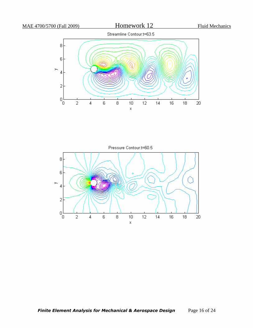
(3) Give the same plots as in (2) during a half period of vortex shedding when the

flow has fully developed yet, i.e. at the beginning, ¼, ½ of the period,. Clearly

identify the asymmetric vortex shedding behind the cylinder.

Compare your results with following two literatures or any other papers you can find:

[2]. T. E. Tezduyar, S. Mittal, S. E. Ray and R. Shih, “Incompressible flow computations

with stabilized bilinear and linear equal-order-interpolation velocity pressure elements”,

Computer Methods in Applied Mechanics and Engineering 95 (1992) 221-242.

[3]. R. Sampath and N. Zabaras, “ A diffpack implementation of the Brooks/Hughes

Streamline-upwind/Petrov-Galerkin FEM formulation of the incompressible Navier-

Stokes equations”, Research Report MM-97-01, Cornell University, March 21. 1997

Solution:

(1) The time history of vertical velocity at the midpoint of exit is:

Therefore, it is clear that after time t=30, the flow has fully developed. The steady state is

achieve around t=9. The shedding period is about 6 .Therefore, the Strouhal number is

10.1667

6S .

(2) The flow achieved steady state at t=9:

0 10 20 30 40 50 60 70-0.4

-0.3

-0.2

-0.1

0

0.1

0.2

0.3Vertical velocity at the middel exit

Time

Velo

city


http://mpdc.mae.cornell.edu/Publications/PDFiles/REPORTS/ns.pdf



It is seen that, at this time, the flow has not developed fully yet, and the flow appears

symmetric, with twin vortices forming behind the cylinder.

(3) From the time history plot, we identify the following three times during half cycle of

the period.



It is seen from the result that at t = 60.5 and t = 63.5, the flow separate at the leading

edge, and the vortex is detached from the cylinder. At t = 62, the growing vortex is ready

to depart from the cylinder.

Problem 4 – Natural convection flow in a cavity (MatLab)



To illustrate the use of the flow in another incompressible flow problem, we shall

describe the splitting-up approximate solution of unsteady natural convection problems.

Such problems involve a coupling between the Navier-Stokes equations describing the

fluid motion and the thermal energy equation governing the space-time evolution of the

temperature. The forces which induce natural convection are in fact spatially variable

gravity forces generated by (buoyancy) density variations in the fluid due to the non-

uniformity of the temperature. The dimensionless equations, in vector form, are

2

2

Pr Pr in [0, ]

0 in [0, ]

in

gp RaT Tt

T

TT T

t

uu u u e

u

u

where Pr is the Prandtl number, Ra is the Rayleigh number and ge is the unit vector in

the direction of gravity.

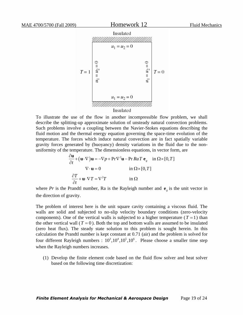
The problem of interest here is the unit square cavity containing a viscous fluid. The

walls are solid and subjected to no-slip velocity boundary conditions (zero-velocity

components). One of the vertical walls is subjected to a higher temperature ( 1T ) than

the other vertical wall ( 0T ). Both the top and bottom walls are assumed to be insulated

(zero heat flux). The steady state solution to this problem is sought herein. In this

calculation the Prandtl number is kept constant at 0.71 (air) and the problem is solved for

four different Rayleigh numbers : 3 4 5 610 ,10 ,10 ,10 . Please choose a smaller time step

when the Rayleigh numbers increases.

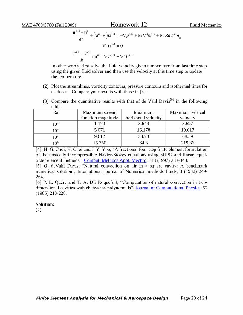
(1) Develop the finite element code based on the fluid flow solver and heat solver

based on the following time discretization:



1

1 1 2 1

1

11 1 2 1

Pr Pr

0

n nn n n n n

g

n

n nn n n

p RaTdt

T TT T

dt

u uu u u e

u

u

In other words, first solve the fluid velocity given temperature from last time step

using the given fluid solver and then use the velocity at this time step to update

the temperature.

(2) Plot the streamlines, vorticity contours, pressure contours and isothermal lines for

each case. Compare your results with those in [4].

(3) Compare the quantitative results with that of de Vahl Davis5,6

in the following

table:

Ra Maximum stream

function magnitude

Maximum

horizontal velocity

Maximum vertical

velocity 310 1.170 3.649 3.697 410 5.071 16.178 19.617 510 9.612 34.73 68.59 610 16.750 64.3 219.36

[4]. H. G. Choi, H. Choi and J. Y. Yoo, “A fractional four-step finite element formulation

of the unsteady incompressible Navier-Stokes equations using SUPG and linear equal-

order element methods”, Comput. Methods Appl. Mechrg, 143 (1997) 333-348.

[5] G. deVahl Davis, “Natural convection on air in a square cavity: A benchmark

numerical solution”, International Journal of Numerical methods fluids, 3 (1982) 249-

264.

[6] P. L. Quere and T. A. DE Roquefort, “Computation of natural convection in two-

dimensional cavities with chebyshev polynomials”, Journal of Computational Physics, 57

(1985) 210-228.

Solution:

(2)

http://www.sciencedirect.com/science?_ob=ArticleURL&_udi=B6V29-3SMTCC6-8&_user=492137&_coverDate=04%2F30%2F1997&_rdoc=8&_fmt=high&_orig=browse&_srch=doc-info(%23toc%235697%231997%23998569996%238590%23FLP%23display%23Volume)&_cdi=5697&_sort=d&_docanchor=&_ct=14&_acct=C000022719&_version=1&_urlVersion=0&_userid=492137&md5=1d595fb2d7ef0e43406ae5b3a8794f07

http://www.sciencedirect.com/science?_ob=ArticleURL&_udi=B6WHY-4DD1YSB-20P&_user=492137&_coverDate=01%2F30%2F1985&_rdoc=3&_fmt=high&_orig=browse&_srch=doc-info(%23toc%236863%231985%23999429997%23520868%23FLA%23display%23Volume)&_cdi=6863&_sort=d&_docanchor=&_ct=9&_acct=C000022719&_version=1&_urlVersion=0&_userid=492137&md5=92822b666d6b9964ab37181857fa0e6d



Discussion:

For Ra = 103 and 10

4 no distinct boundary layers can be seen. The flow at Ra = 10

4

shows the onset of a stratified core in the cavity, a behavior characteristic of higher

Rayleigh number flows. At Ra = 105 three major changes can be seen:

1. Secondary circulation exists in the core.

2. There is a substantial temperature gradient near the vertical walls.

3. The lower and upper right corners have become much more active than the other

two.

Also, it is expected that the pressure field is influenced by the For high Ra the pressure

becomes more uniform across the cavity, except near the corners. The vorticity plots

generally show a central negative area (rotation in the direction of the main circulation)

separated by a zero contour from positive vorticity regions adjacent to the walls. By Ra =



104

there are two distinct valleys of vorticity in the central area; with increasing Ra these

move apart, leaving a central area with little action.

(3) The finite element solution is :

Ra Maximum stream

function magnitude

Maximum

horizontal velocity

Maximum vertical

velocity 310 1.17285 3.64601 3.70729 410 5.07381 16.2511 19.6964 510 9.60661 43.9062 68.9105 610 16.7319 127.767 216.763

From the table, the finite element solutions are accurate for low Rayleigh numbers. For

high Rayleigh numbers, the horizontal velocity lost accuracy. This is possibly due to the

lack of stabilization of the convection terms since in these cases the magnitude of the

velocity is quite big. Therefore, it is possible to add SUPG onto the current algorithm to

make the solution more stable.

MAE 4700/5700 (Fall 2009) Homework 12 Fluid...

Documents

Transcript of MAE 4700/5700 (Fall 2009) Homework 12 Fluid...