MAE 123 : Mechanical Engineering Laboratory II …jmmeyers/ME123/Lectures/ME123 Lecture 1...MAE 123...
29
MAE 123 : Mechanical Engineering Laboratory II Introduction to Experimental Practice MAE 123 : Mechanical Engineering Laboratory II Introduction to Experimental Practice Dr. J. M. Meyers | Dr. D. G. Fletcher | Dr. Y. Dubief Image: wot.nasa.gov 1
-
Upload
trinhtuong -
Category
Documents
-
view
216 -
download
2
Transcript of MAE 123 : Mechanical Engineering Laboratory II …jmmeyers/ME123/Lectures/ME123 Lecture 1...MAE 123...

MAE 123 : Mechanical Engineering Laboratory II
Introduction to Experimental Practice
MAE 123 : Mechanical Engineering Laboratory II
Introduction to Experimental PracticeDr. J. M. Meyers | Dr. D. G. Fletcher | Dr. Y. Dubief
Image: wot.nasa.gov 1

MAE 123 : Mechanical Engineering Laboratory II
Introduction to Experimental Practice
I. Error
Illegitimate error
Random error
Systematic error
II. Accuracy and Precision
Accuracy
Precision (Relative and Absolute)
Significant Digits
III. Propagation of Error: Uncertainty
IV. Parameter Sensitivity
by differentiation
by logarithmic differentiation
V. Presentation of Scientific Data
OUTLINE
2
MAE 123 : Mechanical Engineering Laboratory II
Introduction to Experimental Practice
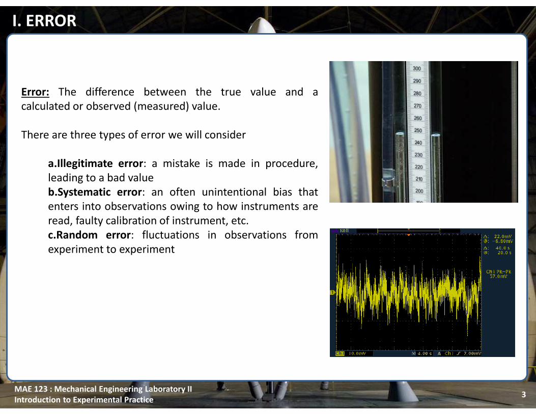
Error: The difference between the true value and a
calculated or observed (measured) value.
There are three types of error we will consider
a.Illegitimate error: a mistake is made in procedure,
leading to a bad value
b.Systematic error: an often unintentional bias that
enters into observations owing to how instruments are
read, faulty calibration of instrument, etc.
c.Random error: fluctuations in observations from
experiment to experiment
I. ERROR
3
MAE 123 : Mechanical Engineering Laboratory II
Introduction to Experimental Practice
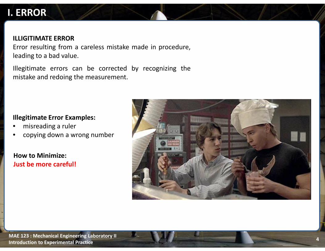
ILLIGITIMATE ERROR
Error resulting from a careless mistake made in procedure,
leading to a bad value.
I. ERROR
Illegitimate errors can be corrected by recognizing the
mistake and redoing the measurement.
4
Illegitimate Error Examples:
• misreading a ruler
• copying down a wrong number
How to Minimize:
Just be more careful!

MAE 123 : Mechanical Engineering Laboratory II
Introduction to Experimental Practice
SYSTEMATIC ERROR
I. ERROR
Systematic errors can be eliminated only by critical examination
of the experimental method, and often this is accomplished by
performing an experiment with the apparatus to measure a
known or analytically determined value. Another approach is to
have a different person perform the same experiment!
5
Systematic Error Examples
• The cloth tape measure that you use to measure the length of an object had been stretched out
from years of use. (As a result, all of your length measurements were too small.)
• The electronic scale you use reads 0.05 g too high for all your mass measurements (because it is
improperly tared throughout your experiment).
• Using a timer that is slow, so that all the times measured are slow by the same factor.
How to minimize
Systematic errors are difficult to detect and cannot be analyzed statistically, because all of the data is
off in the same direction (either to high or too low). Spotting and correcting for systematic error takes
a lot of care.
• How would you compensate for the incorrect results of using the stretched out tape measure?
• How would you correct the measurements from improperly tared scale?
Owes to unintentional bias that enters into observations due to
how instruments are read, faulty calibration of instrument, etc.
A reproducible error that biases the data in a given direction.

MAE 123 : Mechanical Engineering Laboratory II
Introduction to Experimental Practice
Fluctuations in observations from experiment to experiment
that follow statistical distributions.
I. ERROR
Random errors are not something that can be controlled and
are typically present owing to limitations on instrumentation
or to an inability to completely control the test conditions.
6
Random Error Examples:
• You measure the mass of a ring three times using the same balance and get slightly different values:
17.46 g, 17.42 g, 17.44 g
• Noise in an oscilloscope reading
How to minimize or eliminate random errors:
• Take more data. Random errors follow statistical distributions thus can be evaluated through
statistical analysis and can be reduced by averaging over a large number of observations.
RANDOM ERROR
Random error is not the fault of you or the equipment

MAE 123 : Mechanical Engineering Laboratory II
Introduction to Experimental Practice
ACCURACY: a measure of how close the experimental (or
calculated) value is to the true value
PRECISION: a measure of how exactly the experimental
result is determined without reference to what the result
means. Precision is also a measure of how reproducible the
result is.
Absolute precision: indicates magnitude of uncertainty in
the same units as the result
Relative precision: indicates the uncertainty as a fraction
of the value of the result.
From the definitions it is clear that accuracy ≠ precision
The precision of an experimental observation determines the
number of significant digits used to report the value -- points
will be deducted for using too many digits to report an
answer.
II. ACCURACY AND PRECISIONII. ACCURACY AND PRECISION
7

MAE 123 : Mechanical Engineering Laboratory II
Introduction to Experimental Practice
SIGNIFICANT DIGITS:
a. Left-most non-zero digit is most significant digit
b. If no decimal point, right-most non-zero digit is least
significant digit
c. If decimal point right-most, digit is least significant even if 0
d. All digits between least and most significant count as
significant digits
8
•Reporting in scientific notation makes it easier to keep track of significant digits in calculations
•Quoting result of experiment should use one figure more than determined by experimental
precision
•In calculations keep this extra digit for each variable, so that the final result retains equivalent
precision from all input
II. ACCURACY AND PRECISION
1,234
123,400
123.4
1,001
1,000.
10.10
0.0001010
1.234(10)3
1.234(10)6
1.234(10)2
1.001(10)3
1.000(10)3
1.010(10)1
1.010(10)-4
All numbers below have 4 significant
digits by the above rules.
In many cases it is beneficial
to use scientific notation
How many significant
digits does this readout
have?
What would be its
representation in
scientific notation?

MAE 123 : Mechanical Engineering Laboratory II
Introduction to Experimental Practice
A student measures table top with steel meter rule and finds an average value of 1.982 m for the
length.
This student finds after that the rule was calibrated at 25 C, and has an expansion coefficient of
0.0005/C.
The experiment was done at 20 C, so the student multiplies result by 1-5(0.0005) = 0.9975, so his
result is now 1.977 m.
This illustrates a systematic error due to incorrect calibration and how this particular systematic
error can be corrected.
The table manufacturer lists the table at a length of L = 2.000 m. This means the result is
inaccurate by 23 mm.
II. ACCURACY AND PRECISION
9
Example 1: Tabletop Measurement Error, Precision, and Accuracy
Precision: reported length is precise 1.977 m.
Represented significant digits Imply measurement has an absolute precision of 1 mm. (relative
precision on the order of 1/1977)
MAE 123 : Mechanical Engineering Laboratory II
Introduction to Experimental Practice
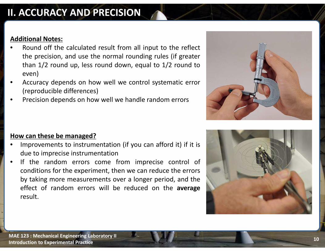
Additional Notes:
• Round off the calculated result from all input to the reflect
the precision, and use the normal rounding rules (if greater
than 1/2 round up, less round down, equal to 1/2 round to
even)
• Accuracy depends on how well we control systematic error
(reproducible differences)
• Precision depends on how well we handle random errors
How can these be managed?
• Improvements to instrumentation (if you can afford it) if it is
due to imprecise instrumentation
• If the random errors come from imprecise control of
conditions for the experiment, then we can reduce the errors
by taking more measurements over a longer period, and the
effect of random errors will be reduced on the average
result.
10
II. ACCURACY AND PRECISION

MAE 123 : Mechanical Engineering Laboratory II
Introduction to Experimental Practice
•Generally, the result of our experiment is an estimate of the true value.
•We can only estimate the errors since we often do not know the true value in advance
•Repeating experiment often gives a different result, so we look to see if the results agree within
estimated uncertainty.
•Repeating the experiment to reduce influence of random errors means we will usually estimate a
mean and standard deviation for the data -- statistical analysis
Usually, the result we are looking for in an experiment is determined from a combination of
measurements. Thus, the uncertainty in the result is determined by the uncertainty in the separate
measurements. What is this dependence?
11
III. PROPAGATION OF ERROR: UNCERTAINTY

MAE 123 : Mechanical Engineering Laboratory II
Introduction to Experimental Practice
� � = 12��� exp − � − �
2��
Measured data with only random error contributions follow a normal (aka Gaussian) distribution with
parameters and �. This probability density function is given by:
12
III. PROPAGATION OF ERROR: UNCERTAINTY
�� ≡ variance� ≡ standarddeviation ≡ meanvalue
FWHM = 2σ −2ln 1/2-2.0 -1.5 -1.0 -0.5 0.0 0.5 1.0 1.5 2.0
0
1
2
3
4
FWHM
FWHMf(x)
x
µ = 0, σ = 0.1 µ = -1, σ = 0.1 µ = 0, σ = 0.5
FWHM
MAE 123 : Mechanical Engineering Laboratory II
Introduction to Experimental Practice
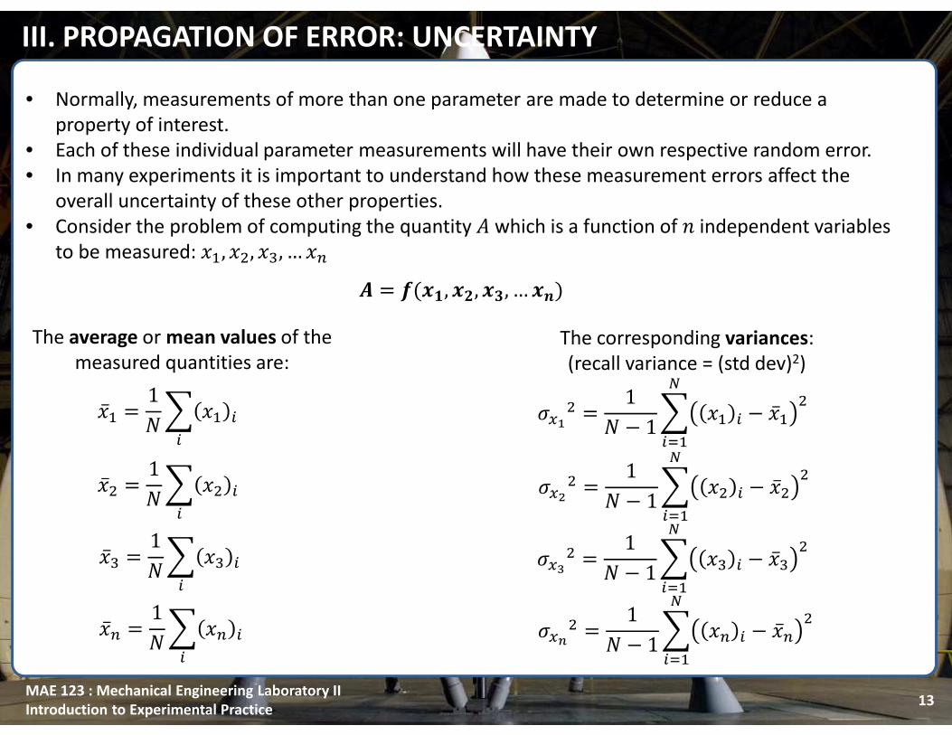
• Normally, measurements of more than one parameter are made to determine or reduce a
property of interest.
• Each of these individual parameter measurements will have their own respective random error.
• In many experiments it is important to understand how these measurement errors affect the
overall uncertainty of these other properties.
• Consider the problem of computing the quantity # which is a function of $ independent variables
to be measured: �%, ��, �', … �)* = +(-., -/, -0, … -1)
13
�̅% =145 �% 6
6
�̅� =145 �� 6
6
�̅' =145 �' 6
6
�̅) =145 �) 6
6
�78� =1
4 − 15 �% 6 − �̅% �9
6:%
�7;� =1
4 − 15 �� 6 − �̅� �9
6:%
�7<� =1
4 − 15 �' 6 − �̅' �9
6:%
�7=� =1
4 − 15 �) 6 − �̅) �9
6:%
III. PROPAGATION OF ERROR: UNCERTAINTY
The average or mean values of the
measured quantities are:
The corresponding variances:
(recall variance = (std dev)2)

MAE 123 : Mechanical Engineering Laboratory II
Introduction to Experimental Practice14
#6 − #̅ ≈ �% 6 − �̅%?#?�% 7;,7<,…7=
+ �� 6 − �̅�?#?�� 78,7<,…7=
+ �' 6 − �̅'?#?�' 78,7;,…7=
+⋯+ �) 6 − �̅)?#?�) 78,7;,7<,…7=B8
Each combination of measurements can be used to estimate the deviation from the average value
using a Taylor Series expansion:
For illustration simplicity, let’s assume our desired parameter # is a function of just two measured
quantities, �% and ��:
III. PROPAGATION OF ERROR: UNCERTAINTY
#6 − #̅ ≈ �% 6 − �̅%?#?�% 7;
+ �� 6 − �̅�?#?�� 78

MAE 123 : Mechanical Engineering Laboratory II
Introduction to Experimental Practice15
If we square both sides and sum over all measurements, then we can replace the difference terms by
variances (��). How many terms are there on RHS?
III. PROPAGATION OF ERROR: UNCERTAINTY
�D� = �78�?#?�% 7;
�+ 24 − 15 �% 6 − �̅%
?#?�% 7;
�� 6 − �̅�?#?�� 78
9
6:%+ �7;�
?#?�� 78
�
Here we usually assume that the two variable “errors” are not related -- that they are statistically
independent. This is the most common situation. If a large enough sample set is then taken, any
covariance term will be zero:
�D� = �78�?#?�%
�+ �7;�
?#?��
��D = �78�
?#?�%
�+ �7;�
?#?��
�
=0
But what about calculated parameters that are a function of more than two measurements?
Thus only two RHS terms will remain. With the assumption of independence our estimate of the
variance of the derived result is then:
5�7=�7E9
%= 0

MAE 123 : Mechanical Engineering Laboratory II
Introduction to Experimental Practice16
In fact, it can be shown that for a desired parameter that is a function of $ number of measured
quantities:
III. PROPAGATION OF ERROR: UNCERTAINTY
# = �(�%, ��, �', … �))
�D = �78�?#?�%
�+ �7;�
?#?��
�+ �7<�
?#?�'
�+⋯+ �7=�
?#?�)
�
that all the cross terms will cancel and the total uncertainty of parameter # can then be derived from
the following relation:
Let’s apply this to a couple of examples...
Error in
measurement
of �%
Error in
measurement
of ��
Error in
measurement
of �'
Error in
measurement
of �)
Partial derivatives of calculated parameter # with respect to individual measured parameter while
holding other measured parameters constant under assumption of statistical independence
General Form for
the Expression of
Uncertainty

MAE 123 : Mechanical Engineering Laboratory II
Introduction to Experimental Practice17
III. PROPAGATION OF ERROR: UNCERTAINTY
We now want to estimate how far we probably are from this value owing to the imprecision of our
measurements (we hope we have eliminated systematic errors and that we are only dealing with
random errors -- we checked the thermometer and pressure transducer for proper calibration.)
G = HIJWe want to determine the density of room air, which is very difficult to measure directly. We recall
the ideal gas law:
H = GIJ
As we are working with air, we know that:
I = IK)6L/(MW)= 8.3145 N-m/(mol K)/0.029 kg/mol = 287.0 (N-m)/(kg-K).
We take turns reading the thermometer and find an average value for room J of 298 K, with a
standard deviation of �M = 2 K.
We also use a pressure transducer to measure the ambient condition, and after repeating this many
times find an average value of G = 101000 N/m2 with a standard deviation of �N= 100 N/m2.
H = GIJ =
101000(287.0)(298) = 1.18kg/m
3
Example 2: Measurement of Density (1/2)

MAE 123 : Mechanical Engineering Laboratory II
Introduction to Experimental Practice18
III. PROPAGATION OF ERROR: UNCERTAINTY
We have only two measurements in calculating H (pressure, G, and temperature, J). Using the
derived general form for the expression of uncertainty (Slide 15) we obtain:
�V = �M�?H?J
�+ �N�
?H?G
�
?H?J = −
12GIJ�
?H?G =
1IJ
�V = �M� −12GIJ�
�+ �N�
1IJ
�
�V = 2� −12101000
287.0(298)��+ (100)� 1
287.0(298)�
�V =4.13(10)-3 kg/m3
H = 1.18 ± 4.13 10 −3 kg/m3
Example 2: Measurement of Density (2/2)
The partial differentials of each measured quantity while holding the other measure quantity as
constant are:
Substituting these relations into our relation for uncertainty:
Adding our measured values and working through we obtain:
or

MAE 123 : Mechanical Engineering Laboratory II
Introduction to Experimental Practice19
III. PROPAGATION OF ERROR: UNCERTAINTY
G + 12HY� + HZ[ = constant
The Bernoulli principle is a very useful concept in fluid dynamics because it is easy to use and can give
great insight into the balance between pressure, velocity and elevation. Simply stated, at any point
along a streamline of fluid flow, the summation of pressure, dynamic pressure, and head pressure will
be constant.
Assuming the two measurement points (1 and 2) are at the same elevation ([% ≈ [�):
G% +12H%Y%
� = G� +12H�Y�
�
Example 3: Pitot Probe Measurement (1/3)
This is the key relation in extracting fluid velocity from an instrument called a Pitot probe.

MAE 123 : Mechanical Engineering Laboratory II
Introduction to Experimental Practice20
III. PROPAGATION OF ERROR: UNCERTAINTY
Example 3: Pitot Probe Measurement (2/3)
G% +12H%Y%
� = G� +12H�Y�
�
At the static pressure port (location 1), the velocity is normally taken to be 0 as this measurement is
perpendicular to the flow direction (ergo no dynamic pressure):
0
Solving for velocity at measurement point 2:
Y� = 2 (G% − G�)H�
It is common practice to measure a pressure
difference rather than the two pressure values,
thus:
Y� =2∆GH�
MAE 123 : Mechanical Engineering Laboratory II
Introduction to Experimental Practice21
III. PROPAGATION OF ERROR: UNCERTAINTY
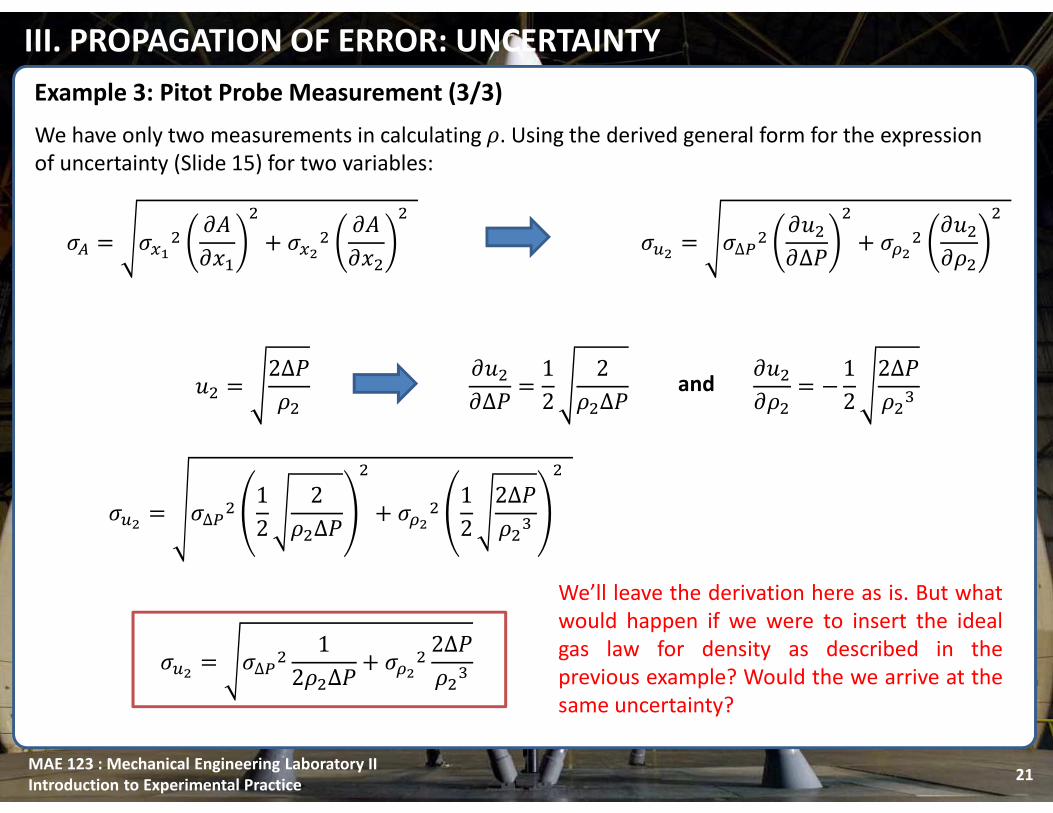
Example 3: Pitot Probe Measurement (3/3)
We have only two measurements in calculating H. Using the derived general form for the expression
of uncertainty (Slide 15) for two variables:
?Y�?∆G =
12
2H�∆G
?Y�?H� = −
122∆GH�'
�D = �78�?#?�%
�+ �7;�
?#?��
� �K; = �∆N�
?Y�?∆G
�+ �V;�
?Y�?H�
�
Y� =2∆GH�
�K; = �∆N�12
2H�∆G
�
+ �V;�122∆GH�'
�
�K; = �∆N�1
2H�∆G + �V;� 2∆GH�'
and
We’ll leave the derivation here as is. But what
would happen if we were to insert the ideal
gas law for density as described in the
previous example? Would the we arrive at the
same uncertainty?

MAE 123 : Mechanical Engineering Laboratory II
Introduction to Experimental Practice
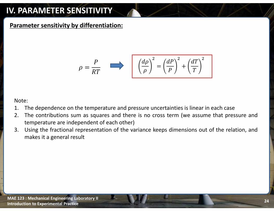
Parameter sensitivity by differentiation:
In our density calculation from Example 2 recall that:
These relations express the fractional change in density caused by a fractional change in the two
independent variables, G and J. These express the non-dimensional sensitivities of density to the
two variables.
To find the pressure sensitivity, we differentiate the expression w.r.t. G, keeping J constant, and
then w.r.t. to J keeping G constant.
Replacing the partial terms with the full differential, we can rearrange the two relations into more
convenient, intuitive forms:
22
IV. PARAMETER SENSITIVITY
H = GIJ
?H?G M
= 1IJ =
GIJ1G =
HG
?H?J N
= − GIJ� = −
GIJ1J = −
HJ
]HH =
]GG
]HH = −
]JJ

MAE 123 : Mechanical Engineering Laboratory II
Introduction to Experimental Practice
Now going back to Example 2 again our general relation for density depending on BOTH temperature
and pressure is:
Using the partial differentials from the previous slide and if we let:
Dividing both sides by density squared yields the following:
23
IV. PARAMETER SENSITIVITY
Parameter sensitivity by differentiation:
�V� = �M�?H?J
�+ �N�
?H?G
�
�V = ]H �N = ]G �M = ]J
]H� = ]J� −HJ�+ ]G� HG
�We then arrive at:
]HH
�= ]G
G�+ ]J
J�
MAE 123 : Mechanical Engineering Laboratory II
Introduction to Experimental Practice
Note:
1. The dependence on the temperature and pressure uncertainties is linear in each case
2. The contributions sum as squares and there is no cross term (we assume that pressure and
temperature are independent of each other)
3. Using the fractional representation of the variance keeps dimensions out of the relation, and
makes it a general result
24
IV. PARAMETER SENSITIVITY
]HH
�= ]G
G�+ ]J
J�
H = GIJ
Parameter sensitivity by differentiation:

MAE 123 : Mechanical Engineering Laboratory II
Introduction to Experimental Practice
We then differentiate term-by-term, and this produces the fractional variances directly, with the
proper sensitivity scaling.
Another approach provides a short cut for differentiation. We take the natural log of both sides of
the expression:
We now square both sides, and assume that the cross term is zero (recall the assumption of
independent measurements of the separate parameters, G and J). This yields the same result as
the formal approach:
25
IV. PARAMETER SENSITIVITY
Parameter sensitivity by logarithmic differentiation:
ln H = ln G − ln I − ln JH = GIJ
]HH =
]GG −
]JJ
]HH
�= ]G
G�− 2 ]G
G]JJ + ]J
J�
0
]HH
�= ]G
G�+ ]J
J�

MAE 123 : Mechanical Engineering Laboratory II
Introduction to Experimental Practice26
V. PRESENTATION OF SCIENTIFIC DATA
Measurements are normally displayed and represented in Tables or Graphs.
Units of each listed value must be included.
0 50 100 150 200 250 300 350 400 450
20
40
60
80
100
120
140
160
180
Water Temperature Heater Temperature
Tem
pera
utre
[C
]
Time [s]
Time
Water
Temperature
Heater
Temperature
[s] [C] ±3 [C] ±10
30 17 120
60 18 123
90 20 125
120 22 128
150 24 132
180 25 120
210 24 142
240 22 135
270 18 141
300 16 145
330 20 147
360 22 154
390 24±4 152
420 21±1 157
Graphs:
• Both axes must include measurement label
and unit
• Error bars for each representative data point
must be graphically illustrated
• If more than one data record is being
represented, an appropriate legend must be
used.
• Scale axes accordingly to represent what you
are trying to illustrate with your graph
Tables:
• Each column must include a header
measurement label and unit
• Error can either be represented in the
column header (if universal)
• If error is not universal the value must be
represented for each data point

MAE 123 : Mechanical Engineering Laboratory II
Introduction to Experimental Practice27
V. PRESENTATION OF SCIENTIFIC DATA
Measurements are normally displayed and represented in Tables or Graphs.
Units of each listed value must be included.
0 50 100 150 200 250 300 350 400 450
20
40
60
80
100
120
140
160
180
Water Temperature Heater Temperature
Tem
pera
utre
[C
]
Time [s]
Time
Water
Temperature
Heater
Temperature
[s] [C] ±3 [C] ±10
30 17 120
60 18 123
90 20 125
120 22 128
150 24 132
180 25 120
210 24 142
240 22 135
270 18 141
300 16 145
330 20 147
360 22 154
390 24±4 152
420 21±1 157
Graphs:
• Both axes must include measurement label
and unit
• Error bars for each representative data point
must be graphically illustrated
• If more than one data record is being
represented, an appropriate legend must be
used.
• Scale axes accordingly to represent what you
are trying to illustrate with your graph
Tables:
• Each column must include a header
measurement label and unit
• Error can either be represented in the
column header (if universal)
• If error is not universal the value must be
represented for each data point

MAE 123 : Mechanical Engineering Laboratory II
Introduction to Experimental Practice28
GLOSSARY OF TERMS
Accuracy (of measurement) Closeness of agreement between a measured value and a true value. The term "precision" should not be
used for "accuracy".
Decimal places -the number of digits to the right of the decimal point.
Discrepancy - A significant difference between two measured values of the same quantity.
Error (of measurement) The inevitable uncertainty inherent in measurements
Illegitimate error- mistake or blunder - a procedural error that should be avoided by careful
Law of propagation of uncertainty - shows how the uncertainties (not the errors) of the input quantities combine
Precision - The degree of refinement with which an operation is performed or a measurement stated [Webster].
Random error -Statistical fluctuations (in either direction) in the measured data due to the precision limitations of the measurement
device.
Relative error- Error of measurement divided by a true value of the measurement. Relative error is often reported as a percentage.
Significant figures - all digits between and including the first non-zero digit from the left, through the last digit .
Systematic error -A reproducible inaccuracy introduced by faulty equipment, calibration, or technique. Unlike random errors,
systematic errors cannot be reduced by increasing the number of observations nor do they follow random error’s statistical trend.
True value (of a quantity) The value that is approached by averaging an increasing number of measurements with no systematic
errors.
Uncertainty (of measurement) Associated with the result of a measurement, that characterizes the dispersion of the values that could
reasonably be attributed to the measurand. The uncertainty generally includes many components which may be evaluated from
experimental standard deviations based on repeated observations.
Absolute uncertainty The total uncertainty of a value.
Relative (fractional) uncertainty - the absolute uncertainty divided by the measured value, often expressed as a
percentage.
MORE TO COME…
MAE 123 : Mechanical Engineering Laboratory II
Introduction to Experimental Practice
REFERENCES AND FURTHER READING
1) T. Arts, H. Boerrigter, J.-M. Buchlin, M. Carbonaro, G. Degrez, R. Denos, D. Fletcher, D. Olivari, M. L.
Riethmuller, and R. A. van den Braembussche, “Measurement Techniques in Fluid Dynamics,” von Karman
Institute for Fluid Dynamics, 2nd Revised Edition.
2) E. O. Doebelin, “Measurement Systems: Application and Design,” McGraw-Hill Book Company, 1983, New
York
3) H. H. Ku, “Notes on the use of propagation of error of formulas,” Journal of Research of the National Bureau
of Standards, 70C (4):262
4) P. R. Bevington, “Data Reduction and Error Analysis for the Physical Sciences,”
Image: wot.motortrend.com 29