Saddle Point Methods forOption Pricing

Dilip B. MadanRobert H. Smith School of Business

Joint work with Peter Carr

June 19 2009Spectral and Cubature Methods in

Financial EconometricsUniversity of Leicester

1

Motivation• Many models are formulated for thelogarithm of the stock price with a tractablecharacteristic function in the exponentialaffine class, Duffie, Pan and Singleton(2000).

• These models may then be calibrated usingthe Fourier methods of Carr and Madan(1999).

2

• Unfortunately these methods break downfor deep out of the money option prices.

• Rogers and Zane (1999), Xiong, Wongand Salopek (2005) propose saddlepointmethods for option prices.

• These are appropriate as saddlepoint meth-ods are classically designed to computevery small tail probabilities.

• The papers by Rogers and Zane (1999) andXiong, Wong and Salopek (2005) proposeusing saddlepoint methods for the twoprobabilities required, stock exceeds strikerisk neutrally and stock exceeds strikeunder the share measure.

• Two saddlepoint approximations arethereby needed for one option price.

3

Our Strategy• In Carr and Madan (1999) we replaced twoFourier inversions for one option price withone inversion for one option price.

•We do the same here for saddlepointmethods.

•We begin by noting that the call pricerelative to the spot price of the stock is theprobability that under the share measure thelogarithm of the stock exceeds log strike byan independent exponential variate.

• Hence we need to compute just this one tailprobability for the call price.

4

Some implications• Even in the classical Black Scholes casethe classical saddlepoint methods usingGaussian bases are not exact for the callprice computed as a single probability.

• The exact base is the distribution of aGaussian variate less an independentpositive exponential.

•We extend the non-Gaussain base saddle-point methods of Wood, Booth and Butler(1993) with our suggested base to developexact saddlepoint pricing in the BlackScholes case, and then apply the same toother models.

• The models considered are CGMY,CGY SN , V GSSD, SV J, HSV andV GSA.

5

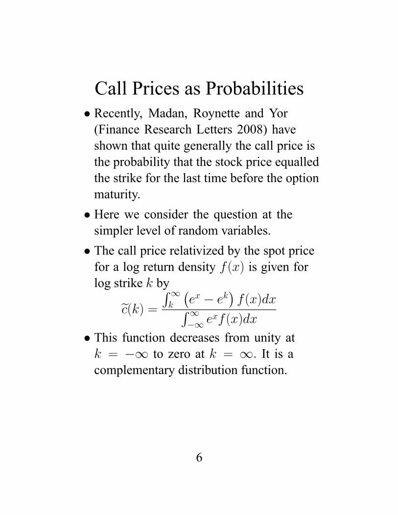
Call Prices as Probabilities• Recently, Madan, Roynette and Yor(Finance Research Letters 2008) haveshown that quite generally the call price isthe probability that the stock price equalledthe strike for the last time before the optionmaturity.

• Here we consider the question at thesimpler level of random variables.

• The call price relativized by the spot pricefor a log return density f(x) is given forlog strike k by

ec(k) = R∞k ¡ex − ek

¢f(x)dxR∞

−∞ exf(x)dx

• This function decreases from unity atk = −∞ to zero at k = ∞. It is acomplementary distribution function.

6

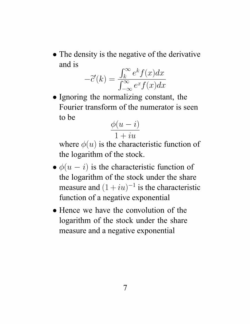
• The density is the negative of the derivativeand is

−ec0(k) = R∞k ekf(x)dxR∞−∞ exf(x)dx

• Ignoring the normalizing constant, theFourier transform of the numerator is seento be

φ(u− i)

1 + iuwhere φ(u) is the characteristic function ofthe logarithm of the stock.

• φ(u − i) is the characteristic function ofthe logarithm of the stock under the sharemeasure and (1+ iu)−1 is the characteristicfunction of a negative exponential

• Hence we have the convolution of thelogarithm of the stock under the sharemeasure and a negative exponential

7

The Density embedded in CallPrices

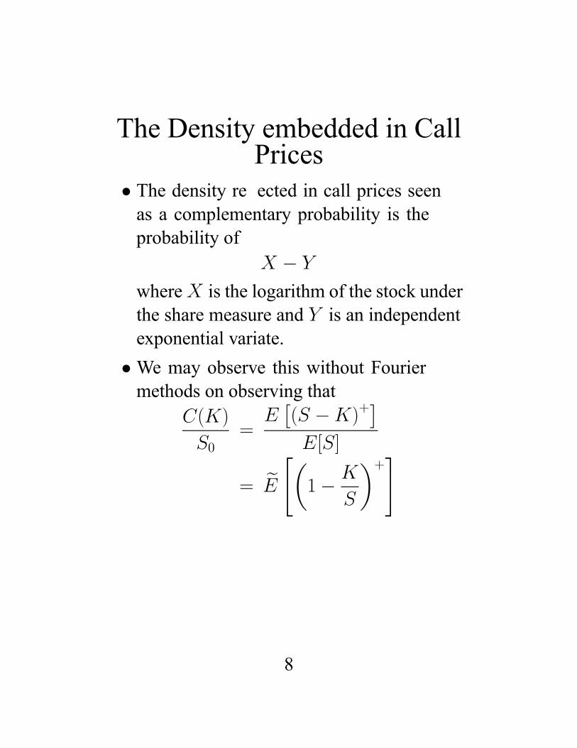
• The density re�ected in call prices seenas a complementary probability is theprobability of

X − Y

whereX is the logarithm of the stock underthe share measure and Y is an independentexponential variate.

•We may observe this without Fouriermethods on observing that

C(K)

S0=

E£(S −K)+

¤E[S]

= eE "µ1− K

S

¶+#

8

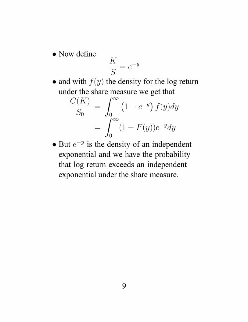
• Now defineK

S= e−y

• and with f(y) the density for the log returnunder the share measure we get that

C(K)

S0=

Z ∞0

¡1− e−y

¢f(y)dy

=

Z ∞0

(1− F (y))e−ydy

• But e−y is the density of an independentexponential and we have the probabilitythat log return exceeds an independentexponential under the share measure.

9

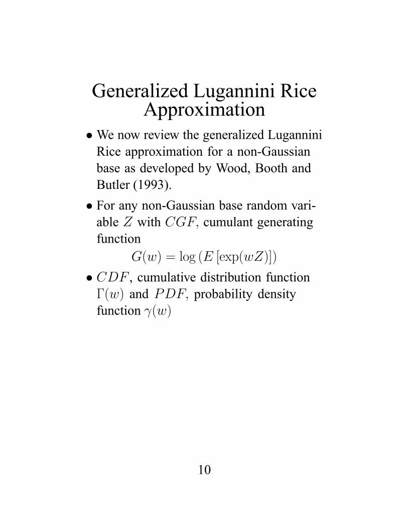
Generalized Lugannini RiceApproximation

•We now review the generalized LuganniniRice approximation for a non-Gaussianbase as developed by Wood, Booth andButler (1993).

• For any non-Gaussian base random vari-able Z with CGF, cumulant generatingfunction

G(w) = log (E [exp(wZ)])

• CDF , cumulative distribution functionΓ(w) and PDF, probability densityfunction γ(w)

10

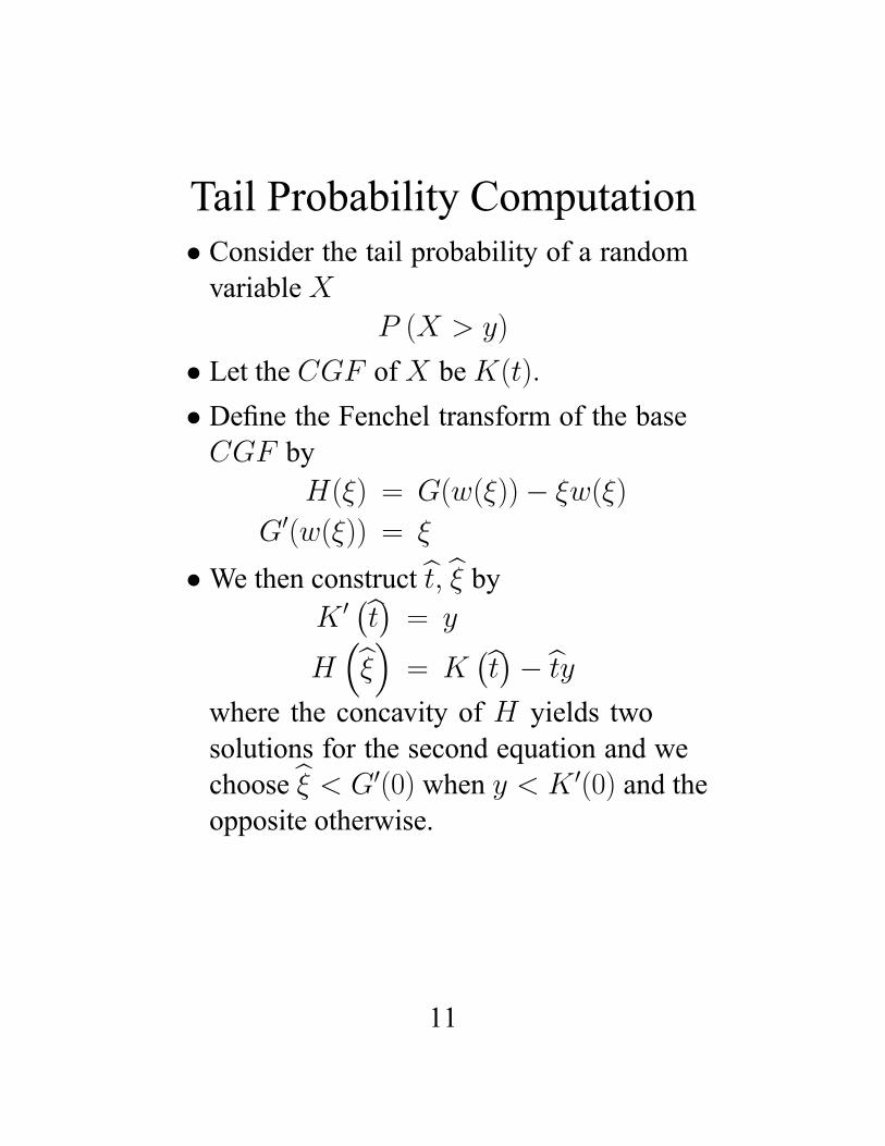
Tail Probability Computation• Consider the tail probability of a randomvariableX

P (X > y)

• Let the CGF ofX beK(t).• Define the Fenchel transform of the baseCGF by

H(ξ) = G(w(ξ))− ξw(ξ)

G0(w(ξ)) = ξ

•We then construct bt, bξ byK 0 ¡bt¢ = y

H³bξ´ = K

¡bt¢− btywhere the concavity of H yields twosolutions for the second equation and wechoose bξ < G0(0) when y < K 0(0) and theopposite otherwise.

11

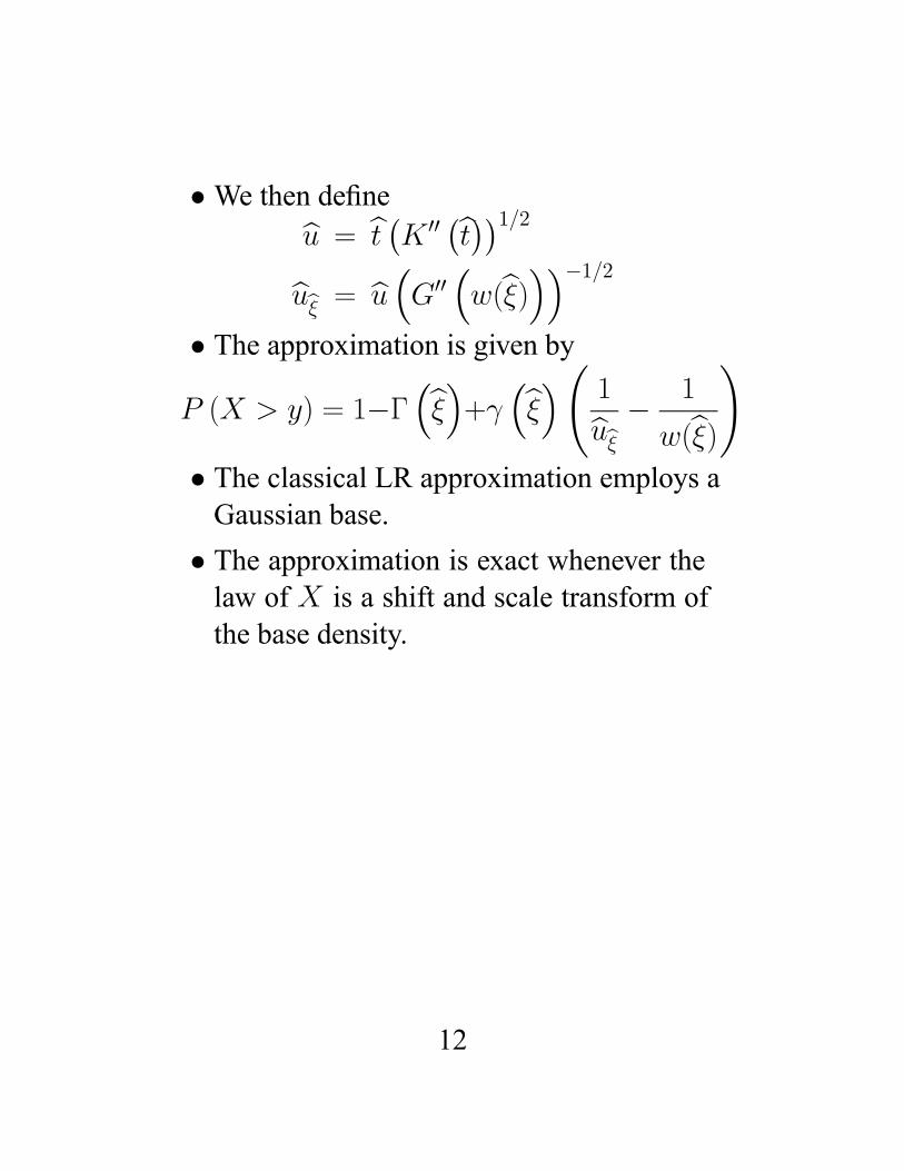
•We then definebu = bt ¡K 00 ¡bt¢¢1/2bubξ = bu³G00 ³w(bξ)´´−1/2

• The approximation is given byP (X > y) = 1−Γ

³bξ´+γ ³bξ´Ã 1bubξ − 1

w(bξ)!

• The classical LR approximation employs aGaussian base.

• The approximation is exact whenever thelaw of X is a shift and scale transform ofthe base density.

12

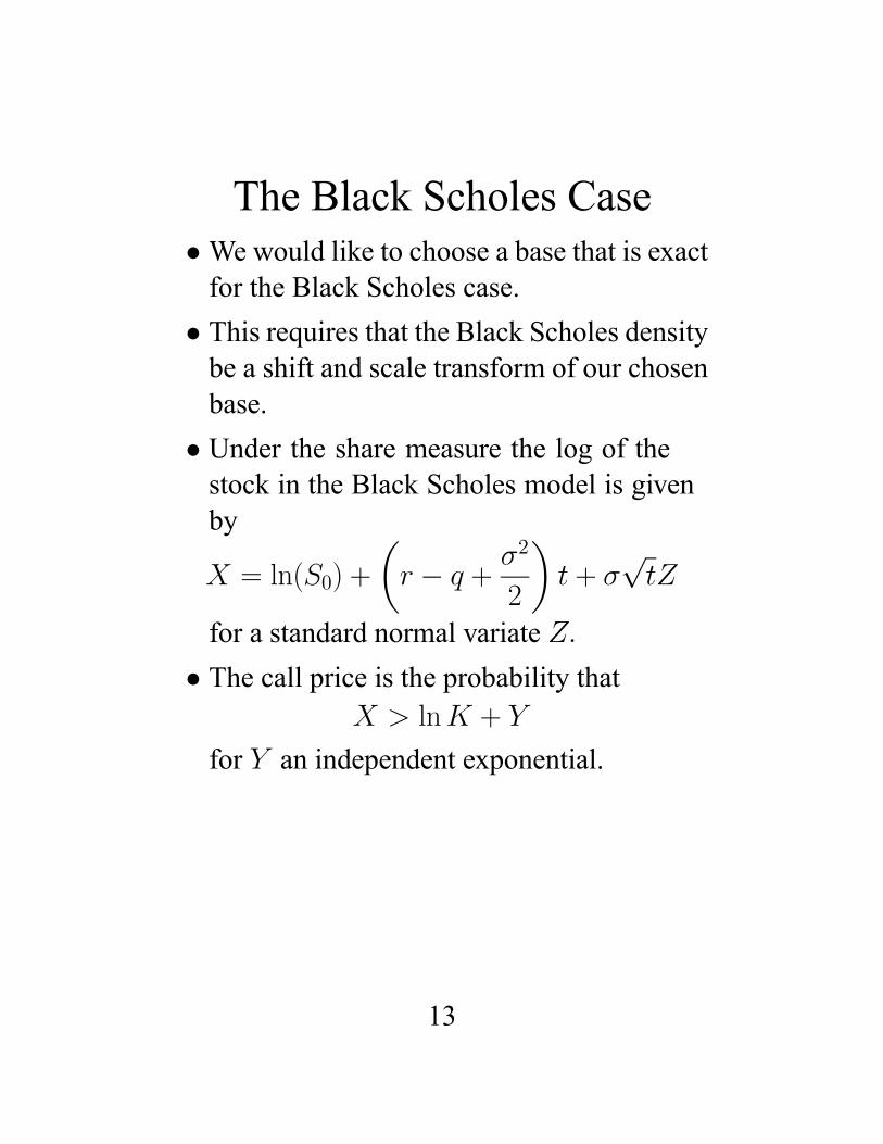
The Black Scholes Case•We would like to choose a base that is exactfor the Black Scholes case.

• This requires that the Black Scholes densitybe a shift and scale transform of our chosenbase.

• Under the share measure the log of thestock in the Black Scholes model is givenby

X = ln(S0) +

µr − q +

σ2

2

¶t + σ

√tZ

for a standard normal variate Z.• The call price is the probability that

X > lnK + Y

for Y an independent exponential.

13

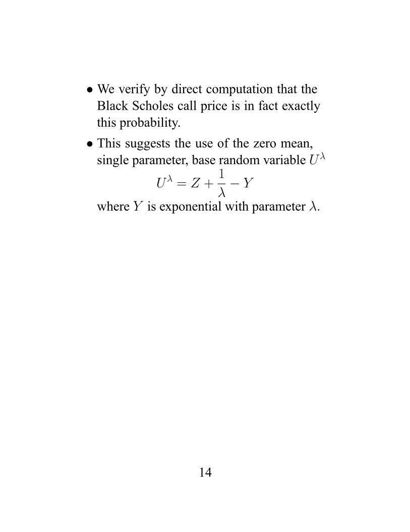
•We verify by direct computation that theBlack Scholes call price is in fact exactlythis probability.

• This suggests the use of the zero mean,single parameter, base random variable Uλ

Uλ = Z +1

λ− Y

where Y is exponential with parameter λ.

14

Base CGF,CDF,PDF• The generalized LR approximation requiresclosed forms for the CGF,CDF.PDFand the Gauss Fenchel transform of theCGF.

• For the suggested base we easily computethe CGF as

G(w) =w2

2+w

λ− ln(λ+ w) + ln(λ)

• The derivatives areG0(w) = w +

1

λ− 1

λ + w

G00(w) = 1 +

µ1

λ+ w

¶2

15

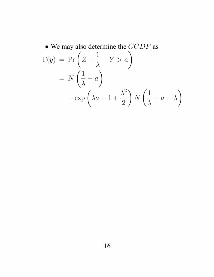
•We may also determine the CCDF as

Γ(y) = Pr

µZ +

1

λ− Y > a

¶= N

µ1

λ− a

¶− exp

µλa− 1 + λ2

2

¶N

µ1

λ− a− λ

¶

16

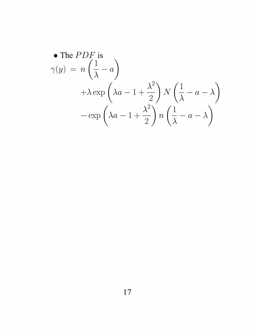
• The PDF is

γ(y) = n

µ1

λ− a

¶+λ exp

µλa− 1 + λ2

2

¶N

µ1

λ− a− λ

¶− exp

µλa− 1 + λ2

2

¶n

µ1

λ− a− λ

¶

17

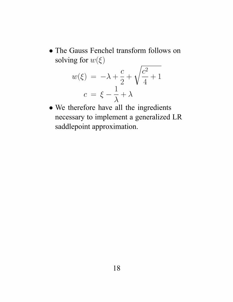
• The Gauss Fenchel transform follows onsolving for w(ξ)

w(ξ) = −λ+ c

2+

rc2

4+ 1

c = ξ − 1λ+ λ

•We therefore have all the ingredientsnecessary to implement a generalized LRsaddlepoint approximation.

18

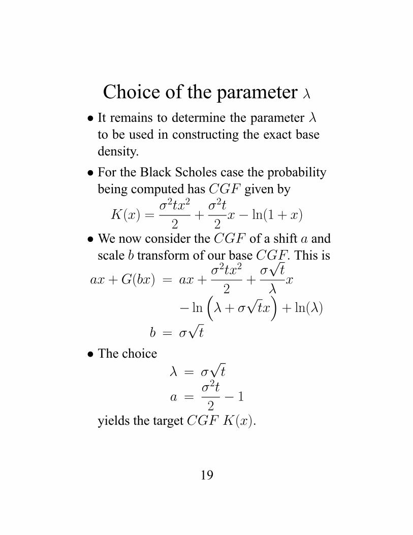
Choice of the parameter λ• It remains to determine the parameter λto be used in constructing the exact basedensity.

• For the Black Scholes case the probabilitybeing computed has CGF given by

K(x) =σ2tx2

2+σ2t

2x− ln(1 + x)

•We now consider the CGF of a shift a andscale b transform of our base CGF. This is

ax +G(bx) = ax +σ2tx2

2+σ√t

λx

− ln³λ+ σ

√tx´+ ln(λ)

b = σ√t

• The choiceλ = σ

√t

a =σ2t

2− 1

yields the target CGF K(x).

19

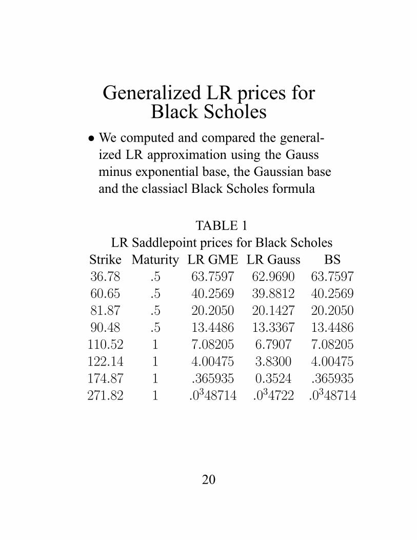
Generalized LR prices forBlack Scholes

•We computed and compared the general-ized LR approximation using the Gaussminus exponential base, the Gaussian baseand the classiacl Black Scholes formula

TABLE 1LR Saddlepoint prices for Black Scholes

Strike Maturity LR GME LR Gauss BS36.78 .5 63.7597 62.9690 63.759760.65 .5 40.2569 39.8812 40.256981.87 .5 20.2050 20.1427 20.205090.48 .5 13.4486 13.3367 13.4486110.52 1 7.08205 6.7907 7.08205122.14 1 4.00475 3.8300 4.00475174.87 1 .365935 0.3524 .365935271.82 1 .0348714 .034722 .0348714

20

•A General PurposeSaddlepoint Pricer

•We then moved on to construct a generalpurpose saddlepoint pricer that takes asinput the CGF of the logarithm of thestock price and its first two derivatives.

• The general choice of λ is given byλ = [K 00(bt + 1)]1/2.

• The pricer takes as inputs a vector of spotprices, strikes, rates, div yields, maturities,and returns call prices for an arbitrarymodel with parameters in the vector xx.

• The name of the arbitrary model is anadditional input.

21

• The pricing was completed for the sixmodels

CGMY

CGY SN

V GSSD

SV J

HSV

V GSA

22

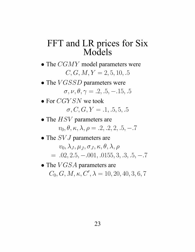
FFT and LR prices for SixModels

• The CGMY model parameters wereC,G,M, Y = 2, 5, 10, .5

• The V GSSD parameters wereσ, ν, θ, γ = .2, .5,−.15, .5

• For CGY SN we tookσ,C,G, Y = .1, .5, 5, .5

• TheHSV parameters arev0, θ, κ, λ, ρ = .2, .2, 2, .5,−.7

• The SV J parameters arev0, λJ, μJ, σJ, κ, θ, λ, ρ

= .02, 2.5,−.001, .0155, 3, .3, .5,−.7• The V GSA parameters are

C0, G,M, κ,C 0, λ = 10, 20, 40, 3, 6, 7

23

Conclusion• Saddlepoint methods classically computetail probabilities

•We show that call prices in log strike aretail probabilities that log stock prices underthe share measure exceed the log strike byan independent exponential variable

• In the Black Scholes this motivates theuse of a non-Gaussian base for an LRapproximation

• The base density is the law of a standardGaussian variate less an exponential withparameter λ.

24

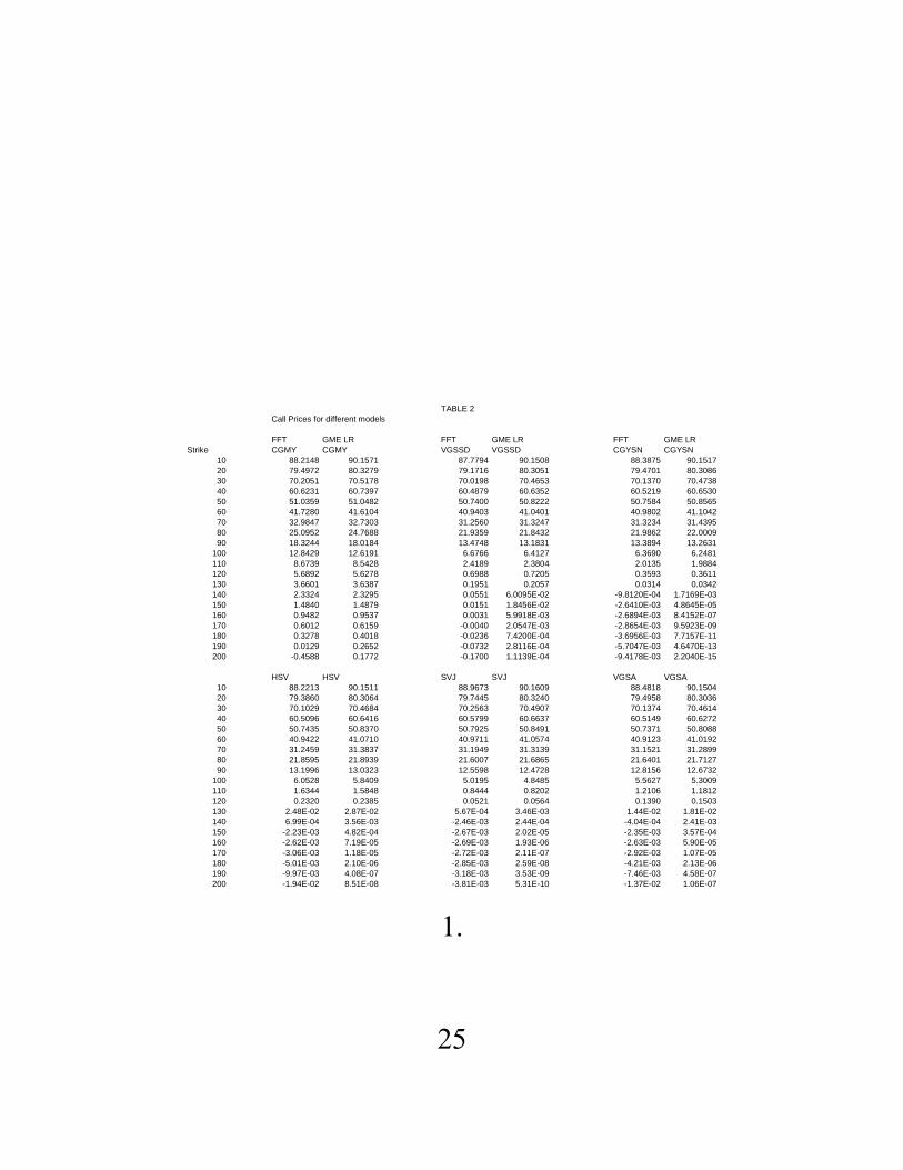
TABLE 2Call Prices for different models

FFT GME LR FFT GME LR FFT GME LRStrike CGMY CGMY VGSSD VGSSD CGYSN CGYSN

10 88.2148 90.1571 87.7794 90.1508 88.3875 90.151720 79.4972 80.3279 79.1716 80.3051 79.4701 80.308630 70.2051 70.5178 70.0198 70.4653 70.1370 70.473840 60.6231 60.7397 60.4879 60.6352 60.5219 60.653050 51.0359 51.0482 50.7400 50.8222 50.7584 50.856560 41.7280 41.6104 40.9403 41.0401 40.9802 41.104270 32.9847 32.7303 31.2560 31.3247 31.3234 31.439580 25.0952 24.7688 21.9359 21.8432 21.9862 22.000990 18.3244 18.0184 13.4748 13.1831 13.3894 13.2631

100 12.8429 12.6191 6.6766 6.4127 6.3690 6.2481110 8.6739 8.5428 2.4189 2.3804 2.0135 1.9884120 5.6892 5.6278 0.6988 0.7205 0.3593 0.3611130 3.6601 3.6387 0.1951 0.2057 0.0314 0.0342140 2.3324 2.3295 0.0551 6.0095E-02 -9.8120E-04 1.7169E-03150 1.4840 1.4879 0.0151 1.8456E-02 -2.6410E-03 4.8645E-05160 0.9482 0.9537 0.0031 5.9918E-03 -2.6894E-03 8.4152E-07170 0.6012 0.6159 -0.0040 2.0547E-03 -2.8654E-03 9.5923E-09180 0.3278 0.4018 -0.0236 7.4200E-04 -3.6956E-03 7.7157E-11190 0.0129 0.2652 -0.0732 2.8116E-04 -5.7047E-03 4.6470E-13200 -0.4588 0.1772 -0.1700 1.1139E-04 -9.4178E-03 2.2040E-15

HSV HSV SVJ SVJ VGSA VGSA10 88.2213 90.1511 88.9673 90.1609 88.4818 90.150420 79.3860 80.3064 79.7445 80.3240 79.4958 80.303630 70.1029 70.4684 70.2563 70.4907 70.1374 70.461440 60.5096 60.6416 60.5799 60.6637 60.5149 60.627250 50.7435 50.8370 50.7925 50.8491 50.7371 50.808860 40.9422 41.0710 40.9711 41.0574 40.9123 41.019270 31.2459 31.3837 31.1949 31.3139 31.1521 31.289980 21.8595 21.8939 21.6007 21.6865 21.6401 21.712790 13.1996 13.0323 12.5598 12.4728 12.8156 12.6732

100 6.0528 5.8409 5.0195 4.8485 5.5627 5.3009110 1.6344 1.5848 0.8444 0.8202 1.2106 1.1812120 0.2320 0.2385 0.0521 0.0564 0.1390 0.1503130 2.48E-02 2.87E-02 5.67E-04 3.46E-03 1.44E-02 1.81E-02140 6.99E-04 3.56E-03 -2.46E-03 2.44E-04 -4.04E-04 2.41E-03150 -2.23E-03 4.82E-04 -2.67E-03 2.02E-05 -2.35E-03 3.57E-04160 -2.62E-03 7.19E-05 -2.69E-03 1.93E-06 -2.63E-03 5.90E-05170 -3.06E-03 1.18E-05 -2.72E-03 2.11E-07 -2.92E-03 1.07E-05180 -5.01E-03 2.10E-06 -2.85E-03 2.59E-08 -4.21E-03 2.13E-06190 -9.97E-03 4.08E-07 -3.18E-03 3.53E-09 -7.46E-03 4.58E-07200 -1.94E-02 8.51E-08 -3.81E-03 5.31E-10 -1.37E-02 1.06E-07

1.

25

• It is observed theoretically and computa-tionally that this base is exact for the BlackScholes call price as a tail probability.

• This base is then used to develop a generalsaddlepoint pricer

• The general pricer is applied to six modelsand it is shown that the resulting saddle-point prices work effectively for out ofthe money options where Fourier methodsoften give negative prices.

26