MA 106 Linear Algebra - IIT Bombay
236
Elementary Matrices Consider a m × m matrix E ij whose (i , j ) th entry is 1 and all other entries are 0. 21/45
Transcript of MA 106 Linear Algebra - IIT Bombay

Elementary Matrices
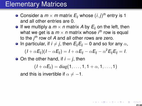
Consider a m ×m matrix Eij whose (i , j)th entry is 1and all other entries are 0.
If we multiply a m × n matrix A by Eij on the left, thenwhat we get is a m × n matrix whose i th row is equalto the j th row of A and all other rows are zero.In particular, if i 6= j , then EijEij = 0 and so for any α,
(I + αEij)(I − αEij) = I + αEij − αEij − α2EijEij = I.
On the other hand, if i = j , then
(I + αEii) = diag(1, . . . ,1,1 + α, 1, . . . ,1)
and this is invertible if α 6= −1.Matrices of the type I + αEij , with α ∈ R and i 6= j orof the type I + αEii with α 6= −1 provide simpleexamples of invertible matrices whose inverse is of asimilar type. These are two among 3 possible typesof elementary matrices.
21/45

Elementary Matrices
Consider a m ×m matrix Eij whose (i , j)th entry is 1and all other entries are 0.If we multiply a m × n matrix A by Eij on the left, thenwhat we get is a m × n matrix whose i th row is equalto the j th row of A and all other rows are zero.
In particular, if i 6= j , then EijEij = 0 and so for any α,
(I + αEij)(I − αEij) = I + αEij − αEij − α2EijEij = I.
On the other hand, if i = j , then
(I + αEii) = diag(1, . . . ,1,1 + α, 1, . . . ,1)
and this is invertible if α 6= −1.Matrices of the type I + αEij , with α ∈ R and i 6= j orof the type I + αEii with α 6= −1 provide simpleexamples of invertible matrices whose inverse is of asimilar type. These are two among 3 possible typesof elementary matrices.
21/45

Elementary Matrices
Consider a m ×m matrix Eij whose (i , j)th entry is 1and all other entries are 0.If we multiply a m × n matrix A by Eij on the left, thenwhat we get is a m × n matrix whose i th row is equalto the j th row of A and all other rows are zero.In particular, if i 6= j , then EijEij = 0 and so for any α,
(I + αEij)(I − αEij) = I + αEij − αEij − α2EijEij = I.
On the other hand, if i = j , then
(I + αEii) = diag(1, . . . ,1,1 + α, 1, . . . ,1)
and this is invertible if α 6= −1.Matrices of the type I + αEij , with α ∈ R and i 6= j orof the type I + αEii with α 6= −1 provide simpleexamples of invertible matrices whose inverse is of asimilar type. These are two among 3 possible typesof elementary matrices.
21/45
Elementary Matrices
Consider a m ×m matrix Eij whose (i , j)th entry is 1and all other entries are 0.If we multiply a m × n matrix A by Eij on the left, thenwhat we get is a m × n matrix whose i th row is equalto the j th row of A and all other rows are zero.In particular, if i 6= j , then EijEij = 0 and so for any α,
(I + αEij)(I − αEij) = I + αEij − αEij − α2EijEij = I.
On the other hand, if i = j , then
(I + αEii) = diag(1, . . . ,1,1 + α, 1, . . . ,1)
and this is invertible if α 6= −1.
Matrices of the type I + αEij , with α ∈ R and i 6= j orof the type I + αEii with α 6= −1 provide simpleexamples of invertible matrices whose inverse is of asimilar type. These are two among 3 possible typesof elementary matrices.
21/45

Elementary Matrices
Consider a m ×m matrix Eij whose (i , j)th entry is 1and all other entries are 0.If we multiply a m × n matrix A by Eij on the left, thenwhat we get is a m × n matrix whose i th row is equalto the j th row of A and all other rows are zero.In particular, if i 6= j , then EijEij = 0 and so for any α,
(I + αEij)(I − αEij) = I + αEij − αEij − α2EijEij = I.
On the other hand, if i = j , then
(I + αEii) = diag(1, . . . ,1,1 + α, 1, . . . ,1)
and this is invertible if α 6= −1.Matrices of the type I + αEij , with α ∈ R and i 6= j orof the type I + αEii with α 6= −1 provide simpleexamples of invertible matrices whose inverse is of asimilar type. These are two among 3 possible typesof elementary matrices.
21/45
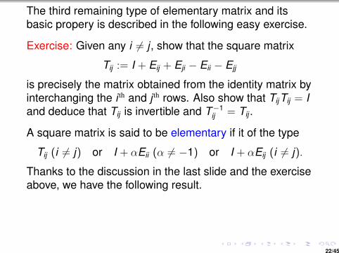
The third remaining type of elementary matrix and itsbasic propery is described in the following easy exercise.
Exercise: Given any i 6= j , show that the square matrix
Tij := I + Eij + Eji − Eii − Ejj
is precisely the matrix obtained from the identity matrix byinterchanging the i th and j th rows. Also show that TijTij = Iand deduce that Tij is invertible and T−1
ij = Tij .
A square matrix is said to be elementary if it of the type
Tij (i 6= j) or I + αEii (α 6= −1) or I + αEij (i 6= j).
Thanks to the discussion in the last slide and the exerciseabove, we have the following result.
TheoremEvery elementary matrix is invertible and its inverse is anelementary matrix of the same type.
22/45

Permutation Matrices
Let n be a positive integer. A permutation of1,2, . . . ,n is a one-one and onto mapping of the set{1,2, . . . ,n} onto itself.
Associated to a permutation σ of {1,2, . . . ,n}, wedefine a n × n matrix Pσ = (pij) as follows.
pij =
{0 if i 6= σ(j)1 if i = σ(j)
This is called a permutation matrix assoicated to σ.A permutation matrix is obtained by shuffling the rowsof the identity matrix (or by shuffling the columns).If A is a permutation matrix, then
AAT = AT A = In.
In particular, permutation matrices are invertible.
23/45

Permutation Matrices
Let n be a positive integer. A permutation of1,2, . . . ,n is a one-one and onto mapping of the set{1,2, . . . ,n} onto itself.Associated to a permutation σ of {1,2, . . . ,n}, wedefine a n × n matrix Pσ = (pij) as follows.
pij =
{0 if i 6= σ(j)1 if i = σ(j)
This is called a permutation matrix assoicated to σ.
A permutation matrix is obtained by shuffling the rowsof the identity matrix (or by shuffling the columns).If A is a permutation matrix, then
AAT = AT A = In.
In particular, permutation matrices are invertible.
23/45

Permutation Matrices
Let n be a positive integer. A permutation of1,2, . . . ,n is a one-one and onto mapping of the set{1,2, . . . ,n} onto itself.Associated to a permutation σ of {1,2, . . . ,n}, wedefine a n × n matrix Pσ = (pij) as follows.
pij =
{0 if i 6= σ(j)1 if i = σ(j)
This is called a permutation matrix assoicated to σ.A permutation matrix is obtained by shuffling the rowsof the identity matrix (or by shuffling the columns).
If A is a permutation matrix, then
AAT = AT A = In.
In particular, permutation matrices are invertible.
23/45

Permutation Matrices
Let n be a positive integer. A permutation of1,2, . . . ,n is a one-one and onto mapping of the set{1,2, . . . ,n} onto itself.Associated to a permutation σ of {1,2, . . . ,n}, wedefine a n × n matrix Pσ = (pij) as follows.
pij =
{0 if i 6= σ(j)1 if i = σ(j)
This is called a permutation matrix assoicated to σ.A permutation matrix is obtained by shuffling the rowsof the identity matrix (or by shuffling the columns).If A is a permutation matrix, then
AAT = AT A = In.
In particular, permutation matrices are invertible.23/45
Gaussian Elimination
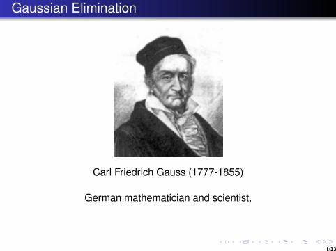
Carl Friedrich Gauss (1777-1855)
German mathematician and scientist,
contributed to number theory, statistics, algebra, analysis,differential geometry, geophysics, electrostatics, astronomy,
optics
1/33

Gaussian Elimination
Carl Friedrich Gauss (1777-1855)
German mathematician and scientist,contributed to number theory, statistics, algebra, analysis,
differential geometry, geophysics, electrostatics, astronomy,optics
1/33
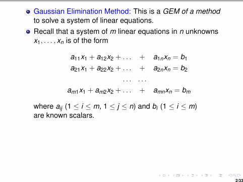
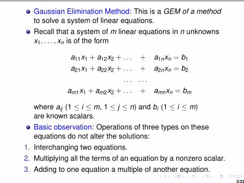
Gaussian Elimination Method: This is a GEM of a methodto solve a system of linear equations.
Recall that a system of m linear equations in n unknownsx1, . . . , xn is of the form
a11x1 + a12x2 + . . . + a1nxn = b1
a21x1 + a22x2 + . . . + a2nxn = b2
. . . . . .
am1x1 + am2x2 + . . . + amnxn = bm
where aij (1 ≤ i ≤ m, 1 ≤ j ≤ n) and bi (1 ≤ i ≤ m)are known scalars.
Basic observation: Operations of three types on theseequations do not alter the solutions:
1. Interchanging two equations.2. Multiplying all the terms of an equation by a nonzero scalar.3. Adding to one equation a multiple of another equation.
2/33
Gaussian Elimination Method: This is a GEM of a methodto solve a system of linear equations.Recall that a system of m linear equations in n unknownsx1, . . . , xn is of the form
a11x1 + a12x2 + . . . + a1nxn = b1
a21x1 + a22x2 + . . . + a2nxn = b2
. . . . . .
am1x1 + am2x2 + . . . + amnxn = bm
where aij (1 ≤ i ≤ m, 1 ≤ j ≤ n) and bi (1 ≤ i ≤ m)are known scalars.
Basic observation: Operations of three types on theseequations do not alter the solutions:
1. Interchanging two equations.2. Multiplying all the terms of an equation by a nonzero scalar.3. Adding to one equation a multiple of another equation.
2/33

Gaussian Elimination Method: This is a GEM of a methodto solve a system of linear equations.Recall that a system of m linear equations in n unknownsx1, . . . , xn is of the form
a11x1 + a12x2 + . . . + a1nxn = b1
a21x1 + a22x2 + . . . + a2nxn = b2
. . . . . .
am1x1 + am2x2 + . . . + amnxn = bm
where aij (1 ≤ i ≤ m, 1 ≤ j ≤ n) and bi (1 ≤ i ≤ m)are known scalars.Basic observation: Operations of three types on theseequations do not alter the solutions:
1. Interchanging two equations.
2. Multiplying all the terms of an equation by a nonzero scalar.3. Adding to one equation a multiple of another equation.
2/33

Gaussian Elimination Method: This is a GEM of a methodto solve a system of linear equations.Recall that a system of m linear equations in n unknownsx1, . . . , xn is of the form
a11x1 + a12x2 + . . . + a1nxn = b1
a21x1 + a22x2 + . . . + a2nxn = b2
. . . . . .
am1x1 + am2x2 + . . . + amnxn = bm
where aij (1 ≤ i ≤ m, 1 ≤ j ≤ n) and bi (1 ≤ i ≤ m)are known scalars.Basic observation: Operations of three types on theseequations do not alter the solutions:
1. Interchanging two equations.2. Multiplying all the terms of an equation by a nonzero scalar.
3. Adding to one equation a multiple of another equation.
2/33
Gaussian Elimination Method: This is a GEM of a methodto solve a system of linear equations.Recall that a system of m linear equations in n unknownsx1, . . . , xn is of the form
a11x1 + a12x2 + . . . + a1nxn = b1
a21x1 + a22x2 + . . . + a2nxn = b2
. . . . . .
am1x1 + am2x2 + . . . + amnxn = bm
where aij (1 ≤ i ≤ m, 1 ≤ j ≤ n) and bi (1 ≤ i ≤ m)are known scalars.Basic observation: Operations of three types on theseequations do not alter the solutions:
1. Interchanging two equations.2. Multiplying all the terms of an equation by a nonzero scalar.3. Adding to one equation a multiple of another equation.
2/33

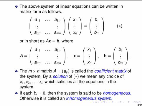
The above system of linear equations can be written inmatrix form as follows. a11 . . . a1n
......
am1 . . . amn
x1
...xn
=
b1...
bm
(∗)
or in short as Ax = b, where
A =
a11 . . . a1n...
...am1 . . . amn
, x =
x1...
xn
, b =
b1...
bm
.
The m× n matrix A = (aij) is called the coefficient matrix ofthe system. By a solution of (∗) we mean any choice ofx1, x2, . . . , xn which satisfies all the equations in thesystem.If each bi = 0, then the system is said to be homogeneous.Otherwise it is called an inhomogeneous system.
3/33

The above system of linear equations can be written inmatrix form as follows. a11 . . . a1n
......
am1 . . . amn
x1
...xn
=
b1...
bm
(∗)
or in short as Ax = b, where
A =
a11 . . . a1n...
...am1 . . . amn
, x =
x1...
xn
, b =
b1...
bm
.
The m× n matrix A = (aij) is called the coefficient matrix ofthe system. By a solution of (∗) we mean any choice ofx1, x2, . . . , xn which satisfies all the equations in thesystem.
If each bi = 0, then the system is said to be homogeneous.Otherwise it is called an inhomogeneous system.
3/33
The above system of linear equations can be written inmatrix form as follows. a11 . . . a1n
......
am1 . . . amn
x1
...xn
=
b1...
bm
(∗)
or in short as Ax = b, where
A =
a11 . . . a1n...
...am1 . . . amn
, x =
x1...
xn
, b =
b1...
bm
.
The m× n matrix A = (aij) is called the coefficient matrix ofthe system. By a solution of (∗) we mean any choice ofx1, x2, . . . , xn which satisfies all the equations in thesystem.If each bi = 0, then the system is said to be homogeneous.Otherwise it is called an inhomogeneous system.
3/33

All the known data in the system (∗) is captured in them × (n + 1) matrix
(A|b) :=
a11 . . . a1n...
...am1 . . . amn
∣∣∣∣∣∣∣b1...
bm
.
This is called the augmented matrix for the system.
Now the above three operations on the equations in thelinear system correspond to the following operations on therows of the augmented matrix:
(i) interchanging two rows,(ii) multiply a row by a nonzero scalar,(iii) adding a multiple of one row to another.
These are called elementary row operations.
Gaussian Elimination Method consists of reducing theaugmented matrix to a simpler matrix from which solutionscan be easily found. This reduction is by means ofelementary row operations.
4/33

All the known data in the system (∗) is captured in them × (n + 1) matrix
(A|b) :=
a11 . . . a1n...
...am1 . . . amn
∣∣∣∣∣∣∣b1...
bm
.
This is called the augmented matrix for the system.Now the above three operations on the equations in thelinear system correspond to the following operations on therows of the augmented matrix:
(i) interchanging two rows,(ii) multiply a row by a nonzero scalar,(iii) adding a multiple of one row to another.
These are called elementary row operations.
Gaussian Elimination Method consists of reducing theaugmented matrix to a simpler matrix from which solutionscan be easily found. This reduction is by means ofelementary row operations.
4/33

Example 1 (A system with a unique solution):
x − 2y + z = 52x − 5y + 4z = −3
x − 4y + 6z = 10.
The augmented matrix for this system is the 3× 4 matrix 1 −2 12 −5 41 −4 6
∣∣∣∣∣∣5−310
The elementary row operations mentioned above will beperformed on the rows of this augmented matrix,
5/33

Example 1 (A system with a unique solution):
x − 2y + z = 52x − 5y + 4z = −3
x − 4y + 6z = 10.
The augmented matrix for this system is the 3× 4 matrix 1 −2 12 −5 41 −4 6
∣∣∣∣∣∣5−310
The elementary row operations mentioned above will beperformed on the rows of this augmented matrix,
5/33

First we add -2 times the first row to the second row. Then wesubtract the first row from the third row.
i.e.,
1 −2 10 −1 20 −2 5
∣∣∣∣∣∣5−13
5
The circled entry is the first nonzero entry in the first rowand all the entries below this are 0. Such a circled entry iscalled a pivot. This next step is called ‘sweeping’ a column.Here we repeat the process for the smaller matrix:
viz.(−1 2−2 5
∣∣∣∣ −135
)⇒
(-1 2
0 1
∣∣∣∣∣ −1331
)Put back the rows and columns that has been cut outearlier:
6/33

First we add -2 times the first row to the second row. Then wesubtract the first row from the third row.
i.e.,
1 −2 10 −1 20 −2 5
∣∣∣∣∣∣5−13
5
The circled entry is the first nonzero entry in the first rowand all the entries below this are 0. Such a circled entry iscalled a pivot. This next step is called ‘sweeping’ a column.Here we repeat the process for the smaller matrix:
viz.(−1 2−2 5
∣∣∣∣ −135
)
⇒
(-1 2
0 1
∣∣∣∣∣ −1331
)Put back the rows and columns that has been cut outearlier:
6/33

First we add -2 times the first row to the second row. Then wesubtract the first row from the third row.
i.e.,
1 −2 10 −1 20 −2 5
∣∣∣∣∣∣5−13
5
The circled entry is the first nonzero entry in the first rowand all the entries below this are 0. Such a circled entry iscalled a pivot. This next step is called ‘sweeping’ a column.Here we repeat the process for the smaller matrix:
viz.(−1 2−2 5
∣∣∣∣ −135
)⇒
(-1 2
0 1
∣∣∣∣∣ −1331
)
Put back the rows and columns that has been cut outearlier:
6/33

First we add -2 times the first row to the second row. Then wesubtract the first row from the third row.
i.e.,
1 −2 10 −1 20 −2 5
∣∣∣∣∣∣5−13
5
The circled entry is the first nonzero entry in the first rowand all the entries below this are 0. Such a circled entry iscalled a pivot. This next step is called ‘sweeping’ a column.Here we repeat the process for the smaller matrix:
viz.(−1 2−2 5
∣∣∣∣ −135
)⇒
(-1 2
0 1
∣∣∣∣∣ −1331
)Put back the rows and columns that has been cut outearlier:
6/33

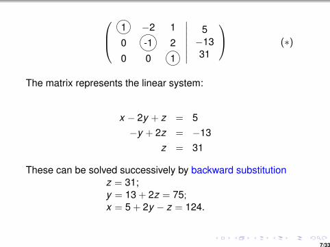
1 −2 1
0 -1 2
0 0 1
∣∣∣∣∣∣∣5−1331
(∗)
The matrix represents the linear system:
x − 2y + z = 5−y + 2z = −13
z = 31
These can be solved successively by backward substitutionz = 31;y = 13 + 2z = 75;x = 5 + 2y − z = 124.
7/33

1 −2 1
0 -1 2
0 0 1
∣∣∣∣∣∣∣5−1331
(∗)
The matrix represents the linear system:
x − 2y + z = 5−y + 2z = −13
z = 31
These can be solved successively by backward substitutionz = 31;y = 13 + 2z = 75;x = 5 + 2y − z = 124.
7/33

1 −2 1
0 -1 2
0 0 1
∣∣∣∣∣∣∣5−1331
(∗)
The matrix represents the linear system:
x − 2y + z = 5−y + 2z = −13
z = 31
These can be solved successively by backward substitutionz = 31;
y = 13 + 2z = 75;x = 5 + 2y − z = 124.
7/33

1 −2 1
0 -1 2
0 0 1
∣∣∣∣∣∣∣5−1331
(∗)
The matrix represents the linear system:
x − 2y + z = 5−y + 2z = −13
z = 31
These can be solved successively by backward substitutionz = 31;y = 13 + 2z = 75;
x = 5 + 2y − z = 124.
7/33
1 −2 1
0 -1 2
0 0 1
∣∣∣∣∣∣∣5−1331
(∗)
The matrix represents the linear system:
x − 2y + z = 5−y + 2z = −13
z = 31
These can be solved successively by backward substitutionz = 31;y = 13 + 2z = 75;x = 5 + 2y − z = 124.
7/33

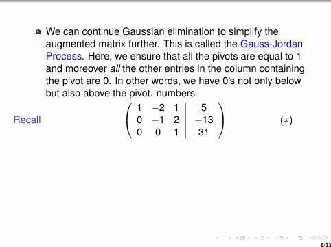
We can continue Gaussian elimination to simplify theaugmented matrix further. This is called the Gauss-JordanProcess.
Here, we ensure that all the pivots are equal to 1and moreover all the other entries in the column containingthe pivot are 0. In other words, we have 0’s not only belowbut also above the pivot. numbers.
Recall
1 −2 10 −1 20 0 1
∣∣∣∣∣∣5−1331
(∗)
(1) multiply the second row throughout by −1,(2) add twice third row to the second(3) then subtract the third row from the first(3) add twice the second row to the first
This gives
8/33

We can continue Gaussian elimination to simplify theaugmented matrix further. This is called the Gauss-JordanProcess. Here, we ensure that all the pivots are equal to 1and moreover all the other entries in the column containingthe pivot are 0. In other words, we have 0’s not only belowbut also above the pivot. numbers.
Recall
1 −2 10 −1 20 0 1
∣∣∣∣∣∣5−1331
(∗)
(1) multiply the second row throughout by −1,(2) add twice third row to the second(3) then subtract the third row from the first(3) add twice the second row to the first
This gives
8/33
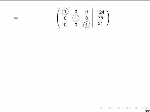
⇒
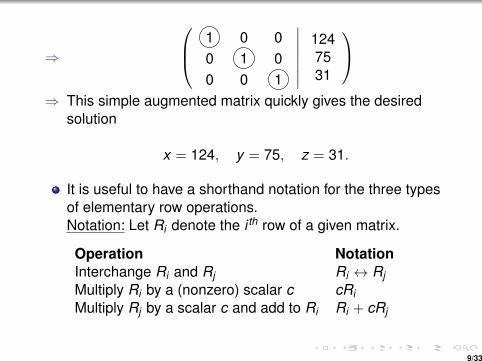
1 0 00 1 00 0 1
∣∣∣∣∣∣∣1247531
⇒ This simple augmented matrix quickly gives the desiredsolution
x = 124, y = 75, z = 31.
It is useful to have a shorthand notation for the three typesof elementary row operations.Notation: Let Ri denote the i th row of a given matrix.
Operation NotationInterchange Ri and Rj Ri ↔ RjMultiply Ri by a (nonzero) scalar c cRiMultiply Rj by a scalar c and add to Ri Ri + cRj
9/33

⇒
1 0 00 1 00 0 1
∣∣∣∣∣∣∣1247531
⇒ This simple augmented matrix quickly gives the desired
solution
x = 124, y = 75, z = 31.
It is useful to have a shorthand notation for the three typesof elementary row operations.Notation: Let Ri denote the i th row of a given matrix.
Operation NotationInterchange Ri and Rj Ri ↔ RjMultiply Ri by a (nonzero) scalar c cRiMultiply Rj by a scalar c and add to Ri Ri + cRj
9/33

Example 2 (A system with infinitely many solutions):
x − 2y + z − u + v = 52x − 5y + 4z + u − v = −3x − 4y + 6z + 2u − v = 10
⇒
1 −2 1 −1 12 −5 4 1 −11 −4 6 2 −1
∣∣∣∣∣∣5−310
We shall use the notation introduced above for the rowoperations
.R2 − 2R1R3 − R1−→
1 −2 1 −1 10 −1 2 3 −30 −2 5 3 −2
∣∣∣∣∣∣5−13
5
.
R3 − 2R2−→
1 −2 1 −1 10 −1 2 3 −30 0 1 −3 4
∣∣∣∣∣∣5−1331
10/33

Example 2 (A system with infinitely many solutions):
x − 2y + z − u + v = 52x − 5y + 4z + u − v = −3x − 4y + 6z + 2u − v = 10
⇒
1 −2 1 −1 12 −5 4 1 −11 −4 6 2 −1
∣∣∣∣∣∣5−310
We shall use the notation introduced above for the rowoperations
.R2 − 2R1R3 − R1−→
1 −2 1 −1 10 −1 2 3 −30 −2 5 3 −2
∣∣∣∣∣∣5−13
5
.R3 − 2R2−→
1 −2 1 −1 10 −1 2 3 −30 0 1 −3 4
∣∣∣∣∣∣5−1331
10/33

Example 2 (A system with infinitely many solutions):
x − 2y + z − u + v = 52x − 5y + 4z + u − v = −3x − 4y + 6z + 2u − v = 10
⇒
1 −2 1 −1 12 −5 4 1 −11 −4 6 2 −1
∣∣∣∣∣∣5−310
We shall use the notation introduced above for the rowoperations
.R2 − 2R1R3 − R1−→
1 −2 1 −1 10 −1 2 3 −30 −2 5 3 −2
∣∣∣∣∣∣5−13
5
.
R3 − 2R2−→
1 −2 1 −1 10 −1 2 3 −30 0 1 −3 4
∣∣∣∣∣∣5−1331
10/33

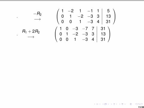
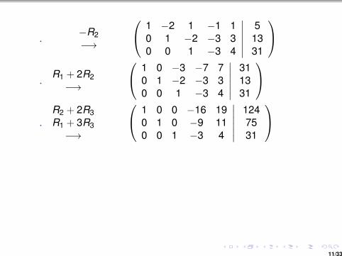
.−R2−→
1 −2 1 −1 10 1 −2 −3 30 0 1 −3 4
∣∣∣∣∣∣51331
.R1 + 2R2−→
1 0 −3 −7 70 1 −2 −3 30 0 1 −3 4
∣∣∣∣∣∣311331
.
R2 + 2R3R1 + 3R3−→
1 0 0 −16 190 1 0 −9 110 0 1 −3 4
∣∣∣∣∣∣1247531
The system of linear equations corresponding to the lastaugmented matrix is:
x = 124 + 16u − 19vy = 75 + 9u − 11vz = 31 + 3u − 4v .
11/33
.−R2−→
1 −2 1 −1 10 1 −2 −3 30 0 1 −3 4
∣∣∣∣∣∣51331
.
R1 + 2R2−→
1 0 −3 −7 70 1 −2 −3 30 0 1 −3 4
∣∣∣∣∣∣311331
.R2 + 2R3R1 + 3R3−→
1 0 0 −16 190 1 0 −9 110 0 1 −3 4
∣∣∣∣∣∣1247531
The system of linear equations corresponding to the lastaugmented matrix is:
x = 124 + 16u − 19vy = 75 + 9u − 11vz = 31 + 3u − 4v .
11/33
.−R2−→
1 −2 1 −1 10 1 −2 −3 30 0 1 −3 4
∣∣∣∣∣∣51331
.
R1 + 2R2−→
1 0 −3 −7 70 1 −2 −3 30 0 1 −3 4
∣∣∣∣∣∣311331
.
R2 + 2R3R1 + 3R3−→
1 0 0 −16 190 1 0 −9 110 0 1 −3 4
∣∣∣∣∣∣1247531
The system of linear equations corresponding to the lastaugmented matrix is:
x = 124 + 16u − 19vy = 75 + 9u − 11vz = 31 + 3u − 4v .
11/33

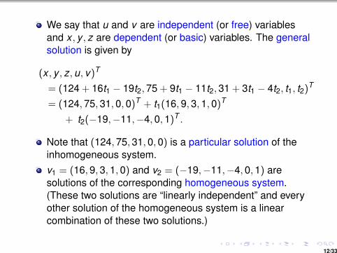
We say that u and v are independent (or free) variablesand x , y , z are dependent (or basic) variables. The generalsolution is given by
(x , y , z,u, v)T
= (124 + 16t1 − 19t2,75 + 9t1 − 11t2,31 + 3t1 − 4t2, t1, t2)T
= (124,75,31,0,0)T + t1(16,9,3,1,0)T
+ t2(−19,−11,−4,0,1)T .
Note that (124,75,31,0,0) is a particular solution of theinhomogeneous system.v1 = (16,9,3,1,0) and v2 = (−19,−11,−4,0,1) aresolutions of the corresponding homogeneous system.(These two solutions are “linearly independent” and everyother solution of the homogeneous system is a linearcombination of these two solutions.)
12/33

We say that u and v are independent (or free) variablesand x , y , z are dependent (or basic) variables. The generalsolution is given by
(x , y , z,u, v)T
= (124 + 16t1 − 19t2,75 + 9t1 − 11t2,31 + 3t1 − 4t2, t1, t2)T
= (124,75,31,0,0)T + t1(16,9,3,1,0)T
+ t2(−19,−11,−4,0,1)T .
Note that (124,75,31,0,0) is a particular solution of theinhomogeneous system.
v1 = (16,9,3,1,0) and v2 = (−19,−11,−4,0,1) aresolutions of the corresponding homogeneous system.(These two solutions are “linearly independent” and everyother solution of the homogeneous system is a linearcombination of these two solutions.)
12/33

We say that u and v are independent (or free) variablesand x , y , z are dependent (or basic) variables. The generalsolution is given by
(x , y , z,u, v)T
= (124 + 16t1 − 19t2,75 + 9t1 − 11t2,31 + 3t1 − 4t2, t1, t2)T
= (124,75,31,0,0)T + t1(16,9,3,1,0)T
+ t2(−19,−11,−4,0,1)T .
Note that (124,75,31,0,0) is a particular solution of theinhomogeneous system.v1 = (16,9,3,1,0) and v2 = (−19,−11,−4,0,1) aresolutions of the corresponding homogeneous system.
(These two solutions are “linearly independent” and everyother solution of the homogeneous system is a linearcombination of these two solutions.)
12/33
We say that u and v are independent (or free) variablesand x , y , z are dependent (or basic) variables. The generalsolution is given by
(x , y , z,u, v)T
= (124 + 16t1 − 19t2,75 + 9t1 − 11t2,31 + 3t1 − 4t2, t1, t2)T
= (124,75,31,0,0)T + t1(16,9,3,1,0)T
+ t2(−19,−11,−4,0,1)T .
Note that (124,75,31,0,0) is a particular solution of theinhomogeneous system.v1 = (16,9,3,1,0) and v2 = (−19,−11,−4,0,1) aresolutions of the corresponding homogeneous system.(These two solutions are “linearly independent” and everyother solution of the homogeneous system is a linearcombination of these two solutions.)
12/33
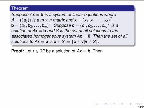
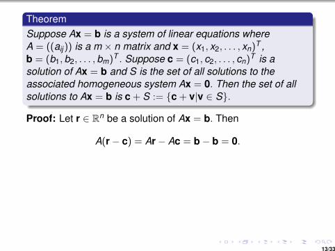
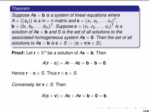
TheoremSuppose Ax = b is a system of linear equations whereA = ((aij)) is a m × n matrix and x = (x1, x2, . . . , xn)
T ,b = (b1,b2, . . . ,bm)
T .
Suppose c = (c1, c2, . . . , cn)T is a
solution of Ax = b and S is the set of all solutions to theassociated homogeneous system Ax = 0. Then the set of allsolutions to Ax = b is c + S := {c + v|v ∈ S}.
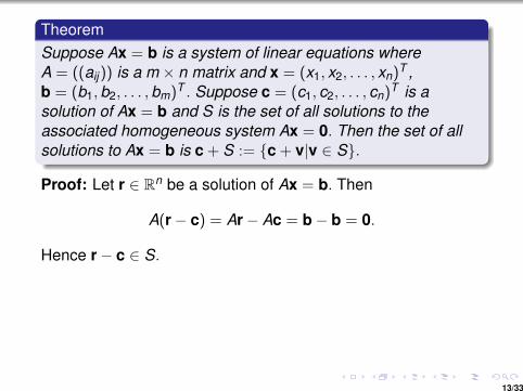
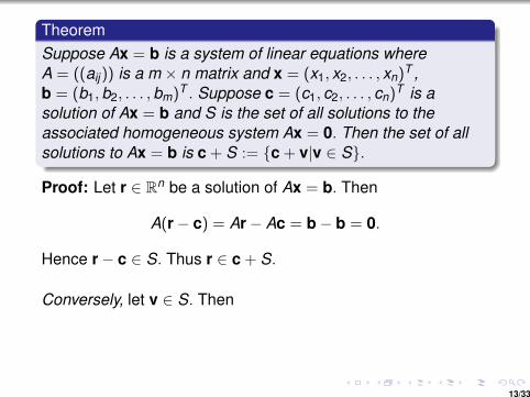
Proof: Let r ∈ Rn be a solution of Ax = b. Then
A(r− c) = Ar− Ac = b− b = 0.
Hence r− c ∈ S. Thus r ∈ c + S.
Conversely, let v ∈ S. Then
A(c + v) = Ac + Av = b + 0 = b.
Hence c + v is a solution to Ax = b. 2
13/33
TheoremSuppose Ax = b is a system of linear equations whereA = ((aij)) is a m × n matrix and x = (x1, x2, . . . , xn)
T ,b = (b1,b2, . . . ,bm)
T . Suppose c = (c1, c2, . . . , cn)T is a
solution of Ax = b and S is the set of all solutions to theassociated homogeneous system Ax = 0.
Then the set of allsolutions to Ax = b is c + S := {c + v|v ∈ S}.
Proof: Let r ∈ Rn be a solution of Ax = b. Then
A(r− c) = Ar− Ac = b− b = 0.
Hence r− c ∈ S. Thus r ∈ c + S.
Conversely, let v ∈ S. Then
A(c + v) = Ac + Av = b + 0 = b.
Hence c + v is a solution to Ax = b. 2
13/33

TheoremSuppose Ax = b is a system of linear equations whereA = ((aij)) is a m × n matrix and x = (x1, x2, . . . , xn)
T ,b = (b1,b2, . . . ,bm)
T . Suppose c = (c1, c2, . . . , cn)T is a
solution of Ax = b and S is the set of all solutions to theassociated homogeneous system Ax = 0. Then the set of allsolutions to Ax = b is c + S := {c + v|v ∈ S}.
Proof: Let r ∈ Rn be a solution of Ax = b. Then
A(r− c) = Ar− Ac = b− b = 0.
Hence r− c ∈ S. Thus r ∈ c + S.
Conversely, let v ∈ S. Then
A(c + v) = Ac + Av = b + 0 = b.
Hence c + v is a solution to Ax = b. 2
13/33
TheoremSuppose Ax = b is a system of linear equations whereA = ((aij)) is a m × n matrix and x = (x1, x2, . . . , xn)
T ,b = (b1,b2, . . . ,bm)
T . Suppose c = (c1, c2, . . . , cn)T is a
solution of Ax = b and S is the set of all solutions to theassociated homogeneous system Ax = 0. Then the set of allsolutions to Ax = b is c + S := {c + v|v ∈ S}.
Proof: Let r ∈ Rn be a solution of Ax = b. Then
A(r− c) = Ar− Ac = b− b = 0.
Hence r− c ∈ S.
Thus r ∈ c + S.
Conversely, let v ∈ S. Then
A(c + v) = Ac + Av = b + 0 = b.
Hence c + v is a solution to Ax = b. 2
13/33

TheoremSuppose Ax = b is a system of linear equations whereA = ((aij)) is a m × n matrix and x = (x1, x2, . . . , xn)
T ,b = (b1,b2, . . . ,bm)
T . Suppose c = (c1, c2, . . . , cn)T is a
solution of Ax = b and S is the set of all solutions to theassociated homogeneous system Ax = 0. Then the set of allsolutions to Ax = b is c + S := {c + v|v ∈ S}.
Proof: Let r ∈ Rn be a solution of Ax = b. Then
A(r− c) = Ar− Ac = b− b = 0.
Hence r− c ∈ S. Thus r ∈ c + S.
Conversely, let v ∈ S. Then
A(c + v) = Ac + Av = b + 0 = b.
Hence c + v is a solution to Ax = b. 2
13/33
TheoremSuppose Ax = b is a system of linear equations whereA = ((aij)) is a m × n matrix and x = (x1, x2, . . . , xn)
T ,b = (b1,b2, . . . ,bm)
T . Suppose c = (c1, c2, . . . , cn)T is a
solution of Ax = b and S is the set of all solutions to theassociated homogeneous system Ax = 0. Then the set of allsolutions to Ax = b is c + S := {c + v|v ∈ S}.
Proof: Let r ∈ Rn be a solution of Ax = b. Then
A(r− c) = Ar− Ac = b− b = 0.
Hence r− c ∈ S. Thus r ∈ c + S.
Conversely, let v ∈ S. Then
A(c + v) = Ac + Av = b + 0 = b.
Hence c + v is a solution to Ax = b. 2
13/33

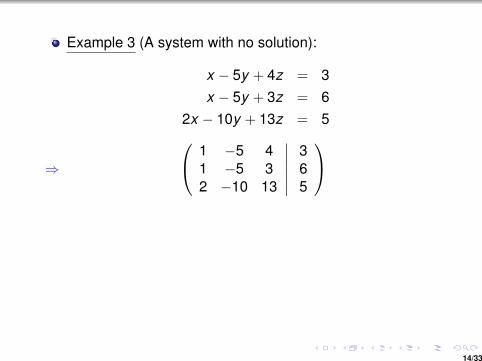
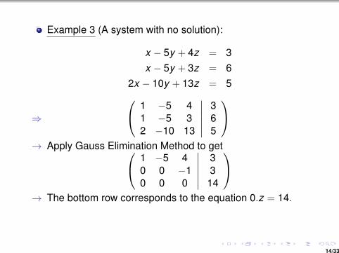
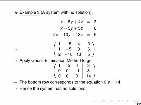
Example 3 (A system with no solution):
x − 5y + 4z = 3x − 5y + 3z = 6
2x − 10y + 13z = 5
⇒
1 −5 41 −5 32 −10 13
∣∣∣∣∣∣365
→ Apply Gauss Elimination Method to get 1 −5 4
0 0 −10 0 0
∣∣∣∣∣∣3314
→ The bottom row corresponds to the equation 0.z = 14.→ Hence the system has no solutions.
14/33
Example 3 (A system with no solution):
x − 5y + 4z = 3x − 5y + 3z = 6
2x − 10y + 13z = 5
⇒
1 −5 41 −5 32 −10 13
∣∣∣∣∣∣365
→ Apply Gauss Elimination Method to get 1 −5 40 0 −10 0 0
∣∣∣∣∣∣3314
→ The bottom row corresponds to the equation 0.z = 14.→ Hence the system has no solutions.
14/33

Example 3 (A system with no solution):
x − 5y + 4z = 3x − 5y + 3z = 6
2x − 10y + 13z = 5
⇒
1 −5 41 −5 32 −10 13
∣∣∣∣∣∣365
→ Apply Gauss Elimination Method to get 1 −5 4
0 0 −10 0 0
∣∣∣∣∣∣3314
→ The bottom row corresponds to the equation 0.z = 14.→ Hence the system has no solutions.
14/33
Example 3 (A system with no solution):
x − 5y + 4z = 3x − 5y + 3z = 6
2x − 10y + 13z = 5
⇒
1 −5 41 −5 32 −10 13
∣∣∣∣∣∣365
→ Apply Gauss Elimination Method to get 1 −5 4
0 0 −10 0 0
∣∣∣∣∣∣3314
→ The bottom row corresponds to the equation 0.z = 14.
→ Hence the system has no solutions.
14/33
Example 3 (A system with no solution):
x − 5y + 4z = 3x − 5y + 3z = 6
2x − 10y + 13z = 5
⇒
1 −5 41 −5 32 −10 13
∣∣∣∣∣∣365
→ Apply Gauss Elimination Method to get 1 −5 4
0 0 −10 0 0
∣∣∣∣∣∣3314
→ The bottom row corresponds to the equation 0.z = 14.→ Hence the system has no solutions.
14/33

STEPS IN GAUSSIAN ELIMINATIONStage 1: Forward Elimination Phase
The basic idea is to reduce the augmented matrix [A|b] byelementary row operations to [A′|c], where A′ is simple, or moreprecisely, in REF. This can always be achieved by the GaussianElimination Algorithm, which consists of the following steps.1. Search the first column of [A|b] from the top to the bottom for thefirst non-zero entry, and then if necessary, the second column (thecase where all the coefficients corresponding to the first variable arezero), and then the third column, and so on. The entry thus found iscalled the current pivot.2. Interchange, if necessary, the row containing the current pivot withthe first row.3. Keeping the row containing the pivot (that is, the first row) un-touched, subtract appropriate multiples of the first row from all theother rows to obtain all zeroes below the current pivot in its column.4. Repeat the preceding steps on the submatrix consisting of all thoseelements which are below and to the right of the current pivot.5. Stop when no further pivot can be found.
1/19

REF
The m × n coefficient matrix A of the linear system Ax = b isthus reduced to an (m × n) matrix A′ in row echelon form andso the augmented matrix [A|b] becomes [A′|c], which looks like
0 . . . p1 ∗ ∗ ∗ ∗ ∗ ∗ ∗ . . . ∗ c10 . . . 0 . . . p2 ∗ ∗ ∗ ∗ ∗ . . . ∗ c20 . . . 0 0 0 . . . p3 ∗ ∗ ∗ . . . ∗ c3...
......
... 0 0 . . ....
......
...0 . . . 0 0 0 0 0 0 pr ∗ . . . ∗ cr0 . . . 0 0 0 0 0 0 0 0 . . . 0 cr+1...
......
......
......
......
......
0 . . . 0 0 0 0 0 0 0 0 . . . 0 cm
.
The entries denoted by ∗ and the ci ’s are real numbers; they may ormay not be zero. The pi ’s denote the pivots; they are non-zero. Notethat there is exactly one pivot in each of the first r rows of U and thatany column of U has at most one pivot. Hence r ≤ m and r ≤ n.
2/19

REF
The m × n coefficient matrix A of the linear system Ax = b isthus reduced to an (m × n) matrix A′ in row echelon form andso the augmented matrix [A|b] becomes [A′|c], which looks like
0 . . . p1 ∗ ∗ ∗ ∗ ∗ ∗ ∗ . . . ∗ c10 . . . 0 . . . p2 ∗ ∗ ∗ ∗ ∗ . . . ∗ c20 . . . 0 0 0 . . . p3 ∗ ∗ ∗ . . . ∗ c3...
......
... 0 0 . . ....
......
...0 . . . 0 0 0 0 0 0 pr ∗ . . . ∗ cr0 . . . 0 0 0 0 0 0 0 0 . . . 0 cr+1...
......
......
......
......
......
0 . . . 0 0 0 0 0 0 0 0 . . . 0 cm
.
The entries denoted by ∗ and the ci ’s are real numbers; they may ormay not be zero.
The pi ’s denote the pivots; they are non-zero. Notethat there is exactly one pivot in each of the first r rows of U and thatany column of U has at most one pivot. Hence r ≤ m and r ≤ n.
2/19

REF
The m × n coefficient matrix A of the linear system Ax = b isthus reduced to an (m × n) matrix A′ in row echelon form andso the augmented matrix [A|b] becomes [A′|c], which looks like
0 . . . p1 ∗ ∗ ∗ ∗ ∗ ∗ ∗ . . . ∗ c10 . . . 0 . . . p2 ∗ ∗ ∗ ∗ ∗ . . . ∗ c20 . . . 0 0 0 . . . p3 ∗ ∗ ∗ . . . ∗ c3...
......
... 0 0 . . ....
......
...0 . . . 0 0 0 0 0 0 pr ∗ . . . ∗ cr0 . . . 0 0 0 0 0 0 0 0 . . . 0 cr+1...
......
......
......
......
......
0 . . . 0 0 0 0 0 0 0 0 . . . 0 cm
.
The entries denoted by ∗ and the ci ’s are real numbers; they may ormay not be zero. The pi ’s denote the pivots; they are non-zero.
Notethat there is exactly one pivot in each of the first r rows of U and thatany column of U has at most one pivot. Hence r ≤ m and r ≤ n.
2/19

REF
The m × n coefficient matrix A of the linear system Ax = b isthus reduced to an (m × n) matrix A′ in row echelon form andso the augmented matrix [A|b] becomes [A′|c], which looks like
0 . . . p1 ∗ ∗ ∗ ∗ ∗ ∗ ∗ . . . ∗ c10 . . . 0 . . . p2 ∗ ∗ ∗ ∗ ∗ . . . ∗ c20 . . . 0 0 0 . . . p3 ∗ ∗ ∗ . . . ∗ c3...
......
... 0 0 . . ....
......
...0 . . . 0 0 0 0 0 0 pr ∗ . . . ∗ cr0 . . . 0 0 0 0 0 0 0 0 . . . 0 cr+1...
......
......
......
......
......
0 . . . 0 0 0 0 0 0 0 0 . . . 0 cm
.
The entries denoted by ∗ and the ci ’s are real numbers; they may ormay not be zero. The pi ’s denote the pivots; they are non-zero. Notethat there is exactly one pivot in each of the first r rows of U and thatany column of U has at most one pivot.
Hence r ≤ m and r ≤ n.
2/19

REF
The m × n coefficient matrix A of the linear system Ax = b isthus reduced to an (m × n) matrix A′ in row echelon form andso the augmented matrix [A|b] becomes [A′|c], which looks like
0 . . . p1 ∗ ∗ ∗ ∗ ∗ ∗ ∗ . . . ∗ c10 . . . 0 . . . p2 ∗ ∗ ∗ ∗ ∗ . . . ∗ c20 . . . 0 0 0 . . . p3 ∗ ∗ ∗ . . . ∗ c3...
......
... 0 0 . . ....
......
...0 . . . 0 0 0 0 0 0 pr ∗ . . . ∗ cr0 . . . 0 0 0 0 0 0 0 0 . . . 0 cr+1...
......
......
......
......
......
0 . . . 0 0 0 0 0 0 0 0 . . . 0 cm
.
The entries denoted by ∗ and the ci ’s are real numbers; they may ormay not be zero. The pi ’s denote the pivots; they are non-zero. Notethat there is exactly one pivot in each of the first r rows of U and thatany column of U has at most one pivot. Hence r ≤ m and r ≤ n.
2/19
Consistent & Inconsistent Systems
If r < m (the number of non-zero rows is less than the numberof equations)
and cr+k 6= 0 for some k ≥ 1, then the (r + k)throw corresponds to the self-contradictory equation 0 = cr+k
and so the system has no solutions (inconsistent system) .If (i) r = m or (ii) r < m and cr+k = 0 for all k ≥ 1, then thereexists a solution of the system (consistent system) .
(Basic & Free Variables)If the jth column of U contains a pivot, then xj is called a basicvariable; otherwise xj is called a free variable.
In fact, there are n − r free variables , where n is the numberof columns (unknowns) of A (and hence of U).
3/19
Consistent & Inconsistent Systems
If r < m (the number of non-zero rows is less than the numberof equations) and cr+k 6= 0 for some k ≥ 1,
then the (r + k)throw corresponds to the self-contradictory equation 0 = cr+k
and so the system has no solutions (inconsistent system) .If (i) r = m or (ii) r < m and cr+k = 0 for all k ≥ 1, then thereexists a solution of the system (consistent system) .
(Basic & Free Variables)If the jth column of U contains a pivot, then xj is called a basicvariable; otherwise xj is called a free variable.
In fact, there are n − r free variables , where n is the numberof columns (unknowns) of A (and hence of U).
3/19
Consistent & Inconsistent Systems
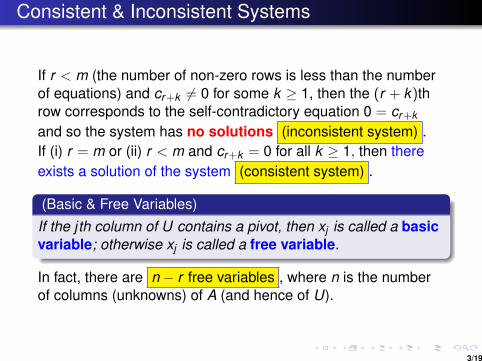
If r < m (the number of non-zero rows is less than the numberof equations) and cr+k 6= 0 for some k ≥ 1, then the (r + k)throw corresponds to the self-contradictory equation 0 = cr+k
and so the system has no solutions (inconsistent system) .If (i) r = m or (ii) r < m and cr+k = 0 for all k ≥ 1, then thereexists a solution of the system (consistent system) .
(Basic & Free Variables)If the jth column of U contains a pivot, then xj is called a basicvariable; otherwise xj is called a free variable.
In fact, there are n − r free variables , where n is the numberof columns (unknowns) of A (and hence of U).
3/19

Consistent & Inconsistent Systems
If r < m (the number of non-zero rows is less than the numberof equations) and cr+k 6= 0 for some k ≥ 1, then the (r + k)throw corresponds to the self-contradictory equation 0 = cr+k
and so the system has no solutions (inconsistent system) .
If (i) r = m or (ii) r < m and cr+k = 0 for all k ≥ 1, then thereexists a solution of the system (consistent system) .
(Basic & Free Variables)If the jth column of U contains a pivot, then xj is called a basicvariable; otherwise xj is called a free variable.
In fact, there are n − r free variables , where n is the numberof columns (unknowns) of A (and hence of U).
3/19

Consistent & Inconsistent Systems
If r < m (the number of non-zero rows is less than the numberof equations) and cr+k 6= 0 for some k ≥ 1, then the (r + k)throw corresponds to the self-contradictory equation 0 = cr+k
and so the system has no solutions (inconsistent system) .If (i) r = m or (ii) r < m and cr+k = 0 for all k ≥ 1, then thereexists a solution of the system (consistent system) .
(Basic & Free Variables)If the jth column of U contains a pivot, then xj is called a basicvariable; otherwise xj is called a free variable.
In fact, there are n − r free variables , where n is the numberof columns (unknowns) of A (and hence of U).
3/19

Consistent & Inconsistent Systems
If r < m (the number of non-zero rows is less than the numberof equations) and cr+k 6= 0 for some k ≥ 1, then the (r + k)throw corresponds to the self-contradictory equation 0 = cr+k
and so the system has no solutions (inconsistent system) .If (i) r = m or (ii) r < m and cr+k = 0 for all k ≥ 1, then thereexists a solution of the system (consistent system) .
(Basic & Free Variables)If the jth column of U contains a pivot, then xj is called a basicvariable;
otherwise xj is called a free variable.
In fact, there are n − r free variables , where n is the numberof columns (unknowns) of A (and hence of U).
3/19

Consistent & Inconsistent Systems
If r < m (the number of non-zero rows is less than the numberof equations) and cr+k 6= 0 for some k ≥ 1, then the (r + k)throw corresponds to the self-contradictory equation 0 = cr+k
and so the system has no solutions (inconsistent system) .If (i) r = m or (ii) r < m and cr+k = 0 for all k ≥ 1, then thereexists a solution of the system (consistent system) .
(Basic & Free Variables)If the jth column of U contains a pivot, then xj is called a basicvariable; otherwise xj is called a free variable.
In fact, there are n − r free variables , where n is the numberof columns (unknowns) of A (and hence of U).
3/19

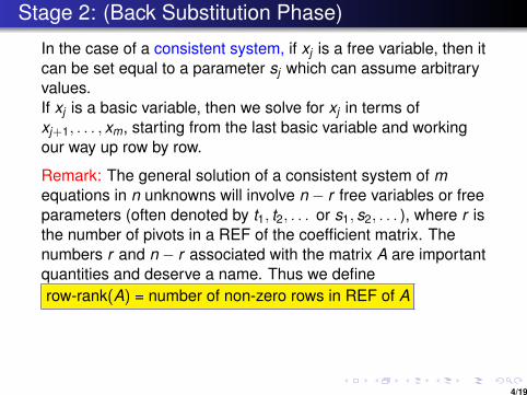
Stage 2: (Back Substitution Phase)
In the case of a consistent system, if xj is a free variable, then itcan be set equal to a parameter sj which can assume arbitraryvalues.
If xj is a basic variable, then we solve for xj in terms ofxj+1, . . . , xm, starting from the last basic variable and workingour way up row by row.
Remark: The general solution of a consistent system of mequations in n unknowns will involve n − r free variables or freeparameters (often denoted by t1, t2, . . . or s1, s2, . . . ), where r isthe number of pivots in a REF of the coefficient matrix. Thenumbers r and n − r associated with the matrix A are importantquantities and deserve a name. Thus we definerow-rank(A) = number of non-zero rows in REF of A
nullity(A) = number of free variables in the solution of AX = 0.
Since the homogeneous system Ax = 0 is always consistent,we see that nullity(A) = n−row-rank(A).
4/19
Stage 2: (Back Substitution Phase)
In the case of a consistent system, if xj is a free variable, then itcan be set equal to a parameter sj which can assume arbitraryvalues.If xj is a basic variable, then we solve for xj in terms ofxj+1, . . . , xm, starting from the last basic variable and workingour way up row by row.
Remark: The general solution of a consistent system of mequations in n unknowns will involve n − r free variables or freeparameters (often denoted by t1, t2, . . . or s1, s2, . . . ), where r isthe number of pivots in a REF of the coefficient matrix. Thenumbers r and n − r associated with the matrix A are importantquantities and deserve a name. Thus we definerow-rank(A) = number of non-zero rows in REF of A
nullity(A) = number of free variables in the solution of AX = 0.
Since the homogeneous system Ax = 0 is always consistent,we see that nullity(A) = n−row-rank(A).
4/19

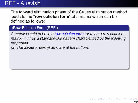
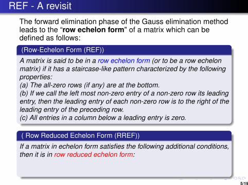
REF - A revisitThe forward elimination phase of the Gauss elimination methodleads to the “row echelon form" of a matrix which can bedefined as follows:
(Row-Echelon Form (REF))
A matrix is said to be in a row echelon form (or to be a row echelonmatrix) if it has a staircase-like pattern characterized by the followingproperties:(a) The all-zero rows (if any) are at the bottom.(b) If we call the left most non-zero entry of a non-zero row its leadingentry, then the leading entry of each non-zero row is to the right of theleading entry of the preceding row.(c) All entries in a column below a leading entry is zero.
( Row Reduced Echelon Form (RREF))
If a matrix in echelon form satisfies the following additional conditions,then it is in row reduced echelon form:(d) The leading entry in each nonzero row is 1.(e) Each leading 1 is the only nonzero entry in its column.
5/19

REF - A revisitThe forward elimination phase of the Gauss elimination methodleads to the “row echelon form" of a matrix which can bedefined as follows:
(Row-Echelon Form (REF))
A matrix is said to be in a row echelon form (or to be a row echelonmatrix) if it has a staircase-like pattern characterized by the followingproperties:
(a) The all-zero rows (if any) are at the bottom.(b) If we call the left most non-zero entry of a non-zero row its leadingentry, then the leading entry of each non-zero row is to the right of theleading entry of the preceding row.(c) All entries in a column below a leading entry is zero.
( Row Reduced Echelon Form (RREF))
If a matrix in echelon form satisfies the following additional conditions,then it is in row reduced echelon form:(d) The leading entry in each nonzero row is 1.(e) Each leading 1 is the only nonzero entry in its column.
5/19
REF - A revisitThe forward elimination phase of the Gauss elimination methodleads to the “row echelon form" of a matrix which can bedefined as follows:
(Row-Echelon Form (REF))
A matrix is said to be in a row echelon form (or to be a row echelonmatrix) if it has a staircase-like pattern characterized by the followingproperties:(a) The all-zero rows (if any) are at the bottom.
(b) If we call the left most non-zero entry of a non-zero row its leadingentry, then the leading entry of each non-zero row is to the right of theleading entry of the preceding row.(c) All entries in a column below a leading entry is zero.
( Row Reduced Echelon Form (RREF))
If a matrix in echelon form satisfies the following additional conditions,then it is in row reduced echelon form:(d) The leading entry in each nonzero row is 1.(e) Each leading 1 is the only nonzero entry in its column.
5/19

REF - A revisitThe forward elimination phase of the Gauss elimination methodleads to the “row echelon form" of a matrix which can bedefined as follows:
(Row-Echelon Form (REF))
A matrix is said to be in a row echelon form (or to be a row echelonmatrix) if it has a staircase-like pattern characterized by the followingproperties:(a) The all-zero rows (if any) are at the bottom.(b) If we call the left most non-zero entry of a non-zero row its leadingentry, then the leading entry of each non-zero row is to the right of theleading entry of the preceding row.
(c) All entries in a column below a leading entry is zero.
( Row Reduced Echelon Form (RREF))
If a matrix in echelon form satisfies the following additional conditions,then it is in row reduced echelon form:(d) The leading entry in each nonzero row is 1.(e) Each leading 1 is the only nonzero entry in its column.
5/19

REF - A revisitThe forward elimination phase of the Gauss elimination methodleads to the “row echelon form" of a matrix which can bedefined as follows:
(Row-Echelon Form (REF))
A matrix is said to be in a row echelon form (or to be a row echelonmatrix) if it has a staircase-like pattern characterized by the followingproperties:(a) The all-zero rows (if any) are at the bottom.(b) If we call the left most non-zero entry of a non-zero row its leadingentry, then the leading entry of each non-zero row is to the right of theleading entry of the preceding row.(c) All entries in a column below a leading entry is zero.
( Row Reduced Echelon Form (RREF))
If a matrix in echelon form satisfies the following additional conditions,then it is in row reduced echelon form:(d) The leading entry in each nonzero row is 1.(e) Each leading 1 is the only nonzero entry in its column.
5/19
REF - A revisitThe forward elimination phase of the Gauss elimination methodleads to the “row echelon form" of a matrix which can bedefined as follows:
(Row-Echelon Form (REF))
A matrix is said to be in a row echelon form (or to be a row echelonmatrix) if it has a staircase-like pattern characterized by the followingproperties:(a) The all-zero rows (if any) are at the bottom.(b) If we call the left most non-zero entry of a non-zero row its leadingentry, then the leading entry of each non-zero row is to the right of theleading entry of the preceding row.(c) All entries in a column below a leading entry is zero.
( Row Reduced Echelon Form (RREF))
If a matrix in echelon form satisfies the following additional conditions,then it is in row reduced echelon form:
(d) The leading entry in each nonzero row is 1.(e) Each leading 1 is the only nonzero entry in its column.
5/19

REF - A revisitThe forward elimination phase of the Gauss elimination methodleads to the “row echelon form" of a matrix which can bedefined as follows:
(Row-Echelon Form (REF))
A matrix is said to be in a row echelon form (or to be a row echelonmatrix) if it has a staircase-like pattern characterized by the followingproperties:(a) The all-zero rows (if any) are at the bottom.(b) If we call the left most non-zero entry of a non-zero row its leadingentry, then the leading entry of each non-zero row is to the right of theleading entry of the preceding row.(c) All entries in a column below a leading entry is zero.
( Row Reduced Echelon Form (RREF))
If a matrix in echelon form satisfies the following additional conditions,then it is in row reduced echelon form:(d) The leading entry in each nonzero row is 1.
(e) Each leading 1 is the only nonzero entry in its column.
5/19

REF - A revisitThe forward elimination phase of the Gauss elimination methodleads to the “row echelon form" of a matrix which can bedefined as follows:
(Row-Echelon Form (REF))
A matrix is said to be in a row echelon form (or to be a row echelonmatrix) if it has a staircase-like pattern characterized by the followingproperties:(a) The all-zero rows (if any) are at the bottom.(b) If we call the left most non-zero entry of a non-zero row its leadingentry, then the leading entry of each non-zero row is to the right of theleading entry of the preceding row.(c) All entries in a column below a leading entry is zero.
( Row Reduced Echelon Form (RREF))
If a matrix in echelon form satisfies the following additional conditions,then it is in row reduced echelon form:(d) The leading entry in each nonzero row is 1.(e) Each leading 1 is the only nonzero entry in its column.
5/19

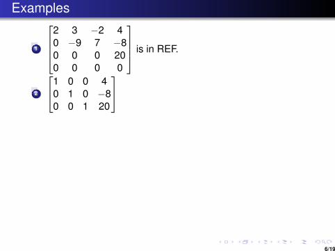
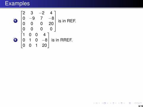
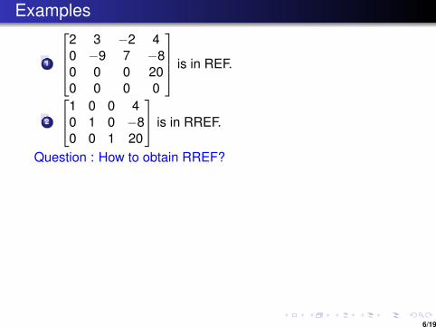
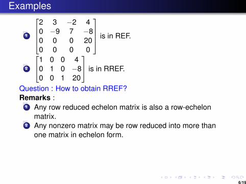
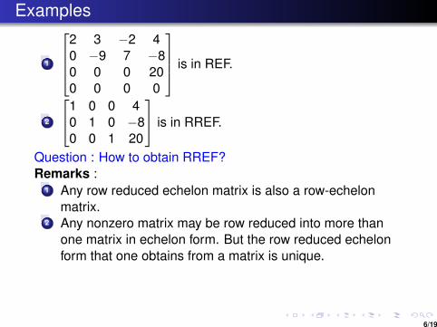
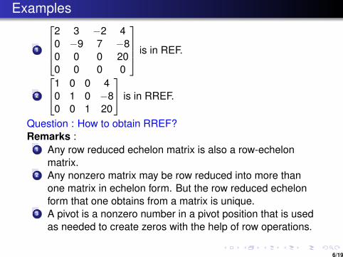
Examples
1
2 3 −2 40 −9 7 −80 0 0 200 0 0 0
is in REF.
2
1 0 0 40 1 0 −80 0 1 20
is in RREF.
Question : How to obtain RREF?Remarks :
1 Any row reduced echelon matrix is also a row-echelonmatrix.
2 Any nonzero matrix may be row reduced into more thanone matrix in echelon form. But the row reduced echelonform that one obtains from a matrix is unique.
3 A pivot is a nonzero number in a pivot position that is usedas needed to create zeros with the help of row operations.
4 Different sequences of row operations might involve adifferent set of pivots.
6/19

Examples
1
2 3 −2 40 −9 7 −80 0 0 200 0 0 0
is in REF.
2
1 0 0 40 1 0 −80 0 1 20
is in RREF.
Question : How to obtain RREF?
Remarks :1 Any row reduced echelon matrix is also a row-echelon
matrix.2 Any nonzero matrix may be row reduced into more than
one matrix in echelon form. But the row reduced echelonform that one obtains from a matrix is unique.
3 A pivot is a nonzero number in a pivot position that is usedas needed to create zeros with the help of row operations.
4 Different sequences of row operations might involve adifferent set of pivots.
6/19

Examples
1
2 3 −2 40 −9 7 −80 0 0 200 0 0 0
is in REF.
2
1 0 0 40 1 0 −80 0 1 20
is in RREF.
Question : How to obtain RREF?Remarks :
1 Any row reduced echelon matrix is also a row-echelonmatrix.
2 Any nonzero matrix may be row reduced into more thanone matrix in echelon form. But the row reduced echelonform that one obtains from a matrix is unique.
3 A pivot is a nonzero number in a pivot position that is usedas needed to create zeros with the help of row operations.
4 Different sequences of row operations might involve adifferent set of pivots.
6/19
Examples
1
2 3 −2 40 −9 7 −80 0 0 200 0 0 0
is in REF.
2
1 0 0 40 1 0 −80 0 1 20
is in RREF.
Question : How to obtain RREF?Remarks :
1 Any row reduced echelon matrix is also a row-echelonmatrix.
2 Any nonzero matrix may be row reduced into more thanone matrix in echelon form.
But the row reduced echelonform that one obtains from a matrix is unique.
3 A pivot is a nonzero number in a pivot position that is usedas needed to create zeros with the help of row operations.
4 Different sequences of row operations might involve adifferent set of pivots.
6/19
Examples
1
2 3 −2 40 −9 7 −80 0 0 200 0 0 0
is in REF.
2
1 0 0 40 1 0 −80 0 1 20
is in RREF.
Question : How to obtain RREF?Remarks :
1 Any row reduced echelon matrix is also a row-echelonmatrix.
2 Any nonzero matrix may be row reduced into more thanone matrix in echelon form. But the row reduced echelonform that one obtains from a matrix is unique.
3 A pivot is a nonzero number in a pivot position that is usedas needed to create zeros with the help of row operations.
4 Different sequences of row operations might involve adifferent set of pivots.
6/19
Examples
1
2 3 −2 40 −9 7 −80 0 0 200 0 0 0
is in REF.
2
1 0 0 40 1 0 −80 0 1 20
is in RREF.
Question : How to obtain RREF?Remarks :
1 Any row reduced echelon matrix is also a row-echelonmatrix.
2 Any nonzero matrix may be row reduced into more thanone matrix in echelon form. But the row reduced echelonform that one obtains from a matrix is unique.
3 A pivot is a nonzero number in a pivot position that is usedas needed to create zeros with the help of row operations.
4 Different sequences of row operations might involve adifferent set of pivots.
6/19

Examples
1
2 3 −2 40 −9 7 −80 0 0 200 0 0 0
is in REF.
2
1 0 0 40 1 0 −80 0 1 20
is in RREF.
Question : How to obtain RREF?Remarks :
1 Any row reduced echelon matrix is also a row-echelonmatrix.
2 Any nonzero matrix may be row reduced into more thanone matrix in echelon form. But the row reduced echelonform that one obtains from a matrix is unique.
3 A pivot is a nonzero number in a pivot position that is usedas needed to create zeros with the help of row operations.
4 Different sequences of row operations might involve adifferent set of pivots. 6/19

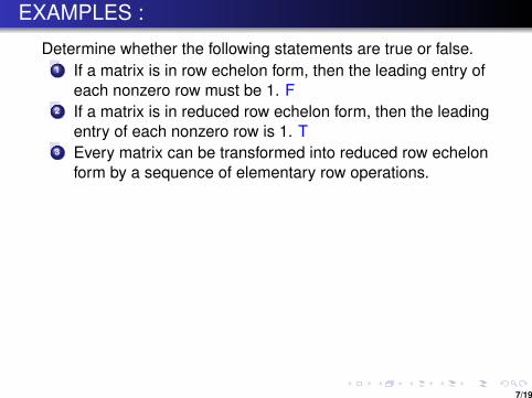
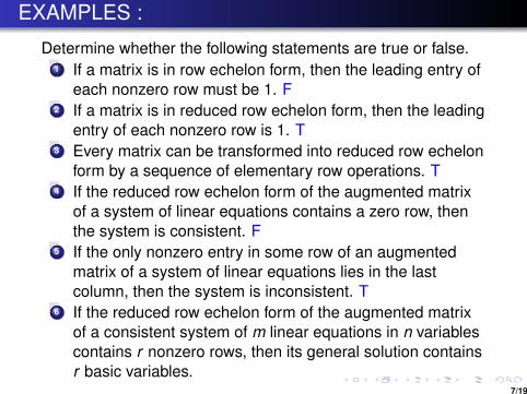
EXAMPLES :
Determine whether the following statements are true or false.1 If a matrix is in row echelon form, then the leading entry of
each nonzero row must be 1.
F2 If a matrix is in reduced row echelon form, then the leading
entry of each nonzero row is 1. T3 Every matrix can be transformed into reduced row echelon
form by a sequence of elementary row operations. T4 If the reduced row echelon form of the augmented matrix
of a system of linear equations contains a zero row, thenthe system is consistent. F
5 If the only nonzero entry in some row of an augmentedmatrix of a system of linear equations lies in the lastcolumn, then the system is inconsistent. T
6 If the reduced row echelon form of the augmented matrixof a consistent system of m linear equations in n variablescontains r nonzero rows, then its general solution containsr basic variables. T (number of free variables = n − r ).
7/19

EXAMPLES :
Determine whether the following statements are true or false.1 If a matrix is in row echelon form, then the leading entry of
each nonzero row must be 1. F2 If a matrix is in reduced row echelon form, then the leading
entry of each nonzero row is 1.
T3 Every matrix can be transformed into reduced row echelon
form by a sequence of elementary row operations. T4 If the reduced row echelon form of the augmented matrix
of a system of linear equations contains a zero row, thenthe system is consistent. F
5 If the only nonzero entry in some row of an augmentedmatrix of a system of linear equations lies in the lastcolumn, then the system is inconsistent. T
6 If the reduced row echelon form of the augmented matrixof a consistent system of m linear equations in n variablescontains r nonzero rows, then its general solution containsr basic variables. T (number of free variables = n − r ).
7/19
EXAMPLES :
Determine whether the following statements are true or false.1 If a matrix is in row echelon form, then the leading entry of
each nonzero row must be 1. F2 If a matrix is in reduced row echelon form, then the leading
entry of each nonzero row is 1. T3 Every matrix can be transformed into reduced row echelon
form by a sequence of elementary row operations.
T4 If the reduced row echelon form of the augmented matrix
of a system of linear equations contains a zero row, thenthe system is consistent. F
5 If the only nonzero entry in some row of an augmentedmatrix of a system of linear equations lies in the lastcolumn, then the system is inconsistent. T
6 If the reduced row echelon form of the augmented matrixof a consistent system of m linear equations in n variablescontains r nonzero rows, then its general solution containsr basic variables. T (number of free variables = n − r ).
7/19

EXAMPLES :
Determine whether the following statements are true or false.1 If a matrix is in row echelon form, then the leading entry of
each nonzero row must be 1. F2 If a matrix is in reduced row echelon form, then the leading
entry of each nonzero row is 1. T3 Every matrix can be transformed into reduced row echelon
form by a sequence of elementary row operations. T4 If the reduced row echelon form of the augmented matrix
of a system of linear equations contains a zero row, thenthe system is consistent.
F5 If the only nonzero entry in some row of an augmented
matrix of a system of linear equations lies in the lastcolumn, then the system is inconsistent. T
6 If the reduced row echelon form of the augmented matrixof a consistent system of m linear equations in n variablescontains r nonzero rows, then its general solution containsr basic variables. T (number of free variables = n − r ).
7/19

EXAMPLES :
Determine whether the following statements are true or false.1 If a matrix is in row echelon form, then the leading entry of
each nonzero row must be 1. F2 If a matrix is in reduced row echelon form, then the leading
entry of each nonzero row is 1. T3 Every matrix can be transformed into reduced row echelon
form by a sequence of elementary row operations. T4 If the reduced row echelon form of the augmented matrix
of a system of linear equations contains a zero row, thenthe system is consistent. F
5 If the only nonzero entry in some row of an augmentedmatrix of a system of linear equations lies in the lastcolumn, then the system is inconsistent.
T6 If the reduced row echelon form of the augmented matrix
of a consistent system of m linear equations in n variablescontains r nonzero rows, then its general solution containsr basic variables. T (number of free variables = n − r ).
7/19
EXAMPLES :
Determine whether the following statements are true or false.1 If a matrix is in row echelon form, then the leading entry of
each nonzero row must be 1. F2 If a matrix is in reduced row echelon form, then the leading
entry of each nonzero row is 1. T3 Every matrix can be transformed into reduced row echelon
form by a sequence of elementary row operations. T4 If the reduced row echelon form of the augmented matrix
of a system of linear equations contains a zero row, thenthe system is consistent. F
5 If the only nonzero entry in some row of an augmentedmatrix of a system of linear equations lies in the lastcolumn, then the system is inconsistent. T
6 If the reduced row echelon form of the augmented matrixof a consistent system of m linear equations in n variablescontains r nonzero rows, then its general solution containsr basic variables.
T (number of free variables = n − r ).
7/19

EXAMPLES :
Determine whether the following statements are true or false.1 If a matrix is in row echelon form, then the leading entry of
each nonzero row must be 1. F2 If a matrix is in reduced row echelon form, then the leading
entry of each nonzero row is 1. T3 Every matrix can be transformed into reduced row echelon
form by a sequence of elementary row operations. T4 If the reduced row echelon form of the augmented matrix
of a system of linear equations contains a zero row, thenthe system is consistent. F
5 If the only nonzero entry in some row of an augmentedmatrix of a system of linear equations lies in the lastcolumn, then the system is inconsistent. T
6 If the reduced row echelon form of the augmented matrixof a consistent system of m linear equations in n variablescontains r nonzero rows, then its general solution containsr basic variables. T
(number of free variables = n − r ).
7/19

EXAMPLES :
Determine whether the following statements are true or false.1 If a matrix is in row echelon form, then the leading entry of
each nonzero row must be 1. F2 If a matrix is in reduced row echelon form, then the leading
entry of each nonzero row is 1. T3 Every matrix can be transformed into reduced row echelon
form by a sequence of elementary row operations. T4 If the reduced row echelon form of the augmented matrix
of a system of linear equations contains a zero row, thenthe system is consistent. F
5 If the only nonzero entry in some row of an augmentedmatrix of a system of linear equations lies in the lastcolumn, then the system is inconsistent. T
6 If the reduced row echelon form of the augmented matrixof a consistent system of m linear equations in n variablescontains r nonzero rows, then its general solution containsr basic variables. T (number of free variables = n − r ).
7/19

More Examples - REF, RREF
Determine whether the following matrices in REF, RREF :
1
1 2 3 4 50 0 1 −1 20 0 0 1 5
is an example of a matrix in REF, not
RREF.
2
1 0 0 0 10 1 0 0 20 0 0 1 3
is in RREF. Is it in REF?? YES.
3 The matrix
2 −1 2 1 50 1 1 −3 30 2 0 0 50 0 0 3 2
is NOT in REF.
4
1 0 0 1/2 0 10 0 1 −1/3 0 20 0 0 0 1 3
is in RREF and hence in REF.
Note that the left side of a matrix in RREF need not be identitymatrix.
8/19

More Examples - REF, RREF
Determine whether the following matrices in REF, RREF :
1
1 2 3 4 50 0 1 −1 20 0 0 1 5
is an example of a matrix in REF,
not
RREF.
2
1 0 0 0 10 1 0 0 20 0 0 1 3
is in RREF. Is it in REF?? YES.
3 The matrix
2 −1 2 1 50 1 1 −3 30 2 0 0 50 0 0 3 2
is NOT in REF.
4
1 0 0 1/2 0 10 0 1 −1/3 0 20 0 0 0 1 3
is in RREF and hence in REF.
Note that the left side of a matrix in RREF need not be identitymatrix.
8/19

More Examples - REF, RREF
Determine whether the following matrices in REF, RREF :
1
1 2 3 4 50 0 1 −1 20 0 0 1 5
is an example of a matrix in REF, not
RREF.
2
1 0 0 0 10 1 0 0 20 0 0 1 3
is in RREF. Is it in REF?? YES.
3 The matrix
2 −1 2 1 50 1 1 −3 30 2 0 0 50 0 0 3 2
is NOT in REF.
4
1 0 0 1/2 0 10 0 1 −1/3 0 20 0 0 0 1 3
is in RREF and hence in REF.
Note that the left side of a matrix in RREF need not be identitymatrix.
8/19

More Examples - REF, RREF
Determine whether the following matrices in REF, RREF :
1
1 2 3 4 50 0 1 −1 20 0 0 1 5
is an example of a matrix in REF, not
RREF.
2
1 0 0 0 10 1 0 0 20 0 0 1 3
is in RREF. Is it in REF?? YES.
3 The matrix
2 −1 2 1 50 1 1 −3 30 2 0 0 50 0 0 3 2
is NOT in REF.
4
1 0 0 1/2 0 10 0 1 −1/3 0 20 0 0 0 1 3
is in RREF and hence in REF.
Note that the left side of a matrix in RREF need not be identitymatrix.
8/19
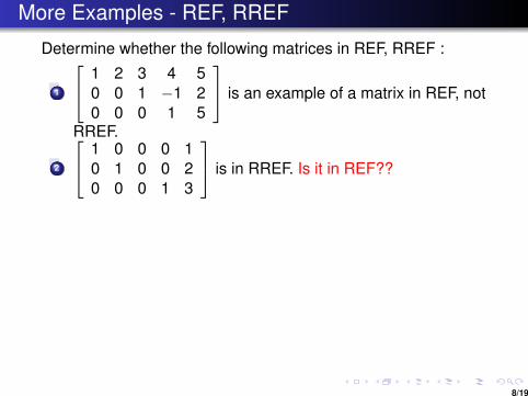
More Examples - REF, RREF
Determine whether the following matrices in REF, RREF :
1
1 2 3 4 50 0 1 −1 20 0 0 1 5
is an example of a matrix in REF, not
RREF.
2
1 0 0 0 10 1 0 0 20 0 0 1 3
is in RREF. Is it in REF??
YES.
3 The matrix
2 −1 2 1 50 1 1 −3 30 2 0 0 50 0 0 3 2
is NOT in REF.
4
1 0 0 1/2 0 10 0 1 −1/3 0 20 0 0 0 1 3
is in RREF and hence in REF.
Note that the left side of a matrix in RREF need not be identitymatrix.
8/19

More Examples - REF, RREF
Determine whether the following matrices in REF, RREF :
1
1 2 3 4 50 0 1 −1 20 0 0 1 5
is an example of a matrix in REF, not
RREF.
2
1 0 0 0 10 1 0 0 20 0 0 1 3
is in RREF. Is it in REF?? YES.
3 The matrix
2 −1 2 1 50 1 1 −3 30 2 0 0 50 0 0 3 2
is NOT in REF.
4
1 0 0 1/2 0 10 0 1 −1/3 0 20 0 0 0 1 3
is in RREF and hence in REF.
Note that the left side of a matrix in RREF need not be identitymatrix.
8/19

More Examples - REF, RREF
Determine whether the following matrices in REF, RREF :
1
1 2 3 4 50 0 1 −1 20 0 0 1 5
is an example of a matrix in REF, not
RREF.
2
1 0 0 0 10 1 0 0 20 0 0 1 3
is in RREF. Is it in REF?? YES.
3 The matrix
2 −1 2 1 50 1 1 −3 30 2 0 0 50 0 0 3 2
is NOT in REF.
4
1 0 0 1/2 0 10 0 1 −1/3 0 20 0 0 0 1 3
is in RREF and hence in REF.
Note that the left side of a matrix in RREF need not be identitymatrix.
8/19
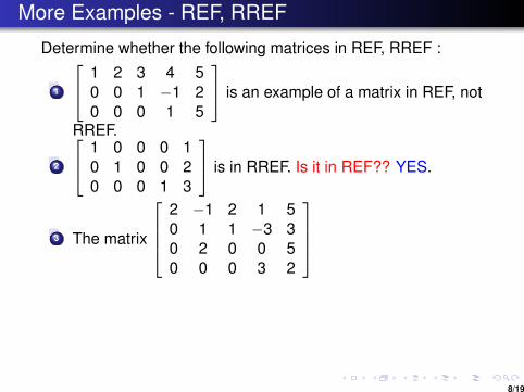
More Examples - REF, RREF
Determine whether the following matrices in REF, RREF :
1
1 2 3 4 50 0 1 −1 20 0 0 1 5
is an example of a matrix in REF, not
RREF.
2
1 0 0 0 10 1 0 0 20 0 0 1 3
is in RREF. Is it in REF?? YES.
3 The matrix
2 −1 2 1 50 1 1 −3 30 2 0 0 50 0 0 3 2
is NOT in REF.
4
1 0 0 1/2 0 10 0 1 −1/3 0 20 0 0 0 1 3
is in RREF and hence in REF.
Note that the left side of a matrix in RREF need not be identitymatrix.
8/19
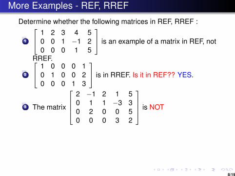
More Examples - REF, RREF
Determine whether the following matrices in REF, RREF :
1
1 2 3 4 50 0 1 −1 20 0 0 1 5
is an example of a matrix in REF, not
RREF.
2
1 0 0 0 10 1 0 0 20 0 0 1 3
is in RREF. Is it in REF?? YES.
3 The matrix
2 −1 2 1 50 1 1 −3 30 2 0 0 50 0 0 3 2
is NOT
in REF.
4
1 0 0 1/2 0 10 0 1 −1/3 0 20 0 0 0 1 3
is in RREF and hence in REF.
Note that the left side of a matrix in RREF need not be identitymatrix.
8/19

More Examples - REF, RREF
Determine whether the following matrices in REF, RREF :
1
1 2 3 4 50 0 1 −1 20 0 0 1 5
is an example of a matrix in REF, not
RREF.
2
1 0 0 0 10 1 0 0 20 0 0 1 3
is in RREF. Is it in REF?? YES.
3 The matrix
2 −1 2 1 50 1 1 −3 30 2 0 0 50 0 0 3 2
is NOT in REF.
4
1 0 0 1/2 0 10 0 1 −1/3 0 20 0 0 0 1 3
is in RREF and hence in REF.
Note that the left side of a matrix in RREF need not be identitymatrix.
8/19

More Examples - REF, RREF
Determine whether the following matrices in REF, RREF :
1
1 2 3 4 50 0 1 −1 20 0 0 1 5
is an example of a matrix in REF, not
RREF.
2
1 0 0 0 10 1 0 0 20 0 0 1 3
is in RREF. Is it in REF?? YES.
3 The matrix
2 −1 2 1 50 1 1 −3 30 2 0 0 50 0 0 3 2
is NOT in REF.
4
1 0 0 1/2 0 10 0 1 −1/3 0 20 0 0 0 1 3
is in RREF
and hence in REF.
Note that the left side of a matrix in RREF need not be identitymatrix.
8/19

More Examples - REF, RREF
Determine whether the following matrices in REF, RREF :
1
1 2 3 4 50 0 1 −1 20 0 0 1 5
is an example of a matrix in REF, not
RREF.
2
1 0 0 0 10 1 0 0 20 0 0 1 3
is in RREF. Is it in REF?? YES.
3 The matrix
2 −1 2 1 50 1 1 −3 30 2 0 0 50 0 0 3 2
is NOT in REF.
4
1 0 0 1/2 0 10 0 1 −1/3 0 20 0 0 0 1 3
is in RREF and hence in REF.
Note that the left side of a matrix in RREF need not be identitymatrix.
8/19

More Examples - REF, RREF
Determine whether the following matrices in REF, RREF :
1
1 2 3 4 50 0 1 −1 20 0 0 1 5
is an example of a matrix in REF, not
RREF.
2
1 0 0 0 10 1 0 0 20 0 0 1 3
is in RREF. Is it in REF?? YES.
3 The matrix
2 −1 2 1 50 1 1 −3 30 2 0 0 50 0 0 3 2
is NOT in REF.
4
1 0 0 1/2 0 10 0 1 −1/3 0 20 0 0 0 1 3
is in RREF and hence in REF.
Note that the left side of a matrix in RREF need not be identitymatrix.
8/19

Solution given REF
Example
Consider the REF form of the augmented matrix given by1 1 2 3 20 1 5 0 10 0 0 1 20 0 0 0 0
.
In this case r = 3 (number of pivots) and n = 4 (number ofvariables).Note that x3 is a free variable and x1, x2, x4 are basicvariables.Back substitution yields x4 = 2,
x2 + 5x3 = 1 =⇒ x2 = 1− 5x3 = 1− 5sx1 + x2 + 2x3 + 3x4 = 2 =⇒ x1 = 2− (1− 5s)− 2s − 3× 2
=⇒ x1 = −5 + 3s.
We get infinitely many solutions (since x3 is a free parameter).
9/19

Solution given REF
ExampleConsider the REF form of the augmented matrix given by
1 1 2 3 20 1 5 0 10 0 0 1 20 0 0 0 0
.
In this case r = 3 (number of pivots) and n = 4 (number ofvariables).Note that x3 is a free variable and x1, x2, x4 are basicvariables.Back substitution yields x4 = 2,
x2 + 5x3 = 1 =⇒ x2 = 1− 5x3 = 1− 5sx1 + x2 + 2x3 + 3x4 = 2 =⇒ x1 = 2− (1− 5s)− 2s − 3× 2
=⇒ x1 = −5 + 3s.
We get infinitely many solutions (since x3 is a free parameter).
9/19

Solution given REF
ExampleConsider the REF form of the augmented matrix given by
1 1 2 3 2
0 1 5 0 10 0 0 1 20 0 0 0 0
.
In this case r = 3 (number of pivots) and n = 4 (number ofvariables).Note that x3 is a free variable and x1, x2, x4 are basicvariables.Back substitution yields x4 = 2,
x2 + 5x3 = 1 =⇒ x2 = 1− 5x3 = 1− 5sx1 + x2 + 2x3 + 3x4 = 2 =⇒ x1 = 2− (1− 5s)− 2s − 3× 2
=⇒ x1 = −5 + 3s.
We get infinitely many solutions (since x3 is a free parameter).
9/19

Solution given REF
ExampleConsider the REF form of the augmented matrix given by
1 1 2 3 20 1 5 0 1
0 0 0 1 20 0 0 0 0
.
In this case r = 3 (number of pivots) and n = 4 (number ofvariables).Note that x3 is a free variable and x1, x2, x4 are basicvariables.Back substitution yields x4 = 2,
x2 + 5x3 = 1 =⇒ x2 = 1− 5x3 = 1− 5sx1 + x2 + 2x3 + 3x4 = 2 =⇒ x1 = 2− (1− 5s)− 2s − 3× 2
=⇒ x1 = −5 + 3s.
We get infinitely many solutions (since x3 is a free parameter).
9/19

Solution given REF
ExampleConsider the REF form of the augmented matrix given by
1 1 2 3 20 1 5 0 10 0 0 1 2
0 0 0 0 0
.
In this case r = 3 (number of pivots) and n = 4 (number ofvariables).Note that x3 is a free variable and x1, x2, x4 are basicvariables.Back substitution yields x4 = 2,
x2 + 5x3 = 1 =⇒ x2 = 1− 5x3 = 1− 5sx1 + x2 + 2x3 + 3x4 = 2 =⇒ x1 = 2− (1− 5s)− 2s − 3× 2
=⇒ x1 = −5 + 3s.
We get infinitely many solutions (since x3 is a free parameter).
9/19
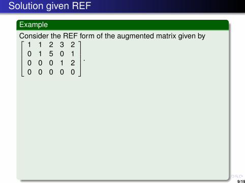
Solution given REF
ExampleConsider the REF form of the augmented matrix given by
1 1 2 3 20 1 5 0 10 0 0 1 20 0 0 0 0
.
In this case r = 3 (number of pivots) and n = 4 (number ofvariables).Note that x3 is a free variable and x1, x2, x4 are basicvariables.Back substitution yields x4 = 2,
x2 + 5x3 = 1 =⇒ x2 = 1− 5x3 = 1− 5sx1 + x2 + 2x3 + 3x4 = 2 =⇒ x1 = 2− (1− 5s)− 2s − 3× 2
=⇒ x1 = −5 + 3s.
We get infinitely many solutions (since x3 is a free parameter).
9/19
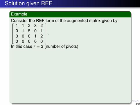
Solution given REF
ExampleConsider the REF form of the augmented matrix given by
1 1 2 3 20 1 5 0 10 0 0 1 20 0 0 0 0
.
In this case r = 3 (number of pivots)
and n = 4 (number ofvariables).Note that x3 is a free variable and x1, x2, x4 are basicvariables.Back substitution yields x4 = 2,
x2 + 5x3 = 1 =⇒ x2 = 1− 5x3 = 1− 5sx1 + x2 + 2x3 + 3x4 = 2 =⇒ x1 = 2− (1− 5s)− 2s − 3× 2
=⇒ x1 = −5 + 3s.
We get infinitely many solutions (since x3 is a free parameter).
9/19
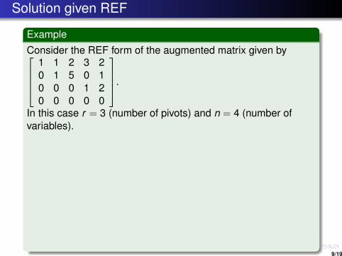
Solution given REF
ExampleConsider the REF form of the augmented matrix given by
1 1 2 3 20 1 5 0 10 0 0 1 20 0 0 0 0
.
In this case r = 3 (number of pivots) and n = 4 (number ofvariables).
Note that x3 is a free variable and x1, x2, x4 are basicvariables.Back substitution yields x4 = 2,
x2 + 5x3 = 1 =⇒ x2 = 1− 5x3 = 1− 5sx1 + x2 + 2x3 + 3x4 = 2 =⇒ x1 = 2− (1− 5s)− 2s − 3× 2
=⇒ x1 = −5 + 3s.
We get infinitely many solutions (since x3 is a free parameter).
9/19

Solution given REF
ExampleConsider the REF form of the augmented matrix given by
1 1 2 3 20 1 5 0 10 0 0 1 20 0 0 0 0
.
In this case r = 3 (number of pivots) and n = 4 (number ofvariables).Note that x3 is a free variable
and x1, x2, x4 are basicvariables.Back substitution yields x4 = 2,
x2 + 5x3 = 1 =⇒ x2 = 1− 5x3 = 1− 5sx1 + x2 + 2x3 + 3x4 = 2 =⇒ x1 = 2− (1− 5s)− 2s − 3× 2
=⇒ x1 = −5 + 3s.
We get infinitely many solutions (since x3 is a free parameter).
9/19

Solution given REF
ExampleConsider the REF form of the augmented matrix given by
1 1 2 3 20 1 5 0 10 0 0 1 20 0 0 0 0
.
In this case r = 3 (number of pivots) and n = 4 (number ofvariables).Note that x3 is a free variable and x1, x2, x4 are basicvariables.
Back substitution yields x4 = 2,
x2 + 5x3 = 1 =⇒ x2 = 1− 5x3 = 1− 5sx1 + x2 + 2x3 + 3x4 = 2 =⇒ x1 = 2− (1− 5s)− 2s − 3× 2
=⇒ x1 = −5 + 3s.
We get infinitely many solutions (since x3 is a free parameter).
9/19

Solution given REF
ExampleConsider the REF form of the augmented matrix given by
1 1 2 3 20 1 5 0 10 0 0 1 20 0 0 0 0
.
In this case r = 3 (number of pivots) and n = 4 (number ofvariables).Note that x3 is a free variable and x1, x2, x4 are basicvariables.Back substitution yields
x4 = 2,
x2 + 5x3 = 1 =⇒ x2 = 1− 5x3 = 1− 5sx1 + x2 + 2x3 + 3x4 = 2 =⇒ x1 = 2− (1− 5s)− 2s − 3× 2
=⇒ x1 = −5 + 3s.
We get infinitely many solutions (since x3 is a free parameter).
9/19

Solution given REF
ExampleConsider the REF form of the augmented matrix given by
1 1 2 3 20 1 5 0 10 0 0 1 20 0 0 0 0
.
In this case r = 3 (number of pivots) and n = 4 (number ofvariables).Note that x3 is a free variable and x1, x2, x4 are basicvariables.Back substitution yields x4 = 2,
x2 + 5x3 = 1 =⇒ x2 = 1− 5x3 = 1− 5sx1 + x2 + 2x3 + 3x4 = 2 =⇒ x1 = 2− (1− 5s)− 2s − 3× 2
=⇒ x1 = −5 + 3s.
We get infinitely many solutions (since x3 is a free parameter).
9/19

Solution given REF
ExampleConsider the REF form of the augmented matrix given by
1 1 2 3 20 1 5 0 10 0 0 1 20 0 0 0 0
.
In this case r = 3 (number of pivots) and n = 4 (number ofvariables).Note that x3 is a free variable and x1, x2, x4 are basicvariables.Back substitution yields x4 = 2,
x2 + 5x3 = 1
=⇒ x2 = 1− 5x3 = 1− 5sx1 + x2 + 2x3 + 3x4 = 2 =⇒ x1 = 2− (1− 5s)− 2s − 3× 2
=⇒ x1 = −5 + 3s.
We get infinitely many solutions (since x3 is a free parameter).
9/19
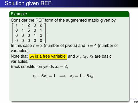
Solution given REF
ExampleConsider the REF form of the augmented matrix given by
1 1 2 3 20 1 5 0 10 0 0 1 20 0 0 0 0
.
In this case r = 3 (number of pivots) and n = 4 (number ofvariables).Note that x3 is a free variable and x1, x2, x4 are basicvariables.Back substitution yields x4 = 2,
x2 + 5x3 = 1 =⇒ x2 = 1− 5x3
= 1− 5sx1 + x2 + 2x3 + 3x4 = 2 =⇒ x1 = 2− (1− 5s)− 2s − 3× 2
=⇒ x1 = −5 + 3s.
We get infinitely many solutions (since x3 is a free parameter).
9/19

Solution given REF
ExampleConsider the REF form of the augmented matrix given by
1 1 2 3 20 1 5 0 10 0 0 1 20 0 0 0 0
.
In this case r = 3 (number of pivots) and n = 4 (number ofvariables).Note that x3 is a free variable and x1, x2, x4 are basicvariables.Back substitution yields x4 = 2,
x2 + 5x3 = 1 =⇒ x2 = 1− 5x3 = 1− 5s
x1 + x2 + 2x3 + 3x4 = 2 =⇒ x1 = 2− (1− 5s)− 2s − 3× 2=⇒ x1 = −5 + 3s.
We get infinitely many solutions (since x3 is a free parameter).
9/19

Solution given REF
ExampleConsider the REF form of the augmented matrix given by
1 1 2 3 20 1 5 0 10 0 0 1 20 0 0 0 0
.
In this case r = 3 (number of pivots) and n = 4 (number ofvariables).Note that x3 is a free variable and x1, x2, x4 are basicvariables.Back substitution yields x4 = 2,
x2 + 5x3 = 1 =⇒ x2 = 1− 5x3 = 1− 5sx1 + x2 + 2x3 + 3x4 = 2
=⇒ x1 = 2− (1− 5s)− 2s − 3× 2=⇒ x1 = −5 + 3s.
We get infinitely many solutions (since x3 is a free parameter).
9/19

Solution given REF
ExampleConsider the REF form of the augmented matrix given by
1 1 2 3 20 1 5 0 10 0 0 1 20 0 0 0 0
.
In this case r = 3 (number of pivots) and n = 4 (number ofvariables).Note that x3 is a free variable and x1, x2, x4 are basicvariables.Back substitution yields x4 = 2,
x2 + 5x3 = 1 =⇒ x2 = 1− 5x3 = 1− 5sx1 + x2 + 2x3 + 3x4 = 2 =⇒ x1 = 2− (1− 5s)− 2s − 3× 2
=⇒ x1 = −5 + 3s.
We get infinitely many solutions (since x3 is a free parameter).
9/19

Solution given REF
ExampleConsider the REF form of the augmented matrix given by
1 1 2 3 20 1 5 0 10 0 0 1 20 0 0 0 0
.
In this case r = 3 (number of pivots) and n = 4 (number ofvariables).Note that x3 is a free variable and x1, x2, x4 are basicvariables.Back substitution yields x4 = 2,
x2 + 5x3 = 1 =⇒ x2 = 1− 5x3 = 1− 5sx1 + x2 + 2x3 + 3x4 = 2 =⇒ x1 = 2− (1− 5s)− 2s − 3× 2
=⇒ x1 = −5 + 3s.
We get infinitely many solutions
(since x3 is a free parameter).
9/19

Solution given REF
ExampleConsider the REF form of the augmented matrix given by
1 1 2 3 20 1 5 0 10 0 0 1 20 0 0 0 0
.
In this case r = 3 (number of pivots) and n = 4 (number ofvariables).Note that x3 is a free variable and x1, x2, x4 are basicvariables.Back substitution yields x4 = 2,
x2 + 5x3 = 1 =⇒ x2 = 1− 5x3 = 1− 5sx1 + x2 + 2x3 + 3x4 = 2 =⇒ x1 = 2− (1− 5s)− 2s − 3× 2
=⇒ x1 = −5 + 3s.
We get infinitely many solutions (since x3 is a free parameter).9/19

Elementary Matrices: Another Viewpoint
An m ×m elementary matrix is a matrix obtained from them ×m identity matrix Im by one of the elementary operations,namely,
1 interchange of two rows,2 multiplying a row by a non-zero scalar,3 adding a scalar multiple of a row to another
row.
That is, an elementary matrix is a matrix which differs from theidentity matrix by one single elementary row operation.
10/19

Elementary Matrices: Another Viewpoint
An m ×m elementary matrix is a matrix obtained from them ×m identity matrix Im by one of the elementary operations,namely,
1 interchange of two rows,
2 multiplying a row by a non-zero scalar,3 adding a scalar multiple of a row to another
row.
That is, an elementary matrix is a matrix which differs from theidentity matrix by one single elementary row operation.
10/19

Elementary Matrices: Another Viewpoint
An m ×m elementary matrix is a matrix obtained from them ×m identity matrix Im by one of the elementary operations,namely,
1 interchange of two rows,2 multiplying a row by a non-zero scalar,
3 adding a scalar multiple of a row to anotherrow.
That is, an elementary matrix is a matrix which differs from theidentity matrix by one single elementary row operation.
10/19

Elementary Matrices: Another Viewpoint
An m ×m elementary matrix is a matrix obtained from them ×m identity matrix Im by one of the elementary operations,namely,
1 interchange of two rows,2 multiplying a row by a non-zero scalar,3 adding a scalar multiple of a row to another
row.
That is, an elementary matrix is a matrix which differs from theidentity matrix by one single elementary row operation.
10/19

Elementary Matrices: Another Viewpoint
An m ×m elementary matrix is a matrix obtained from them ×m identity matrix Im by one of the elementary operations,namely,
1 interchange of two rows,2 multiplying a row by a non-zero scalar,3 adding a scalar multiple of a row to another
row.
That is, an elementary matrix is a matrix which differs from theidentity matrix by one single elementary row operation.
10/19

1. Row Switching Operation
Interchange of two rows - Ri ↔ Rj .
The elementary matrix Ei,j corresponding to this operation on Imof interchanging i th and j th rows.
Ei,j =
C1 . . . Ci . . . Cj . . . Cm
R1 1...
. . .Ri 0 . . . 1...
. . .Rj 1 . . . 0...
. . .Rm 1
Example : Consider I3. R1 ↔ R2 gives E1,2 =
0 1 01 0 00 0 1
..
11/19
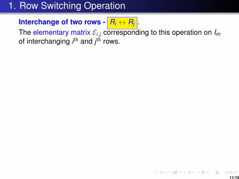
1. Row Switching Operation
Interchange of two rows - Ri ↔ Rj .The elementary matrix Ei,j corresponding to this operation on Imof interchanging i th and j th rows.
Ei,j =
C1 . . . Ci . . . Cj . . . Cm
R1 1...
. . .Ri 0 . . . 1...
. . .Rj 1 . . . 0...
. . .Rm 1
Example : Consider I3.
R1 ↔ R2 gives E1,2 =
0 1 01 0 00 0 1
..
11/19
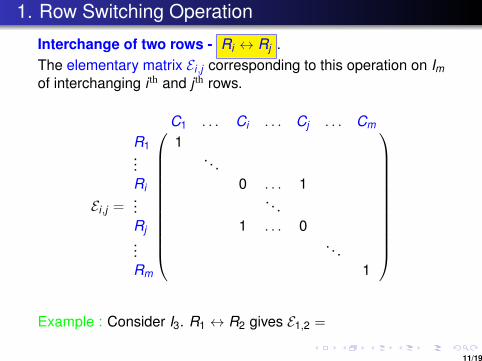
1. Row Switching Operation
Interchange of two rows - Ri ↔ Rj .The elementary matrix Ei,j corresponding to this operation on Imof interchanging i th and j th rows.
Ei,j =
C1 . . . Ci . . . Cj . . . Cm
R1 1...
. . .Ri 0 . . . 1...
. . .Rj 1 . . . 0...
. . .Rm 1
Example : Consider I3. R1 ↔ R2 gives E1,2 =
0 1 01 0 00 0 1
..
11/19

1. Row Switching Operation
Interchange of two rows - Ri ↔ Rj .The elementary matrix Ei,j corresponding to this operation on Imof interchanging i th and j th rows.
Ei,j =
C1 . . . Ci . . . Cj . . . Cm
R1 1...
. . .Ri 0 . . . 1...
. . .Rj 1 . . . 0...
. . .Rm 1
Example : Consider I3. R1 ↔ R2 gives E1,2 =
0 1 01 0 00 0 1
..
11/19

2. Row Multiplying Transformation
Multiplying a row by a non-zero constant - Ri −→ kRi .
Theelementary matrix Ei(k) corresponding to this operation on Im isobtained by multiplying row i of the identity matrix by anon-zero constant k .
Ei(k) =
C1 C2 . . . Ci . . . Cm
R1 1R2 1...
. . .Ri k...
. . .Rm 1
Example : Consider I3. R3 → 7R3 gives E3(7) =
1 0 00 1 00 0 7
.
12/19
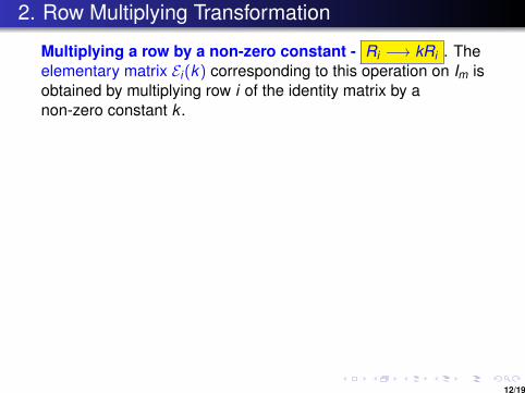
2. Row Multiplying Transformation
Multiplying a row by a non-zero constant - Ri −→ kRi . Theelementary matrix Ei(k) corresponding to this operation on Im isobtained by multiplying row i of the identity matrix by anon-zero constant k .
Ei(k) =
C1 C2 . . . Ci . . . Cm
R1 1R2 1...
. . .Ri k...
. . .Rm 1
Example : Consider I3.
R3 → 7R3 gives E3(7) =
1 0 00 1 00 0 7
.
12/19
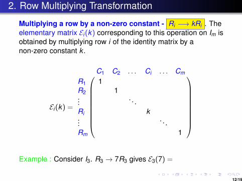
2. Row Multiplying Transformation
Multiplying a row by a non-zero constant - Ri −→ kRi . Theelementary matrix Ei(k) corresponding to this operation on Im isobtained by multiplying row i of the identity matrix by anon-zero constant k .
Ei(k) =
C1 C2 . . . Ci . . . Cm
R1 1R2 1...
. . .Ri k...
. . .Rm 1
Example : Consider I3. R3 → 7R3 gives E3(7) =
1 0 00 1 00 0 7
.
12/19

2. Row Multiplying Transformation
Multiplying a row by a non-zero constant - Ri −→ kRi . Theelementary matrix Ei(k) corresponding to this operation on Im isobtained by multiplying row i of the identity matrix by anon-zero constant k .
Ei(k) =
C1 C2 . . . Ci . . . Cm
R1 1R2 1...
. . .Ri k...
. . .Rm 1
Example : Consider I3. R3 → 7R3 gives E3(7) =
1 0 00 1 00 0 7
.
12/19

3. Row Addition Transformation
Ri −→ Ri + kRj :
The elementary matrix Ei,j(k) correspondingto this operation on Im is obtained by multiplying row j of theidentity matrix by a non-zero constant k and adding with row i .
Ei,j(k) =
C1 . . . Ci . . . Cj . . . Cm
R1 1...
. . .Ri 1 k...
. . .Rj 1...
. . .Rm 1
Example : R2 → R2 + (−3)R1 for I3 gives E2,1(−3) =
1 0 0−3 1 00 0 1
.
13/19
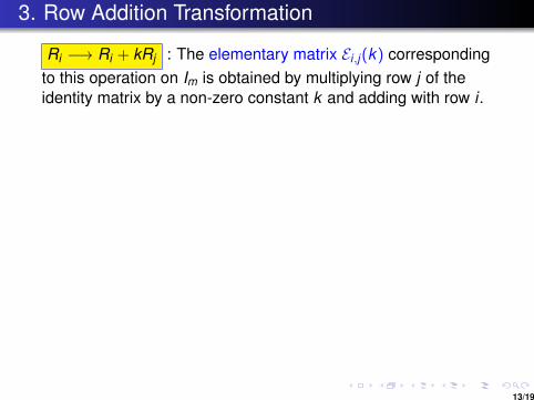
3. Row Addition Transformation
Ri −→ Ri + kRj : The elementary matrix Ei,j(k) correspondingto this operation on Im is obtained by multiplying row j of theidentity matrix by a non-zero constant k and adding with row i .
Ei,j(k) =
C1 . . . Ci . . . Cj . . . Cm
R1 1...
. . .Ri 1 k...
. . .Rj 1...
. . .Rm 1
Example :
R2 → R2 + (−3)R1 for I3 gives E2,1(−3) =
1 0 0−3 1 00 0 1
.
13/19

3. Row Addition Transformation
Ri −→ Ri + kRj : The elementary matrix Ei,j(k) correspondingto this operation on Im is obtained by multiplying row j of theidentity matrix by a non-zero constant k and adding with row i .
Ei,j(k) =
C1 . . . Ci . . . Cj . . . Cm
R1 1...
. . .Ri 1 k...
. . .Rj 1...
. . .Rm 1
Example : R2 → R2 + (−3)R1 for I3 gives E2,1(−3) =
1 0 0−3 1 00 0 1
.
13/19

3. Row Addition Transformation
Ri −→ Ri + kRj : The elementary matrix Ei,j(k) correspondingto this operation on Im is obtained by multiplying row j of theidentity matrix by a non-zero constant k and adding with row i .
Ei,j(k) =
C1 . . . Ci . . . Cj . . . Cm
R1 1...
. . .Ri 1 k...
. . .Rj 1...
. . .Rm 1
Example : R2 → R2 + (−3)R1 for I3 gives E2,1(−3) =
1 0 0−3 1 00 0 1
.
13/19
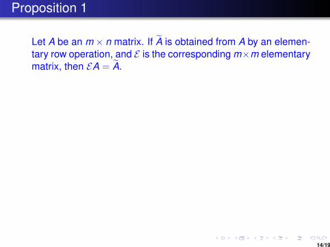
Proposition 1
Let A be an m × n matrix. If A is obtained from A by an elemen-tary row operation, and E is the corresponding m×m elementarymatrix, then EA = A.
Proof :
Let Im =
1 0 · · · 00 1 · · · 0...
.... . .
...0 0 · · · 1
=
eT
1eT
2...
eTm
where ei =
0...1...0
, with 1 is in the i th position, 1 ≤ i ≤ m.
Also, eTi A = A(i), the i th row of A.
14/19
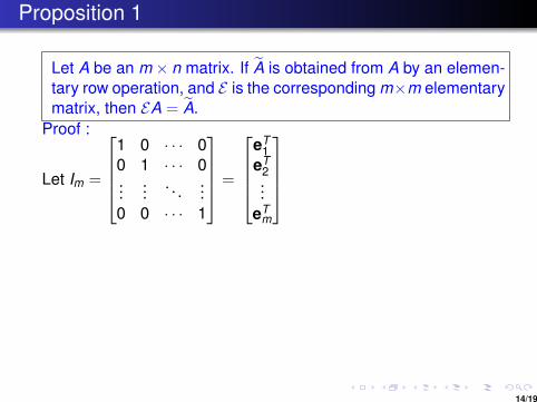

Proposition 1
Let A be an m × n matrix. If A is obtained from A by an elemen-tary row operation, and E is the corresponding m×m elementarymatrix, then EA = A.
Proof :
Let Im =
1 0 · · · 00 1 · · · 0...
.... . .
...0 0 · · · 1
=
eT
1eT
2...
eTm
where ei =
0...1...0
, with 1 is in the i th position, 1 ≤ i ≤ m.
Also, eTi A =
A(i), the i th row of A.
14/19
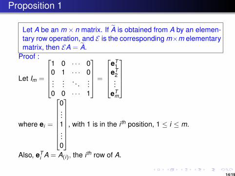
Proposition 1
Let A be an m × n matrix. If A is obtained from A by an elemen-tary row operation, and E is the corresponding m×m elementarymatrix, then EA = A.
Proof :
Let Im =
1 0 · · · 00 1 · · · 0...
.... . .
...0 0 · · · 1
=
eT
1eT
2...
eTm
where ei =
0...1...0
, with 1 is in the i th position, 1 ≤ i ≤ m.
Also, eTi A = A(i), the i th row of A.
14/19

Proposition 1
Let A be an m × n matrix. If A is obtained from A by an elemen-tary row operation, and E is the corresponding m×m elementarymatrix, then EA = A.
Proof :
Let Im =
1 0 · · · 00 1 · · · 0...
.... . .
...0 0 · · · 1
=
eT
1eT
2...
eTm
where ei =
0...1...0
, with 1 is in the i th position, 1 ≤ i ≤ m.
Also, eTi A = A(i), the i th row of A.
14/19

Ri ↔ Rj(i < j)
Ei,jA =
...eT
j...
eTi...
A =
...eT
j A...
eTi A...
=
...A(j)
...A(i)
...
= A.
Ri −→ kRi Ei(k)A =
...
keTi
...
A =
...
keTi A...
=
...
kA(i)...
= A.
Ri −→ Ri + kRj
Ei,j(k)A =
...
eTi + keT
j...
A =
...
(eTi + keT
j )A...
=
...
A(i) + kA(j)...
= A.
15/19

Ri ↔ Rj(i < j) Ei,jA =
...eT
j...
eTi...
A =
...eT
j A...
eTi A...
=
...A(j)
...A(i)
...
= A.
Ri −→ kRi Ei(k)A =
...
keTi
...
A =
...
keTi A...
=
...
kA(i)...
= A.
Ri −→ Ri + kRj
Ei,j(k)A =
...
eTi + keT
j...
A =
...
(eTi + keT
j )A...
=
...
A(i) + kA(j)...
= A.
15/19
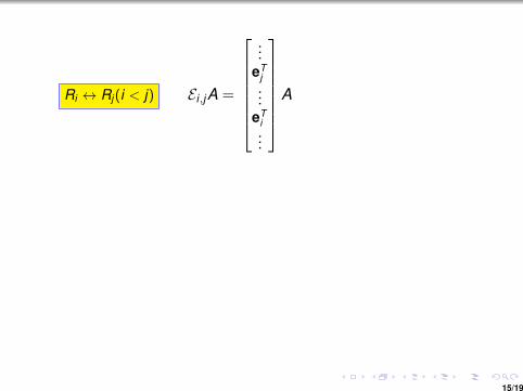
Ri ↔ Rj(i < j) Ei,jA =
...eT
j...
eTi...
A
=
...eT
j A...
eTi A...
=
...A(j)
...A(i)
...
= A.
Ri −→ kRi Ei(k)A =
...
keTi
...
A =
...
keTi A...
=
...
kA(i)...
= A.
Ri −→ Ri + kRj
Ei,j(k)A =
...
eTi + keT
j...
A =
...
(eTi + keT
j )A...
=
...
A(i) + kA(j)...
= A.
15/19

Ri ↔ Rj(i < j) Ei,jA =
...eT
j...
eTi...
A =
...eT
j A...
eTi A...
=
...A(j)
...A(i)
...
= A.
Ri −→ kRi Ei(k)A =
...
keTi
...
A =
...
keTi A...
=
...
kA(i)...
= A.
Ri −→ Ri + kRj
Ei,j(k)A =
...
eTi + keT
j...
A =
...
(eTi + keT
j )A...
=
...
A(i) + kA(j)...
= A.
15/19

Ri ↔ Rj(i < j) Ei,jA =
...eT
j...
eTi...
A =
...eT
j A...
eTi A...
=
...A(j)
...A(i)
...
= A.
Ri −→ kRi Ei(k)A =
...
keTi
...
A =
...
keTi A...
=
...
kA(i)...
= A.
Ri −→ Ri + kRj
Ei,j(k)A =
...
eTi + keT
j...
A =
...
(eTi + keT
j )A...
=
...
A(i) + kA(j)...
= A.
15/19

Ri ↔ Rj(i < j) Ei,jA =
...eT
j...
eTi...
A =
...eT
j A...
eTi A...
=
...A(j)
...A(i)
...
= A.
Ri −→ kRi
Ei(k)A =
...
keTi
...
A =
...
keTi A...
=
...
kA(i)...
= A.
Ri −→ Ri + kRj
Ei,j(k)A =
...
eTi + keT
j...
A =
...
(eTi + keT
j )A...
=
...
A(i) + kA(j)...
= A.
15/19
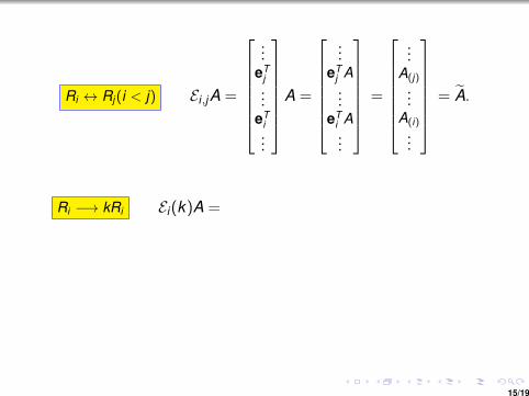
Ri ↔ Rj(i < j) Ei,jA =
...eT
j...
eTi...
A =
...eT
j A...
eTi A...
=
...A(j)
...A(i)
...
= A.
Ri −→ kRi Ei(k)A =
...
keTi
...
A =
...
keTi A...
=
...
kA(i)...
= A.
Ri −→ Ri + kRj
Ei,j(k)A =
...
eTi + keT
j...
A =
...
(eTi + keT
j )A...
=
...
A(i) + kA(j)...
= A.
15/19

Ri ↔ Rj(i < j) Ei,jA =
...eT
j...
eTi...
A =
...eT
j A...
eTi A...
=
...A(j)
...A(i)
...
= A.
Ri −→ kRi Ei(k)A =
...
keTi
...
A
=
...
keTi A...
=
...
kA(i)...
= A.
Ri −→ Ri + kRj
Ei,j(k)A =
...
eTi + keT
j...
A =
...
(eTi + keT
j )A...
=
...
A(i) + kA(j)...
= A.
15/19

Ri ↔ Rj(i < j) Ei,jA =
...eT
j...
eTi...
A =
...eT
j A...
eTi A...
=
...A(j)
...A(i)
...
= A.
Ri −→ kRi Ei(k)A =
...
keTi
...
A =
...
keTi A...
=
...
kA(i)...
= A.
Ri −→ Ri + kRj
Ei,j(k)A =
...
eTi + keT
j...
A =
...
(eTi + keT
j )A...
=
...
A(i) + kA(j)...
= A.
15/19
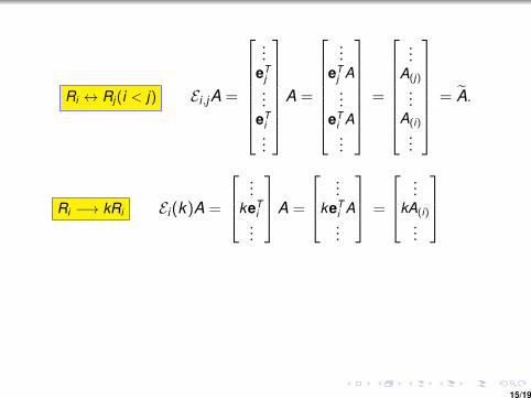
Ri ↔ Rj(i < j) Ei,jA =
...eT
j...
eTi...
A =
...eT
j A...
eTi A...
=
...A(j)
...A(i)
...
= A.
Ri −→ kRi Ei(k)A =
...
keTi
...
A =
...
keTi A...
=
...
kA(i)...
= A.
Ri −→ Ri + kRj
Ei,j(k)A =
...
eTi + keT
j...
A =
...
(eTi + keT
j )A...
=
...
A(i) + kA(j)...
= A.
15/19

Ri ↔ Rj(i < j) Ei,jA =
...eT
j...
eTi...
A =
...eT
j A...
eTi A...
=
...A(j)
...A(i)
...
= A.
Ri −→ kRi Ei(k)A =
...
keTi
...
A =
...
keTi A...
=
...
kA(i)...
= A.
Ri −→ Ri + kRj
Ei,j(k)A =
...
eTi + keT
j...
A =
...
(eTi + keT
j )A...
=
...
A(i) + kA(j)...
= A.
15/19
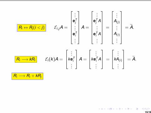
Ri ↔ Rj(i < j) Ei,jA =
...eT
j...
eTi...
A =
...eT
j A...
eTi A...
=
...A(j)
...A(i)
...
= A.
Ri −→ kRi Ei(k)A =
...
keTi
...
A =
...
keTi A...
=
...
kA(i)...
= A.
Ri −→ Ri + kRj
Ei,j(k)A =
...
eTi + keT
j...
A =
...
(eTi + keT
j )A...
=
...
A(i) + kA(j)...
= A.
15/19

Ri ↔ Rj(i < j) Ei,jA =
...eT
j...
eTi...
A =
...eT
j A...
eTi A...
=
...A(j)
...A(i)
...
= A.
Ri −→ kRi Ei(k)A =
...
keTi
...
A =
...
keTi A...
=
...
kA(i)...
= A.
Ri −→ Ri + kRj
Ei,j(k)A =
...
eTi + keT
j...
A =
...
(eTi + keT
j )A...
=
...
A(i) + kA(j)...
= A.
15/19

Ri ↔ Rj(i < j) Ei,jA =
...eT
j...
eTi...
A =
...eT
j A...
eTi A...
=
...A(j)
...A(i)
...
= A.
Ri −→ kRi Ei(k)A =
...
keTi
...
A =
...
keTi A...
=
...
kA(i)...
= A.
Ri −→ Ri + kRj
Ei,j(k)A =
...
eTi + keT
j...
A
=
...
(eTi + keT
j )A...
=
...
A(i) + kA(j)...
= A.
15/19

Ri ↔ Rj(i < j) Ei,jA =
...eT
j...
eTi...
A =
...eT
j A...
eTi A...
=
...A(j)
...A(i)
...
= A.
Ri −→ kRi Ei(k)A =
...
keTi
...
A =
...
keTi A...
=
...
kA(i)...
= A.
Ri −→ Ri + kRj
Ei,j(k)A =
...
eTi + keT
j...
A =
...
(eTi + keT
j )A...
=
...
A(i) + kA(j)...
= A.
15/19
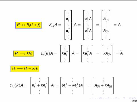
Ri ↔ Rj(i < j) Ei,jA =
...eT
j...
eTi...
A =
...eT
j A...
eTi A...
=
...A(j)
...A(i)
...
= A.
Ri −→ kRi Ei(k)A =
...
keTi
...
A =
...
keTi A...
=
...
kA(i)...
= A.
Ri −→ Ri + kRj
Ei,j(k)A =
...
eTi + keT
j...
A =
...
(eTi + keT
j )A...
=
...
A(i) + kA(j)...
= A.
15/19
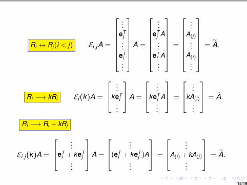
Ri ↔ Rj(i < j) Ei,jA =
...eT
j...
eTi...
A =
...eT
j A...
eTi A...
=
...A(j)
...A(i)
...
= A.
Ri −→ kRi Ei(k)A =
...
keTi
...
A =
...
keTi A...
=
...
kA(i)...
= A.
Ri −→ Ri + kRj
Ei,j(k)A =
...
eTi + keT
j...
A =
...
(eTi + keT
j )A...
=
...
A(i) + kA(j)...
= A.
15/19

Invertibility of Elementary Matrices
The following result is a consequence of the last proposition.Elementary matrices are invertible and the inverses are also el-ementary matrices.
To see this, let E be an elementary matrix. Then E is obtainedfrom I by an elementary row operation. There is clearly an“inverse elementary row operation”, which will transform E backto I. Now if Suppose E is the elementary matrix obtained bymaking this “inverse elementary row operation” on I. Then bythe previous proposition, we see that
EE = I and EE = I.
Thus E is invertible and E−1 is the elementary matrix E .
Exercise : With notation as in the previous slides, show that(i) E−1
i,j = Ei,j , (ii) Ei(k)−1 = Ei(1/k) and (iii) Ei,j(k)−1 = Ei,j(−k).
16/19

Invertibility of Elementary Matrices
The following result is a consequence of the last proposition.Elementary matrices are invertible and the inverses are also el-ementary matrices.
To see this, let E be an elementary matrix. Then E is obtainedfrom I by an elementary row operation. There is clearly an“inverse elementary row operation”, which will transform E backto I. Now if Suppose E is the elementary matrix obtained bymaking this “inverse elementary row operation” on I. Then bythe previous proposition, we see that
EE = I and EE = I.
Thus E is invertible and E−1 is the elementary matrix E .
Exercise : With notation as in the previous slides, show that(i) E−1
i,j
= Ei,j , (ii) Ei(k)−1 = Ei(1/k) and (iii) Ei,j(k)−1 = Ei,j(−k).
16/19

Invertibility of Elementary Matrices
The following result is a consequence of the last proposition.Elementary matrices are invertible and the inverses are also el-ementary matrices.
To see this, let E be an elementary matrix. Then E is obtainedfrom I by an elementary row operation. There is clearly an“inverse elementary row operation”, which will transform E backto I. Now if Suppose E is the elementary matrix obtained bymaking this “inverse elementary row operation” on I. Then bythe previous proposition, we see that
EE = I and EE = I.
Thus E is invertible and E−1 is the elementary matrix E .
Exercise : With notation as in the previous slides, show that(i) E−1
i,j = Ei,j , (ii) Ei(k)−1 = Ei(1/k) and (iii) Ei,j(k)−1 = Ei,j(−k).
16/19

Corollary
CorollaryIf A is an invertible matrix,
then A can be written as a product ofelementary matrices.
Proof : If A is invertible, then the system Ax = b has a uniquesolution, namely x = A−1b, for every b ∈ Rm. Hence thereduced row echelon form of A must be the identity matrix I.Consequently, there are elementary matrices E1, . . . , Ek suchthat Ek . . . E1A = I. This gives A = (Ek . . . E1)
−1 = E−11 . . . E−1
k .
Gauss-Jordan method for finding A−1
Let A be invertible, and suppose Ek . . . E1A = I for someelementary matices E1, . . . , Ek . Then, Ek . . . E1I = A−1.That is, the elementary row operations performed on A toreduce it to identity matrix I, performed in the same order on Ireduces I to A−1. In case the RREF of A is not I, then A is notinvertible.
17/19

Corollary
CorollaryIf A is an invertible matrix, then A can be written as a product ofelementary matrices.
Proof :
If A is invertible, then the system Ax = b has a uniquesolution, namely x = A−1b, for every b ∈ Rm. Hence thereduced row echelon form of A must be the identity matrix I.Consequently, there are elementary matrices E1, . . . , Ek suchthat Ek . . . E1A = I. This gives A = (Ek . . . E1)
−1 = E−11 . . . E−1
k .
Gauss-Jordan method for finding A−1
Let A be invertible, and suppose Ek . . . E1A = I for someelementary matices E1, . . . , Ek . Then, Ek . . . E1I = A−1.That is, the elementary row operations performed on A toreduce it to identity matrix I, performed in the same order on Ireduces I to A−1. In case the RREF of A is not I, then A is notinvertible.
17/19

Corollary
CorollaryIf A is an invertible matrix, then A can be written as a product ofelementary matrices.
Proof : If A is invertible,
then the system Ax = b has a uniquesolution, namely x = A−1b, for every b ∈ Rm. Hence thereduced row echelon form of A must be the identity matrix I.Consequently, there are elementary matrices E1, . . . , Ek suchthat Ek . . . E1A = I. This gives A = (Ek . . . E1)
−1 = E−11 . . . E−1
k .
Gauss-Jordan method for finding A−1
Let A be invertible, and suppose Ek . . . E1A = I for someelementary matices E1, . . . , Ek . Then, Ek . . . E1I = A−1.That is, the elementary row operations performed on A toreduce it to identity matrix I, performed in the same order on Ireduces I to A−1. In case the RREF of A is not I, then A is notinvertible.
17/19

Corollary
CorollaryIf A is an invertible matrix, then A can be written as a product ofelementary matrices.
Proof : If A is invertible, then the system Ax = b has a uniquesolution, namely x = A−1b, for every b ∈ Rm. Hence thereduced row echelon form of A must be the identity matrix I.
Consequently, there are elementary matrices E1, . . . , Ek suchthat Ek . . . E1A = I. This gives A = (Ek . . . E1)
−1 = E−11 . . . E−1
k .
Gauss-Jordan method for finding A−1
Let A be invertible, and suppose Ek . . . E1A = I for someelementary matices E1, . . . , Ek . Then, Ek . . . E1I = A−1.That is, the elementary row operations performed on A toreduce it to identity matrix I, performed in the same order on Ireduces I to A−1. In case the RREF of A is not I, then A is notinvertible.
17/19
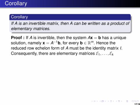
Corollary
CorollaryIf A is an invertible matrix, then A can be written as a product ofelementary matrices.
Proof : If A is invertible, then the system Ax = b has a uniquesolution, namely x = A−1b, for every b ∈ Rm. Hence thereduced row echelon form of A must be the identity matrix I.Consequently, there are elementary matrices E1, . . . , Ek
suchthat Ek . . . E1A = I. This gives A = (Ek . . . E1)
−1 = E−11 . . . E−1
k .
Gauss-Jordan method for finding A−1
Let A be invertible, and suppose Ek . . . E1A = I for someelementary matices E1, . . . , Ek . Then, Ek . . . E1I = A−1.That is, the elementary row operations performed on A toreduce it to identity matrix I, performed in the same order on Ireduces I to A−1. In case the RREF of A is not I, then A is notinvertible.
17/19

Corollary
CorollaryIf A is an invertible matrix, then A can be written as a product ofelementary matrices.
Proof : If A is invertible, then the system Ax = b has a uniquesolution, namely x = A−1b, for every b ∈ Rm. Hence thereduced row echelon form of A must be the identity matrix I.Consequently, there are elementary matrices E1, . . . , Ek suchthat Ek . . . E1A = I.
This gives A = (Ek . . . E1)−1 = E−1
1 . . . E−1k .
Gauss-Jordan method for finding A−1
Let A be invertible, and suppose Ek . . . E1A = I for someelementary matices E1, . . . , Ek . Then, Ek . . . E1I = A−1.That is, the elementary row operations performed on A toreduce it to identity matrix I, performed in the same order on Ireduces I to A−1. In case the RREF of A is not I, then A is notinvertible.
17/19

Corollary
CorollaryIf A is an invertible matrix, then A can be written as a product ofelementary matrices.
Proof : If A is invertible, then the system Ax = b has a uniquesolution, namely x = A−1b, for every b ∈ Rm. Hence thereduced row echelon form of A must be the identity matrix I.Consequently, there are elementary matrices E1, . . . , Ek suchthat Ek . . . E1A = I. This gives A = (Ek . . . E1)
−1 = E−11 . . . E−1
k .
Gauss-Jordan method for finding A−1
Let A be invertible, and suppose Ek . . . E1A = I for someelementary matices E1, . . . , Ek . Then, Ek . . . E1I = A−1.That is, the elementary row operations performed on A toreduce it to identity matrix I, performed in the same order on Ireduces I to A−1. In case the RREF of A is not I, then A is notinvertible.
17/19

Corollary
CorollaryIf A is an invertible matrix, then A can be written as a product ofelementary matrices.
Proof : If A is invertible, then the system Ax = b has a uniquesolution, namely x = A−1b, for every b ∈ Rm. Hence thereduced row echelon form of A must be the identity matrix I.Consequently, there are elementary matrices E1, . . . , Ek suchthat Ek . . . E1A = I. This gives A = (Ek . . . E1)
−1 = E−11 . . . E−1
k .
Gauss-Jordan method for finding A−1
Let A be invertible, and suppose Ek . . . E1A = I for someelementary matices E1, . . . , Ek .
Then, Ek . . . E1I = A−1.That is, the elementary row operations performed on A toreduce it to identity matrix I, performed in the same order on Ireduces I to A−1. In case the RREF of A is not I, then A is notinvertible.
17/19

Corollary
CorollaryIf A is an invertible matrix, then A can be written as a product ofelementary matrices.
Proof : If A is invertible, then the system Ax = b has a uniquesolution, namely x = A−1b, for every b ∈ Rm. Hence thereduced row echelon form of A must be the identity matrix I.Consequently, there are elementary matrices E1, . . . , Ek suchthat Ek . . . E1A = I. This gives A = (Ek . . . E1)
−1 = E−11 . . . E−1
k .
Gauss-Jordan method for finding A−1
Let A be invertible, and suppose Ek . . . E1A = I for someelementary matices E1, . . . , Ek . Then, Ek . . . E1I = A−1.
That is, the elementary row operations performed on A toreduce it to identity matrix I, performed in the same order on Ireduces I to A−1. In case the RREF of A is not I, then A is notinvertible.
17/19

Corollary
CorollaryIf A is an invertible matrix, then A can be written as a product ofelementary matrices.
Proof : If A is invertible, then the system Ax = b has a uniquesolution, namely x = A−1b, for every b ∈ Rm. Hence thereduced row echelon form of A must be the identity matrix I.Consequently, there are elementary matrices E1, . . . , Ek suchthat Ek . . . E1A = I. This gives A = (Ek . . . E1)
−1 = E−11 . . . E−1
k .
Gauss-Jordan method for finding A−1
Let A be invertible, and suppose Ek . . . E1A = I for someelementary matices E1, . . . , Ek . Then, Ek . . . E1I = A−1.That is, the elementary row operations performed on A toreduce it to identity matrix I, performed in the same order on Ireduces I to A−1. In case the RREF of A is not I, then A is notinvertible.
17/19
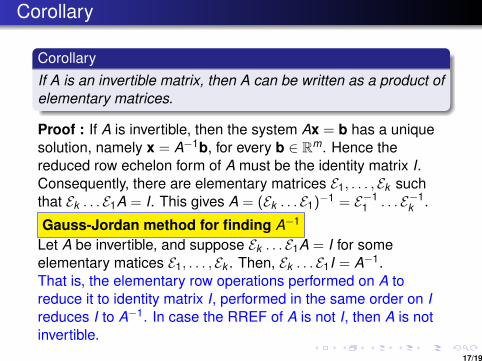
Corollary
CorollaryIf A is an invertible matrix, then A can be written as a product ofelementary matrices.
Proof : If A is invertible, then the system Ax = b has a uniquesolution, namely x = A−1b, for every b ∈ Rm. Hence thereduced row echelon form of A must be the identity matrix I.Consequently, there are elementary matrices E1, . . . , Ek suchthat Ek . . . E1A = I. This gives A = (Ek . . . E1)
−1 = E−11 . . . E−1
k .
Gauss-Jordan method for finding A−1
Let A be invertible, and suppose Ek . . . E1A = I for someelementary matices E1, . . . , Ek . Then, Ek . . . E1I = A−1.That is, the elementary row operations performed on A toreduce it to identity matrix I, performed in the same order on Ireduces I to A−1. In case the RREF of A is not I, then A is notinvertible.
17/19

Inverse of A : an example
[A|I] =
2 1 1
... 1 0 0
4 −6 0... 0 1 0
−2 7 2... 0 0 1
R2→R2+(−2)R1−−−−−−−−−−→R3→R3+(1)R1−−−−−−−−−→
2 1 1
... 1 0 0
0 −8 −2... −2 1 0
0 8 3... 1 0 1
R3→R3+(1)R1−−−−−−−−−→
2 1 1
... 1 0 0
0 −8 −2... −2 1 0
0 0 1... −1 1 1
= [B|L]
This completes the forward elimination. The first half of eliminationhas taken A to echelon form B, and now the second half will take B toI. That is, we create 0′s above the pivots in the last matrix.
18/19
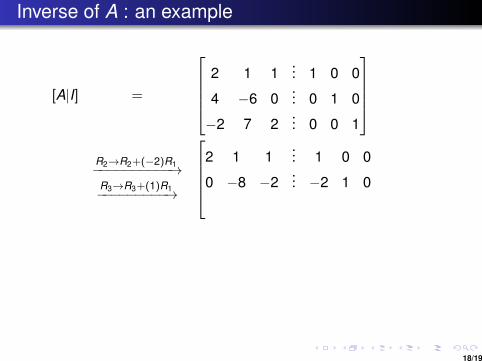
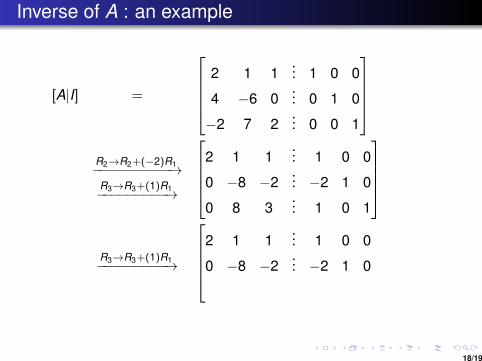

Inverse of A : an example
[A|I] =
2 1 1
... 1 0 0
4 −6 0... 0 1 0
−2 7 2... 0 0 1
R2→R2+(−2)R1−−−−−−−−−−→R3→R3+(1)R1−−−−−−−−−→
2 1 1
... 1 0 0
0 −8 −2... −2 1 0
0 8 3... 1 0 1
R3→R3+(1)R1−−−−−−−−−→
2 1 1
... 1 0 0
0 −8 −2... −2 1 0
0 0 1... −1 1 1
= [B|L]
This completes the forward elimination.
The first half of eliminationhas taken A to echelon form B, and now the second half will take B toI. That is, we create 0′s above the pivots in the last matrix.
18/19

Inverse of A : an example
[A|I] =
2 1 1
... 1 0 0
4 −6 0... 0 1 0
−2 7 2... 0 0 1
R2→R2+(−2)R1−−−−−−−−−−→R3→R3+(1)R1−−−−−−−−−→
2 1 1
... 1 0 0
0 −8 −2... −2 1 0
0 8 3... 1 0 1
R3→R3+(1)R1−−−−−−−−−→
2 1 1
... 1 0 0
0 −8 −2... −2 1 0
0 0 1... −1 1 1
= [B|L]
This completes the forward elimination. The first half of eliminationhas taken A to echelon form B, and now the second half will take B toI.
That is, we create 0′s above the pivots in the last matrix.
18/19

Inverse of A : an example
[A|I] =
2 1 1
... 1 0 0
4 −6 0... 0 1 0
−2 7 2... 0 0 1
R2→R2+(−2)R1−−−−−−−−−−→R3→R3+(1)R1−−−−−−−−−→
2 1 1
... 1 0 0
0 −8 −2... −2 1 0
0 8 3... 1 0 1
R3→R3+(1)R1−−−−−−−−−→
2 1 1
... 1 0 0
0 −8 −2... −2 1 0
0 0 1... −1 1 1
= [B|L]
This completes the forward elimination. The first half of eliminationhas taken A to echelon form B, and now the second half will take B toI. That is, we create 0′s above the pivots in the last matrix. 18/19

Example continued...
[B|L]R2→R2+(2)R3−−−−−−−−−→
R1→R1+(−1)R3−−−−−−−−−−→
2 1 0
... 2 −1 −1
0 −8 0... −4 3 2
0 0 1... −1 1 1
R1→R1+(1/8)R2−−−−−−−−−−→
2 0 0
... 128 −5
8 −68
0 −8 0... −4 3 2
0 0 1... −1 1 1
R1→R1/2−−−−−−→
R2→R2/−8−−−−−−−→
1 0 0
... 1216 − 5
16 − 616
0 1 0... 4
8 −38 −2
8
0 0 1... −1 1 1
= [I|A−1].
19/19
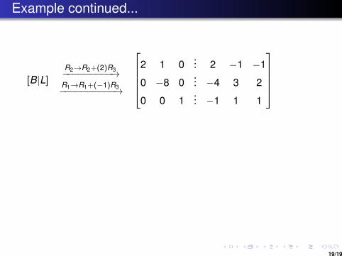

Example continued...
[B|L]R2→R2+(2)R3−−−−−−−−−→
R1→R1+(−1)R3−−−−−−−−−−→
2 1 0
... 2 −1 −1
0 −8 0... −4 3 2
0 0 1... −1 1 1
R1→R1+(1/8)R2−−−−−−−−−−→
2 0 0
... 128 −5
8 −68
0 −8 0... −4 3 2
0 0 1... −1 1 1
R1→R1/2−−−−−−→R2→R2/−8−−−−−−−→
1 0 0
... 1216 − 5
16 − 616
0 1 0... 4
8 −38 −2
8
0 0 1... −1 1 1
= [I|A−1].
19/19

Example continued...
[B|L]R2→R2+(2)R3−−−−−−−−−→
R1→R1+(−1)R3−−−−−−−−−−→
2 1 0
... 2 −1 −1
0 −8 0... −4 3 2
0 0 1... −1 1 1
R1→R1+(1/8)R2−−−−−−−−−−→
2 0 0
... 128 −5
8 −68
0 −8 0... −4 3 2
0 0 1... −1 1 1
R1→R1/2−−−−−−→
R2→R2/−8−−−−−−−→
1 0 0
... 1216 − 5
16 − 616
0 1 0... 4
8 −38 −2
8
0 0 1... −1 1 1
= [I|A−1].
19/19
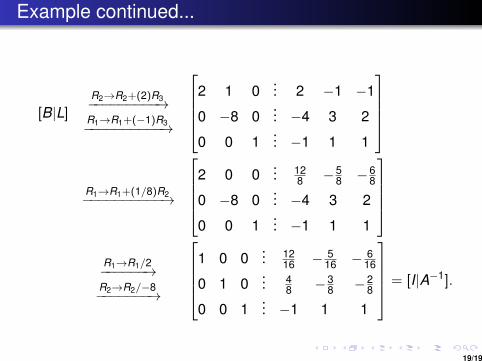
Example continued...
[B|L]R2→R2+(2)R3−−−−−−−−−→
R1→R1+(−1)R3−−−−−−−−−−→
2 1 0
... 2 −1 −1
0 −8 0... −4 3 2
0 0 1... −1 1 1
R1→R1+(1/8)R2−−−−−−−−−−→
2 0 0
... 128 −5
8 −68
0 −8 0... −4 3 2
0 0 1... −1 1 1
R1→R1/2−−−−−−→
R2→R2/−8−−−−−−−→
1 0 0
... 1216 − 5
16 − 616
0 1 0... 4
8 −38 −2
8
0 0 1... −1 1 1
= [I|A−1].
19/19
![Wordnet-Affect [IIT-Bombay]](https://static.fdocuments.net/doc/165x107/55503cebb4c90580748b4770/wordnet-affect-iit-bombay.jpg)