
Stereo - IIT Bombay
67
Stereo CS 763 Ajit Rajwade
Transcript of Stereo - IIT Bombay

Stereo
CS 763
Ajit Rajwade

Contents
• Introduction – stereo in the human eye
• Stereo vision – simplest case
• Epipolar geometry
• Uncalibrated stereo
• Correspondence problem and how to “solve” it
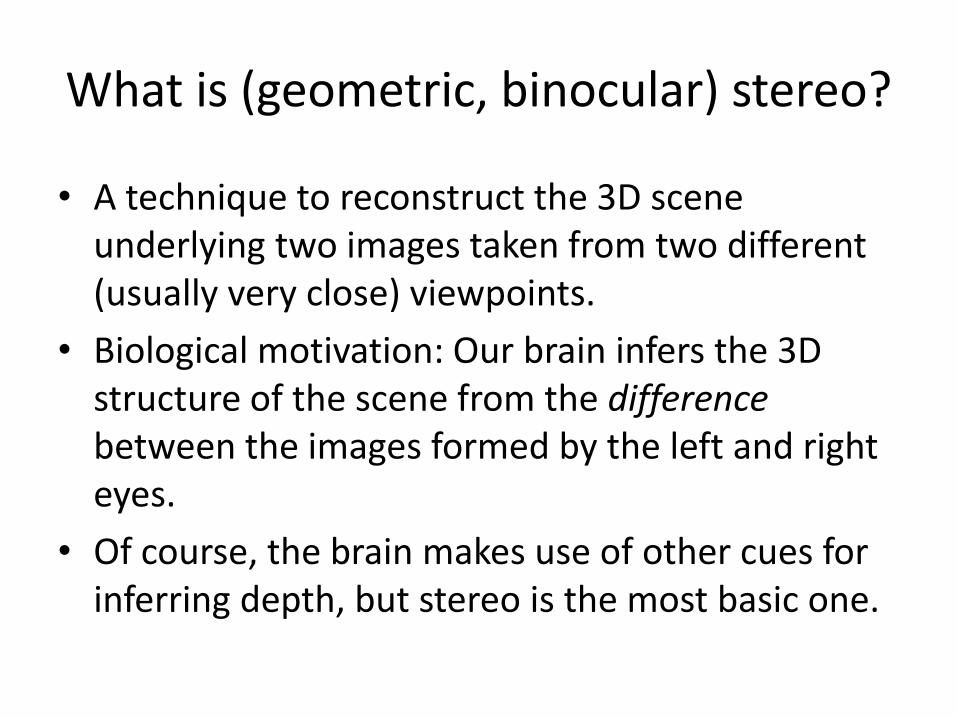
What is (geometric, binocular) stereo?
• A technique to reconstruct the 3D scene underlying two images taken from two different (usually very close) viewpoints.
• Biological motivation: Our brain infers the 3D structure of the scene from the differencebetween the images formed by the left and right eyes.
• Of course, the brain makes use of other cues for inferring depth, but stereo is the most basic one.
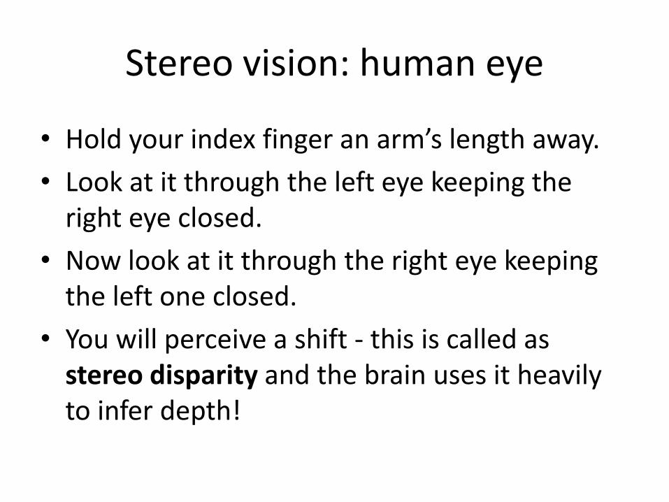
Stereo vision: human eye
• Hold your index finger an arm’s length away.
• Look at it through the left eye keeping the right eye closed.
• Now look at it through the right eye keeping the left one closed.
• You will perceive a shift - this is called as stereo disparity and the brain uses it heavily to infer depth!
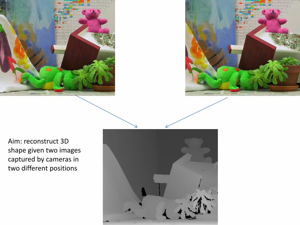
Aim: reconstruct 3D shape given two images captured by cameras in two different positions
Simplest case: stereo
• To perform 3D reconstruction, we must know point correspondences – i.e. given a point in the left image, which is the corresponding point in the right image?
• Let’s make some assumptions about the camera positions!
Simplest case: stereo
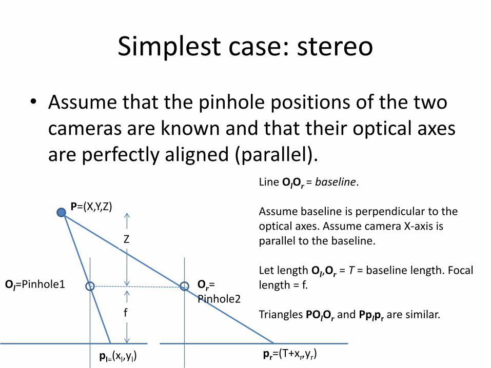
• Assume that the pinhole positions of the two cameras are known and that their optical axes are perfectly aligned (parallel).
P=(X,Y,Z)
Ol=Pinhole1 Or= Pinhole2
pl=(xl,yl) pr=(T+xr,yr)
Line OlOr = baseline.
Assume baseline is perpendicular to the optical axes. Assume camera X-axis is parallel to the baseline.
Let length Ol,Or = T = baseline length. Focal length = f.
Triangles POlOr and Pplpr are similar.
Z
f
Simplest case: stereo
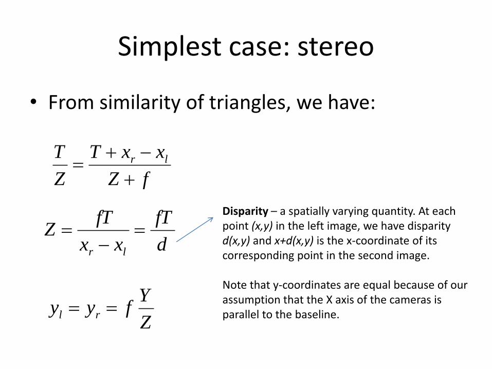
• From similarity of triangles, we have:
fZ
xxT
Z
T lr
d
fT
xx
fTZ
lr
Disparity – a spatially varying quantity. At each point (x,y) in the left image, we have disparity d(x,y) and x+d(x,y) is the x-coordinate of its corresponding point in the second image.
Note that y-coordinates are equal because of our assumption that the X axis of the cameras is parallel to the baseline.
Z
Yfyy rl
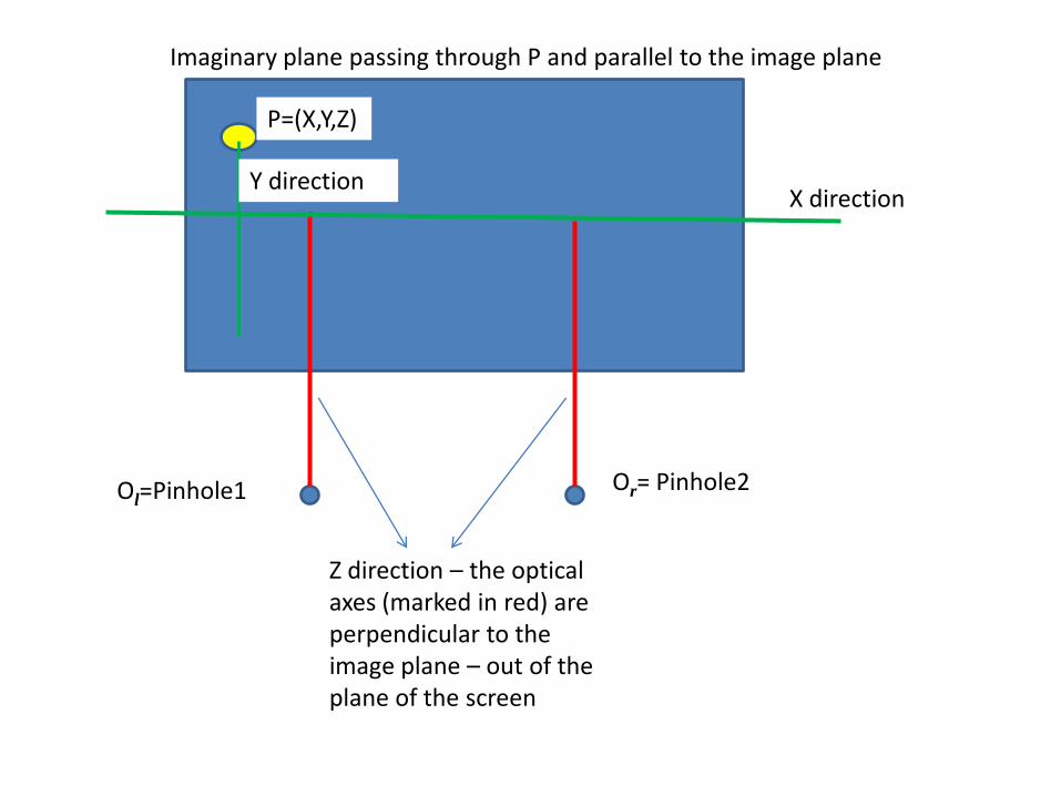
P=(X,Y,Z)
X direction
Z direction – the optical axes (marked in red) are perpendicular to the image plane – out of the plane of the screen
Imaginary plane passing through P and parallel to the image plane
Y direction
Ol=Pinhole1 Or= Pinhole2

Comments
• The search for a point corresponding to one in the left image is restricted to a line parallel to the X axis, as the y-coordinates are the same! This is called the epipolar line.
• A point in the left image may not have a counterpart in the right image (shadows, specularities, occlusions, difference in field of view between the cameras), but if it does, it must lie on the epipolar line.
Comments
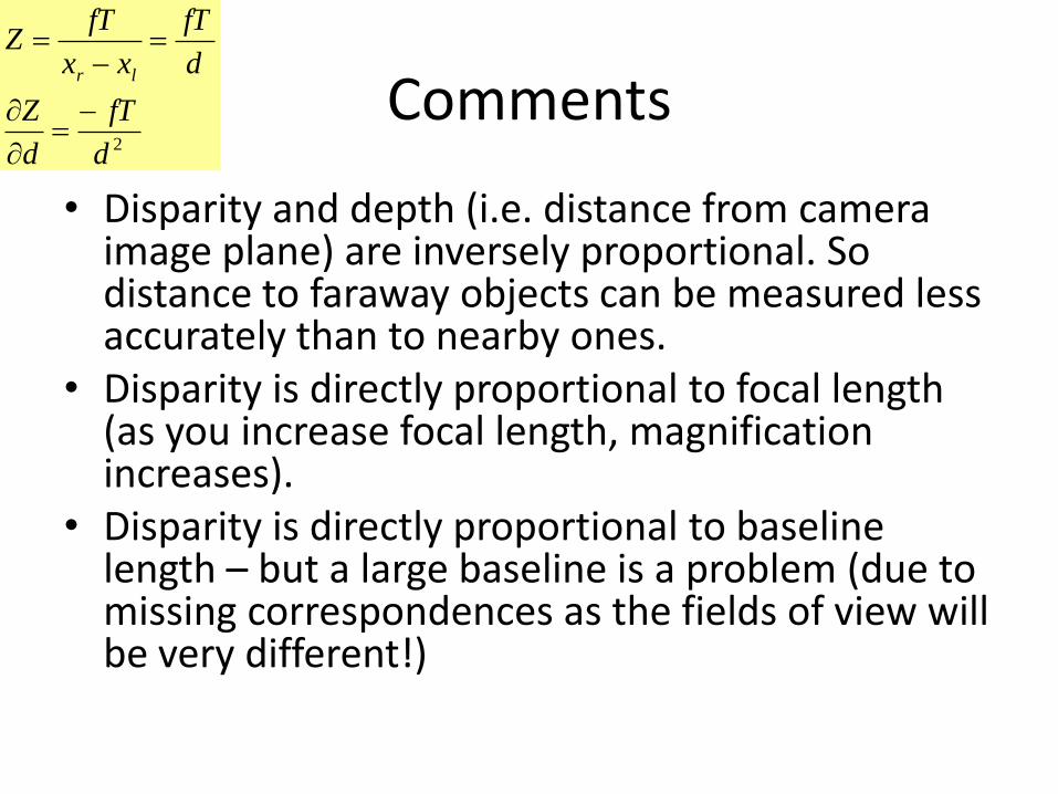
• Disparity and depth (i.e. distance from camera image plane) are inversely proportional. So distance to faraway objects can be measured less accurately than to nearby ones.
• Disparity is directly proportional to focal length (as you increase focal length, magnification increases).
• Disparity is directly proportional to baseline length – but a large baseline is a problem (due to missing correspondences as the fields of view will be very different!)
2d
fT
d
Z
d
fT
xx
fTZ
lr
Two notes of caution
• In most practical stereo systems, it is unreasonable to assume that the optical axes of the two cameras are parallel. We will deal with the case of unaligned cameras on the next bunch of slides.
• Even with parallel optical axes, the correspondence problem is not at all easy! We will deal with this problem later.
Parameters of a stereo system
• Intrinsic parameters – focal lengths, optical centers, camera resolutions
• Extrinsic parameters – rotation and translation to align the coordinate systems of the two cameras.
• The intrinsic or extrinsic parameters or both are often unknown. Stereo reconstruction is essentially a calibration problem!
Epipolar Geometry
• Let’s now study the case where the optical axes of the cameras were not aligned.
• But we will assume full knowledge of camera parameters (intrinsic and extrinsic).
• This is called as fully calibrated stereo.
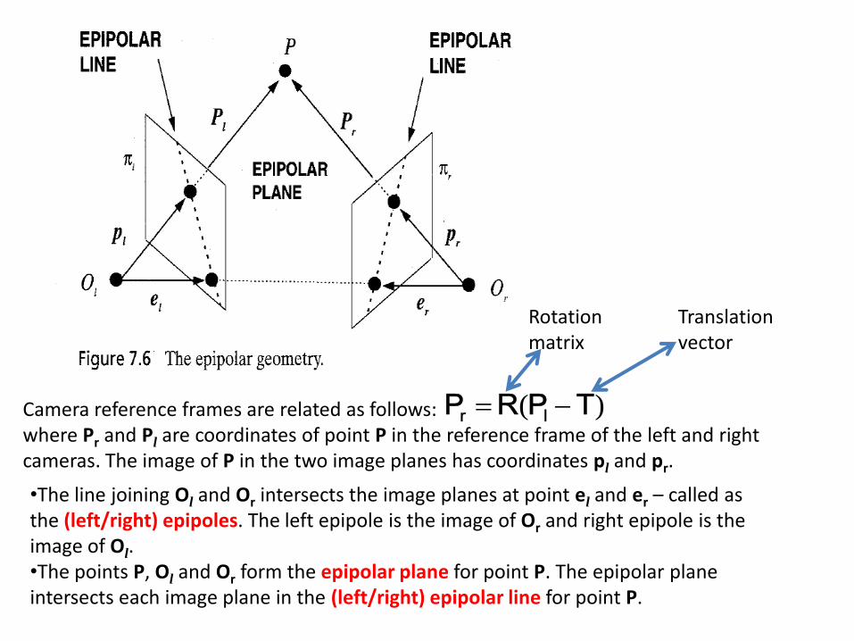
Camera reference frames are related as follows:where Pr and Pl are coordinates of point P in the reference frame of the left and right cameras. The image of P in the two image planes has coordinates pl and pr.
)( TPRP lr
Rotation matrix
Translation vector
•The line joining Ol and Or intersects the image planes at point el and er – called as the (left/right) epipoles. The left epipole is the image of Or and right epipole is the image of Ol. •The points P, Ol and Or form the epipolar plane for point P. The epipolar plane intersects each image plane in the (left/right) epipolar line for point P.

Epipolar Constraint:Given pl, the point P can lie at any point on the line from Ol to pl. The image of ray Ol pl on the right image plane is contained in the right epipolar line (Why? Because Ol, pl and P are collinear – hence their images under perspective projection on the right image plane must also be collinear).
This is called the epipolar constraint. What this means is that the point on the right image plane corresponding to pl (i.e. point pr) is restricted to lie on a single line which happens to be the right epipolar line. All epipolar lines pass through the respective epipoles.
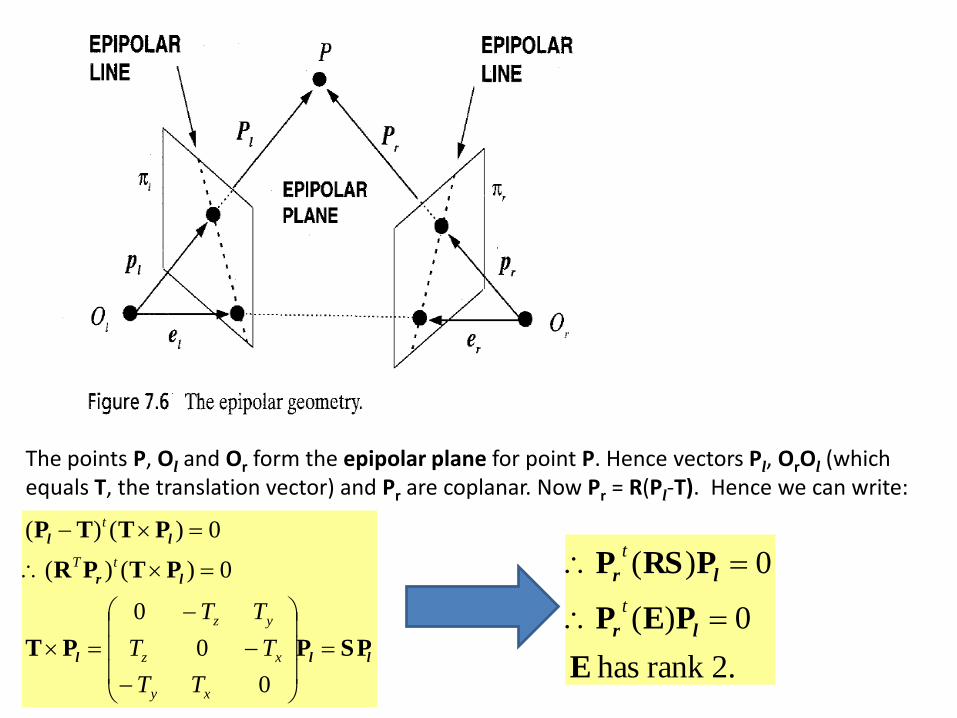
The points P, Ol and Or form the epipolar plane for point P. Hence vectors Pl, OrOl (which equals T, the translation vector) and Pr are coplanar. Now Pr = R(Pl-T). Hence we can write:
lll
lr
ll
SPPPT
PTPR
PTTP
0
0
0
0)()(
0)()(
xy
xz
yz
tT
t
TT
TT
TT
2.rank has
0)(
0)(
E
PEP
PRSP
lr
lr
t
t
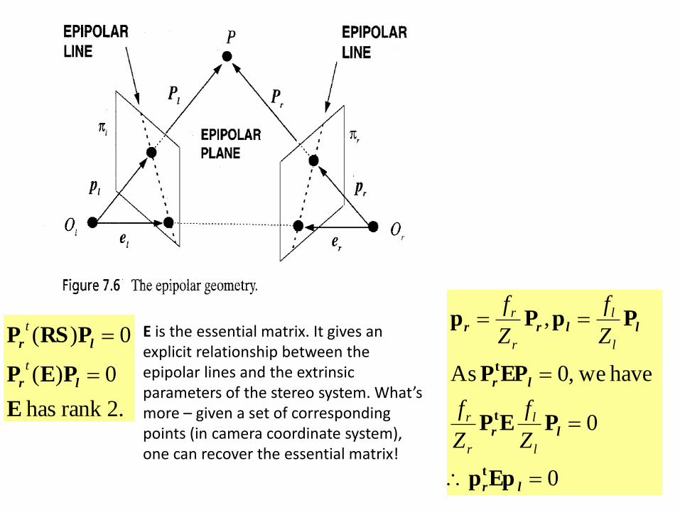
E is the essential matrix. It gives an explicit relationship between the epipolar lines and the extrinsic parameters of the stereo system. What’s more – given a set of corresponding points (in camera coordinate system), one can recover the essential matrix!
0
0
have we,0 As
,
lr
lr
lr
llrr
Epp
PEP
EPP
PpPp
t
t
t
l
l
r
r
l
l
r
r
Z
f
Z
f
Z
f
Z
f
2.rank has
0)(
0)(
E
PEP
PRSP
lr
lr
t
t
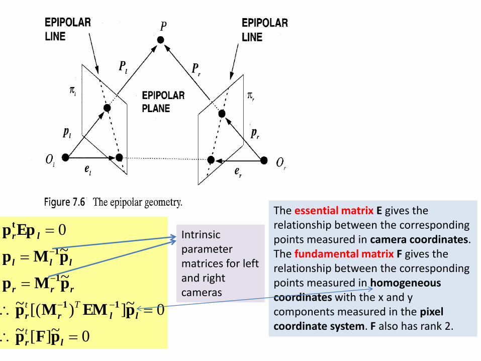
The essential matrix E gives the relationship between the corresponding points measured in camera coordinates. The fundamental matrix F gives the relationship between the corresponding points measured in homogeneous coordinates with the x and y components measured in the pixel coordinate system. F also has rank 2.
0~][~
0~])[(~
~
~
0
lr
llrr
rrr
lll
lr
pFp
pEMMp
pMp
pMp
Epp
11
1
1
t
t
Tt
Intrinsic parameter matrices for left and right cameras
Essential and fundamental matrix
• Consider .
• These equations tell you that given a fixed point pl in the left image, the corresponding point in the right image (i.e. pr) lies on a line (what’s the equation of the line?).
0~][~,0 lrlr pFpEppt t
Determining fundamental and essential matrix
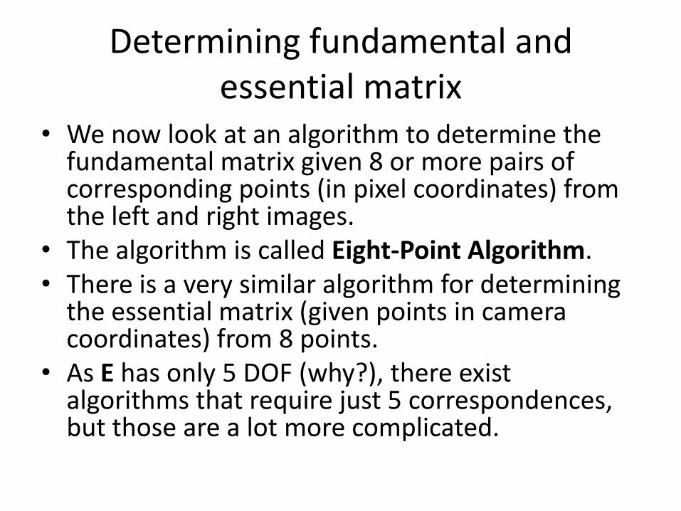
• We now look at an algorithm to determine the fundamental matrix given 8 or more pairs of corresponding points (in pixel coordinates) from the left and right images.
• The algorithm is called Eight-Point Algorithm.• There is a very similar algorithm for determining
the essential matrix (given points in camera coordinates) from 8 points.
• As E has only 5 DOF (why?), there exist algorithms that require just 5 correspondences, but those are a lot more complicated.
Determining fundamental and essential matrix
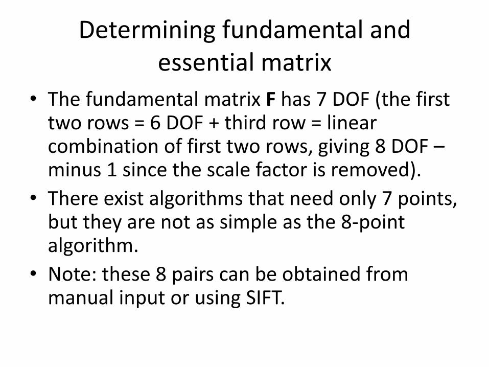
• The fundamental matrix F has 7 DOF (the first two rows = 6 DOF + third row = linear combination of first two rows, giving 8 DOF –minus 1 since the scale factor is removed).
• There exist algorithms that need only 7 points, but they are not as simple as the 8-point algorithm.
• Note: these 8 pairs can be obtained from manual input or using SIFT.

Eight point algorithm
0
Af
pp
pFp
0
0
0
0
0
0
0
0
0
1
..
..
..
..
..
..
1
1
:have we
)1,,(~),1,,(~Let
0~][~,1,
33
32
31
23
22
21
13
12
11
,,,,,,,,,,,,
2,2,2,2,2,2,2,2,2,2,2,2,
1,1,1,1,1,1,1,1,1,1,1,1,
,,,,
F
F
F
F
F
F
F
F
F
yxyyyxyxyxxx
yxyyyxyxyxxx
yxyyyxyxyxxx
yxyx
Nii
NlNlNrNlNrNlNrNrNlNrNlNr
llrlrlrrlrlr
llrlrlrrlrlr
ililirir
t
il,ir,
il,ir,
Eight point algorithm
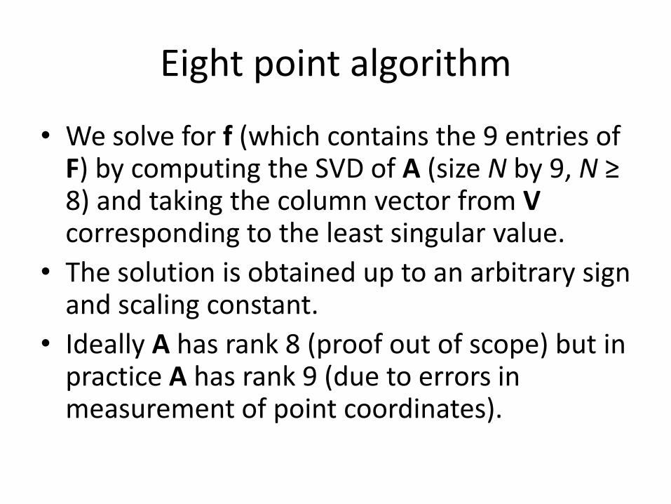
• We solve for f (which contains the 9 entries of F) by computing the SVD of A (size N by 9, N ≥ 8) and taking the column vector from Vcorresponding to the least singular value.
• The solution is obtained up to an arbitrary sign and scaling constant.
• Ideally A has rank 8 (proof out of scope) but in practice A has rank 9 (due to errors in measurement of point coordinates).
Eight point algorithm
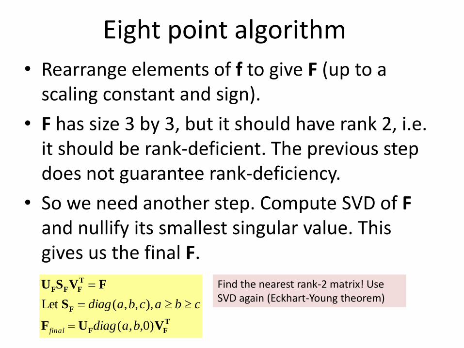
• Rearrange elements of f to give F (up to a scaling constant and sign).
• F has size 3 by 3, but it should have rank 2, i.e. it should be rank-deficient. The previous step does not guarantee rank-deficiency.
• So we need another step. Compute SVD of Fand nullify its smallest singular value. This gives us the final F.
T
FF
F
T
FFF
VUF
S
FVSU
)0,,(
),,,(Let
badiag
cbacbadiag
final
Find the nearest rank-2 matrix! Use SVD again (Eckhart-Young theorem)
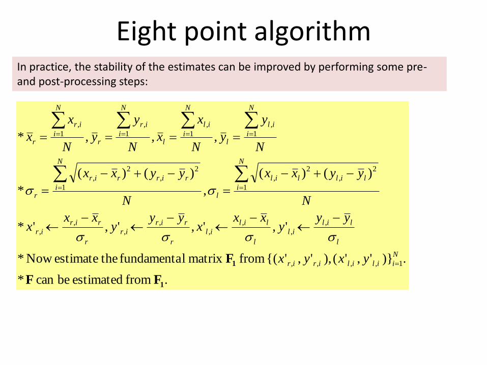
Eight point algorithmIn practice, the stability of the estimates can be improved by performing some pre-and post-processing steps:
. from estimated be can *
.)}','(),','{( frommatrix lfundamenta theestimateNow *
',',','*
)()(
,
)()(
*
,,,*
1,,,,
,
,
,
,
,
,
,
,
1
2
,
2
,
1
2
,
2
,
1
,
1
,
1
,
1
,
1
1
FF
FN
iililirir
l
lil
il
l
lil
il
r
rir
ir
r
rir
ir
N
i
lillil
l
N
i
rirrir
r
N
i
il
l
N
i
il
l
N
i
ir
r
N
i
ir
r
yxyx
yyy
xxx
yyy
xxx
N
yyxx
N
yyxx
N
y
yN
x
xN
y
yN
x
x

Estimating epipoles from F
• The left epipole lies on all epipolar lines in the left image. Hence we can write:
. of nullspace thein lies ~
~0~~
Fe
eF
eFpt
r
l
l
l
0
aluesingular v null toingcorrespond of column ~aluesingular v null toingcorrespond of column~
. of nullspace thein lies ~ Likewise,
Fr
F
T
FFF
r
Ue
Ve
FVSU
Fe
l
T
More about using E or F
• We saw how F can be estimated from 8 pairs of corresponding points.
• Given F, we get the equation for the epipolar line for any point, which will restrict the search space for correspondences along this line (instead of the whole image).
• If the camera instrinsic parameters are known, we can also determine E, and use that to infer Rand T (we will see how this inference is done later).
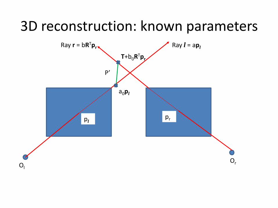
3D reconstruction: known parameters
Ol
Or
Ray l = apl
plpr
P’
Ray r = bRTpr
a0pl
T+b0RTpr
3D reconstruction: known parameters
• The rays r and l may not intersect in practice due to measurement errors.
• Instead we find a line segment s perpendicular to both r and l, with one endpoint on r and another on l.
• Thus we have s lying on the line w = pl x RTpr.
• We treat the midpoint of s as the point of intersection of rays r and l. The midpoint is the point of minimum distance from rays r and l.

3D reconstruction: known parameters
• The concerned segment starts at point a0pl on ray l and ends at point T+b0RTpr on ray r.
• A point on segment s (note that segment s lies on line w) can be expressed as a0pl + c0w = a0pl + c0 (pl x RTpr).
• Hence we have T+b0RTpr = a0 pl + c0 (pl x RTpr). Solve for the coefficients a0,b0,c0.
• Moral of the story: With known camera parameters, 3D reconstruction is essentially unambiguous. Accuracy depends on noise level.
3D reconstruction: only intrinsic parameters are known.
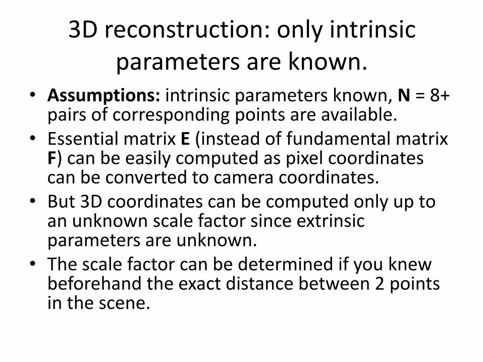
• Assumptions: intrinsic parameters known, N = 8+ pairs of corresponding points are available.
• Essential matrix E (instead of fundamental matrix F) can be easily computed as pixel coordinates can be converted to camera coordinates.
• But 3D coordinates can be computed only up to an unknown scale factor since extrinsic parameters are unknown.
• The scale factor can be determined if you knew beforehand the exact distance between 2 points in the scene.
3D reconstruction: only intrinsic parameters are known.
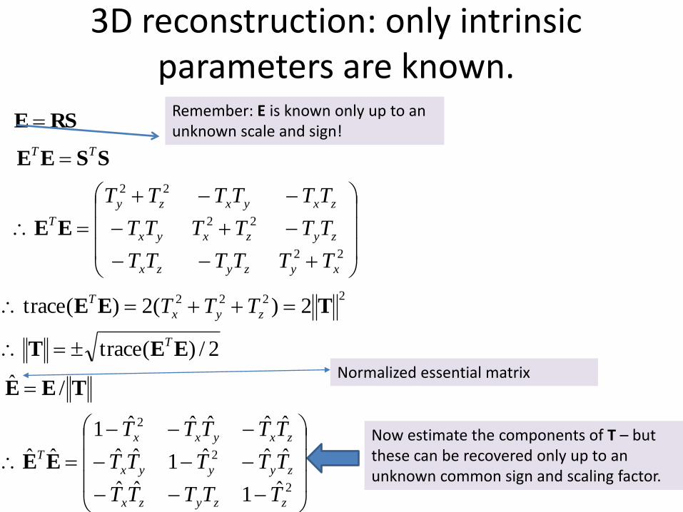
RSE Remember: E is known only up to an unknown scale and sign!
Normalized essential matrix
Now estimate the components of T – but these can be recovered only up to an unknown common sign and scaling factor.
2
2
2
2222
ˆ1ˆˆ
ˆˆˆ1ˆˆ
ˆˆˆˆˆ1
ˆˆ
/ˆ
2/)(trace
2)(2)(trace
zzyzx
zyyyx
zxyxx
T
T
zyx
T
TTTTT
TTTTT
TTTTT
TTT
EE
TEE
EET
TEE
22
22
22
xyzyzx
zyzxyx
zxyxzy
T
TT
TTTTTT
TTTTTT
TTTTTT
EE
SSEE
3D reconstruction: only intrinsic parameters are known.
SRE ˆˆˆ
0ˆˆ
ˆ0ˆ
ˆˆ0
ˆ
xy
xz
yz
TT
TT
TT
S
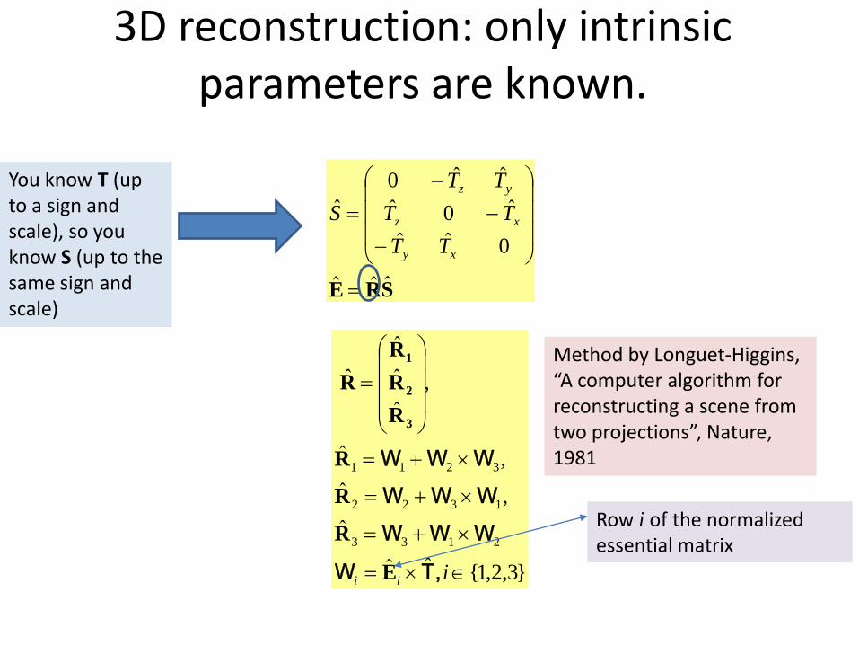
You know T (up to a sign and scale), so you know S (up to the same sign and scale)
}3,2,1{ˆˆ
ˆ
,ˆ
,ˆ
,
ˆ
ˆ
ˆ
ˆ
2133
1322
3211
iii ,TW
WWW
WWW
WWW
E
R
R
R
R
R
R
R
3
2
1 Method by Longuet-Higgins, “A computer algorithm for reconstructing a scene from two projections”, Nature, 1981
Row i of the normalized essential matrix

3D reconstruction: only intrinsic parameters are known.
)ˆ(ˆ,)ˆˆ(
ˆ)ˆˆ(
scale)a (upto hence and scale)a (upto for Solve
31
31 TPRPpRR
TRRr
l
l
T
rr
T
rrll
rl
xf
xffZ
ZZ
)ˆ(ˆ
)ˆ(ˆ
)ˆ(ˆ
)ˆ(ˆ
3
3
TPR
TPRp
TPR
TPRPr
l
lr
l
l
T
T
r
T
r
f
Z
l
l
l
l
f
Z
Z
f
ll
ll
pP
Pp
But
As we know the translation direction only and not its magnitude
Plug in the expression for Pl into the expression for pr and re-arrange to get an expression for Zl
TR ˆˆ
3
l
lT
rf
ZZ lp
3D reconstruction: only intrinsic parameters are known.
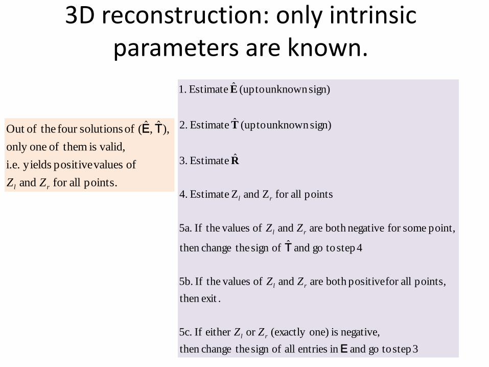
points. allfor and
of valuespositive yieldsi.e.
valid,is themof oneonly
,)ˆ ,ˆ( of solutionsfour theofOut
rl ZZ
TE
3 step togo and in entries all of sign thechange then
negative, is one)(exactly or either If 5c.
.exit then
points, allfor positive both are and of values theIf 5b.
4 step togo and ˆ of sign thechange then
point, somefor negative both are and of values theIf 5a.
points allfor Z and Z Estimate4.
ˆ Estimate3.
sign) unknown (upto ˆ Estimate2.
sign) unknown (uptoˆ Estimate1.
E
T
rl
rl
rl
rl
ZZ
ZZ
ZZ
R
T
E

3D reconstruction: only intrinsic parameters are known.
• To summarize:Our input was a set of N = 8+ corresponding points from two
images taken with cameras of known intrinsic parameters. The extrinsic parameters of the stereo system (i.e. rotation and translation between the optical axes of the two cameras) are unknown.
In such a case, you can estimate only the direction of the baseline vector (i.e. translation direction T) and not its magnitude.
You can estimate the 3D coordinates of the points only up to an unknown scale.
I will once again remind you: we assume correspondences were available or were manually marked. Automated correspondences is not an easy problem, and we will study it soon.
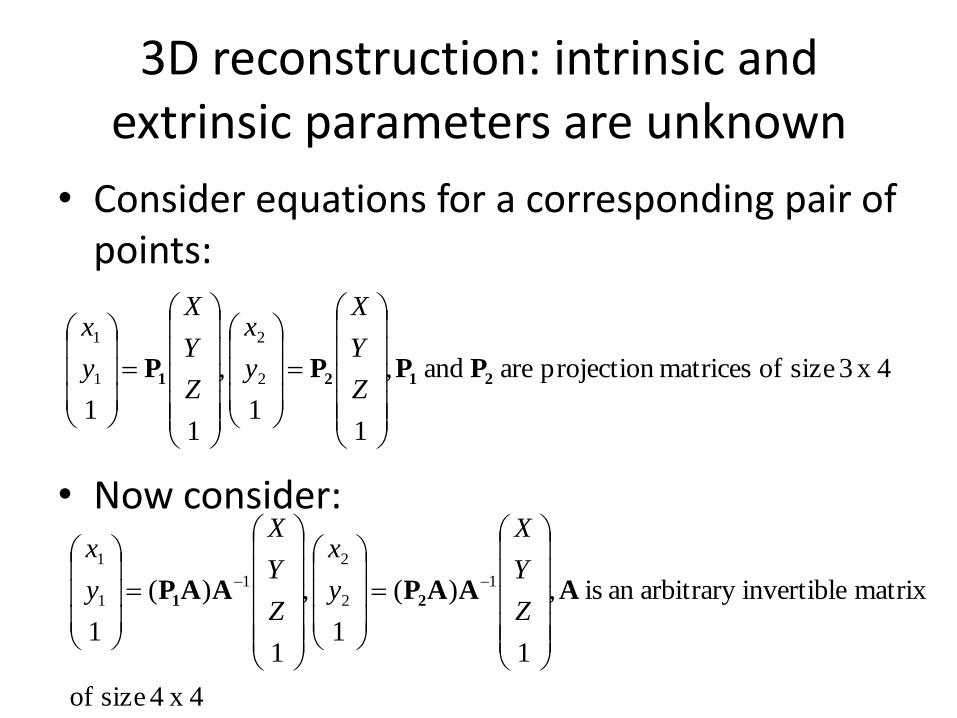
3D reconstruction: intrinsic and extrinsic parameters are unknown
• Consider equations for a corresponding pair of points:
• Now consider:
4x 3 size of matrices projection are and ,
11
,
11
2
2
1
1
2121 PPPP
Z
Y
X
y
x
Z
Y
X
y
x
4x 4 size of
matrix invertiblearbitrary an is ,
1
)(
1
,
1
)(
1
1
2
2
1
1
1
AAAPAAP 21
Z
Y
X
y
x
Z
Y
X
y
x
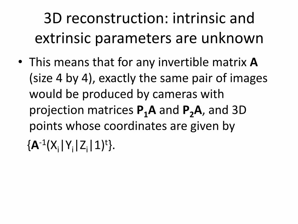
3D reconstruction: intrinsic and extrinsic parameters are unknown
• This means that for any invertible matrix A(size 4 by 4), exactly the same pair of images would be produced by cameras with projection matrices P1A and P2A, and 3D points whose coordinates are given by
{A-1(Xi|Yi|Zi|1)t}.
Correspondence problem
• Several methods:
Correlations/squared difference based methods
Optimization method for inferring the disparity map
Feature-based methods/ Constrained methods – based on dynamic programming
Assumptions
• We will assume the case of coordinate systems of the two cameras being parallel (only a simplification – the method is applicable to the more general case), and their X axes being parallel to the baseline.
• Consider pl = (xl,yl) and pr = (xr,yr) are images of a given point (X,Y,Z) in the two cameras.
• Assume that the gray-levels of corresponding points in the two images are equal.
• So, Il (xl,yl) = Ir(xr,yr).

Assumptions
• Is this brightness constancy assumption valid here?
• Yes, if object is Lambertian.
• Violations: noise, specularity, shadows, occlusion, non-Lambertian surfaces
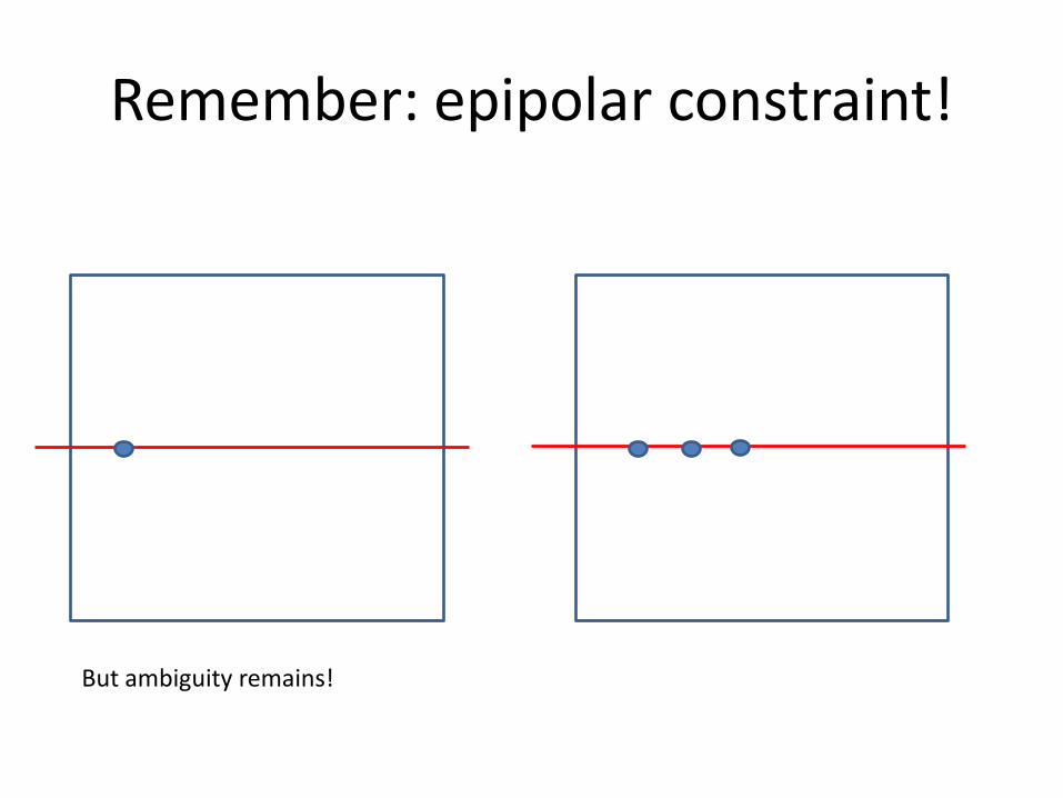
Remember: epipolar constraint!
But ambiguity remains!
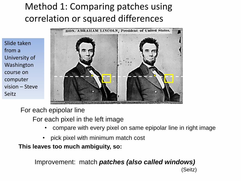
For each epipolar line
For each pixel in the left image
• compare with every pixel on same epipolar line in right image
• pick pixel with minimum match cost
This leaves too much ambiguity, so:
Improvement: match patches (also called windows)(Seitz)
Slide taken from a University of Washington course on computer vision – Steve Seitz
Method 1: Comparing patches using correlation or squared differences
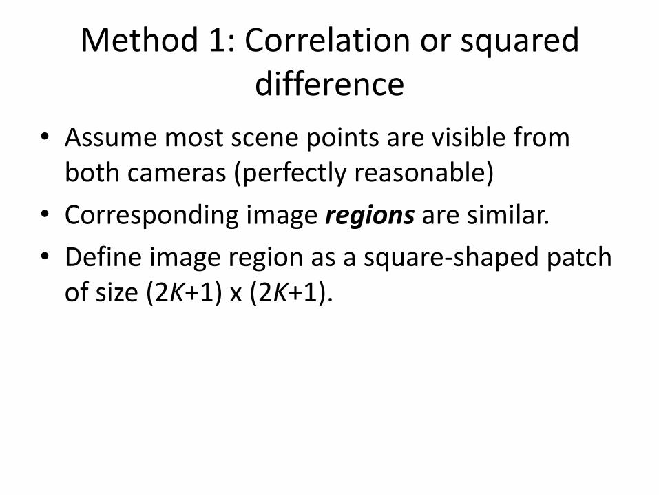
Method 1: Correlation or squared difference
• Assume most scene points are visible from both cameras (perfectly reasonable)
• Corresponding image regions are similar.
• Define image region as a square-shaped patch of size (2K+1) x (2K+1).
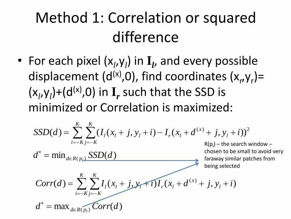
Method 1: Correlation or squared difference
• For each pixel (xl,yl) in Il, and every possible displacement (d(x),0), find coordinates (xr,yr)= (xl,yl)+(d(x),0) in Ir such that the SSD is minimized or Correlation is maximized:
)(min
)),(),(()(
)(
2)(
dSSDd
iyjdxIiyjxIdSSD
lpRd
K
Ki
K
Kj
l
x
lrlll
)(max
),(),()(
)(
)(
dCorrd
iyjdxIiyjxIdCorr
lpRd
K
Ki
K
Kj
l
x
lrlll
R(pl) – the search window –chosen to be small to avoid very faraway similar patches from being selected
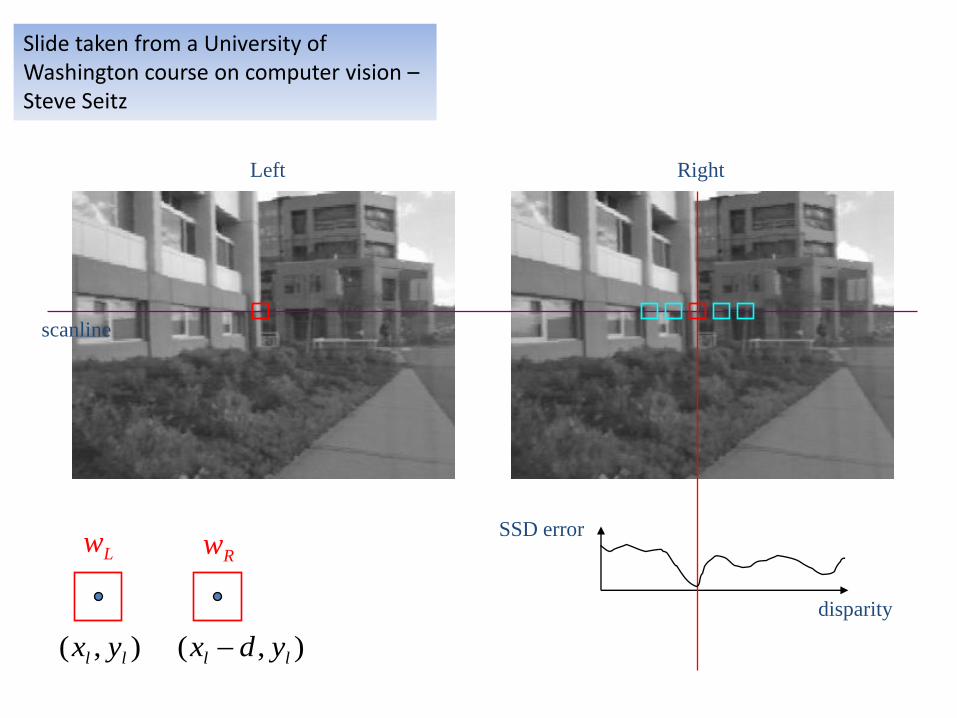
SSD error
disparity
Left Right
scanline
LwRw
),( ll yx ),( ll ydx
Slide taken from a University of Washington course on computer vision –Steve Seitz
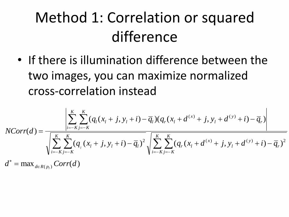
Method 1: Correlation or squared difference
• If there is illumination difference between the two images, you can maximize normalized cross-correlation instead
)(max
)),(()),((
)),()(),((
)(
)(
2)()(2
)()(
dCorrd
qidyjdxqqiyjxq
qidyjdxqqiyjxq
dNCorr
l
l
pRd
K
Ki
K
Kj
r
y
l
x
lrl
K
Ki
K
Kj
ll
K
Ki
K
Kj
r
y
l
x
lrllll
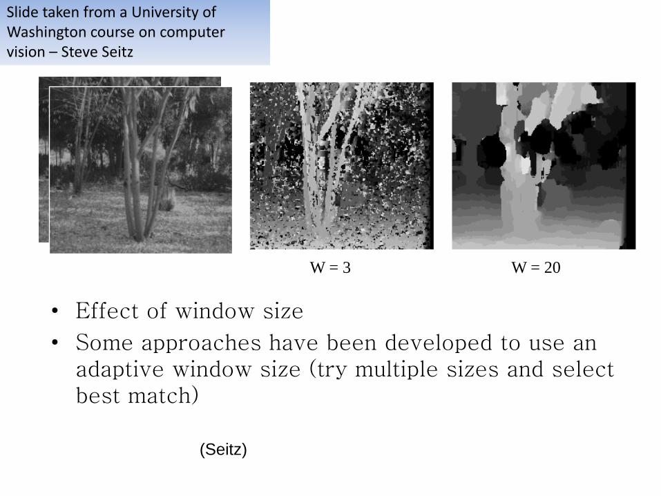
W = 3 W = 20
• Effect of window size
• Some approaches have been developed to use an adaptive window size (try multiple sizes and select best match)
(Seitz)
Slide taken from a University of Washington course on computer vision – Steve Seitz

Method 2: Feature-based methods
• Instead of computing SSD over intensity, compute it over features such as some combination of
(i) image gradient magnitude/orientation
(ii) average/variance of intensity values in a window
• The latter may make the search faster.
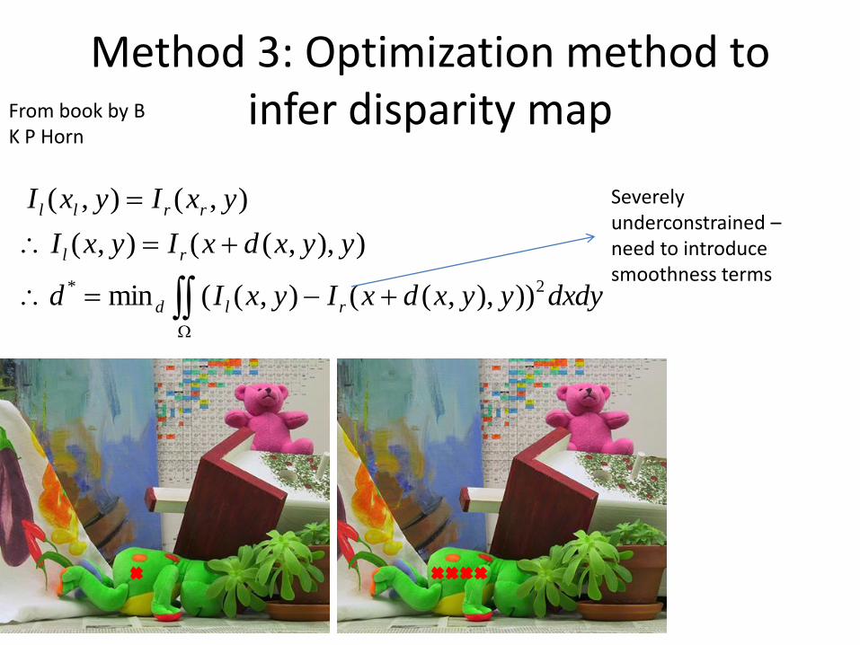
Method 3: Optimization method to infer disparity map
dxdyyyxdxIyxId
yyxdxIyxI
yxIyxI
rld
rl
rrll
2* ))),,((),((min
)),,((),(
),(),( Severelyunderconstrained –need to introduce smoothness terms
From book by B K P Horn
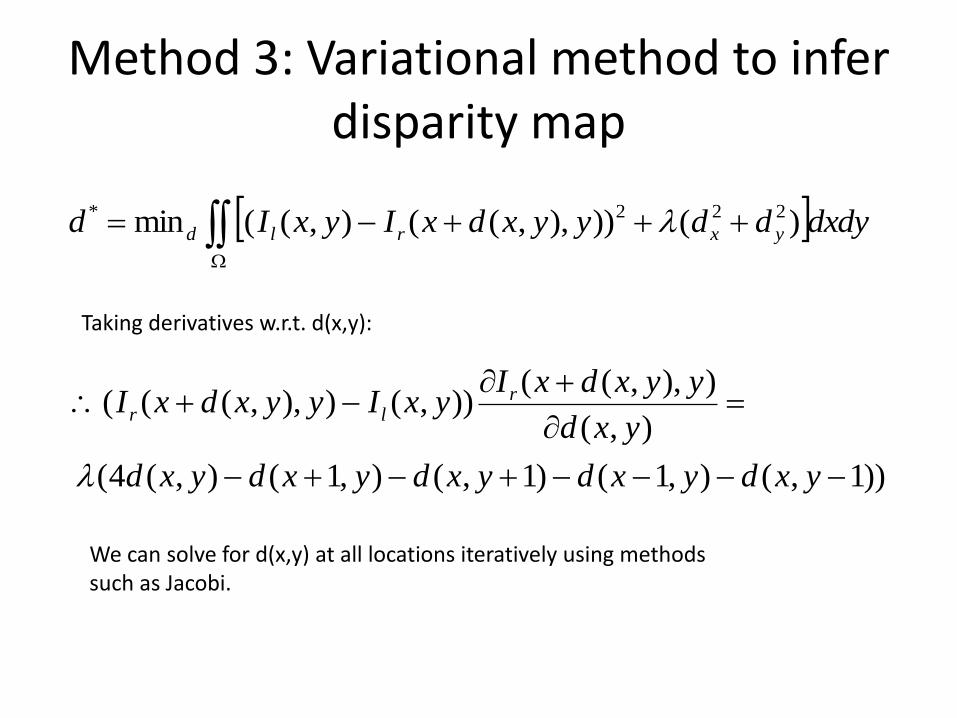
Method 3: Variational method to infer disparity map
dxdyddyyxdxIyxId yxrld )())),,((),((min 222*
))1,(),1()1,(),1(),(4(
),(
)),,(()),()),,(((
yxdyxdyxdyxdyxd
yxd
yyxdxIyxIyyxdxI r
lr
Taking derivatives w.r.t. d(x,y):
We can solve for d(x,y) at all locations iteratively using methods such as Jacobi.
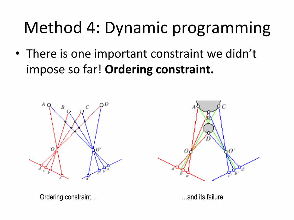
Method 4: Dynamic programming
• There is one important constraint we didn’t impose so far! Ordering constraint.
Ordering constraint… …and its failure
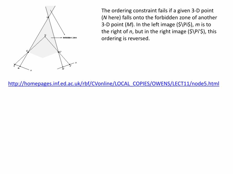
The ordering constraint fails if a given 3-D point (N here) falls onto the forbidden zone of another 3-D point (M). In the left image ($\Pi$), m is to the right of n, but in the right image ($\Pi'$), this ordering is reversed.
http://homepages.inf.ed.ac.uk/rbf/CVonline/LOCAL_COPIES/OWENS/LECT11/node5.html
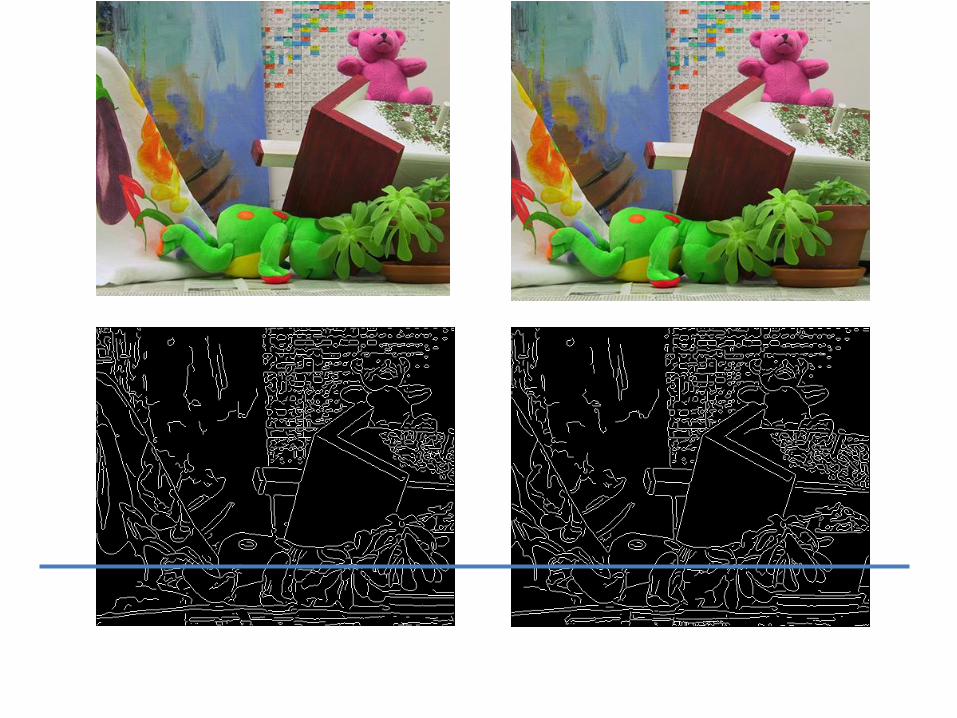
Method 4: Dynamic programming• Step 1: Run an edge detection algorithm on both
images.• Remember: As we assumed parallel optical axes
along Z direction with X-direction baseline, the epipolar lines are horizontal.
• Step 2: For each scanline Ll (epipolar line) in the left image, form a list of edge points. Form a similar list of edge points in the right image on the same scanline (denoted Lr).
• The number of points in these lists may be unequal – let’s denote it as M and N respectively.
Method 4: Dynamic programming• We want to assign nodes from the left list to nodes
in the right one.
• The ordering constraint must be obeyed – if point al
is located before bl on Ll, then ar (the node to which al is assigned) must be located before br (the node to which bl is assigned) on Lr.
• The assignment of correspondences can be framed as a problem of finding a path in a bounded 2D grid with top-left corner at (0,0) and bottom-right corner at (M,N) (see next slide).
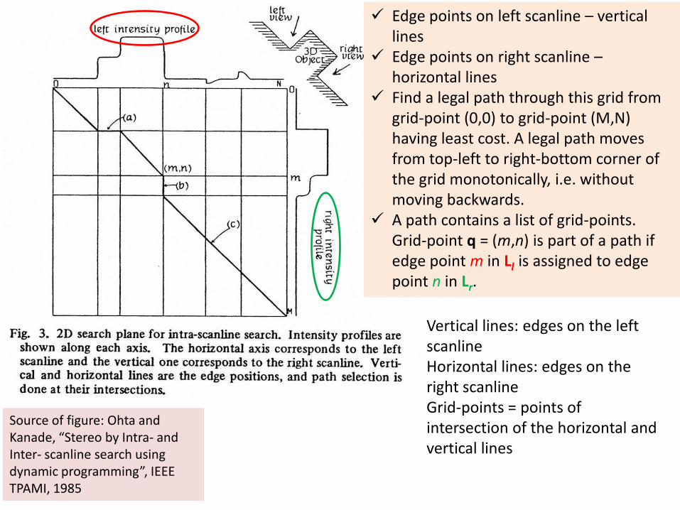
Source of figure: Ohta and Kanade, “Stereo by Intra- and Inter- scanline search using dynamic programming”, IEEE TPAMI, 1985
Edge points on left scanline – vertical lines
Edge points on right scanline –horizontal lines
Find a legal path through this grid from grid-point (0,0) to grid-point (M,N) having least cost. A legal path moves from top-left to right-bottom corner of the grid monotonically, i.e. without moving backwards.
A path contains a list of grid-points. Grid-point q = (m,n) is part of a path if edge point m in Ll is assigned to edge point n in Lr.
Vertical lines: edges on the left scanlineHorizontal lines: edges on the right scanlineGrid-points = points of intersection of the horizontal and vertical lines
Method 4: Dynamic programming
• While searching for correspondence between a pair of edge points, one on Ll (say point pl) and one on Lr (say point pr), the edge points on the left of pl and pr (on Ll and Lr
respectively) should already be processed!
• Start-point and end-point of Ll and Lr are both treated as edge-points for convenience.
Method 4: Dynamic programming
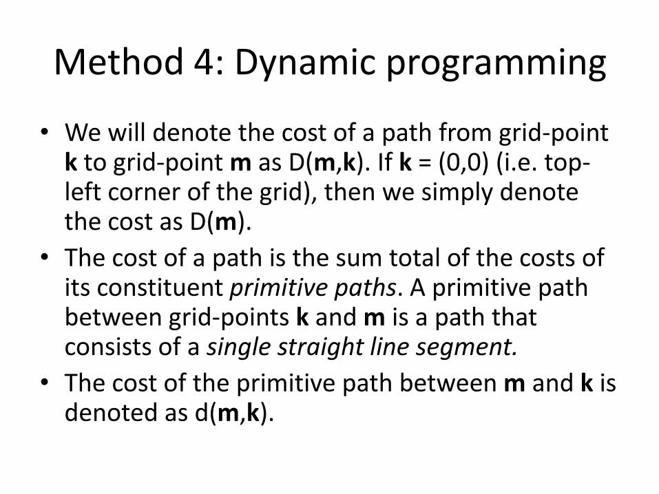
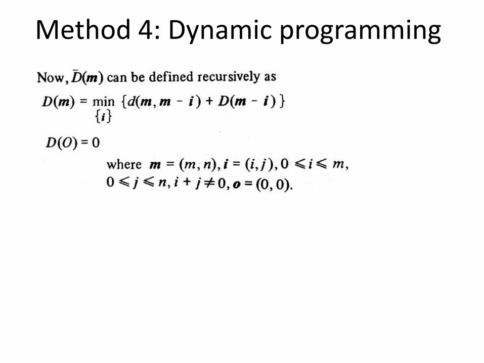
• We will denote the cost of a path from grid-point k to grid-point m as D(m,k). If k = (0,0) (i.e. top-left corner of the grid), then we simply denote the cost as D(m).
• The cost of a path is the sum total of the costs of its constituent primitive paths. A primitive path between grid-points k and m is a path that consists of a single straight line segment.
• The cost of the primitive path between m and k is denoted as d(m,k).
Method 4: Dynamic programming
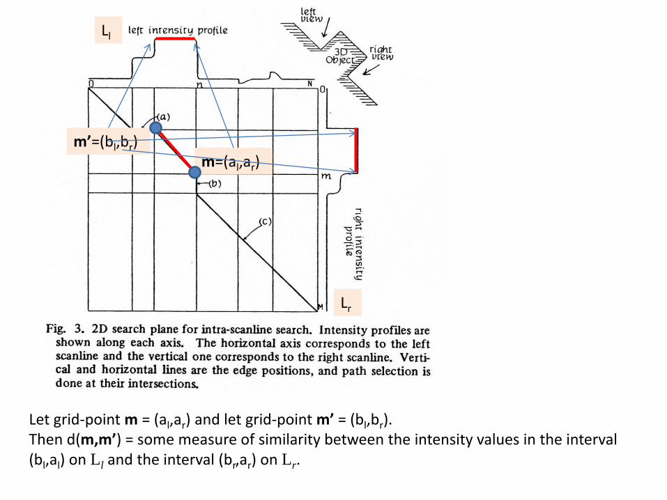
Let grid-point m = (al,ar) and let grid-point m’ = (bl,br).Then d(m,m’) = some measure of similarity between the intensity values in the interval (bl,al) on Ll and the interval (br,ar) on Lr.
Lr
Ll
m=(al,ar)m’=(bl,br)
Method 4: Dynamic programming
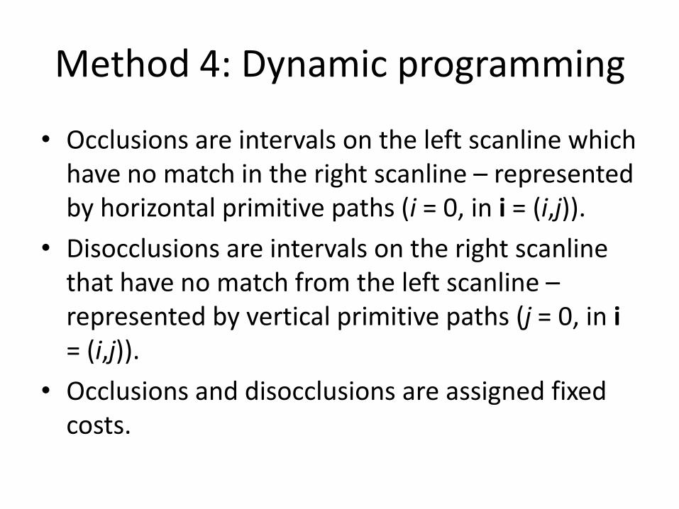
• Occlusions are intervals on the left scanline which have no match in the right scanline – represented by horizontal primitive paths (i = 0, in i = (i,j)).
• Disocclusions are intervals on the right scanlinethat have no match from the left scanline –represented by vertical primitive paths (j = 0, in i= (i,j)).
• Occlusions and disocclusions are assigned fixed costs.
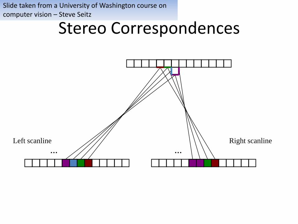
Stereo Correspondences
… …
Left scanline Right scanline
Slide taken from a University of Washington course on computer vision – Steve Seitz
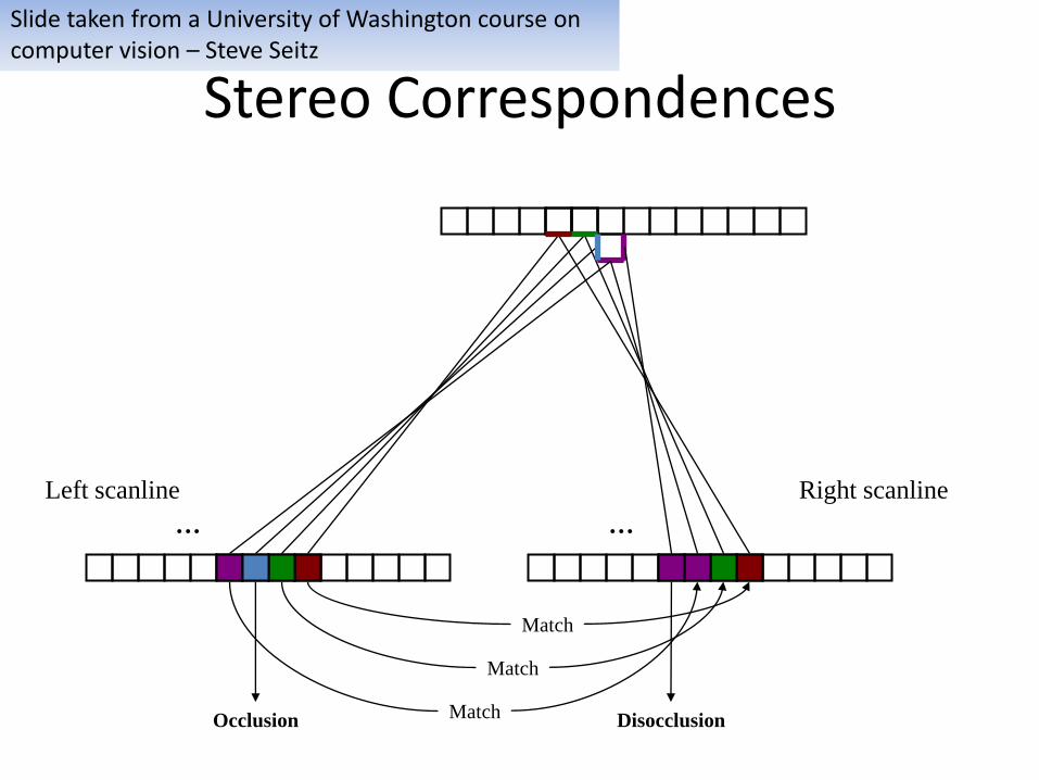
Stereo Correspondences
… …
Left scanline Right scanline
Match
Match
MatchOcclusion Disocclusion
Slide taken from a University of Washington course on computer vision – Steve Seitz

Search Over Correspondences
Three cases:
–Sequential – add cost of match (small if intensities agree)
–Occluded – add cost of no match (large cost)
–Disoccluded – add cost of no match (large cost)
Left scanline
Right scanline
Occluded Pixels
Disoccluded Pixels
Slide taken from a University of Washington course on computer vision – Steve Seitz
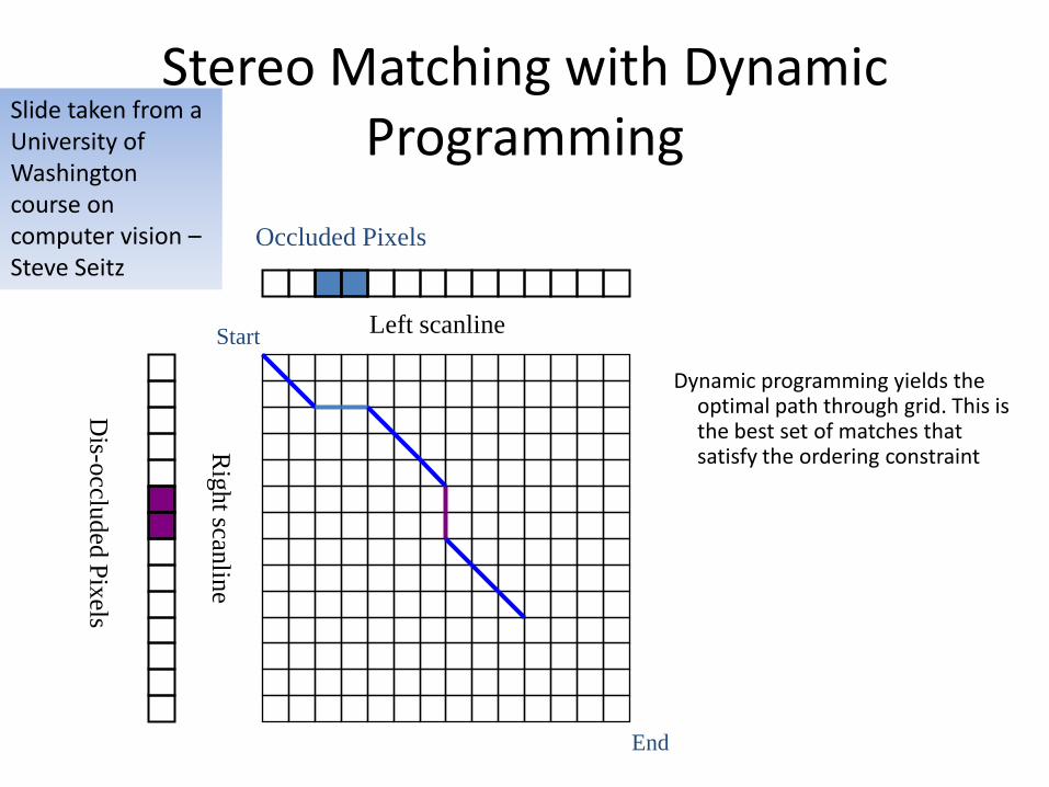
Stereo Matching with Dynamic Programming
Dynamic programming yields the optimal path through grid. This is the best set of matches that satisfy the ordering constraint
Occluded Pixels
Left scanline
Dis-o
ccluded
Pix
els
Rig
ht scan
line
Start
End
Slide taken from a University of Washington course on computer vision –Steve Seitz


![Sentiwordnet [IIT-Bombay]](https://static.fdocuments.net/doc/165x107/54b6d3b14a79594d158b45eb/sentiwordnet-iit-bombay.jpg)