M 8. The Michelson Interferometer - UZH -...

8. The Michelson Interferometer

M

8.1 Introduction

Interference patterns from superposed coherent waves may be used for precise determination of

wavelength or, if the wavelength is known, time-of-flight, path length or other optical parameters

(cf. labs I, Spm and MW). In the present experiment the Michelson Interferometer will be used to

determine the refractive index of air.

Some safety considerations: The interferometer is a delicate instrument and should be handled with

great care. Remove the plastic protection only for adjustment, and put it back in place before any

measurements are made. Never expose your eyes to the light of the mercury lamp, neither directly

nor through the instrument. Never touch any optical components, in particular not the mirrors.

8.2 Theory

a) The Michelson Interferometer

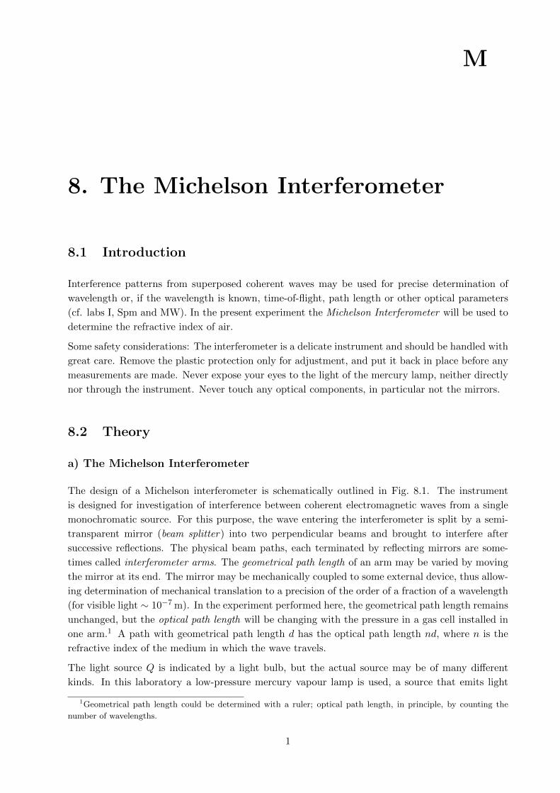
The design of a Michelson interferometer is schematically outlined in Fig. 8.1. The instrument

is designed for investigation of interference between coherent electromagnetic waves from a single

monochromatic source. For this purpose, the wave entering the interferometer is split by a semi-

transparent mirror (beam splitter) into two perpendicular beams and brought to interfere after

successive reflections. The physical beam paths, each terminated by reflecting mirrors are some-

times called interferometer arms. The geometrical path length of an arm may be varied by moving

the mirror at its end. The mirror may be mechanically coupled to some external device, thus allow-

ing determination of mechanical translation to a precision of the order of a fraction of a wavelength

(for visible light ∼ 10−7 m). In the experiment performed here, the geometrical path length remains

unchanged, but the optical path length will be changing with the pressure in a gas cell installed in

one arm.1 A path with geometrical path length d has the optical path length nd, where n is the

refractive index of the medium in which the wave travels.

The light source Q is indicated by a light bulb, but the actual source may be of many different

kinds. In this laboratory a low-pressure mercury vapour lamp is used, a source that emits light

1Geometrical path length could be determined with a ruler; optical path length, in principle, by counting the

number of wavelengths.

1

2 8. The Michelson Interferometer

G : beamsplitter

F M S1 and S2 : mirrors

Q : light source

M : diffusor

G’ : glass plate

F : filter

Q

S1

S2

G’

G

G

d1

d2

Figure 8.1: Principles of the Michelson interferometer (plane view).

only at discrete, well defined wavelengths. A filter F is employed to suppress light of wavelengths

other than the green line of the mercury spectrum. Further requirements on the source that will

not be discussed in detail here, is that of spatial coherence, meaning that the wave entering the

interferometer must retain a constant phase relation (one might think in terms of wave fronts) over

the cross section of the beam, which in practice may be achieved using an entrance collimator (small

hole or slit). The wave must also posses temporal coherence, requiring the source to be phase stable

for a period of time (the coherence time) at least as long as it takes the wave to travel a distance

of the order of the difference in optical length of the interferometer arms. The coherence time is

related to the more familiar notion coherence length through the speed of light in the medium. One

might think of the source as emitting coherent wave trains of the same extension as the coherence

length. The mercury lamp emits light with good coherence.

A beam from the light source is incident on the glass plate G, which is coated on the side seen

from mirror S1 with a thin layer of chromel.2 making it a semitransparent mirror, here employed

as beam splitter. About half of the intensity of the incident light is reflected from the metal layer

of plate G in the direction of mirror S2, then returned and passed through the glass plate G to the

observer. The part of the incident light not reflected in G is transmitted through the plate and

the metal coating, reflected at mirror S1 and returned back to G, where it is reflected by the metal

layer towards the observer and the two beams interfere.

Between plate G and mirror S1 the wave travels twice through a second glass plate G′, the com-

pensator, which to optical precision has the same orientation, the same thickness, and is made of

the same quality of glass as used for plate G but without a metal coating. The compensator, as the

name suggests, compensates for the difference in optical path length between the two beams of the

interferometer that occurs because the beam reflected to mirror S2 passes three times through the

optically denser medium of the glass plate G, whereas the beam transmitted to mirror S1 passes

only once (cf. insert of Figure 8.1 and note that the silver coating on G is facing mirror S1).

2An alloy consisting mainly of nickel and a small part of chromium.

Laboratory Manuals for Physics Majors - Physics PHY112

8.2. THEORY 3

With correct compensation for any optical path difference that relates to the design of the in-

strumental, it suffices to make calculations on the observed changes in the interference pattern to

extract information about e.g. a transverse motion of one mirror or a change in refractive index in

one of the beams.

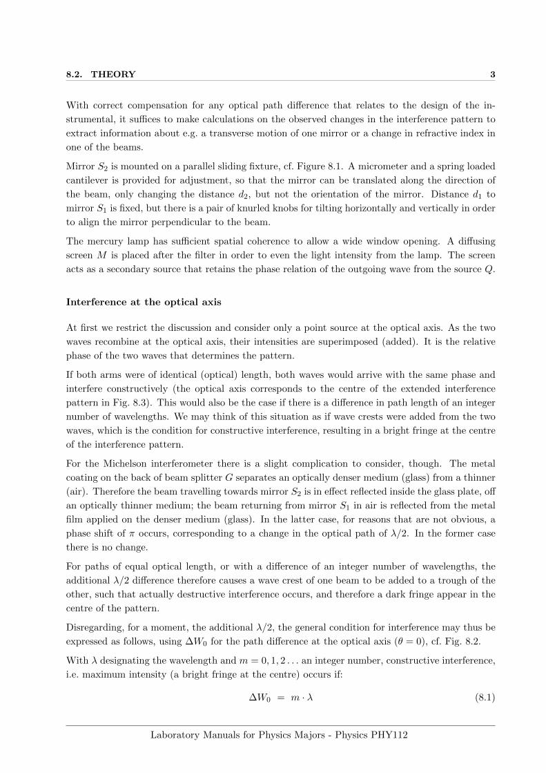
Mirror S2 is mounted on a parallel sliding fixture, cf. Figure 8.1. A micrometer and a spring loaded

cantilever is provided for adjustment, so that the mirror can be translated along the direction of

the beam, only changing the distance d2, but not the orientation of the mirror. Distance d1 to

mirror S1 is fixed, but there is a pair of knurled knobs for tilting horizontally and vertically in order

to align the mirror perpendicular to the beam.

The mercury lamp has sufficient spatial coherence to allow a wide window opening. A diffusing

screen M is placed after the filter in order to even the light intensity from the lamp. The screen

acts as a secondary source that retains the phase relation of the outgoing wave from the source Q.

Interference at the optical axis

At first we restrict the discussion and consider only a point source at the optical axis. As the two

waves recombine at the optical axis, their intensities are superimposed (added). It is the relative

phase of the two waves that determines the pattern.

If both arms were of identical (optical) length, both waves would arrive with the same phase and

interfere constructively (the optical axis corresponds to the centre of the extended interference

pattern in Fig. 8.3). This would also be the case if there is a difference in path length of an integer

number of wavelengths. We may think of this situation as if wave crests were added from the two

waves, which is the condition for constructive interference, resulting in a bright fringe at the centre

of the interference pattern.

For the Michelson interferometer there is a slight complication to consider, though. The metal

coating on the back of beam splitter G separates an optically denser medium (glass) from a thinner

(air). Therefore the beam travelling towards mirror S2 is in effect reflected inside the glass plate, off

an optically thinner medium; the beam returning from mirror S1 in air is reflected from the metal

film applied on the denser medium (glass). In the latter case, for reasons that are not obvious, a

phase shift of π occurs, corresponding to a change in the optical path of λ/2. In the former case

there is no change.

For paths of equal optical length, or with a difference of an integer number of wavelengths, the

additional λ/2 difference therefore causes a wave crest of one beam to be added to a trough of the

other, such that actually destructive interference occurs, and therefore a dark fringe appear in the

centre of the pattern.

Disregarding, for a moment, the additional λ/2, the general condition for interference may thus be

expressed as follows, using ∆W0 for the path difference at the optical axis (θ = 0), cf. Fig. 8.2.

With λ designating the wavelength and m = 0, 1, 2 . . . an integer number, constructive interference,

i.e. maximum intensity (a bright fringe at the centre) occurs if:

∆W0 = m · λ (8.1)



ΔW0 Q2Q1

θ

S S

S

1 2

2

QM

M

θΔWθ

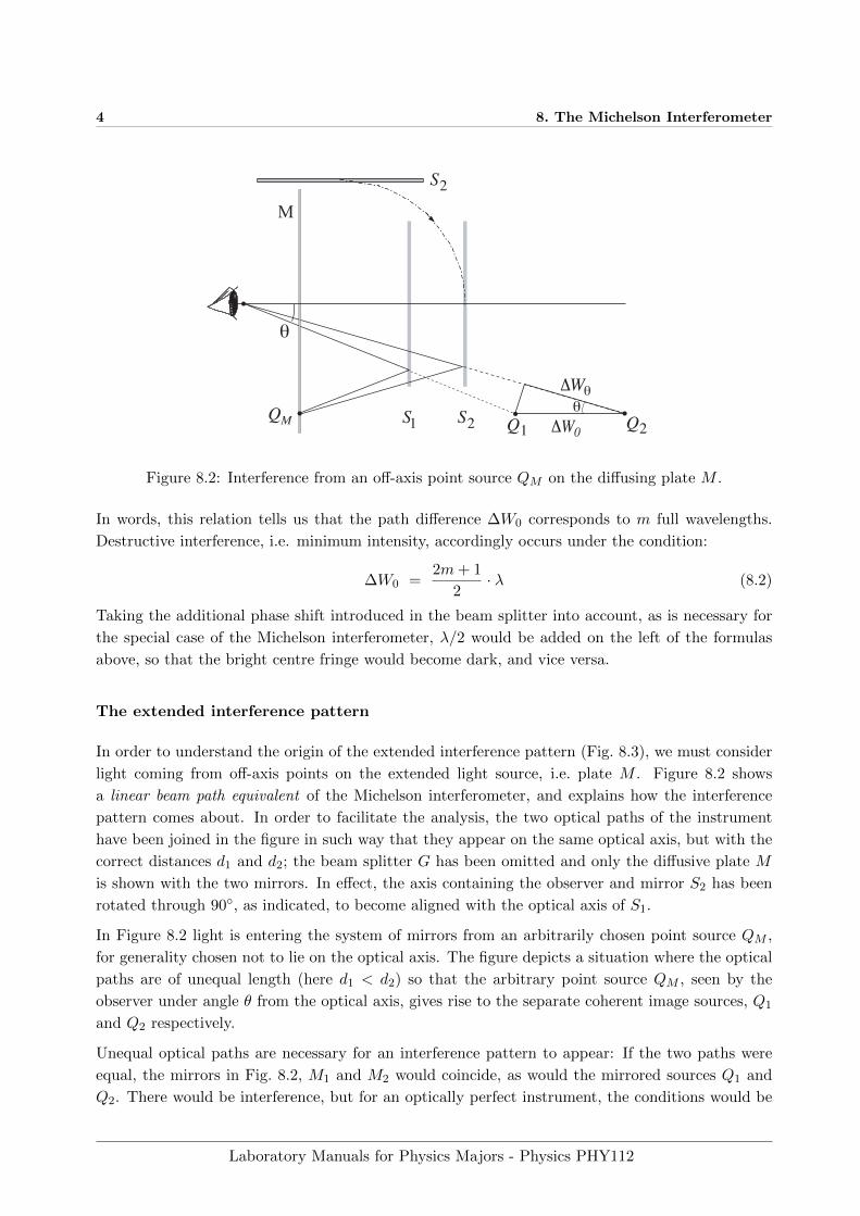
Figure 8.2: Interference from an off-axis point source QM on the diffusing plate M .

In words, this relation tells us that the path difference ∆W0 corresponds to m full wavelengths.

Destructive interference, i.e. minimum intensity, accordingly occurs under the condition:

∆W0 =2m+ 1

2· λ (8.2)

Taking the additional phase shift introduced in the beam splitter into account, as is necessary for

the special case of the Michelson interferometer, λ/2 would be added on the left of the formulas

above, so that the bright centre fringe would become dark, and vice versa.

The extended interference pattern

In order to understand the origin of the extended interference pattern (Fig. 8.3), we must consider

light coming from off-axis points on the extended light source, i.e. plate M . Figure 8.2 shows

a linear beam path equivalent of the Michelson interferometer, and explains how the interference

pattern comes about. In order to facilitate the analysis, the two optical paths of the instrument

have been joined in the figure in such way that they appear on the same optical axis, but with the

correct distances d1 and d2; the beam splitter G has been omitted and only the diffusive plate M

is shown with the two mirrors. In effect, the axis containing the observer and mirror S2 has been

rotated through 90◦, as indicated, to become aligned with the optical axis of S1.

In Figure 8.2 light is entering the system of mirrors from an arbitrarily chosen point source QM ,

for generality chosen not to lie on the optical axis. The figure depicts a situation where the optical

paths are of unequal length (here d1 < d2) so that the arbitrary point source QM , seen by the

observer under angle θ from the optical axis, gives rise to the separate coherent image sources, Q1

and Q2 respectively.

Unequal optical paths are necessary for an interference pattern to appear: If the two paths were

equal, the mirrors in Fig. 8.2, M1 and M2 would coincide, as would the mirrored sources Q1 and

Q2. There would be interference, but for an optically perfect instrument, the conditions would be


8.2. THEORY 5

the same on the optical axis as in all directions θ viewed by the observer, resulting in a degenerate

pattern that covers the entire field of view with the same intensity (in practice this does rarely

occur because of imperfections in the optical components).

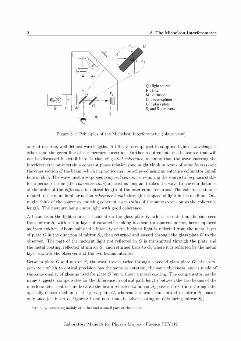
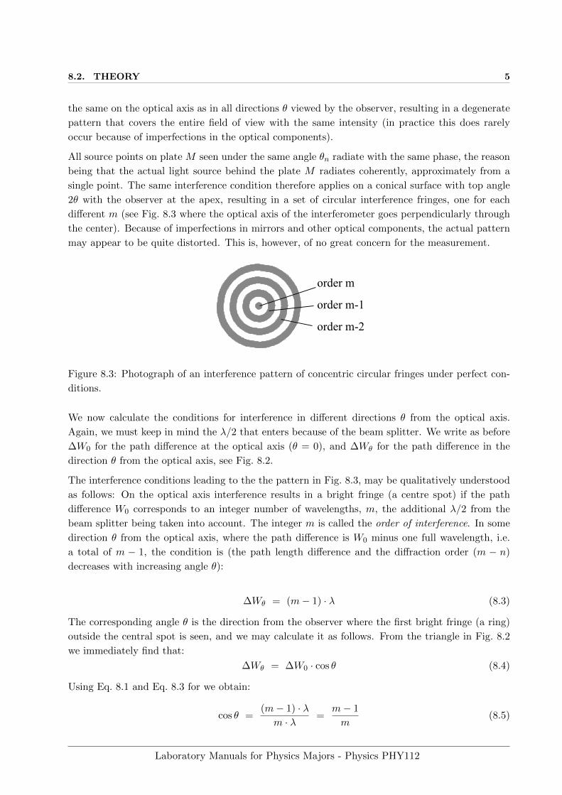
All source points on plate M seen under the same angle θn radiate with the same phase, the reason

being that the actual light source behind the plate M radiates coherently, approximately from a

single point. The same interference condition therefore applies on a conical surface with top angle

2θ with the observer at the apex, resulting in a set of circular interference fringes, one for each

different m (see Fig. 8.3 where the optical axis of the interferometer goes perpendicularly through

the center). Because of imperfections in mirrors and other optical components, the actual pattern

may appear to be quite distorted. This is, however, of no great concern for the measurement.

order m

order m-1

order m-2

Figure 8.3: Photograph of an interference pattern of concentric circular fringes under perfect con-

ditions.

We now calculate the conditions for interference in different directions θ from the optical axis.

Again, we must keep in mind the λ/2 that enters because of the beam splitter. We write as before

∆W0 for the path difference at the optical axis (θ = 0), and ∆Wθ for the path difference in the

direction θ from the optical axis, see Fig. 8.2.

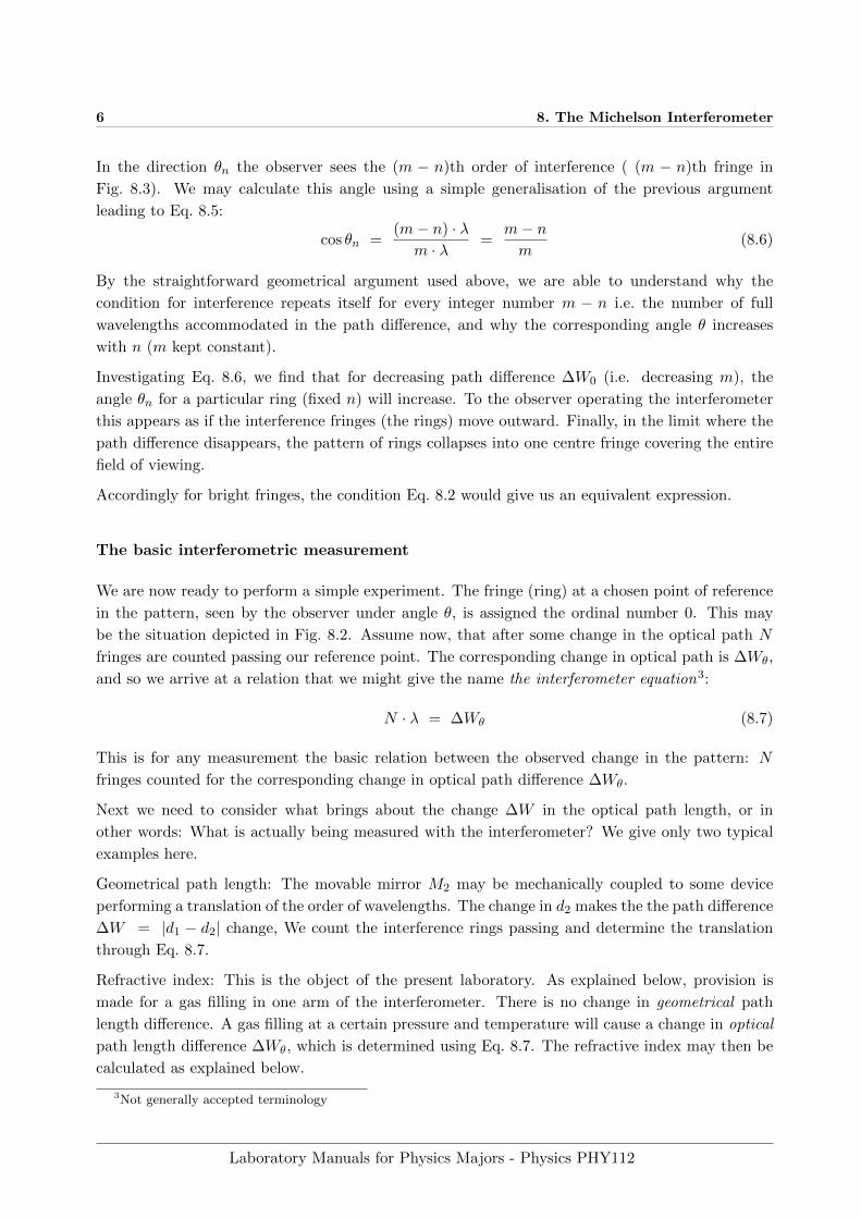
The interference conditions leading to the the pattern in Fig. 8.3, may be qualitatively understood

as follows: On the optical axis interference results in a bright fringe (a centre spot) if the path

difference W0 corresponds to an integer number of wavelengths, m, the additional λ/2 from the

beam splitter being taken into account. The integer m is called the order of interference. In some

direction θ from the optical axis, where the path difference is W0 minus one full wavelength, i.e.

a total of m − 1, the condition is (the path length difference and the diffraction order (m − n)

decreases with increasing angle θ):

∆Wθ = (m− 1) · λ (8.3)

The corresponding angle θ is the direction from the observer where the first bright fringe (a ring)

outside the central spot is seen, and we may calculate it as follows. From the triangle in Fig. 8.2

we immediately find that:

∆Wθ = ∆W0 · cos θ (8.4)

Using Eq. 8.1 and Eq. 8.3 for we obtain:

cos θ =(m− 1) · λm · λ

=m− 1

m(8.5)



In the direction θn the observer sees the (m − n)th order of interference ( (m − n)th fringe in

Fig. 8.3). We may calculate this angle using a simple generalisation of the previous argument

leading to Eq. 8.5:

cos θn =(m− n) · λm · λ

=m− nm

(8.6)

By the straightforward geometrical argument used above, we are able to understand why the

condition for interference repeats itself for every integer number m − n i.e. the number of full

wavelengths accommodated in the path difference, and why the corresponding angle θ increases

with n (m kept constant).

Investigating Eq. 8.6, we find that for decreasing path difference ∆W0 (i.e. decreasing m), the

angle θn for a particular ring (fixed n) will increase. To the observer operating the interferometer

this appears as if the interference fringes (the rings) move outward. Finally, in the limit where the

path difference disappears, the pattern of rings collapses into one centre fringe covering the entire

field of viewing.

Accordingly for bright fringes, the condition Eq. 8.2 would give us an equivalent expression.

The basic interferometric measurement

We are now ready to perform a simple experiment. The fringe (ring) at a chosen point of reference

in the pattern, seen by the observer under angle θ, is assigned the ordinal number 0. This may

be the situation depicted in Fig. 8.2. Assume now, that after some change in the optical path N

fringes are counted passing our reference point. The corresponding change in optical path is ∆Wθ,

and so we arrive at a relation that we might give the name the interferometer equation3:

N · λ = ∆Wθ (8.7)

This is for any measurement the basic relation between the observed change in the pattern: N

fringes counted for the corresponding change in optical path difference ∆Wθ.

Next we need to consider what brings about the change ∆W in the optical path length, or in

other words: What is actually being measured with the interferometer? We give only two typical

examples here.

Geometrical path length: The movable mirror M2 may be mechanically coupled to some device

performing a translation of the order of wavelengths. The change in d2 makes the the path difference

∆W = |d1 − d2| change, We count the interference rings passing and determine the translation

through Eq. 8.7.

Refractive index: This is the object of the present laboratory. As explained below, provision is

made for a gas filling in one arm of the interferometer. There is no change in geometrical path

length difference. A gas filling at a certain pressure and temperature will cause a change in optical

path length difference ∆Wθ, which is determined using Eq. 8.7. The refractive index may then be

calculated as explained below.

3Not generally accepted terminology


8.2. THEORY 7

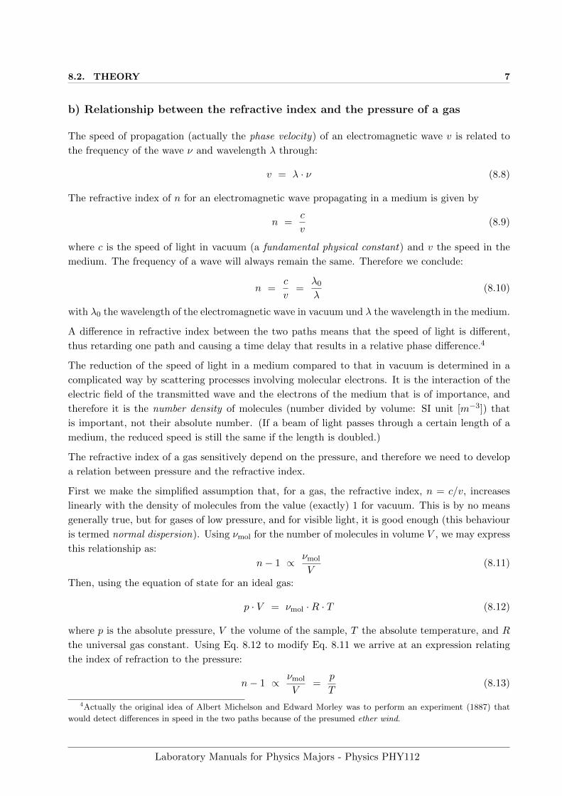
b) Relationship between the refractive index and the pressure of a gas

The speed of propagation (actually the phase velocity) of an electromagnetic wave v is related to

the frequency of the wave ν and wavelength λ through:

v = λ · ν (8.8)

The refractive index of n for an electromagnetic wave propagating in a medium is given by

n =c

v(8.9)

where c is the speed of light in vacuum (a fundamental physical constant) and v the speed in the

medium. The frequency of a wave will always remain the same. Therefore we conclude:

n =c

v=

λ0λ

(8.10)

with λ0 the wavelength of the electromagnetic wave in vacuum und λ the wavelength in the medium.

A difference in refractive index between the two paths means that the speed of light is different,

thus retarding one path and causing a time delay that results in a relative phase difference.4

The reduction of the speed of light in a medium compared to that in vacuum is determined in a

complicated way by scattering processes involving molecular electrons. It is the interaction of the

electric field of the transmitted wave and the electrons of the medium that is of importance, and

therefore it is the number density of molecules (number divided by volume: SI unit [m−3]) that

is important, not their absolute number. (If a beam of light passes through a certain length of a

medium, the reduced speed is still the same if the length is doubled.)

The refractive index of a gas sensitively depend on the pressure, and therefore we need to develop

a relation between pressure and the refractive index.

First we make the simplified assumption that, for a gas, the refractive index, n = c/v, increases

linearly with the density of molecules from the value (exactly) 1 for vacuum. This is by no means

generally true, but for gases of low pressure, and for visible light, it is good enough (this behaviour

is termed normal dispersion). Using νmol for the number of molecules in volume V , we may express

this relationship as:

n− 1 ∝ νmol

V(8.11)

Then, using the equation of state for an ideal gas:

p · V = νmol ·R · T (8.12)

where p is the absolute pressure, V the volume of the sample, T the absolute temperature, and R

the universal gas constant. Using Eq. 8.12 to modify Eq. 8.11 we arrive at an expression relating

the index of refraction to the pressure:

n− 1 ∝ νmol

V=

p

T(8.13)

4Actually the original idea of Albert Michelson and Edward Morley was to perform an experiment (1887) that

would detect differences in speed in the two paths because of the presumed ether wind.



which at constant temperature T may be written:

n− 1 = a · pT

or n = 1 +a

T· p (8.14)

where a is a factor of proportionality. Written in this way, a/T would appear as the slope in a

diagram of n plotted against the pressure p. Under the assumptions made, we have found a linear

relationship between the refractive index and the pressure, valid for constant temperature. The

constant of proportionality a will have to be determined to make the relation useful, and this is

the object of our experiment.

c) Measuring refractive indices by means of the Michelson interferometer

The principle of a measurement with the interferometer was established above in Eq. 8.7; it describes

what our equipment is able to accomplish. The relationship we would like investigate, our theory,

is laid down in Eq. 8.14, where the constant a is unknown. Therefore we need to device a method

of analysis that connects experiment with theory such that the constant a can be determined. In

essence, this is what experimental physicists is commonly confronted with.

In the present experiment, one path of the interferometer remains unchanged for reference, but the

other is modified such that it can receive a filling of gas at different pressures. For this purpose

a cylindrical cell of precisely known length L is installed, here in the path containing mirror S2.

The cell has glass windows at both ends, and it is necessary to compensate for the optical path the

beam travels through these in order to relate unambiguously a change in the observed pattern to

a change in refractive index. This is done by putting two identical windows also in the reference

path.

The geometrical path length L of the cell is kept constant. Since the optical path through the gas

cell is n · L, any observed change in the pattern is therefore related to a change of the refractive

index n of the gas in the cell (given that the compensations mentioned above have been properly

made).

In order to show that the two paths do not have to be equal, we assume that there is an initial

geometrical difference d that remains unchanged throughout the experiment. For the path difference

at the lowest pressure attained, pmin, at which the corresponding refractive index is nmin, we write:

∆Wmin = d+ 2L · nmin (8.15)

and for some arbitrary pressure p:

∆W = d+ 2L · n (8.16)

As we change the pressure from pmin, to the arbitrary pressure p, whilst keeping the temperature

constant at Texp, the corresponding change in optical path length difference will be:

∆W −∆Wmin = ((d+ 2L · n)− (d+ 2L · nmin)) = 2L · (n− nmin) (8.17)

Thus an initial geometrical path difference d, which we prefer to have for reasons explained else-

where, does not matter. Again the factor of 2 on the right enters because both paths are traversed


8.2. THEORY 9

twice. In Eq. 8.7 we may remove index θ since it is valid for any directions from the observer. As

the pressure changes from pmin to p, the number of fringes N travelling across the point of reference

in the pattern is, using Eqs. 8.7 and 8.17:

N =1

λ· (∆W −∆Wmin) =

2L

λ· (n− nmin) (8.18)

which we rewrite with a simple algebraic manipulation as:

N =2L

λ((n− 1)− (nmin − 1)) (8.19)

allowing us to utilise the result in Eq. 8.14:

N =2L

λ(a

Tp− a

Tpmin) =

2L

λ

a

T(p− pmin) (8.20)

Finally we arrive at the relation:Nλ

2L=

a

Texp·∆p (8.21)

where we defined ∆p ≡ p− pmin for convenience, and explicitly write T ≡ Texp for clarity. We have

here arrived at a linear relation for the two measurable variables, the accumulated number of fringes

N and the corresponding pressure difference ∆p. This is the general interferometer equation 8.7

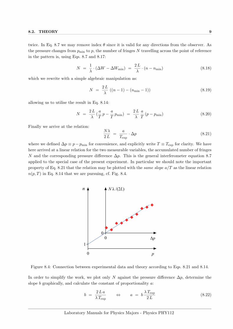
applied to the special case of the present experiment. In particular we should note the important

property of Eq. 8.21 that the relation may be plotted with the same slope a/T as the linear relation

n(p, T ) in Eq. 8.14 that we are pursuing, cf. Fig. 8.4.

Figure 8.4: Connection between experimental data and theory according to Eqs. 8.21 and 8.14.

In order to simplify the work, we plot only N against the pressure difference ∆p, determine the

slope b graphically, and calculate the constant of proportionality a:

b =2La

λTexp⇔ a = b

λ Texp2L

(8.22)



We have now at hand a complete description of how n(p, Texp) depends on the absolute pressure

at constant temperature Texp as formulated by Eq. 8.14.

Note, that the factor of proportionality a cannot be calculated from Eq. 8.21, since the graph pro-

duced from the experimental data does not necessarily go through the origin because of unavoidable

measurement errors. The slope must be determined graphically as explained below.

Next we acknowledge that the refractive index n is a function of both temperature and pressure,

and write in full n(p, T ) or n(p, Texp) for a constant temperature Texp.

With the constant of proportionality a experimentally determined, we may write for the pressure

dependence of the refractive index (cf. Eq. 8.14):

n(p, Texp)− 1 =a

Texp· p (8.23)

For comparison with tabulated data, this result may be normalised to the refractive index n(p0, T0)

at standard conditions p0 and T0 (in IUPAC and ISO 2787 p0=100 kPa and T0=273.15 K are

chosen) using Eq. 8.14 and defining n(p0, T0) ≡ n0:

n0 = 1 +a · p0T0

(8.24)

In summary, the refractive index of a gas may be calculated at standard conditions for temperature

and pressure, if the change in the interference pattern as function of pressure is measured. The

wavelength λ of the source, the length L of the gas cell and the constant absolute temperature of

the gas Texp are assumed to be known.


8.3. EXPERIMENTAL 11

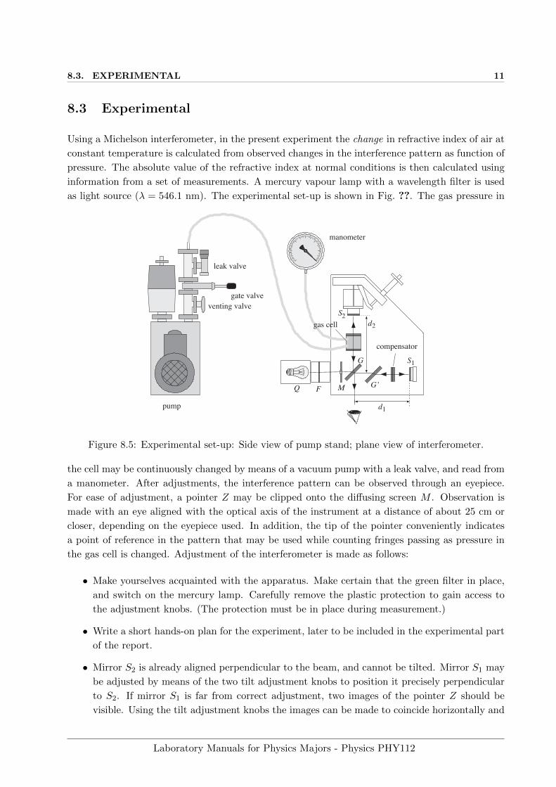
8.3 Experimental

Using a Michelson interferometer, in the present experiment the change in refractive index of air at

constant temperature is calculated from observed changes in the interference pattern as function of

pressure. The absolute value of the refractive index at normal conditions is then calculated using

information from a set of measurements. A mercury vapour lamp with a wavelength filter is used

as light source (λ = 546.1 nm). The experimental set-up is shown in Fig. ??. The gas pressure in

M

S1

S2

G’

G

leak valve

gate valveventing valve

pump

FQ

compensator

d1

d2

manometer

gas cell

Figure 8.5: Experimental set-up: Side view of pump stand; plane view of interferometer.

the cell may be continuously changed by means of a vacuum pump with a leak valve, and read from

a manometer. After adjustments, the interference pattern can be observed through an eyepiece.

For ease of adjustment, a pointer Z may be clipped onto the diffusing screen M . Observation is

made with an eye aligned with the optical axis of the instrument at a distance of about 25 cm or

closer, depending on the eyepiece used. In addition, the tip of the pointer conveniently indicates

a point of reference in the pattern that may be used while counting fringes passing as pressure in

the gas cell is changed. Adjustment of the interferometer is made as follows:

• Make yourselves acquainted with the apparatus. Make certain that the green filter in place,

and switch on the mercury lamp. Carefully remove the plastic protection to gain access to

the adjustment knobs. (The protection must be in place during measurement.)

• Write a short hands-on plan for the experiment, later to be included in the experimental part

of the report.

• Mirror S2 is already aligned perpendicular to the beam, and cannot be tilted. Mirror S1 may

be adjusted by means of the two tilt adjustment knobs to position it precisely perpendicular

to S2. If mirror S1 is far from correct adjustment, two images of the pointer Z should be

visible. Using the tilt adjustment knobs the images can be made to coincide horizontally and



vertically. In this position interference fringes should appear. If the adjustment of S1 is still

slightly wrong, almost straight fringes will appear. Turn the tilt adjustment knobs until the

centre of the pattern appears in the middle of the viewing field.

• A set of approximately concentric dark and bright ring-shaped interference fringes should

now be visible. Use the micrometer on the carrier holding mirror S2 to change its position.

Describe qualitatively how the pattern changes with the distance d2 Finally choose a setting

where the interference fringes are easily distinguished at the tip of Z. Carefully reposition

the plastic protection on the instrument.

• Read the temperature T at intervals during the experiment.

• Prepare a table containing columns for the number of fringes counted, accumulated number

of fringes N , gauge pressure, absolute pressure p, pressure difference ∆p.

• Evacuate the gas cell using the vacuum pump. Then switch off the pump, slowly open the

leak valve and observe the interference pattern change as the pressure is increasing. The

fringe at the starting pressure (lowest attainable) is given the ordinal number 0. Count the

number of fringes as they travel across the tip of the pointer Z and read the pressure p at the

manometer for every tenth fringe that pass. Note that gauge pressure is indicated (relative

to atmospheric pressure), which has to be recalculated to absolute pressure.

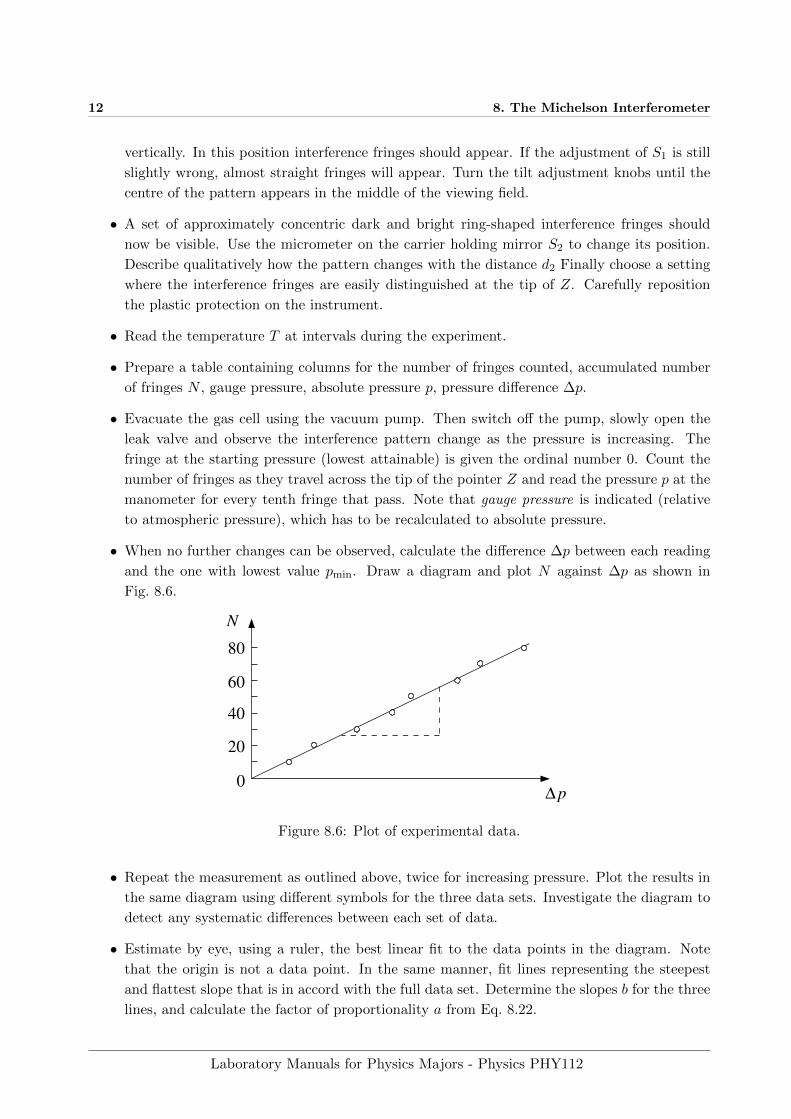
• When no further changes can be observed, calculate the difference ∆p between each reading

and the one with lowest value pmin. Draw a diagram and plot N against ∆p as shown in

Fig. 8.6.

0

20

40

60

80

N

p ∆

Figure 8.6: Plot of experimental data.

• Repeat the measurement as outlined above, twice for increasing pressure. Plot the results in

the same diagram using different symbols for the three data sets. Investigate the diagram to

detect any systematic differences between each set of data.

• Estimate by eye, using a ruler, the best linear fit to the data points in the diagram. Note

that the origin is not a data point. In the same manner, fit lines representing the steepest

and flattest slope that is in accord with the full data set. Determine the slopes b for the three

lines, and calculate the factor of proportionality a from Eq. 8.22.


8.3. EXPERIMENTAL 13

• Calculate the refractive index of air at standard conditions according to Eq. 8.24. Estimate

the measurement error from the spread in the slopes of the lines in the diagram. Values for

λ and L may be found at the lab bench.


M 8. The Michelson Interferometer - UZH -...

Documents

Transcript of M 8. The Michelson Interferometer - UZH -...