LUIZ GUSTAVO HAFEMANN - luizgh.github.io · maioria das bases, ... usando Redes Neurais...

LUIZ GUSTAVO HAFEMANN

AN ANALYSIS OF DEEP NEURAL NETWORKS FORTEXTURE CLASSIFICATION

Dissertation presented as partial requisite toobtain the Master’s degree. M.Sc. pro-gram in Informatics, Universidade Federal doParana.Advisor: Prof. Dr. Luiz Eduardo S. deOliveiraCo-Advisor: Dr. Paulo Rodrigo Cavalin

CURITIBA

2014

i

ACKNOWLEDGMENTS

I would like to thank my wife, Renata, for all the love, patience and understanding during

the last two years. I also want to thank my parents, for all the support during this time,

and during all my life. I would like to thank my research advisor, Dr. Luiz Oliveira,

and my co-advisor Dr. Paulo Cavalin, for all the guidance and assistance during this

time. Last but not least, I would like to thank Dennis Furlaneto for all the reviews of

my dissertation, and for the regular discussions in the coffee area, from where many ideas

emerged.

ii

CONTENTS

LIST OF FIGURES vi

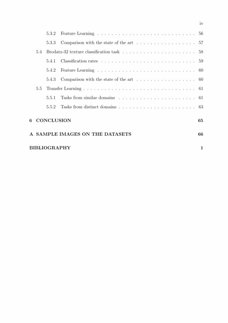
LIST OF TABLES vii

RESUMO viii

ABSTRACT x

1 INTRODUCTION 1

1.1 Motivation . . . . . . . . . . . . . . . . . . . . . . . . . . . . . . . . . . . . 2

1.2 Challenges . . . . . . . . . . . . . . . . . . . . . . . . . . . . . . . . . . . . 3

1.3 Objectives . . . . . . . . . . . . . . . . . . . . . . . . . . . . . . . . . . . . 3

1.4 Contributions . . . . . . . . . . . . . . . . . . . . . . . . . . . . . . . . . . 4

2 THEORETICAL BACKGROUND 6

2.1 Artificial Neural Networks . . . . . . . . . . . . . . . . . . . . . . . . . . . 6

2.1.1 Artificial Neuron . . . . . . . . . . . . . . . . . . . . . . . . . . . . 6

2.1.2 Multi-layer Neural Networks . . . . . . . . . . . . . . . . . . . . . . 7

2.1.2.1 Forward Propagation . . . . . . . . . . . . . . . . . . . . . 8

2.1.2.2 Training Objective . . . . . . . . . . . . . . . . . . . . . . 9

2.1.2.3 Backpropagation . . . . . . . . . . . . . . . . . . . . . . . 10

2.1.2.4 Training algorithm . . . . . . . . . . . . . . . . . . . . . . 11

2.2 Training Deep Neural Networks . . . . . . . . . . . . . . . . . . . . . . . . 13

2.3 Convolutional Neural Networks . . . . . . . . . . . . . . . . . . . . . . . . 14

2.3.1 Convolutional layers . . . . . . . . . . . . . . . . . . . . . . . . . . 15

2.3.2 Pooling layers . . . . . . . . . . . . . . . . . . . . . . . . . . . . . . 17

2.3.3 Locally-connected layers . . . . . . . . . . . . . . . . . . . . . . . . 18

2.4 Combining Classifiers . . . . . . . . . . . . . . . . . . . . . . . . . . . . . . 18

iii

2.5 Transfer Learning . . . . . . . . . . . . . . . . . . . . . . . . . . . . . . . . 19

2.5.1 Transfer Learning in Convolutional Neural Networks . . . . . . . . 20

3 STATE-OF-THE-ART 22

3.1 Deep learning review on the CIFAR-10 dataset . . . . . . . . . . . . . . . . 22

3.1.1 Summary of the CIFAR-10 top results . . . . . . . . . . . . . . . . 24

4 METHODOLOGY 27

4.1 Texture datasets . . . . . . . . . . . . . . . . . . . . . . . . . . . . . . . . 28

4.1.1 Forest Species datasets . . . . . . . . . . . . . . . . . . . . . . . . . 28

4.1.2 Writer identification . . . . . . . . . . . . . . . . . . . . . . . . . . 29

4.1.3 Music genre classification . . . . . . . . . . . . . . . . . . . . . . . . 29

4.1.4 Brodatz texture classification . . . . . . . . . . . . . . . . . . . . . 30

4.1.5 Summary of the datasets . . . . . . . . . . . . . . . . . . . . . . . . 31

4.2 Training Method for CNNs on Texture Datasets . . . . . . . . . . . . . . . 31

4.2.1 Image resize and patch extraction . . . . . . . . . . . . . . . . . . . 32

4.2.2 CNN architecture and training . . . . . . . . . . . . . . . . . . . . . 33

4.2.3 Combining Patches for testing . . . . . . . . . . . . . . . . . . . . . 35

4.3 Training Method for Transfer Learning . . . . . . . . . . . . . . . . . . . . 37

5 EXPERIMENTAL RESULTS 42

5.1 Forest species recognition tasks . . . . . . . . . . . . . . . . . . . . . . . . 42

5.1.1 Classification rates . . . . . . . . . . . . . . . . . . . . . . . . . . . 43

5.1.2 Feature Learning . . . . . . . . . . . . . . . . . . . . . . . . . . . . 46

5.1.3 Comparison with the state of the art . . . . . . . . . . . . . . . . . 47

5.2 Author Identification tasks . . . . . . . . . . . . . . . . . . . . . . . . . . . 49




5.3 Music Genre classification task . . . . . . . . . . . . . . . . . . . . . . . . . 54


iv



5.4 Brodatz-32 texture classification task . . . . . . . . . . . . . . . . . . . . . 58




5.5 Transfer Learning . . . . . . . . . . . . . . . . . . . . . . . . . . . . . . . . 61

5.5.1 Tasks from similar domains . . . . . . . . . . . . . . . . . . . . . . 61

5.5.2 Tasks from distinct domains . . . . . . . . . . . . . . . . . . . . . . 63

6 CONCLUSION 65

A SAMPLE IMAGES ON THE DATASETS 66

BIBLIOGRAPHY 1

v

LIST OF FIGURES

2.1 A single artificial neuron. . . . . . . . . . . . . . . . . . . . . . . . . . . . . 7

2.2 A neural network composed of three layers. . . . . . . . . . . . . . . . . . . 8

2.3 Architecture of a convolution network for traffic sign recognition [36]. . . . 14

2.4 Sample feature maps learned by a convolution network for traffic sign recog-

nition [36] . . . . . . . . . . . . . . . . . . . . . . . . . . . . . . . . . . . . 15

2.5 The forward propagation phase of a convolutional layer. . . . . . . . . . . . 16

2.6 The forward propagation phase of a pooling layer. . . . . . . . . . . . . . . 17

2.7 Transfer learning from the ImagetNet dataset to the Pascal VOC dataset . 21

4.1 An overview of the Pattern Recognition process. . . . . . . . . . . . . . . . 27

4.2 The zoning methodology used by Costa [56]. . . . . . . . . . . . . . . . . . 30

4.3 The Deep Convolutional Neural Network architecture. . . . . . . . . . . . . 33

4.4 The training procedure using random patches . . . . . . . . . . . . . . . . 36

4.5 The testing procedure using non-overlapping patches . . . . . . . . . . . . 38

4.6 The training procedure for transfer learning . . . . . . . . . . . . . . . . . 40

4.7 The testing procedure for transfer learning . . . . . . . . . . . . . . . . . . 41

5.1 Error rates on the Forest Species dataset with Macroscopic images, for

CNNs trained with different hyperparameters. . . . . . . . . . . . . . . . . 43

5.2 Error rates on the Forest Species dataset with Microscopic images, for

CNNs trained with different hyperparameters. . . . . . . . . . . . . . . . . 44

5.3 Random predictions for patches on the Testing set (Macroscopic images) . 45

5.4 Random predictions for patches on the Testing set (Microscopic images) . . 46

5.5 Filters learned by the first convolutional layers of models trained on the

Macroscopic images dataset. . . . . . . . . . . . . . . . . . . . . . . . . . . 47

5.6 Filters learned by the first convolutional layer of a model trained on the

Microscopic images dataset. . . . . . . . . . . . . . . . . . . . . . . . . . . 47

vi

5.7 Error rates on the IAM dataset, for CNNs trained with different hyperpa-

rameters. . . . . . . . . . . . . . . . . . . . . . . . . . . . . . . . . . . . . . 50

5.8 Error rates on the BFL dataset, for CNNs trained with different hyperpa-

rameters. . . . . . . . . . . . . . . . . . . . . . . . . . . . . . . . . . . . . . 51

5.9 Random predictions for patches on the IAM Testing set . . . . . . . . . . . 52

5.10 Random predictions for patches on the BFL Testing set . . . . . . . . . . . 52


IAM dataset. . . . . . . . . . . . . . . . . . . . . . . . . . . . . . . . . . . 53


BFL dataset. . . . . . . . . . . . . . . . . . . . . . . . . . . . . . . . . . . 53

5.13 Error rates on the Latin Music Dataset, for CNNs trained with different

hyperparameters. . . . . . . . . . . . . . . . . . . . . . . . . . . . . . . . . 55

5.14 Random predictions for test patches on the Latin Music Dataset . . . . . . 56


Latin Music dataset. . . . . . . . . . . . . . . . . . . . . . . . . . . . . . . 56

5.16 Error rates on the Brodatz dataset, for CNNs trained with different hyper-

parameters. . . . . . . . . . . . . . . . . . . . . . . . . . . . . . . . . . . . 59

5.17 Random predictions for patches on the Brodatz-32 Testing set . . . . . . . 60


Brodatz-32 dataset. . . . . . . . . . . . . . . . . . . . . . . . . . . . . . . . 60

A.1 Sample images from the macroscopic Brazilian forest species dataset . . . . 66

A.2 Sample images from the microscopic Brazilian forest species dataset . . . . 67

A.3 Sample texture created from the Latin Music Dataset dataset. . . . . . . . 67

A.4 Sample image from the BFL dataset, and the associated texture. [53] . . . 68

A.5 Sample image from the IAM dataset, and the associated texture. [8] . . . . 68

A.6 Sample images from the Brodatz-32 dataset [58] . . . . . . . . . . . . . . . 69

vii

LIST OF TABLES

3.1 Comparison of top published results on the CIFAR-10 dataset . . . . . . . 26

4.1 Summary of the properties of the datasets . . . . . . . . . . . . . . . . . . 31

5.1 Classification on the Macroscopic images dataset . . . . . . . . . . . . . . . 48

5.2 Classification on the Microscopic images dataset . . . . . . . . . . . . . . . 48

5.3 Classification on the IAM dataset . . . . . . . . . . . . . . . . . . . . . . . 53

5.4 Classification on the BFL dataset . . . . . . . . . . . . . . . . . . . . . . . 54

5.5 Classification on the Latin Music dataset . . . . . . . . . . . . . . . . . . . 57

5.6 Confusion Matrix on the Latin Music Dataset classification (%) - Our method 58

5.7 Confusion Matrix on the Latin Music Dataset classification (%) - Costa et

al.[9] . . . . . . . . . . . . . . . . . . . . . . . . . . . . . . . . . . . . . . . 58

5.8 Classification on the Brodatz-32 dataset . . . . . . . . . . . . . . . . . . . 61

5.9 Classification on the Macroscopic Forest species dataset . . . . . . . . . . . 62



5.12 Classification on the Brodatz-32 dataset . . . . . . . . . . . . . . . . . . . 64

viii

RESUMO

Classificacao de texturas e um problema na area de Reconhecimento de Padroes com uma

ampla gama de aplicacoes. Esse problema e geralmente tratado com o uso de descritores

de texturas e modelos de reconhecimento de padroes, tais como Maquinas de Vetores de

Suporte (SVM) e Regra dos K vizinhos mais proximos (KNN).

O metodo classico para enderecar o problema depende do conhecimento de especialis-

tas no domınio para a criacao de extratores de caracterısticas relevantes (discriminantes),

criando-se varios descritores de textura, cada um voltado para diferentes cenarios (por

exemplo, descritores de textura que sao invariantes a rotacao, ou invariantes ao borra-

mento da imagem). Uma estrategia diferente para o problema e utilizar algoritmos para

aprender os descritores de textura, ao inves de construı-los manualmente. Esse e um dos

objetivos centrais de modelos de Arquitetura Profunda – modelos compostos por multiplas

camadas, que tem recebido grande atencao nos ultimos anos. Um desses metodos, cha-

mado de Rede Neural Convolucional, tem sido utilizado para atingir o estado da arte em

varios problemas de visao computacional como, por exemplo, no problema de reconheci-

mento de objetos. Entretanto, esses metodos ainda nao sao amplamente explorados para

o problema de classificacao de texturas.

A presente dissertacao preenche essa lacuna, propondo um metodo para treinar Redes

Neurais Convolucionais para problemas de classificacao de textura, lidando com os desafios

e tomando em consideracao as caracterısticas particulares desse tipo de problema. O

metodo proposto foi testado em seis bases de dados de texturas, cada uma apresentando

um desafio diferente, e resultados proximos ao estado da arte foram observados para a

maioria das bases, obtendo-se resultados superiores em duas das seis bases de dados.

Por fim, e apresentado um metodo para transferencia de conhecimento entre diferen-

tes problemas de classificacao de texturas, usando Redes Neurais Convolucionais. Os

experimentos conduzidos demonstraram que essa tecnica pode melhorar o desempenho

dos classificadores em problemas de textura com bases de dados pequenas, utilizando o

ix

conhecimento aprendido em um problema similar, que possua uma grande base de dados.

Palavras chave: Reconhecimento de padroes; Classificacao de Texturas; Redes Neu-

rais Convolucionais

x

ABSTRACT

Texture classification is a Pattern Recognition problem with a wide range of applications.

This task is commonly addressed using texture descriptors designed by domain experts,

and standard pattern recognition models, such as Support Vector Machines (SVM) and

K-Nearest Neighbors (KNN).

The classical method to address the problem relies on expert knowledge to build rel-

evant (discriminative) feature extractors. Experts are required to create multiple texture

descriptors targeting different scenarios (e.g. features that are invariant to image rota-

tion, or invariant to blur). A different approach for this problem is to learn the feature

extractors instead of using human knowledge to build them. This is a core idea behind

Deep Learning, a set of models composed by multiple layers that are receiving increased

attention in recent years. One of these methods, Convolutional Neural Networks, has been

used to set the state-of-the-art in many computer vision tasks, such as object recognition,

but are not yet widely explored for the task of texture classification.

The present work address this gap, by proposing a method to train Convolutional

Neural Networks for texture classification tasks, facing the challenges of texture recogni-

tion and taking advantage of particular characteristics of textures. We tested our method

on six texture datasets, each one posing different challenges, and achieved results close to

the state-of-the-art in the majority of the datasets, surpassing the best previous results

in two of the six tasks.

We also present a method to transfer learning across different texture classification

problems using Convolutional Neural Networks. Our experiments demonstrated that

this technique can improve the performance on tasks with small datasets, by leveraging

knowledge learned from tasks with larger datasets.

Keywords: Pattern Recognition; Texture Classification; Convolutional Neural Net-

works

1

CHAPTER 1

INTRODUCTION

Texture classification is an important task in image processing and computer vision, with

a wide range of applications, such as computer-aided medical diagnosis [1], [2], [3], clas-

sification of forest species [4], [5], [6], classification in aerial/satellite images [7], writer

identification and verification [8] and music genre classification [9].

Texture classification commonly follows the standard procedure for pattern recogni-

tion, as described by Bishop et al. in [10]: extract relevant features, train a model using

a training dataset, and evaluate the model on a held-out test set.

Many methods have been proposed for the feature extraction phase on texture clas-

sification problems, as reviewed by Zhang et al. [11] and tested on multiple datasets by

Guo et al. [12]. Noteworthy techniques are: Gray-Level Co-occurrence Matrices (GLCM),

the Local Binary Pattern operator (LBP), Local Phase Quantization (LPQ), and Gabor

filters.

The methods above rely on domain experts to build the feature extractors to be used

for classification. An alternative approach is to use models that learn directly from raw

data, for instance, directly from pixels in the case of images. The intuition is using such

methods to learn multiple intermediate representations of the input, in layers, in order to

better represent a given problem. Consider an example for object recognition in an image:

the inputs for the model can be the raw pixels in the image. Each layer of the model

constitutes an equivalent of feature detectors, transforming the data into more abstract

(and hopefully useful) representations. The initial layers can learn low-level features,

such as detecting edges, and subsequent layers learn higher-level representations, such as

detecting more complex local shapes, up to high-level representations, such as recognizing

a particular object [13]. In summary, the term Deep Learning refers to machine learning

models that have multiple layers, and techniques for effectively training these models,

2

commonly building Deep Neural Networks or Deep Belief Networks [14], [15].

Methods using deep architectures have set the state-of-the-art in many domains in

recent years, as reviewed by Bengio in [13] and [16]. Besides improving the accuracy on

different pattern recognition problems, one of the fundamental goals of Deep Learning is

to move machine learning towards the automatic discovery of multiple levels of represen-

tation, reducing the need for feature extractors developed by domain experts [16]. This is

especially important, as noted by Bengio in [13], for domains where the features are hard

to formalize, such as for object recognition and speech recognition tasks.

In the task of object recognition, deep architectures have been widely used to achieve

state-of-the-art results, such as in the CIFAR dataset[17] where the top published re-

sults use Convolutional Neural Networks (CNN) [18]. The tasks of object and texture

classification present similarities, such as the strong correlation of pixel intensities in the

2-D space, and present some differences, such as the ability to perform the classification

using only a relatively small fragment of a texture. In spite of the similarities with object

classification we observe that deep learning techniques are not yet widely used for tex-

ture classification tasks. Kivinen and Williams [19] used Restricted Boltzmann Machines

(RBMs) for texture synthesis, and Luo et al. [20] used spike-and-slab RBMs for texture

synthesis and inpainting. Both consider using image pixels as input, but they do not

consider training deep models for classification among several classes. Titive et al. [21]

used convolutional neural networks on the Brodatz texture dataset, but considered only

low resolution images, and a small number of classes.

The similarities between texture classification and object recognition, and the good

results demonstrated by using deep architectures for object recognition suggest that these

techniques could be successfully applied for texture classification.

1.1 Motivation

There is a considerable set of potential applications for texture recognition, as briefly

presented above. However, despite the reported success of classical texture classification

techniques in many of these tasks, these problems are still not resolved and are subject

3

of active research, with potential to increase recognition rates.

A second motivation is that traditional machine learning techniques often require

human expertise and knowledge to hand-engineer features, for each particular domain,

to be used in classification and regression tasks. It can be considered that the actual

intelligence in such systems is therefore in the creation of such features, instead of the

machine learning algorithm that uses them. Therefore, using techniques that do not

rely on expert-defined feature extractors can make it easier to develop effective machine

learning models for novel datasets, without requiring the test and selection of a large set

of possible feature extractors.

1.2 Challenges

Here is a set of challenges in applying deep learning techniques to texture classification

problems:

• Image size: The majority of the image-related tasks where deep learning was success-

fully applied used images of small size. Examples: MNIST (28x28 pixels), STL-10

(96x96), Norb (108x108), Cifar-10 and Cifar-100 (32x32).

• Model size and Training time: One exception to dataset list above is the ImageNet

dataset, which consists in high-resolution images of variable sizes. The best results

on this dataset, however, require significant usage of computer resources (such as 16

thousands cores running for three days [22]). The texture datasets commonly consist

of higher resolution images, and therefore different techniques need to be tested, in

order to classify the textures without using too much computing resources.

1.3 Objectives

The main objective of this research is to test whether or not deep learning models, in

particular Convolutional Neural Networks, can be successfully applied for texture classi-

fication problems.

4

More specifically, we test these methods on multiple texture datasets, developing a

method to cope with the high-resolution texture images without requiring models that

are too large, or that require too much computing power to train. Six texture datasets

were selected for testing, representing different domain problems, and containing different

characteristics, such as image sizes, number of classes and number of samples per class.

As part of this effort, we assess if it is possible to obtain a generic framework that brings

good results for multiple texture problems.

After training the models on each dataset, the accuracy of the deep models are com-

pared with the state-of-the-art results achieved using the classical texture descriptors.

Finally, another objective of this research is to evaluate a method of Transfer Learning

for texture classification. Transfer Learning consists in using a model trained in one task

to improve results on another task. This is particularly interesting when using Deep

Neural Networks, as these models often require large datasets to be effectively trained.

We investigate the hypothesis that we can leverage a neural network trained on a large

dataset to improve the results on other tasks, including tasks with smaller datasets.

1.4 Contributions

In this dissertation, we propose a method to train Convolutional Neural Networks on

texture classification datasets. We explore the hypothesis that, for most textures, we

can classify a texture using only a small fragment of the image. This allowed us to use

datasets with large images and still keep the neural network models with a reasonable

size. It also enabled us to use a strategy of classifying parts of the images individually,

and subsequently combine the results of multiple predictions of the same texture image,

achieving good results. We validated our method using six texture datasets, each one

posing different challenges. The proposed method obtained excellent results for some types

of tasks (in particular, tasks with large datasets), achieving state-of-the-art performance.

We also propose a method to transfer learning across texture classification tasks, using

a Convolutional Neural Network. We explore the idea that the weights learned by a

Convolutional Neural Network can be used similarly to feature extractors, evaluating the

5

hypothesis that the features learned by the model in one dataset can be relevant for

other tasks. We explore this idea by using a CNN trained in one dataset to improve

the performance on a task with another dataset. We validated this proposal in four

experiments, considering both cases where the tasks are from similar domains, and cases

where the tasks are from different domains. We found that the method for transfer

learning was particularly useful to improve the performance on tasks with small datasets,

even when transfer knowledge to a task from a different domain.

The remainder of this dissertation is organized as follows. We present the theoretical

background of neural networks and transfer learning in Chapter 2. In Chapter 3 we review

the state-of-the-art of using deep neural networks for a similar task: object recognition.

In Chapter 4, we present our method for training CNNs for texture classification, and

the method to transfer learning across texture classification tasks. The experimental

evaluation is presented in Chapter 5, and we conclude our work in Chapter 6. Appendix

A lists samples from the texture datasets used in the experimental evaluation.

6

CHAPTER 2

THEORETICAL BACKGROUND

To make this document self-contained, this Chapter reviews the theoretical foundations

for Deep Neural Networks. The basic concepts of Artificial Neural Networks are presented,

starting with the original models that date back from 1943. The concept of Deep Neural

networks is then reviewed, with the recent advancements in the field that enabled training

Deep Neural Networks successfully. Afterwards, we review the theoretical foundations of

other procedures and methods used in the present work: the combination of multiple

classifiers, and transferring knowledge across different learning tasks.

2.1 Artificial Neural Networks

Artificial Neural Networks are mathematical models that use a collection of simple compu-

tational units, called Neurons, interlinked in a network. These models are used in a variety

of pattern recognition tasks, such as speech recognition, object recognition, identification

of cancerous cells, among others [23]

Artificial Neural Networks date back to 1943, with work by McCulloch and Pitts [24].

The motivation for studying neural networks was the fact that the human brain was

superior to a computer at many tasks, a statement that holds true even today for tasks

such as recognizing objects and faces, in spite of the huge advances in the processing

speed in modern computers.

2.1.1 Artificial Neuron

The neuron is the basic unit on Artificial Neural Networks, and it is used to construct

more powerful models. A typical set of equations to describe Neural Networks is provided

in [25], and is listed below for completeness. A single neuron implements a mathematical

function given its inputs, to provide an output, as described in equation 2.1 and illustrated

7

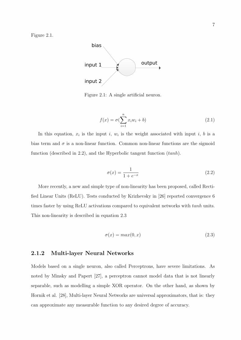
Figure 2.1.

input 1 output

bias

input 2

Figure 2.1: A single artificial neuron.

f(x) = σ(n

∑

i=1

xiwi + b) (2.1)

In this equation, xi is the input i, wi is the weight associated with input i, b is a

bias term and σ is a non-linear function. Common non-linear functions are the sigmoid

function (described in 2.2), and the Hyperbolic tangent function (tanh).

σ(x) =1

1 + e−x(2.2)

More recently, a new and simple type of non-linearity has been proposed, called Recti-

fied Linear Units (ReLU). Tests conducted by Krizhevsky in [26] reported convergence 6

times faster by using ReLU activations compared to equivalent networks with tanh units.

This non-linearity is described in equation 2.3

σ(x) = max(0, x) (2.3)

2.1.2 Multi-layer Neural Networks

Models based on a single neuron, also called Perceptrons, have severe limitations. As

noted by Minsky and Papert [27], a perceptron cannot model data that is not linearly

separable, such as modelling a simple XOR operator. On the other hand, as shown by

Hornik et al. [28], Multi-layer Neural Networks are universal approximators, that is: they

can approximate any measurable function to any desired degree of accuracy.

8

A Multi-layer Neural network consists of several layers of neurons. The first layer is

composed of the inputs to the neural network, it is followed by one or more hidden layers,

up to a last layer that contains the outputs of the network. In the simplest configuration,

each layer l is fully connected with the adjacent layers (l− 1 and l+ 1), and produces an

output vector yl given the output vector of the previous layer yl−1. The output of a layer

is calculated by applying the neuron activation function for all neurons on the layer, as

noted in equation 2.4, where W l is a matrix of weights assigned to each pair of neurons

from layer l and l − 1, and bl is a vector of bias terms for each neuron in layer l.

yl = σ(W lyl−1 + bl) (2.4)

Inputs OutputHidden layer(s)

Figure 2.2: A neural network composed of three layers.

2.1.2.1 Forward Propagation

The phase called forward propagation consists in applying the neuron activation equation

(2.1) starting from first hidden layer, up to the output layer. For classification tasks, the

output layer commonly uses another activation function, called Softmax. Softmax is

particularly useful for the last layer as the function generates a well-formed probability

distribution on the outputs. The softmax equation is defined below (2.5 and 2.6). In

9

these equations, zli is the output of the layer (for neuron i) before the application of the

non-linearity, yli is the output of the layer for the neuron i, W li is a vector of weights

connecting each neuron on layer l − 1 to the neuron i on layer l and bli is a bias term for

the neuron. The summation term considers all neurons j on the layer l.

zli = W li y

l−1 + bli (2.5)

yli =ez

li

∑

j ezlj

(2.6)

2.1.2.2 Training Objective

In order to train the model, an error function, also called loss function, is defined.

This function calculates the error of the model predictions with respect to a dataset. The

objective of the training is to minimize the sum (or, equivalently, minimize the mean) of

this error function applied to all examples in the dataset. Commonly used loss functions

are the Squared Error function (SE), described in equation 2.7, and the Cross-Entropy

error function (CE), described in equation 2.8 (both equations describe the error for a

single example in the dataset). As analyzed by Golik et al [29], it can be shown that

the true posterior probability is a global minimum for both functions, and therefore a

Neural Network can be trained by minimizing either. On the other hand, in practice

using Cross-Entropy error leads to faster convergence, and therefore this error function

became more popular in recent years.

E =1

2

∑

c

(ylc − tc)2 (2.7)

E = −∑

c

(tc log ylc)

2 (2.8)

In these equations, ylc is the output of unit c in the last layer in the model (l), and tc

is the identity function applied to the true label t (refer to equation 2.9):

10

tc =

1, if t = c

0, otherwise

(2.9)

2.1.2.3 Backpropagation

The error function can be minimized using Gradient-Based Learning. This strategy con-

sists in taking partial derivatives of the error function with respect to the model pa-

rameters, and using these derivatives to iteratively update the parameters [30]. Efficient

learning algorithms can be used for this purpose if these gradients (partial derivatives)

can be computed analytically.

The phase called backpropagation consists in calculating the derivatives of the error

function with respect to the model’s parameters (weights and biases), by propagating the

error from the output layers, back to the initial layers, one layer at a time. Since each

layer in the Neural Network consists of simple functions using only the values from the

previous layer, we can use the chain rule to easily determine the derivatives analytically.

For instance, to calculate the gradient respective to the weights in a layer we have the

equation below, as described in [31]:

δE

δwhj

=δE

δyi

δyi

δzh

δzh

δwhj

(2.10)

Where yi is the output of the neuron, zh is the output before applying the activation

function, and whj’s are the weights.

In order to use this strategy, we need to calculate:

1. The derivative of the error with respect to the neurons in the last layer δE

δyLi

2. The derivative of the outputs yi with respect to the outputs before the activation

function zi, that isδyliδzli

3. The derivative of zj with respect to the weights wij, that isδzlj

δwli,j

4. The derivative of zj with respect to the bias bj, that isδzlj

δblj

11

5. The derivative of zj with respect to its inputs, that isδzlj

δyl−1

i

We start with the top layer, calculating the derivative of the error (Cross-Entropy)

with respect to zi. In this equation, ti is defined as above (in equation 2.9):

δE

δzli= yli − ti (2.11)

For the derivatives with respect to the weights, we obtain the formula:

δzlj

δwlij

= yl−1i (2.12)

For the derivatives with respect to the biases, we obtain the formula:

δzlj

δbli= 1 (2.13)

For the derivatives with respect to the inputs, we obtain the formula:

δzlj

δyl−1i

= wlij (2.14)

The equations above are sufficient to compute the derivatives with respect to the

weights and biases of the last layer, and the derivative with respect to the outputs of the

layer l − 1. The other equation necessary is the derivative of the activation function of

the layers 1 until l − 1 (that don’t use softmax). The derivative for the sigmoid function

is described below:

δyliδzli

= yli(1− yli) (2.15)

2.1.2.4 Training algorithm

Training the network consists in minimizing the error function (by updating the weights

and biases), often using the Stochastic Gradient Descent algorithm (SGD), or quasi-

Newton methods, such as L-BFGS (Limited memory Broyden-Fletcher-Goldfarb-Shanno

12

algorithm).

The SGD algorithm, as defined in [32], is described below at a high-level. The inputs

are: W - the weights and biases of the network, (X, y) - the dataset, batch size - the

number of training examples that are used in each iteration, and α, the learning rate.

For notation simplicity, all the model parameters are represented in W . In practice, each

layer usually defines a 2-dimensional weight matrix and a 1-dimensional bias vector. In

summary, SGD iterates over mini-batches of the dataset, performing forward-propagation

followed by a back-propagation to calculate the error derivatives with respect to the

parameters. The weights are updated using these derivatives and a new mini-batch is

used. This procedure is repeated until a convergence criterion is reached. Common

convergence criteria are: a maximum number of epochs (number of times that the whole

training set was used); a desired value for the cost function is reached; or training until

the cost function shows no improvement in a number of iterations.

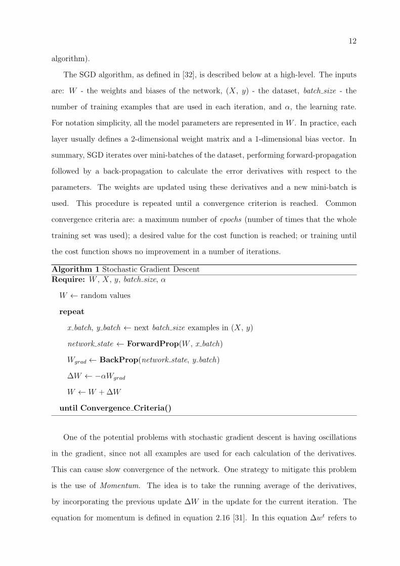
Algorithm 1 Stochastic Gradient Descent

Require: W , X, y, batch size, α

W ← random values

repeat

x batch, y batch ← next batch size examples in (X, y)

network state ← ForwardProp(W , x batch)

Wgrad ← BackProp(network state, y batch)

∆W ← −αWgrad

W ← W +∆W

until Convergence Criteria()

One of the potential problems with stochastic gradient descent is having oscillations

in the gradient, since not all examples are used for each calculation of the derivatives.

This can cause slow convergence of the network. One strategy to mitigate this problem

is the use of Momentum. The idea is to take the running average of the derivatives,

by incorporating the previous update ∆W in the update for the current iteration. The

equation for momentum is defined in equation 2.16 [31]. In this equation ∆wt refers to

13

the update to the weights in iteration t, and β is a factor for the momentum, usually

taken between 0.5 and 1.0 [31].

∆w(t)ij = −α

δE(t)

δwi

+ β∆w(t−1)ij (2.16)

2.2 Training Deep Neural Networks

The depth of an architecture refers to the number of non-linear operations that are com-

posed on the network. While many of the early successful applications of neural networks

used shallow architectures (up to 3 levels), the mammal brain is organized in a deep ar-

chitecture. The brain appears to process information through multiple stages, which is

particularly clear in the primate visual system[13]. Deep Neural Networks have been in-

vestigated for decades, but training deep networks consistently yielded poor results, until

very recently. It was observed in many experiments that deep networks are harder to train

than shallow networks, and that training deep networks often get stuck in apparent local

minima (or plateaus) when starting with random initialization of the network parameters.

It was discovered, however, that better results could be achieved by pre-training each layer

with an unsupervised learning algorithm [14]. In 2006, Hinton obtained good results using

Restricted Boltzmann Machines (a generative model) to perform unsupervised training

of the layers [14]. The goal of this training was to obtain a model that could capture

patterns in the data, similarly to a feature descriptor, not using the dataset labels. The

weights learned by this unsupervised training were then used to initialize neural networks.

Similar results were reported using auto-encoders for training each layer [15]. These ex-

periments identified that layers could be pre-trained one at a time, in a greedy layer-wise

format. After the layers are pre-trained, the learned weights are used to initialize the

neural network, and then the standard back-propagation algorithm is used for fine-tuning

the network. The advantage of unsupervised pre-training was demonstrated in several

statistical comparisons [15], [33], [34], until recently, when deep neural networks trained

only with supervised learning started to register similar results in some tasks (like object

recognition). Ciresan et al. [18] demonstrate that properly trained deep neural networks

14

(with only supervised learning) are able to achieve top results in many tasks, although

not denying that pre-training might help, especially in cases were little data is available

for training, or when there are massive amounts of unlabeled data.

On the task of image classification, the best published results use a particular type of

architecture called Convolutional Neural Network, which is described in the next section.

2.3 Convolutional Neural Networks

Convolutional networks combine three architectural ideas: local receptive fields, shared

(tied) weights and spatial or temporal sub-sampling [30]. This type of network was used

to obtain state-of-the-art results in the CIFAR-10 object recognition task [18] and, more

recently, to obtain state-of-the-art results in more challenging tasks such as the Ima-

geNet Large Scale Visual Recognition Challenge [35]. For both tasks, the training process

benefited from the significant speed-ups on processing using modern GPUs (Graphical

Processing Units), which are well suited for the implementation of convolutional net-

works.

The following sections describe the types of layers that compose a Convolutional Neural

Network. To illustrate the concept, Figure 2.3 shows a sample Convolutional Network.

Figure 2.3: Architecture of a convolution network for traffic sign recognition [36].

15

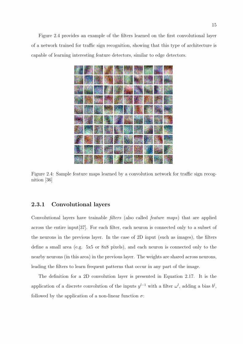
Figure 2.4 provides an example of the filters learned on the first convolutional layer

of a network trained for traffic sign recognition, showing that this type of architecture is

capable of learning interesting feature detectors, similar to edge detectors.

Figure 2.4: Sample feature maps learned by a convolution network for traffic sign recog-nition [36]

2.3.1 Convolutional layers

Convolutional layers have trainable filters (also called feature maps) that are applied

across the entire input[37]. For each filter, each neuron is connected only to a subset of

the neurons in the previous layer. In the case of 2D input (such as images), the filters

define a small area (e.g. 5x5 or 8x8 pixels), and each neuron is connected only to the

nearby neurons (in this area) in the previous layer. The weights are shared across neurons,

leading the filters to learn frequent patterns that occur in any part of the image.

The definition for a 2D convolution layer is presented in Equation 2.17. It is the

application of a discrete convolution of the inputs yl−1 with a filter ωl, adding a bias bl,

followed by the application of a non-linear function σ:

16

ylrc = σ(Fr∑

i=1

Fc∑

j=1

yl−1(r+i−1)(c+j−1)w

lij + bl) (2.17)

In this equation, ylrc is the output unit at {r, c}, Fr and Fc are the number of rows

and columns in the 2D filter, wlij is the value of the filter at position {i, j}, y

l−1(r+i−1)(c+j−1)

is the value of input to this layer, at position {r+ i− 1, c+ j− 1}, and bl is the bias term.

The forward propagation phase of a convolutional layer is illustrated in figure 2.5.

.*

X

.*

X

.*X

Input

Filter

output

Figure 2.5: The forward propagation phase of a convolutional layer.

The equation above is defined for all possible applications of the filter, that is, for

r ∈ {1, ..., Xr − Fr + 1} and c ∈ {1, ..., Xc − Fc + 1}, where Xr and Xc are the number of

rows and columns in the input to this layer. The convolutional layer can either apply the

filters for all possible inputs, or use a different strategy. Mainly to reduce computation

time, instead of applying the filter for all possible {r, c} pairs, only the pairs with distance

s are used, which is called the stride. A stride s = 1 is equivalent to apply the convolution

for all possible pairs, as defined above.

The inspiration for convolutional layers originated from models of the mammal visual

system. Modern research in the physiology of the visual system found it consistent with

the processing mechanism of convolutional neural networks, at least for quick recognition

of objects [13]. Although being a biological plausible model, the theoretical reasons for

the success of convolutional networks are not yet fully understood. One hypothesis is

17

that the small fan-in of the neurons (i.e. the number or input connections to the neurons)

helps the derivatives to propagate through many layers - instead of being diffused in a

large number of input neurons.

2.3.2 Pooling layers

The pooling layers implement a non-linear downsampling function, in order to reduce

dimensionality and capture small translation invariances. Equation 2.18 presents the

formulation of one type of pooling layer, max-pooling:

ylrc = maxi,j∈{0,1,...,m}

yl−1(r+i−1)(c+j−1) (2.18)

In this equation, ylrc is the output for index {r, c}, m is the size of the pooling area, and

yl−1(r+i−1)(c+j−1) is the value of the input at the position {r+ i− 1, c+ j − 1}. Similarly for

the convolutional layer described above, instead of generating all possible pairs of {i, j},

a stride s can be used. In particular, a stride s = 1 is equivalent to using all possible

pooling windows, and a stride s = m is equivalent of using all non-overlapping pooling

windows. Figure 2.6 illustrates a max-pooling layer with stride=1.

max

maxInput

output

Figure 2.6: The forward propagation phase of a pooling layer.

Scherer et al. [38] evaluated different pooling architectures, and note that the max-

pooling layers obtained the best results. Pooling layers add robustness to the model,

providing a small degree of translation invariance, since the unit activates independently

on where the image feature is located within the pooling window [16]. Empirically, pooling

has demonstrated to contribute to improved classification accuracy for object recognition

[37].

18

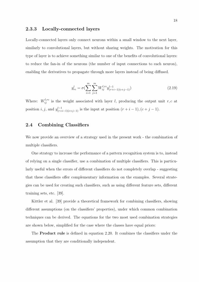
2.3.3 Locally-connected layers

Locally-connected layers only connect neurons within a small window to the next layer,

similarly to convolutional layers, but without sharing weights. The motivation for this

type of layer is to achieve something similar to one of the benefits of convolutional layers:

to reduce the fan-in of the neurons (the number of input connections to each neuron),

enabling the derivatives to propagate through more layers instead of being diffused.

ylrc = σ(m∑

i=1

m∑

j=1

Wl,rcij yl−1

(r+i−1)(c+j−1)) (2.19)

Where: Wl,rcij is the weight associated with layer l, producing the output unit r, c at

position i, j, and yl−1(r+i−1)(c+j−1) is the input at position (r + i− 1), (c+ j − 1).

2.4 Combining Classifiers

We now provide an overview of a strategy used in the present work - the combination of

multiple classifiers.

One strategy to increase the performance of a pattern recognition system is to, instead

of relying on a single classifier, use a combination of multiple classifiers. This is particu-

larly useful when the errors of different classifiers do not completely overlap - suggesting

that these classifiers offer complementary information on the examples. Several strate-

gies can be used for creating such classifiers, such as using different feature sets, different

training sets, etc. [39].

Kittler et al. [39] provide a theoretical framework for combining classifiers, showing

different assumptions (on the classifiers’ properties), under which common combination

techniques can be derived. The equations for the two most used combination strategies

are shown below, simplified for the case where the classes have equal priors:

The Product rule is defined in equation 2.20. It combines the classifiers under the

assumption that they are conditionally independent.

19

assign Z → ωj if

R∏

i=1

p(xi|ωj) =m

maxk=1

R∏

i=1

p(xi|ωk)(2.20)

In this equation, Z is the pattern being classified, ωk are the different classes, and

p(xi|ωk) is the probability assigned to class k by the classifier i.

The Sum rule is defined in equation 2.21. It combines the classifiers under the

assumption that the classifiers will not deviate dramatically from the prior probabilities.

assign Z → ωj if

R∑

i=1

p(xi|ωj) =m

maxk=1

R∑

i=1

p(xi|ωk)(2.21)

Similar to the equation above, Z is the pattern being classified, ωk are the different

classes, and p(xi|ωk) is the probability assigned to class k by the classifier i.

2.5 Transfer Learning

Transfer learning is a strategy that aims to improve the performance on a machine learning

task by leveraging knowledge obtained from a different task. The intuition is: we expect

that by learning one task we gain knowledge that could be used to learn similar tasks.

For example, learning to recognize apples might help in recognizing pears, or learning to

play the electronic organ may help learning the piano [40].

In a survey on transfer learning, Pan and Yang [40] use the following notations and

definitions for transfer learning: A domain D consists of two components: a feature

space X and a probability distribution P (X), where X = {x1, ..., xn} ∈ X . Given a

specific domain, D = {X , P (X)}, a task consist of two components: a label space Y and

an objective predictive function f(.), denoted by T = {Y , f(.)}), which is not observed,

but that can be learned from training data. The function f(.) can then be used to predict

20

the corresponding label, f(x) of a new instance x. From a probabilistic perspective, f(x)

can be written as P (y|x). In an example in the texture classification domain, we use

a feature descriptor on the textures to generate the feature space X . A given training

sample is denoted by X, X ∈ X , with associated label y, y ∈ Y . A model is then trained

on a dataset to learn the function f(.) (or P (y|x)).

With this notation, transfer learning can be defined as follows:

Definition 2.5.1 Given a source domain DS and learning task TS, a target domain DT

and learning task TT , transfer learning aims to help improve the learning of the target

predictive function fT (.) in DT using the knowledge in DS and TS, where DS 6= DT , or

TS 6= TT

To illustrate, we can use this definition for texture classification. We can apply transfer

learning by using a source task from a different domain D, for example, using a different

feature space X (with a different feature descriptor) or using a dataset with different

marginal probabilities P (X) (i.e. textures that display different properties from the target

task). We can also apply transfer learning if the task T is different: for example, using a

source task that learns different labels Y or with different objective f(.).

2.5.1 Transfer Learning in Convolutional Neural Networks

The architecture of state-of-the-art Convolutional Neural Networks (CNN) often contains

a large number of parameters, such as the network of Krizhevsky et. al for the ImageNet

dataset [26] with 60 million parameters. In this case, the weights are learned from a dataset

containing 1.2 million high-resolution images for training. However, directly learning so

many parameters from only a few thousand examples is problematic. Transfer learning

can assist in this task, by using the internal representation learned from one task, and

applying it to another task. As noted by Oquab et. al [41], a CNN can act as a generic

extractor of mid-level representations, which can be pre-trained in a source task, and then

re-used in other target tasks.

One difficulty to apply this method is that the distribution of the images, P (X), may

21

differ significantly between the source and target tasks. Oquab et. al [41] propose a

simple method to cope with this problem, by training an adaptation layer (using the

target dataset), after the convolutional layers are learned in the source task. This process

is illustrated in Fig 2.7: first a convolutional neural network is trained in the source task

(in their case the ImageNet dataset). The parameters learned by network (except for

the last layer) are then transferred to the target task (which has a smaller dataset). To

compensate for the different distribution of the images, two fully-connected layers are

added to the network, and these two layers are then trained using the target dataset.

Using this simple transfer learning procedure, Oquab et. al were able to achieve state-of-

the-art results on the competitive Pascal VOC dataset.

Figure 2.7: Transfer learning from the ImagetNet dataset to the Pascal VOC dataset

22

CHAPTER 3

STATE-OF-THE-ART

This Chapter reviews the state-of-the-art for Deep Neural Networks applied to a classifica-

tion task. Deep models were already successfully used in many domains, including several

classification tasks [33], [42], [18], natural language processing [43], acoustic modelling in

speech recognition[44] , among others. The present work is focused on texture classifica-

tion, and therefore we limited the analysis for image recognition tasks. In particular, one

object recognition problem was selected (CIFAR-10) for comparative analysis. The best

published results on this dataset are compared, and their similarities are identified.

3.1 Deep learning review on the CIFAR-10 dataset

Deep learning has been a focus of recent research, and a large variety of models have been

proposed in recent years [13]. To support the decisions on which strategies to pursue

for texture classification, a survey was conducted on the top published results in an

object recognition task: CIFAR-10 [17]. Several similarities were found in the models and

methodologies used in these papers, which provided insights for the texture classification

task. The detailed results of this analysis can be found below, and it is summarized in

the next section.

Goodfellow et al. [45] achieved the best published result on the CIFAR-10 dataset.

They used an architecture of three convolutional-layers (each followed by a max-pooling

layer), followed by one fully-connected layer, and one fully-connected softmax layer. The

key difference on this work is the usage of a new type of neuron, called Maxout, instead

of using the sigmoid function. A single maxout neuron can approximate any convex func-

tion, and in practice the maxout networks not only learn the relationships between hidden

neurons, but also the activation function of each neuron. Their model also made usage of

a regularization technique called dropout [46], which is described below. With this archi-

23

tecture, an accuracy of 90.65% was achieved in this 10-class classification problem. This

result was achieved by augmenting the training dataset with translations and horizontal

reflections, and using standard preprocessing techniques: Global contrast normalization,

and ZCA whitening.

Snoek et al. [47] used the same architecture defined by Krizhevsky in the first tests

with the CIFAR-10 dataset [17]. Considering the fact that deep networks have a significant

number of hyperparameters (such as the number of layers, and the size of each layer), they

developed a Bayesian Optimization procedure for tuning these hyperparameters. The net-

work architecture is similar to the one used by Goodfellow, with two convolutional layers,

but instead of the maxout neuron, Rectified Linear Units (RELUs) where used. Snoek et

al. started training with the best hyperparameters obtained manually (by Krizhevsky),

and used their method to fine-tune them. As a result, they were able to achieve 90.5% of

accuracy on this task, compared to 82% of accuracy obtained by Krizhevsky. Again, the

training dataset was augmented with translations and reflections to achieve this level of

accuracy.

Ciresan et al. [18] proposed a method for image classification relying on multiple deep

neural networks trained on the same data, but with different preprocessing techniques.

The networks are trained separately, and then the results are combined, by averaging

the outputs of the different networks. The architecture of the networks consisted of four

convolutional layers, followed by a fully-connected layer, and a softmax layer. Training

followed this procedure: At first, all images are preprocessed using multiple techniques,

obtaining 5 different versions of each image - they used standard image processing tech-

niques such as Histogram equalization, and Adaptive Histogram equalization. At the

beginning of each epoch, each image in the dataset is randomly translated, scaled and

rotated (i.e. the dataset is augmented). This updated dataset is then used to train the

networks. During test, the images are pre-processed with the same techniques, and the

results are combined by averaging the outputs of all networks. With this architecture, an

accuracy of 88.79% was obtained.

Zeiler and Fergus [48] propose a regularization method for convolutional networks,

24

called stochastic pooling. The most common pooling strategy, max-pooling, works by

selecting only the largest value of the pooling window. In the proposed method, a proba-

bility is assigned to each element in the window, where the larger values within the window

are given higher probabilities. One of the values is then stochastically selected using these

probabilities. At test time, the values of the window are averaged in a probabilistic form,

by multiplying the values by their probability within the window. The network architec-

ture contained three convolutional layers, each followed by stochastic pooling, and a local

response normalization layer (which normalizes the pooling outputs at each location over

a subset of neighboring feature maps). Lastly, a single fully-connected softmax layer is

used to obtain the model predictions. With this architecture, an accuracy of 84.87% was

obtained.

Hinton et al. [46] introduced a model regularization technique called dropout. The

basic idea for dropout is that for each example (or mini-batch) of training, some of the

neurons are deactivated (i.e. they are not used in the forward/back-propagation phases).

In practice this is equivalent on training an ensemble of networks containing the set of

all possible network configurations (i.e. all possible networks obtained by deactivating a

given percentage of the neurons in each layer). At test time, the full network is used, which

is equivalent to running the input in all possible network configurations, and averaging

their result. The model for the CIFAR-10 dataset contained three convolutional layers,

each followed by max-pooling and Local Response Normalization. A locally-connected

layer is used after the convolutional layers, and a 50% dropout is used in this layer. The

last layer is a softmax layer, which produces the model outputs. With this architecture,

an accuracy of 84.40% was obtained.

3.1.1 Summary of the CIFAR-10 top results

Table 3.1 provides a summary of the papers reviewed above. The most important simi-

larities among the models are the following:

1. All models used convolutional neural networks

25

2. No models used unsupervised pre-training

3. Best results used data augmentation (translation, rotation, scaling)

It is worth noting that none of top five results used unsupervised pre-training, in

spite of the fact that such models, using RBMs and autoenconders, were fundamental

for obtaining early successful results with deep learning. We can also see that the best

results used techniques that expand (augment) the original datasets, such as translations

and rotations.

26

Accuracy Algorithm Preprocessing Data Augmenta-

tion?

Pre-

training?

Architecture

90.65% [45] Deep ConvolutionalNeural Network withMaxout

- Global contrast nor-malization- ZCA whitening

Yes:- Image translations- Horizontal Reflec-tions

No CNN with:- Convolutional maxout layers with max-pooling (x3)- Fully connected maxout layer- Softmax layer

90.50% [47] Deep ConvolutionalNeural Network

Mean normalization Yes:- Image translations- Horizontal Reflec-tions

No CNN with:- Convolutional layer followed by max-poolingand local contrast normalization (x2)- Two locally connected layers- Softmax layer

88.79% [18] MCDNN (Multi-column Deep Con-volutional NeuralNetwork)

Image processing:- Image Adjustment- Histogram equaliza-tion- Adaptive HistogramEqualization- Contrast Normaliza-tion

Yes- Rotation ±5◦

- Scaling ±15%- Translation ±15%

No Several CNNs trained separately, and aver-aged in a MCDNN. CNNs are trained on datapre-processed using different techniques.- Used large number of wide layers (6 to 10layers with hundreds of maps)- Used convolutional layers, with max-pooling

84.87% [48] Deep ConvolutionalNeural Network

Mean normalization No No CNN with:- Convolutional layer followed by stochas-tic pooling and local response normalization.(x3)- Softmax layer

84.40% [46] Deep ConvolutionalNeural Network withDropout

Mean normalization No No CNN with:- Convolutional layers followed by pooling andlocal response normalization.(x3)- One locally-connected layer (where dropoutof 50% is applied)- Softmax layer

Table 3.1: Comparison of top published results on the CIFAR-10 dataset

27

CHAPTER 4

METHODOLOGY

In this Chapter we propose a methodology to train Convolutional Neural Networks on

texture classification problems. We start with a general definition on the learning process,

and introduce the texture datasets that we use to evaluate the methodology. We then

present our method for training the networks on texture problems, and the method we

use to transfer learning between tasks.

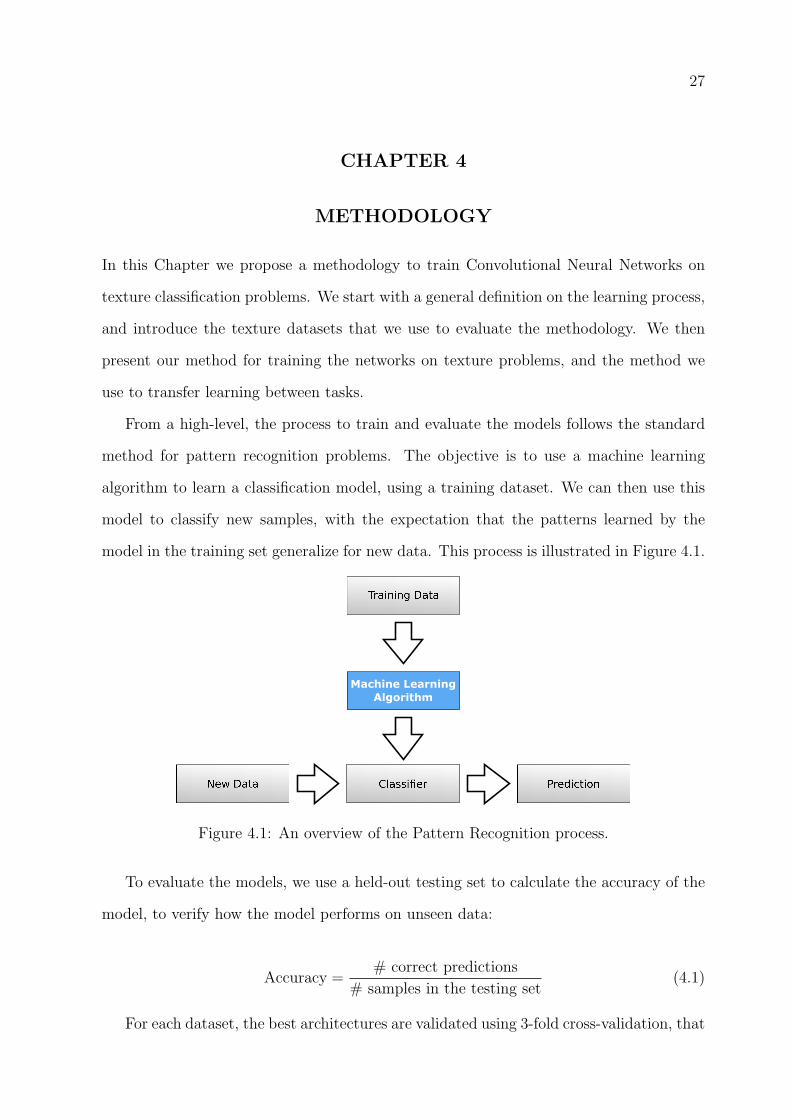
From a high-level, the process to train and evaluate the models follows the standard

method for pattern recognition problems. The objective is to use a machine learning

algorithm to learn a classification model, using a training dataset. We can then use this

model to classify new samples, with the expectation that the patterns learned by the

model in the training set generalize for new data. This process is illustrated in Figure 4.1.

Machine Learning

Algorithm

Figure 4.1: An overview of the Pattern Recognition process.

To evaluate the models, we use a held-out testing set to calculate the accuracy of the

model, to verify how the model performs on unseen data:

Accuracy =# correct predictions

# samples in the testing set(4.1)

For each dataset, the best architectures are validated using 3-fold cross-validation, that

28

is, the dataset is split three times (folds) into training, validation and testing. For each

fold, a model is trained using the training and validation sets, and tested in the testing

set. We then report the mean and standard deviation of the accuracy and compare them

with the state-of-the-art in each dataset.

4.1 Texture datasets

A total of six texture datasets were selected to evaluate the method. These datasets were

selected for two main reasons: they represent problems in different domains, and each

dataset contain different challenges for pattern recognition. Below is a description of the

selected datasets, with the different challenges that they pose. Examples of these datasets

can be found in Appendix A

4.1.1 Forest Species datasets

The first dataset contains macroscopic images for forest species recognition: pictures of

cross-section surfaces of the trees, obtained using a regular digital camera. This dataset

consists in 41 classes, containing high-resolution (3264 x 2448) images for each class. The

procedure used to collect the images, and details on the initial dataset (that contained 11

classes at the time) can be found in [49], and the full dataset in [50].

The second dataset contains microscopic images of forest species, obtained using a

laboratory procedure. This dataset consists of 112 species, containing 20 images of res-

olution 1024x768 for each class. Details on the dataset, including the procedure used to

collect the images can be found in [51]. Examples of this dataset are presented in Figure

A.2. It is worth noting that the colors on the images are not natural from the forest

species, but a result of the laboratory procedure to produce contrast on the microscopic

images. Therefore, the colors are not used for training the classifiers.

The main challenge on the two forest species datasets is the image size. Most successful

deep network models rely on small image sizes (e.g. 64x64), and these datasets contain

images that are much larger.

29

4.1.2 Writer identification

We consider two writer identification datasets. The first is the Brazilian Forensic Let-

ter Database (BFL), containing 945 images from 315 writers (3 images per writer)[52].

Hanusiak et al. [53] introduced a method to create textures from this type of image,

transforming it into a texture classification problem. This method was later explored

in depth by Bertolini [8] in two datasets: The Brazilian Forensic Letter Database, and

the IAM Database. The IAM Database was presented by Marti and Bunke[54] for offline

handwritten recognition tasks. The dataset includes scanned handwritten forms produced

by approximately 650 different writers. Samples of these datasets, and their associated

texture can be found in Figures A.4 and A.5. To allow direct comparison with published

results on these datasets, we use the same subsets of the data as Bertolini [8]. In partic-

ular, we use 115 writers from the BFL dataset, and 240 writers from the IAM dataset.

This large number of classes is the main challenge in these datasets.

4.1.3 Music genre classification

The Latin Music Dataset, introduced by Silla et al. [55] contains 3227 songs from 10

different Latin genres, and it was primarily built for the task of automatic music genre

classification. Costa et al. [56] introduced a novel approach for this task, using spec-

trograms: a visual representation of the songs. With this approach, a new dataset was

constructed, with the images (spectrograms) of the songs, enabling the usage of classic

texture classification techniques for this task.

The music genre dataset contains a property that distinguishes it from the other

datasets: on the other datasets, the textures are more homogeneous, in the sense that

patches from different parts of the image have similar characteristics. For this dataset,

however, there are differences in both axis: The music change its structure over time (X

axis), and different patterns are expected on the frequency domain (Y axis). This suggest

that convolutions can be less effective in this dataset, as patterns that are useful for one

part of the image may not be useful for other parts. The challenge is to test if convolutions

obtain good results in spite of these differences, or adapt the methodology to use a zoning

30

division, as described in the work by Costa et al. [56] and illustrated in figure 4.2.

Figure 4.2: The zoning methodology used by Costa [56].

4.1.4 Brodatz texture classification

The Brodatz album is a classical texture database, dating back to 1966, and it is widely

used for texture analysis. [57]. This dataset is composed of 112 textures, with a single

640x640 image per each texture. In order to standardize the usage of this dataset for

texture classification, Valkealahti [58] introduced the Brodatz-32 dataset, a subset of

32 textures from the Brodatz album, with 64 images per class (64x64 pixels in size),

containing patches of the original images, together with rotated and scaled versions of

them (see Figure A.6).

The challenge with the Brodatz dataset is the lower number of samples per image. In

the original Brodatz dataset, only a single image per texture is available (640x640). Since

it is common for Convolutional Networks to have large number of parameters, this type

of network usually require large datasets to be able to learn the patterns from the data.

31

4.1.5 Summary of the datasets

Table 4.1 summarizes the properties of the datasets used in this research, showing the

different challenges (in terms of number of classes, database size, etc.) as mentioned in

the previous sections.

The last column of the table counts the number of bytes used to represent the images

in a bitmap format (i.e. 1 byte per pixel for grayscale images, 3 bytes per pixel for color

images), to give a sense on the amount of information available for the classifier in each

dataset.

Dataset Num.

Classes

Num. Samples

per Class

Total Num.

of Samples

Image size Number

of bytes

Forest species(Macroscopic)

41 37 ∼ 99 2942 3264 x 2448(color)

∼65.7 GB

Forest species(Microscopic)

112 20 2240 1024 x 768 ∼1.6 GB

Music GenreClassification

10 90 900 800 x 513 ∼352 MB

Write identifica-tion (BFL)

115 27 3105 256 x 256 ∼194 MB

Write identifica-tion (IAM)

240 18 4320 128 x 256 ∼135 MB

Brodatz-32 Tex-ture classification

32 64 2048 64 x 64 ∼8 MB

Table 4.1: Summary of the properties of the datasets

4.2 Training Method for CNNs on Texture Datasets

The proposed method for training CNNs on texture datasets is outlined below. The next

sections describe the steps in further detail, and provide a rationale for the decisions.

1. Resize the images from the dataset

2. Split the dataset into training, validation and testing

3. Extract patches from the images

32

4. Train a convolutional neural network on the patches using the training and valida-

tion sets

5. Test the network on the test patches

6. Combine the patches to report results on the whole test images

4.2.1 Image resize and patch extraction

Most tasks that were successfully modeled with deep neural networks usually involve

small inputs (e.g 32x32 pixels up to 108x108 pixels). Networks with larger input sizes

contain more trainable weights requiring significant more computing power to train, and

also requiring more data to prevent overfitting.

In the case of texture classification, it is common to have access to high-resolution

texture images, and therefore we need to methods that can explore larger inputs. Instead

of simply training larger networks, we explore the hypothesis that we can classify a texture

image with only a small part of it, and train a network not on the full texture images,

but on patches of the images. This assists in reducing the size of the input to the neural

network, and also allows us to combine, for a given image, different predictions made

using patches from different parts of the image.

Besides the size of the input to the neural network, another important aspect is the size

of the filter (feature map) for the first convolutional layer. The first layer is responsible

for the first level of feature extractors, which are closely related to local features in the

image. Therefore, the filter size must be adequate for the dataset images (and vice-versa),

in the sense that relevant visual cues should be present in image patches of the size of

the filter. Considering this hypothesis, we first resize the images so that relevant visual

cues are found within windows of fixed filter sizes. We consider different filter sizes for

the first layer following the results from Coates et al. [59], that investigated the impact

of filter sizes in classification. Coates et al. empirically demonstrated that the best filter

sizes are between 5x5 and 8x8. The usage of larger filter sizes would require significantly

larger amounts of data to improve accuracy.

33

Besides this intuitive approach for choosing the filter size and the factor to resize the

images, we also explore a more systematic approach, considering both as hyperparameters

of the network, and optimizing them.

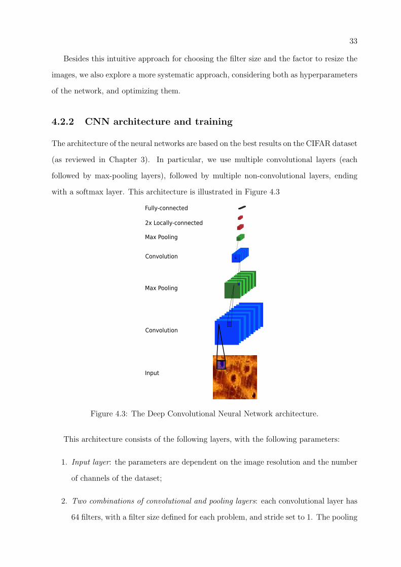
4.2.2 CNN architecture and training

The architecture of the neural networks are based on the best results on the CIFAR dataset

(as reviewed in Chapter 3). In particular, we use multiple convolutional layers (each

followed by max-pooling layers), followed by multiple non-convolutional layers, ending

with a softmax layer. This architecture is illustrated in Figure 4.3

Convolution

Convolution

Max Pooling

Max Pooling

2x Locally-connected

Fully-connected

Input

Figure 4.3: The Deep Convolutional Neural Network architecture.

This architecture consists of the following layers, with the following parameters:

1. Input layer: the parameters are dependent on the image resolution and the number

of channels of the dataset;

2. Two combinations of convolutional and pooling layers: each convolutional layer has

64 filters, with a filter size defined for each problem, and stride set to 1. The pooling

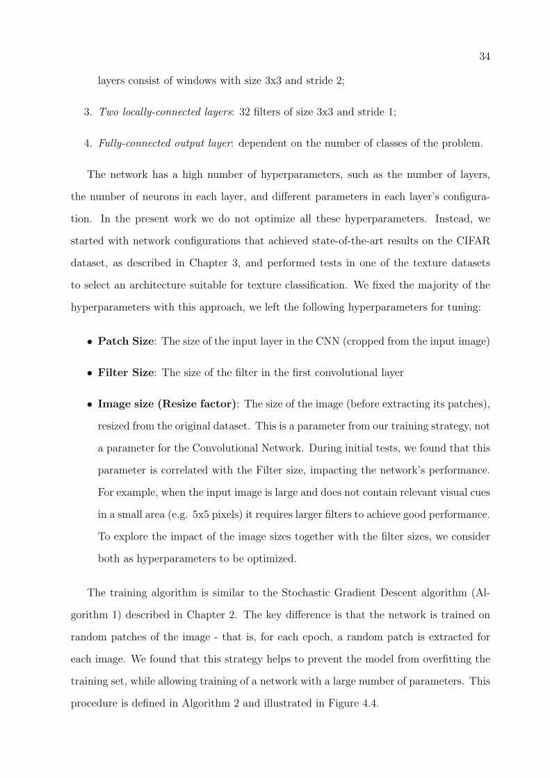
34

layers consist of windows with size 3x3 and stride 2;

3. Two locally-connected layers: 32 filters of size 3x3 and stride 1;

4. Fully-connected output layer: dependent on the number of classes of the problem.

The network has a high number of hyperparameters, such as the number of layers,

the number of neurons in each layer, and different parameters in each layer’s configura-

tion. In the present work we do not optimize all these hyperparameters. Instead, we

started with network configurations that achieved state-of-the-art results on the CIFAR

dataset, as described in Chapter 3, and performed tests in one of the texture datasets

to select an architecture suitable for texture classification. We fixed the majority of the

hyperparameters with this approach, we left the following hyperparameters for tuning:

• Patch Size: The size of the input layer in the CNN (cropped from the input image)

• Filter Size: The size of the filter in the first convolutional layer

• Image size (Resize factor): The size of the image (before extracting its patches),

resized from the original dataset. This is a parameter from our training strategy, not

a parameter for the Convolutional Network. During initial tests, we found that this

parameter is correlated with the Filter size, impacting the network’s performance.

For example, when the input image is large and does not contain relevant visual cues

in a small area (e.g. 5x5 pixels) it requires larger filters to achieve good performance.

To explore the impact of the image sizes together with the filter sizes, we consider

both as hyperparameters to be optimized.

The training algorithm is similar to the Stochastic Gradient Descent algorithm (Al-

gorithm 1) described in Chapter 2. The key difference is that the network is trained on

random patches of the image - that is, for each epoch, a random patch is extracted for

each image. We found that this strategy helps to prevent the model from overfitting the

training set, while allowing training of a network with a large number of parameters. This

procedure is defined in Algorithm 2 and illustrated in Figure 4.4.

35

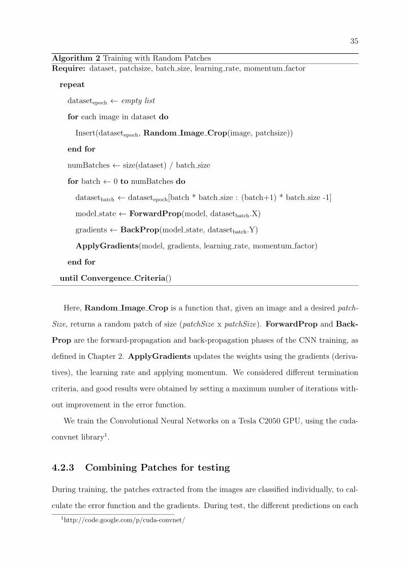
Algorithm 2 Training with Random Patches

Require: dataset, patchsize, batch size, learning rate, momentum factor

repeat

datasetepoch ← empty list

for each image in dataset do

Insert(datasetepoch, Random Image Crop(image, patchsize))

end for

numBatches ← size(dataset) / batch size

for batch ← 0 to numBatches do

datasetbatch ← datasetepoch[batch * batch size : (batch+1) * batch size -1]

model state ← ForwardProp(model, datasetbatch.X)

gradients ← BackProp(model state, datasetbatch.Y)

ApplyGradients(model, gradients, learning rate, momentum factor)

end for

until Convergence Criteria()

Here, Random Image Crop is a function that, given an image and a desired patch-

Size, returns a random patch of size (patchSize x patchSize). ForwardProp and Back-

Prop are the forward-propagation and back-propagation phases of the CNN training, as

defined in Chapter 2. ApplyGradients updates the weights using the gradients (deriva-

tives), the learning rate and applying momentum. We considered different termination

criteria, and good results were obtained by setting a maximum number of iterations with-

out improvement in the error function.

We train the Convolutional Neural Networks on a Tesla C2050 GPU, using the cuda-

convnet library1.

4.2.3 Combining Patches for testing

During training, the patches extracted from the images are classified individually, to cal-

culate the error function and the gradients. During test, the different predictions on each

1http://code.google.com/p/cuda-convnet/

36

2. Forward

Propagate

3. Back

Propagate

1. Extract random

Patches

Convolution

Convolution

Max Pooling

Max Pooling


Fully-connected

Input

Figure 4.4: The training procedure using random patches

patch that compose an image need to be combined. For each patch, the model predicts

the a posteriori probability of each class given the patch image. These probabilities are

combined following the classifier combination strategies from Kittler et al. [39], reviewed

in Chapter 2.

In the present work, we made the decision to use the set of all non-overlapping patches

from the image during test (called here Grid Patches). For each image, we extract a list

of patches, classify them all, and combine the probabilities from all patches of the image.

This procedure is described in Algorithm 3 and illustrated in Figure 4.5.

37

Algorithm 3 Testing with Grid Patches

Require: dataset, patchsize, model

PatchesDataset ← empty list

for each image in dataset do

Insert(PatchesDataset, ExtractGridPatches(image, patchSize))

end for

PatchProbabilities ← ForwardProp(model, PatchesDataset.X)

ImageProbabilities ← CombineProbabilities(PatchProbabilities)

Predictions ← argmax(ImageProbabilities)

ClassifiedCorrectly ← Count(Predictions = dataset.Y)

Accuracy ← ClassifiedCorrectly / Size(dataset)

Here, ExtractGridPatches is a function that divides an image in patches of size

(patchSize x patchSize) and returns a list of patches. ForwardProp is the forward-

propagation phase of the CNN; CombineProbabilities is a function that combines the

probabilities from all patches of each image, using either the Product Rule or Sum Rule

as defined in Chapter 2. The prediction for each sample is the class that has highest

probability among all classes. We then calculate the Accuracy as the count of correctly

classified samples, divided by the total number of samples in the testing set. When

combining the probabilities, we experimented with both combination rules, and the Sum

Rule consistently presented better results. Therefore this combination rule was used in

our experiments.

4.3 Training Method for Transfer Learning

To explore the concept of transfer learning across different texture classification tasks, we

use a procedure similar to the one used by Oquab et al. [41], but adapted to the training

procedure above that considers random patches during training.

To recall, the objective of Transfer Learning is to improve the performance in a target

task TT with a source task TS trained on a source domain DS. For example, we train a

38

2. Forward

Propagate

1. Extract all

non-overlapping

Patches

Patch Predictions

3. Combine

probabilities

Image Predictions

Convolution

Convolution

Max Pooling

Max Pooling


Fully-connected

Input

Figure 4.5: The testing procedure using non-overlapping patches

model on the IAM author identification task, and use this knowledge to improve a model

trained for the BFL author identification task.

With this objective in mind, we follow these steps:

• Train a Convolutional Neural Network in the source task

• Use this network to obtain a new representation of the target task (project the data

to another feature space)

• Use the new representation on the target task to train a new model

One interpretation for this procedure is to consider that the source task (e.g. learn a

CNN model on the IAM dataset) learn feature extractors that are generic, to some extent,

and that are useful for the target task. We use the CNN to extract a new representation

for the target dataset, which is similar to using a feature extractor to the input, obtaining

a new vector representation for each sample. When extracting the new representation,

similar to Oquab et al. [41], we use the layers of the CNN (trained on the source task)

up to the last layer before softmax. In contrast to their work, instead of training a neural

network on the new representation, we experiment with two models: logistic regression

and SVM (Support Vector Machines).

39

One challenge to apply this technique on our methodology is that, when training

the CNN, we use patches of the original images, instead of the full image. This means

that when we generate a new representation on the target dataset, we are generating

new representations for patches of the target images. The challenge is how to select the

patches from the target dataset for training. On the CNN training, we use one random

patch per epoch, but this procedure does not work well with SVM, that require a static

(fixed) dataset. To address this issue, for each image in the target dataset, we extract

the set of all non-overlapping patches (Grid Patches). This fixed dataset is then used for

training. On the test phase, we follow the same approach described above: extract the

grid patches of the dataset, and later combine the results of all patches for each image.

The algorithm for learning the new model is described in Algorithm 4 and illustrated in

Figure 4.6.

Algorithm 4 Transfer Learning - training

Require: dataset trainsource, dataset traintarget, dataset testtarget, patchSize

modelsource ← Train With Random Patches(dataset trainsource, patchSize)

Patches traintarget ← empty list

for each image in dataset traintarget do

Insert(Patches traintarget, ExtractGridPatches(image, patchSize))

end for

NewDataset traintarget ← GetNewRepresentation(modelsource, Patches traintarget)

Modeltarget ← TrainModel(NewDataset traintarget)

Here, Train With Random Patches is the training procedure described in Algo-

rithm 2; ExtractGridPatches is a function to extract all non-overlapping patches from a

image; GetNewRepresentation is a function that runs the Forward-propagation phase

of the CNN up to the last layer before Softmax, and returns the activations of the neurons

on this layer. TrainModel is a function that trains a classifier using the given dataset.

In our experiments we used a simple model (Logistic Regression) and Support Vector

Machines (SVM).

The test procedure using Transfer Learning is also adapted to the fact that we use

40

2. Forward

Propagate

(unt

-conn

ract all

non-overlapping

P (tra

epresentation

Model

rain model

Convolution

Convolution

Max Pooling

Max Pooling


Fully-connected

Input

Figure 4.6: The training procedure for transfer learning

patches of the images on the CNN model. We extract the grid patches of the target

dataset, use the model trained on the source task to generate the new representation, and

use the model trained using algorithm 4 to generate the predictions for each patch of the

image. Afterwards, we combine the results of the patches and report the accuracy. This

procedure is described in Algorithm 5 and illustrated in Figure 4.7.

Algorithm 5 Transfer Learning - test

Require: modelsource, modeltarget, dataset testtarget, patchSize

Patches testtarget ← empty list

for each image in dataset testtarget do

Insert(Patches testtarget, ExtractGridPatches(image, patchSize))

end for

NewDataset testtarget ← GetNewRepresentation(modelsource, Patches testtarget)

PatchProbabilitiestarget ← GetModelPredictions(modeltarget, NewDataset testtarget)

ImageProbabilities ← CombineProbabilities(PatchProbabilities)

Predictions ← argmax(ImageProbabilities)

ClassifiedCorrectly ← Count(Predictions = dataset testtarget.Y)

Accuracy ← ClassifiedCorrectly / Size(dataset)

41

Here, GetModelPredictions is a function on the target model (Logistic Regression

or SVM) that returns the probabilities of each class for each training example (each patch).

The remainder of the procedure follows the same steps as algorithm 3: the probabilities

of patches of each image are combined, and the accuracy is reported as the number of

correctly predicted samples divided by the number of samples in the testing set.

2. Forward

Propagate

(unt

-conn

ract all

non-overlapping

P (testin

epresentation

Model

3. Predict

P Predictions

e

probabilities

Image Predictions

Convolution

Convolution

Max Pooling

Max Pooling


Fully-connected

Input

Figure 4.7: The testing procedure for transfer learning

42

CHAPTER 5

EXPERIMENTAL RESULTS

We now present the results from experiments performed with the proposed methodology.

We start with the experiments to train a Convolutional Neural Network on each of the

texture datasets, followed by the experiments with Transfer Learning.

5.1 Forest species recognition tasks

The first experiments were conducted with the datasets for forest species classification.

The two datasets have a large number of images with high resolution, and we use the

methodology described in Chapter 4 to handle this challenge (large image sizes).

For both datasets, we first reduced the input size by resizing the images. The objective

was to ensure that discriminative visual cues could be found in small regions of the images,

enabling the model to learn discriminative patterns in the first convolutional layers.

For the Macroscopic images, we noticed that although the images are large (3264 x

2448), they are not very sharp - small regions such as 5x5 or 10x10 are blurred, and do

not have discriminative features. Based on this analysis we selected to test the following

image sizes: 326 x 244 (10% of the original) and 652 x 488 (20% of the original).

For the microscopic images, the images are smaller (1024 x 768), and they are already

crisp. For this dataset, however, we noticed that some textures are not homogeneous

- for example, some samples contain large holes, that could only be captured by either

using much large filters, or by resizing the image to smaller sizes. We explore this idea by

training models with the following image sizes: 307 x 230 (30%), 512 x 384 (50%), 716 x

537 (70%) and 1024 x 768 (100%).

For each dataset and for each configuration of the hyperparameters, we trained one

Convolutional Neural Network following the methodology from Chapter 4 and calculated

the accuracy. For the dataset with Macroscopic images, training a model took about

43

1.2 hours, and for the dataset with Microscopic images, training took close to 3h. The

following sections review the results.

5.1.1 Classification rates

Figure 5.1 summarizes the error rates (number of misclassified samples divided by the total

number of samples) on the Macroscopic dataset, for each CNN trained with a particular

set of hyperparameters. The table on the left summarizes the results of the networks

trained on images resized to 10% (326 x 244), and the table on the right summarizes the

results of the networks trained on images resized to 20% (652 x 488). For each table, we

have one entry for each combination of Patch Size and Filter Size (size of the filter on

the first convolutional layer). The color of the cell indicates the error - lower error rates

(better models) are displayed in lighter colors.

Figure 5.1: Error rates on the Forest Species dataset with Macroscopic images, for CNNstrained with different hyperparameters.

The model with lowest error rate was the model trained on the dataset resized to 10%

of the original size, using the smallest patch (32x32) and the largest filter size (12x12).

This model obtained an error rate of 3.22% (or, equivalently, an accuracy of 96.78%).

It is worth noting that, during test, we extract the set of non-overlapping patches from

the images and combine the results. This means that using large patch sizes implies in

44

dividing an image in less patches. For example, for patches of size 32x32, the image is

divided in 70 patches, while for the 96x96 patches, the image is divided in 6 patches.

Figure 5.2 summarizes the error rates on the Microscopic dataset, for each CNN trained

with a particular set of hyperparameters:

Figure 5.2: Error rates on the Forest Species dataset with Microscopic images, for CNNstrained with different hyperparameters.

For this dataset, the model with lowest error rate was trained on the dataset with

the images resized to 30% of the original size, with Patch Size 32x32 and filter size 5x5.

We noticed that the models trained on the images with original size performed poorly

compared to models trained on reduced images. Even though the visual analysis of the

original image suggested that small regions already contained relevant visual cues, these

45

may not be useful (discriminative) features for the model, supporting the argument that

it is better to consider the image size as a hyperparameter and run models with different

image sizes.

Figure 5.3 shows the predictions of a model trained on the Macroscopic images. A total

of eight random patches from the testing set are displayed, with the top 4 classes predicted

by the model (that is, the classes with higher probability according to the model). In this

figure, the sizes of the horizontal bars are the probability assigned for the sample to a

particular class, and the bar in the color red is the correct label (also displayed below the

image). For ease of understanding, the classes were numbered (from 0 to 40) instead of

using the names of the trees. We can see that the model predicts with high confidence

the majority of the samples.

Figure 5.3: Random predictions for patches on the Testing set (Macroscopic images)

Figure 5.4 displays the predictions of a model trained on the Microscopic images.

Similarly with the case for the Macroscopic dataset, we see that the model often provides

high confidence on the probabilities. Unfortunately, this is the case even when the model

is incorrect on the prediction (for example the image of class 92, misclassified as class 57).

46

Figure 5.4: Random predictions for patches on the Testing set (Microscopic images)

5.1.2 Feature Learning

As discussed in Chapter 1, one of the advantages of using deep learning techniques is

not requiring the design of feature extractors, but instead let the model learn them. It

is possible to visualize the feature detectors that model learn on the first convolutional

layer, considering the weights on the learned filters (feature maps). Figure 5.5 displays

the filters that were learned in the first convolutional layer for the networks trained on

the macroscopic images dataset. In this figure, we consider the networks trained on the

images resized to 10% of the original (326 x 244), with small patch sizes (32x32) and

large patch sizes (96x96). We can observe that in the majority of the cases the networks

learn interesting feature detectors, some similar to edge detectors, others capturing color

changes, and other filters that look particular to this dataset (such as the ones that

resemble small holes in the woods). We can also observe that larger filter sizes seem

to work better (i.e. learn more interesting features) with large patch sizes. However,

considering that the performance with large patches is worse (as seen in Figure 5.1) we

can infer that although using larger patch sizes helps in classifying each patch, it does not

compensate the fact that we have fewer patches to combine in the final image.

Figure 5.6 contains the features learned in the first convolutional layer for the network

that presented best results on the Microscopic images dataset. The network was trained

47

3x3

32x32

P

F

Figure 5.5: Filters learned by the first convolutional layers of models trained on theMacroscopic images dataset.

on images of size 308 x 230 (30% of the original), with filter size 5 and patch size 32.

Figure 5.6: Filters learned by the first convolutional layer of a model trained on theMicroscopic images dataset.

5.1.3 Comparison with the state of the art

The dataset with Macroscopic images has been analyzed and tested using texture classifi-

cation techniques by Paula et al. in [50], [5] and [60]. The best results were achieved with a

combination of multiple SVM classifiers trained with different texture feature descriptors:

GLCM, LBP, CLBP and color-based features (color histograms).

48

Table 5.1 summarizes the result of the convolutional neural network trained on the

macroscopic dataset, and compares it with the current state-of-the-art on this dataset. We

can see that the convolutional neural network achieves state-of-the-art results compared

with previous results with a single classifier, and reaches close to the best published

result, that uses a combination of 6 different classifiers (trained with CLBP (x2), LBP,

Gabor-filters, Fractals and Color-based features).

Table 5.1: Classification on the Macroscopic images dataset

Features and Algorithm Accuracy

LBP (SVM) [60] 85.84%Color-based features (SVM) [60] 87.53%

Gabor filters (SVM) [60] 87.66%CLBP (SVM) [60] 96.22%

Multiple classifiers (SVM) [60] 97.77%Proposed method (CNN) 96.24% (+- 0.27%)

On the Microscopic images dataset, the best published result is from Cavalin et al.

[61]. Cavalin et al. trained SVM classifiers using GLCM, LBP and LPQ features. The

best result was achieved by a combination of the LPQ and GLCM features, achieving

93.2% of accuracy in the 112-class problem.

Table 5.2 summarizes the result of the convolutional neural network trained on the

microscopic dataset. The proposed model outperforms the best published results on this

dataset by a large margin:

Table 5.2: Classification on the Microscopic images dataset


LBP (SVM) [51] 86.00%GLCM (SVM) [61] 80.70%LBP (SVM) [61] 88.50%LPQ (SVM) [61] 91.50%

LPQ + GLCM (SVM) [61] 93.20%Proposed method (CNN) 98.16% (+- 0.37%)

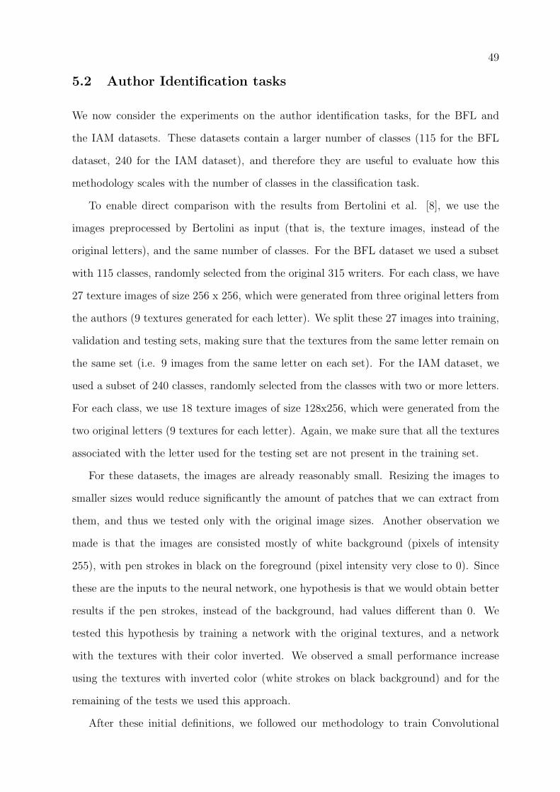
49

5.2 Author Identification tasks

We now consider the experiments on the author identification tasks, for the BFL and

the IAM datasets. These datasets contain a larger number of classes (115 for the BFL

dataset, 240 for the IAM dataset), and therefore they are useful to evaluate how this

methodology scales with the number of classes in the classification task.

To enable direct comparison with the results from Bertolini et al. [8], we use the

images preprocessed by Bertolini as input (that is, the texture images, instead of the

original letters), and the same number of classes. For the BFL dataset we used a subset

with 115 classes, randomly selected from the original 315 writers. For each class, we have

27 texture images of size 256 x 256, which were generated from three original letters from

the authors (9 textures generated for each letter). We split these 27 images into training,

validation and testing sets, making sure that the textures from the same letter remain on

the same set (i.e. 9 images from the same letter on each set). For the IAM dataset, we

used a subset of 240 classes, randomly selected from the classes with two or more letters.

For each class, we use 18 texture images of size 128x256, which were generated from the

two original letters (9 textures for each letter). Again, we make sure that all the textures

associated with the letter used for the testing set are not present in the training set.

For these datasets, the images are already reasonably small. Resizing the images to

smaller sizes would reduce significantly the amount of patches that we can extract from

them, and thus we tested only with the original image sizes. Another observation we

made is that the images are consisted mostly of white background (pixels of intensity

255), with pen strokes in black on the foreground (pixel intensity very close to 0). Since

these are the inputs to the neural network, one hypothesis is that we would obtain better

results if the pen strokes, instead of the background, had values different than 0. We

tested this hypothesis by training a network with the original textures, and a network

with the textures with their color inverted. We observed a small performance increase

using the textures with inverted color (white strokes on black background) and for the

remaining of the tests we used this approach.

After these initial definitions, we followed our methodology to train Convolutional

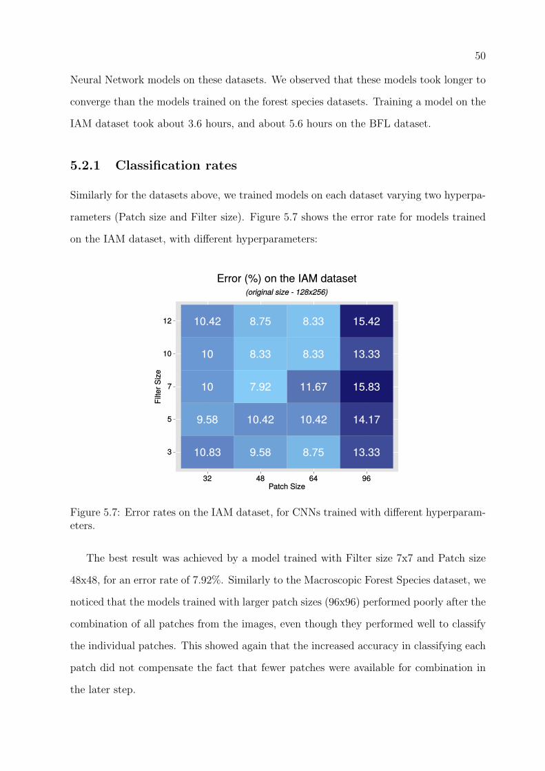
50

Neural Network models on these datasets. We observed that these models took longer to

converge than the models trained on the forest species datasets. Training a model on the

IAM dataset took about 3.6 hours, and about 5.6 hours on the BFL dataset.


Similarly for the datasets above, we trained models on each dataset varying two hyperpa-

rameters (Patch size and Filter size). Figure 5.7 shows the error rate for models trained

on the IAM dataset, with different hyperparameters:

Figure 5.7: Error rates on the IAM dataset, for CNNs trained with different hyperparam-eters.

The best result was achieved by a model trained with Filter size 7x7 and Patch size

48x48, for an error rate of 7.92%. Similarly to the Macroscopic Forest Species dataset, we

noticed that the models trained with larger patch sizes (96x96) performed poorly after the

combination of all patches from the images, even though they performed well to classify

the individual patches. This showed again that the increased accuracy in classifying each

patch did not compensate the fact that fewer patches were available for combination in

the later step.

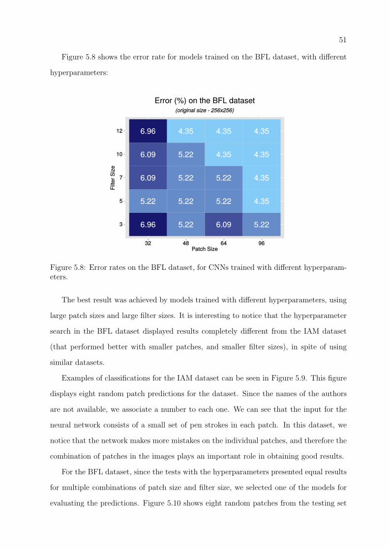
51

Figure 5.8 shows the error rate for models trained on the BFL dataset, with different

hyperparameters:

Figure 5.8: Error rates on the BFL dataset, for CNNs trained with different hyperparam-eters.

The best result was achieved by models trained with different hyperparameters, using

large patch sizes and large filter sizes. It is interesting to notice that the hyperparameter

search in the BFL dataset displayed results completely different from the IAM dataset

(that performed better with smaller patches, and smaller filter sizes), in spite of using

similar datasets.

Examples of classifications for the IAM dataset can be seen in Figure 5.9. This figure

displays eight random patch predictions for the dataset. Since the names of the authors

are not available, we associate a number to each one. We can see that the input for the

neural network consists of a small set of pen strokes in each patch. In this dataset, we

notice that the network makes more mistakes on the individual patches, and therefore the

combination of patches in the images plays an important role in obtaining good results.

For the BFL dataset, since the tests with the hyperparameters presented equal results

for multiple combinations of patch size and filter size, we selected one of the models for

evaluating the predictions. Figure 5.10 shows eight random patches from the testing set

52

Figure 5.9: Random predictions for patches on the IAM Testing set

of the BFL dataset in the model with patch size 64x64 and filter size 10x10. Again we

see the model making several mistakes when classifying the patches, but from the results

after the combination of all patches for an author’s letter we see that the combination of

patches minimizes the number of errors.

Figure 5.10: Random predictions for patches on the BFL Testing set

53


Figures 5.11 and 5.12 shows the filters learned by the first convolutional layers in the IAM

and BFL datasets respectively. We can see very similar feature detectors learned by the

two networks, with several filters that learned how to capture small parts of a pen stroke:

horizontal, vertical and diagonal straight lines, as well as some curved lines.

Figure 5.11: Filters learned by the first convolutional layer of a model trained on the IAMdataset.

Figure 5.12: Filters learned by the first convolutional layer of a model trained on the BFLdataset.


Table 5.3 compares the results above with the best published result on the IAM dataset.

For this dataset, the best results were presented by Bertolini et al. [8]. We compare our

results with the writer-dependent approach from Bertolini et al., as their results using

a dissimilarity framework (a writer-independent approach) are not directly comparable.

We can see that the proposed method outperforms the previous result on this dataset.

Table 5.3: Classification on the IAM datasetFeatures and Algorithm Accuracy

LPQ (SVM) [8] 88.30%Proposed method (CNN) 91.39% (+- 0.51%)

Table 5.4 compares the results of the proposed method with the best published result

on the BFL dataset. For this dataset, the best results were presented by Bertolini et al.

54

[8]. Again, we compare our proposed method with the writer-dependent approach from

Bertolini et al. (i.e. without using dissimilarity). For this dataset, the proposed method

with a CNN performs worse than the state-of-the-art.

Table 5.4: Classification on the BFL datasetFeatures and Algorithm Accuracy

LPQ (SVM) [8] 98.26%Proposed method (CNN) 95.36% (+- 0.41%)

5.3 Music Genre classification task

This section describes the results on the Latin Music Dataset. For this experiment we

use the dataset processed by Costa et al. [56] instead of the original song fragments,

that is, we use the spectrograms generated from each sample as input to our classifier.

These images present a challenge compared to the datasets used above, since these are not

homogeneous textures: we observe that the textures have different patterns in different

regions of the image, as we move in the X axis (time) or the Y axis (frequency) in the

spectrogram. We applied the proposed method on this dataset, and the results were

poor. Initial experiments achieve an accuracy of 54% on the testing set, which is a poor

result for a classification task with only 10 classes. This result can be justified by the fact

that our method does not consider the location of each patch during classification, and

therefore it works best when the texture presents similar patterns across the image.

After these initial tests, we attempted the same zoning strategy as Costa et al. [56].

The approach is to partition the image in both axis (time and frequency), and train a

classifier for each part. We split our image in three parts in the X axis (time) and in

10 parts in the Y axis (frequency), giving a total of 30 regions. For each region, we

trained a Convolution Neural Network following the proposed methodology. During test,

we split the images from the testing set into these 30 regions, obtain the predictions from

each network, and combine the results of the 30 classifiers, following again the classifier

combination strategies from Kittler et al. [39], reviewed in Chapter 2. Again, we obtained

better results with the Sum Rule for combining the classifiers. Each of the 30 networks

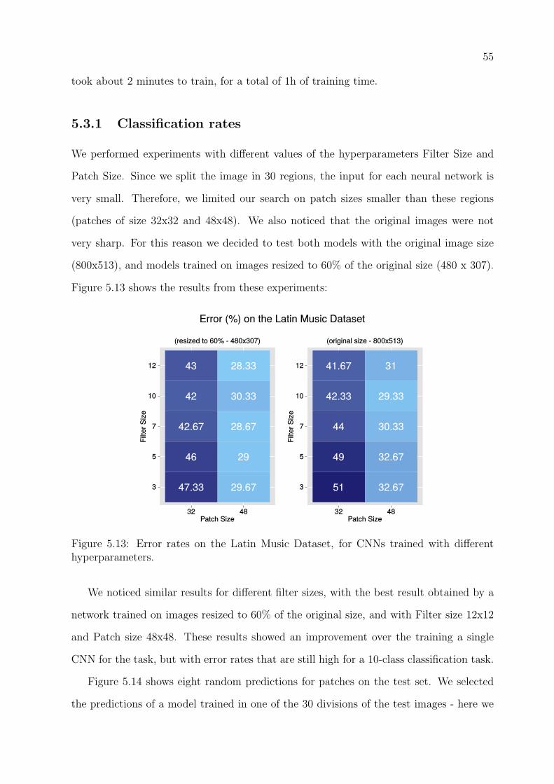
55

took about 2 minutes to train, for a total of 1h of training time.


We performed experiments with different values of the hyperparameters Filter Size and

Patch Size. Since we split the image in 30 regions, the input for each neural network is

very small. Therefore, we limited our search on patch sizes smaller than these regions

(patches of size 32x32 and 48x48). We also noticed that the original images were not

very sharp. For this reason we decided to test both models with the original image size

(800x513), and models trained on images resized to 60% of the original size (480 x 307).

Figure 5.13 shows the results from these experiments:

Figure 5.13: Error rates on the Latin Music Dataset, for CNNs trained with differenthyperparameters.

We noticed similar results for different filter sizes, with the best result obtained by a

network trained on images resized to 60% of the original size, and with Filter size 12x12

and Patch size 48x48. These results showed an improvement over the training a single

CNN for the task, but with error rates that are still high for a 10-class classification task.

Figure 5.14 shows eight random predictions for patches on the test set. We selected

the predictions of a model trained in one of the 30 divisions of the test images - here we

56

show the predictions on the region (6, 1) - that is, the region corresponding to row 6 (on

the Y axis) and column 1 (on the X axis). We can see that the model is not very reliable

on its predictions, except on a few cases.

Figure 5.14: Random predictions for test patches on the Latin Music Dataset


Figure 5.15 displays the filters learned by the first convolutional layer of the model trained

in region (6, 1). The model seems to learn the patterns present on the histogram, but

from the experimental results we can infer that these patterns are not very discriminative

for the task.

Figure 5.15: Filters learned by the first convolutional layer of a model trained on theLatin Music dataset.

57


Table 5.5 compares the result of the proposed method with the best published results.

For this dataset, Costa et al. used SVM classifiers with LBP (Local Binary Patterns) to

obtain the best results. Using this type of classifier with zoning strategies, a classification

accuracy of 82.33% was obtained. The accuracy with the proposed method did not match

the state-of-the-art for this task. One potential reason for the poor performance is the

fact that each CNN trained for this dataset has little data available (since we are dividing

the images in 30 parts and training a network in each part) - analyzing the filters learned

by the models, it seems that they were not able to learn discriminative features. It is

also worth noting that, during the 3-fold validation, we identified a larger variance in the

classification performance, compared to the CNNs in other tasks.

Table 5.5: Classification on the Latin Music datasetFeatures and Algorithm Accuracy

LPQ + Gabor Filters (SVM) [9] 80.78% (+- 0.77)LBP (SVM) [56] 82.33% (+- 1.45)

Proposed method (CNN) 73.67% (+- 1.41%)

We now compare the errors committed by the proposed method (CNN) with errors

made by the model from Costa et al. [9]). The objective is to identify if the models

commit similar types of errors, or if they present different types of errors - suggesting

that the two models offer complementary information.

Table 5.6 shows the confusion matrix of our model (the combination of CNNs trained

in segments of the image). In this table, the rows contain the actual (true) labels, and the

columns contain the predictions. Each cell contains the percentage of the samples of the

actual class (row) that were predicted as a particular class (column). Table 5.7 contains

the same type of information, for the results published by Costa et al. Comparing the two

tables, we see that in most cases the types of errors are similar. In few cases the proposed

method performs better - in the classification of class 9 (Tango) overall, for mistakes

between class 0 (Axe) and class 6 (Pagode); mistakes between class 8 (Sertaneja) and

class 4 (Gaucha), among others. With this comparison, we expect that the combination

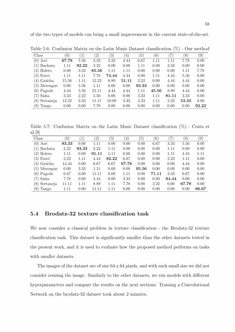
58

of the two types of models can bring a small improvement in the current state-of-the-art.

Table 5.6: Confusion Matrix on the Latin Music Dataset classification (%) - Our method

Class (0) (1) (2) (3) (4) (5) (6) (7) (8) (9)(0) Axe 67.78 5.56 3.33 2.22 4.44 6.67 1.11 1.11 7.78 0.00(1) Bachata 1.11 92.22 2.22 0.00 0.00 1.11 0.00 3.33 0.00 0.00(2) Bolero 0.00 3.33 85.56 1.11 1.11 0.00 0.00 0.00 1.11 7.78(3) Forro 1.11 1.11 7.78 74.44 4.44 0.00 1.11 4.44 5.56 0.00(4) Gaucha 15.56 1.11 12.22 8.89 51.11 2.22 0.00 4.44 4.44 0.00(5) Merengue 0.00 5.56 1.11 0.00 0.00 93.33 0.00 0.00 0.00 0.00(6) Pagode 4.44 5.56 21.11 4.44 4.44 1.11 45.56 8.89 4.44 0.00(7) Salsa 3.33 2.22 5.56 0.00 0.00 3.33 1.11 81.11 3.33 0.00(8) Sertaneja 12.22 3.33 11.11 10.00 3.33 3.33 1.11 2.22 53.33 0.00(9) Tango 0.00 0.00 7.78 0.00 0.00 0.00 0.00 0.00 0.00 92.22

Table 5.7: Confusion Matrix on the Latin Music Dataset classification (%) - Costa etal.[9]

Class (0) (1) (2) (3) (4) (5) (6) (7) (8) (9)(0) Axe 83.33 0.00 1.11 0.00 0.00 0.00 6.67 3.33 5.56 0.00(1) Bachata 2.22 93.33 2.22 1.11 0.00 0.00 0.00 1.11 0.00 0.00(2) Bolero 1.11 0.00 91.11 1.11 0.00 0.00 0.00 1.11 4.44 1.11(3) Forro 2.22 1.11 4.44 82.22 6.67 0.00 0.00 2.22 1.11 0.00(4) Gaucha 14.44 0.00 6.67 6.67 67.78 0.00 0.00 0.00 4.44 0.00(5) Merengue 0.00 3.33 1.11 0.00 0.00 95.56 0.00 0.00 0.00 0.00(6) Pagode 6.67 0.00 11.11 0.00 1.11 0.00 71.11 3.33 6.67 0.00(7) Salsa 7.78 0.00 4.44 0.00 3.33 0.00 0.00 84.44 0.00 0.00(8) Sertaneja 11.11 1.11 8.89 1.11 7.78 0.00 2.22 0.00 67.78 0.00(9) Tango 1.11 0.00 11.11 1.11 0.00 0.00 0.00 0.00 0.00 86.67

5.4 Brodatz-32 texture classification task

We now consider a classical problem in texture classification - the Brodatz-32 texture

classification task. This dataset is significantly smaller than the other datasets tested in

the present work, and it is used to evaluate how the proposed method performs on tasks

with smaller datasets.

The images of the dataset are of size 64 x 64 pixels, and with such small size we did not

consider resizing the image. Similarly to the other datasets, we run models with different

hyperparameters and compare the results on the next sections. Training a Convolutional

Network on the brodatz-32 dataset took about 2 minutes.

59


Figure 5.16 reports the error rates of the models trained on different hyperparameters.

Figure 5.16: Error rates on the Brodatz dataset, for CNNs trained with different hyper-parameters.

It is worth noting that for patches of size 48x48 and 64x64 we have only a single patch

to classify the image, where patches of size 32x32 allowed the combination of 4 patches on

each test image. The model with best performance was trained with Filter size of 3x3 and

Patch size of 32x32. It is also interesting to observe that the models trained with patches

of size 48x48 performed better than the patches of size 64x64, in spite of the fact that

only a single patch is available per test image (in both cases). One hypothesis for this

result is that, in the model trained with 48x48 patches, we use random patches during

training, which may reduce the overfitting on the training data. We cannot use random

patches for the model trained with 64x64 patches, since the images themselves are of size

64x64.

Figure 5.17 displays eight random patches from the testing set, from the network that

obtained the best results above. Again, the image displays the probability assigned by

the model to different classes (the 4 classes with higher probability), and the bar in red

indicates the correct label (also shown below the image).

60

Figure 5.17: Random predictions for patches on the Brodatz-32 Testing set


The filters learned by the first convolutional layer are displayed in Figure 5.18. In this

case, we can see that only a few filters learned relevant features, while many of them

remained very homogeneous (almost completely gray), and very redundant. This is likely

due to low amount of data in the training set for this task.

Figure 5.18: Filters learned by the first convolutional layer of a model trained on theBrodatz-32 dataset.


Table 5.8 compare our results with the best published results in the Brodatz-32 task. The

best published result for the Brodatz-32 dataset is from Chen [62] achieving 98.9% of

accuracy on the 32-class classification problem using a novel LBP operator called Robust

Local Binary Pattern. For this task, the proposed method achieves inferior results, with

a mean accuracy of 91.27%.

61

Table 5.8: Classification on the Brodatz-32 datasetFeatures and Algorithm Accuracy

Gabor filters (KNN) [62] 95.8%Multiple texture descriptors (Decision Trees) [63] 96.5%

Dominant LBP (KNN) [62] 98.30%Robust LBP (KNN) [62] 98.90%Proposed method (CNN) 91.27% (+- 0.53%)

5.5 Transfer Learning

We now present the results of our experiments with Transfer Learning. As presented in

Chapter 4, our objective is to use one dataset to train a Convolutional Neural Network,

and transfer knowledge to another task, seeking to improve the results on it.

For each experiment, we follow the procedure defined in Chapter 4: we first trained

a Convolutional Neural Network on the source task, using the best hyperparameters

from the results above. Then we use this model to obtain a new representation of the

target dataset, projecting the samples to another feature space. Finally, we use this

new representation of the target dataset to train a model. In these experiments, we

trained Logistic Regression models and Support Vector Machines (SVMs). For the SVM

training, we use the python package scikit-learn [64], that provides a wrapper over the

libsvm [65] library. We train SVMs with the radial basis function (RBF) kernel, selecting

the hyperparameters C and γ using a grid search, following the recommended values from

Hsu [66]. It is worth noting that due to limitations on computing power, we do not

optimize these hyperparameters using the whole training set. Instead, a subset of five

thousand examples is randomly selected to perform this optimization, and subsequently

an SVM is trained with these hyperparameters on the whole training set. We then test

the model once in the testing set, and report the results.

5.5.1 Tasks from similar domains

We first present the results of transferring learning across tasks with similar domains.

In particular, we selected two tests to perform: transfer learning across tasks on For-

est species recognition (using the Microscopic and Macroscopic datasets), and transfer

62

learning across tasks on author identification (using the IAM and BFL datasets).

The first experiment involved the datasets for Forest species recognition. We used

the dataset of Microscopic images to train a CNN, seeking to improve the performance

on the task of recognizing the species from Macroscopic images. The results from this

experiment are presented in Table 5.9.

Table 5.9: Classification on the Macroscopic Forest species dataset(using CNN trained on the Microscopic Forest species dataset)


Multiple classifiers (SVM) [60] 97.77%Proposed method (CNN) 96.24%

Transfer Learning (Logistic Regression) 93.76%Transfer Learning (SVM) 95.55%

The best result using transfer learning achieved an accuracy of 95.55%, close to the

best result obtained by training a CNN on the Macroscopic images dataset (96.24%). This

suggests that, even though the images from both datasets look very different, the features

learned for the dataset with Microscopic images were discriminative for the dataset with

Macroscopic images. In particular, we can see that the result of Logistic Regression (a

linear classifier) was reasonably high, and therefore the CNN (trained on the Microscopic

dataset) is able to project the data from the Macroscopic dataset to a feature space where

the classes are (almost) linearly separable.

For the second experiment with this strategy, we used a CNN trained on the IAM

dataset, seeking to improve the results on the BFL dataset. The results for this experiment

are presented in Table 5.10.

Table 5.10: Classification on the BFL dataset(using CNN trained on the IAM dataset)


LPQ (SVM) [8] 98.26%Proposed method (CNN) 95.36%


This experiment resulted in two interesting and unexpected results. Using Transfer

Learning we were able to obtain a superior accuracy on the BFL dataset, compared

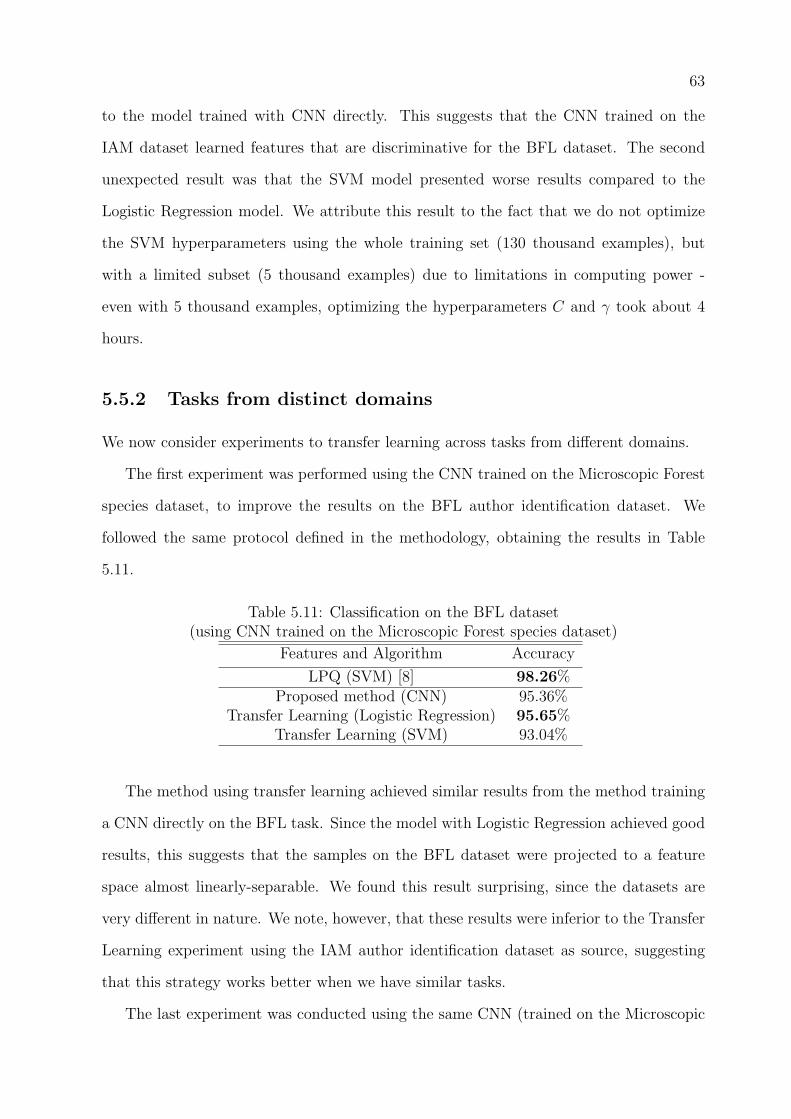
63

to the model trained with CNN directly. This suggests that the CNN trained on the

IAM dataset learned features that are discriminative for the BFL dataset. The second

unexpected result was that the SVM model presented worse results compared to the

Logistic Regression model. We attribute this result to the fact that we do not optimize

the SVM hyperparameters using the whole training set (130 thousand examples), but

with a limited subset (5 thousand examples) due to limitations in computing power -

even with 5 thousand examples, optimizing the hyperparameters C and γ took about 4

hours.

5.5.2 Tasks from distinct domains

We now consider experiments to transfer learning across tasks from different domains.

The first experiment was performed using the CNN trained on the Microscopic Forest

species dataset, to improve the results on the BFL author identification dataset. We

followed the same protocol defined in the methodology, obtaining the results in Table

5.11.

Table 5.11: Classification on the BFL dataset(using CNN trained on the Microscopic Forest species dataset)


LPQ (SVM) [8] 98.26%Proposed method (CNN) 95.36%


The method using transfer learning achieved similar results from the method training

a CNN directly on the BFL task. Since the model with Logistic Regression achieved good

results, this suggests that the samples on the BFL dataset were projected to a feature

space almost linearly-separable. We found this result surprising, since the datasets are

very different in nature. We note, however, that these results were inferior to the Transfer

Learning experiment using the IAM author identification dataset as source, suggesting

that this strategy works better when we have similar tasks.

The last experiment was conducted using the same CNN (trained on the Microscopic

64

Forest species dataset) to increase the performance on the Brodatz-32 task. The results

are presented in Table 5.12.

Table 5.12: Classification on the Brodatz-32 dataset(using CNN trained on the Microscopic Forest images dataset)


Robust LBP (KNN) [62] 98.90%Proposed method (CNN) 91.27%


For this dataset, we could see a large increase in classification rate using the transfer

learning method. This is likely due to the fact that the Brodatz-32 dataset is very small,

and the CNN trained directly on it was unable to learn good representations. Even though

the samples from the two datasets are very different, we can see that the representations

learned by the CNN trained on the Microscopic Forest images dataset were relevant for the

Brodatz-32 task. Considering the results on the experiments with the author identification

datasets, we would expect even better results if the source task (used to train a CNN)

was closer to the Brodatz-32 dataset, for example, a larger dataset of natural textures.

65

CHAPTER 6

CONCLUSION

The task of texture classification has relevant applications in a wide range of domains, and

although being successful in many areas, it is still object of active research with potential

to increase classification rates.

We developed a simple method to use Convolutional Neural Networks for texture clas-

sification, based on the methods used for object recognition, but taking advantage of

the properties particular to texture classification. Our tests with six texture classifica-

tion datasets demonstrated that this method is able to achieve state-of-the-art results in

scenarios where large amounts of data are available, which is the case of many texture

datasets (where large images are used).

We also presented a transfer learning method for texture classification using Convo-

lutional Neural Networks, allowing the usage of a dataset from one classification task to

improve the classification performance on other tasks. Our experiments with this strat-

egy showed improved accuracy when using datasets from similar tasks. The experiments

also demonstrated that this method can be used to improve the performance on tasks

where the dataset is very small, by leveraging the knowledge learned by other texture

classification tasks, even if they are not very similar.

Future work can explore the optimization of the hyperparameters on the convolutional

network (such as number of layers, number of neurons per layer, etc.), since these hyper-

paramenters were fixed during the experiments on the present work. The strategy to

extract patches during testing can also be further explored, experimenting with different

strategies such as random patch extraction.

66

APPENDIX A

SAMPLE IMAGES ON THE DATASETS

As reviewed in Chapter 3, a total of six datasets were selected for this work. The datasets

were selected to represent distinct domains, and to present different challenges for training.

The figures below contain samples of each dataset:

Figure A.1: Sample images from the macroscopic Brazilian forest species dataset

67

Figure A.2: Sample images from the microscopic Brazilian forest species dataset

Figure A.3: Sample texture created from the Latin Music Dataset dataset.

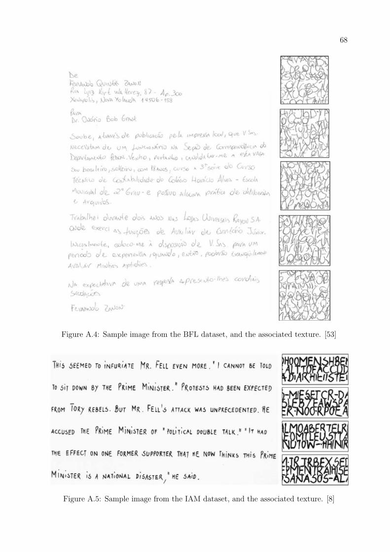
68

Figure A.4: Sample image from the BFL dataset, and the associated texture. [53]

Figure A.5: Sample image from the IAM dataset, and the associated texture. [8]

69

Figure A.6: Sample images from the Brodatz-32 dataset [58]

70

BIBLIOGRAPHY

[1] H. Harms, U. Gunzer, and H. M. Aus, “Combined local color and texture analysis

of stained cells,” Computer Vision, Graphics, and Image Processing, vol. 33, no. 3,

pp. 364–376, Mar. 1986.

[2] A. Khademi and S. Krishnan, “Medical image texture analysis: A case study with

small bowel, retinal and mammogram images,” in Canadian Conference on Electrical

and Computer Engineering, 2008. CCECE 2008, May 2008, pp. 001 949–001 954.

[3] R. Sutton and E. L. Hall, “Texture measures for automatic classification of pulmonary

disease,” IEEE Transactions on Computers, vol. C-21, no. 7, pp. 667–676, Jul. 1972.

[4] J. Y. Tou, Y. Tay, and P. Y. Lau, “A comparative study for texture classification

techniques on wood species recognition problem,” in Fifth International Conference

on Natural Computation, 2009. ICNC ’09, vol. 5, 2009, pp. 8–12.

[5] P. Filho, L. Oliveira, A. Britto, and R. Sabourin, “Forest species recognition using

color-based features,” in 2010 20th International Conference on Pattern Recognition

(ICPR), 2010, pp. 4178–4181.

[6] M. Nasirzadeh, A. Khazael, and M. bin Khalid, “Woods recognition system based

on local binary pattern,” in 2010 Second International Conference on Computational

Intelligence, Communication Systems and Networks (CICSyN), 2010, pp. 308–313.

[7] R. Haralick, K. Shanmugam, and I. Dinstein, “Textural features for image classifica-

tion,” IEEE Transactions on Systems, Man and Cybernetics, vol. SMC-3, no. 6, pp.

610–621, Nov. 1973.

[8] D. Bertolini, L. S. Oliveira, E. Justino, and R. Sabourin, “Texture-based descriptors

for writer identification and verification,” Expert Systems with Applications, 2012.

71

[9] Y. M. Costa, L. S. Oliveira, A. L. Koerich, F. Gouyon, and J. G. Martins, “Music

genre classification using LBP textural features,” Signal Processing, vol. 92, no. 11,

p. 27232737, 2012.

[10] C. M. Bishop and N. M. Nasrabadi, Pattern recognition and machine learning.

springer New York, 2006, vol. 1.

[11] J. Zhang and T. Tan, “Brief review of invariant texture analysis methods,” Pattern

recognition, vol. 35, no. 3, p. 735747, 2002.

[12] Y. Guo, G. Zhao, and M. Pietikinen, “Discriminative features for texture descrip-

tion,” Pattern Recognition, vol. 45, no. 10, pp. 3834–3843, Oct. 2012.

[13] Y. Bengio, “Learning deep architectures for AI,” Foundations and trends in Machine

Learning, vol. 2, no. 1, p. 1127, Jan. 2009.

[14] G. E. Hinton, S. Osindero, and Y.-W. Teh, “A fast learning algorithm for deep belief

nets,” Neural computation, vol. 18, no. 7, pp. 1527–1554, 2006.

[15] Y. Bengio, P. Lamblin, D. Popovici, and H. Larochelle, “Greedy layer-wise training

of deep networks,” 2006.

[16] Y. Bengio and A. Courville, “Deep learning of representations,” in Handbook on

Neural Information Processing. Springer, 2013, pp. 1–28.

[17] A. Krizhevsky and G. Hinton, “Learning multiple layers of features from tiny images,”

Master’s thesis, Department of Computer Science, University of Toronto, 2009.

[18] D. Ciresan, U. Meier, and J. Schmidhuber, “Multi-column deep neural networks for

image classification,” in 2012 IEEE Conference on Computer Vision and Pattern

Recognition (CVPR), 2012, pp. 3642–3649.

[19] J. J. Kivinen and C. Williams, “Multiple texture boltzmann machines,” in Interna-

tional Conference on Artificial Intelligence and Statistics, 2012, pp. 638–646.

72

[20] H. Luo, P. L. Carrier, A. Courville, and Y. Bengio, “Texture modeling with convo-

lutional spike-and-slab rbms and deep extensions,” in Proceedings of the Sixteenth

International Conference on Artificial Intelligence and Statistics, 2013, pp. 415–423.

[21] F. H. C. Tivive and A. Bouzerdoum, “Texture classification using convolutional neu-

ral networks,” in TENCON 2006. 2006 IEEE Region 10 Conference. IEEE, 2006,

pp. 1–4.

[22] Q. V. Le, “Building high-level features using large scale unsupervised learning,” in

Acoustics, Speech and Signal Processing (ICASSP), 2013 IEEE International Con-

ference on. IEEE, 2013, pp. 8595–8598.

[23] J. A. Hertz, A. S. Krogh, and R. G. Palmer, Introduction to the Theory of Neural

Computacion. Basic Books, 1991, vol. 1.

[24] W. S. McCulloch and W. Pitts, “A logical calculus of the ideas immanent in nervous

activity,” The Bulletin of Mathematical Biophysics, vol. 5, no. 4, p. 115133, 1943.

[25] D. E. Rumelhart, G. E. Hintont, and R. J. Williams, “Learning representations by

back-propagating errors,” Nature, vol. 323, no. 6088, pp. 533–536, 1986.

[26] A. Krizhevsky, I. Sutskever, and G. E. Hinton, “ImageNet classification with deep

convolutional neural networks.” in NIPS, vol. 1, 2012, p. 4.

[27] M. Minsky and S. Papert, Perceptrons : an introduction to computational geometry.

MIT, 1969.

[28] K. Hornik, M. Stinchcombe, and H. White, “Multilayer feedforward networks are

universal approximators,” Neural networks, vol. 2, no. 5, p. 359366, 1989.

[29] P. Golik, P. Doetsch, and H. Ney, “Cross-entropy vs. squared error training: a theo-

retical and experimental comparison.” in INTERSPEECH, 2013, p. 17561760.

[30] Y. LeCun, L. Bottou, Y. Bengio, and P. Haffner, “Gradient-based learning applied to

document recognition,” Proceedings of the IEEE, vol. 86, no. 11, p. 22782324, 1998.

73

[31] E. Alpaydin, Introduction to machine learning. MIT press, 2004.

[32] R. O. Duda, P. E. Hart, and D. G. Stork, Pattern classification. John Wiley &

Sons, 1999.

[33] H. Larochelle, D. Erhan, A. Courville, J. Bergstra, and Y. Bengio, “An empirical

evaluation of deep architectures on problems with many factors of variation,” in

Proceedings of the 24th international conference on Machine learning. ACM, 2007,

p. 473480.

[34] D. Erhan, P.-A. Manzagol, Y. Bengio, S. Bengio, and P. Vincent, “The difficulty of

training deep architectures and the effect of unsupervised pre-training,” in Interna-

tional Conference on Artificial Intelligence and Statistics, 2009, p. 153160.

[35] O. Russakovsky, J. Deng, H. Su, J. Krause, S. Satheesh, S. Ma, Z. Huang, A. Karpa-

thy, A. Khosla, M. Bernstein, A. C. Berg, and L. Fei-Fei, “ImageNet large scale visual

recognition challenge,” arXiv:1409.0575 [cs], Sep. 2014, arXiv: 1409.0575.

[36] D. Ciresan, U. Meier, J. Masci, and J. Schmidhuber, “A committee of neural networks

for traffic sign classification,” in Neural Networks (IJCNN), The 2011 International

Joint Conference on. IEEE, 2011, p. 19181921.

[37] Y. LeCun, B. Boser, J. S. Denker, D. Henderson, R. E. Howard, W. Hubbard, and

L. D. Jackel, “Backpropagation applied to handwritten zip code recognition,” Neural

computation, vol. 1, no. 4, p. 541551, 1989.

[38] D. Scherer, A. Mller, and S. Behnke, “Evaluation of pooling operations in convo-

lutional architectures for object recognition,” in Artificial Neural NetworksICANN

2010. Springer, 2010, p. 92101.

[39] J. Kittler, M. Hatef, R. P. W. Duin, and J. Matas, “On combining classifiers,” IEEE

Transactions on Pattern Analysis and Machine Intelligence, vol. 20, no. 3, pp. 226–

239, 1998.

74

[40] S. J. Pan and Q. Yang, “A survey on transfer learning,” Knowledge and Data Engi-

neering, IEEE Transactions on, vol. 22, no. 10, pp. 1345–1359, 2010.

[41] M. Oquab, L. Bottou, I. Laptev, J. Sivic, and others, “Learning and transferring

mid-level image representations using convolutional neural networks,” INRIA, Tech.

Rep. HAL-00911179, 2013.

[42] H. Lee, R. Grosse, R. Ranganath, and A. Y. Ng, “Convolutional deep belief networks

for scalable unsupervised learning of hierarchical representations,” in Proceedings of

the 26th Annual International Conference on Machine Learning, ser. ICML ’09. New

York, NY, USA: ACM, 2009, p. 609616.

[43] R. Collobert and J. Weston, “A unified architecture for natural language processing:

Deep neural networks with multitask learning,” in Proceedings of the 25th interna-

tional conference on Machine learning. ACM, 2008, p. 160167.

[44] A.-r. Mohamed, T. N. Sainath, G. Dahl, B. Ramabhadran, G. E. Hinton, and M. A.

Picheny, “Deep belief networks using discriminative features for phone recognition,”

in Acoustics, Speech and Signal Processing (ICASSP), 2011 IEEE International Con-

ference on. IEEE, 2011, p. 50605063.

[45] I. Goodfellow, D. Warde-farley, M. Mirza, A. Courville, and Y. Bengio, “Maxout

networks,” in Proceedings of the 30th International Conference on Machine Learning

(ICML-13), 2013, pp. 1319–1327.

[46] G. E. Hinton, N. Srivastava, A. Krizhevsky, I. Sutskever, and R. R. Salakhutdinov,

“Improving neural networks by preventing co-adaptation of feature detectors,” arXiv

e-print 1207.0580, Jul. 2012.

[47] J. Snoek, H. Larochelle, and R. P. Adams, “Practical bayesian optimization of ma-

chine learning algorithms,” arXiv e-print 1206.2944, Jun. 2012.

[48] M. D. Zeiler and R. Fergus, “Stochastic pooling for regularization of deep convolu-

tional neural networks,” in ICLR, 2013.

75

[49] P. L. de Paula Filho, L. S. Oliveira, and A. S. Britto Jr, “A database for forest

species recognition,” in Proceedings of the XXII Brazilian Symposium on Computer

Graphics and Image Processing, 2009.

[50] P. Filho, “Reconhecimento de especies florestais atraves de imagens macroscopicas,”

Ph.D. dissertation, Universidade Federal do Parana, 2012.

[51] J. Martins, L. S. Oliveira, S. Nisgoski, and R. Sabourin, “A database for automatic

classification of forest species,” Machine Vision and Applications, vol. 24, no. 3, pp.

567–578, Apr. 2013.

[52] C. Freitas, L. S. Oliveira, R. Sabourin, and F. Bortolozzi, “Brazilian forensic letter

database,” in 11th International workshop on frontiers on handwriting recognition,

Montreal, Canada, 2008.

[53] R. K. Hanusiak, L. S. Oliveira, E. Justino, and R. Sabourin, “Writer verification using

texture-based features,” International Journal on Document Analysis and Recogni-

tion (IJDAR), vol. 15, no. 3, p. 213226, 2012.

[54] U.-V. Marti and H. Bunke, “The IAM-database: an english sentence database for

offline handwriting recognition,” International Journal on Document Analysis and

Recognition, vol. 5, no. 1, p. 3946, 2002.

[55] C. N. Silla Jr, A. L. Koerich, and C. A. Kaestner, “The latin music database.” in

ISMIR, 2008, p. 451456.

[56] Y. Costa, L. Oliveira, A. Koerich, and F. Gouyon, “Music genre recognition using

gabor filters and lpq texture descriptors,” in Progress in Pattern Recognition, Image

Analysis, Computer Vision, and Applications. Springer, 2013, p. 6774.

[57] P. Brodatz, Textures: a photographic album for artists and designers. Dover New

York, 1966, vol. 66.

76

[58] K. Valkealahti and E. Oja, “Reduced multidimensional co-occurrence histograms in

texture classification,” IEEE Transactions on Pattern Analysis and Machine Intelli-

gence, vol. 20, no. 1, pp. 90–94, Jan. 1998.

[59] A. Coates, A. Y. Ng, and H. Lee, “An analysis of single-layer networks in unsu-

pervised feature learning,” in International Conference on Artificial Intelligence and

Statistics, 2011, pp. 215–223.

[60] P. L. P. Filho, L. S. Oliveira, S. Nisgoski, and A. S. Britto, “Forest species recognition

using macroscopic images,” Machine Vision and Applications, Jan. 2014.

[61] P. R. Cavalin, M. N. Kapp, J. Martins, and L. E. S. Oliveira, “A multiple feature

vector framework for forest species recognition,” in Proceedings of the 28th Annual

ACM Symposium on Applied Computing, ser. SAC ’13. New York, NY, USA: ACM,

2013, pp. 16–20.

[62] J. Chen, V. Kellokumpu, G. Zhao, and M. Pietikinen, “RLBP: robust local binary

pattern,” in Proceedings of the British Machine Vision Conference. BMVC, 2013.

[63] E. Urbach, J. Roerdink, and M. Wilkinson, “Connected shape-size pattern spectra for

rotation and scale-invariant classification of gray-scale images,” IEEE Transactions

on Pattern Analysis and Machine Intelligence, vol. 29, no. 2, pp. 272–285, 2007.

[64] F. Pedregosa, G. Varoquaux, A. Gramfort, V. Michel, B. Thirion, O. Grisel, M. Blon-

del, P. Prettenhofer, R. Weiss, V. Dubourg, J. Vanderplas, A. Passos, D. Courna-

peau, M. Brucher, M. Perrot, and E. Duchesnay, “Scikit-learn: Machine learning in

Python,” Journal of Machine Learning Research, vol. 12, pp. 2825–2830, 2011.

[65] C.-C. Chang and C.-J. Lin, “LIBSVM: A library for support vector machines,” ACM

Transactions on Intelligent Systems and Technology, vol. 2, pp. 27:1–27:27, 2011,

software available at http://www.csie.ntu.edu.tw/ cjlin/libsvm.

[66] C.-W. Hsu, C.-C. Chang, C.-J. Lin et al., “A practical guide to support vector

classification,” 2003.

LUIZ GUSTAVO HAFEMANN

AN ANALYSIS OF DEEP NEURAL NETWORKS FORTEXTURE CLASSIFICATION

Dissertation presented as partial requisite toobtain the Master’s degree. M.Sc. pro-gram in Informatics, Universidade Federal doParana.Advisor: Prof. Dr. Luiz Eduardo S. deOliveiraCo-Advisor: Dr. Paulo Rodrigo Cavalin

CURITIBA

2014

LUIZ GUSTAVO HAFEMANN - luizgh.github.io · maioria das bases, ... usando Redes Neurais...

Documents

Transcript of LUIZ GUSTAVO HAFEMANN - luizgh.github.io · maioria das bases, ... usando Redes Neurais...