LUCRARE DE DIPLOM Quantum Computing Virtual...
48
-
Upload
truongcong -
Category
Documents
-
view
221 -
download
1
Transcript of LUCRARE DE DIPLOM Quantum Computing Virtual...
Universitatea POLITEHNICA din Bucures,ti
Facultatea de Automatic s, i Calculatoare,
Catedra de Calculatoare
LUCRARE DE DIPLOM
Quantum Computing Virtual Machine
Conduc tor S,tiint
,ic: Autor:
Conf. Dr. Ing. Lorina Negreanu Alexandru Gheorghiu
Bucures,ti, Iulie 2013
University POLITEHNICA of Bucharest
Automatic Control and Computer Science,
Computer Science and Engineering Department
BACHELOR THESIS
Quantum Computing Virtual Machine
Scientic Adviser: Author:
Conf. Dr. Ing. Lorina Negreanu Alexandru Gheorghiu
Bucharest, July 2013

i
Abstract
Quantum computing is a new, interesting and rapidly developing eld of study. It combines theweirdness of quantum physics with the formalism of computer science resulting in a wide rangeof quantum algorithms which vastly surpass their classical counterparts in terms of eciency.The purpose of this thesis is to describe the theory, implementation and applications of aquantum computing virtual machine that we have designed and implemented. This virtualmachine has an instruction set corresponding to a quantum assembly language, which we callQAL. We will show the universal nature of QAL, how it can be used to simulate quantumoperations and how these operations relate to computational eciency.
ii
Contents
Abstract ii
1 Introduction 1
1.1 Quantum Computing . . . . . . . . . . . . . . . . . . . . . . . . . . . . . . . . . . 21.2 Virtual Machines . . . . . . . . . . . . . . . . . . . . . . . . . . . . . . . . . . . . 41.3 Project Objectives and Motivation . . . . . . . . . . . . . . . . . . . . . . . . . . 4
2 Quantum Computation 6
2.1 Model of computation . . . . . . . . . . . . . . . . . . . . . . . . . . . . . . . . . 62.1.1 Church-Turing-Deutsch principle . . . . . . . . . . . . . . . . . . . . . . . 62.1.2 Quantum gates and circuits . . . . . . . . . . . . . . . . . . . . . . . . . . 7
2.2 Eciency of quantum computers . . . . . . . . . . . . . . . . . . . . . . . . . . . 102.2.1 Quantum parallelism . . . . . . . . . . . . . . . . . . . . . . . . . . . . . . 102.2.2 Application of parallelism: Deutsch's algorithm . . . . . . . . . . . . . . . 112.2.3 Hidden subgroup problem . . . . . . . . . . . . . . . . . . . . . . . . . . . 132.2.4 Quantum entanglement . . . . . . . . . . . . . . . . . . . . . . . . . . . . 14
2.3 Universal quantum computer . . . . . . . . . . . . . . . . . . . . . . . . . . . . . 152.3.1 Universal gate set . . . . . . . . . . . . . . . . . . . . . . . . . . . . . . . 152.3.2 Physical implementation . . . . . . . . . . . . . . . . . . . . . . . . . . . . 162.3.3 Virtual implementation . . . . . . . . . . . . . . . . . . . . . . . . . . . . 17
2.4 The QRAM model . . . . . . . . . . . . . . . . . . . . . . . . . . . . . . . . . . . 18
3 Quantum Virtual Machine 20
3.1 Quantum programming language . . . . . . . . . . . . . . . . . . . . . . . . . . . 203.1.1 Imperative quantum languages . . . . . . . . . . . . . . . . . . . . . . . . 203.1.2 Functional quantum languages . . . . . . . . . . . . . . . . . . . . . . . . 21
3.2 Quantum assembly language . . . . . . . . . . . . . . . . . . . . . . . . . . . . . 213.2.1 QAL-VM architecture . . . . . . . . . . . . . . . . . . . . . . . . . . . . . 213.2.2 QAL-VM instruction set . . . . . . . . . . . . . . . . . . . . . . . . . . . . 233.2.3 QAL syntax . . . . . . . . . . . . . . . . . . . . . . . . . . . . . . . . . . . 26
4 Implementation and testing 27
4.1 General description . . . . . . . . . . . . . . . . . . . . . . . . . . . . . . . . . . . 274.2 Memory representation . . . . . . . . . . . . . . . . . . . . . . . . . . . . . . . . . 28
4.2.1 Quantum information . . . . . . . . . . . . . . . . . . . . . . . . . . . . . 284.2.2 Registers and main memory . . . . . . . . . . . . . . . . . . . . . . . . . . 28
4.3 Instructions . . . . . . . . . . . . . . . . . . . . . . . . . . . . . . . . . . . . . . . 294.3.1 Classical instructions . . . . . . . . . . . . . . . . . . . . . . . . . . . . . . 304.3.2 Quantum instructions . . . . . . . . . . . . . . . . . . . . . . . . . . . . . 30
4.4 Testing . . . . . . . . . . . . . . . . . . . . . . . . . . . . . . . . . . . . . . . . . . 32
5 Conclusions and future work 33
iii
CONTENTS iv
A Code examples 34
A.1 QAL example program . . . . . . . . . . . . . . . . . . . . . . . . . . . . . . . . . 34A.2 Deutsch's algorithm - Quantum implementation . . . . . . . . . . . . . . . . . . . 35A.3 Deutsch's algorithm - Classical implementation . . . . . . . . . . . . . . . . . . . 36
List of Figures
1.1 The Quantum Programming Stack . . . . . . . . . . . . . . . . . . . . . . . . . . 21.2 Bloch Sphere . . . . . . . . . . . . . . . . . . . . . . . . . . . . . . . . . . . . . . 3
2.1 Quantum gates as circuits . . . . . . . . . . . . . . . . . . . . . . . . . . . . . . 82.2 CNOT and SWAP gates . . . . . . . . . . . . . . . . . . . . . . . . . . . . . . . 92.3 Circuit to eliminate junk qubits . . . . . . . . . . . . . . . . . . . . . . . . . . . 102.4 Example of quantum parallelism . . . . . . . . . . . . . . . . . . . . . . . . . . . 112.5 Deutsch's algorithm . . . . . . . . . . . . . . . . . . . . . . . . . . . . . . . . . . 122.6 Deutsch-Jozsa algorithm . . . . . . . . . . . . . . . . . . . . . . . . . . . . . . . 132.7 Example circuit . . . . . . . . . . . . . . . . . . . . . . . . . . . . . . . . . . . . 142.8 The hybrid model . . . . . . . . . . . . . . . . . . . . . . . . . . . . . . . . . . . 182.9 The QRAM model . . . . . . . . . . . . . . . . . . . . . . . . . . . . . . . . . . . 19
3.1 The quantum register . . . . . . . . . . . . . . . . . . . . . . . . . . . . . . . . . 223.2 Memory layout . . . . . . . . . . . . . . . . . . . . . . . . . . . . . . . . . . . . . 23
4.1 Entanglements in memory . . . . . . . . . . . . . . . . . . . . . . . . . . . . . . 294.2 Deutsch-Jozsa performance, classical vs quantum . . . . . . . . . . . . . . . . . . 32
v
Notations and Abbreviations
IP Instruction pointerJVM Java Virtual MachineQAL Quantum Assembly LanguageQRAM Quantum Random Access MachineRISC Reduced Instruction Set ComputingUQC Universal Quantum ComputerVM virtual machine
vi

Chapter 1
Introduction
In 1965, Intel co-founder Gordon E. Moore, predicted that the number of transistors on in-tegrated circuits doubles approximately every two years [19]. This observation is now knownas Moore's law. It acts as an indicator to how fast computers have become, since the numberof transistors in a computer processor is directly related to its processing power. Moore's lawworks because, over time, transistors have become smaller and smaller, however it is clear thatit cannot go on forever, since transistors will eventually reach the limits of miniaturization.This fact has also been noted by Moore himself in this interview [12].When computing devices reach the atomic, or possibly sub-atomic, scale, the manner in whichwe store and process information will no longer be dictated by classical electronics theory, butby quantum mechanics. This leads us to a dierent model of computation known as quantumcomputing. This model diers signicantly from what is known as classical computing. Classi-cal computing refers to the familiar model of computation based on representing information asstreams of bits and processing these bits using logical gates, in accordance with Boolean algebra.Richard Feynman was the rst to propose the idea of using the eects of quantum mechanicsto perform computations [15]. The questions he discusses are What kind of computer are wegoing to use to simulate physics? and Can physics be simulated by a universal computer?.He arrives at the conclusion that Nature isn't classical and if you want to make a simulationof nature, you'd better make it quantum mechanical.It has been shown that a whole range problems can be solved more eciently on a quantumcomputer than on a classical one. Examples of such problems are: searching in an unsorteddatabase, integer factorization, nding the period of a periodic function, computing discretelogarithms, the Deutsch-Josza problem 1 [20]. Table 1.1 shows a comparison of classical andquantum algorithms [20, 2]. Quantum computing is thus of great interest to computer scienceand to science in general.
Table 1.1: Average number of operations for quantum and classical algorithms
Problem Classical algorithm Quantum algorithm
Integer factorization O(e1.9(logN)1/3(loglogN)2/3) O((logN)3)
Unsorted database search O(N) O(√N)
Function period nding Ω(2N/2) O(N)Deutsch-Josza problem O(2N/2 + 1) O(1)
1The problem of determining whether a binary function is constant or balanced (returns 0 for half of theinputs and 1 for the other half)
1
CHAPTER 1. INTRODUCTION 2
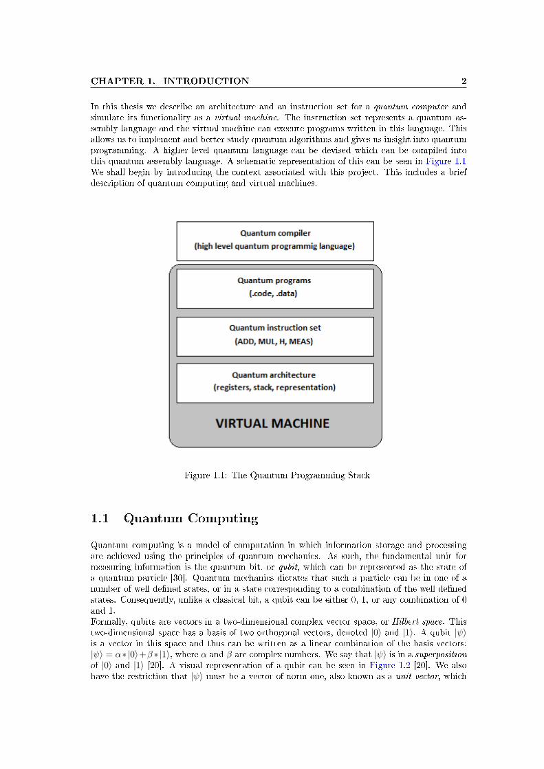
In this thesis we describe an architecture and an instruction set for a quantum computer andsimulate its functionality as a virtual machine. The instruction set represents a quantum as-sembly language and the virtual machine can execute programs written in this language. Thisallows us to implement and better study quantum algorithms and gives us insight into quantumprogramming. A higher level quantum language can be devised which can be compiled intothis quantum assembly language. A schematic representation of this can be seen in Figure 1.1We shall begin by introducing the context associated with this project. This includes a briefdescription of quantum computing and virtual machines.
Figure 1.1: The Quantum Programming Stack
1.1 Quantum Computing
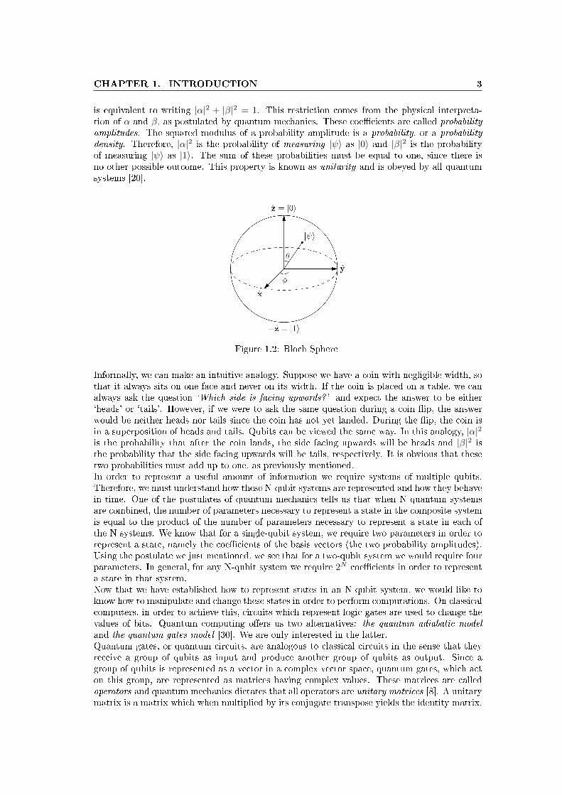
Quantum computing is a model of computation in which information storage and processingare achieved using the principles of quantum mechanics. As such, the fundamental unit formeasuring information is the quantum bit, or qubit, which can be represented as the state ofa quantum particle [30]. Quantum mechanics dictates that such a particle can be in one of anumber of well dened states, or in a state corresponding to a combination of the well denedstates. Consequently, unlike a classical bit, a qubit can be either 0, 1, or any combination of 0and 1.Formally, qubits are vectors in a two-dimensional complex vector space, or Hilbert space. Thistwo-dimensional space has a basis of two orthogonal vectors, denoted |0〉 and |1〉. A qubit |ψ〉is a vector in this space and thus can be written as a linear combination of the basis vectors:|ψ〉 = α∗|0〉+β ∗|1〉, where α and β are complex numbers. We say that |ψ〉 is in a superpositionof |0〉 and |1〉 [20]. A visual representation of a qubit can be seen in Figure 1.2 [20]. We alsohave the restriction that |ψ〉 must be a vector of norm one, also known as a unit vector, which
CHAPTER 1. INTRODUCTION 3
is equivalent to writing |α|2 + |β|2 = 1. This restriction comes from the physical interpreta-tion of α and β, as postulated by quantum mechanics. These coecients are called probabilityamplitudes. The squared modulus of a probability amplitude is a probability, or a probabilitydensity. Therefore, |α|2 is the probability of measuring |ψ〉 as |0〉 and |β|2 is the probabilityof measuring |ψ〉 as |1〉. The sum of these probabilities must be equal to one, since there isno other possible outcome. This property is known as unitarity and is obeyed by all quantumsystems [20].
Figure 1.2: Bloch Sphere
Informally, we can make an intuitive analogy. Suppose we have a coin with negligible width, sothat it always sits on one face and never on its width. If the coin is placed on a table, we canalways ask the question `Which side is facing upwards?' and expect the answer to be either`heads' or `tails'. However, if we were to ask the same question during a coin ip, the answerwould be neither heads nor tails since the coin has not yet landed. During the ip, the coin isin a superposition of heads and tails. Qubits can be viewed the same way. In this analogy, |α|2is the probability that after the coin lands, the side facing upwards will be heads and |β|2 isthe probability that the side facing upwards will be tails, respectively. It is obvious that thesetwo probabilities must add up to one, as previously mentioned.In order to represent a useful amount of information we require systems of multiple qubits.Therefore, we must understand how these N-qubit systems are represented and how they behavein time. One of the postulates of quantum mechanics tells us that when N quantum systemsare combined, the number of parameters necessary to represent a state in the composite systemis equal to the product of the number of parameters necessary to represent a state in each ofthe N systems. We know that for a single-qubit system, we require two parameters in order torepresent a state, namely the coecients of the basis vectors (the two probability amplitudes).Using the postulate we just mentioned, we see that for a two-qubit system we would require fourparameters. In general, for any N-qubit system we require 2N coecients in order to representa state in that system.Now that we have established how to represent states in an N-qubit system, we would like toknow how to manipulate and change these states in order to perform computations. On classicalcomputers, in order to achieve this, circuits which represent logic gates are used to change thevalues of bits. Quantum computing oers us two alternatives: the quantum adiabatic modeland the quantum gates model [30]. We are only interested in the latter.Quantum gates, or quantum circuits, are analogous to classical circuits in the sense that theyreceive a group of qubits as input and produce another group of qubits as output. Since agroup of qubits is represented as a vector in a complex vector space, quantum gates, which acton this group, are represented as matrices having complex values. These matrices are calledoperators and quantum mechanics dictates that all operators are unitary matrices [8]. A unitarymatrix is a matrix which when multiplied by its conjugate transpose yields the identity matrix.
CHAPTER 1. INTRODUCTION 4
The restriction that quantum gates can only be represented as unitary matrices has importantconsequences for quantum computing. First of all, applying a unitary operator to a vector willnot change its norm. Since we are working with unit vectors, unitarity is preserved. Secondly,unitary matrices are always invertible [8]. This leads to the interesting fact that all quantumoperations are reversible which means that any input, of a set of quantum operations, can beobtained from the output by applying the reverse operations on the output. This is a majordierence from classical gates which are not always reversible. A good example is the logicalAND gate where, if we obtain an output of 0, we only know that one of the input bits is 0, butwe do not know which one and therefore we cannot reconstitute the input from the output.In the quantum gates model, a quantum computer is a device which represents information asqubits and performs computations using quantum gates as previously described [30]. One ofthe objectives of our project is to simulate such a quantum computer. To that end, in the nextsection we introduce the context of virtual machines.
1.2 Virtual Machines
A virtual machine, is a software program that simulates a functioning computer architecture.It is an abstraction of a real or hypothetical hardware model. The original denition of a VMgiven by Popek and Goldberg is an ecient, isolated duplicate of a real machine [23]. ModernVMs may have no correspondence to an actual physical machine, as is the case with our project[26].In order to simulate a computing machine we need to dene an architecture for that machineand a low-level instruction set associated with the architecture. The VM will execute theseinstructions thus simulating the execution of the computing machine. We can thus view theVM as an interpreter, a program which takes as input instructions written in a well-denedlanguage and executes these instructions. However, it should be made clear that VMs and in-terpreters are not equivalent. Interpreters impose no restrictions regarding which programminglanguages can be interpreted. VMs, on the other hand, require that the interpreted languagebe a low-level instruction set corresponding to a certain architecture.In the context of our application, we are interested in a process virtual machine. A process VMsupports a single process and is implemented using an interpreter. The most popular VM of thistype is the Java Virtual Machine. The JVM executes Java bytecode, produced by compilingJava source les [27]. The main advantage of this approach is portability: for a Java source lethe same bytecode is produced, regardless of the host platform architecture, since the VM willinterpret the bytecode. The idea is illustrated by the Sun Microsystems slogan write once, runanywhere.Since the hardware which is simulated is not necessarily real, the architecture specication canbe reasonably abstract. This means that there is only a certain set of architectural elementswhich need to be specied: number of registers, register sizes, number representation, memoryrepresentation, existence of a stack etc. These will be discussed in detail in the following sec-tions for our specic implementation.
1.3 Project Objectives and Motivation
The project's main objectives can be summarized as follows:
• Design a quantum computer architecture which is consistent with the quantum computingmodel. This computer must be quantum Turing complete, i.e. equivalent to a quantumTuring machine [30]. Furthermore, the architecture will make no assumptions regarding
CHAPTER 1. INTRODUCTION 5
the physical implementation of each hardware component and will work with abstractionsof such components.
• Design a set of low-level instructions for the computer architecture. The set of instructionswill represent a quantum assembly language which can be used in order to write andexecute programs on the quantum computer. The architecture and instruction set willfollow a Reduced Instruction Set Computing (RISC) design strategy.
• Implement a VM which simulates the chosen architecture and interprets the instructionsfrom the quantum assembly language. The virtual machine will be the abstraction ofthe quantum computer. It will be capable of executing programs written in the quantumassembly language and provide information on its internal state (registers content, usedmemory etc).
The primary motivation for this project is the better understanding of quantum programmingand the advantages quantum computing oers over classical computing. The VM will be testedwith various programs. Some of these programs will be written manually, while others will begenerated by a quantum compiler designed to generate code in the quantum assembly languagethat we have designed. We aim to show how the number of instructions required to solve aset of problems on a quantum computer is signicantly smaller than on a classical computer.This is a direct result of the fact that the quantum algorithms used to solve these problemsare quadratically or even exponentially faster than their classical counterparts. We also wishto explore the implementation of these algorithms in the quantum assembly language, thusgaining insight into quantum programming. The proposed quantum architecture may serve asa template for an actual physical implementation. Such an implementation would be able toexecute the quantum instruction set directly thus eliminating the overhead associated with asimulation on a classical computer.
Chapter 2
Quantum Computation
In this chapter we focus on how quantum computations are performed, emphasizing the quan-tum gates model, quantum operations and the model we have used in our VM. We start bydescribing a quantum Turing machine and then proceed to the equivalent quantum gates model.We then describe the most important quantum operations and discuss the possibility of univer-sal quantum gates. Finally, the model we have adopted is presented, using all of the previouslymentioned topics.
2.1 Model of computation
2.1.1 Church-Turing-Deutsch principle
A model of computation is a mathematical formalism for an abstract machine which performscomputations. Many models of computation exist, such as lambda calculus, nite state ma-chines, recursive functions, but the rst and most popular one is the Turing machine. AlanTuring came up with this model in an attempt to formalize how we perform computations, thusgiving rise to the notion of a computer [28]. He and others then tried to determine what canand cannot be computed. In this context, to compute something means to perform some taskby algorithmic means. This led to the Church-Turing thesis which states that any algorithmicprocess can be simulated using a Turing machine [20]. This basically establishes the Turingmachine as the most powerful model of computation, in the sense that, so far, no other modelis known which can compute something that the Turing machine cannot.While the Church-Turing thesis tells us what Turing machines can compute, it does not tell ushow ecient they are at performing such computations. The concepts of ecient and ine-cient algorithms are formally dened by computational complexity theory. Strictly speaking, anecient algorithm is one which runs in polynomial time with respect to the size of the problem.An inecient algorithm runs in superpolynomial (usually exponential) time [20]. Initially, itwas observed that any problem which could be solved eciently by any model of computation,could also be solved eciently by a Turing machine. This led to a new version of the Church-Turing thesis called the strong Church-Turing thesis which states that any algorithmic processcan be simulated eciently using a Turing machine [20]. The only dierence is that the wordeciently has been added. The strong Church-Turing thesis was challenged by the emergenceof randomized algorithms. Randomized algorithms, while not exact, are useful for testing theprimality of natural numbers. They have the advantage of being ecient and there are noknown equivalent, ecient, deterministic algorithms. This led to the development of anothermodel of computation known as a probabilistic Turing machine. This model led to a changeof the strong Church-Turing thesis: any algorithmic process can be simulated eciently using
6
CHAPTER 2. QUANTUM COMPUTATION 7
a probabilistic Turing machine [20].The next change came in trying to determine if a Turing machine can eciently simulate anarbitrary physical system. As previously mentioned, Richard Feynman came to the conclusionthat nature cannot be simulated by classical means and an eective simulation would have tobe based on quantum mechanics. David Deutsch arrived at a similar conclusion in 1985 [9].He formulated the Church-Turing-Deutsch principle which states that a universal computingdevice can simulate every physical process. He proposed a model for a quantum Turing machineand suggested that a quantum computer based on this model would obey the Church-Turing-Deutsch principle, assuming quantum mechanics can completely describe every physical process.He also showed that a quantum Turing machine could eciently solve problems that have noecient solution on a classical computer or even a probabilistic one [9].
2.1.2 Quantum gates and circuits
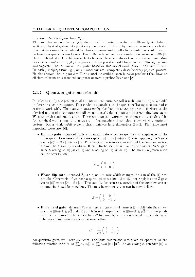
In order to study the properties of a quantum computer we will use the quantum gates modelto describe such a computer. This model is equivalent to the quantum Turing machine and iseasier to work with. The quantum gates model also has the advantage that it is closer to thephysical notion of a computer and allows us to easily dene quantum programming languages.We start with single-qubit gates. These are quantum gates which operate on a single qubit.As explained earlier, quantum gates are in fact matrices of complex values which operate onvectors. For a single-qubit system, these matrices have dimensions 2 × 2. The three mostimportant gates are [20]:
• Bit ip gate - denoted X, is a quantum gate which swaps the two amplitudes of theinput qubit. Concretely, if we have a qubit |ψ〉 = α∗|0〉+β ∗|1〉, then applying the X gateyields |ψ〉′ = β ∗ |0〉+ α ∗ |1〉. This can also be seen as a rotation of the complex vector,around the X axis by π radians. It can also be seen as similar to the classical NOT gatesince X acting on |0〉 yields |1〉 and X acting on |1〉 yields |0〉. The matrix representationcan be seen bellow:
X =
(0 11 0
)• Phase ip gate - denoted Z, is a quantum gate which changes the sign of the |1〉 am-plitude. Concretely, if we have a qubit |ψ〉 = α ∗ |0〉 + β ∗ |1〉, then applying the Z gateyields |ψ〉′ = α ∗ |0〉 − β ∗ |1〉. This can also be seen as a rotation of the complex vector,around the Z axis by π radians. The matrix representation can be seen bellow:
Z =
(1 00 −1
)• Hadamard gate - denoted H, is a quantum gate which turns a |0〉 qubit into the super-position (|0〉+|1〉)/
√2 and a |1〉 qubit into the superposition (|0〉−|1〉)/
√2. It corresponds
to a rotation around the Y axis by π/2 followed by a rotation around the X axis by π.The matrix representation can be seen bellow:
H =1√2
(1 11 −1
)All quantum gates are linear operators. Formally, this means that given an operator M thefollowing relation is true: M(
∑i αi |vi〉) =
∑i αiM |vi〉 [20]. As an example, consider |ψ〉 =
CHAPTER 2. QUANTUM COMPUTATION 8
α ∗ |0〉 + β ∗ |1〉. If we wish to apply the Hadamard gate there are two possible approaches.First, we could use the matrix representation and multiply the H matrix with the |ψ〉 vector:
1√2
(1 11 −1
)(αβ
)=
1√2
(α+ βα− β
)The second approach relies on the linearity property:
H |ψ〉 = α ∗H |0〉+ β ∗H |1〉 (2.1)
Since we know that:
H |0〉 =|0〉+ |1〉√
2H |1〉 =
|0〉 − |1〉√2
(2.2)
We will obtain:
H |ψ〉 = α|0〉+ |1〉√
2+ β|0〉 − |1〉√
2(2.3)
H |ψ〉 =α+ β√
2|0〉+
α− β√2|1〉 (2.4)
The same result was obtained with the matrix representation.It will be convenient to adopt a circuit representation of these gates. This representation willhelp us explain certain algorithms in terms of quantum circuits. The circuit representations ofgates X, Z and H is given in Figure 2.1 [20].
Figure 2.1: Quantum gates as circuits
Other single-qubit gates are: the Y gate, which applies a rotation by π around the Y axis, thephase shift gate which maps the |1〉 vector to eiθ |1〉, for some angle θ and leaves the |0〉 vectorunchanged.Apart from the single-qubit gates, we will also be using some two-qubit gates. As mentionedpreviously, a two-qubit system is described by four complex amplitudes. A general representa-tion of a two-qubit state is: |ψ〉 = α0 |00〉 + α1 |01〉 + α2 |10〉 + α3 |11〉. Since we have vectorsof four components, our matrix operators will have dimensions 4× 4. The two-qubit gates wewill be using are:
• SWAP gate - a gate which receives two qubits as input and interchanges their values.The matrix representation can be seen bellow:
SWAP =
1 0 0 00 0 1 00 1 0 00 0 0 1
CHAPTER 2. QUANTUM COMPUTATION 9
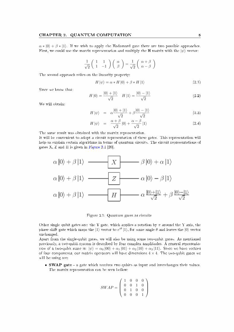
• CNOT gate - the controlled NOT gate leaves the rst qubit unchanged and ips thesecond one if the rst qubit is |1〉. The matrix representation can be seen bellow:
CNOT =
1 0 0 00 1 0 00 0 0 10 0 1 0
The CNOT gate can be viewed as the quantum analog to the classical XOR gate. The secondoutput qubit will be the two input qubits XOR-ed. To write this, we will use the followingnotation |ab〉 is equivalent to |a, b〉. Then, for input |a, b〉 to the CNOT gate, with |a〉 as thecontrol qubit, the output will be |a, a⊕ b〉.A circuit representation of these two gates is given in Figure 2.2 [29].
Figure 2.2: CNOT and SWAP gates
A question we may pose is How do two single-qubit gates translate to a two-qubit gate?.Specically, if we have an input state consisting of two qubits |x, y〉 and we apply the single-qubit operator A to x and the single-qubit operator B to y, we wish to determine the resultingtwo-qubit operator which was applied to the initial state. The answer is given by the tensorproduct, denoted ⊗. Consider
A =
(a11 a12a21 a22
)B =
(b11 b12b21 b22
)Then the resulting two-qubit operator is:
A⊗B =
(a11 a12a21 a22
)⊗(b11 b12b21 b22
)=
a11b11 a11b12 a12b11 a12b12a11b21 a11b22 a12b21 a12b22a21b11 a21b12 a22b11 a22b12a21b21 a21b22 a22b21 a22b22
Since quantum gates are unitary operators, if we wish to implement a classical gate or functionas a quantum gate we must make sure that the resulting operator is unitary and consequentlyinvertible. An example is the CNOT gate itself. As mentioned, the CNOT gate is the quantumanalog to the classical XOR gate, however the classical XOR gate has two inputs and oneoutput. In the quantum case we are forced to have two outputs since the dimensions of theoutput vector must match that of the input vector. Furthermore, the extra output qubit cannotbe an arbitrary value, it must be carefully selected so as to ensure that the operator is unitary.This means that if we wish to construct a quantum operator corresponding to some classicalnon-invertible function, we have to add extra qubits to ensure that dimensions match and theoperator is invertible. These extra qubits are refered to as junk qubits. This could presenta problem, since the junk qubits may aect our computations through various superpositions[29]. It is thus desirable to eliminate the junk qubits.
CHAPTER 2. QUANTUM COMPUTATION 10
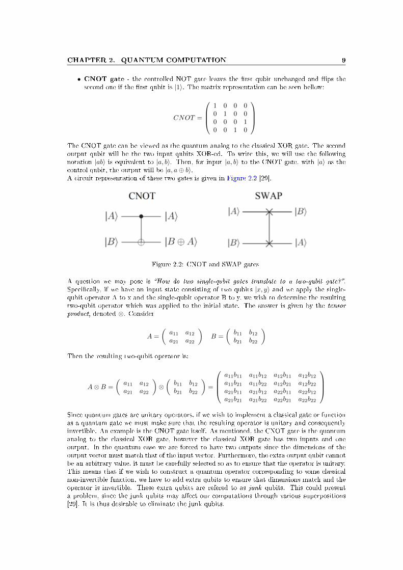
We would like to obtain a black-box model for any unitary operator Uf , representing thequantum analog to some classical function f . This black box model would take the input |x, y〉and map it to |x, y ⊕ f(x)〉. Assuming we are able to construct a unitary operator Uf forsome classical function f , which outputs |f(x)〉 and some junk qubits, we can use the circuit inFigure 2.3 [29] to remove the junk qubits. This circuit uses the CNOT gate and relies on the factthat since Uf is unitary we can obtain its inverse U−1f and use it to remove the unwanted junk.If we ignore the zeros, we have obtained our black-box model. From now on, for any classicalfunction f , we shall refer to this black-box model as Uf . Assuming we are only interested inf(x) we can set y to all zeros.
Figure 2.3: Circuit to eliminate junk qubits
2.2 Eciency of quantum computers
2.2.1 Quantum parallelism
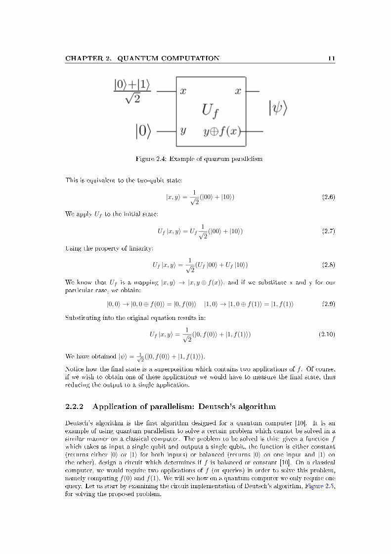
The main reason quantum computers can solve certain problems more eciently than classicalcomputers is quantum parallelism. Roughly speaking, quantum parallelism allows quantumcomputers to evaluate a function f(x) for many dierent values of x simultaneously. Thisis possible because of two things: superposition, which allows a quantum state to exist as acombination of multiple states, and linearity of quantum operators [20]. Care must be takenwhen discussing quantum parallelism so as to not misunderstand the concept. While it is truethat it allows for the simultaneous evaluation of a function for multiple inputs, it does not meanthat all of these function applications are directly usable. These applications will be containedin a superposition, which upon measurement, will collapse into a single state, corresponding toa certain application.We shall consider the example from Figure 2.4 [20] to properly understand quantum parallelism.Here we have a quantum operator Uf associated to a certain classical function f . We are usingthe black-box model, so there will be two inputs denoted by the state |x, y〉 and two outputsdenoted by the state |x, y ⊕ f(x)〉. In this example, we are assuming x and y to be singlequbits, thus Uf is a two-qubit operator. We denote the output state as |ψ〉. We wish to seewhat happens when the input x is a superposition, x = (|0〉+ |1〉)/
√2. We will set y to |0〉 so
as to obtain f(x) as the second output qubit. We proceed with a step-by-step analysis of theevolution of the initial state. Our input qubits are:
x =|0〉+ |1〉√
2y = |0〉 (2.5)
CHAPTER 2. QUANTUM COMPUTATION 11
Figure 2.4: Example of quantum parallelism
This is equivalent to the two-qubit state:
|x, y〉 =1√2
(|00〉+ |10〉) (2.6)
We apply Uf to the initial state:
Uf |x, y〉 = Uf1√2
(|00〉+ |10〉) (2.7)
Using the property of liniarity:
Uf |x, y〉 =1√2
(Uf |00〉+ Uf |10〉) (2.8)
We know that Uf is a mapping |x, y〉 → |x, y ⊕ f(x)〉, and if we substitute x and y for ourparticular case, we obtain:
|0, 0〉 → |0, 0⊕ f(0)〉 = |0, f(0)〉 |1, 0〉 → |1, 0⊕ f(1)〉 = |1, f(1)〉 (2.9)
Substituting into the original equation results in:
Uf |x, y〉 =1√2
(|0, f(0)〉+ |1, f(1)〉) (2.10)
We have obtained |ψ〉 = 1√2(|0, f(0)〉+ |1, f(1)〉).
Notice how the nal state is a superposition which contains two applications of f . Of course,if we wish to obtain one of these applications we would have to measure the nal state, thusreducing the output to a single application.
2.2.2 Application of parallelism: Deutsch's algorithm
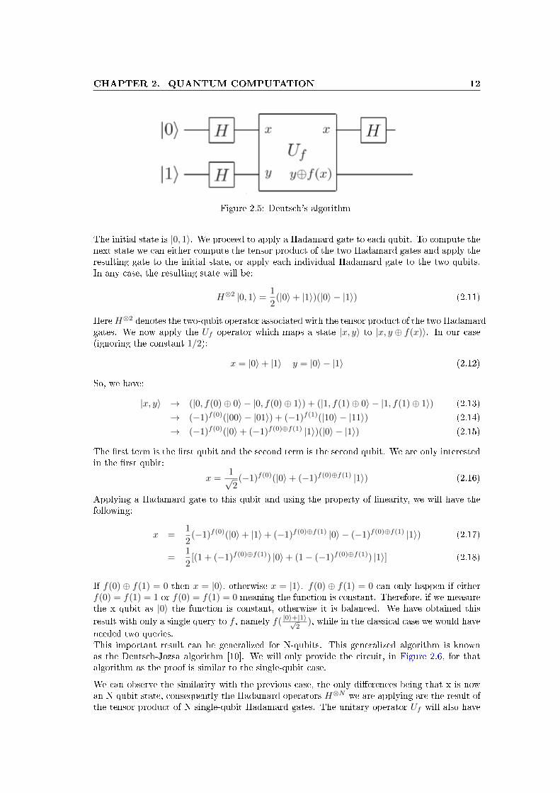
Deutsch's algorithm is the rst algorithm designed for a quantum computer [10]. It is anexample of using quantum parallelism to solve a certain problem which cannot be solved in asimilar manner on a classical computer. The problem to be solved is this: given a function fwhich takes as input a single qubit and outputs a single qubit, the function is either constant(returns either |0〉 or |1〉 for both inputs) or balanced (returns |0〉 on one input and |1〉 onthe other), design a circuit which determines if f is balanced or constant [10]. On a classicalcomputer, we would require two applications of f (or queries) in order to solve this problem,namely computing f(0) and f(1). We will see how on a quantum computer we only require onequery. Let us start by examining the circuit implementation of Deutsch's algorithm, Figure 2.5,for solving the proposed problem.
CHAPTER 2. QUANTUM COMPUTATION 12
Figure 2.5: Deutsch's algorithm
The initial state is |0, 1〉. We proceed to apply a Hadamard gate to each qubit. To compute thenext state we can either compute the tensor product of the two Hadamard gates and apply theresulting gate to the initial state, or apply each individual Hadamard gate to the two qubits.In any case, the resulting state will be:
H⊗2 |0, 1〉 =1
2(|0〉+ |1〉)(|0〉 − |1〉) (2.11)
HereH⊗2 denotes the two-qubit operator associated with the tensor product of the two Hadamardgates. We now apply the Uf operator which maps a state |x, y〉 to |x, y ⊕ f(x)〉. In our case(ignoring the constant 1/2):
x = |0〉+ |1〉 y = |0〉 − |1〉 (2.12)
So, we have:
|x, y〉 → (|0, f(0)⊕ 0〉 − |0, f(0)⊕ 1〉) + (|1, f(1)⊕ 0〉 − |1, f(1)⊕ 1〉) (2.13)
→ (−1)f(0)(|00〉 − |01〉) + (−1)f(1)(|10〉 − |11〉) (2.14)
→ (−1)f(0)(|0〉+ (−1)f(0)⊕f(1) |1〉)(|0〉 − |1〉) (2.15)
The rst term is the rst qubit and the second term is the second qubit. We are only interestedin the rst qubit:
x =1√2
(−1)f(0)(|0〉+ (−1)f(0)⊕f(1) |1〉) (2.16)
Applying a Hadamard gate to this qubit and using the property of linearity, we will have thefollowing:
x =1
2(−1)f(0)(|0〉+ |1〉+ (−1)f(0)⊕f(1) |0〉 − (−1)f(0)⊕f(1) |1〉) (2.17)
=1
2[(1 + (−1)f(0)⊕f(1)) |0〉+ (1− (−1)f(0)⊕f(1)) |1〉] (2.18)
If f(0) ⊕ f(1) = 0 then x = |0〉, otherwise x = |1〉. f(0) ⊕ f(1) = 0 can only happen if eitherf(0) = f(1) = 1 or f(0) = f(1) = 0 meaning the function is constant. Therefore, if we measurethe x qubit as |0〉 the function is constant, otherwise it is balanced. We have obtained this
result with only a single query to f , namely f( |0〉+|1〉√2
), while in the classical case we would have
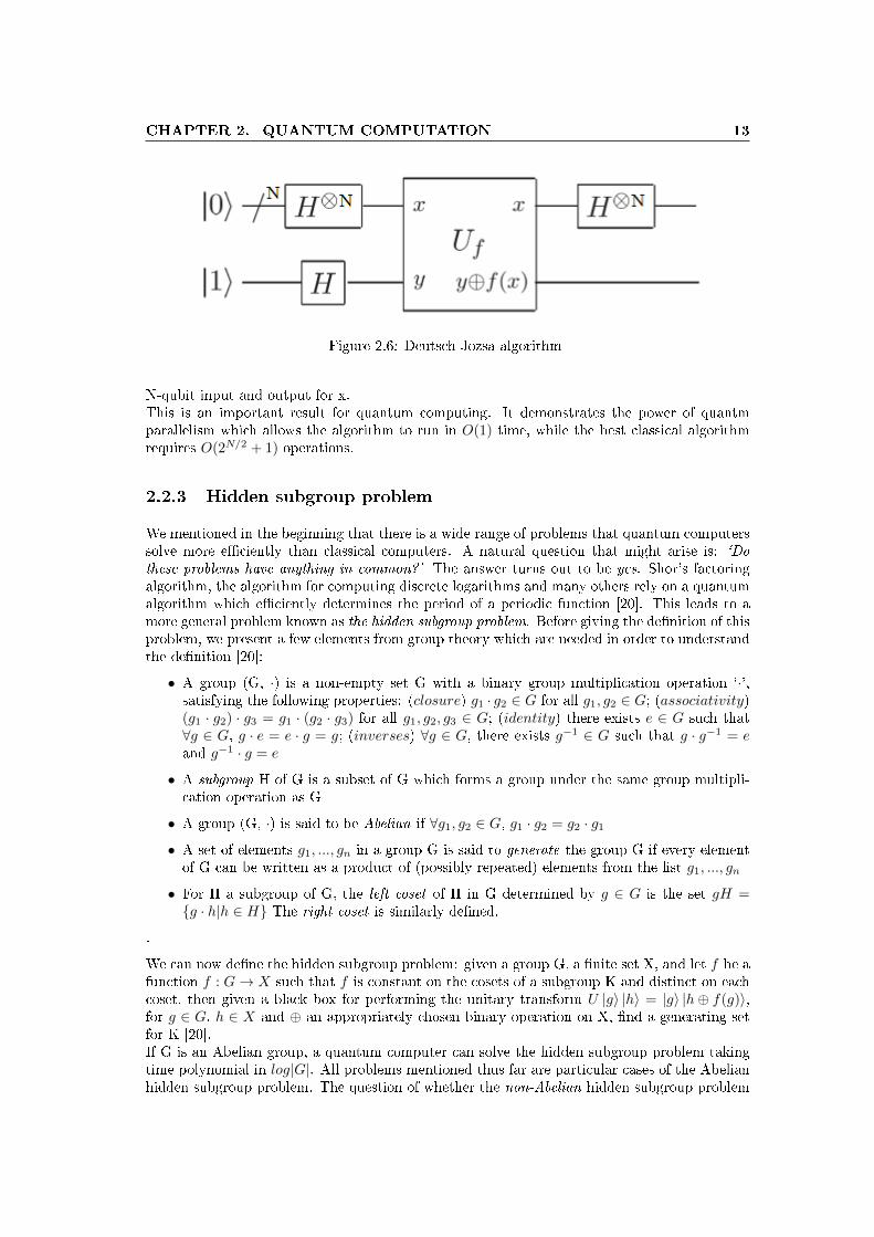
needed two queries.This important result can be generalized for N-qubits. This generalized algorithm is knownas the Deutsch-Jozsa algorithm [10]. We will only provide the circuit, in Figure 2.6, for thatalgorithm as the proof is similar to the single-qubit case.
We can observe the similarity with the previous case, the only dierences being that x is nowan N-qubit state, consequently the Hadamard operators H⊗N we are applying are the result ofthe tensor product of N single-qubit Hadamard gates. The unitary operator Uf will also have
CHAPTER 2. QUANTUM COMPUTATION 13
Figure 2.6: Deutsch-Jozsa algorithm
N-qubit input and output for x.This is an important result for quantum computing. It demonstrates the power of quantmparallelism which allows the algorithm to run in O(1) time, while the best classical algorithmrequires O(2N/2 + 1) operations.
2.2.3 Hidden subgroup problem
We mentioned in the beginning that there is a wide range of problems that quantum computerssolve more eciently than classical computers. A natural question that might arise is: `Dothese problems have anything in common?' The answer turns out to be yes. Shor's factoringalgorithm, the algorithm for computing discrete logarithms and many others rely on a quantumalgorithm which eciently determines the period of a periodic function [20]. This leads to amore general problem known as the hidden subgroup problem. Before giving the denition of thisproblem, we present a few elements from group theory which are needed in order to understandthe denition [20]:
• A group (G, ·) is a non-empty set G with a binary group multiplication operation `·',satisfying the following properties: (closure) g1 · g2 ∈ G for all g1, g2 ∈ G; (associativity)(g1 · g2) · g3 = g1 · (g2 · g3) for all g1, g2, g3 ∈ G; (identity) there exists e ∈ G such that∀g ∈ G, g · e = e · g = g; (inverses) ∀g ∈ G, there exists g−1 ∈ G such that g · g−1 = eand g−1 · g = e
• A subgroup H of G is a subset of G which forms a group under the same group multipli-cation operation as G
• A group (G, ·) is said to be Abelian if ∀g1, g2 ∈ G, g1 · g2 = g2 · g1• A set of elements g1, ..., gn in a group G is said to generate the group G if every elementof G can be written as a product of (possibly repeated) elements from the list g1, ..., gn
• For H a subgroup of G, the left coset of H in G determined by g ∈ G is the set gH =g · h|h ∈ H The right coset is similarly dened.
.
We can now dene the hidden subgroup problem: given a group G, a nite set X, and let f be afunction f : G→ X such that f is constant on the cosets of a subgroup K and distinct on eachcoset, then given a black box for performing the unitary transform U |g〉 |h〉 = |g〉 |h⊕ f(g)〉,for g ∈ G, h ∈ X and ⊕ an appropriately chosen binary operation on X, nd a generating setfor K [20].If G is an Abelian group, a quantum computer can solve the hidden subgroup problem takingtime polynomial in log|G|. All problems mentioned thus far are particular cases of the Abelianhidden subgroup problem. The question of whether the non-Abelian hidden subgroup problem
CHAPTER 2. QUANTUM COMPUTATION 14
can also be solved eciently remains an open question. It is also currently unknown if quantumcomputers can be used to eciently solve NP-complete problems. They can, however, providea speed-up in solving such problems. In general, these are search problems solved by brute-force algorithms having O(2n) temporal complexity. A quantum search algorithm by Groverprovides a quadratic speedup over the traditional, classical search for an element in an unsorteddatabase. Using this algorithm for NP-complete problems yields a complexity of O(2n/2) [7].
2.2.4 Quantum entanglement
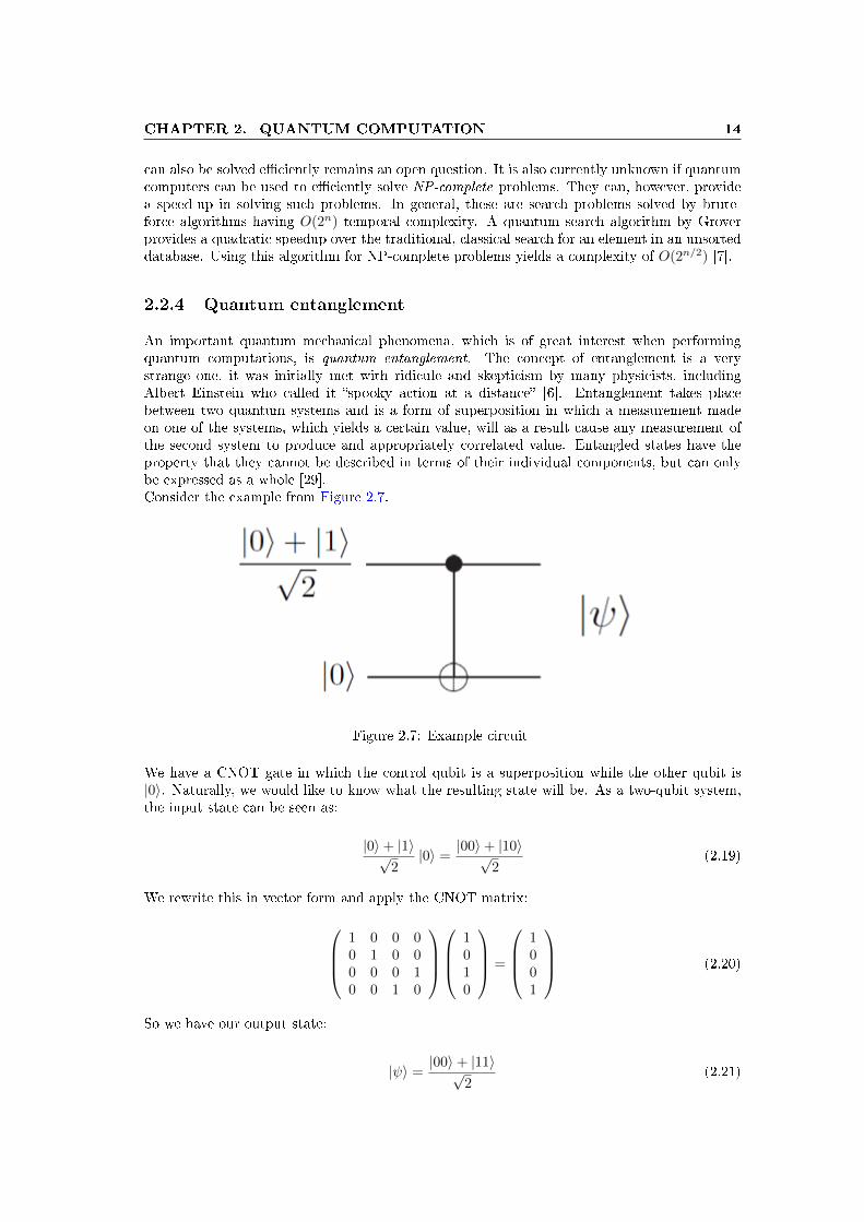
An important quantum mechanical phenomena, which is of great interest when performingquantum computations, is quantum entanglement. The concept of entanglement is a verystrange one, it was initially met with ridicule and skepticism by many physicists, includingAlbert Einstein who called it spooky action at a distance [6]. Entanglement takes placebetween two quantum systems and is a form of superposition in which a measurement madeon one of the systems, which yields a certain value, will as a result cause any measurement ofthe second system to produce and appropriately correlated value. Entangled states have theproperty that they cannot be described in terms of their individual components, but can onlybe expressed as a whole [29].Consider the example from Figure 2.7.
Figure 2.7: Example circuit
We have a CNOT gate in which the control qubit is a superposition while the other qubit is|0〉. Naturally, we would like to know what the resulting state will be. As a two-qubit system,the input state can be seen as:
|0〉+ |1〉√2|0〉 =
|00〉+ |10〉√2
(2.19)
We rewrite this in vector form and apply the CNOT matrix:
1 0 0 00 1 0 00 0 0 10 0 1 0
1010
=
1001
(2.20)
So we have our output state:
|ψ〉 =|00〉+ |11〉√
2(2.21)

CHAPTER 2. QUANTUM COMPUTATION 15
This state, has the interesting property that it cannot be expressed in terms of two qubits. Thiscan be proven by reductio ad absurdum. Assume we can write |ψ〉 in terms of two qubits. Thatwould mean that:
|ψ〉 = (α1 |0〉+ β1 |1〉)(α2 |0〉+ β2 |1〉) =|00〉+ |11〉√
2(2.22)
Which is equivalent to the four equations:
α1α2 = 1 (2.23)
α1β2 = 0 (2.24)
β1α2 = 0 (2.25)
β1β2 = 1 (2.26)
Which is obviously a contradiction. Therefore, our initial assumption is false.The state |ψ〉 is known as a Bell state and there are three others [29]:∣∣Φ+
⟩=|00〉+ |11〉√
2∣∣Φ−⟩ =|00〉 − |11〉√
2∣∣Ψ+⟩
=|01〉+ |10〉√
2∣∣Ψ−⟩ =|01〉 − |10〉√
2
The signicance of quantum entanglement for our application will be discussed when we talkabout quantum memory.
2.3 Universal quantum computer
2.3.1 Universal gate set
A universal quantum computer, or UQC, is a computer which is equivalent to a quantumTuring machine. We mentioned that the quantum gates model is equivalent to a quantumTuring machine, therefore we can use quantum gates to construct a UQC [20]. However, we arefaced with the following question: Which gates do we use in implementing such a computer?Obviously, there are innitely many quantum operators, yet we must use a nite set of theseoperators to implement our UQC. In classical computing, we have the concept of universalgates, logical gates which can be used to implement any classical circuit. A prime example isthe classical NAND gate. Another example is the Tooli gate, also known as the CCNOT gate.This gate is of interest to us because it is a reversible gate, hence it can be implemented as aquantum operator. This proves that the family of quantum circuits includes that of classicalcircuits [20].The concept of universal quantum gates diers from that of classical universal gates. A setof gates is said to be universal for quantum computation if any unitary operation may beapproximated to arbitrary accuracy by a quantum circuit involving only those gates. A set ofquantum universal gates is, for example: Hadamard, CNOT, phase gate (denoted S, not to beconfused with the phase ip gate, Z) and the T gate [20]. The last two gates are representedbellow:
S =
(1 00 i
)T =
(1 00 eiπ/4
)
CHAPTER 2. QUANTUM COMPUTATION 16
We will not prove why this set of gates is universal, however the general idea is the following:it can be shown that any N-qubit operator can be expressed exactly as a product of two-levelunitary matrices. Two-level unitary matrices are matrices which act non-trivially on two orfewer vector components. It can also be shown, that any two-level unitary matrix can be con-structed exactly using single-qubit and CNOT gates [20]. We have thus reduced the problem toexpressing any single-qubit operator as a combination of a specic set of single-qubit operators,which will represent the universal set. This cannot be done exactly, however it is possible toapproximate any single-qubit gate to arbitrary precision using as many gates from the universalset as needed. Unfortunately, some N-qubit operators require exponentially many gates in orderto approximate, but that will not be the case for most applications. Approximating single-qubitoperators does not require as many gates. A theorem, known as the Solovay-Kitaev theorem,states that the number of gates required in order to approximate a given single-qubit operatorup to precision ε is of the order O(logc(1/ε)), where 1 < c < 2 [20].Our model will include this universal gate set and a few other gates to facilitate a wider rangeof possibilities for representing unitary operators.
2.3.2 Physical implementation
Currently, the physical implementation of a quantum computer is generally considered a chal-lenging problem. Most of the existing quantum computers are based on the adiabatic modelrather than the quantum gates model [13]. Such quantum computers have been constructed bythe D-Wave Systems corporation [5]. However, these computers are not equivalent to the UQCand the set of operations they can perform is limited.The most advanced quantum computer based on the quantum gates model to date was able tofactor the number 15 into 3 and 5 [18]. The reason for this is that quantum gates are very hardto construct physically. There are many problems associated with creating and maintainingpure quantum states [30, 20]:
• The main problem is quantum decoherence. Coherence is a correlation established betweenquantum states which are in superposition. If these quantum states interact with thesurrounding environment in such a way that the correlation is lost, we say that thequantum states have decohered. The problem of quantum decoherence is that it is verydicult to maintain pure quantum states (superpositions) isolated from the environment.
• The problem of storing quantum information. If we store a value in a quantum register,we expect the register to maintain and not alter that value if the register is not used. Asan example, if we store |00000000〉 in an 8-qubit register and after some time the value hasspontaneously changed to |00000001〉 (becuase of some external factor, such as thermalnoise for example), then the register is not storing information correctly.
• The problem of imperfect quantum gates. Quantum gates may contain or develop imper-fections leading to incorrect operators being used. This may be very dicult to detect,especially when working with pure quantum states. The imperfections could also lead todecoherence of quantum states.
• The problem of incorrect measurement. Since quantum operations must be unitary andreversible, they are isolated from any classical operations. The interface between quantumand classical systems is given by measurements, which collapse quantum states and oerclassical information pertaining to the quantum system. Since pure quantum states willrandomly collapse to one of the basis states, this randomness makes it dicult to detecterrors in measurement.
Of the attempts made to construct gate-based quantum computers, the following models forphysical systems have been explored [20]:
• Harmonic oscillator quantum computer
CHAPTER 2. QUANTUM COMPUTATION 17
• Optical photon quantum computer
• Optical cavity quantum electrodynamics
• Ion traps
• Nuclear magnetic resonance
2.3.3 Virtual implementation
Considering the aforementioned problems with a physical realization of a quantum computer,we explore the idea of a virtual implementation, or a simulation of a quantum computer by aclassical computer. We recognize that the physical problems such as decoherence, noise andimperfections do not arise in a virtual implementation. However, there are several problemswith this approach as well. We proceed to name a few of these problems:
• The main problem is that simulating a quantum computer on a classical machine doesnot allow us to exploit the benets of quantum parallelism. Many aspects associatedwith the quantum computer require exponential time and space to simulate on a classicalcomputer. For example, storing an N-qubit register requires storing 2N complex numbers,representing the amplitudes of the N-qubit state [20].
• Precision in representation is also a problem. It is obvious that a computer has a lim-ited precision in representing real numbers. Consequently, quantum states can only berepresented to a certain level of approximation.
• Quantum mechanics works with true random events. A classical computer, however, is adeterministic machine that works with pseudo-random numbers. This again means thatwe are only working with an approximate model.
In spite of these diculties, a virtual implementation is worth pursuing as it gives us insightinto quantum programming and can provide a template for a physical implementation.As with the physical case, there are several possible models which can be explored when imple-menting a virtual quantum computer:
• Simulating a quantum Turing machine. This is perhaps the simplest approach, but alsothe most dicult to work with and the least closer to an actual physical device.
• Simulating the physical system that implements a quantum computer. This means simu-lating one of the previously mentioned physical models for constructing a quantum com-puter. This approach is not advantageous because simulating a physical model is a com-putationally intensive task even for a quantum computer with few and small registers.
• Interpreting a high-level quantum programming language. This is the most popular ap-proach. It has the advantage of being less computationally intensive that the other twomodels and allows for the representation of signicant quantum information. However, itpresents the disadvantage of being less close to a physical interpretation, acting more asan abstraction.
• Implementing a quantum computing virtual machine. As in the previous model, thisrequires interpreting a quantum language, however in this case the language is a low-levelassembly language. This model has the advantage of being as expressive as the previousone while also being closer to a physical implementation. Furthermore, it can be usedin conjunction with a quantum compiler that generates code in the low-level assemblylanguage used by the virtual machine.
Since we have chosen to implement a virtual machine, in the next section, we present the modelchosen for our implementation.

CHAPTER 2. QUANTUM COMPUTATION 18
2.4 The QRAM model
While it is true that the classical gate family is included in the quantum one, it proves dicultto implement classical reversible gates using the universal quantum gate set. We prefer tohave a system in which we have both classical and quantum gates already implemented. Tokeep matters simple, the classical and quantum parts are kept separate, interacting like twoconnected, but distinct processors. We say that our computer has a classical subsystem and aquantum subsystem. This is similar to GPU computing in which compute-intensive portionsof the application are ooaded to the GPU, while the remainder of the code still runs on theCPU. From a user's point of view, the application simply runs signicantly faster. The samebasic principle applies here, with the quantum subsystem taking on the role of the GPU. Thisaproach is known as the hybrid model [30] and is illustrated in Figure 2.8.
Figure 2.8: The hybrid model
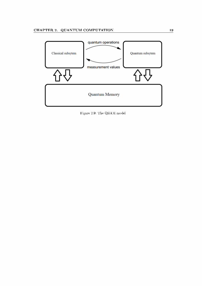
The classical side calls quantum operators from the quantum side which responds with resultsas measurement values, since classical computers cannot work with pure quantum states.A model similar to this hybrid approach is the Quantum Random Access Machine model,developed by Knill [16]. This model is a generalization of a classical Random Access Machinemodel in which the memory is composed of qubits instead of classical bits. As in the hybridmodel, we have a set of classical instructions and a set of quantum instructions. However, sincememory is entirely quantum mechanical, the only distinction between classical and quantumoperations is purely semantical [17]. This is done by making sure that all classical operationswill collapse (through measurement) the quantum registers on which they act.Our model is based on this QRAM approach. The entire virtual machine operates on quantuminformation. This means that storage is done strictly using qubits. Classical instructionsoperate on quantum registers, however, since these instructions are not invertible, we willalways measure the register, in the computational basis, before executing the instruction. Aftermeasurement, we will have a basis quantum state in the register, which can be treated like aclassical group of bits. This allows us to implements any classical instruction in the same wayit is implemented on a classical processor, the only restriction being that we must measure theregister beforehand, in order to process strictly basis states. A diagram representing the QRAMmodel can be seen in Figure 2.9.
CHAPTER 2. QUANTUM COMPUTATION 19
Figure 2.9: The QRAM model
Chapter 3
Quantum Virtual Machine
In this chapter our virtual machine is presented. We start with the subject of quantum pro-gramming, discussing existing quantum programming languages. We proceed do discuss ourquantum assembly language, QAL, giving a thorough description of the instruction set, archi-tecture and program structure.
3.1 Quantum programming language
A quantum programming language is a programming language which makes use of quantumoperations and data types. Such a language is useful in expressing quantum algorithms, assuch a representation is much more convenient than using quantum circuits and gates. Accord-ing to Bernhard Omer [21], author of Quantum Computation Language, any useful quantumprogramming language must be:
• constructive
• hardware independent
• provide arbitrary levels of abstraction
• integrate non-classical features at a semantic level
We dierentiate between imperative quantum programming languages and functional quantumprogramming languages. We will briey mention the existing languages of these two paradigms.
3.1.1 Imperative quantum languages
Imperative languages are programming languages in which statements are used to change aprogram state. Examples of classical, imperative programming languages are: C, C++, Java,Python etc. Current existing quantum imperative languages are:
• Quantum pseudocode - developed by Knill for the QRAM model, this was the rstformalization of a language used to describe quantum algorithms [16].
• QCL - also known as Quantum Computation Language, is the oldest and most popularquantum programming language. Its syntax is very similar to that of C. It is based onthe hybrid model and combines classical and quantum operations [21]. An example ofQCL code can be seen bellow:
20
CHAPTER 3. QUANTUM VIRTUAL MACHINE 21
operator z(quconst c) // Correct implementation of the Z-gatequreg q = c; // redeclare c as quregH(q); // transform into dual basisX(q); // X-rotation in dual basisH(q); // transform back into
// computational basis
This is an implementation of the Z gate.
• Q language - is a quantum language similar to QCL. It was implemented as an extensionto C++ and provides classes for basic quantum operations [4].
• qGCL - also known as the Quantum Guarded Command Language. It is based onGuarded Command Language created by Edsger Dijkstra [11].
3.1.2 Functional quantum languages
Functional programming is a stateless paradigm in which computations are performed usingfunction composition and recursion. The following are quantum functional languages:
• QFC and QPL - are two related quantum programming languages which dier only intheir syntax: QFC uses a ow chart syntax, while QPL uses a textual syntax. The owcontrol is classical in both languages, however, they can operate on both quantum andclassical data [25].
• QML - is a functional quantum language similar to and implemented in Haskell [3].
• Quantum lambda language - is based on lambda calculus which is a model of com-putation that extends lambda calculus with quantum operations. It is equivalent to thequantum Turing machine model [22].
3.2 Quantum assembly language
A quantum assembly language is a low-level quantum language designed for a specic architec-ture. Very few such languages exist as high-level languages receive much more attention. Thisis due to the fact that higher-level languages are easier to implement and easier to program. Aquantum assembly language must respect all imposed architectural considerations.While a quantum assembly language is low-level compared to the previously mentioned quan-tum programming languages, we still have an abstraction barrier. We have no knowledge aboutthe internals of the quantum hardware. There is no need to know how qubits are stored, initial-ized, manipulated or measured. We only operate at a level where we can assume the existence ofquantum registers, quantum memory and a quantum processor. A quantum assembly languagewill specify how these elements interact with each other and with other components, but noinformation on the inner workings of such components is provided.The quantum assembly language we have designed is called QAL. QAL is based on the QRAMmodel and is an imperative language. We proceed to discuss in detail the virtual machinearchitecture and QAL's instruction set.
3.2.1 QAL-VM architecture
The VM has seven general purpose quantum registers and one special register used to place re-turn values after function calls. Our assumption is that we are working with a 16−qubitarchitecture.

CHAPTER 3. QUANTUM VIRTUAL MACHINE 22
Consequently, each quantum register has two qubytes, or 16 qubits. A visual representation canbe seen in Figure 3.1.
Figure 3.1: The quantum register
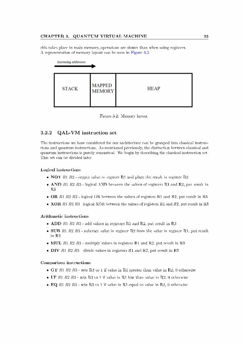
Registers store values using little endian ordering, with the left most qubit being the leastsignicant qubit.Since registers hold 16 qubits, we will have 216 or 65, 536 basis states, meaning that such aregister will be represented using 65, 536 complex amplitudes. All classical instruction willoperate using these basis states. This means that if a register is in a pure quantum states itwill be collapsed into a basis state before using it when executing a classical instruction. Allnumerical values are represented as unsigned integers using these basis states.The general purpose registers are used by both classical and quantum operations. They willstore the results of these operations regardless of whether it is a pure quantum state or a basisstate. Registers are identied as VRindex, where index is a value between 0 and 6. We alsohave a special register, denoted VR_RET, which is used to store the result of function calls.Since we are working with a 16-qubit architecture, the amount of addressable memory is limitedto 65, 536 qubytes. Memory is divided into three main segments, or runtime data areas:
• Stack segment - segment used for storing the program stack. The stack operates with16-qubit chunks of memory.
• Heap segment - area used for dynamic memory allocation.
• Mapped memory segment - a dedicated area of memory used to mimic an unlimitednumber of registers. This memory segment acts like a map data structure, mappingindices to memory locations.
Apart from these, we also have the code segment where the program instructions are storedand a data segment which species directives for storing high-level objects. In our implemen-tation, these segments are assumed not be in main memory. For this reason, when referring tomain memory we are in fact indicating the three main segments mentioned previously.This general architecture is inspired from that of classical computers. Alternative means ofrepresentation were considered, such as a stack machine, similar to the JVM. Such an approachwould not use registers for storing parameters and results of instructions but would insteadhave used multiple stacks for these tasks. We, however, consider that registers provide easierand more exible means of manipulating data. The idea of adding the mapped memory seg-ment illustrates this fact. It was inspired from three address code intermediate languages suchCOOL IR [1] which use an innite number of registers. Since our architecture attempts to beas close as possible to an actual hardware implementation, it is unrealistic to have an innitenumber of registers. For this reason, we have introduced the mapped memory segment whichis addressable through indices, similar to how registers are identied by index. Of course, since
CHAPTER 3. QUANTUM VIRTUAL MACHINE 23
this takes place in main memory, operations are slower than when using registers.A representation of memory layout can be seen in Figure 3.2.
Figure 3.2: Memory layout
3.2.2 QAL-VM instruction set
The instructions we have considered for our architecture can be grouped into classical instruc-tions and quantum instructions. As mentioned previously, the distinction between classical andquantum instructions is purely semantical. We begin by describing the classical instruction set.This set can be divided into:
Logical instructions
• NOT R1 R2 - negate value in register R1 and place the result in register R2
• AND R1 R2 R3 - logical AND between the values of registers R1 and R2, put result inR3
• OR R1 R2 R3 - logical OR between the values of registers R1 and R2, put result in R3
• XOR R1 R2 R3 - logical XOR between the values of registers R1 and R2, put result in R3
Arithmetic instructions
• ADD R1 R2 R3 - add values in registers R1 and R2, put result in R3
• SUB R1 R2 R3 - subtract value in register R2 from the value in register R1, put resultin R3
• MUL R1 R2 R3 - multiply values in registers R1 and R2, put result in R3
• DIV R1 R2 R3 - divide values in registers R1 and R2, put result in R3
Comparison instructions
• GT R1 R2 R3 - sets R3 to 1 if value in R1 greater than value in R2, 0 otherwise
• LT R1 R2 R3 - sets R3 to 1 if value in R1 less than value in R2, 0 otherwise
• EQ R1 R2 R3 - sets R3 to 1 if value in R1 equal to value in R2, 0 otherwise

CHAPTER 3. QUANTUM VIRTUAL MACHINE 24
Memory instructions
• LOAD R1 [R2 + offset] - load in R1 2 qubytes starting from memory address R2 +oset
• LOADB R1 [R2 + offset] - load in R1 1 qubyte starting from memory address R2 +oset
• STORE R1 [R2 + offset] - store at memory address R2 + oset the 2 qubytes in R1
• STOREB R1 [R2 + offset] - store at memory address R2 + oset the least signicantqubyte in R1
• NEW label R1 - allocate object of type label in memory, starting address placed inregister R1
• ALLOC R1 R2 - allocate R1 qubytes and return address of allocated area in R2
• PUT R1 R2 - put at index R1 the contents of register R2 in mapped memory
• GET R1 R2 - get from index R1 content and put it in register R2 from mapped memory
Jump instructions
• JUMP label - instruction pointer jumps to label, execution resumed from that point
• JUMPT label R1 - instruction pointer jumps to label if the value of register R1 is not 0
• JUMPF label R1 - instruction pointer jumps to label if the value of register R1 is 0
• CALL label - call function label, place result in R1. Saves current instruction pointer,jumps to label and continues execution from there. Result is placed in default register forfunction return value, VR_RET
• RET R1 - puts value of R1 in default register for function return value, then pops in-struction pointer from stack and resumes execution from that point. Can also be calledwithout argument R1 in which case it just pops instruction pointer from stack and re-sumes execution from that point
Stack instructions
• PUSH R1 - pushes value of register R1 onto the stack
• POP R1 - pops current stack value into register R1
Other instructions
• MOV R1 R2 - copy value from R1 into R2
• SHL R1 - shift qubits in R1 one position to the left
• SHR R1 - shift qubits in R1 one position to the right
As mentioned before, most of these classical instructions will collapse (through measurement)the registers on which they act before executing their specic operation. We say `most' becausethis is not true for memory and stack instructions. This makes sense, as we want to allowpure quantum states to exist in memory. If this were not the case, registers would be the onlymemory units allowing pure quantum states, thus drastically reducing the expressive power ofour quantum machine. Before discussing the restrictions of our classical instruction set, we willmention, without proving, two important theorems of quantum information theory [29]:
CHAPTER 3. QUANTUM VIRTUAL MACHINE 25
Theorem 3.2.1 (No-cloning Theorem) The creation of identical copies of an unknown quan-tum system is forbidden.
Theorem 3.2.2 (Quantum Teleportation Theorem) Quantum states can be transmitted exactlyfrom one location to another without disturbing these states or transmitting any qubits throughthe intervening space.
The no-cloning theorem seems to forbid the existence of the MOV instruction, which copiesthe content of one register into another. This is not the case, however, since the state of thequantum system we are copying is known because we have measured it before attempting tocopy the information. This means that we are always copying basis states, which is not for-bidden by the no-cloning theorem. Furthermore, because of the no-cloning theorem, memoryand stack instructions, which take information from registers and put it into main memory, willnever copy quantum states. This becomes an issue when implementing such as instructions aswe must make sure to empty registers or memory locations when transferring information fromone place to another.The quantum teleportation theorem imposes no restrictions and was mentioned in order toillustrate why it is possible to move quantum information from one place to another (dierentmemory locations, from registers into memory and viceversa) without disturbing pure quantumstates.We will now describe the quantum instruction set:
Quantum instructions
• QMOV R1 R2 - quantum teleports content of R1 into R2. R1 is now lled with zeros
• CNOT R1 - CNOT of least signicant qubyte in R1 using most signicant qubyte ascontrol
• CNOT2 R1 R2 - CNOT of qubits in R1, using qubits in R2 as control
• X R1 R2 - ip qubits in R1 using R2 as mask
• Y R1 R2 - rotation around Y axis of qubits in R1 using R2 as mask
• Z R1 R2 - phase ip qubits in R1 using R2 as mask
• T R1 R2 - apply a π/4 rotation of qubits in R1 using R2 as mask
• S R1 R2 - apply phase change of qubits in R1 using R2 as mask. Also known as√Z gate
• H R1 R2 - apply Hadamard transform to individual qubits in R1 using R2 as mask
• ROT R1 R2 R3 - apply rotation to qubits in register R1, using R2 as mask and R3 asangle (expressed in degrees)
• REV R1 - reverse order of qubits in R1
• SWAP R1 R2 - swap content of register R1 with the content of register R2
• SWAPB R1 - swap qubytes in R1
• MEAS R1 R2 - measure (collapse) in the computational basis qubits in R1 using R2 asmask
• RAND R1 - generates true random value (through quantum measurement) and placesit in R1
For all of these quantum instructions, except MEAS and RAND, we also have the inverseoperations (ICNOT, IX, IY etc). This highlights the fact that all quantum operations arereversible.
CHAPTER 3. QUANTUM VIRTUAL MACHINE 26
Apart from the instruction set, we also have a set of storage directives which can be used bya higher-level programming language for specifying the memory representation of prototypeobjects. This is inspired from the COOL IR language. The directives are:
Storage directives
• DW number - store a two-qubyte unsigned integer
• DL label - store a the numerical value of a label
• DB number - store a qubyte unsigned integer
• DB “string′′ - store a string as a vector of qubytes which represent the characters
• DS N - allocate N qubytes of memory
QAL is equivalent to the quantum gates model. This fact is obvious since all universal gatesare included in our instruction set and these gates can be applied an arbitrary number of timesto any qubit of main memory. This can be done indirectly through quantum operations andmemory operations (i.e. we can apply quantum gates to the qubits in registers and then storethem in main memory).Quantum instructions together with memory operations allow us to create superpositions andentanglements in main memory. This means that it is possible to have chunks of memoryentangled amongst themselves or with the registers. Collapsing such a chunk, or a registerwill lead to the collapse of the other `side' of the entanglement. For our implementation, thismeans that we must have a global memory state associated with every storage unit (memoryand registers). This is discussed in detail in the next chapter.
3.2.3 QAL syntax
QAL programs have two segments:
• .code - is the rst segment. All programs must begin with the .code segment. Thissegment species the program to be executed in terms of QAL instructions. Labels,instructions and function denitions are permitted here. The .code segment is immediatelyfollowed by the .data segment.
• .data - is the second segment. Here we have storage directives for various objects denedin a high-level quantum language.
Functions are dened in the .code segment between the .function name, in, out and .enddirectives which act as delimiters for function code. Every function must have an associatedlabel, following the .function directive, which is used by the CALL instruction.Single-line comments can be added. They must be preceded by the `#' character. For anexample program, consult Listing A.1.

Chapter 4
Implementation and testing
This chapter will discuss our implementation of the VM as well as the validation tests that wereperformed. We have used the Java programming language for our implementation. The rstpart gives a general description of how the VM is implemented and then discusses the details ofrepresenting quantum information. We proceed to talk about the approach used for represent-ing registers and main memory. The second part deals with how instructions are interpreted.In each part we also talk about how that specic element was tested.
4.1 General description
The essence of the virtual machine is the interpreter, the component which takes instructionsand executes them. The main interpreter loop of the JVM is shown in Listing 4.1 [24].
1 for (;;) 2 instr = bcode[pc++];3 switch (instr) 4 ...5 case IADD:6 tos = stack[sp]+stack[sp-1];7 --sp;8 stack[sp] = tos;9 break;
10 ...11 12
Listing 4.1: JVM main interpreter loop
In our implementation, the main control loop makes use of a ow control object. This objectis used to control the instruction pointer. For most instructions, the IP is simply incremented,however jump instructions will utilize the ow control object in order to send the instructionpointer to the appropiate address. We also ilustrate the main interpreter loop of our implemen-tation in Listing 4.2.
27
CHAPTER 4. IMPLEMENTATION AND TESTING 28
1 Instruction current = flow.getNextInstruction();2 while (current != null) 3 current.execute(flow);4 current = flow.getNextInstruction();5
Listing 4.2: QAL-VM main interpreter loop
Instructions are read from a QAL program le. The le is in text format. We considered thatit is not necessay to encode instructions since memory is represented using qubits and as such,instructions would have to encoded as qubits. This is impractical and beyond the scope ofthis project. We are mainly concerned with how memory is represented and how instructionsare executed. Moreover, we demonstrate the power of quantum computing by showing howquantum operations can be used to solve a problem in less time than would be needed byusing classical operations. This is done by implementing a virtual time keeping system andassociating various durations for each instruction.
4.2 Memory representation
4.2.1 Quantum information
As previously mentioned, quantum states are represented as vectors in a complex vector space.This is the representation we have chosen as well. A group of N qubits is represented as a 2N
vector of complex amplitudes. Considering the exponential increase in number of amplitudeswith the increasing number of qubits and the fact that, in general, most of these amplitudes willbe of norm zero, it makes more sense to only retain basis states and amplitudes for non-zerocomponents. For this reason, it is more ecient to retain a list of pairs (basis state, amplitude)as oposed to a vector with 2N components. Consider the following state:
ψ =1√2|00000000〉+
1√2|00000001〉
Using the vector approach, storing this state would look like this:
[|00000000〉 , 1√2, |00000001〉 , 1√
2, |00000010〉 , 0...|11111111〉 , 0]
The list approach is just: [|00000000〉 , 1√2, |00000001〉 , 1√
2].
4.2.2 Registers and main memory
Initially, we believed that registers and memory can be treated separately. This would meanrepresenting registers like any other quantum state using 65, 536 amplitudes. Of course, asmentioned above, we would use a list to only store non-zero amplitudes. Additonally, memorycould be represented as a vector, or list of qubytes, each represented in a similar manner tothe registers. This approach proved to be incorrect. The reason is that entanglement does notallow us to represent a quantum state using its individual components, but only as a whole.Therefore, the approach we have used is to consider main memory and the registers as a singlequantum state. This is more or less equivalent to appending the registers to the main mem-ory (outside of the addressable region). This allows us to represent any kind of entanglementbetween parts of memory, registers or both. We will refer to this single quantum state as theglobal memory state. Concretely, this global memory state is a list containing the basis states

CHAPTER 4. IMPLEMENTATION AND TESTING 29
having non-zero amplitudes and their corresponding amplitudes. The number of qubits in abasis state is:
basis state size = [Number of stack qubits + Number of mapped memory qubits + Number ofheap qubits + (Number of registers) * (Number of register qubits)] = 524,416 qubits
Storing the global memory state is a complicated task, especially if memory becomes `tooentangled'. Memory requirements can increase drastically if we introduce a large number ofentangled states. A graphical representation of memory entanglements can be seen in Figure 4.1.
Figure 4.1: Entanglements in memory
The problems associated with simulating quantum systems are common to any implementationand start with the exponential spatial requirements of storing quantum states. The theoreticalmaximum number of amplitudes we could reach, if the entire memory were placed in a superpo-sition, is 2524,416, which is greater than the total number of particles in the observable universe.Other approaches to representing memory are to use a graph data structure in which nodes arememory locations and edges indicate entangled states. This approach, while more satisfactoryin terms of memory usage, makes it dicult to implement the application of operators to quan-tum states.Our approach relies on the fact that we are always operating with single-qubit and two-qubitgates. Therefore, at most, we only need to perform computations which involve 4× 4 matrices.It is the user's task to construct any quantum operator using two-level operators and CNOT,since we know this is possible using universal gates, which are all present in our language.
4.3 Instructions
As mentioned earlier, instructions can be classied as classical instructions or quantum instruc-tions. Since each of these implies a dierent approach in implementation we will treat themseparately.
CHAPTER 4. IMPLEMENTATION AND TESTING 30
4.3.1 Classical instructions
Classical instructions always operate on basis states. This is advantageous because collapsingqubits from the global memory state will reduce its size and thus the amount of physical memoryrequired to represent it. The steps taken when collapsing a register are the following:
• Identify the specied register from the global memory state
• Compute probabilities associated with each amplitude of the register's basis states
• Choose a random basis state in accordance with the computed probabilities
• Compute the new global memory state. This involves leaving only the amplitudes match-ing the selected basis state of the register and dividing them by the norm
We shall exemplify this procedure with the following simplied situation. Suppose the globalmemory state1 is:
|ψM 〉 =1
2|0000, 0000, 0000〉+ 1
2|1100, 1010, 0000〉+ 1
2|0000, 0000, 0011〉+ 1
2|0000, 1111, 1000〉 2
The register we would like to measure is represented by the last four qubits of |ψM 〉. We seethat the possible states in which we can nd it are: |0000〉, |0011〉 or |1000〉. The correspondingprobabilities will be: (1/2)2 + (1/2)2 = 1/2, 1/4 and 1/4 respectively. We perform a measure-ment and nd the register in the basis state |0000〉. We thus eliminate the states of |ψM 〉 thatare incompatible with our measurement. This leaves:
|ψM 〉 =1
2|0000, 0000, 0000〉+
1
2|1100, 1010, 0000〉
This is not correct since the norm is 1/2. We proceed to normalize this state and obtain thecorrect post-measurement state:
|ψM 〉 =1√2|0000, 0000, 0000〉+
1√2|1100, 1010, 0000〉
This procedure is performed for all classical instructions, except the ones involving memoryoperations. After the register has been measured we can now implement our instructions aswe would on a classical machine. For example, AND simply involves performing a logical ANDbetween its two arguments and placing the result in the the result register. Note that we alsomeasure that register before changing its content.
4.3.2 Quantum instructions
Quantum instructions are associated with unitary operations. As observed in Subsection 3.2.2,most quantum instructions receive a target register and a mask. The target register, the rstargument, is the one on which we wish to apply quantum operators. The second argument, themask, is a basis state which species the qubits of the target register on which we will apply thequantum operator associated with the current instruction. An example is given in Listing 4.3.As mentioned, we are using little endian representation.
1It is impractical to represent the global memory state with 524,416-qubit states so we are using this simpliedmodel
2Here we are assuming that |x, y, z〉 = |xyz〉. The notation serves to separate specic portions of the globalmemory state (registers, heap etc).
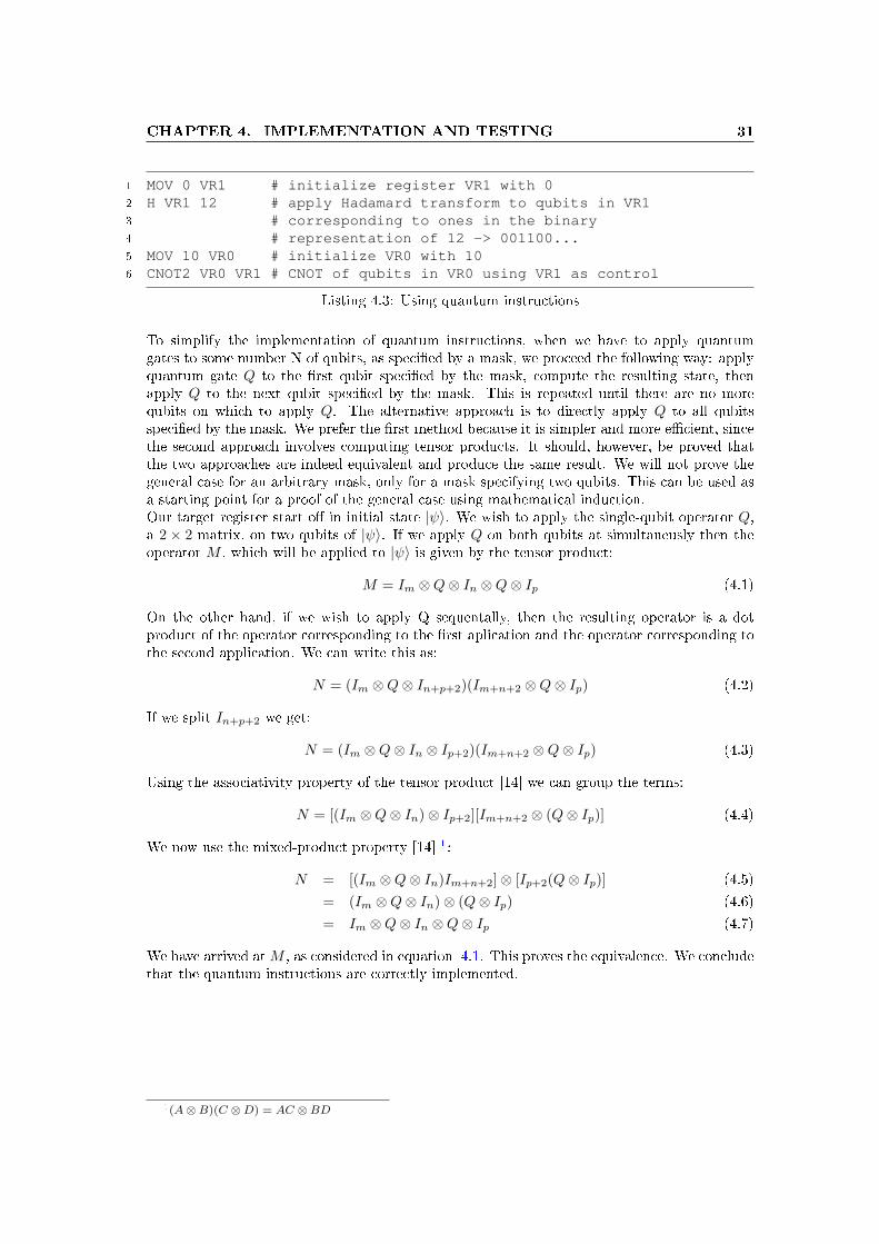
CHAPTER 4. IMPLEMENTATION AND TESTING 31
1 MOV 0 VR1 # initialize register VR1 with 02 H VR1 12 # apply Hadamard transform to qubits in VR13 # corresponding to ones in the binary4 # representation of 12 -> 001100...5 MOV 10 VR0 # initialize VR0 with 106 CNOT2 VR0 VR1 # CNOT of qubits in VR0 using VR1 as control
Listing 4.3: Using quantum instructions
To simplify the implementation of quantum instructions, when we have to apply quantumgates to some number N of qubits, as specied by a mask, we proceed the following way: applyquantum gate Q to the rst qubit specied by the mask, compute the resulting state, thenapply Q to the next qubit specied by the mask. This is repeated until there are no morequbits on which to apply Q. The alternative approach is to directly apply Q to all qubitsspecied by the mask. We prefer the rst method because it is simpler and more ecient, sincethe second approach involves computing tensor products. It should, however, be proved thatthe two approaches are indeed equivalent and produce the same result. We will not prove thegeneral case for an arbitrary mask, only for a mask specifying two qubits. This can be used asa starting point for a proof of the general case using mathematical induction.Our target register start o in initial state |ψ〉. We wish to apply the single-qubit operator Q,a 2 × 2 matrix, on two qubits of |ψ〉. If we apply Q on both qubits at simultaneusly then theoperator M , which will be applied to |ψ〉 is given by the tensor product:
M = Im ⊗Q⊗ In ⊗Q⊗ Ip (4.1)
On the other hand, if we wish to apply Q sequentally, then the resulting operator is a dotproduct of the operator corresponding to the rst aplication and the operator corresponding tothe second application. We can write this as:
N = (Im ⊗Q⊗ In+p+2)(Im+n+2 ⊗Q⊗ Ip) (4.2)
If we split In+p+2 we get:
N = (Im ⊗Q⊗ In ⊗ Ip+2)(Im+n+2 ⊗Q⊗ Ip) (4.3)
Using the associativity property of the tensor product [14] we can group the terms:
N = [(Im ⊗Q⊗ In)⊗ Ip+2][Im+n+2 ⊗ (Q⊗ Ip)] (4.4)
We now use the mixed-product property [14] 1:
N = [(Im ⊗Q⊗ In)Im+n+2]⊗ [Ip+2(Q⊗ Ip)] (4.5)
= (Im ⊗Q⊗ In)⊗ (Q⊗ Ip) (4.6)
= Im ⊗Q⊗ In ⊗Q⊗ Ip (4.7)
We have arrived atM , as considered in equation 4.1. This proves the equivalence. We concludethat the quantum instructions are correctly implemented.
1(A⊗B)(C ⊗D) = AC ⊗BD
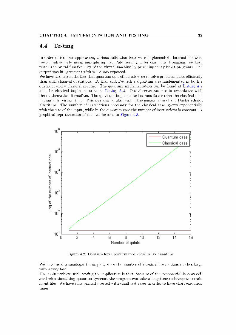
CHAPTER 4. IMPLEMENTATION AND TESTING 32
4.4 Testing
In order to test our application, various validation tests were implemented. Instructions weretested individually using multiple inputs. Additionally, after complete debugging, we havetested the overal functionality of the virtual machine by providing many input programs. Theoutput was in agreement with what was expected.We have also tested the fact that quantum operations allow us to solve problems more ecientlythan with classical operations. To that end, Deutsch's algorithm was implemented in both aquantum and a classical manner. The quantum implementation can be found at Listing A.2and the classical implementation at Listing A.3. Our observations are in accordance withthe mathematical formalism. The quantum implementation runs faster than the classical one,measured in virtual time. This can also be observed in the general case of the Deutsch-Jozsaalgorithm. The number of instructions necessary for the classical case, grows exponentiallywith the size of the input, while in the quantum case the number of instructions is constant. Agraphical representation of this can be seen in Figure 4.2.
Figure 4.2: Deutsch-Jozsa performance, classical vs quantum
We have used a semilogarithmic plot, since the number of classical instructions reaches largevalues very fast.The main problem with testing the application is that, because of the exponential leap associ-ated with simulating quantum systems, the program can take a long time to interpret certaininput les. We have thus primarly tested with small test cases in order to have short executiontimes.
Chapter 5
Conclusions and future work
In this thesis, we have presented our implementation of the quantum computing virtual machine,QAL-VM. The instruction set considered is equivalent to the quantum gates model of quantumcomputing allowing us to represent any quantum circuit with arbitrary accuracy. We haveobserved how quantum algorithms, for specic cases of the hidden subgroup problem, surpasstheir classical counterparts in terms of performance, in accordance with the theoretical results.Our program is a research tool which can be used in studying such algorithms. It can alsobe utilized in conjunction with a quantum compiler, that produces QAL code, for executingprograms generated from a high-level programming language.In the future, we would to like implement a garbage collection algorithm for automatic memorymanagement. This presents a challenge because of the entanglements which can form in memoryas well as the presence of pure quantum states which cannot be inspected unless measured.Disturbing such quantum states, as a result of garbage collection, can lead to incorrect resultsfor programs which rely on those states. This can be seen as a form of decoherence, which wewish to avoid.Other features which can be added in future implementations are: communication instructions,which would exploit quantum properties to eciently send and receive quantum information,and multithreading. These features open the possibility of parallel and distributed quantumalgorithms, an area of research which, at this time, is still in its early days.Quantum computing oers us interesting perspectives for the future. Its immense benetsin terms of eciency cannot be ignored. Therefore, we must have a quantum programmingframework prepared and a thorough understanding of quantum algorithms for the time whenpersonal quantum computers become a reality, bringing the next big revolution in the computerindustry.In closing, we end with a quote by Richard Feynman: Nature uses only the longest threadsto weave her patterns, so each small piece of her fabric reveals the organization of the entiretapestry.
33
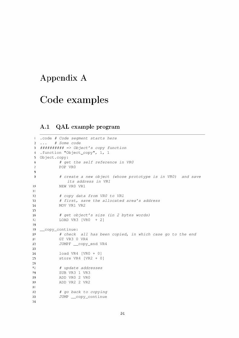
Appendix A
Code examples
A.1 QAL example program
1 .code # Code segment starts here2 ... # Some code3 ########## => Object’s copy function4 .function "Object copy", 1, 15 Object.copy:6 # get the self reference in VR07 POP VR08
9 # create a new object (whose prototype is in VR0) and saveits address in VR1
10 NEW VR0 VR111
12 # copy data from VR0 to VR113 # first, save the allocated area’s address14 MOV VR1 VR215
16 # get object’s size (in 2 bytes words)17 LOAD VR3 [VR0 + 2]18
19 __copy_continue:20 # check all has been copied, in which case go to the end21 GT VR3 0 VR422 JUMPF __copy_end VR423
24 load VR4 [VR0 + 0]25 store VR4 [VR2 + 0]26
27 # update addresses28 SUB VR3 1 VR329 ADD VR0 2 VR030 ADD VR2 2 VR231
32 # go back to copying33 JUMP __copy_continue34
34
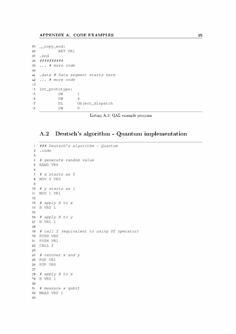
APPENDIX A. CODE EXAMPLES 35
35 __copy_end:36 RET VR137 .end38 ##########39 ... # more code40
41 .data # Data segment starts here42 ... # more code43
44 Int_prototype:45 DW 146 DW 447 DL Object_dispatch48 DW 0
Listing A.1: QAL example program
A.2 Deutsch's algorithm - Quantum implementation
1 ### Deutsch’s algorithm - Quantum2 .code3
4 # generate random value5 RAND VR66
7 # x starts as 08 MOV 0 VR09
10 # y starts as 111 MOV 1 VR112
13 # apply H to x14 H VR0 115
16 # apply H to y17 H VR1 118
19 # call f (equivalent to using Uf operator)20 PUSH VR021 PUSH VR122 CALL f23
24 # recover x and y25 POP VR126 POP VR027
28 # apply H to x29 H VR0 130
31 # measure x qubit32 MEAS VR0 133
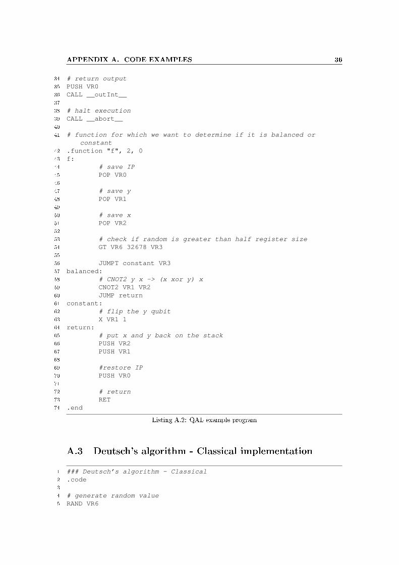
APPENDIX A. CODE EXAMPLES 36
34 # return output35 PUSH VR036 CALL __outInt__37
38 # halt execution39 CALL __abort__40
41 # function for which we want to determine if it is balanced orconstant
42 .function "f", 2, 043 f:44 # save IP45 POP VR046
47 # save y48 POP VR149
50 # save x51 POP VR252
53 # check if random is greater than half register size54 GT VR6 32678 VR355
56 JUMPT constant VR357 balanced:58 # CNOT2 y x -> (x xor y) x59 CNOT2 VR1 VR260 JUMP return61 constant:62 # flip the y qubit63 X VR1 164 return:65 # put x and y back on the stack66 PUSH VR267 PUSH VR168
69 #restore IP70 PUSH VR071
72 # return73 RET74 .end
Listing A.2: QAL example program
A.3 Deutsch's algorithm - Classical implementation
1 ### Deutsch’s algorithm - Classical2 .code3
4 # generate random value5 RAND VR6
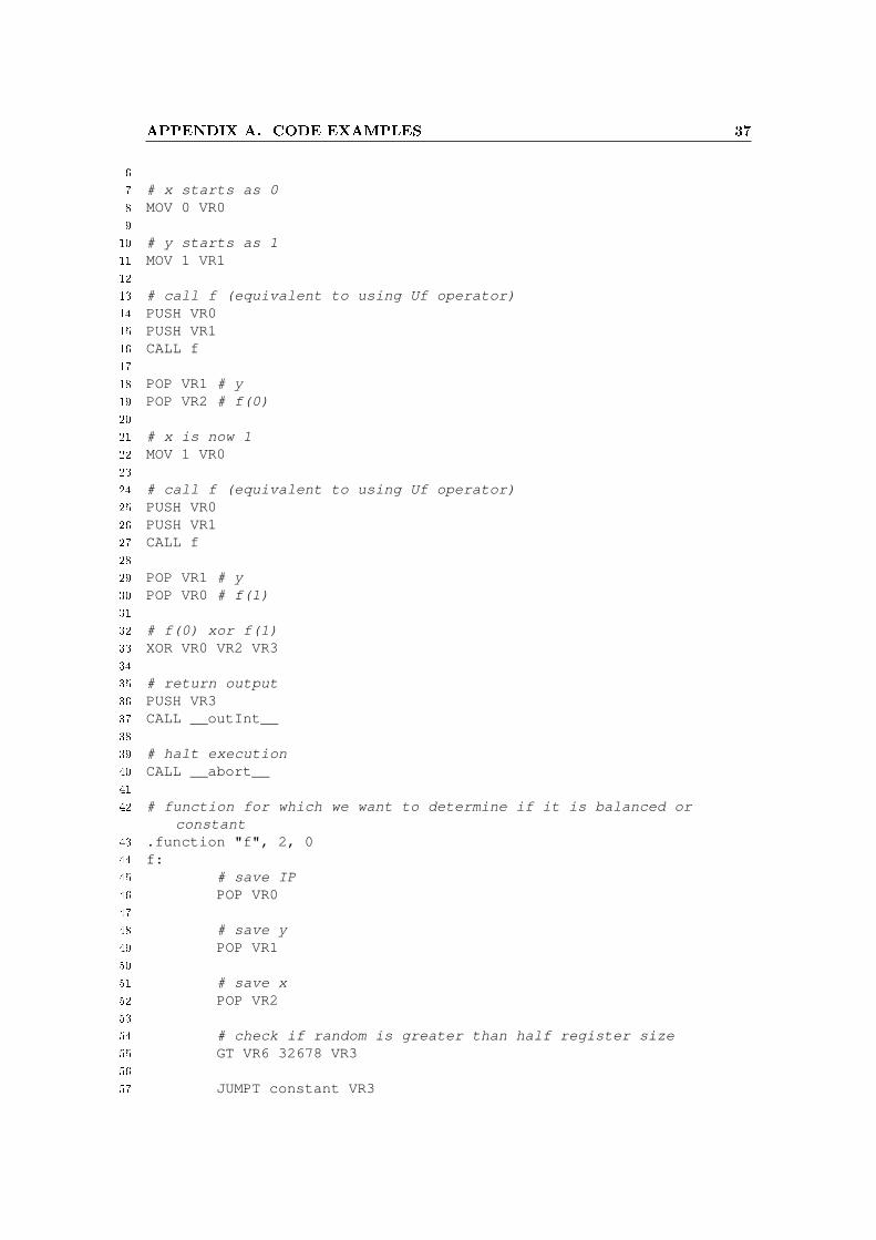
APPENDIX A. CODE EXAMPLES 37
6
7 # x starts as 08 MOV 0 VR09
10 # y starts as 111 MOV 1 VR112
13 # call f (equivalent to using Uf operator)14 PUSH VR015 PUSH VR116 CALL f17
18 POP VR1 # y19 POP VR2 # f(0)20
21 # x is now 122 MOV 1 VR023
24 # call f (equivalent to using Uf operator)25 PUSH VR026 PUSH VR127 CALL f28
29 POP VR1 # y30 POP VR0 # f(1)31
32 # f(0) xor f(1)33 XOR VR0 VR2 VR334
35 # return output36 PUSH VR337 CALL __outInt__38
39 # halt execution40 CALL __abort__41
42 # function for which we want to determine if it is balanced orconstant
43 .function "f", 2, 044 f:45 # save IP46 POP VR047
48 # save y49 POP VR150
51 # save x52 POP VR253
54 # check if random is greater than half register size55 GT VR6 32678 VR356
57 JUMPT constant VR3
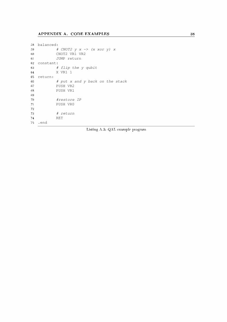
APPENDIX A. CODE EXAMPLES 38
58 balanced:59 # CNOT2 y x -> (x xor y) x60 CNOT2 VR1 VR261 JUMP return62 constant:63 # flip the y qubit64 X VR1 165 return:66 # put x and y back on the stack67 PUSH VR268 PUSH VR169
70 #restore IP71 PUSH VR072
73 # return74 RET75 .end
Listing A.3: QAL example program
Bibliography
[1] http://elf.cs.pub.ro/cpl/wiki/resurse/coolir.
[2] http://mathworld.wolfram.com/numbereldsieve.html.
[3] http://sneezy.cs.nott.ac.uk/qml/.
[4] http://sra.itc.it/people/serani/qlang/.
[5] http://www.dwavesys.com/.
[6] N. Rosen A. Einstein, B. Podolsky. Can quantum-mechanical description of physical realitybe considered complete? Physical Review, 47(10):777780, 1935.
[7] Scott Aaronson. Quantum Computing since Democritus. Cambride University Press, 2013.
[8] Gary E. Bowman. Essential Quantum Mechanics. Oxford University Press, 2008.
[9] David Deutsch. Quantum theory, the church-turing principle and the universal quantumcomputer. Proceedings of the Royal Society of London; Series A, Mathematical and PhysicalSciences, 400(1818), 1985.
[10] David Deutsch and Richard Jozsa. Rapid solutions of problems by quantum computation.Proceedings of the Royal Society of London A, 439(1907):553558, 1992.
[11] E. W. Dijkstra. Guarded commands, nondeterminacy and the formal derivation of pro-grams. CACM, 1975.
[12] Manek Dubash. Moore's law is dead, says gordon moore. Techworld, April 2005.
[13] M. W. Johnson et al. Quantum annealing with manufactured spins. Nature, 473:194198,2011.
[14] H. Eves. Elementary Matrix Theory. Dover publications, 1980.
[15] Richard P. Feynman. Simulating physics with computers. International Journal of Theo-retical Physics, 21(6/7), 1982.
[16] E. Knill. Conventions for quantum pseudocode, 1996.
[17] Jaros law Adam Miszczak. Models of quantum computation and quantum programminglanguages, 2011.
[18] Gregory Breyta Costantino S. Yannoni Mark H. Sherwood M. K. Lieven Vandersypen,Matthias Steen and Isaac L. Chuang.
[19] Gordon E. Moore. Cramming more components onto integrated circuits. Electronics, 38(8),1965.
[20] Michael A. Nielsen and Isaac L. Chuang. Quantum Computation and Quantum Informa-tion. Cambridge University Press, 10 edition, 2010.
39
BIBLIOGRAPHY 40
[21] Bernhard Omer. Structured quantum programming, 2009.
[22] Benoit Valiron Peter Selinger. Quantum lambda calculus.
[23] Gerald J. Popek and Robert P. Goldberg. Formal requirements for virtualizable thirdgeneration architectures. Communications of the ACM, 17(7), 1974.
[24] Martin Schoeberl. JOP: A Java Optimized Processor for Embedded Real-Time Systems.PhD thesis, Vienna University of Technology, 2005.
[25] P. Selinger. A brief survey of quantum programming languages, 2004.
[26] James Smith and Ravi Nair. The architecture of virtual machines. Computer (IEEEComputer Society), 38(5), 2005.
[27] Gilad Bracha Tim Lindholm, Frank Yellin and Alex Buckley. The Java Virtual MachineSpecication. Java SE 7 Edition. Oracle America, Inc, 2011.
[28] A. M. Turing. On computable numbers, with an application to the entscheidungs problem.Proceedings of the London Mathematical Society, 42:230265, 1937.
[29] Umesh V. Vazirani. Quantum mechanics and quantum computation.https://class.coursera.org/qcomp-2012-001, 2012.
[30] Noson S. Yanofsky and Mirco A. Mannucci. Quantum Computing for Computer Scientists.Cambridge University Press, 2008.