
lss.fnal.govlss.fnal.gov/archive/thesis/1900/fermilab-thesis-1997-01.pdfCon ten ts List of Figures::...
297
Fermilab FERMILAB-THESIS-1997-01
Transcript of lss.fnal.govlss.fnal.gov/archive/thesis/1900/fermilab-thesis-1997-01.pdfCon ten ts List of Figures::...

Fermilab FERMILAB-THESIS-1997-01
UNIVERSITY OF CALIFORNIA
IRVINE
Observation of Relativistic
Antihydrogen Atoms
DISSERTATION
submitted in partial satisfaction of the requirements for the degree of
DOCTOR OF PHILOSOPHY
in Physics
by
Glenn DelFosse Blanford Jr.
Dissertation Comittee:
Professor Jonas Schultz, co-Chair
Professor Mark A. Mandelkern, co-Chair
Professor Dennis Silverman
1997

c 1997 by Glenn DelFosse Blanford, Jr.
All rights reserved.

The dissertation of Glenn DelFosse Blanford, Jr. is approved,
and is acceptable in quality and form
for publication on micro�lm:
Committee Chair
University of California, Irvine
1997
ii

To
my father and mother,
Glenn and Florence
Blanford
iii

Contents
List of Figures : : : : : : : : : : : : : : : : : : : : : : : : : : : : : : : : : : vii
List of Tables : : : : : : : : : : : : : : : : : : : : : : : : : : : : : : : : : : : xii
Acknowledgements : : : : : : : : : : : : : : : : : : : : : : : : : : : : : : : xiii
Curriculum Vitae : : : : : : : : : : : : : : : : : : : : : : : : : : : : : : : : xv
Abstract : : : : : : : : : : : : : : : : : : : : : : : : : : : : : : : : : : : : : : xvi
Chapter 1 Theoretical Motivation : : : : : : : : : : : : : : : : : : : : 1
1.1 Introduction . . . . . . . . . . . . . . . . . . . . . . . . . . . . . . . . 11.2 Production Processes . . . . . . . . . . . . . . . . . . . . . . . . . . . 6
1.2.1 Radiative Recombination . . . . . . . . . . . . . . . . . . . . . 81.2.2 Laser Stimulated Radiative Capture . . . . . . . . . . . . . . . 91.2.3 The 3-body Process, �pe+e+ ! �He+ . . . . . . . . . . . . . . . 101.2.4 Using Positronium . . . . . . . . . . . . . . . . . . . . . . . . 101.2.5 Antiprotonic Helium . . . . . . . . . . . . . . . . . . . . . . . 10
1.3 Production at Relativistic Energies . . . . . . . . . . . . . . . . . . . 111.4 The CERN PS210 Experiment at LEAR . . . . . . . . . . . . . . . . 21
Chapter 2 Antiproton Beam and Target : : : : : : : : : : : : : : : : 24
2.1 Antiproton Accumulator . . . . . . . . . . . . . . . . . . . . . . . . . 242.1.1 Antiproton Production and Cooling . . . . . . . . . . . . . . . 242.1.2 Deceleration Procedure . . . . . . . . . . . . . . . . . . . . . . 272.1.3 Energy Measurement . . . . . . . . . . . . . . . . . . . . . . . 29
2.2 Gas Jet Target . . . . . . . . . . . . . . . . . . . . . . . . . . . . . . 322.3 Charmonium Program . . . . . . . . . . . . . . . . . . . . . . . . . . 372.4 Luminosity . . . . . . . . . . . . . . . . . . . . . . . . . . . . . . . . 39
Chapter 3 The E862 Positron Spectrometer : : : : : : : : : : : : : : 42
3.1 E862 Detectors . . . . . . . . . . . . . . . . . . . . . . . . . . . . . . 423.2 Foil Stripper . . . . . . . . . . . . . . . . . . . . . . . . . . . . . . . . 453.3 Radioactive Sources . . . . . . . . . . . . . . . . . . . . . . . . . . . . 483.4 Antihydrogen Beam Parameters . . . . . . . . . . . . . . . . . . . . . 493.5 Positron Magnets . . . . . . . . . . . . . . . . . . . . . . . . . . . . . 52
3.5.1 Design and Simulations . . . . . . . . . . . . . . . . . . . . . . 523.5.2 Construction of Magnets . . . . . . . . . . . . . . . . . . . . . 57
iv

3.5.3 Magnetic Field Properties . . . . . . . . . . . . . . . . . . . . 58
3.5.4 Beam Test Apparatus . . . . . . . . . . . . . . . . . . . . . . 59
3.5.5 Monoenergetic Electron Source Testing . . . . . . . . . . . . . 60
3.6 Positron Detectors . . . . . . . . . . . . . . . . . . . . . . . . . . . . 67
3.6.1 Positron Counter . . . . . . . . . . . . . . . . . . . . . . . . . 68
3.6.2 Sodium Iodide(Tl) Gamma Ray Detector . . . . . . . . . . . . 70
3.6.3 Positron Source Testing . . . . . . . . . . . . . . . . . . . . . 73
3.7 Veto Counters and Shielding . . . . . . . . . . . . . . . . . . . . . . . 81
3.8 Aperture Changes . . . . . . . . . . . . . . . . . . . . . . . . . . . . . 82
Chapter 4 The E862 Antiproton Spectrometer : : : : : : : : : : : : 86
4.1 Time of Flight . . . . . . . . . . . . . . . . . . . . . . . . . . . . . . . 86
4.2 Antiproton momentum measurement . . . . . . . . . . . . . . . . . . 92
4.2.1 Wire Chamber Description . . . . . . . . . . . . . . . . . . . . 92
4.2.2 Momentum Resolution . . . . . . . . . . . . . . . . . . . . . . 98
4.3 Antiproton Beamline Alignment . . . . . . . . . . . . . . . . . . . . . 99
Chapter 5 Trigger and Data Acquisition : : : : : : : : : : : : : : : : 103
5.1 Experiment Trigger . . . . . . . . . . . . . . . . . . . . . . . . . . . . 103
5.2 Data acquisition . . . . . . . . . . . . . . . . . . . . . . . . . . . . . . 106
5.3 Target and Magnet Control . . . . . . . . . . . . . . . . . . . . . . . 107
Chapter 6 Data Analysis : : : : : : : : : : : : : : : : : : : : : : : : : : 111
6.1 Introduction . . . . . . . . . . . . . . . . . . . . . . . . . . . . . . . . 111
6.2 Antiproton beam data . . . . . . . . . . . . . . . . . . . . . . . . . . 112
6.3 Track Reconstruction . . . . . . . . . . . . . . . . . . . . . . . . . . . 117
6.4 Antiproton Background Tracks . . . . . . . . . . . . . . . . . . . . . 125
6.5 Secondary Backgrounds . . . . . . . . . . . . . . . . . . . . . . . . . 131
6.6 Foil Target-In Data . . . . . . . . . . . . . . . . . . . . . . . . . . . . 133
6.6.1 Description of Foil-In Data . . . . . . . . . . . . . . . . . . . . 133
6.6.2 Foil-In Momentum Distributions . . . . . . . . . . . . . . . . . 134
6.6.3 Pro�les at foil . . . . . . . . . . . . . . . . . . . . . . . . . . . 137
6.6.4 Emittance Measurements . . . . . . . . . . . . . . . . . . . . . 140
6.6.5 Pro�les at jet . . . . . . . . . . . . . . . . . . . . . . . . . . . 143
6.6.6 Positron Energies and Annihilation Spectra . . . . . . . . . . 148
6.6.7 Timing Analysis . . . . . . . . . . . . . . . . . . . . . . . . . . 160
6.7 Foil Target-Out data . . . . . . . . . . . . . . . . . . . . . . . . . . . 169
6.7.1 Description of Foil-Out Data . . . . . . . . . . . . . . . . . . . 169
6.7.2 Jet Location . . . . . . . . . . . . . . . . . . . . . . . . . . . . 170
6.7.3 Momentum Distributions . . . . . . . . . . . . . . . . . . . . . 172
6.7.4 Background to Foil-out Candidates . . . . . . . . . . . . . . . 175
6.8 Event Selection Summary . . . . . . . . . . . . . . . . . . . . . . . . 178
v

Chapter 7 Geometrical Acceptance and E�ciencies : : : : : : : : : 180
7.1 Simulation of foil-out candidates . . . . . . . . . . . . . . . . . . . . . 1807.2 Simulation of positron beamline . . . . . . . . . . . . . . . . . . . . . 187
7.2.1 Transport Matrices . . . . . . . . . . . . . . . . . . . . . . . . 1887.2.2 Magnet Fields . . . . . . . . . . . . . . . . . . . . . . . . . . . 190
7.3 Simulation of antiproton momentum reconstruction . . . . . . . . . . 2097.4 E�ciencies . . . . . . . . . . . . . . . . . . . . . . . . . . . . . . . . . 211
7.4.1 Trigger E�ciencies . . . . . . . . . . . . . . . . . . . . . . . . 2117.4.2 Tracking E�ciency . . . . . . . . . . . . . . . . . . . . . . . . 2167.4.3 E�ciencies Summary . . . . . . . . . . . . . . . . . . . . . . . 218
Chapter 8 Results and Conclusions : : : : : : : : : : : : : : : : : : : 224
8.1 Observation of Antihydrogen Events . . . . . . . . . . . . . . . . . . 2248.2 Cross Section for 6 GeV/c . . . . . . . . . . . . . . . . . . . . . . . . 2328.3 Energy Dependence of the Cross Section . . . . . . . . . . . . . . . . 2378.4 Systematic Errors . . . . . . . . . . . . . . . . . . . . . . . . . . . . . 2458.5 Conclusions . . . . . . . . . . . . . . . . . . . . . . . . . . . . . . . . 247
Bibliography : : : : : : : : : : : : : : : : : : : : : : : : : : : : : : : : : : : 249
Appendix A Relativistic Cross Section Calculation : : : : : : : : : : 258
A.1 Photoelectric Matrix Element . . . . . . . . . . . . . . . . . . . . . . 258A.2 Cross Section Integration . . . . . . . . . . . . . . . . . . . . . . . . . 267
Appendix B Spectroscopy of Relativistic �H : : : : : : : : : : : : : : 270
B.1 Goals . . . . . . . . . . . . . . . . . . . . . . . . . . . . . . . . . . . . 270B.2 Unperturbed Spectrum . . . . . . . . . . . . . . . . . . . . . . . . . . 271B.3 Increasing the Production Rate . . . . . . . . . . . . . . . . . . . . . 271B.4 E�ect of Magnetic Fields . . . . . . . . . . . . . . . . . . . . . . . . . 273B.5 Observing n > 1 States . . . . . . . . . . . . . . . . . . . . . . . . . . 274B.6 Measuring a Lamb Shift in antihydrogen . . . . . . . . . . . . . . . . 275
vi

List of Figures
1.1 Phasor diagram showing CP and CPT violating parameters. . . . . . 31.2 Antihydrogen by pair production and e+ capture. . . . . . . . . . . . 131.3 Predicted antihydrogen production cross section vs. momentum. . . . 151.4 Energy distribution of electrons . . . . . . . . . . . . . . . . . . . . . 161.5 Theoretical cross section calculations in the range of energies available
to E862. . . . . . . . . . . . . . . . . . . . . . . . . . . . . . . . . . 191.6 Theoretical cross section calculations in a much higher range of energies. 201.7 Diagram of PS 210 apparatus [5]. . . . . . . . . . . . . . . . . . . . . 23
2.1 Placement of E862 equipment in the tunnel, to scale. . . . . . . . . . 252.2 Antiproton Source rings . . . . . . . . . . . . . . . . . . . . . . . . . 282.3 Density during stacking vs. orbit . . . . . . . . . . . . . . . . . . . . 292.4 Typical frequency histogram of the beam . . . . . . . . . . . . . . . . 312.5 Hydrogen jet transverse density pro�le . . . . . . . . . . . . . . . . . 332.6 Thermodynamic phase space of the hydrogen jet's molecules. . . . . . 342.7 Jet-beam intersection . . . . . . . . . . . . . . . . . . . . . . . . . . . 352.8 Jet target cluster formation, pumps, and chamber dimensions . . . . 362.9 Charmonium spectrum . . . . . . . . . . . . . . . . . . . . . . . . . . 382.10 E835 luminosity monitor angle de�nition . . . . . . . . . . . . . . . . 402.11 E835 luminosity monitor spectrum . . . . . . . . . . . . . . . . . . . 402.12 Expected production cross section and integrated luminosity . . . . . 41
3.1 Schematic of E862 beamline elements. . . . . . . . . . . . . . . . . . . 433.2 Cross section for stripping H0 (cm2) . . . . . . . . . . . . . . . . . . 463.3 E�ciency for stripping H0 as a function of carbon foil thickness . . . 473.4 Vacuum box for target wheel. . . . . . . . . . . . . . . . . . . . . . . 483.5 Flying wire pro�les of antiproton beam . . . . . . . . . . . . . . . . . 523.6 Schematic of E862 beamline elements. . . . . . . . . . . . . . . . . . . 533.7 40o dipole for positrons showing anged edges at 10�. . . . . . . . . . 543.8 Diagram of entrance/exit angles for 40o bend dipole. . . . . . . . . . 553.9 Focusing solenoid diagram . . . . . . . . . . . . . . . . . . . . . . . . 553.10 Positron tracks (simulated with Transport) at nominal magnetic �eld. 573.11 Positron tracks (simulated) with �rst solenoid turned o� . . . . . . . 573.12 e+ magnetic �eld nonlinearity . . . . . . . . . . . . . . . . . . . . . . 583.13 Deionized water system in Lab 6. . . . . . . . . . . . . . . . . . . . . 613.14 Measured magnetic �eld of solenoid along axis. . . . . . . . . . . . . . 623.15 Dipole current scans e+ spectrometer . . . . . . . . . . . . . . . . . . 633.16 Solenoid current scans . . . . . . . . . . . . . . . . . . . . . . . . . . 63
vii

3.17 Scan over the dipole �eld for 207Bi after �nal setup in tunnel. . . . . . 663.18 Scan over the solenoid current for 207Bi after �nal setup in tunnel. . . 663.19 Vertical position scan, for high and low dispersion tunes . . . . . . . 683.20 Probability for an e+ annihilation in ight . . . . . . . . . . . . . . . 713.21 Diagram of sodium iodide detector . . . . . . . . . . . . . . . . . . . 733.22 High voltage plateaus for the sodium iodide counters. . . . . . . . . . 743.23 The �+ spectrum of 68Ge . . . . . . . . . . . . . . . . . . . . . . . . . 753.24 Gaussian �ts to e+ and NaI peaks. . . . . . . . . . . . . . . . . . . . 763.25 High dispersion, e+ pulse height vs ID . . . . . . . . . . . . . . . . . 773.26 Low dispersion, e+ pulse height vs ID . . . . . . . . . . . . . . . . . . 773.27 Widths of e+ pulse height distributions vs ID . . . . . . . . . . . . . . 783.28 Correlation of e+ annihilation ray energies in sodium iodide . . . . . . 783.29 e+ pulse height spectrum with 68Ge . . . . . . . . . . . . . . . . . . . 793.30 Compare gains of e+ plastic scintillators . . . . . . . . . . . . . . . . 803.31 High dispersion dipole scan. . . . . . . . . . . . . . . . . . . . . . . . 833.32 Low dispersion dipole scan. . . . . . . . . . . . . . . . . . . . . . . . 843.33 Vertical 207Bi source position scan. . . . . . . . . . . . . . . . . . . . 853.34 Positron beam crossing a chord of scintillator. . . . . . . . . . . . . . 85
4.1 Voltage divider for time of ight counters. . . . . . . . . . . . . . . . 884.2 Cosmic ray test time of ight counters . . . . . . . . . . . . . . . . . 884.3 The e�ect of time walk on pulse height di�erences . . . . . . . . . . . 894.4 Time resolution for short, (30 ft) cables . . . . . . . . . . . . . . . . . 894.5 Time resolution for longer, (80 ft) cables . . . . . . . . . . . . . . . . 904.6 High voltage plateaus for the time of ight counters. . . . . . . . . . . 904.7 Nonlinearity of one of the fast-TDC channels. . . . . . . . . . . . . . 914.8 Magnetic �eld nonlinearity as function of transverse dimension inside
an antiproton bend magnet . . . . . . . . . . . . . . . . . . . . . . . 934.9 Magnetic �eld nonlinearity as function of applied current inside an
antiproton bend magnet . . . . . . . . . . . . . . . . . . . . . . . . . 934.10 Preampli�er schematic for each PWC channel . . . . . . . . . . . . . 954.11 Breakdown showing the various planes of the wire chambers . . . . . 974.12 Typical transverse and time pro�les for test run . . . . . . . . . . . . 102
5.1 E862 trigger diagram. . . . . . . . . . . . . . . . . . . . . . . . . . . . 1055.2 Average rates from the counters as a function of instantaneous luminosity.1065.3 Data collection and control . . . . . . . . . . . . . . . . . . . . . . . . 1085.4 Target wheel control subsystem. . . . . . . . . . . . . . . . . . . . . . 110
6.1 Horizontal angle during the run . . . . . . . . . . . . . . . . . . . . . 1136.2 Vertical angle during the run . . . . . . . . . . . . . . . . . . . . . . . 1136.3 Horizontal emittance during the run . . . . . . . . . . . . . . . . . . . 1146.4 Vertical emittance during the run . . . . . . . . . . . . . . . . . . . . 1146.5 Beam centroid positions at foil vs time . . . . . . . . . . . . . . . . . 1156.6 Beam centroid positions at foil vs time . . . . . . . . . . . . . . . . . 1166.7 �2 distribution from �ts to space points . . . . . . . . . . . . . . . . . 118
viii

6.8 Number of tracks per event . . . . . . . . . . . . . . . . . . . . . . . 1196.9 Diagram showing how the residual in the bend plane is measured. . . 1196.10 Vertical track residuals for all one track events . . . . . . . . . . . . . 1206.11 Vertical track residuals for triple coincidence events . . . . . . . . . . 1206.12 Saturation of magnets during deceleration ramp . . . . . . . . . . . . 1226.13 PWC pro�les of all tracks . . . . . . . . . . . . . . . . . . . . . . . . 1236.14 PWC pro�les of high momentum, non-candidate events . . . . . . . . 1246.15 PWC pro�les of triple coincidence events. . . . . . . . . . . . . . . . . 1246.16 Track/beam momentum for foil-in events in runs 1-115. . . . . . . . . 1266.17 Track/beammomentumfor foil-in events in runs 1-115 above transition
energy. . . . . . . . . . . . . . . . . . . . . . . . . . . . . . . . . . . . 1266.18 Track/beammomentumfor foil-in events in runs 1-115 below transition
energy. . . . . . . . . . . . . . . . . . . . . . . . . . . . . . . . . . . . 1276.19 Diagram of elastic scattering . . . . . . . . . . . . . . . . . . . . . . . 1286.20 Correlation of beam momentum and momentum fraction . . . . . . . 1296.21 Correlation of beam momentum and momentum fraction . . . . . . . 1306.22 Track momentum/beam momentum for triple coincidence candidates 1356.23 Track momentum/beammomentumfor triple coincidence events, above
transition . . . . . . . . . . . . . . . . . . . . . . . . . . . . . . . . . 1366.24 Track momentum/beam momentum for triple coincidence events, be-
low transition . . . . . . . . . . . . . . . . . . . . . . . . . . . . . . . 1366.25 Foil position of all tracks . . . . . . . . . . . . . . . . . . . . . . . . . 1386.26 Foil position of triple coincidence events . . . . . . . . . . . . . . . . 1386.27 Foil position of high momentum tracks . . . . . . . . . . . . . . . . . 1396.28 E�ective size of the antihydrogen beam . . . . . . . . . . . . . . . . . 1396.29 X-Phase space plot of tracks for candidates. . . . . . . . . . . . . . . 1416.30 Y-Phase space plot of tracks for candidates. . . . . . . . . . . . . . . 1416.31 X-Phase space plot of tracks for all tracks. . . . . . . . . . . . . . . . 1426.32 Y-Phase space plot of tracks for all tracks. . . . . . . . . . . . . . . . 1426.33 X angular distributions . . . . . . . . . . . . . . . . . . . . . . . . . . 1446.34 Y angular distributions . . . . . . . . . . . . . . . . . . . . . . . . . . 1456.35 Extrapolated position of track at gas jet for triple coincidence events 1466.36 Extrapolated position of track at gas jet for all good tracks . . . . . . 1466.37 Extrapolated position of track at gas jet for triple coincidence events,
above transition . . . . . . . . . . . . . . . . . . . . . . . . . . . . . . 1476.38 Extrapolated position of track at gas jet for triple coincidence events,
below transition . . . . . . . . . . . . . . . . . . . . . . . . . . . . . . 1476.39 e+ pulse height vs e+ momentum for candidates . . . . . . . . . . . . 1496.40 e+ pulse height vs e+ momentum for candidates . . . . . . . . . . . . 1496.41 Deviation of e+ pulse heights from �t for 1996 triple coincidences . . 1506.42 Deviation of e+ pulse heights from �t for 1997 triple coincidences . . 1506.43 e+ pulse heights for triple coincidence events . . . . . . . . . . . . . . 1526.44 e+ pulse heights for triple coincidence events, corrected for beam mo-
mentum dependence . . . . . . . . . . . . . . . . . . . . . . . . . . . 1536.45 Comparison of e+ pulse heights for triple coincidences and all events . 154
ix

6.46 Correlation of e+ annihilation ray energies in sodium iodide for cali-bration data . . . . . . . . . . . . . . . . . . . . . . . . . . . . . . . . 156
6.47 Correlation of annihilation X ray energies in NaI detector for all eventsin data. . . . . . . . . . . . . . . . . . . . . . . . . . . . . . . . . . . 156
6.48 Correlation of annihilation X ray energies in NaI detector for candidateevents in data. . . . . . . . . . . . . . . . . . . . . . . . . . . . . . . . 157
6.49 Annihilation X ray energy distributions from the NaI detector for allevents in foil-in data. . . . . . . . . . . . . . . . . . . . . . . . . . . . 158
6.50 Annihilation X ray energy distributions from the NaI detector for triplecoincidence events in foil-in data. . . . . . . . . . . . . . . . . . . . . 159
6.51 Correlation of TF11 arrival times with horizontal position. . . . . . . 1626.52 Correlation of TF11 arrival times with ADC TF11 after removing po-
sition dependence. . . . . . . . . . . . . . . . . . . . . . . . . . . . . 1626.53 Correlation of TF11 arrival times with ADC TF12 (trigger start PMT)
after removing position dependence. . . . . . . . . . . . . . . . . . . . 1636.54 Correlation of TF21 arrival times with vertical position. . . . . . . . . 1636.55 Correlation of TF21 arrival times with ADC TF21. . . . . . . . . . . 1646.56 Timing resolution of TF1 with and without position dependence removed1646.57 Timing resolution of TF2 . . . . . . . . . . . . . . . . . . . . . . . . . 1656.58 Time of ight distribution using method 1, normalized to � = 1 . . . 1666.59 Time of ight distribution using method 2, normalized to � = 1 . . . 1676.60 Time di�erence between TF1 and e+ . . . . . . . . . . . . . . . . . . 1686.61 Transverse position of track at location of jet for foil-out antihydrogen
candidates . . . . . . . . . . . . . . . . . . . . . . . . . . . . . . . . . 1706.62 Transverse position of track at location of jet for foil-out antihydrogen
candidates, above transition . . . . . . . . . . . . . . . . . . . . . . . 1716.63 Transverse position of track at location of jet for foil-out antihydrogen
candidates, below transition . . . . . . . . . . . . . . . . . . . . . . . 1716.64 Reconstructed track/beam momentum for foil-out candidates . . . . . 1726.65 Reconstructed track/beam momentum for foil-out candidates, above
transition . . . . . . . . . . . . . . . . . . . . . . . . . . . . . . . . . 1736.66 Reconstructed track/beam momentum for foil-out candidates, below
transition . . . . . . . . . . . . . . . . . . . . . . . . . . . . . . . . . 173
7.1 PWC pro�les for e+ and �p - set d. . . . . . . . . . . . . . . . . . . . . 1827.2 Steering acceptance as a function of distance from the beam centroid
to the center of the foil aperture. . . . . . . . . . . . . . . . . . . . . 1847.3 Acceptance losses for antihydrogen on apertures . . . . . . . . . . . . 1857.4 Acceptance � reconstruction e�ciency for missing the positron . . . . 1867.5 Positron beam pro�les at scintillator vs B-�eld. . . . . . . . . . . . . 1917.6 Simulated optics of a ring image through the positron magnets. . . . 1917.7 Simulated solenoid longitudinal magnetic �eld . . . . . . . . . . . . . 1937.8 Diagram of the sector dipole magnet . . . . . . . . . . . . . . . . . . 1947.9 Ideal on z-axis magnetic �eld strength, By. . . . . . . . . . . . . . . . 1967.10 Ideal tracking using low dispersion, 3 GeV/c �p . . . . . . . . . . . . . 1987.11 Ideal tracking using low dispersion, 6 GeV/c �p . . . . . . . . . . . . . 199
x

7.12 Ideal tracking using low dispersion, 8.85 GeV/c �p . . . . . . . . . . . 2007.13 Ideal tracking using high dispersion, 6 GeV/c �p . . . . . . . . . . . . 2017.14 Ideal tracking, low dispersion, 6 GeV/c �p, with 1 cm beam o�set . . . 2027.15 Ideal tracking, low dispersion, 6 GeV/c �p, with 1 cm beam spread . . 2037.16 Ideal tracking, low dispersion, 6 GeV/c �p, with 1 cm beam o�set in x
and y and a 1 cm beam spread in x and y . . . . . . . . . . . . . . . 2047.17 Tracking with magnet o�sets . . . . . . . . . . . . . . . . . . . . . . . 2057.18 Geometrical acceptance of antihydrogens for hitting the foil target . . 2077.19 Geometrical acceptance for the positron to make it through the e+
spectrometer to intercept the scintillator . . . . . . . . . . . . . . . . 2087.20 Momentum resolution from Monte Carlo. . . . . . . . . . . . . . . . . 2107.21 Momentum resolution from data sample containing only candidate
events. . . . . . . . . . . . . . . . . . . . . . . . . . . . . . . . . . . . 2107.22 Horizontal position distribution in PWC #3 . . . . . . . . . . . . . . 2127.23 Comparison of TF1 only trigger data. . . . . . . . . . . . . . . . . . . 2147.24 Ratios of TF1 scalers. . . . . . . . . . . . . . . . . . . . . . . . . . . . 2157.25 E�ciencies for TF2 part of trigger . . . . . . . . . . . . . . . . . . . . 2177.26 E�ciencies of tracks reconstructed . . . . . . . . . . . . . . . . . . . . 2197.27 Total e�ciencies for detecting a foil-out type antihydrogen candidate
event . . . . . . . . . . . . . . . . . . . . . . . . . . . . . . . . . . . . 2227.28 Total e�ciencies for detecting a triple coincidence type antihydrogen
candidate event . . . . . . . . . . . . . . . . . . . . . . . . . . . . . . 223
8.1 Number of triple coincidences in equal sensitivity bins. . . . . . . . . 2338.2 Number of triple coincidences with good tracks in equal sensitivity bins.2348.3 Maximum likelihood function, foil-in . . . . . . . . . . . . . . . . . . 2378.4 Maximum likelihood function, foil-in, above transition . . . . . . . . . 2388.5 Maximum likelihood function, foilin, above transition . . . . . . . . . 2388.6 Maximum likelihood function, foil-out . . . . . . . . . . . . . . . . . . 2398.7 Maximum likelihood function, foil-out, above transition . . . . . . . . 2398.8 Events per luminosity using 10 bins in momentum. . . . . . . . . . . 2408.9 Cross section using 10 bins in momentum . . . . . . . . . . . . . . . . 2418.10 Cross section using 25 bins in momentum . . . . . . . . . . . . . . . . 2428.11 Antihydrogen production cross section . . . . . . . . . . . . . . . . . 244
A.1 Results of integrating capture cross section from[47]. . . . . . . . . . 269
B.1 The hydrogen spectrum in zero �eld. . . . . . . . . . . . . . . . . . . 272B.2 Hydrogen ionization rates in magnetic �elds for = 9. . . . . . . . . 274B.3 Experimental apparatus needed to measure Lamb shift. . . . . . . . . 277B.4 Oscillatory probabilities for existing in the n=2 antihydrogen states
(long,medium,short) within the zero �eld region as a function of ightdistance. . . . . . . . . . . . . . . . . . . . . . . . . . . . . . . . . . . 279
xi

List of Tables
1.1 CPT measurements . . . . . . . . . . . . . . . . . . . . . . . . . . . . 41.2 Hydrogen Lamb shift calculations and measurements. . . . . . . . . . 51.3 Theoretical rates of antihydrogen formation . . . . . . . . . . . . . . 11
3.1 Ionization rates and mean decay lengths for antihydrogen atoms . . . 443.2 Antiproton beam parameters using Fermilab standard emittance . . . 493.3 Magnetic �eld settings vs. beam energy . . . . . . . . . . . . . . . . . 613.4 Probability e+ will back scatter from the plastic scintillator . . . . . . 693.5 Fraction of events with NaI hits in the data. . . . . . . . . . . . . . . 793.6 Fraction of events in the data with veto counter hits. . . . . . . . . . 81
4.1 Required resolution to distinguish K� and �� from �p for equal momenta. 874.2 Momentum analysis magnet parameters. . . . . . . . . . . . . . . . . 924.3 Wire chamber wires read out before run 10. . . . . . . . . . . . . . . 964.4 Wire chamber wires read out after run 9. . . . . . . . . . . . . . . . . 964.5 Multiple scattering contributions . . . . . . . . . . . . . . . . . . . . 994.6 Left and right edges of the beam (inch) . . . . . . . . . . . . . . . . . 101
5.1 Overall E862 trigger rates for normal running conditions (beam). . . . 105
6.1 Interesting events with extra hits . . . . . . . . . . . . . . . . . . . . 1776.2 Event selection criteria for antihydrogen candidates. . . . . . . . . . . 1796.3 Event selection criteria for antihydrogen candidates. . . . . . . . . . . 179
7.1 E�ciencies of foil-out events with spectators by Monte Carlo . . . . . 1837.2 Input values to spectrometer simulation. . . . . . . . . . . . . . . . . 1957.3 Beam o�sets and spreads (units = cm). . . . . . . . . . . . . . . . . . 1977.4 Magnet o�sets (units = cm). Acceptance is for 200 plug. . . . . . . . . 1977.5 Wire chamber and tracking e�ciencies from three-way coincidences. . 2187.6 Final corrections to data. . . . . . . . . . . . . . . . . . . . . . . . . . 220
8.1 Number of candidate events summary. . . . . . . . . . . . . . . . . . 2268.2 E862 candidate events and integrated luminosity . . . . . . . . . . . . 2278.3 E862 candidate events and integrated luminosity . . . . . . . . . . . . 2288.4 E862 candidate events and integrated luminosity . . . . . . . . . . . . 2298.5 E862 candidate events and integrated luminosity . . . . . . . . . . . . 2308.6 E862 candidate events and integrated luminosity . . . . . . . . . . . . 2318.7 Comparison of cross section estimates . . . . . . . . . . . . . . . . . . 2338.8 Results of maximum likelihood �ts . . . . . . . . . . . . . . . . . . . 2368.9 Cross section results for di�erent foil thicknesses. . . . . . . . . . . . 246
xii

Acknowledgements
I would like to thank all the members of the E862 collaboration and of the
E835 collaboration for the endless e�ort and concern about all the issues that make
an experiment work especially when two experiments are competing for precious
resources. It has been a pleasure working with all of you.
I am grateful to Professors Jonas Schultz and Mark Mandelkern, my dissertation
advisors, for their time and e�orts in discussions of analyses and preparation of this
dissertation. I want to extend special thanks to David Christian and Charles Munger
for their constant guidance, imparted knowledge, and enthusiasm.
There are many people connected with the experiment without which we would
never have had such success. These include Steve O'Day and the rest of the antiproton
group for providing us with such a great beam, the Fermilab-Genoa group, especially
M. Macri, for providing and operating the jet target, and the E835 shift crews and
luminosity monitor experts. Thanks to the Lab 6 and Lab 7 technicians including K.
Mellott, K.C. Cutchlow, H. Schramm, B. Maly, J. Tweed, just to name a few. I also
want to thank JimWesterman for coming to our meetings and o�ering moral support
for what turned out to be a really fun experiment.
I am extremely grateful for the support from my mother and sisters, and my
extended family, including Chuck and Pat Blanford, Karen, and Rob Robertie, for
giving me a place to feel at home when I am in California. I also want to thank
friends, especially Jose Marques, Greg Gri�n, George Zioulas, and Keith Gollwitzer
for getting me through some trying times.
xiii

The US Department of Energy under grant DE-FG03-91ER40679 task B has
funded this work.
xiv

Curriculum Vitae
1990 B.S. Joint in Mathematics and Physics, State Universityof New York at Bu�alo
1990 Student Researcher, Los Alamos National Laboratory,SERS Program
1991{1993 Teaching Assistant, Department of Physics, University ofCalifornia, Irvine
1993{1997 Research Assistant, Department of Physics, University ofCalifornia, Irvine
1993 M.S. in Physics, University of California, Irvine1997 Ph.D. in Physics, University of California, Irvine
Dissertation: Observation of Relativistic AntihydrogenAtomsProfessor Jonas Schultz, co-ChairProfessor Mark Mandelkern, co-Chair
Publications
T.A. Armstrong et al., Study of the �c State of Charmonium Formed in�pp Annihilations and a Search for the �0c, Phys. Rev.D 52,(9) 1995.
T.A. Armstrong et al., Precision Measurements of Antiproton-ProtonForward Elastic Scattering Parameters in the 3.7 to 6.2 GeV/c Region,Physics Letters B 385: 479-486, 1996.
T.A. Armstrong et al., Two Body Neutral Final States Produced in Antiproton-
Proton Annihilations at 2911 �q(s) � 3686 MeV, Phys. Rev. D
56,(5), 1997.
G. Blanford et al., Observation of AtomicAntihydrogen, Phys. Rev. Lett.,to be submitted.
G. Blanford et al., Measuring the Antihydrogen Lamb Shift with a RelativisticAntihydrogen Beam, Phys. Rev. D, to be submitted.
xv

Abstract of the Dissertation
Observation of Relativistic
Antihydrogen Atoms
by
Glenn DelFosse Blanford, Jr.
Doctor of Philosophy in Physics
University of California, Irvine, 1997
Professor Jonas Schultz, co-Chair Professor Mark Mandelkern, co-Chair
An observation of relativistic antihydrogen atoms is reported in this dissertation.
Experiment 862 at Fermi National Accelerator Laboratory observed antihydrogen
atoms produced by the interaction of a circulating beam of high momentum (3 <
p < 9 GeV/c) antiprotons and a jet of molecular hydrogen gas. Since the neutral
antihydrogen does not bend in the antiproton source magnets, the detectors could be
located far from the interaction point on a beamline tangent to the storage ring.
The detection of the antihydrogen is accomplished by ionizing the atoms far
from the interaction point. The positron is de ected by a magnetic spectrometer
and detected, as are the back to back photons resulting from its annihilation. The
antiproton travels a distance long enough for its momentum and time of ight to be
measured accurately.
xvi

A statistically signi�cant sample of 101 antihydrogen atoms has been observed.
A measurement of the cross section for �Ho production is outlined within. The
cross section corresponds to the process where a high momentum antiproton causes
e+e� pair creation near a nucleus with the e+ being captured by the antiproton.
Antihydrogen is the �rst atom made exclusively of antimatter to be detected. The ob-
servation experiment's results are the �rst step towards an antihydrogen spectroscopy
experiment which would measure the n = 2 Lamb shift and �ne structure.
xvii

Chapter 1
Theoretical Motivation
1.1 Introduction
Although antiparticles have been observed and used in high-energy physics ex-
periments for over 50 years, the anti-matter analogue of the simplest atomic system,
hydrogen, had never been observed until 1995. This dissertation describes an experi-
ment which observed antihydrogen atoms con�rming a similar observation at CERN
(see section 1.4) in 1995.
Dirac introduced the antimatter concept in the 1932 as a by-product of his rel-
ativistic treatment of quantum mechanics [1],[2]. The positron was detected shortly
afterwards by C. Anderson in 1932[3]. The antiproton was �rst observed by O.
Chamberlain and E. Segre in 1955 [4]. Antihydrogen, the atomic bound state of
the two, waited another forty years to be detected [5].
The veri�cation of the existence of antihydrogen is an exciting discovery. The
very tenet that lays the foundation for the existence of antiparticles is the CPT
theorem developed by Luders[6], Pauli[7], Bell[8], and Jost[9]. It can be tested in the
antihydrogen system. The CPT theorem is the statement that if a process undergoes
the combined symmetry operations of time reversal(T), parity or mirror symmetry(P),
and charge conjugation (particle - antiparticle symmetry)(C), the process must remain
1

2
unchanged. The CPT theorem relies on the underlying quantum �elds being �nite-
dimensional representations of the Lorentz group, that they interact locally, that the
spin-statistics theorem is satis�ed by the �elds and that one can construct a Hermitian
Lagrangian from the �elds. The CPT symmetry may be violated if the �elds do not
interact locally (such as in string theories [10] or an extension of quantum mechanics
[11]), or if gravity had some CPT-violating e�ect (for example, Hawking discusses
how black holes may violate CPT [12]). These sources indicate any CPT violation
would occur on the order of the Planck mass scale, MP lanck = 1019 GeV.
Although it is di�cult to conclude the source of a CPT violation e�ect, simple
searches can be made by doing \null" measurements. These measure the di�erence in
the value of fundamental properties such as mass, lifetime, charge, magnetic moment,
etc. between particle and antiparticle. The neutral kaon system mass di�erence is
the best indirect measurement[13]:
MKo�MKo
MKo
<� 9� 10�19 � MKo
MP lanck(1.1)
A CPT violation is manifested, similar to CP violation, in a term in the mass eigen-
states.
KS = K1 + (�+�)K2 (1.2)
KL = K2 + (���)K1 (1.3)
where K1;K2 are CP, CPT eigenstates. The indirect CP violating term � is CPT
conserving while � is CP and CPT violating. The � parameter is actually the phase
di�erence between � and the ratio of amplitudes for decaying to two pions, �+�:
�+� =Ampl(KL ! �+��)
Ampl(KS ! �+��)(1.4)

3
Figure 1.1: Phasor diagram showing CP and CPT violating parameters.
The direct CP violation parameter, �0 is expected to be collinear with � but is, at
most, 10�4 times smaller and is ignored here. The phases of �+� and � are �+� and
�� respectively. Determining � involves measurements of �+� as well as �00 [14]:
�00 =Ampl(KL ! �o�o)
Ampl(KS ! �o�o)(1.5)
� = �� (2�+� + �00)=3 (1.6)
The parameter � and thus the neutral kaon mass di�erence can be found by mea-
surements of �; �+�, and �00 [15].
j�j = j�+�j(�+� � ��) (1.7)
MKo�MKo
MKo
=(ML �MS)
MKo
2�
sin�SW(1.8)
where tan�SW = 2(ML � MS)=(�S � �L) is the superweak angle. The Ko � �Ko
mass di�erence can be determined from the di�erences of masses and lifetimes of the
observable K neutral mesons and their decay parameters.
Other null experiments are listed in table 1.1. Many more are listed in [13].
Whereas measurements like the neutral kaon mass di�erence and the cyclotron fre-
quency measurement (proportional to charge to mass ratio, q/m) can be very precise,

4
Table 1.1: CPT measurementsType Value Reference
jme+ �me�j=maverage < 4 � 10�8 [13]jm�p �mpj=mp < 4 � 10�8 [16]
jmK+ �mK�j=maverage < (�0:6� 1:8) � 10�4 [13]jmn �m�nj=maverage < (9� 5)� 10�5 [13]jqe+ + qe� j=qe� < 4 � 10�8 [16]jqp + q�pj=qp < 2 � 10�5 [16]
jq=me+ + q=me�j=(q=m)avg 3 � 10�8 [16]jq=m�p + q=mpj=(q=m)avg � 10�9
jge+ � ge� j=ge� (�0:5� 2:1)� 10�12 [13]
they are not direct measurements of fundamental parameters such as the proton-
antiproton mass di�erence.
The hydrogen energy levels are known experimentally to high precision and
agree well with quantum electrodynamics calculations. The Lamb shift in hydrogen
has been viewed as an excellent place to test CPT invariance. It is composed of
di�erent types (order of �) of corrections to the binding energy. The binding energy
without the Lamb shift depends on principal quantum number n and total angular
momentum j [17].
Enj = mec2f(n; j); f(n; j) = 1=
vuut[1 +(Z�)2
(n� �)2] (1.9)
where � is:
� = j +1
2�q(j + 1=2)2 � (Z�)2 (1.10)
When f(n,j) is expanded in powers of Z�, the nuclear recoil correction is used to
modify the result. The nuclear recoil term plus the one-photon radiative corrections
to the electron and the one loop corrections to the propagator (vacuum polarization)
constitute the main contribution to the Lamb shift which is proportional to mee2ee
8p
[17].
Enj = (me +mN)c2 +mrc
2(f � 1) + \Lamb shift00 (1.11)

5
Table 1.2: Hydrogen Lamb shift calculations and measurements.Splitting Value Reference
Theory2S1=2 � 2P1=2 1057.57(8) MHz [18]2S1=2 � 2P1=2 1057.912(11) MHz [19]2S1=2 � 2P1=2 1057.864(14) MHz [20]2S1=2 � 2P1=2 1057.8576(21) MHz [21]
Experiment2S1=2 � 2P1=2 1057.90(6) MHz [22]2S1=2 � 2P1=2 1057.845(9) MHz [23]2S1=2 � 2P1=2 1057.893(20) MHz [24]2S1=2 � 2P1=2 1057.851(2) MHz [25]2S1=2 � 2P1=2 1057.8594(19) MHz [26]2S1=2 � 2P1=2 1057.862(20) MHz [27]
Inferred2S1=2 � 2P1=2 1057.839(12) MHz [28]
In the derivation of the hydrogen atom spectrum using the Dirac theory to get equa-
tion 1.9, the 2P1=2 and 2S1=2 levels are degenerate. Only when the higher order
terms of the recoil correction and Lamb shift are added to the Hamiltonian does one
get a splitting. The value of the 2P1=2 � 2S1=2 splitting is 1057 MHz or 4.4 �eV[17].
Comparing the 2P1=2�2S1=2 Lamb shift splitting in hydrogen and antihydrogen wouldprobe the combined fundamental values which constitute the lowest order term in the
Lamb shift The limits in table 1.1, though, indicate the contribution from di�erences
in fundamental constants must be > 8 � 10�5 of the splitting. A CPT-violating
interaction might still give rise to an appreciable contribution.
me+e2e+e
8�p �me�e
2e�e
8p
Average(1.12)
A CPT violation from the electromagnetic interaction of e+ and �p may exist
even if there is none found in the neutral kaon system . A CPT violating interaction
at the level of 10�6 of the antihydrogen binding energy could show up in a 10% mea-
surement of the Lamb shift splitting. Appendix 2 outlines an experimental method

6
to measure the Lamb shift splitting and �ne structure splitting in antihydrogen in
order to compare with the precisely known energy splittings of hydrogen.
In addition, the e�ect of gravity on charged antiparticles has not been observed
because the strength of the gravitational force is much smaller than the electromag-
netic force on a typical charged antiparticle such as an antiproton. Neutral antihy-
drogen could eventually be used to test whether antiparticles are attracted to matter
particles. Even so, stray electromagnetic �elds would need to be very well shielded
because antihydrogen will interact with a magnetic �eld via its magnetic moment. It
is reasonable to think anti-particles are gravitationally attracted to each other but
the gravitational force between matter and anti-matter is not known experimentally.
Experiments are conceivable with cold samples of antihydrogen. For example, the
change in gravitational potential energy of antihydrogen is only 10�7 eV over 1 me-
ter. A highly relativistic beam such as that used in E862 will not be suitable for a
gravity experiment since the precision needed for a gravity measurement is much too
great. In addition, the baselines available in the beam tunnel environment were not
long enough to consider a rough gravitational measurement.
1.2 Production Processes
The following sections from the scienti�c literature describe various possible
antihydrogen production methods that are being actively researched. All these meth-
ods, including the relativistic pair production with e+ capture, rely on the ability to
produce su�cient quantities of antiprotons and positrons and on getting them to in-
teract at low relative velocity in order to bind. Antiprotons can presently be created
only at Fermilab's antiproton source and at CERN's antiproton source. Only E862
and its successor spectroscopy experiment (described below) have produced or plan

7
to produce and observe antihydrogen at Fermilab. Two experiments have been pro-
posed at CERN's new antiproton decelerator, ATRAP[29] and ATHENA[30]. Both
propose to bring clouds of antiprotons and positrons together at low relative velocity
within nested Penning or combined Penning-Paul traps.
The antiproton production method used at CERN is not fundamentally di�erent
than that used at Fermilab (see section 2.1.1). Antiprotons are accumulated in the
accumulator and decelerated in the antiproton decelerator (AD). Five years ago, they
would have been transferred to the Low Energy Antiproton storage Ring (LEAR) for
further deceleration, cooling, and storage. Since the beam (kinetic) energy of LEAR
antiprotons could be reduced to less than 5 MeV [35], antiprotons could be further
reduced in energy by use of moderating material which is usually a thin foil. This
introduces an energy spread, and the e�ciency for collecting low energy antiprotons is
small, but antiprotons at the �nal energies remaining after moderation (�10 keV) canbe injected into a charged particle trap. The LEAR antiproton beam was delivered in
either pulsed (50-400 nsec spills) or near-continuous (up to 1 hour spills). Positrons
are produced from a radioactive source (�+ spectrum, usually 22Na). They are slowed
by subsequent moderation in solid neon or a bu�er gas.
A Penning trap[36] is a set of electrodes and permanent magnets arranged so
that there is a constant, axial magnetic �eld along the symmetry axis as well as an
electric quadrupole �eld in the transverse plane. The resulting motion of a charged
particle in a Penning trap can be expressed as a sum of three motions: a slow E �Bdrift around the symmetry axis; a medium axial oscillation along that axis; and a
fast, small radius cyclotron motion. These traps have been used [37] to separately
hold positrons and antiprotons. Combining the two species in a small volume so that
they will interact is not trivial because of their mass and charge di�erence although
interactions of protons and electrons in a combined trap have been observed [29]. The

8
combined Penning-Paul trap has been used where the Paul trap con�nes one species
of particle within the trough of a radio frequency wave. Nested Penning traps (one
trap for each species) have also been used.
Each production method has some bearing on the ability to perform spectro-
scopic studies on the anti-atoms. Although a method to perform spectroscopy on
relativistic antihydrogen is outlined in appendix B.6, it is fundamentally di�erent
from what is envisioned for low temperature antihydrogen. The method involves an
interference of the n=2 antihydrogen atomic states after a large Stark electric �eld
mixes the states. The long-lived state is allowed to propagate in zero �eld whereupon
vacuum regeneration of other states takes place and can be measured. The distances
are such that the �ne structure and Lamb shift splittings can be measured. The low
temperature experiments envisage the cooling of the anti-atoms within a magnetic
�eld con�guration so that high-precision spectroscopic studies could be performed.
The topics discussed in this section can be found in greater detail in [35].
1.2.1 Radiative Recombination
The simplestmethod is spontaneous recombination of the antiproton and positron:
�p+ e+ ! �H + (1.13)
The cross section depends on the ratio of ionization energy to energy (or velocity)
di�erence between the �p and e+.
� = (2:1� 10�22cm2)E20
nEe(E0 + n2Ee)(1.14)
where Ee is the kinetic energy of the e+ and E0 = 13:6 eV [38],[39]. The 1/n3 [40]
dependence on principal quantum number favors ground state production. Radiative
recombination of electrons and protons into hydrogen atoms has been observed in a

9
storage ring [41]. For the optimal scenario at the CERN AD of ne+ = 108 cm�3 and
N�p = 106, a rate of 103sec�1 is expected.
1.2.2 Laser Stimulated Radiative Capture
The rate is small but can be enhanced by stimulated capture. One method
entails separate beams of positrons and antiprotons which are merged with small
relative velocity. A high power laser can be used to stimulate transitions from either
the continuum or Rydberg states to the lower levels.
�p + e+ +N ! �H + (N + 1) (1.15)
where N is the number of extra photons contributed by the laser. To merge beams of �p
and e+, a storage ring accommodating both species would have to be built. Stimulated
recombination of electrons and protons into hydrogen atoms has been observed in a
storage ring where each species had � = 0:0265 [42],[38]. Laser stimulated capture can
also be used with intersecting plasmas. For N�p = 106 antiprotons and ne+ = 108 cm�3
positrons, a much larger rate compared to spontaneous recombination of 105 sec�1
for de-excitation into the ground state and even 108 sec�1 for de-excitation into n
= 10 can be achieved. The cross section is enhanced over equation 1.14 by a factor
Pc2
F��8�h�3where P is the laser power in watts, F is the cross sectional area of the laser
beam, and � is the laser frequency [38]. Transfer of positrons from the continuum to
the Rydberg levels can be accomplished separately by 3-body collisions or stray �elds.
Lasers can stimulate transitions from these states to the 2P state where spontaneous
decay to the ground state will occur at high rate (R2P!1S = 6:3� 10�8 ns) [43].

10
1.2.3 The 3-body Process, �pe+e+ ! �He+
Three-body collisions �pe+e+ ! �He+ would cause the antiproton and positron
to recombine into (n � 100) Rydberg levels of antihydrogen. The anti-atom would
be collisionally de-excited down to n � 40 where radiative transitions become more
favorable. The rate can be quite large compared to the two body processes but
the large principal quantum number states can be reionized easily. The three-body
process with an electron is conceivable �p e+e� ! �He� but competes against e+e�
annihilation.
1.2.4 Using Positronium
Exchanging a positron between positronium and an antiproton is enhanced when
the Ps is in an excited state (n > 10)[44]. One scheme would form Ps , then two lasers
excite the (1S�2P ) and (2P�nl) transitions. Afterwards they would enter a Penningtrap where the excited positronium collide with cold (T = 4K) �p's. The antihydrogen
must still be de-excited in a radiative transition with a laser since the higher-n states
are less stable. The antiprotons can be accumulated in the trap ahead of time, so the
rate of recombination depends directly on the achievable positronium ux.
1.2.5 Antiprotonic Helium
Antiprotonic helium (�p(He)+) is a metastable exotic atom which has been
formed with a 3% e�ciency at KEK (Japan) [45],[46] when �p's pass through Helium
(liquid or solid)[45]. The atom is in a linear combination of states with high (n < 30)

11
Table 1.3: Theoretical rates of antihydrogen formation. The �rst two entries assume106�p and 108e+ cm�3 and both species at T = 4K. The next three entries assumeroughly 105 �p/hour. The relativistic production rates assume the energies and par-ticle densities available while the formation experiment took place. The relativisticproduction at LEAR is for a hydrogen gas jet.
Method Recombination Rate ( �H/sec)Radiative 3� 103
Laser-Stimulated 105 ! 3� 108
Positronium 10 ! 100Three-body recombination 600
�p(He)+ 103 � 104
Relativistic Production (LEAR) 1:9� 10�7
Relativistic Production (FNAL) 6� 10�5
�p principal quantum number states and an electron in a 1S state. The possible pro-
duction reactions are:
��p(He)+
�NL
+ e+ ! �pe+ + (He)+ � 11eV (1.16)
��p(He)+
�NL
+ Ps! �pe+ + (He)0 + 6:8eV (1.17)
The latter is more likely to produce antihydrogen. The positronium must not be
ionized as it travels through the helium though. The �p(He)+ lifetime is long (3 �s)
compared to the time it takes to bind although one would think the antiproton would
annihilate much more rapidly (on the order of psec). The �p(He)+ will decay by
an Auger transition involving the antiproton and an emitted electron followed by a
subsequent annihilation.
1.3 Production at Relativistic Energies
The method Fermilab experiment E862 used was radically di�erent from those
above since it relied on a highly relativistic beam of antiprotons which intersected a
molecular gas jet target. When an antiproton passes through the Coulomb electric

12
�eld of the target nucleus, it can cause the nucleus to produce an e+e� pair through
a virtual photon from the nuclear Coulomb �eld, (see �gure 1.2). Some fraction of
the positron phase space includes velocities close to the antiproton velocity and the
positron may become bound to the �p. Calculations have been performed of the QED
process [47],[48],[49] (see Appendix A). At the energy of the Fermilab antiproton
source, the cross section for this type of antihydrogen production is a few pb, (see
�gure 1.3) with hydrogen gas as the target. E862 was originally proposed to collect
200 pb�1 of integrated luminosity yielding about 760 atoms of antihydrogen.
The electromagnetic process was initially investigated in connection with a sim-
ilar QCD process, photoproduction of charmonium bound states within a nucleus.
Charm quark pairs can be produced when a hard photon travels into a nucleus.
Bound states such as J= (c�c) can be produced but the binding takes place when the
quark-antiquark pair are well outside the nucleus, far removed from the location of
the pair-production [50],[51],[52]. The equivalent QED process for an atom is inter-
esting because of its relative ease of calculation and complete knowledge of the wave
functions. The expected cross section for free pair production [53],
��pp!�pp e+e� =28
27�(Z1Z2�re)
2 � ln3(2 2 � 1
2) (1.18)
is about 70 �b for = 6.
Actually two similar processes can lead to antihydrogen production. The two
(virtual, spacelike) photon production, p�p! � �p�p! e+e��pp! �He�p is of interest
to antihydrogen production. This reaction is shown in �gure 1.2 and has a cross
section on the order of pb for �p GeV energies. The bremsstrahlung reaction, �pp ! ��pp ! e+e��pp ! �Hoe�p, where the virtual photon is timelike, has a cross section
on the order of fb for �p GeV energies. The cross section is related to the �p elastic
scattering cross section with the assumption that the e+ has a small momenta relative

13
Figure 1.2: Antihydrogen by pair production and e+ capture.
to the �p[48],
�bremms =4�5
3 2�2
d�
d
!�p;elastic
(1.19)
It is suppressed by 10�3 relative to the two photon process for GeV scale projectile
energies making it unimportant for antihydrogen production.
The calculation of the cross section for antihydrogen production used in [47] is
performed in the rest frame of the antiproton which is considered the same as the
rest frame of the antihydrogen. The equivalent photon method relates the process
p�p ! p e� �H to a similar process, ��p ! e� �H where the proton's Coulomb �eld is
basically Fourier analyzed into contributions from virtual photons, �, of di�erent
energy and transverse momentum. The virtual photon is considered to be nearly
on mass shell (q2 � 0, where q is the photon four momentum). The photoelectric
process, �H ! e�p, is related to the capture process ��p! e� �H. They are related
through crossing symmetry. The photoelectric matrix element can be expressed in
terms of the Mandelstam variables (s,t,u) [54]. The details of how the expression
for the matrix element comes about are outlined in the appendix. When s and t
are interchanged (crossing symmetry), the result is the matrix element for capture,
M( ��p ! e� �H). The matrix element, M( � �H ! e��p) already contains the factor

14
related to the interaction and kinematics (proportional to �4) and the factor dealing
with capture. The latter involves the �H wavefunction at r = 0 and provides a factor
of �3 to the cross section so the total cross section is proportional to �7.
j1S(0)j2 = 1
4a30
1
4�; a0 = 0:53� 10�10m[55] (1.20)
The result after invoking crossing symmetry on the photoelectric hydrogen ma-
trix element is squared and the spins summed to get a cross section, jMcapture(s; t; u)j2 =2jMphoto(t; s; u)j2. This cross section for one photon is summed over all photon
four-momenta using the equivalent photon method of virtual quanta [49],[47],[56]
( = Elab;�p=M�p, M�p is the antiproton mass, Z = target atomic number):
� ��p!e� �H(1S)(!) =p
64�2!M2
ZjM j2capturede (1.21)
��pZ! �H(1s)Ze� = (1.22)
Z2�
�
Z 1
2m=M�p
dx
x
Z q2?max
0
q2?dq2?
(q2? + x2M2�p )
2
"1 + (1 � x)2
2
#� ��p!e� �H(1s)(!; q
2) (1.23)
where the factor involving the integration over q2?, the photon's transverse momentum,
originates from the equivalent photon approximation. The variable x is the ratio x
= !=(M�p ). Since the photon is nearly on mass shell, q2 � 0, q?max � !,
and � ��p!e� �H(1s)(!; q2) ! � ��p!e� �H(1s)(!). The integration over q2? easily yields the
energy dependence of the cross section:
F ( ) = ln( 2 + 1)� 2
2 + 1(1.24)
Integration of the capture matrix element over the electron's energy and solid
angle yields:
��pZ! �H(1s)Ze�( ) = Z2F ( )�
��� (1.25)

15
Figure 1.3: Predicted [47] cross section for antihydrogen production vs. �p lab mo-mentum.
where ��� �� = 1.426 pb[47].
�
�� �� =
Z M�p
2me
d!
!� �p! �H(1S)e�(!) (1.26)
Notice � �H is dependent logarithmically on energy, (as shown in �gure 1.3), but varies
as Z2, where Z is the atomic number of the target nucleus. The annihilation process
�pp! �DD in �gure 1.3 refers to the threshold for this process to occur where D is the
lightest charmed meson.
The cross section for production into excited states is expected to vary as
1=n3[40]. Clearly the ground state dominates the production. The production into
n > 1 (primarily S) states contributes a further 20% to the inclusive production cross
section. As described in section 3.1, only n = 1 and n = 2 states contribute to ex-
periment E862's measurement. As is outlined more fully in chapter 9, the excited
states are much more sensitive than the ground state to ionization from laboratory
magnetic �elds. They also can decay through Stark mixing and radiative transitions
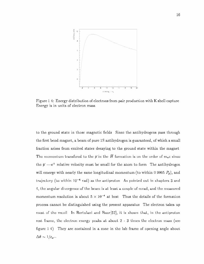
16
Figure 1.4: Energy distribution of electrons from pair production with K shell capture.Energy is in units of electron mass.
to the ground state in those magnetic �elds. Since the antihydrogens pass through
the �rst bend magnet, a beam of pure 1S antihydrogen is guaranteed, of which a small
fraction arises from excited states decaying to the ground state within the magnet.
The momentum transfered to the �p in the �H formation is on the order of mec since
the �p � e+ relative velocity must be small for the atom to form. The antihydrogen
will emerge with nearly the same longitudinal momentum (to within 0.9995 P�p), and
trajectory (to within 10�4 rad) as the antiproton. As pointed out in chapters 3 and
4, the angular divergence of the beam is at least a couple of mrad, and the measured
momentum resolution is about 5 � 10�4 at best. Thus the details of the formation
process cannot be distinguished using the present apparatus. The electron takes up
most of the recoil. In Bertulani and Baur[57], it is shown that, in the antiproton
rest frame, the electron energy peaks at about 2 - 3 times the electron mass (see
�gure 1.4). They are contained in a cone in the lab frame of opening angle about
�� � 1="e� .

17
Figures 1.5, and 1.6 portray the theoretical cross sections calculated by various
authors. The cross section calculations from [47] and [48] agree approximately in
magnitude and as a function of energy. The process, (see �gure 1.2), is insensitive to
the sign of the charge of the projectile; the antiproton could be replaced by a proton
or nucleus of charge Z2, in which case, a factor of Z52 arises. This is because when
the pair production takes place, if the e+ or e� is to have large enough momentum to
be captured by the projectile, it is not strongly a�ected by the target nucleus electric
�eld. After being produced, since the e+ and e� are charged, the nuclear electric
�eld will either attract or repel the particle which, at low energies, would a�ect the
phase space available for binding to the antiproton. When the projectile or target is a
highly charged ion, the nucleus can have a large e�ect on the outgoing lepton moving
the peak energy to larger values because of repulsion. Other calculations have been
done [58],[59], [60],[61] for these nucleus - nucleus collisions with pair production
and electron capture similar to the antihydrogen calculation. They are important
processes to understand they contribute to emittance blowup in relativistic heavy ion
colliders such as RHIC[62],[53].
A calculation of a similar process where a transfer of a negative energy e� in a
continuum state of the target to a positive energy bound state of the projectile has a
di�erent energy dependence than the process described previously[63]. The previous
process can be considered as an excitation of a negative energy e� in a bound state of
the projectile into a positive energy bound state of the same projectile. The energy
dependence is much di�erent because of momentum constraints. The value of the
cross section is similar at higher energies but signi�cantly smaller at the energies of
interest to the experiment. Data exists on high energy pair production and capture
in near collisions of highly-charged ions at a few GeV collision energies [64],[65].

18
Recently, new theoretical calculations were published [57], for the antihydrogen
production cross section which improve on the results of [47], [48], etc. They yield a
smaller cross section which is on the order of 1 pb for momenta near 6 GeV/c. This
is further discussed in chapter 8.

19
Figure 1.5: Theoretical cross section calculations in the range of energies available toE862. \Baur" refers to [48], \BMS" refers to [47], \Eichler" refers to [63].

20
Figure 1.6: Theoretical cross section calculations in a much higher range of energies.\Baur" refers to [48], \BMS" refers to [47], \BB" refers to [40].

21
1.4 The CERN PS210 Experiment at LEAR
In September 1995 at CERN, the PS210 collaboration [5] made a claim of
discovering 9 antihydrogen atoms at CERN's LEAR (Low Energy Antiproton Ring).
Out of approximately 3�105 triggers, the group identi�ed 11 antihydrogen candidates.Their background, mostly from the double charge exchange process, �pp! �nn! �pp,
was predicted to be 2�1 events.
The LEAR antiproton beam momentum (1.94 GeV/c) used in the antihydrogen
experiment is lower than the momenta used at Fermilab . The antihydrogen atoms
were formed in a xenon (Z2 = 2916) clustered gas jet target [66] whereas E862
used hydrogen. The estimated integrated luminosity wasR Ldt = 5 nb�1(�50%)
[5]. The large uncertainty comes primarily from poor knowledge of the jet density.
The antihydrogens produced in the jet travel down the straight section of the LEAR
ring past the interaction point. At the �rst bend magnet, the antiprotons are bent
away. The anti-atoms continue in a straight line until the �rst silicon detector is
encountered where they ionize still within the LEAR vacuum. The ionization products
traverse three silicon detectors, 700�m, 500�m and 700�m thick respectively [5].
Within the �rst two silicon detectors, the 663 keV kinetic energy positron is stopped
and annihilates and a Ee+ + (dE=dx)�p measurement is made. The third detector
measures only (dE=dx)�p. Surrounding the silicon detectors is a 6-fold segmented
NaI(Tl) cylinder. The gamma rays from the annihilation are detected and an attempt
is made to determine whether they are back-to-back. A time of ight measurement
of the antiproton (� = 0:900) is made with 7 scintillation counters and a scintillating
�ber hodoscope. The antiproton momentum is measured with three drift chambers
(8 � 8 cm2) and a dipole bend magnet.

22
The acceptance of the detectors was estimated to be � = 0:3 from Monte Carlo
studies and test measurements. Additional losses from antiproton material interac-
tions and wire chamber e�ciency (not included in simulations) decreases this by a
further 15% [5]. A large uncertainty was due to imprecise knowledge of the inte-
grated luminosity and a rapidly diverging beam. Event selections were made on the
data sample in order to remove mostly single and multi-pion events. The criteria
include requiring the energy deposits in the silicon and in the scintillators to agree
with expectations and a track in the antiproton spectrometer originating from the
interaction. Also required were two NaI hits in wedges in which each had energies in
a band around 511 keV but were not adjacent. No further cuts on the time of ight
or momentum were needed.

23
Sc: Trigger and time-of-flight scintillators, Si: Silicon counters, D: Delay wire chambersNaI : six-fold NaI-calorimeter, H: scintillating fibre hodoscope, B: magnetic dipole field
Experiment PS210 : schematical top view
NaI
BH
D H ScSi
D
ScDSc
D D D H Sc SiScSc
LEAR
2.1m 3.2m
Figure 2a
γ
γ
p0
8040
NaI
Si
NaI
400 600
Si: Silicon counters, NaI : six-fold NaI-calorimeterExperiment PS210 :
Figure 2b
e detecting section +
Figure 2
Figure 1.7: Diagram of PS 210 apparatus [5].

Chapter 2
Antiproton Beam and Target
The apparatus is composed of three parts which are quite distinct because of
their technical functions, the logistics of operating them and their location. The
�rst, the Antiproton Accumulator, is the synchrotron ring at Fermilab where the
antiprotons, created as described below, are stored. The gas jet serves as the target,
and where it crosses the path of the beam, a myriad of high energy interactions take
place. Finally, downstream are the E862 beamlines in which antihydrogen is stripped
and its products guided into the detectors.
The E862 experiment shared the resources of the antiproton circulating beam
and the gas jet target with experiment E835, a charmonium spectroscopy experiment.
The two experiments took data concurrently. Discussion of the goals and impact of
E835 on E862 is found in section 2.3.
2.1 Antiproton Accumulator
2.1.1 Antiproton Production and Cooling
Negative Hydrogen ions (H�) are produced by an electric arc in hydrogen gas
within the electrodes of a Cockroft-Walton electrostatic accelerator, from which they
24

25
KEG Mar 3 , 1995
2 x 2 square foot
Figure 2.1: Placement of E862 equipment in the tunnel, to scale.

26
leave at an energy of 800 keV [67]. The ions are accelerated through the radio fre-
quency Linac up to 200 MeV and injected into the Booster ring operating at 8 GeV.
During injection, they are each stripped into a proton and two electrons by a foil sim-
ilar to the one used to strip antihydrogen, (see section 3.2). The protons are bunched
in the Booster into a batch consisting of 82 rf bunches which are injected into the
Main Ring every 2 seconds, where they eventually reach 120 GeV. While the beam
is in the Main Ring, the rf is used to rotate the longitudinal emittance pro�le of the
beam so that the bunch length becomes 0.7 nsec and the energy spread becomes 185
MeV.
Bunches of 2 �1012 protons at 120 GeV from the main ring impinge on a metal
target made of either copper or tungsten. The antiprotons are produced with a small
time (bunch) structure and small beam diameter matching the protons hitting the
target. The 120 GeV proton beam energy produces a spectrum of antiprotons with
a maximum energy of of 10 GeV[67]. Negatively charged particles are chosen with a
sweeping dipole. Afterwards, a lithium lens with very high instantaneous magnetic
�eld, produced by passing a high current through a rod of lithium metal for a few
�sec, focuses the particles with momentum near 8.85 GeV/c into the injection line.
Antiprotons of 8 GeV kinetic energy are chosen since this is the energy of the booster
and during startup studies, booster protons are used to test accumulator functions.
The 8.85 GeV/c particles injected into the Debuncher ring include muons and pions
formed in the target as well as the antiprotons. While in the Debuncher, the pions
and muons (mostly from decays of the pions) decay within a few thousand turns and
do not get into the Accumulator. The antiproton yield from the target is 7 � 10�7p
per proton. The Debuncher reduces the longitudinal momentum spread from 3% to
about 0.2% through rf manipulations, and the transverse emittance from 20� mm-
mrad to 7� mm-mrad using stochasting cooling. The antiprotons are transferred to
the Accumulator shown with the Debuncher in �gure 2.2.

27
The longitudinal momentum spread of the antiprotons in the Accumulator is
further stochastically cooled to �pp� 2�10�4 and the transverse emittance is reduced
to 2� mm-mrad (area in phase space containing 95% of the beam) corresponding to
a beam diameter of 6.4 mm (4�) at the interaction point. The beam is moved from
the injection orbit to near the core orbit by ramping the radio frequency acceleration
cavities to higher frequency. The beam is then moved onto the core with the stochastic
cooling system over a period of hours, building up what is known as the stack. Beam
currents up to 120 mA are used (1.2 �1012�p) but the beam lifetime decreases when
large intensity stacks are kept and E835's data acquisition (see section 2.3) is swamped
by large trigger rates. Thus most stacks were built up to 80 mA. More detailed
description of the procedures is found in [68].
2.1.2 Deceleration Procedure
The antiproton source rings were designed for a momentum of 8.85 GeV/c. In
order to get to smaller beam momenta, the radio frequency cavities must be ramped
down to the appropriate frequency while simultaneously ramping the magnets accord-
ingly. Part or all of the accumulated beam can be lost during deceleration, especially
during transition crossing, due to instabilities and scraping. Since it takes approxi-
mately 24 hours to build a typical antiproton stack (� 3 mA/hour), deceleration is
a tender procedure and can take as long as 8 hours to perform. After perfecting the
ramp curves during pre-data-run testing, the accelerator personnel used the ramps
nearly automatically. The problem for lower energies is crossing the transition energy
of the machine. At P�p = 5:19 GeV=c, the rf phase of a particular �p with momentum
deviation �p reverses and the beam can be lost since the particles at the front of the
bunch want to trade places with the those at the back at the bunch. A method of
getting around this energy point involves ramping the rf to near the transition point,

28
Figure 2.2: Fermilab Antiproton Source rings showing the transfer lines for stochasticcooling. A50 is the position of the jet target. The beam travels clockwise. (Figurewas adapted from [67].)

29
Figure 2.3: Antiproton density over time vs. orbit position (or energy) showing howstacking builds up the population at the position of the core orbit. Notice the verticalscale is logarithmic. (Figure adapted from [68]).
changing the magnet �elds entirely such as to move the beam onto a di�erent orbit,
and then adjusting the rf to match up with it again. This procedure incurs beam
losses of around 15%.
The rate at which the magnets and rf can be ramped is only about 20 MeV/sec
since the magnets are in saturation at the beginning of the ramps and thus must be
allowed to settle for each step.
2.1.3 Energy Measurement
In order to make use of the �p longitudinal momentum resolution, �pp= 2�10�4,
for rejecting antiprotons, the energy and hence momentum must be measured using
knowledge of the �nal orbit after deceleration. Since the frequency, f, is measured to
better than 10�7, measuring the orbit length, L will determine the value and spread

30
of the beam energy.
� =f � Lc
; E�p =m�pp1� �2
(2.1)
But �L=L is related to the deviation in the velocity:
�f
f=��
�� �L
L=��
�� 2
2t
��
�(2.2)
Since the energy is related to the velocity, the energy spread is:
�E�p
E�p=�2
�
�f
f(2.3)
where the slip factor
� � 1
2� 1
2t(2.4)
represents how close the energy is to the transition point.
The power spectrum (as a function of frequency) is detected by picking up the
Schottky noise from a coaxial �=4 cavity receiver with a natural frequency at 79.323
MHz, the 128th harmonic of the beam revolution frequency, and quality factor, Q
= 305 [69]. The frequency spectrum, (a typical spectrum is shown in �gure 2.4), is
examined with a spectrum analyzer and �t to a Gaussian plus exponential tail. The
Schottky noise spectrum arises because the beam is made up of discrete particles
which have slightly di�erent momenta. Each harmonic of the revolution frequency is
spread out by �f=f .
The orbit length is calculated by measuring the length of a reference orbit at the
momentum corresponding to the 0 charmonium resonance, P�p = 6:23 GeV=c [69].
The reference orbit is measured to 0.7 mm in 474 meters due only to the uncertainty
in the 0 charmonium resonance's mass (see [13] for charmonium data) and that
of the much more accurate frequency measurement. To take into account the fact
that the beam is not exactly on the reference orbit for some energy point, 48 beam
position monitors are examined and compared for the two orbits to get an orbit length
di�erence to an accuracy of 1 mm.

31
Figure 2.4: Typical frequency histogram of the beam at the 128th harmonic.
The value of the slip factor, � = �(E�p), at one energy is determined during
the double scan of the J= resonance by comparing energies and frequencies at the
reference orbit and a \side" orbit[69]. Since dependence of � on energy is known, (see
equation 2.4), it is also a measurement of the transition energy. The measurement of
the energy depends only on very precise frequency measurements and the resonance
masses [69].
The frequency spectrum and various other beam parameters such as beam po-
sitions, beam current, etc. are measured and saved to disk at regular intervals using
the ACNET (accelerator network system). The ACNET system was also used to
save gas jet measurements and to control and monitor E862-speci�c hardware such
as magnet currents, (see section 5.3).

32
2.2 Gas Jet Target
Experiment E862 uses as a production target the E835 hydrogen gas jet. The
jet provides a dense beam of hydrogen molecules with minimal background gas in
the vacuum of the accumulator ring besides the jet itself. We desire to maximize
the number of interactions with a vertex at the origin as compared to the number
taking place away from the jet. The ratio of the number of atoms/cm2 in the jet to
the number of atoms/cm2 in the background gas, the jet target e�ciency or JTE, is
around 90%. If antihydrogen is produced upstream or downstream of the jet, it will
still have the correct trajectory to be detected.
Hydrogen at a temperature of 27 degrees Kelvin, (see �gure 2.6), is injected
into the �rst pressure chamber, J1, (see �gure 2.8)[70]. There are three production
stages (J1,J2,J3) which have successively smaller pressures, the last being close to the
high vacuum of the Accumulator. Entering each new stage, the molecular beam is
collimated by successively larger apertures beginning with a nozzle 37 microns wide
at its thinnest. Since the molecules are very near to the separation line of two phases
(liquid and gas), they easily form clusters of 104 � 106 molecules. At the interaction
point, the transverse jet diameter is 6.3 mm (full width at 10% height) [71]. Across
the beam, the leftover molecules are collected by three recovery stages (R1,R2,R3).
The path in pressure-temperature phase space must be controlled precisely so
as not to condense the gaseous hydrogen (�T = �0:1K;�P = �0:035 bar). On the
other hand, a large range of densities was desired in order to keep the luminosity
constant as the beam current decreases. Nozzle temperature is measured with a
germanium resistance thermometer [72] and read out with a temperature controller.
The pressure at the gas inlet is measured and controlled with similar precision. The
position and angle of the nozzle can be controlled to align the jet through its apertures.

33
Figure 2.5: Hydrogen jet transverse density pro�le 19 mm closer to the nozzle thanthe interaction point [72].
For each store, the jet is left �xed while the beam is aligned with the jet. The average
density of the jet can be found from the ux (molecules/sec) �, the area A, and the
speed V of the clusters (about 600 m/sec depending onpT ):
� = �=(A � V ) (2.5)
Density, cluster speed, and e�ciency, of the jet are calculated from the P-T operating
point and read out over ACNET, (see section 2.1.3). Most of the time, the jet
density was increased automatically as the beam current decreased so that a constant
instantaneous luminosity was used. The density used was in the range 0:5 < � <
2:3� 1014 atoms/cc or an instantaneous luminosity, 1 < L< 4� 1031cm�2sec�1.
The ux of clusters in the jet and the throughput of background gas atoms
pumped in the di�erent chambers are measured easily since they are proportional
to the pumping speed times the pressure and are calibrated with a known hydrogen
gas leak. The jet pro�le is measured with a 0.85 mm needle which moves in an arc

34
Figure 2.6: Thermodynamic phase space of the hydrogen jet's molecules. Dotted linesrepresent the path in phase space taken by the molecules in the jet when di�erentnozzle diameters [72].
through the jet twice. It breaks up the clusters increasing the pressure. The jet is
centered to �0:5 mm. The cluster speed is measured by time of ight using a chopper
and ion gauge separated by 850 mm. The P,T point is chosen to optimize the density
and jet target e�ciency.
When the gas jet is o�, the (1/e) lifetime of the beam is about 400 hours. After
the gas jet is turned on, background gas limits the lifetime to about 30-90 hours
depending on the beam current. Hydrogen is used because the collision energy must
be known well for E835 (see section 2.3). After antihydrogen is created, interactions
with the rest of the jet as it ies through are unlikely since the dissociation cross
section is �diss ' 2:5 � 104 barns or 5:8 � 10�6 interactions/cm for the maximum
jet density used. For an antihydrogen created at the upstream edge of the jet, the
probability of interacting is 3:6 � 10�6.

35
Figure 2.7: Jet-beam intersection.

36
Figure 2.8: Jet target cluster formation, pumps, and chamber dimensions [72].

37
2.3 Charmonium Program
E862 ran as a parasitic experiment to Fermilab E835 the purpose of which was to
map out the charmonium spectrum, speci�cally to take large amounts of data at the
1P1 and �c resonances and to make an exhaustive search for the �0c resonance as well
as measurements of the �1, �2, J= , and 0 resonances. The amount of luminosity
accumulated at each center of mass energy point was aligned to E835's need to make
precision measurements of these states. Most of the data are at a momentum around
6 GeV/c. The E835 apparatus downstream of the jet target include central tracking
(scintillating �bers and silicon barrel), scintillating hodoscopes, Cerenkov counter, a
cylindrical, lead-glass electromagnetic calorimeter and a forward calorimeter extend-
ing roughly 10 feet from the jet. A luminosity monitor near the jet is described next.
More information can be found in [69] and [73].

38
Figure 2.9: Charmonium spectrum

39
2.4 Luminosity
Although the density of the jet is fairly well known and the intensity of the
�p beam is known, the luminosity calculated this way is only accurate to about 10%
since the cross sectional areas of the crossing jet and beam are not known well enough.
Fortunately the luminosity monitor [74] for E835 can count the recoil protons from
the forward elastic scattering region. The number of recoil protons, S, is related to
the integrated luminosity but depends on the solid angle subtended and di�erential
elastic scattering cross section at the detector position (t = four momentum transfer).
ZLdt = S=(
Zd�
dd) ' S=( <
d�
dt
dt
d>) (2.6)
since the cross section is nearly independent of position across the detector (to <
0.1%). This device is an ion-implanted, solid state, silicon detector and is used to
count recoil protons at 3:5� forward from the vertical, (see �gure 2.10). The de-
tector is located 147 cm below the interaction point. A histogram in energy de-
posit corresponding to a range of momentum transfers t, 0:0075 (GeV=c)2 < t <
0:0108 (GeV=c)2, (shown in �gure 2.11), is read out using a histogramming ADC.
The spectrum is �t to a proton recoil peak plus a smoothly falling background cross
section. The number of events in the recoil peak are extracted from the �t compared
to the known elastic di�erential cross section in equation 2.6 to determineR Ldt. The
detector area was calibrated with an 241Am whose activity was measured to within
>1% [74]. The energy scale was calibrated with a 244Cm source with two alpha emit-
ting lines separated by 42 keV. The integrated luminosity is measured with a 4%
systematic error. The error arises from imprecise knowledge of the active area, and
thus subtended solid angle (2%), and from the uncertainty in the known cross section
(2%). More detail is available in reference [74].

40
Figure 2.10: E835 luminosity monitor angle de�nition [74].
Figure 2.11: E835 luminosity monitor spectrum - for �p momentum = 5974.4 GeV/c

41
Figure 2.12: Theoretically expected antihydrogen production rate over range of mo-menta available. Also shown is the integrated luminosity taken by the experiment toshow at which momenta the data was concentrated.

Chapter 3
The E862 Positron Spectrometer
3.1 E862 Detectors
Antihydrogen atoms are created within the < 1 cm3 interaction region where the
antiproton beam and hydrogen gas jet target intersect, (see �gure 2.7). Downstream,
after a long straight section, the �rst dipole magnet, (see �gure 3.1), bends the an-
tiprotons by 5o as part of their trajectory around the Accumulator ring. Within the
magnet, a Y-shaped vacuum pipe was installed so that the neutral antihydrogen (un-
a�ected by the magnetic �eld) can continue on straight within high vacuum (10�11
Torr).
At a distance of 24.366 meters past the jet, a thin carbon foil ionizes the anti-
atoms. The velocities of the positron and antiproton are almost equal. The direction
of the antiproton coincides with that of the antihydrogen. The positron is signi�-
cantly multiple scattered in the foil and enters a magnetic spectrometer, consisting
of solenoids for focusing the cone of positrons and a dipole which bends them by 40o
out of the path of the antiprotons. The spectrometer beampipe is under high vacuum
and ends in a plastic scintillator plug. The positron stops and annihilates in the plug,
whence the resulting back to back gamma rays are detected by a surrounding NaI(Tl)
cylinder.
42

43
The antiprotons are hardly bent by the �rst solenoid and dipole and continue
down a beamline in partial vacuum. They are bent by two larger dipoles 40 feet
downstream by a total of 10�. Three proportional wire chambers are placed upstream,
downstream, and in between these magnets so that a momentummeasurement can be
made. There are also time-of- ight counters at the beginning and end of this stretch
after the positron is bent away.
Stripping Foil
Solenoid
Solenoid
NaI halves
e+ scintillator
40 deg. Dipole
e+
5 deg. Dipole
ToF#2
PWC#3
PWC#2
PWC#1
5 deg. Dipole
5 deg. Dipole
ToF#1
Gas Jet
PositronSpectrometer
AntiprotonSpectrometer
_p
_H
_p
~20 m
~2 m
~10 m
~10 m
AntiprotonAccumulator
Figure 3.1: Schematic of E862 beamline elements.

44
Table 3.1: Ionization rates and mean decay lengths for antihydrogen atomsState �p Momentum A5B3 B-�eld Ionization Mean decay
(GeV/c) (Tesla) rate (sec�1) length (cm)States are , in order: 1000,2100,2010,2001
2100 3.5 0.7 8:3� 10�6 3:6� 1015
2001 3.5 0.7 1:4� 10�4 2:1� 1014
2010 3.5 0.7 2:4� 10�3 1:3� 1013
1000 5.7 1.1 2:2� 10�55 1:4� 1066
2100 5.7 1.1 6:9 � 109 4:42001 5.7 1.1 4:4� 1010 0:682010 5.7 1.1 2:8� 1011 0:111000 8.9 1.7 5:0� 10�12 5:9� 1021
2100 8.9 1.7 8:3� 1014 3:6� 10�5
2001 8.9 1.7 2:2� 1015 1:4� 10�5
2010 8.9 1.7 5:7� 1015 5:2� 10�6
Although the antihydrogen atoms are electrically neutral, getting through the
large magnetic �eld of the bend dipole, A5B3, is non-trivial. Most of the atoms
are formed in the ground state. About 10% can be formed in excited states since
the production depends on the principal quantum number roughly as � � 1=n3[40].
Because the atoms are traveling at relativistic speeds, the magnetic �eld will be
transformed into an electric �eld as viewed in the antihydrogen rest frame. This
will cause a change in the energy levels due to the Stark e�ect and will increase the
probability that the e+ will ionize (by tunnelling out of the potential well). Within
our energy range, the ground state is una�ected. The excited states have enormously
higher ionization rates. Table 3.1 illustrates how 1S atoms are not a�ected but n
= 2 atoms are mostly ionized in A5B3. The notation for n = 2 states comes from
expressing the hydrogen hamiltonian in parabolic coordinates which are described
along with the ionization rate calculation in section B.4.

45
3.2 Foil Stripper
The antihydrogen atoms travel down 80 feet from the gas jet in high vacuum.
Connected by a bellows there is attached a vacuum enclosure which holds a 1/32"
thick aluminumwheel. The wheel has 6 circular cutouts, symmetrically placed, which
contain 3 stripper foils, 2 radioactive sources, and a 1" hole so that any particle could
pass through, (see �gure 3.4). A carbon foil about 440 �g=cm2 thick (1 �m) stripped
the anti-atoms into �pe+ with 99% e�ciency. The other foils were a spare 440 �g=cm2
and a 777 �g=cm2 or (1.8 �m) thick foil. The probability of stripping a high energy
�H with the 777 �g=cm2 was 100%. The probability of other neutrals converting in
the foil and yielding a positron is small. The foil thicknesses are determined by the
manufacturer by weighing the foil and dividing by the area. Carbon is used for its
ease in manufacture and resistance to thermal load (from beam heating).
The cross section, �(E) for stripping the ground state as a function of energy
[75], is displayed in �gure 3.2:
�(E) = �ion + �exc =4�a2o�2
(Z�)2[ln(� =�)2
0:16� �2] (3.1)
which decreases exponentially with energy until a few hundred MeV and then de-
creases much more slowly. The cross section for excitation is about twice as large as
the direct 1S ionization but excited states strip in the foil much more easily so the
e�ective stripping cross section is as shown.
The stripping probabilities are calculated using measurements of single and
double ionization of negative hydrogen (H�) ion beams [79],[76] (800 MeV), and
[80],[77],[78] (200 MeV). Stripping the ions with foils is used as a charge exchange
injection mechanism for storage rings. These foils were used to strip H� ions incident
from the Linac at injection to the Fermilab Booster ring (200 MeV) (see section 2.1.1).
A system of equations predicts the fraction of hydrogen in each charge state given

46
Figure 3.2: Cross section for stripping H0 (cm2). Measurements from [76],[77],[78].
the charge exchange cross sections [77]:
dN�
dx= �(��10 + ��11)N
� (3.2)
dN0
dx= ��10N
� � �01N0 (3.3)
dN+
dx= ��11N
� + �01N0 (3.4)
The solutions for the fraction in each state as a function of the foil thickness, x, are:
N� = e�(��10+��11)x (3.5)
N0 =��10
��10 + ��11 � �01
he��01x � e�(��10+��11)x
i(3.6)
N+ = 1�N� �N0 (3.7)
The fractions were measured experimentally for various foil thicknesses in the
range 10 < x < 300�g/cm2. They were �t to the expected fractions using the cross
sections as parameters yielding cross sections at 200 MeV [77].

47
Figure 3.3: E�ciency for stripping H0 as a function of carbon foil thickness. Thesolid curve is for a 3 GeV/c antihydrogen, the dashed for 6 GeV/c, the dotted for 9GeV/c.
Figure 3.3 shows the stripping e�ciency of carbon for hydrogen incident ener-
gies of 3 GeV, 6 GeV, and 9 GeV as a function of thickness of a set of foils. The
e�ciency at these higher energies for stripping antihydrogen was calculated by lin-
early extrapolating the data. This included the highest energy cross section data at
800 MeV as a worst case scenario and did not include the relativistic increase of the
cross section expected in the higher energy range. The � 440�g/cm2 thickness was
chosen to give > 99% e�ciency.
In the case of E862, we assume that the antihydrogen has the same stripping
cross section as hydrogen in the carbon foil. It is also assumed that the hydrogen
atoms (H0) formed by charge exchange in [77] were in the ground state. The stripping
cross section for excited state hydrogen atoms will be slightly larger anyway.

48
Figure 3.4: Vacuum box for target wheel.
3.3 Radioactive Sources
One of the radioactive sources mounted on the wheel was 207Bi, a monoenergetic
electron source with an initial activity of 10�Ci. It was used to �nd the correct
magnetic �elds for focusing the positrons. A �+ source, 68Ge with an initial activity
of 10�Ci, was used to check the integrity of the path all the way through to the sodium
iodide. Since the �+ spectrum has an energy endpoint of about 1.899 MeV [13], the
magnets had to be tuned below any �eld used for normal data-taking. The 68Ge
source was constructed of evaporated metallic salt of germanium contained within a
Nickel ring with 0.0002" nickel cover plates. The active area was 0.713 cm2.

49
Table 3.2: Antiproton beam parameters using Fermilab standard emittance de�ni-tions. The emittance used in both dimensions is 2� mm-mrad, the maximum mea-sured.
�xq�x�x=6� 1.57 mm
��xq�x(1 + �2x)=6��x 0.21 mrad
�yq�y�y=6� 1.40 mm
��yq�y(1 + �2y)=6��y 0.24 mrad
3.4 Antihydrogen Beam Parameters
It was essential to know how large the beam spot would be on the foil target
and the positron scintillator, and how many wires would be needed in the chambers.
Above all, knowing the antihydrogen would not hit the beampipe anywhere was of
utmost importance.
The beam size distributions are characterized by the standard deviations found
in table 3.4. These numbers assume both transverse emittances are equal to 2� mm-
mrad, an upper bound on their maximum value. The emittance in the x dimension,
�x is given as the area of the phase space (x; �x = px=pz) containing 95% of the
particles. The y emittance is de�ned similarly. The Courant-Snyder parameters,
� = 0 and � are calculated from a knowledge of the lattice (�eld strengths, positions
of the magnets around the ring) [81]. The beam has a roughly circular cross section
(equal width Gaussian distributions in x and y) with large coupling between the two
transverse dimensions.
"x = �2��2x=�x � ln(1 � F ) = 6��2x=�x (3.8)
[81] where F is the fraction of particles inside the phase space ellipse (95%). The
angular spread is:
��x = �x=�x (3.9)

50
The beam emittance in the accumulator ring was usually less than 2� mm-mrad.
E862 has measured the emittance by examining the high momentum tracks which
enter the E862 antiproton spectrometer. Section 6.6.4 discusses these measurements.
The antihydrogen candidates' tracks clearly form a transverse emittance envelope
corresponding to �x; �y < 2� mm-mrad. This data took the whole running period
to accumulate, so it does not serve as a method of monitoring the emittance during
the run. The transverse emittances are usually extracted from a measurement of the
betatron cooling sideband spectrum of the beam. The angular divergences, ��, are
calculated using the beam spot size and beta function at that position of the ring.
The position of the beam centroid is measured by beam position monitors.
The beam position monitors are basically semicylindrical pickup electrodes
within the vacuum pipe installed between the pole faces of the quadrupole magnets.
There are 48 monitors in each dimension; not all quadrupoles have a monitor. They
are tuned to a harmonic of the beam revolution frequency and must have the beam
partially bunched in order to receive a signal. The horizontal and vertical beam posi-
tions measured by the monitors installed in the two accumulator quadrupoles, A4Q1
and A5Q1, just upstream and downstream of the jet, were used to draw a line to
the foil target. The neutral antihydrogen follows a straight path from the interaction
point collinear to the beam at that point. The monitors achieved a precision of �1mm in both transverse dimensions. If the maximum error was encountered in the
two monitors nearest the jet target, a beam steering error of 0.35 cm would result at
the �rst downstream bend magnet, A5B3, where the �H0 exits the storage ring. This
is at least 4 times smaller than what would result in scraping by the beam pipe in
the A5B3. During the calibration run, (see section 4.3), the beam centered in both
quadrupoles was also seen to traverse a centered path through the wire chambers.

51
At the position of the E835 jet target interaction point, the �p beam is within
a zero dispersion region such that a spread in momentum will not translate into a
spread in position. Section 6.6.4 shows that the phase ellipse de�ning the emittance
is not aligned along the x and x0 axes. This is due to a cross term, � = �12d�ds
in the
expression for emittance[81]:
�
�= x2 + 2�xx0 + �x0
2 (3.10)
The beta function, �, is dependent on magnet con�gurations and �elds only, and s is
the path length of a particle.
The momentum transfer during the production is small, �px=p � 0:181=3000 =
0:06 mrad making ��x larger byp0:22 + 0:062 = 0:21 mrad. At the position of the
foil target, the beam size at one standard deviation in x and y is �x = 0:53 cm
and �y = 0:67 cm on average but depends on the emittance. If a circular beam is
assumed, with �r = 0:6 cm, the beam covers 22% of the foil at 1�. Given the (nearly)
Gaussian probability distribution for a hit outside the radius r, P = e�r2=2�2, 90% of
the beam is contained within a disk of diameter 1" = 2.54 cm for a beam centered on
the foil. Section 7.4.1 discusses ine�ciencies incurred when the beam is not centered
on the foil. The A5B3 beampipe was speci�cally redesigned to accomodate 3� of
the straight- ying antihydrogen beam in both the vertical and horizontal directions.
Discussion of the beam spots measured during the calibration run can be found in
section 4.3. The beam size was measured in March 1997 using the ying wire system
above the transition energy and matched expectations based on an emittance of 1.6�
mm-mrad in both dimensions and a �� < 0.25 mrad angular spread at the gas jet.

52
Figure 3.5: Flying wire pro�les of antiproton beam at A3Q7 and A4Q14, respectively.
3.5 Positron Magnets
3.5.1 Design and Simulations
The positrons multiple scatter in the 440�g=cm2 (10�3 radiation lengths) foil
enough to exit within a � = 6� cone (3��) at 1.2 MeV. It is important to remember
that the \beam" E862 uses is a very low rate source of antihydrogens. Subtle beam
e�ects like space charge are not applicable since more than one positron is never
within the spectrometer at any one time. It was desired to bend the positrons out
of the way in order to detect them. This would also entail reproducing a reasonable
beam spot on the �nal detector to ensure the hit was not from background. A small
bend dipole is adequate for the application, but because the beam has an angular
divergence, it is better if the dipole is able to focus positrons entering at di�erent
angles so they will converge at the exit point.

53
Figure 3.6: Schematic of E862 beamline elements.

54
Figure 3.7: 40o dipole for positrons showing anged edges at 10�.
Dipole Focusing
We can characterize a sector dipole as a thin lens located at the center of the
dipole. The focal length in the bend plane is equal to the ratio of the radius of
curvature to the tangent of the bend angle � = 40o, fh = rg=tan�. The radius
of curvature is rg = p=(eB) where p is the momentum and e is the charge of the
electron. One problem is that there is focusing in the plane of the bend but not in
the normal plane. In the case of E862, the bend plane is the horizontal and the normal
plane is vertical. A sector dipole having anged edges has fringe �elds that particles
encounter so that vertical focusing (or defocusing) occurs. Each of the two edges can
be characterized by a certain focal length, fv = rg=tan� where � is the angle between
the edge of the magnet and the central particle trajectory. When � = �4= 10o, the
overall focal lengths of the magnet in x and y are best matched. Field plates are
positioned at the entrance region to minimize the extent of the dipole fringe �eld.

55
Figure 3.8: Diagram of entrance/exit angles of e+ for 40o bend dipole.
Figure 3.9: Focusing solenoid for positrons. The magnet is perfectly cylindrical. The atness at the right edge is an artifact of a scan.

56
Solenoid Focusing
Solenoids were chosen to collect the distribution of positrons exiting at large
angles. Since the solenoids are symmetric about the beam axis, they are easier to
construct accurately, but the focusing power of solenoids gets much worse for higher
energy beams. They are often used in electron microscopes, for example, since the
electron energy is relatively low. The three magnets form a symmetric, point to
point focusing system. Two solutions exist which depend on the magnetic �eld in
the solenoids. The trajectories can either cross each other at a node in the center
of the dipole or not. The higher magnetic �eld solution causes the crossing to take
place and has a higher acceptance, �7% for o�-momentum positrons. The lower �eld
solution has a �3.6% longitudinal momentum acceptance window.
The Lorentz force on the positron while its radial position is increasing within
the solenoid is in a � direction, � being the azimuthal angle around the solenoid axis.
The e+ gains a momentum component in the � direction. This leads to a component
of the force in the negative radial direction which is focusing. When the net radial
component of the e+ momentum is negative (around the middle of the magnet), the
force component in the � direction changes sign. If the �eld is reversed, there is no
di�erence in the focal length because the e+ receives the same changes in the radial
components even though the � motion is reversed. This di�erence in the � motion
is responsible for the two solenoids producing beam spots at their image plane which
have di�erent locations. This is due to the di�erent image rotations imparted by the
solenoids. If the solenoids both have a length such that both images rotate by n�
then the images have the same position in the image plane. After testing, it was
discovered that misalignments necessitated the polarity switch in order to reverse the
rotation of the image and thus move the beam spot. Basically, if the e+ propagates

57
y (cm)
-2 -1 0 1 2
z (cm)
y (cm)
050
100150
-2 -1 0 1 2
y (cm)
-2 -1 0 1 2
z (cm)
y (cm)
050
100150
-2 -1 0 1 2
Figure3.10:Positrontracks(simulatedwithTransport)atnominalmagnetic�eld.
Figure3.11:Positrontracks(simulated)with�rstsolenoidturnedo�.Dipoleisnotonineithersimulation.
alongthesymmetryaxisofthesolenoid(x=y=0),itexperiencesnokick.More
detailaboutdipoleandsolenoidfocusingcanbefoundin[83]and[82].
3.5.2ConstructionofMagnets
ThemagnetswereconstructedatCaliforniaMagneticsduring1995.Atthe
factory,oncetheframeswereformed,themagnetswerewound.Thesolenoidhas
fourlayersofsquarecrosssection(0.1875"x0.1875")cable,eachwoundintoahelix
of48loops.Therewere(0.125"x0.125")squareholesinsidethecableforthecooling
water ow.Eachpoleofthedipolewaswoundwith6layersof8loopsofsquare
(0.1875"x0.1875")cable.Thewaterholesforthedipolewere(0.1"x0.1").After

58
Figure 3.12: Nonlinearity of solenoid, dipole magnetic �elds with applied current. The�elds vs currents for di�erent currents were �t to a straight line. The di�erence of themeasured magnetic �elds from the �t are displayed as percentages. The dependenceis nearly linear at higher current but exhibits some deviation at low currents.
winding, a thin layer each of (2 mil) of Kapton Polyamide �lm, \B" Stage epoxy-�lled
tape, Nomex Type 410 Class R tape, and P-21 black tape was glued over the cables
for protection from the oxidation, etc.
3.5.3 Magnetic Field Properties
When the magnets arrived at Fermilab, initial testing was done. The solenoids
perform linearly throughout their range of current up to 160 Amps. The dipole was
found to have a signi�cant (3%) hysteresis e�ect when the polarity of the current (and
hence B-�eld) was switched. In order to track the dipole's B-�eld, a Hall probe was
placed inside the dipole. The dipole has to be cycled a few times in order to bring
the magnets to a reproducible �eld setting within 0.5%. It was originally thought
that the solenoids would not need their polarity switched to observe electrons while
the dipole needed to be �eld reversed.

59
The Hall probe is a solid state detector, 1" x 1" in area. The probe is glued
to the bottom pole of the dipole magnet and held down by an aluminum bracket
to keep it normal to the �eld and prevent the cables from applying torque to the
probe. Temperature compensation is included at the detector. The analog level is
sent to the counting room over 30 feet of cable and digitized. The device measures the
magnetic �eld to a precision of 0.01 gauss, roughly 10�4 of the �eld value. However,
the resolution is limited to �0:5 gauss. When the magnets were turned o� and/or
were �eld reversed, there is a remnant �eld measured at less than 10 gauss. The
dipole was always set by adjusting the current to get the correct �eld.
3.5.4 Beam Test Apparatus
� Table ConstructionA non-magnetic (aluminum) table was constructed to support the spectrometer
elements. The table height was such that the beampipes were at the same height
as the beam (28.5"). The top part of the table was a 1/2" plate attached to
girders. This slid on Te on pads (for easy horizontal positioning) attached to
the bottom part, which was a 3 point truss to allow easy vertical positioning.
Screw adjustments provided easy translational and rotational motion of the
table in the horizontal plane to submillimeter precision.
� Alignment Blocks raised the elements such that the vertical positions of the
center of the vacuum pipe, the source point, and the center of the magnets lined
up. After testing, the solenoids had to be repositioned to move the beam back
to the center of the beampipe when it was found to be partially hitting the
wall. Moving the solenoids by equal distances in the same or opposite direction
in the transverse plane allowed changing the beam position in those directions
independently for the two di�erent solenoid tunes.

60
� Vacuum After installation the vacuum was brought down to 10�5 Torr with a
roughing pump and turbomolecular pump. The system was leak checked with
a standard Helium leak (�xed leak rate). The vacuum pipe was tested down to
10�6 Torr with a leak rate of 4�10�8 cc/sec. When attached to the accumulator
vacuum in the AP50 tunnel, the vacuum reached 10�7 Torr.
� Water cooling Since the maximumsolenoid current generated substantial heat
(1 kW), two water cooling circuits were designed into each of the 3 magnets
(dipole had 1 per pole). During electron source testing, a deionized water system
was setup, (see �gure 3.13). The temperature was kept constant at 80o F with
a small ow rate (max 20 gpm at 120 psi). In operation, each magnet circuit
took less than 1 gpm with 50 psi pressure drop. Two trip circuits (bimetallic
switches) were attached to each of the magnets so that if the coil temperature
rose above a threshold, the appropriate power supply would be turned o�. In
the tunnel, the cooling came from the Low Conductivity Water (LCW) water
circuits already cooling the large ring magnets. The trip circuitry was the same.
3.5.5 Monoenergetic Electron Source Testing
To test the focusing at one energy, a bismuth-207 (207Bi) radioactive source with
an activity of 10�Ci (3.7 �105 Hz) was used. The source is deposited on a 1" diameter
nickel substrate. An aluminum holder held the disk and was attached to the target
wheel. The 207Bi source was actually about 1 mm in size and covered with a coating
which slightly a�ects the energy and the angle of the e� as it leaves the source. The
fact that the line energies [13], Ee� = 0.975 MeV, 1.07 MeV, were well below the
range expected in the antihydrogen data, 2 < Ee+ < 4:5 MeV, meant that using the
test data would require some assumptions about how the focusing would scale with

61
Figure 3.13: Deionized water system in Lab 6.
the energies. The two lines are 7% and 2% of the rate respectively [13]. Still, the
need to accurately image a beam spot at any energy and the ability to resolve the
two closely spaced peaks made the test data important. The beampipe at the center
of the solenoid was 1.5" in radius. This meant the fractional acceptance was about
3:6 � 10�3 and the expected rate was 220 Hz. The best rates measured were about
50 Hz with no collimation.
Table 3.3: Magnetic �eld settings vs. beam energyp�p Ecm;�pp pe+ Bdip Bsol;1st Bsol;2nd
(GeV/c) (MeV) (MeV/c) (Gauss) (Gauss) (Gauss)2.562 1.395 135 288 4613.71 2.99 2.021 195 417 6674.068 3.097 2.216 214 457 7315.615 3.527 3.058 296 631 10095.97 3.619 3.25 314 671 10736.233 3.686 3.395 328 701 11218.9 4.30 4.847 469 1000 1600

62
Figure 3.14: Measured magnetic �eld of solenoid along axis.

63
Figure 3.15: Testing the spectrometer with the bismuth source in Lab 6. Count ratescans over the dipole applied current.
Figure 3.16: Testing the spectrometer with the bismuth source in Lab 6. Count ratescans over the solenoid applied current.

64
To detect all the electrons possible at the end, a 2" x 2" x 1/2" plastic scintillator
square was directly mounted to a phototube and brass apertures used to collimate
the beam selectively at either end. The signals for electrons with the phototube
set at -1800 V were about 500 mV maximum amplitude and could be distinguished
clearly from gamma ray hits and MIP hits with much higher (2-3 V) amplitudes. The
electron signal rate changed consistently when the acceptance of the spectrometer was
changed. The signals were discriminated at two di�erent thresholds of 300 mV and
1 V and counted. The rates were compared, the latter being used as the background
rate since most background was from high energy particles. The background rate
was checked by placing a >1/4" aluminum plate 6" x 6" before the scintillator and
measuring the rate. This background rate was subtracted from the electron hit rate.
Shown in �gure 3.14 is the measured Bz pro�le along z in the solenoid. The
plot demonstrates the symmetry of the �eld along the central symmetry, z, axis
of the solenoid. The next two �gures, (3.15, and 3.16) are the results of scanning
the DC currents of the magnets over a certain range corresponding to the bismuth
source energy. Figures 3.17, and 3.18 were scans nearly identical to the previous two
but done after �nal alignment in the tunnel. The solenoid is set to a value found
by simulation to give good focusing for 0.975 MeV kinetic energy electrons and the
dipole scanned over a 20% range in current. The peak corresponding to the 0.975
MeV electron line is visible. The smaller bump at the right corresponds to the electron
line at 1.047 MeV. The dipole current was held �xed at the peak and the solenoid
current ramped to investigate focusing. Although the magnetic �eld needed to focus
is linearly dependent on applied current, it is not as easy to predict the e�ect of
changing the solenoid currents as it is for changing the bend angle. The large peak
to the right corresponds to the low dispersion solution where the electrons cross the
central trajectory at the symmetry point in the dipole. This solution would obviously

65
have better collection e�ciency. A peak for the high dispersion solution is harder to
see at lower solenoid current.

66
Figure 3.17: Scan over the dipole �eld for 207Bi after �nal setup in tunnel.
Figure 3.18: Scan over the solenoid current for 207Bi after �nal setup in tunnel.

67
Plot 3.19 shows the e�ect on the electron rate of moving the source out of
the plane of the beamline by rotating the wheel. The source position dependence
gives a feel for the acceptance of the system. Speci�cally, scans were done with
the electron line source to see how far away the beam could be without missing
the positron spectrometer. The limiting factor seems to be the size of the T-shaped
beampipe section leading up to the e+ scintillator (1") as projected back to the source
plane. This projection is not the same for the two tunes. As seen in �gure 3.19, the
distribution for the high dispersion tune shows an o�set of about 4.5 mm above the
focusing plane whereas the low dispersion tune does not show any noticeable o�set.
During alignment studies, the �rst solenoid was o�set by 3/16" vertically in order
to center the beam on the scintillator which lies in the image plane. Because of
symmetry, the second solenoid was moved -3/16". Thus, it was thought the electrons
might be seeing a magnetic aperture (a signi�cant deviation of the �eld from its
required value for this momentum) although the solenoid has a nearly constant �eld
across most of its inner diameter.
The spectrometer has a slightly di�erent focusing plane for the two tunes. The
high dispersion tune focuses positrons in a plane rotated about 45o with respect to
the horizontal so that the o�set in the object plane results as evidenced in �gure 3.19.
The object plane is the plane containing the source.
3.6 Positron Detectors
The purpose of the positron counter, a plastic scintillator, was to detect the
positron, measure its arrival time precisely enough to trigger, and insure its annihila-
tion with an electron. The annihilation yielded back-to-back gamma rays which are
detected by sodium iodide, NaI(Tl) cylinder halves, (see �gure 3.21). The gamma

68
Figure 3.19: Vertical position scan, for high and low dispersion tunes
ray energy and arrival time as well as positron energy (from the plastic scintillator)
were measured as well.
3.6.1 Positron Counter
A plastic scintillator plug 1" in diameter and 1" thick served as the end plug for
the high-vacuum as well as stopping the e+ and annihilating it. The half inside the
beam pipe was actually only 0.9" in diameter. When a positron enters the scintillator,
one of several things can happen. It can back scatter. It can lose all its energy to the
scintillator through ionizations and annihilate before exiting, which it will do 99% of
the time if it goes straight into the scintillator. It can cut the corner of the scintillator
and annihilate in the sodium iodide or the aluminum inner case. Finally, if it is close
to the edge, it can be scattered into the sodium iodide as opposed to having a straight
path crossing into it; in this case, it most likely would annihilate in the aluminum 1"
tube. The �rst possibility is small and the probability depends on the energy of the
positron. Monte Carlo calculations using EGS and GEANT showed the fraction of

69
Table 3.4: Probability e+ will back scatter from the plastic scintillatore+ Energy Probability2 MeV 0.011 (90%)3.5 MeV 0.008 (90%)
the time it is back-scattered completely out of the scintillator (see table 3.6.1). The
remaining possibilities, though, depend on how collimated, focused, and centered the
\beam" of positrons is. If the positron annihilates outside the plastic scintillator, the
gamma rays can both deposit energy in the one half. If one is scattered, it can leave
part of its energy in one half and part in the other half. We have no way of resolving
these annihilations by observing the two photon opening angle. The energy deposit
in each half may fall above the 511 MeV ��E energy window. The total energy
should be 1022 MeV, though, unless the e+ annihilates in ight.
Most positrons come to rest before annihilating. However, the positron can
annihilate while in ight, which alters the gamma ray energies. The cross section per
electron as a function of = Ee+=me is [84]:
�annih = �r2o1
+ 1[ 2 + 4 + 1
2 � 1ln( +
q 2 � 1)� + 3p
2 � 1] (3.11)
The probability of annihilating in ight at a certain energy can be calculated by
dividing the cross section for annihilation, which is a function of energy, by the
energy loss per unit distance for that material [85],[86] and then integrating up to the
incoming energy. The material density is denoted as N (atoms/cm3). The energy loss
per distance ionizations for high energy electrons is [85] (I � 15 eV, ro = 2:8� 10�15
m):
�dEdx
= NZ2�r2ome
0@ Eq
E2 �m2e
1A2 "
ln�(E �me)(E
2 �m2e)=2meI
2Z2�+�me
E
�2#
(3.12)

70
If the material is thick enough to stop the positrons, the probability of annihilation
in ight per e+ is, (also shown in �gure 3.20):
Pin�flight = �ZNZ Ei
me
�(E)dE
dE=dx(3.13)
Otherwise, the lower limit of integration is replaced by a cuto� energy Ec which
depends on the thickness and the probability of annihilating at rest is not equal to 1,
Pat�rest = exp(�ZN
�
dE=dx
!jEc) (3.14)
The annihilation cross section has a local maximum at 511 keV kinetic energy (E = 1
MeV) and then drops o� at higher energies. The percentage of annihilation in ight
is between 5 and 10% for plastic scintillator. The e�ective Z for polyvinyltolulene
used in plastic scintillator (monomer 2� CH3C6H4CH = CH2) is Z = 1.1.
The scintillator was coupled with optic epoxy directly to a 1" photomultiplier
tube since the hole in the NaI was only 1 1/2" in diameter. The phototube was chosen
for speed as well as size, having an intrinsic risetime of 2 nsec, since it is an intrinsic
part of the trigger. The base had 10 stages. The spread of the time of arrival of
the pulse for a particular positron energy was about 500 psec. Of course, the trigger
timing was less crucial than the time of ight measurement, and the transit time
spread in the focusing system was considerable. The scintillator pulse was typically
20 nsec wide. It was split, discriminated at the -100 mV level and the logic pulse
digitized in 4096 25 psec bins. The analog pulse was digitized in a charge integrating
ADC in 2048 0.25 pC bins using a gate width of 200 nsec.
3.6.2 Sodium Iodide(Tl) Gamma Ray Detector
After the e+ loses most if not all of its kinetic energy in the scintillator, it
annihilates and two essentially back to back photons are detected by the two halves

71
Figure 3.20: Probability for an e+ annihilation in ight as a function of e+ totalenergy. The peak at 1.022 MeV total energy is clearly shown in the di�erentialprobability distribution.

72
of a sodium iodide cylinder 7" in diameter surrounding the scintillator. The sodium
iodide, being hygroscopic, is completely contained within an aluminum can 1/16"
thick with 6 holes on the top side for phototubes glued directly to the NaI. The
bore in the middle is lined with aluminum as well and this bore represents a loss
of acceptance for a single photon of 1.86%. The aluminum lining of the at faces
separating the halves represents a loss of geometrical acceptance of 1.14% again for
a single photon. When the annihilation gammas enter the sodium iodide, they get
Compton scattered by electrons. Thus the energy window had to be wide enough to
accept hits in which one of the annihilation gammas Compton scattered.
The phototubes and bases were adjusted for overall gain matching of each triplet.
This facilitates summing the analog pulses and reading out only 2 analog signals but
retains the safety factor of allowing one to fail while still recording 70% of the half's
energy on average. A looser cut on photon energy would still reject events not having
2 hits. The analog pulses after 550 nsec of cable were read into a 1 �sec gate width
charge-integrating ADC. Typical energy resolution expected of sodium iodide is 8-
10% for photon energies on the order of 1 MeV[87]. A copy of the analog signal
was ampli�ed by 10X and discriminated at -400 mV corresponding to about 250 keV
photons. The signal's arrival time was digitized in 2048 50 psec bins.
The high voltages were set as high as possible on the plateau curves, (see �gure
3.22), without inducing a large amount of noise on the signals. The gains of the
PMTs were adjusted at the factory to be equal, but the phototube bases were not
adjusted. Each base had two screw adjusts, one for the focus and one strictly for the
gain. Both were adjusted so all the signals were about equal (to 5%) at the same
applied voltage. The voltage level was then set at 1300 V. The operating range is
900 to 1400 V but the e�ciency is very low below 1300 V because of high threshold.

73
Outer Case
NaI
Plastic Scintilator
PMT
5.87cm
3.39cm
19.7cm
2.88cm
Figure 3.21: Diagram of sodium iodide detector
The pileup makes the signals very noisy above 1350 V. The source used for testing,
(Cs137), had a higher rate than the expected data rate for beam running (>1 kHz).
3.6.3 Positron Source Testing
The 68Ge source has a positron beta spectrum, (see �gure 3.23), as well as a
discrete spectrum of gamma rays resulting from nuclear transitions. This source was
used to verify that the e+ counter signals were timed relative to the NaI(Tl) detector
and to see that the gain of the NaI phototubes did not shift, by observing the position
of the annihilation peaks. Typical �ts of the ADC distributions to gaussian shapes
(energy resolution determination) are shown in �gure 3.24. As seen in �gure 3.25, the
e+ ADC count depends on the current as the dipole and solenoid currents are changed
together for the high dispersion tune. This was done to cut slices in momentum
through the �+ spectrum. Figure 3.26 shows a similar dependence of the e+ ADC
value with the magnet current settings for the low dispersion tune. This tune accepts
a large slice in momentum since the tracks are symmetric as they go through the

74
Figure 3.22: High voltage plateaus for the sodium iodide counters.

75
Figure 3.23: The �+ spectrum of 68Ge showing a peak close to those of the bismuthsource.
dipole. The annihilation gamma ray energy deposit remains constant as the magnet
currents steer di�erent energy positrons into the detector.
The widths of the adc peaks are plotted vs applied currents, (see �gure 3.27), to
show they are stable. Figure 3.29 shows the e+ ADC value versus dipole current for
two di�erent sets of points. The �rst is from November 1996 showing a lesser slope
than the data from May 1997. The 68Ge �+ spectrum is superimposed to show where
the e+ ADC values are expected to fall o� at the end of the spectrum. The momentum
range accepted here is � 7%. Without the solenoids, the acceptance would be < 4%.
There is a tight correlation between the momentum and energy deposit. One would
expect the spectrum to have a steep slope, though, due to the assumption that the
positrons stop in the scintillator and leave all their kinetic energy. It also may be
due to the positron beam hitting the scintillator farther away from the center as the
energy is increased. Another possibility is that the positrons simply do not stop in
the scintillator but are annihilated in ight.

76
Figure 3.24: Gaussian �ts to e+ and NaI peaks.
The correlation of energy deposits in the NaI halves is shown in �gure 3.28.
Clearly a large number of events have at least one or both energies equal to 511 keV.
One of the strange features of the NaI spectrums though is a signi�cant fraction of
deposits with energy much greater than the 511 keV peak. One expects that some
511 keV gamma rays will Compton scatter and indeed a low energy Compton edge
is seen clearly in the test data. Roughly 5% of the data have either one or both
NaI ADC values larger than the peak by 2�. In the case of the data, there is some
small amount of background from the accelerator environment. The calibration data
in �gure 3.28 clearly shows a band of events which have the sum of gamma energies
equal to 2*511 keV with one energy larger than 511 keV. This is possible since the
positron can hit the plastic scintillator towards the edge, and annihilate inside one of
the NaI halves instead. Both annihilation photons deposit their energy in that half.
Even with an annihilation within the plastic, one of the gamma rays can Compton
scatter out of one half backwards so that both photons arrive in the other half.

77
Figure 3.25: e+ pulse height (ADC counts) versus dipole (and solenoid) currents forthe high dispersion tune.
Figure 3.26: e+ pulse height (ADC counts) versus dipole (and solenoid) currents forthe low dispersion tune.

78
Figure 3.27: Widths of e+ pulse height distributions' �t peaks as functions of appliedmagnet currents
Figure 3.28: Correlation of e+ annihilation ray energies in sodium iodide

79
Figure 3.29: e+ pulse height (ADC counts), pedestal subtracted with �+ spectrum of68Ge superimposed vs. dipole current.
Table 3.5: Fraction of events with NaI hits in the data.3-way Candidates
Both ADC within �3� of 511 keV peak 30 � 7%Both ADC strictly < peak 38 � 7%Only one is > the peak 17 � 5%
e+ calibrationBoth ADC within �3� of 511 keV peak 23.8 � 2%
Both ADC strictly < peak 26.8 � 2%Only one is > the peak 20.9 � 2%

80
Figure 3.30: Compare gains of e+ plastic scintillators, dotted line is pedestal.

81
Table 3.6: Fraction of events in the data with veto counter hits.E 1 < 1 MeV AND E 2 < 1 MeV
V1 1.95%V2 3.40%V3 3.58%
V1 AND V2 0.67%V1 AND V3 0.34%V2 AND V3 0.71%
V1 AND V2 AND V3 0.16%
3.7 Veto Counters and Shielding
In front of the NaI can, plastic scintillator paddles form a veto counter identi-
fying charged particles coming from the gas jet interaction region, (see �gure 3.6). If
there is only a hit in one of the paddles upstream of the NaI, chances are this was a
background or charged particle that started a shower, but never made it through
the NaI. Two hits indicated a charged particle which kept going on through into the
can. Most events with any veto hits had the 2 veto counters next to the NaI on and
usually had large deposits in the halves. Hits were only used to veto o�ine. Even
though the NaI can had a lead casing to catch gamma rays, they could create an
electromagnetic shower in the lead and add extra energy to the NaI pulses.
Table 3.6 shows percentages of events with veto hits in association with NaI hits
of a minimum energy (both ADC counts above pedestals). This would indicate that
most of the low energy gamma rays are formed inside the hollow, lead cylinder. The
calibration data from 68Ge, whose gamma ray energies are never above 250 counts
(or E = 1.1 MeV), show no veto hits at all. On the occasion that a charged particle
leaves a hit in the upstream veto counters and gets through the lead, leaving near half
an MeV in the NaI half and triggering the e+ scintillator, the event could be vetoed.
However, this was a rare occurrence.

82
3.8 Aperture Changes
Various incremental changes in acceptance were made on the detectors to elimi-
nate the question of whether antihydrogens were being lost or even if just the positron
from antihydrogen were being lost. In January 1997, the original TF1 upstream
counter was replaced by one with the same 2" x 2" square but only 1/16" in thickness,
decreasing the multiple scattering. The PWCs were recabled after run 19 yielding
wider acceptance with reduced redundancy. During the March 1997 shutdown and
most of April, the positron detector was modi�ed to give it an increased acceptance.
The 2" beam pipe upstream of the foil target (from the Y-pipe in A5B3) was replaced
since the original had a slight vertical kink. The 1" diameter foil was replaced with a
1.75" diameter foil. Unfortunately, during vacuum pumpdown, the nominal thickness
foil was broken twice. Thus, for runs 51-115, corresponding to the latter half of the
data-taking period, the 777 �g/cm2 thick (nearly double) foil, 1.75" in diameter, was
used.
The sodium iodide cylinder was removed and sent back to the manufacturer to
have the inner diameter increased from 1.3" to 2.15". The 1" diameter positron scin-
tillator was replaced by a 2" diameter plug, still 1" long in the e+ direction of travel.
This was coupled directly to the same 1" PMT with optical epoxy. Unfortunately, the
modi�cations to the NaI took until June to be completed. The rest of the detector
was tested with the sources in early May and the experiment started taking data,
with an increase in rate seen immediately. Figures 3.31, and 3.32 show dipole current
scans (holding the solenoid current �xed at the �+ spectrum peak) for both the high
and low dispersion tunes. Notice they have not changed substantially from before
the modi�cations were made. The May 1997 vertical scan of the source position,
(see �gure 3.33), shows what seems to be a loss of e�ciency on the high angle side
(> 300o). The scan was done with the low dispersion tune and is to be compared
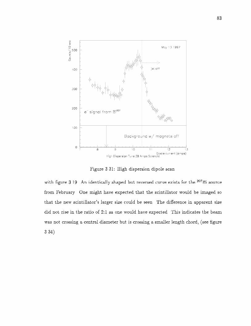
83
Figure 3.31: High dispersion dipole scan.
with �gure 3.19. An identically shaped but reversed curve exists for the 207Bi source
from February. One might have expected that the scintillator would be imaged so
that the new scintillator's larger size could be seen. The di�erence in apparent size
did not rise in the ratio of 2:1 as one would have expected. This indicates the beam
was not crossing a central diameter but is crossing a smaller length chord, (see �gure
3.34).

84
Figure 3.32: Low dispersion dipole scan.
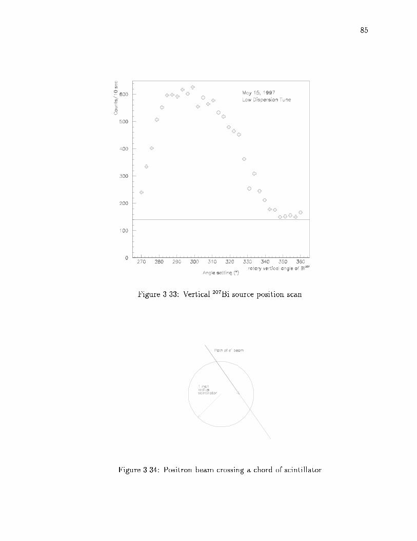
85
Figure 3.33: Vertical 207Bi source position scan.
Figure 3.34: Positron beam crossing a chord of scintillator.

Chapter 4
The E862 Antiproton Spectrometer
4.1 Time of Flight
Two fast plastic scintillator-fast phototube counters separated by 85 feet mea-
sured the time of ight of the antiproton. The time of ight clearly distinguished
accidentals. The resolution was not enough to distinguish antiprotons from charged
pions and kaons at the same beam momentum except at the lowest momenta. where
the �n could annihilate into a hadronic mode including pions. The pions would be
signi�cantly below beam momentum, closer to the �p velocity. The resolution for
on-momentum kaon rejection must be better than about 500 ps (FWHM) to get 3�
rejection except for momenta p> 8 GeV/c, as seen in table 4.1. This table shows the
di�erences in time of ight (nsec) between antiprotons and eitherK� or �� traversing
time of ight counters separated by either 85 or 95 feet. The table considers that the
kaons or pions are traveling at the same momentum. In other words no assumption
has been made about the process from which they originate.
Fast Pilot-U plastic scintillator paddles, the upstream one (200� 200� 1=800), the
downstream one (400�400�1=200) were separated by 85 feet. Coupled to two Amperex
XP-2262 phototubes each, they provided timing resolution of:
�t =q(�scint = 350ps)2 + (�pmt = 350ps)2 = 500ps (4.1)
86

87
Table 4.1: Required resolution to distinguish K� and �� from �p for equal momenta.K� ��
p(GeV/c) 85' 95' p(GeV/c) 85' 95'3.7 2.707 3.026 3.7 1.995 2.2305.6 1.179 1.318 5.6 0.868 0.9705.9 1.075 1.202 5.9 0.803 0.8986.2 0.946 1.057 6.2 0.700 0.7828.9 0.466 0.521 8.9 0.350 0.391
The counters were tested with cosmic rays at Penn State to characterize the
timing resolution. Figure 4.2 shows the setup used for the test. A pulse height
correction was made to remove time walk from discrimination at a �xed threshold,
(see �gure 4.3). Two cables lengths of RG-58 were attached (30 feet, 80 feet) and
FWHM of 500 ps was measured for the latter, (see �gure 4.5), after pulse height
correction. The cable lengths at Fermilab were >300 feet of RG-8, so the resolution
was signi�cantly worsened (1.6 ns FWHM) although not as much as would have been
the case with RG-58. The �nal counters had these PMTs with voltage dividers,
(see �gure 4.1), modi�ed for fast timing. The voltage applied to the phototubes
was determined by measuring the e�ciency (ratio of rate of the opposite PMT to
coincidence rate of two) as a function of applied voltage, (see �gure 4.6). There are
two analog signals from each PMT base. The signal taken from the last dynode is sent
upstairs as the ADC signal and inverted before being integrated. The anode signal
has a larger pulse height than the dynodes and thus less error on the arrival time. The
best precision on the timing pulse is obtained by discriminating after 10 ns of cable
and sending the digital pulse upstairs. These signals arrive over long cables but the
dispersion of the signals is known since the cable lengths are known. Unfortunately,
the discriminator delay is not known precisely. In addition, in January, 1997, the TF1
signals were ampli�ed 10X before being discriminated, adding extra indeterminacy

Figure 4.2: Cosmic ray test time of ight counters

89
Figure 4.3: Time of ight di�erence showing the e�ect of time walk from pulse heightdi�erences.
Figure 4.4: Time resolution for short, (30 ft) cables

90
Figure 4.5: Time resolution for longer, (80 ft) cables
Figure 4.6: High voltage plateaus for the time of ight counters.

91
Figure 4.7: Nonlinearity of one of the fast-TDC channels. The average resolution ofthis channel is 21 psec per least count.
to the upstream timing distributions. This was done in order to increase the trigger
rate by using all single electron noise (5 mV) events in TF11 or TF12 in coincidence
for part of the trigger.
The arrival times of the phototube signals from the plastic counters have un-
certainties associated with the detector resolution as well as from the error on the
conversion constants. A precision pulser was used to calibrate the TDC, and a sent
time vs. measured time curve was �t to a line to determine TDC conversion con-
stants, (see �gure 4.7), for a typical channel's response. The signals from di�erent
times di�er partly because of systematic errors arising from channel to channel di�er-
ences in the TDCs (�1 ps/LC) and each channel's nonlinearity (max: �5 ps/LC, avg:�1.2 ps/LC) which means di�erent conversion constants should be used for di�erent
arrival times within the same channel. We assign one conversion constant of 21.2 �1.5 ps/LC to all the TDC channels and arrival times.

92
4.2 Antiproton momentum measurement
4.2.1 Wire Chamber Description
The momentummeasurement of the antiproton after the �rst TOF counter uses
two dipole bend magnets and three wire chambers. The dipoles have di�erent lengths
but roughly the sameRBdL, corresponding to a bend angle of about 5o, as shown in
table 4.2.1. They are the only two spares for antiproton source ring magnets of their
type available. Two dipoles instead of one increases the bend angle. TheRBdL was
uniform across the transverse dimension to less than 5� 10�4 over �2.5 inches , (see�gure 4.8), and as a function of applied bend bus current was linear to 10�5, (see �gure
4.9). As discussed below, the main source of error in the momentum measurement
was multiple scattering, not �eld nonlinearity.
Table 4.2: Momentum analysis magnet parameters. As described in section 4.3, thecurrent settings had to be altered to center the beam.
Magnet Type Bend Angle Arc Length Radius of BMax
(mrad) (inch) Curvature (inch) (kG)Ideal magnet usage
SDE-007 106.281 98.425 926.083 12.613SDD-070 95.077 65.370 687.549 16.988
E862 magnet usageSDE-007 142SDD-070 93
Before, between, and behind the two dipoles are three multiwire proportional
chambers which have rectangular-shaped active areas of 600 � 400. They were used
with a previous Fermilab experiment, E690 [88], as beam pro�le chambers and were
characterized for e�ciency, but at a higher pressure (15-30 psig) than our use at STP.
They have 1 mm wire spacings, with wires arranged at angles of �7:1� and �21:6�

93
Figure 4.8: Characteristic nonlinearity of magnetic �eld across transverse dimensionof an antiproton bend magnet [67].
Figure 4.9: Nonlinearity of magnetic �eld as a function of applied current for anantiproton bend magnet.

94
with respect to vertical. The pulse seen at the preamp is about 10 nsec wide and has
a jitter of about 30 nsec due to the di�erences of arrival times of electrons to a wire.
The wire chambers had been assembled by E690 members by interleaving 0.001"
cathode foils in between signal wire planes and one foil each on either end of the
sandwich along with one ground plane on either end, (see �gure 4.11). G10 spacers
were used between cathodes and signal planes. The planes were mounted on alu-
minum frames, one on each end. The other face of the frames were capped with
Kapton/Kevlar windows designed to withstand high pressures.
The channels were read out with preampli�ers, (see �gure 4.10), in groups of
eight into discriminators located in crates in the tunnel near each chamber. The
discriminators were set at 150 mV. The discriminator pulses were read out over ANSLI
32 channel at delay cable which were between 150 and 260 feet long. The chambers
are spaced 40 feet from each other. The signals from the delay cable arrive at signal
conversion cards seated in standalone crates in the counting house. These converted
the signals to new signals suitable for the LeCroy 4291 TDCs. The TDCs recorded
one hit per trigger and were used in common stop mode. They were set to a resolution
of 1 nsec per least count for a total range of 512 nsec.
Since only one CAMAC crate of TDCs was available for use with the chambers,
we could instrument only 704 channels. This put a constraint on which planes and
sets of wires to use. Below is a table outlining the scheme best suited to measuring
the momentum.

95
Figure 4.10: Preampli�er schematic for each PWC channel [88]

96
Table 4.3: Wire chamber wires read out before run 10.Chamber Planes No. Wire/ No. Wires/Plane
plane rel to beam (No. �beam)1 1-4 32 �16 (��beam)2 1-3 64 �32 (��beam)3 1,3,4 128 �64 (�4.8�beam)
Table 4.4: Wire chamber wires read out after run 9.Chamber Planes No. Wire/ No. Wires/Plane
plane rel to beam (No. �beam)1 1,4 64 �32 (�2�beam)1 2 32 �16 (��beam)2 2,3 96 �32 (��beam)3 1,4 128 �64 (�4:8�beam)
3 96 �48 (�3:6�beam)

97
Figure 4.11: Breakdown showing the various planes of the wire chambers [88]

98
Before commissioning the wire chambers, small spots of residue from beam-
induced radiation damage were cleaned from the planes. New cathode foils were
glued on the frames and the wires were cleaned with solvent around the area where
residue was built up. Finally, a gain measurement was made to ensure equal gains
for all wires in a plane.
4.2.2 Momentum Resolution
The goal of the momentum measurement was to be able to resolve the on-
momentum antiprotons from antihydrogen from other tracks to a few times the beam
momentum spread of �pp= 2 $ 5 � 10�4. Material along the path gives the �p an
angular spread from multiple Coulomb scattering. Because the track angle changes in
the wire chambers due to multiple scattering, the momentum resolution is degraded.
The required momentum resolution sets a limit on the thickness of the TOF upstream
scintillator paddle, since the paddle was downstream of the �rst wire chamber and the
thickness of the chamber foils and target foils are �xed. It is a small e�ect, though,
and the primary reason for a thin counter is to have a small spot size on the wire
chambers downstream. Its thickness was 0.25" until run 21 when it was replaced with
a 0.125" thick paddle. There is also a 0.002" titanium exit window at the end of the
high vacuum region. Table 4.2.2 lists the contributions from multiple scattering from
the various materials. The end result is a best momentum resolution of 10�3 for a
3.672 MeV/c antiproton:

99
Table 4.5: Multiple scattering contributions at 3.7 GeV/c and 6 GeV/c.z(m) Location X0 �y ��y �y ��y
(mm) (mrad) (mm) (mrad)3.7 GeV/c 6 GeV/c
0 Jet (A50) 1.40 0.240 1.40 0.24015 A5B3 exit 3.86 0.240 3.86 0.24018 4.54 0.240 4.54 0.24018 400 �g/cm2 9:37 � 10�6 4.54 0.240 4.54 0.24019 4.77 0.240 4.77 0.24019 Ti window, 0.002" 0.000937
0.35" air 0.000329PWC (4 planes) 0.001531/4" scintillator 0.007484.2 mil Mylar 0.000376
TOTAL 0.01084 4.77 0.402 4.77 0.31037 5.75 0.402 5.38 0.31037 PWC 0.00153 5.75 0.417 5.38 0.31755 6.65 0.417 5.94 0.31755 PWC 0.00153 6.65 0.432 5.94 0.324
4.3 Antiproton Beamline Alignment
Before the antihydrogen running began, two calibration periods, consisting of
12 hours of dedicated antiproton beam down the E862 beamline, were used to align
the wire chambers. The chambers had been aligned on the beamline optically to a
precision of 1 mm, but the calibration periods provided a veri�cation using real beam.
One 2�sec shot of protons was projected on the antiproton target. That shot was
immediately transferred to the debuncher and then to the accumulator, where the
dipole A5B3 was shunted o� so that antiprotons would travel straight into the E862
apparatus. The target wheel was moved to a blank for fear of radiation damage to the
foils. The small dipole was left o� since the de ection at the calibration momentum
of 8.85 GeV/c would be di�erent than at the run momenta.
The large antiproton bend dipoles downstream were set for 8.85 GeV/c. The
wire chambers' high voltage was set at -1350 V. Because the TDCs are used nominally

100
with a 512 nsec gate, less than a quarter of the shot's antiprotons were able to be
recorded.
The �rst calibration period proved the readout of the PWC TDCs in the DAQ
worked properly but the distributions in transverse dimension and in time were at
in PWC #1 and PWC #2 and no sign of a beam spot was seen. In addition, PWC
#3 had a much lower rate. After the period was over, it was discovered that, a
vacuum isolation valve had been closed upstream. The beam was hitting the valve
and spraying secondaries down the E862 beamline. Secondly, one of the antiproton
dipoles in the E862 beamline was steering the beam o� by 1.3o because it was designed
for somewhat less current. To compensate, the beampipe downstream of the bend
magnets was moved to the outside by 1.3o (36.9 mrad).
The second calibration period was more successful. The same procedure of data-
taking was used. The resulting distributions across wires in a plane showed a beam
spot within the apertures of each chamber. The distribution of all hit times shows
3 peaks, one for each chamber, since the delay cables were such that each chamber's
hit times were separated from the others' by about 100 ns for a beam momentum
particle. The delay for the common stop signal on the PWC TDCs was set so that
the last quarter of the bunch was seen. Even so, the number of hits was large enough
that forming space points and tracks was di�cult. For subsequent tests, the beam
was scraped down in intensity (and in size). Events were recorded at about 3 Hz,
although each event had a couple of hundred tracks in the 500 ns window. About 30
events were accumulated in each run.
Once this had been established, various local de ections within the ring (or orbit
distortions) upstream of A50 were introduced to characterize where the beam spot
was located within the chambers and when the beam hit the edges of the chambers or
upstream apertures. Orbit distortions in angle and position for both the horizontal

101
Table 4.6: Left and right edges of the beam (inch)Perturbation X-left X-right Y-left Y-right j�Xj j�Y j
Standard Stacking -.223 -.498 -.126 .104 .275 .230Settings
Horizontal Angle -.236 -.291 .199 .072 .055 .127Horizontal Angle -.159 -.554 -.153 .001 .395 .154Horizontal Angle -.237 -.503 .094 -.167 .266 .261Horizontal Position -.229 -.432 .111 -.001 .203 .112Horizontal Position -.239 -.315 .089 .078 .076 .011Vertical Angle -.231 -.356 .136 -.336 .125 .472Vertical Angle -.220 -.464 .007 .063 .244 .056Vertical Position -.175 -.518 -.166 .095 .343 .261Vertical Position -.203 -.430 .058 -.205 .227 .263Standard Settings, -.194 -.454 -.078 -.101 .260 .179e+ dipole ONE835 angle -.171 -.375 -.180 .099 .204 .279
E835 angle removed -.205 -.507 .062 -.061 .302 .123septum 1 voltageseptum 2 voltage -.202 -.419 -.021 .134 .217 .155kicker voltage -.164 -.426 .266 .330 .262 .064
and vertical dimensions were tried. Changes in septum voltages and kicker currents
were also tried. Shown in �gure 4.12, are characteristic wire number pro�les (across
one plane) and a time pro�le, one peak for each chamber. Shown in table 4.3, are the
edges of the beam ascertained from the wire numbers of each plane which de�ned a
FWHM of the distribution across wire number in each plane. Each orbit distortion
or other perturbation is listed with the corresponding e�ect on the beam edges.
Finally, the last few tests were used to change the gains of the PWCs. Five
runs were taken at di�ering chamber voltages to get a rough look at the chamber
e�ciencies as a function of voltage. A voltage of -1350 V for all three chambers was
initially chosen as the operating point, although runs 10-13 used -1375 V and starting
with run 14, -1400 V was used throughout.

102
Figure 4.12: Typical transverse transverse pro�les by wire number for each PWC andtime distribution of hits showing 3 peaks arising from di�erent cable delays for the 3chambers.

Chapter 5
Trigger and Data Acquisition
5.1 Experiment Trigger
The basic antihydrogen requirement is to see a hit in the positron detector's
counter AND to see a hit in both of the time-of- ight counters. This three-fold
requirement was relaxed to less restrictive triggers consisting of the two-fold coin-
cidences of scintillator paddles. This allowed a more thorough characterization and
rejection of background in o�ine analysis. The coincidence of the two phototubes' sig-
nals from each time of ight counter, named TF1(upstream) and TF2(downstream),
reduced random noise since the raw rate of each phototube was on the order of 1
kHz. The TF2 coincidence (TF21 AND TF22) was made after the signals left the
PMT bases, travelled over 10 ns of cable and were discriminated. The individual,
discriminated signals went to TDCs, but the coincidence was sent over Heliax cable
(v = 0.88 c), high speed cable (same signal dispersion as RG-8), upstairs to arrive
closer in time with the upstream signals and eliminate delay cable. The signal from
TF1 was used in all triggers except H4 and was delayed to come second in time so it
would act as a time strobe. The signals in the coincidence triggers were set to overlap
by 75 nsec. Three antihydrogen triggers were built upon this:
� H1: TF1N e+
103

104
� H2: TF1NTF2 { This was the most restrictive needing all 4 TF PMTS.
No hit in the e+ arm is required so background tracks could be seen with this
trigger.
� H3: TF1 (prescaled) (usually by a factor of 100). The prescale factor was
determined so that the live time would be maximized for real antihydrogen
events.
� H4: TF2N e+ { Added after run 20 to see whether any antihydrogen events
were missing TF1 completely. Since it was not strobed to TF1, its absolute
timing was only close to the other triggers to within about 1 nsec.
Then the hits from all pmts except those attached to the NaI were read out as
a random PMT trigger (A1) in order to assess pedestals, etc.
� A1: E1L TF1LTF2
LT3
LT4
LV 1:::
Finally, to test the positron arm, an e+ counter only trigger (A2) was used to ac-
cumulate statistics when using the 68Ge source, especially since this could be done
without switching the power supply lugs.
� A2: e+ only
The rates from these triggers (averaged over runs) are shown in table 5.1:
The rates of the counters themselves scale with luminosity. The luminosity in the
following, (see �gure 5.2), is calculated from the beam current and jet density at the
time. The NaI is a coincidence between the NaI halves where both are discrimiated
at the 250 keV level. TF1 and TF2 are coincidences between the two phototubes
attached to each time of ight counter.

105
Figure 5.1: E862 trigger diagram.
Table 5.1: Overall E862 trigger rates for normal running conditions (beam).Trigger Rate (Hz)H1 6� 10�3 < R < 2� 10�2
H2 5� 10�4 < R < 3� 10�3
H3 1� 10�2 < R < 7� 10�2
H4 10�5 < R < 10�4
A2 4 < R < 20

106
Figure 5.2: Average rates from the counters as a function of instantaneous luminosity.
The trigger was built completely from commercial NIM standard modules.
CAMAC scalers were used to read out, as well as Fermilab-built visual scalers used
for rates.
5.2 Data acquisition
The channels consist of counters reading out to ADCs and TDCs and chamber
TDC hits. The expected rate of events for random coincidences contributing to the
TF1NTF2 trigger rate is 10�5 Hz. Using the other triggers allowed distributions of
measurements for background channels to be acquired. Data was taken at a rate of
a few Hz. An Apple Macintosh computer read out events through a Jorway CAMAC
interface. At this low rate, there was an average 97.0 % live time. The live time is
the ratio of total triggers to triggers recorded by the data acquisition. Most of the

107
dead time came from bursts of beam (few hundred/sec) during periods of signi�cant
beam loss when the data acquisition could only record a few events per second.
Every ten events, scaler channels recording rates of individual counters as well
as trigger rates were written along with high voltages into the datastream. Every 15
minutes, a unix workstation polled the Macintosh for new data �les and transferred
the �les to the workstation for writing to tape and analysis.
A preliminary analysis was performed on the data consisting of track forming
and cutting on expected energy and time windows. Events passing loose cuts were
dumped to �le and made available via the experiment web site. Antihydrogen can-
didates, as selected by triple coincidence, triggered a pager, as did alarms on high
voltage and data acquisition errors. In all, 129178 events resulting from jet-beam
interactions have been acquired and written to disk.
5.3 Target and Magnet Control
The control subsystems, run through the accelerator's ACNET interface and
network, made easy access for changing the position of the stripper wheel and con-
trolling the current through the magnets, (see section 2.1.3). The ACNET interface
page could be brought up on a workstation and issued commands to read or change
parameters.
The dipole (60A at 10V max) and solenoid (160A at 30V max) power supplies
could be operated in both voltage and current regulated modes. The power supplies
were controlled from (two) 0-10V analog levels from a 16 bit DAC (digital-analog
converter) which sat in a CAMAC crate near the supplies. While antihydrogen data
was being taken, the magnets needed to track the beam energy and, thus, the rest

108
24 - 5 V
T rigger N IM
C am ac
C am ac
A cc D iv V A X
Solen oid P.S.
D ip ole P.S.
U N IX w orkstation
M ac 7100
8200T ap e
H all Probe In terface
M otor
Sh aft En cod er
PC
PLC
V oltage C on verters
5 - 24 V
M otorD rive
Wheel
T D C s
RS232
SCSI
Ethernet
SCSI
DigI/O
R am p G en erators
Overall E862 Control------------------
ACNET (ethernet)
PLI
20 Hz
Once per15 min
Once per5 min
Once perstack
Figure 5.3: Data collection path and control of the magnets and target wheel.

109
of the ring's magnet currents which were available from a table setup on ACNET.
When a radioactive source was put in place, the current could be reset to that needed
to bend the positrons or electrons from the sources. Every time the electron source
was used, the polarity of the leads had to be reversed on both supplies by hand. As
described in section 3.5.3, the dipole had signi�cant hysteresis so it had to be ramped
back and forth a few times before settling down to a steady state I vs. B pro�le. The
currents were read out by a scanning, multiplexed ADC.
The target wheel was attached to one end of the shaft of a stepper motor. On
the back end of the motor, a shaft encoder recorded rotation angle changes at the
same resolution of 400 counts per revolution. This a�ects the resolution of the foil
vertical position. A feedback loop was implemented by using a micro programmable
logic controller to compare the number of steps seen to that given to the motor.
When a new position was requested, the wheel would be advanced to a zero point at
which the encoder sent out a pulse and then would be advanced the needed number
of steps. It was feared that the motor would mistep and this would eventually lead to
antihydrogens missing the active area. As well, the sources are much more localized
than the at stripper foils and thus bene�t from precise alignment of the wheel. The
�PLC was, in turn, controlled by a digital input/output card. When accessing this
ACNET 'device', one could download a new position or read back the current counter
level and status. The data written to, and read out through the ACNET system were
logged to a �le on the ACNET system's VAX. Every 5 minutes a copy was transferred
to the E862 workstation via an E835 workstation for monitoring and adding to lookup
tables.

110
ProgrammableLogicController
Motor Drive5 -> 24 V
Converter
24 -> 5 Converter
+24 V DC +5 V DC
1- Pulse2- Dir
3- AWO4- OptoIsol V
VacuumFeedthruMotor
Shaft Encoder
PLCOutIn
ToPC
PPI
From Acnet11 (5)bits
ToAcnet8 bits
ABZ
PulseTrain
Fuses
E862WheelControl
Zero Point
Figure 5.4: Target wheel control subsystem.

Chapter 6
Data Analysis
6.1 Introduction
The data �les were reconstructed by the o�ine code and scanned for interesting
events. An event was considered interesting if it contained a three-way coincidence in
time of the TF1, TF2, and e+ counter signals or alternatively an event with either a
hit in PWC #2 or, lastly, e+ counter and NaI signals consistent with a positron. The
original data �les were also subjected to a slower version of the o�ine code which
added information into the event structure about run numbers and beam parameters
such as beam momentum, emittances and beam centroid position. The data was
analyzed somewhat di�erently depending on whether the beam momentumwas above
or below the transition momentum of the accumulator (5196 MeV/c, section 2.1.2).
The data contains events taken with the foil target in place and those without the
foil target. The event variables used in the event selection are the number of tracks,
fractional momentum, vertical residual in PWC #2, extrapolated track positions at
the foil location or alternatively, at the location of the jet, pulse heights (ADC values)
and arrival times (TDC values) of the e+ scintillator, both sodium iodide halves, and
all four time of ight counter phototubes, and the veto counter arrival times.
The signature for an antihydrogen produced in the jet target is di�erent for
foil-in and foil-out data. With the foil in place, the antihydrogen is stripped of the
111

112
e+ within the foil. Ideally, the e+ traverses the magnetic spectrometer and hits the
middle of the plastic scintillator. It slows down, giving up all its kinetic energy to the
scintillator. It then annihilates yielding two back-to-back gamma rays. The gamma
rays should have an energy equal to the electron mass but may scatter within the
NaI detector yielding somewhat less. The antiproton will leave a beam momentum
track with no indication of a scatter. The track should point back to the jet since
it was formed there. When the foil is removed, the antihydrogen will not strip until
the vacuum window just before the �rst PWC is encountered. The e+ will muliple
scatter through almost all of the window with a mean angle which, in most cases, can
be seen as a hit in PWC #1. The antiproton will reconstruct as a beam momentum
track.
6.2 Antiproton beam data
The data obtained from ACNET (accelerator network) are shown in time plots.
The �rst two �gures, 6.1 and 6.2, are histories of the beam angle (in mrad) respectively
in the x and y dimensions over the course of the �xed target run. They come from
measurements of the beam position before and after the gas jet taken every 15 minutes
while the data acquisition was running. The x-axis represents an entry for each
measurement. The second set of two �gures, 6.3 and 6.4, show the emittances in
both dimensions plotted similarly. Finally, �gures 6.5 and 6.6 show the antiproton
beam centroid position extrapolated to the location of the foil target as a function of
(real) time. These beam parameters are used in chapter 7 to calculate geometrical
acceptances.

113
Figure 6.1: Horizontal angle during the run. The x axis represents one entry for eachmeasurement taken during running. The range is the entire �xed target run.
Figure 6.2: Vertical angle during the run. The x axis represents one entry for eachmeasurement taken during running. The range is the entire �xed target run.

114
Figure 6.3: Horizontal emittance during the run. The x axis represents one entry foreach measurement taken during running. The range is the entire �xed target run.
Figure 6.4: Vertical emittance during the run. The x axis represents one entry foreach measurement taken during running. The range is the entire �xed target run.

115
Figure 6.5: Beam centroid positions at foil extrapolated from beam position monitors8 meters upstream and downstream of jet (1996 data).

116
Figure 6.6: Beam centroid positions at foil extrapolated from beam position monitors8 meters upstream and downstream of jet (1997 data).

117
6.3 Track Reconstruction
The TDC information could have been used to operate the wire chambers,
as done with drift chambers, by weighting positions by hit times to get a resolution
�x < 100�m. In practice, demanding a window of �40 nsec around the mean time for
a particular chamber proved to be adequate. This eliminated noisy wires which had
random hit times. The distribution of reconstructed track positions in the chambers
for antihydrogen candidates showed a tight cluster of positions. Even so, the hits in
each event were separated by at least a few wire spacings, so using the times to tell
the di�erence was not needed. The di�erences between the mean times of the three
wire chambers were determined, by using delay cables, to be about 100 nsec. The
resolution for a position measurement was determined by the wire spacing (1 mm).
If two hits were on adjacent wires within 40 nsec of each other, they were considered
one particle (one hit) and the hit position was considered halfway between the wires.
The width of the arrival time distribution of electrons over di�erent wires is about 20
nsec wide. At least one hit in each of two di�erent planes of a chamber is needed to
record a space point. For events with 3 or 4 planes with hits, all hits were used. A
space point was calculated from two of them and the third had to be close in both
transverse dimensions (to within 1.5 wires) in order to qualify it as a true point. With
four planes hit, two points were made from two pairings and compared until one pair
of pairs were close in space. After run 20, there were no chambers with 4 planes and
a signi�cant fraction of events had only 2 planes of a chamber on. Thus many events
had a space point which was not well constrained. Occasionally, groups of adjacent
wires were on due to either a high energy particle knocking loose a delta ray or simply
from crosstalk in the discriminators.
All possible tracks were ascertained from the space points. For example, if only
one chamber had two space points and the other two chambers had only one each,

118
Figure 6.7: �2 distribution from �ts to space points in PWC #1 for candidates (solid)and all track events (scaled, dash-dotted).
two tracks were usually formed. The quality of the �ts to the space points making
up the track was characterized by a �2 variable, (see �gure 6.7).
A maximum of 15 tracks were found per event by the o�ine code. In practice,
less than 4 tracks were found per event except when the circulating beam started
to hit apertures and created a spray near PWC #1, (see �gure 6.8). The di�erence
between the measured x position in PWC #2 and that expected from the measured
x positions in PWC #1 and PWC #3, corresponding to their best space points, was
called the X-residual, (see �gure 6.9), and is related to the track momentum by:
Xres = Const � pcentral � (1p� 1
pcentral) (6.1)
The constant, Const = 49.340 inch was determined by a �t to the data.
The speci�c manner in which Xres is calculated is as follows: A straight line is
drawn between the hits in PWC #1 and PWC #3 in the coordinate system where
the central trajectory constitutes the longitudinal axis, (z). The deviation of the

119
Figure 6.8: Number of tracks per event
Figure 6.9: Diagram showing how the residual in the bend plane is measured.

120
Figure 6.10: Vertical (y) track residuals at PWC #2 for all events with one track.Arrows show cut based on wire chamber resolution.
Figure 6.11: Vertical (y) track residuals at PWC #2 for triple coincidence events.

121
hit's x position in PWC #2 from where the straight line predicts it should be is
denoted as Xres, the X-residual. The corresponding Y-residual in PWC #2, Xres,
is also calculated from the above method and should be equal to zero, in principle.
The cut on the Y-residual is established by the projection of the wire spacing in the
vertical and thus a jYresj < 0:15 inch was used. The triple coincidence events have
a Y-residual distribution contained within jYresj < 0:15 inch, (see �gure 6.11). The
tracks in general, however, have a gaussian Yres distribution with a much larger width
(� = 0:8 inch), as seen in �gure 6.10. The events falling outside of this cut are mostly
tracks that have undegone a scatter near the large antiproton bend magnets. For the
candidate events, a cut of jYresj < 0:15 has been adopted to keep only good tracks.
In fact, since we wanted to accept as many events with tracks as possible, we
accepted events in which one chamber had only one plane hit if the others had at
least two each. These tracks were classi�ed as a separate type since the PWC #2
residual in the non bend plane was assumed to be zero to make a straight line. There
was no way to cut such an event out if there was a scatter in that direction. The bend
plane Xres measurement in PWC #2 (used for the momentum) relied on horizontal
resolution which is better than the more vertical resolution by at least a factor of
two. This is because of the stereo angles of the chamber (�7o). The momentum was
better measured when >2 planes were hit in PWC #2.
The exact operating current of the antiproton bend magnets had to be de-
termined experimentally. These magnets derive their operating currents from the
accumulator bend bus (A:IB), as do all the dipoles of the ring, and used 50 mA
shunts to lower the current, by a maximum of 7%. The �rst antihydrogen candidate
was found with fractional momentum (0.990), signi�cantly di�erent from 1.000, and
having missed the TF2 counter. The fractional momentum is the ratio of recon-
structed track momentum to the beam momentum. After this run, the downstream

122
Figure 6.12: Saturation of magnets during deceleration ramps. The variable POFTTis the momentum of particles (MeV/c) which the magnets are supposed to bend. They axis is represents the ratio of applied current to magnetic �eld (normalized) andexhibits large hysteresis as the momentum is increased towards that of the injection.
bend magnet's shunt was adjusted to have a current 2% of the bend bus current. This
bent any subsequent tracks of the same momentum by 1/2" back onto the center of
the counter and the tracks registered a fractional momentum of 1.000. The ideal
shunt current was not known exactly because after deceleration the bend bus does
not always correspond exactly to the momentum. One reason is that the accumulator
dipole shunts are adjusted to get a certain geometry orbit and can be manipulated
without changing the overall energy of the beam. In addition, the accumulator mag-
nets were designed to operate well into the saturation regime at the injection energy
and a signi�cant amount of hysteresis a�ected the magnetic �elds at the lower beam
energies. The latter is technically a nonlinearity which could have been corrected for,
in principle. The second is much harder to correct for though.

123
Figure 6.13: PWC pro�les of all tracks with jYresj < 0:15. Noisy wires can be seen inPWC #2. Wires that de�ne the edges of each plane are shown.
The pro�les of the tracks on the wire chambers are shown in �gures 6.13, 6.14,
6.15. The wire con�gurations for runs 1-9 are di�erent from those for runs after 9.
Since only runs 6 - 9 correspond to data when the momentum scale was understood
well, these are not shown. The outermost wire of each plane instrumented is shown.
The �gures correspond to (runs 10-115) all events with good tracks, high momentum
(0:997 < ppbeam
< 1:002) events without evidence of a e+, and triple coincidence events,
respectively.

124
Figure 6.14: PWC pro�les of (non 3-way) high momentum tracks with jYresj < 0:15.Noisy wires can be seen in PWC #2. Wires that de�ne the edges of each plane areshown.
Figure 6.15: PWC Pro�les of tracks from three-way coincidence events with jYresj <0:15.

125
6.4 Antiproton Background Tracks
A quick calculation of the momentum acceptance of the spectrometer may be
obtained by recognizing that the magnets are very close to chamber 2 so the instru-
mented region in PWC #3 de�nes the momentum acceptance. Antiprotons below
96.15% of beam momentum (and above 101.9%) are not registered as tracks. There
are events in the data as far out as 95.35% and 102.75% (94.25% and 106.4% for
poorly �t tracks). The fractional momentum distribution shows a peak at 100% and
two larger peaks. Events with beam momentum above transition (p�p > 5:2GeV=c)
have a peak at about 97.5% of beam momentum while those below transition have a
peak at about 98.4% of beam momentum, (see �gures 6.17, and 6.18). Figure 6.22
shows the fractional momentum distribution for antihydrogen candidates which are
included in the previous two �gures. All the antihydrogen candidates have fractional
momentum >99.6%, except those which did not have a well-de�ned track and the
�rst candidate event (P=Pbeam = 0:990).
Understanding the background tracks is more important for the below transi-
tion data since signi�cantly more high momentum (P=Pbeam > 0:995) tracks were
recorded. A linear dependence exists, (see �gure 6.20), for the low momentum, back-
ground peak if fractional momentum is plotted versus beam momentum. Relaxing
the jYresj requirement allowed enough data to prove the acceptance of the antiproton
momentummeasurement apparatus was a function only of fractional momentum and
not of the beam momentum. This can be seen in �gure 6.20 where data �lls the
region between fractional momenta of 94.25% and 106.4%.
The secondary peaks in the fractional momentum distribution suggested the
antiprotons are scattering o� something. An antiproton could scatter by about -5o
(towards the outside of the ring) just before A5B3. It would then be bent 5o back to

126
Figure 6.16: Track/beam momentum for foil-in events in runs 1-115.
Figure 6.17: Track/beam momentum for foil-in events in runs 1-115 above transitionenergy.

127
Figure 6.18: Track/beam momentum for foil-in events in runs 1-115 below transitionenergy.
a centered trajectory pointing down the E862 beamline while traversing the magnet.
In doing so, some fractional (longitudinal) momentum is lost. The only explanation
which matches is elastic scattering o� single protons (hydrogen gas). It is reasonable
for a small amount of hydrogen gas to travel far from the jet. Figure 6.19 shows a
diagram of the elastic scattering. Figure 6.21 shows that the result for scattering o�
of helium atoms is far from the observed background peaks. It is clear that for larger
target atomic numbers, the momentum loss is smaller by Z2. Also shown is the e�ect
of a 10% error in theRBdL of the magnet. The A5B3 magnet has a bend angle of
0.0862 radian [67]. Extrapolating these tracks back to the area near A5B3 shows they
intersect the beampipe no more than 18" upstream of the beginning of A5B3 if the
-5o scatter is not included. This indicates the elastic scatter took place within 18" of
the upper edge of the magnet steel and not closer to the jet.
The amount of background gas in the vicinity of the A5B3 magnet can be
surmised from the number of tracks and the cross section for the scattering process.

128
Figure 6.19: Diagram of elastic scattering
The Rutherford scattering cross section is (Z = 1) for hydrogen[54]:
d�=d =Z2�2(F (q2))2
4p2sin4(�=2)(6.2)
Let's assume the proton form factor is equal to one. This can be integrated around
the 5o scatter needed to cancel the bend from the magnet. The angular range is
determined by the antiproton spectrometer's smallest aperture in angle drawn to
A5B3. The half aperture of PWC #3 is at most 2.5". Thus �� = 1:8 mrad. The cross
section is � = 0:0072=p2 or 76 nb for 6 GeV/c. The e�ective integrated luminosity for
1559 background tracks is now 20.5 nb�1. If this is compared to the instantaneous
luminosity and the total luminosity integrated at the jet, the instantaneous luminosity
for the background scatter process is found to be L = 4:7� 1027cm�2sec�1. Using an
average �gure for the number of antiprotons and revolution frequency, the background
gas density is:
�bkg = 1:8� 1010atoms=cm2 (6.3)
In order to get a density 2000 times smaller than the jet density, it is assumed that
the 5% of gas escaping from the region of the jet di�uses down the beampipe with an

129
Figure 6.20: Events with one track and jYresj < 0:1 inch. Background tracks withhigher beam momentum have a lower fractional momentum. Lines correspond toexpected ranges of large numbers of events.
approximately exponential pro�le. The above background gas density indicates the
1/e length is about 10 feet.
The curiously large number of P=Pbeam � 1:000 tracks below transition can most
likely be attributed to elastic scattering o� the aluminum beampipe. This is plausible
considering the larger emittance of the beam, below transition. The momentum loss
for scattering o� of aluminum is no more than �pp= 2 � 10�4 at 6 GeV/c which is
indistinguishable from a loss of zero.

130
Figure 6.21: Calculated elastic scattering o� hydrogen and helium superposed to showhow this accounts for the background, low fractional-momentum tracks. Many belowtransition tracks near beam momentum are thought to be scattering o� aluminumbeampipe. All events in this plot have only one track.

131
6.5 Secondary Backgrounds
Various background processes from the beam-jet interaction region have been
considered. Since the detector is so far downstream, the small solid angle suppresses
the overwhelming majority of possible background channels. The additional demand
that one particle be at the beam momentum (3-9 GeV/c) and the other be three
orders of magnitude lower in momentum (MeV/c) restricts the possible phase space.
This suppresses background channels which do not produce a near beam momentum
antiproton and a positron.
For example, the charge exchange reaction, �pp! �nn, will yield an antineutron
which can either beta decay or charge exchange back to �pp by hitting an obstruction.
The chance it does this near the foil is small. Reference [89] includes d�=dt as a
function of t for various reactions including �pp ! �nn at 7.76 GeV/c antiproton
momentum which is within our beam momentum range. The cross section at small
angles is about 2mb=(GeV=c)2. Let's assume the antineutron passes through the
A5B3 bend magnet and interacts within the �rst wire chamber where the beam spot
is only about 20 cm2, (see �gure 6.13). At a distance of 28 meters from the jet, the
solid angle is, at most, d = 2:6 � 10�6. The chance the �n interacts in the chamber
material is only 10�2. The number of antineutrons expected, found by integrating
d�=dt over �dt ' 4p2sin2 �2;=p2
2�d = 3:4 � 10�5, is 8:8 � 106 �n using 130 pb�1 of
integrated luminosity. The mean four momentum transfer in the reaction is about
9 � 10�3 (well outside the accepted solid angle) since the transverse momentum is
on the order of the pion mass (135 MeV/c). The chance the �n creates a �p when it
interacts is 4:9�10�3. This is the ratio of charge exchange total cross section to total
inelastic cross section (58 mb). Finally, the antineutron must have the correct angle to
make it to the last wire chamber. The chance it does this is 1:1�10�3 Altogether, the

132
number of double charge exchange events which could mock antihydrogen is expected
to be only 5� 10�1.
Other backgrounds were considered such as arising from long-lived neutrals
produced in the gas jet[90].
� �pp! KL +X; KL ! ��e+�, or KL ! �����e+�e:
The kaon has a 6:7� 10�4 chance to decay within 5cm of the foil target.
� �pp! ��o +X; ��o ! �p�+:
although lambdas are attenuated by 2 � 1023 over 10 m.
� �pp! �o +X; �o ! ! e+e�e+e�:
with an unrelated �p.
� �pp! �n! �pe+�:
The probability the �n decays within 5 cm of the foil target is 4�10�4, so similar
to the double charge exchange process, the number of �n is less than one.
The hypothesis that an antiproton interacts with the beampipe wall upstream
of the A5B3 bend magnet has been explored. If an antiproton traverses 20 cm of pipe
and only has multiple small angle Coulomb scatters, the antiproton only receives a
few mrad of bend. If on the other hand, it gets a large elastic scatter such that it
can bend by 5o and travel straight down the neutral beamline, the average loss of
longitudinal momentum is a few percent. See section 6.4 for more detail.

133
6.6 Foil Target-In Data
6.6.1 Description of Foil-In Data
Certain running conditions prompted consideration of only the runs where the
beam and detector were working properly. The parts of runs where stacking took
place were removed from the data set and stored as diagnostic data. Parts of runs 33,
68, 85, and 93 contained stacking periods. For runs 51, 76, and 77, the PWC interface
crate was o� so that the wire chambers' output was the result of unterminated cables
and lots of noise. Run 78 had the PWC discrimator crates o�. Run 75 had the e+
counter's base inadvertently removed. Runs 1-5 had the shunt of one of the antiproton
dipoles set incorrectly. The very �rst antihydrogen event was used to correct the shunt
current as described in section 6.4. In addition, runs 1-3 had incorrect delay cable
lengths for the e+ detector elements. Runs before run 14 had a PWC high voltage
setting lower than the nominal -1400 V used afterwards. The PWC hit e�ciency is a
strong function of applied voltage. Runs before run 21 had a di�erent PWC physical
con�guration. In runs after run 20, no antihydrogen candidates were seen in the region
of PWC #1 or PWC #3 which previously had not been instrumented. Finally, for
certain runs, the acceptance x e�ciency correction was quite small so these runs are
treated with special attention (beam steering acceptance, TF2 ine�ciency).
In the foil-in data, 78 candidates were observed. Of these, two had the signature
of the foil-out candidate events (high momentum track with spectator hit in PWC
#1) and are discussed in section 6.7. The remaining events had all or part of the
triple coincidence signature. Of the 76, eight were not triple coincidences at the trigger
level. Seven of these su�ered from the problem that one of the two phototubes needed
for the coincidence in TF2 (TF21NTF22), was found to be ine�cient towards the
later runs. The events were recorded since the TF1Ne+ trigger requirement was

134
met. Upon examination, all these events showed the other TF2 phototube to be on
as well as the existance of a beam momentum track. The TF2 trigger ine�ciency
is discussed in section 7.1. The eighth was the �rst antihydrogen candidate whose
antiproton track missed the TF2 counter. No events were seen which had a true
trigger e�ciency problem in the sense that some electronics mistiming prevented one
of the three triggers formed from the coincidence of two counters from �ring when
the other two did. I will call all of these triple coincidences since evidence was seen
of a signal either in the trigger or in the ADCs or TDCs from each of the counters
TF1, TF2, E+. The one exception to the rule is an event which did not have the E+
counter on but was considered because one of the NaI halves showed a pulse height
within the expected range. This event will be discussed as it may be a background.
Of the 76, 65 formed one track. Four did not form a track. Two of these were
in run 78 when the PWC discriminator crate was turned o�. Another was eliminated
because 3 of 4 of the hits in PWC #1 were too early. There is a 40 nsec time window
around the mean time for the chambers' signals. The last event was eliminated
because two chambers had only one plane hit. Neither could produce a space point
and a track could not be made. Of these 76 events, four have a beam momentum
below transition in all of 7.6 pb�1. The other 72 are above transition in a total of 77
pb�1.
6.6.2 Foil-In Momentum Distributions
Dealing with the above transition data �rst, the distribution of the ratio, recon-
structed track momentum divided by beam momentum, for those events having one
track is shown in �gure 6.22. It is a thin distribution of momenta around the beam
momentum. Figures 6.23, and 6.24 show these distributions, for above transition

135
Figure 6.22: Track momentum/beam momentum for triple coincidence candidates.The �rst event, ( P
Pbeam= 0.990), is not included.
and below transition respectively, superimposed upon all the data corresponding to
foil-in running for the same momentum range. The antihydrogen triple coincidence
candidates above transition nearly �ll the entire PPbeam
= 1.000 peak. The ratio of
candidates to high momentum track events without an e+ is about 2:1. Below tran-
sition, the situation is much worse, at least 30:1. This is thought to be antiprotons
scattering o� a metal aperture by 5o and being bent back by A5B3 by 5o in the oppo-
site direction. The mechanism is explained in section 6.4 for the case of a scatter o�
hydrogen. For aluminum, the fractional momentum changes by no more than 0.005
so there is no way of presently telling whether these tracks are not antihydrogen with
the present setup since the positron may be lost. This is not very plausible given the
knowledge of the e+ spectrometer. They are assumed to be scattered antiprotons.

136
Figure 6.23: Track momentum/beam momentum for triple coincidence events super-imposed on a histogram of the same variable for all events. Both are only abovetransition.
Figure 6.24: Track momentum/beam momentum for triple coincidence events super-imposed on a histogram of the same variable for all events. Both are only belowtransition.

137
6.6.3 Pro�les at foil
The set of tracks including antihydrogens can be extrapolated to the position of
the foil as well. Figures 6.25, 6.26, and 6.27 show the track positions at the foil, for all
tracks, for triple coincidence events (with tracks), and high momentumevents without
evidence of a e+, respectively. The �rst plot has the distribution of all tracks peaked
to one edge of the foil in the horizontal direction. The position on the foil one would
expect from using the positions of the antiproton beam centroid can be calculated as
well. The beam moves around quite a bit as can be seen in the plots of beam position
versus time, �gures 6.5, and 6.6. If the measured candidate event track positions are
subtracted from the calculated positions, the resulting distribution yields a measure
of the size of the antihydrogen beam at the foil location. Figure 6.28 shows the
measured foil positions of candidates after subtracting the centroid positions of the
beam obtained from ACNET information. The beam size expected from emittance
and ying wire measurements is �x � 0:300 at the foil.

138
Figure 6.25: Track position of all events with one track at the foil extrapolated fromPWC #1, PWC #2, PWC #3.
Figure 6.26: Track position of three way coincidence events at the foil extrapolatedfrom PWC #1, PWC #2, PWC #3.

139
Figure 6.27: Track position of high momentum events without an associated e+ hitat the foil extrapolated from PWC #1, PWC #2, PWC #3.
Figure 6.28: E�ective size of the antihydrogen beam. Position spread of candidateevents at the foil location corrected for beam position.

140
6.6.4 Emittance Measurements
The emittance of the beam can be ascertained by looking at the tracks recorded
by E862. Figures 6.29, 6.30, 6.31, and 6.32 show the transverse phase space plots
(x; �x); (y; �y) for triple coincidence events and all tracks. The emittance is the area
of the occupied phase space, �x = � ��x ���x . An ellipse has been drawn to give an ideaof how much phase space area the points �ll up and what emittance this corresponds
to. However, the ellipse shown is not a �t and does not correspond exactly to an
ellipse which encloses 95% of the particles. Furthermore, the ellipse is centered at the
origin. The events represented in the �rst plot, �gure 6.29, form an occupied area
which is clearly not centered at the origin. In addition, the position and angle o�sets
of the beam have not been removed.

141
Figure 6.29: X-Phase space plot of tracks for candidates.
Figure 6.30: Y-Phase space plot of tracks for candidates.

142
Figure 6.31: X-Phase space plot of tracks for all tracks.
Figure 6.32: Y-Phase space plot of tracks for all tracks.

143
6.6.5 Pro�les at jet
The track is extrapolated back to the gas jet by projecting where the PWC #2
space point would be if there were no bend and then drawing a straight line through
the space point in PWC #1, (see �gures 6.35, and 6.36). The track positions at the
location of the jet in �gure 6.36 form a rectangular pro�le, which may correspond
to the rectangular shapes of the dipole magnets' vacuum pipes. This could be due
to either the A5B3 dipole whose vertical aperture is only 1.45" (ID) or one of the
antiproton bend magnets P1, P2 which have apertures of 2.0" (ID). Figures 6.37, and
6.38 show the distributions for events separated into above and below transition sets.
Alongside the triple coincidence positions are positions for high momentum events
without evidence of a positron. Those below transition seem to �ll a large region
consistent with a rectangular beampipe pro�le. The e+ dipole magnet adds a small
but noticeable o�set of 0.4". The candidate track positions at the location of the jet
are o�set from the origin (see �gure 6.35).
One may ask if there is a di�erence in angular distributions of tracks from triple
coincidence events and tracks from high momentum events with no e+ by looking
at their angular distributions. If the latter are indeed mostly scatters o� a vacuum
pipe, then the angular distribution should at least �ll the angular acceptance of
the antiproton spectrometer. Figures 6.33, and 6.34 compare these distributions.
Although the triple coincidence events' angular distribution is thinner and clearly
more gaussian in shape, the high momentum (no e+) angular distributions are not
at. The X angles have been corrected by -0.38 inch due to the e+ dipole bend.

144
Figure 6.33: X angular distributions for triple coincidences and high momentumtracks without a e+. An o�set of 0.4 inch from the small dipole has been removed.

145
Figure 6.34: Y angular distributions for triple coincidences and high momentumtracks without a e+.

146
Figure 6.35: Extrapolated position of track at gas jet for triple coincidence events.The track positions are o�set horizontally from zero because of the e+ dipole (by0.4").
Figure 6.36: Extrapolated position of track at gas jet for all good tracks. The trackpositions are o�set horizontally from zero because of the e+ dipole (by 0.4").

147
Figure 6.37: Extrapolated position of track at gas jet for triple coincidence events,above transition. The track positions are o�set horizontally from zero because of thee+ dipole (by 0.4").
Figure 6.38: Extrapolated position of track at gas jet for triple coincidence events,below transition. The track positions are o�set horizontally from zero because of thee+ dipole (by 0.4").

148
6.6.6 Positron Energies and Annihilation Spectra
Of the 76 triple coincidence events, none had the veto counters on. This in-
dicates that the particle hitting the e+ counter came from the direction of the e+
spectrometer. The e+ counter energy deposits for all but one of the 76 clustered
around the energy value expected from the calibration data. None had energy de-
posits much larger than expected. A signal corresponding to a MIP is expected to
leave a much larger energy deposit in the counter.
There is a di�erence between data before and after January 1, 1997, since the
TF1 counter's threshold was lowered, (see section 6.6.7). This caused the triggers'
start signal as well as the ADC gates to be earlier and the ADC values larger.
Previously, the ADC signals were cut o� on the front end by a small amount and
had lower integrated values as a result. There was expected to be a change of the
gain when the 1" diameter scintillator (BC-418) was replaced with a 2" diameter
scintillator (BC-420) but none was observed (April 1997). In addition, the responses
for electrons and positrons were compared. No di�erence resulted.
The dependence of ADC values on dipole current was �t for the two cases and
used to convert to e+ energy (see �gure 3.30). The distribution of e+ pulse heights,
(in ADC counts out of a full scale of 1024), is shown in �gures 6.39, and 6.40, with
the 1996 and 1997 �ts to the calibration data, respectively. The pulse heights for
the triple coincidence events agree with the extrapolations to the calibration data.
Figures 6.41, and 6.42 show the deviation of the triple coincidence candidate events
from the extrapolation for 1996 and 1997 data sets, respectively. During April 1997,
the 1" counter was replaced by the 2" counter but no change in gain was observed
after repeated testing even though the scintillator material is di�erent as well. Thus
only two sets of gain constants are used.

149
Figure 6.39: Pulse height of e+ scintillator vs. e+ momentum for triple coincidencesduring 1996. A linear and a quadratic �t to the calibration data are shown.
Figure 6.40: ADC of e+ scintillator vs. e+ momentum for triple coincidences during1997. A linear and a quadratic �t to the calibration data are shown.

150
Figure 6.41: Deviation of e+ pulse heights from quadratic �t for 1996 triple coinci-dences.
Figure 6.42: Deviation of e+ pulse heights from quadratic �t for 1997 triple coinci-dences.

151
Figure 6.43 shows the e+ pulse height distributions for triple coincidence events
superimposed on top of the same distribution for all events, except the number of
events per bin has been scaled down by a factor of 1/1000. The ADC values of the
events from 1996 are scaled by a factor representing their di�erent gain constant. The
constant used here is the e+ peak of the pulse height distribution taken at the peak
of the �+ spectrum during calibration. Here the separation of the pulse heights from
the majority of the smooth background distribution is emphasized. If the triple coin-
cidence pulse height distribution were much more spread out, one might argue that
the hits were from other particles in the environment. They are all contained in one
small area. In addition, the dependence on beam momentum has not been removed.
Although the pulse height has been observed not to be exactly proportional to kinetic
energy deposited, there is still a well-behaved dependence on the e+ momentum. The
momentum dependence has not been removed in the previous �gure but it has been
removed in �gure 6.44. Figure 6.45 shows the distribution of e+ pulse heights for
events with one track only. Those events with one track that have a pulse height are
above pedestal, (about 60 counts), are almost all antihydrogens. Events with a lot
of spray from the jet region almost always have more than one track, so these are
excluded.

152
Figure 6.43: e+ pulse heights for triple coincidence events superimposed on the dis-tribution of pulse heights for all events. Events before run 20 have been correctedfor a di�erent gain constant. The histogram representing all events has been scaleddown by a factor of 1/1000.

153
Figure 6.44: e+ pulse heights for triple coincidence events superimposed on the dis-tribution of pulse heights for all events. Events before run 20 have been correctedfor a di�erent gain constant. The histogram representing all events has been scaleddown by a factor of 1/1000. Beam momentum dependence has been removed.

154
Figure 6.45: e+ pulse heights for all events with one track and three-way coincidenceswith one track.

155
The NaI energy deposits are trickier since the detector is much less e�cient than
the e+ counter. The distribution of NaI energy for candidates is the same as what is
seen in the calibration data though (see �gure 6.46) taken with the germanium �+
source. Figures 6.48, and 6.47 show the correlation of energies in the NaI halves for
triple coincidence candidate events and all events respectively. There are no huge
energy deposits in the candidate data which would indicate high energy photons
(at least a few MeV). The sodium iodide energy deposits are not used as a strict cut
since the e�ciency of seeing two 511 keV photons is only 30%, (see table 3.5). Clearly,
many events have both energies corresponding to 511 keV annihilation gamma rays.
This still represents only about 30% of the total. Approximately, another 30% have
energies in the bands where one energy is about 511 keV and another has lost some
energy due to a Compton scatter. Furthermore, some events exist along the band
where the sum of energies adds up to 2*511 keV. These indicate the scattered photon
was not lost but instead, entered the other half to contribute its energy there. Finally,
a very small number of events exist with larger energies in both halves. The events
where one of the energies is still in the 511 keV band are probably due to the other
energy value resulting from a photon which has a conversion very close to one of the
three phototubes. The increased solid angle may yield a larger pulse height than
average. The others are, most likely, annihilations in ight. The calibration data
shows this e�ect too and the proportion of events in the calibration data and the
candidates is approximately the same. Those events for which
E ;1 + E ;2 � 2 � 511keV (6.4)
is satis�ed were not cut. The reasons for an asymmetric energy deposit in the NaI
are discussed in section 3.6.3.
Very few background positrons were seen, probably because any created in or
near the jet would be bent by magnetic �elds far upstream. Neutral pion conversions

156
Figure 6.46: Correlation of e+ annihilation ray energies in sodium iodide for calibra-tion data
Figure 6.47: Correlation of annihilation X ray energies in NaI detector for all eventsin data.

157
Figure 6.48: Correlation of annihilation X ray energies in NaI detector for candidateevents in data.
with a Dalitz decay are frequent but they need to have the correct trajectory. For
example, for two pion modes, d��o�o=dcos�� is probably � 1�b near � =0 at 6 GeV/c.
The �o decays almost always to . One of the photons needs to travel with a
trajectory close enough to an antihydrogen that hits the foil. The probability that
the photon produces an e+e� pair near the foil determines the number of events the
experiment should have seen in 120 nb�1 to be about 2 � 10�2. Further reductions
come from the positron needing to have the correct trajectory and energy to traverse
the e+ spectrometer.

158
Figure 6.49: Annihilation X ray energy distributions from the NaI detector for allevents in foil-in data.

159
Figure 6.50: Annihilation X ray energy distributions from the NaI detector for triplecoincidence events in foil-in data.

160
6.6.7 Timing Analysis
The antiproton time of ight distributions are found by the di�erence in arrival
times between the TF1 and TF2 counters after corrections are applied. The correla-
tions of the time of arrival with the pulse height in the ADC and track positions are
taken into account by using a correction determined from accumulating and �tting
all good tracks which triggered both counters. The timing distributions of the TF1
and TF2 counters were correlated to the particle's position when passing through the
scintillator counter, (see �gure 6.51). Since each counter was close to the correspond-
ing wire chamber in the longitudinal direction, the wire chamber hit position was
used as the particle's position in the counter.
The corrections to the arrival times for the time of ight counters are calculated
by two methods. The �rst averages the signals from the two PMTs on each counter.
The advantage to this is that no �tting error results. It can be used to remove the
position dependence of a hit but not an arrival larger pulse height in both PMTs. If
both PMTs have the same gain, they will see equal pulse heights and arrival times
for a particle passing equidistant between them. A hit that is nearer to one of the
phototubes will generate more light near that phototube, less in the other and will
be averaged out. The problem is that two particles that leave substantially di�erent
dE=dx have di�erent arrival times because of slewing. If the two time of ight counters
had the same thickness (which they don't), this would cancel in principle.
The second method corrects the timing distributions of each counter for pulse
height and position dependence independently. As described in section 6.4, the back-
ground tracks are predominantly antiprotons very close to beam momentum. Their
pulse height spectrum and corresponding arrival times are expected to be distribu-
tions with small widths. Once the particle's position dependence has been removed,

161
the arrival times are not correlated with the pulse height spectra. It will su�ce then
to use the averaging method for calculating the arrival time and the time of ight.
For the following analysis, a sample of events was de�ned by demanding that
the number of tracks be equal to one (except for candidate events), the absolute Y
residual of the primary track be less than 0.15 inch (jYresj < 0:15) and that the relevant
TDC channels all have in-time hits. They are all the above transition momentum of
the antiproton source. In addition, for the time of ight distributions, the ratio of
reconstructed momentum to beam momentum must be within the range, (0:9975 <
ppbeam
< 1:0015). The fractional momentumand Y residual are discussed in more detail
in section 6.3. A linear correction was applied to TDCTF11 vs XSP1, the horizontal
space point in the �rst wire chamber. This also removed the correlation of TDCTF11
with ADCTF11 and ADCTF12, (see �gures 6.52, and 6.53). A correlation with
TDCTF12 had to be further removed. The TDCTF21 and TDCTF22 distributions
have a dependence on the YSP3 (the vertical space point in the last chamber), (see
�gure 6.54), since these PMTs are aligned on top and bottom of the 4" wide counter.
The dependence of one PMT's arrival times on YSP3 is the reverse of the other PMT's
arrival times.
TDCTF21 � + :25 � Y SP3 (6.5)
TDCTF22 � � :25 � Y SP3 (6.6)
Any further dependence of TDCTF21 on ADCTF21 or ADCTF22 is not evident as
seen in �gure 6.55. The TF12 signal was the timing start (or strobe) for the two
higher rate triggers. The di�erence TDCTF11 - TDCTF12 is used to establish the
timing resolution of the TF1 counter as shown in �gure 6.56 with a resulting � = 0:4
ns spread after the correction for position is made. The resolution for TF2 is shown
in �gure 6.57 with a resulting � = 1:3 ns spread. Data with di�erent beam momenta
(and thus di�erent �) have been used so this has been factored out and the time of

162
Figure 6.51: Correlation of TF11 arrival times with horizontal position.
Figure 6.52: Correlation of TF11 arrival times with ADC TF11 after removing posi-tion dependence.

163
Figure 6.53: Correlation of TF11 arrival times with ADC TF12 (trigger start PMT)after removing position dependence.
Figure 6.54: Correlation of TF21 arrival times with vertical position.

164
Figure 6.55: Correlation of TF21 arrival times with ADC TF21.
Figure 6.56: Timing resolution of TF1 with and without position dependence re-moved. The resolutions are �1 = 0:44 ns and �1 = 0:71 ns respectively.

165
Figure 6.57: Timing resolution of TF2 (�2 = 1:3 ns).
ight normalized to the time of ight for � = 1. Part of the spread in time of ight
comes about because even at some �xed central beam momentum, the antiproton
beam has a velocity spread related to its momentum spread, (�p=p � 2� 10�4).
The time of ight is calculated using the two methods as follows:
Average:
TOF = ((TDCTF11 + TDCTF12)=2 � (6.7)
(TDCTF21 + TDCTF22)=2) � 0:0212 ns=LC � � + 88:96 ns (6.8)
Corrected:
TOF = (TDCTF11� 70 �XSP1 � (6.9)
TDCTF21 + 0:25 � Y SP3) � 0:0212 ns=LC � � + 88:96 ns (6.10)

166
Figure 6.58: Time of ight distribution using method 1, normalized to � = 1. Allevents have good tracks with high momentum.
The distribution of the time of ight for the averaging method and the removal
of correlations method are shown in �gures 6.58, and 6.59. Approximate gaussian
shapes are noticeable, but not much larger than that expected from the measured,
individual counter resolutions � =q�21 + �22 = 1:9 ns. The top plot in each is the
normalized time of ight for candidate events, the bottom plot is that for all tracks
passing the selection criteria above. Clearly, the time of ight distributions show only
one peak, meaning only one type of particle can be distinguished. This is consistent
with the hypothesis that the dominant background in the antiproton spectrometer
is antiprotons being lost from the beam. Accidental coincidences in the counters are
distributed completely randomly in time. Most of these can be removed from the
event sample.
Because of the low rate environment, most of the events passing the TF1Ne+
trigger are expected to have hits in the two counters which are correlated in time (to
within a couple of ns). The time of ight di�erence between the two counters is about

167
Figure 6.59: Time of ight distribution using method 2, normalized to � = 1. Allevents have good tracks with high momentum.
6.5 ns. In �gure 6.60, one can see all the TF1Ne+ triggers showing most peak around
6.5 ns di�erence. A few are random hits perhaps of two unrelated antiprotons lost
from the beam. The antihydrogen triple-coincidence candidates clearly are clustered
around a 6.5 ns time di�erence.

168
Figure 6.60: Time di�erence between TF1 and e+ for all TF1Ne+ triggers and
candidate events. Only events from runs 21-115 were chosen.

169
6.7 Foil Target-Out data
6.7.1 Description of Foil-Out Data
In order to really test the hypothesis that the triple coincidence events recorded
were indeed antihydrogen, some data was taken with the foil target rotated out of
the way, leaving a hole, 1" in diameter. After run 50, this hole was increased to 1.75"
in diameter. The wheel is 1/32" of aluminum. No triple coincidences were expected
and none were observed. An antihydrogen that ies through the hole will also pass
through the e+ dipole with no e�ect. It will ionize in the 0.002" titanium vacuum
window 3.25 inches upstream of PWC #1. Because of the material, the positron
will multiple scatter in 0.14% of Xo by 7o at p�p = 6 GeV/c (or 13 mm = 13 wires
on average). Thus the positron and antiproton register separate hits in the wire
chambers. The e+ still is usually within the acceptance of PWC #1.
The �rst indication came in the �rst 5 pb�1 of target-out data. Four events
with beam momentum (p�p > 0:995) tracks were seen. Three of them had at least
one second hit in PWC #1 in one of the planes. Some had a hit in each of all three
planes of PWC #1 that did not corresponding to the antiproton track. None had
extra hits in the other two wire chambers. The data are therefore consistent with
the antihydrogen hypothesis. If one expects that the events are not antihydrogen and
the stripping foil has no e�ect, then the probability of getting no triple coincidences
when one expects roughly �ve (based on the triple coincidence rate with foil in place)
is 0.7%. Also, if an antihydrogen cross section of 0.8 pb is assumed, the probability
of seeing three candidates out of 5 pb�1 is 19.5%.

170
Figure 6.61: Transverse position of track at location of jet for foil-out antihydrogencandidates as well as beam momentum tracks without evidence of a e+.
In all, 25 foil-out candidates were observed. Twenty-one had a beammomentum
above transition in all of 33 pb�1. The below transition, foil-out data corresponded
to an integrated luminosity of 7 pb�1.
6.7.2 Jet Location
Figure 6.61 shows the distribution of transverse positions of the antiproton
tracks at the location of the jet for foil-out antihydrogen candidates as well as beam
momentum tracks without an extra hit in PWC #1. Figures 6.62, and 6.63 show the
same distributions split up into above and below transition data respectively.

171
Figure 6.62: Transverse position of track at location of jet for foil-out antihydrogencandidates as well as beam momentum tracks without evidence of a e+. Only abovetransition events are displayed.
Figure 6.63: Transverse position of track at location of jet for foil-out antihydrogencandidates as well as beam momentum tracks without evidence of a e+. Only belowtransition events are displayed.

172
Figure 6.64: Fractional momentum distribution for foil-out candidates superimposedupon that for all events during foil-out running.
6.7.3 Momentum Distributions
Figure 6.64 shows the distribution of the ratio, reconstructed track momen-
tum divided by beam momentum, for foil-out candidate events superimposed on the
distribution for all events from the foil-out data both sets corresponding to above
transition only. The candidate events are clustered around a fractional momentum
of ppbeam
= 1:000.
Figures 6.65, and 6.66 show the distribution of the ratio, reconstructed track
momentum divided by beam momentum for foil-out candidate events on top of the
distribution for all events from the foil-out data, for above transition and below
transition, respectively. Only four foil-out candidate events are shown in the below
transition data. Only two are truly near a fractional momentum of ppbeam
= 1:000.
The other two are most likely, from the tail of the elastic scattering peak as discussed
below.

173
Figure 6.65: Fractional momentum distribution for foil-out candidates superimposedupon that for all events during foil-out running, both for above transition running.
Figure 6.66: Fractional momentum distribution for foil-out candidates superimposedupon that for all events during foil-out running, both for below transition running.

174
The reconstruction and unambiguous determination of the events involved sep-
arating out the correct track from the multiple tracks formed. All hits were paired to
form possible space points in the wire chambers. If the spectator had hits in multiple
planes, it could form a valid space point. If not, it might still pair with one of the
antiproton hits to make an incorrect space point. Similarly, when the space points
in PWC #2 and PWC #3 are considered to make a track, they might be associated
with either the e+ space point or the space point formed from the incorrect pairing
of e+ and �p hits to give an incorrect track. These tracks are not extremely di�erent
from the true antiproton track in fractional momentum (� � 0.003) but have much
larger y residuals.
Below transition, only four foil-out candidates were observed. Only two are truly
antihydrogen. The other two are most likely background from the tail of the elastic
scattering distribution. Figure 6.66 shows the fractional momentum distribution for
these events against a histogram of all events in the below transition, foil-out running.
One notices the two antihydrogen events have fractional momentum close to 1.000.
The fractional momentumof the other two are di�erent from 1.000. There is a possible
systematic error from lack of knowledge of the proper shunt current for the antiproton
dipole at each momentum. On the other hand, the location of the elastic scattering
peak is almost a completely linear function of beammomentum. The elastic scattering
peak location can be used to correct the fractional momentum of candidates. Because
it is a small e�ect, it was not performed on all candidates. It was looked at especially
for these events, though, in hope that the two background events had the momentum
scale incorrect. However, after correction, the two events still remain about where
they were in fractional momentum. In support of the background hypothesis, it
should be noticed that both events had larger than usual Y residuals (jYresj > 0:2
inch).

175
As in the foil-in data, there are beam momentum events without any evidence
of a positron. Above transition, the ratio of these events to candidate events in the
foil-out running is approximately 1:2 (actually 12:21). Below transition, the ratio
is much larger (62:2) resulting from a larger beam hitting beampipe or steel. This
should be compared to the foil-in ratios: above transition (31:61) and (63:3) for above
and below transition respectively. The existence of a good track is assumed.
6.7.4 Background to Foil-out Candidates
There are three classes of events indicating a possible background for the anti-
hydrogen candidates.
Two candidates having the foil-out signature show up in the foil-in data. These
are interesting as a possible background to the foil-out antihydrogen candidate events.
Only one event was above transition. The �rst event clearly shows two particles
passing through the chamber separated by a few wires in each of 3 planes. The
second lists adjacent wires in the �rst plane but plane 2 and 3 have separated wires
on. Both of these suggest either an unstripped antihydrogen or a beam momentum
antiproton kicking out an electron.
Two of the foil-out, below transition events are close to the candidates in frac-
tional momentum and the number and placement of extra hits in PWC #1. The
fractional momentum and/or Y residual are di�erent enough to exclude them as can-
didates but not by much.
Three of the triple coincidence events have extra hits in PWC #1 (which are
not adjacent hits). Of these, one has no e+ counter signal but one of the NaI halves
registers a 511 keV gamma ray. This one has hits which are all adjacent. It can
therefore be excluded since there is no justi�cation that the hits are from a separate

176
particle. The second event has a strange timing scenario in which the hits associated
with the antiproton are early and an extra hit in the �rst plane is a bit late. This and
the third event are probably antihydrogen where the antiproton kicked o� an atomic
electron.
One possibility was that an antihydrogen found a hole in the carbon foil or that
it traveled through the foil without ionization. The stripping is >99%. If it is equal
to 99%, the probability of observing one unstripped event out of 73 events (observed
as candidates) is 0.35 and would be closer to one except for the uncertainty resulting
from the statistics of small numbers.
Another possibility is that an antiproton can knock an orbiting electron out of
a titanium atom in the vacuum window 3.2500 upstream of PWC #1. The electron
will multiple scatter and lose some energy but if it gets out of the titanium, it may
be seen as an extra hit in PWC #1 (if it is within the acceptance). This can happen,
of course, whether or not the antiproton results from an antihydrogen. The number
of electrons per antiproton resulting from an antiproton of momentum 6 GeV/c with
energy greater than E is given roughly given by the ratio ofW=E where (x= thickness
of window in �g=cm2) [91],
W (MeV ) =0:15
�2Z
Ax = 1:63 keV (6.11)
The e� must have enough energy to get out. A minimum ionizing electron would
have lost only 37 keV and the number of e� with E > 37 keV is equal to 0.044.
Since we require a beam momentum track, the number of beam momentum tracks,
above transition, which could have knocked out an e� is only about 100. The number
of expected background would thus be 4. This is an extreme upper bound though
since electrons with energies somewhat less than the rest mass lose substantially
more energy. Electrons with kinetic energies around a couple of hundred keV lose
start to lose a signi�cant fraction of that energy so I have assumed 200 keV to be

177
Table 6.1: Interesting events with extra hitsRun Event Frac. Mom.
Below transition, foil-out61 919 1.00062 675 0.99664 1430 1.005115 226 0.998Extra hit candidates in foil-out running70 1161 1.00072 2203 0.999Triple coincidences with extra hits
38 278 0.99940 1476 1.00081 2377 0.999
the threshold for getting out of the titanium. Lower energy electrons are scattered
more transversely and have less chance of being within the acceptance. For 100 beam
momentum tracks, only 0.6 events of this type are expected.

178
6.8 Event Selection Summary
Here are summarized, the cuts chosen to maximize the chance we were looking
at antihydrogen and not background. The antihydrogen signature for the foil-in
condition was background free. The zeroth order requirement of a triple coincidence in
the trigger was enough to isolate the antihydrogens during normal running conditions.
It is true that some data was inadvertently taken during high beam loss periods. The
rate of triple coincidences went up signi�cantly during these periods. The events were
clearly not antihydrogen though. This was evident by the multitude of hits and tracks
formed as well as by the random distribution of energy deposits in the positron and
gamma ray detectors. These running periods were removed from the data used to
determine candidates but served as a monitor of detector performance. The triple
coincidence trigger events during normal running all either had one, reasonably good,
near beam momentum track or did not have enough hits to form a track. Nearly
all had a hit in the e+ scintillator with energy deposit close to that expected for
antihydrogen.
The antihydrogen signature during foil-out running was more demanding. If the
positron hit in PWC #1 formed a space point with an unassociated hit in another
plane (due to the antiproton), more than one track resulted. If one track had the
momentum closest to beam momentum and the smallest Y residual, the track was
chosen as that of the antiproton. If not, the hits were examined by hand to determine
which space points were being formed correctly. The extra hit in PWC #1 had to be
signi�cantly separated from the antiproton hit. If they were less than 2 wires apart,
the o�ine code would think they were an associated hit due to a particle passing in
between two wires. As discussed in chapter 7, the ine�ciency from this condition
could be modelled.

179
Table 6.2: Event selection criteria for antihydrogen candidates.Triple Coincidences
0.996 < p=pbeam < 1.002jYresj < 0:15 inchNumber of tracks = 0 or 1100 < e+ ADC < 450 countsCoincidence of all three triggers, not
just all three counters.TF counter signal times consistent with beam particleEnergy deposit in either NaI half < 250 countsTransverse position at jet location consistent
with production in jetTransverse position at foil location
inside foil radius
Table 6.3: Event selection criteria for antihydrogen candidates.Foil-Out Candidates with Spectators
0.996 < p=pbeam < 1.002jYresj < 0:15 inchNumber of tracks > 0One clear, extra hit in at least one plane of PWC #1No energy deposits in NaINo energy deposit in e+ scintillatorTF1
NTF2 trigger on but no others
TF counter signal times consistent with beam particlePosition at jet location consistent with
production in jetTransverse position at foil location
inside foil radius

Chapter 7
Geometrical Acceptance and
E�ciencies
7.1 Simulation of foil-out candidates
The geometrical acceptance � reconstruction e�ciency for foil-out candidates
was simulated with an EGS4(NRCC version) [92] Monte Carlo program. During the
foil-out running, antihydrogen would ionize in the titanium vacuum window just be-
fore passing through the �rst wire chamber. The positron receives multiple Coulomb
scatters while in the high Z titanium but is still expected, on average, to register a
hit in PWC #1. The antiproton leaves a high momentum track signature.
The simulation assumed the particle travels through a set of box-like regions
in the longitudinal direction, The regions had in�nite extent in the transverse direc-
tion. The thicknesses were 0.002" of titanium, 3.25" of air, 0.001" kapton, 0.0005"
aluminum foil. A cut was made on the antiproton coordinates to make sure it did
not hit a vacuum pipe or wire chamber aperture. In addition, the antihydrogen coor-
dinates had to be consistent with passing through the foil. The position coordinates
were then encoded into a format identical with real data. The o�ine reconstructed
events from the simulated data. Those events that the o�ine determined would be
180

181
high momentum events with spectator hits in PWC #1 would de�ne a reconstruction
e�ciency. Some positrons could be lost out of the edges of the PWC #1 geometrical
coverage de�ned by the outermost two instrumented wires in each plane. Only one
hit is demanded, not a full space point. Most losses were actually from coalesced
positron and antiproton hits, since only the last hit in time for any one wire was
ever read out. For each region corresponding to a speci�c material, 50 steps were
used to track the particle. For each run number-momentum combination during the
�xed-target run, 500 events were simulated. The energy cuto�s used by the EGS4
program were 189 keV for electrons and 10 keV for photons. The tails of the angular
distribution resulting from multiple scattering (Moli�ere distribution) were accurately
reproduced. The simulation also simulated an occasional (>1%) annihilation in the
titanium resulting in two gamma rays as well as an occasional electron knocked out
by the e+.
Table 7.1 shows the resulting acceptances for di�erent beam energies, position
spreads and angular divergences. Clearly, the e�ciency is over 90% except at very
low energies (below the range of this experiment).
Figure 7.1 is a set of pro�les of the positron and antiproton beam spots in the
three wire chambers showing the outermost wire from each plane. The latest wire
chamber con�guration was used for all Monte Carlo generated acceptances.
Figure 7.3 shows the beam steering acceptance (the fraction of events which hit
the foil) although it contains all aperture cuts on the antihydrogens as they travel
towards the foil. This takes into account the acceptance loss of antiprotons down-
stream of the foil which primarily hit the beampipe near the large bend magnets.
This is a small fraction of the overall acceptance though. The large dip in acceptance
for the early runs was the result of the antiproton beam being misteered through the
jet target. Sometimes it was an incorrect angle even though the beam intersected

182
Figure 7.1: PWC pro�les for e+ and �p - set d.

183
Table 7.1: E�ciencies of foil-out events with spectators by Monte Carlo. "high =e�ciency of getting a high momentum track in o�ine for these events. "extra =e�ciency for getting a high momentum track and a spectator hit as seen by theo�ine.
#evts Momentum �x �y �x;y ��x;y �x;y "extra "geom;�p "high(GeV/c) (cm) (cm) (cm) (mrad) (mrad)
500 6 0.5 0.5 0 0 0 0.970 0.998 1500 6 0 0 0 0 0 0.978 0.998 1500 6 1. 1. 0 0 0 0.962 0.998 1500 3.5 1. 1. 0 0 0 0.910 0.994 1500 3.5 0 0 0 0 0 0.934 1.0 1500 3.5 0.5 0.5 0 0 0 0.932 1.0 1500 5.5 0.5 0.5 0 0 0 0.964 1.0 1500 6.5 0.5 0.5 0 0 0 0.980 1.0 110000 6 0.5 0.5 0 0 0 0.965 0.958 1500 6 0.5 0.5 0 0.25 0 0.970 0.998 1500 6 0.5 0.5 0 1.25 0 0.962 0.848 0.991500 3.5 0.5 0.5 0 0.25 0 0.932 1.0 1500 3.5 0.5 0.5 0 1.25 0 0.925 0.848 0.988500 1.5 0.5 0.5 0 0.25 0 0.496 0.976 1
the jet. E862 was much more sensitive to the angle than E835. Figure 7.2 shows the
steering acceptance as a function of the distance of the beam centroid from the center
of the foil (or hole). Both foil types used in the experiment are considered. Gaussian
distributed beam pro�les are assumed with three beam sizes, (at 1 �), of (0.25 cm,
0.50 cm, 0.75 cm).
Figure 7.4 shows the reconstruction e�ciency for foil-out events. The abscissa in
these plots is not run number but a combination of run number and beam momentum
since certain runs had multiple momenta. Some systematic error will arise from
emittance and beam position monitor measurement errors, incorrect setting of the
target wheel angle, and bowing of the titanium window. These are summarized in
section 8.4.

184
Figure 7.2: Steering acceptance as a function of distance from the beam centroid tothe center of the foil aperture.

185
Figure 7.3: Acceptance losses for antihydrogen on apertures. The abscissa is notE862 run number but a combination of run number and momentum since some runshad more than one momentum.

186
Figure 7.4: Acceptance � reconstruction e�ciency for missing the positron. Theabscissa is not E862 run number but a combination of run number and momentumsince some runs had more than one momentum.

187
7.2 Simulation of positron beamline
In order to understand the e�ects of the magnetic �elds on the trajectories of
the positrons through the magnetic spectrometer, several Monte Carlo simulations
were built. I describe here one based on the transverse phase space (coordinates
and angles) of the e+. This is valid since only magnets are considered and energy is
conserved. A transport matrixmethod was used to initially model the trajectories and
the beam spot at the location of the scintillator. Eventually, a simulation involving
magnetic �eldmaps was developed. The force on the particles was integrated using a
Runge-Kutta integration routine.
Geometrical acceptances are presented for antihydrogen candidates which ar-
rived on the TF1Ne+ trigger during target foil-in running. The geometrical ac-
ceptance is calculated by swimming positrons through a simulation of the positron
spectrometer magnetic �elds.
The E862 spectrometer performs two essential functions. First, it bends the
positron out of the way of the antiproton's nearly straight trajectory by 40o. Second,
a set of solenoids focuses the angular distribution of positrons resulting from multiple
scattering in the carbon target foil. The solenoid magnets are run by one power
supply in series. This limits the exibility one has in adjusting the currents. On the
other hand, the system is supposed to provide a one-to-one focus. In order to keep
the image spot from rotating in the image plane (transverse to the beam direction at
the scintillator location), the two solenoids should have �eld directions opposite from
each other.
There are two solenoid applied current values which cause fundamentally di�er-
ent trajectories. The lower �eld \tune" has a larger focal length and the trajectories

188
have their widest transverse extent within the dipole. This tune was used for the mag-
net current - momentum calibration using the 207Bi monoenergetic electron source,
since the momentum acceptance in the dipole is smaller. The higher �eld tune is
strong enough to make the trajectories cross in the center of the dipole creating a
second focal point halfway in between. More particles are accepted because they are
closer to the central trajectory than with the high dispersion tune. This low disper-
sion tune was used exclusively for antihydrogen running because the acceptance was
better.
When the magnets were installed in the ideal locations, it was found the beam
spots were not centered. The locations of the magnets had to be changed in order to
center the beam for both tunes. The �nal con�guration found the solenoids with �elds
in the same direction and the magnet centers displaced in the vertical direction by
+3/32 inch for the �rst solenoid and -3/32" for the second. The dipole was displaced
by -1.19 cm in x (towards the accumulator) and -3.18 cm in z (upstream). The object
of this Monte Carlo was to accurately model the acceptance of the system under real
conditions.
7.2.1 Transport Matrices
A rough estimate of the performance of the spectrometer can be found by using
transport matrices acting on the transverse phase space (x; y; x0; y0), along the axis of
the central trajectory of the system. Hereafter, y is the vertical direction, and z is,
in most cases, the direction of the beampipe (usually the central trajectory as well),
while x is also in the horizontal plane normal to z. The solenoids can be modelled
with a focal length equal in both x and y because of their cylindrical symmetry. The
dipole can be modelled by a horizontal focal length for a thin lens situated in the

189
center of the dipole as well as a vertical focal length for thin lenses at the fringe
�eld locations with a drift length in between. Apertures can be checked during drift
distances.
The acceptance is determined by counting the number of positrons which are
left within the radius of the scintillator in the image plane.
The transport matrix method can be used for zeroth order calculations of fo-
cusing. Here the impulse approximation is used to model a magnet (solenoid or
multipole) as an operator on the phase space of a charged particle. The individual
elements of the beamline are as follows:
� Drift distance L
0BB@ 1 L
0 1
1CCA
� SolenoidThe solenoid can be modelled by a focus in both dimensions:
0BB@ 1 0
�1=fs 1
1CCA
where
fs = �rdzdrjz=L = Lo=tan(L=Lo) (7.1)
and
Lo = 2pc=qBo =2p[MeV=c]
3 � 10�4Bo[G](7.2)
� Sector DipoleThis sector dipole has anged edges which use the fringe �eld to match the

190
net horizontal and vertical focal lengths for the positrons. In horizontal phase
space, the lens with focal length fh can be located at the center of the magnet.
In the vertical phase space , the lenses are located at the entrance and exit of
the magnet.
0BB@ 1 L=2
0 1
1CCA �
0BB@ 1 0
�1=fh 1
1CCA �
0BB@ 1 L=2
0 1
1CCA
0BB@ 1 0
�1=fv 1
1CCA �
0BB@ 1 L
0 1
1CCA �
0BB@ 1 0
+1=fv 1
1CCA
Figures 7.5, and 7.6 show some initial results using the matrix method. The repro-
duction of the object shape in the image plane at the location of the scintillator can
be seen in the second �gure. These were done with the ideal setup of the system
without shifts in the magnet positions.
7.2.2 Magnet Fields
A more accurate simulation involves swimming the positrons through magnetic
�eldmaps. A random, gaussian distribution of positron coordinates (angles, and
momenta) is generated based on input parameters. As the particle travels through
the spectrometer, a fourth order Runge-Kutta routine integrates the force on the
particle to get the new coordinates and momenta. Whenever a value of magnetic
�eld is needed at a point in space, a routine is called which contains (overlapping)
�elds for the di�erent magnets. The positions of the magnets in all three dimensions
can be changed slightly to simulate the e�ect on the e+ beam.

191
Figure 7.5: Simulated positron beam pro�les at the scintillator for di�erent magnetic�elds. A �eld of 1.05 kGauss shows the best focusing.
Figure 7.6: Simulated optics of a ring image through the positron magnets.

192
The coordinate system used for the simulation is similar to the coordinate sys-
tem used in the matrix method described above in section 7.2.1. The latter coordi-
nates are the di�erence in transverse position and angle from the central trajectory.
This works well for the solenoid. The dipole makes the central trajectory bend,
though, and would thus introduce a non-cartesian coordinate system. So as not to
introduce artifacts that might not be easily understood, the straight line de�ning the
middle of the ideal beampipe is used as the z axis up until the particle crosses the
symmetry axis of the dipole. After crossing this line, a similar straight line at an
angle of 40o but still in the x-z (horizontal) plane serves as a new z axis. The plots
showing the particle's x position (as a function of z) show a cusp in the center where
the dipole is located. This is just the sagitta. When the particle crosses the symme-
try axis of the dipole, ideally (with enough steps in the simulation), the x position
remains unchanged. The z location changes. With respect to the z of the symmetry
axis in either straight line coordinate system, the z-location of the particle changes
sign when it crosses this line. This explains the small gap in z values seen in the
plots.
The solenoid �eld is read from a design �eldmap, (see �gure 7.7), containing
336 measurements at steps of 0.219 cm. This map agrees well with one measured
with the Hall probe, (see �gure 3.14). It includes the longitudinal �eld (Bz) along the
z axis through the fringe �eld regions. The transverse �elds are generated from the
longitudinal �eld using ~r � ~B = 0 throughout and ~r� ~B = 0 only near the central
axis.
The dipole �eld is found from symmetry. The coordinate system is rotated
into the symmetry coordinate system of the dipole. It is determined if the particle
is within the area under the steel or is in the fringe �eld region. If in the fringe
�eld region, a further transformation is made to align the coordinate system with the

193
Figure 7.7: Simulated solenoid longitudinal magnetic �eld, Bz(z) along longitudinaldirection.

194
Figure 7.8: Diagram of the sector dipole magnet showing the anged edges for focus-ing.
anged edges of the steel. One quarter wave of a cosine function is attached smoothly
to the boundaries. The �eld components then undergo the reverse coordinate system
transformations to bring them back to the coordinate system used as input to the
routine.
1. Region I - incoming fringe �eld (tilted �10o w.r.t. the dipole symmetry system)
By = �Byo
2cosh(
�y
z2 � z1) � cos(�(z � z1)
z2 � z1) +
Byo
2(7.3)
Bz = �Byo
2sinh(
�y
z2 � z1) � sin(�(z � z1)
z2 � z1) (7.4)
2. Region II - Steel (in the dipole symmetry coordinate system)
By = Byo; Bx = By = 0 (7.5)
3. Region III - outgoing fringe �eld (tilted 10o wrt the dipole symmetry system)
By = �Byo
2cosh(
�y
z2 � z1) � cos(�(z2 � z1 + z3 � z)
z2 � z1) +
Byo
2(7.6)
Bz = �Byo
2sinh(
�y
z2 � z1) � sin(�(z2 � z1 + z3 � z)
z2 � z1) (7.7)

195
Table 7.2: Input values to spectrometer simulation.Total length of beamline 181.281 cmStripper foil de�nes 0 cmPosition of solenoid 1 45.00 cmPosition of dipole 90.64 cm
Position of solenoid 2 135.64 cmLength of solenoid �eldmap 73.56 cm
Length of solenoid 21 cmLength of dipole steel at central trajectory 21.5138 cmLength of each dipole fringe �eld region �1.75 cm
The important parameters used in the ideal simulation
(without magnet o�sets, etc) are listed in table 7.2.2:
The ideal �eldmap for the dipole on axis is displayed in �gure 7.9 for 2000
divisions along the axis. The fringe �eld length is chosen to so that the totalRBdL
gives perfect bending.
The spread in the initial angular distributions are caused by the initial antipro-
ton beam spread (the antihydrogen has almost exactly the same beam parameters as
the antiproton beam at the gas jet target location) and the multiple scattering from
passing through the carbon foil. For the multiple scattering mean angle, the Moli�ere
formula is used[13]:
�MS =13:6 MeV
p�c
sx
X0
�1 + 0:038 � ln( x
X0)�
(7.8)
For case studies of the spectrometer's focusing abilities, the input beam pa-
rameters such as antiproton momentum, position, and angle are used as centroids.
Beam size, divergence, and momentum spread are input and used to throw gaussian
distributions in the kinematic variables of a trajectory. Presently, two �xes had to
be entered to adjust the �eld strengths from what they were originally. These were
set to provide the best capabilities at the maximum momentum setting. The dipole

196
Figure 7.9: Ideal on z-axis magnetic �eld strength, By.
strength was multiplied by 0.9875 to bend the positrons perfectly. The solenoids �elds
were found by linearly scaling one of the maximum �eld settings at about 6 GeV/c
antiproton momentum. The �eld was multiplied by a normalized �eldmap described
above. The solenoid �eld was multiplied by a factor of 1.02 to get perfect focusing.
The ideal con�guration of the magnets can be studied with a point beam.
Figures 7.10, 7.11, and 7.12 show the tracking of e+s (or e�s) for the low dispersion,
plus-minus tune with the ideal magnet positions for three momenta corresponding to
antiproton momenta of 3, 6, 8.85 GeV/c respectively. The notation \pm" or plus-
minus denotes the sign of the dot product of magnetic �eld of each solenoid with the
particle's momentum vector (times electric charge) (sign(q ~B � ~p)). Figure 7.13 showsthe tracking for the high dispersion, pm tune at 6 GeV/c. Since most of the measured
antihydrogen data is at 6 GeV/c antiproton momentum and all of that data is using
the low-dispersion tune, the following case studies will be shown only for this case.
The solenoids, dipole fringe �elds, and entire dipole could be turned o� to observe
the e�ect on the particle trajectories.

197
Table 7.3: Beam o�sets and spreads (units = cm).X o�set Y o�set X spread Y spread Figure Acceptance
1 0 0 0 7.14 0.980 0 1 0 7.15 0.881 1 1 1 7.16 0.44
Figures 7.14, 7.15, and 7.16 are simulations where the magnets are in the ideal
con�gurations but the positron beam is either o�set or spread out by 1 cm in either
or both directions.
Simulations were done with di�erent magnet o�sets. Once case, shown in �gure
7.17, has a dipole moved from its ideal position by 1.19 cm in x and -3.175 cm in z.
The solenoids are moved from their ideal positions by +3/16" and -3/16" respectively.
These were done with an pointlike, ideally placed beam and the (mm), low dispersion
solenoid tune. Table 7.2.2 shows the acceptances for these cases.
Table 7.4: Magnet o�sets (units = cm). Acceptance is for 200 plug.Solenoid 1 Y Solenoid 2 Y Dipole X Dipole Z Tune Acceptance Figure
+0.476 -0.476 -1.1906 -3.175 MM 0.16 7.17

198
Figure 7.10: Ideal tracking using low dispersion, plus-minus (pm) solenoid tune fore+ corresponding to a 3 GeV/c momentum �p beam.

199
Figure 7.11: Ideal tracking using low dispersion, pm solenoid tune for e+ correspond-ing to a 6 GeV/c momentum �p beam.

200
Figure 7.12: Ideal tracking using low dispersion, pm solenoid tune for e+ correspond-ing to a 8.85 GeV/c momentum �p beam.

201
Figure 7.13: Ideal tracking using high dispersion, pm solenoid tune for e+ correspond-ing to a 6 GeV/c momentum �p beam.

202
Figure 7.14: Ideal tracking with source o�set of 1 cm in x for e+ corresponding to a6 GeV/c momentum �p beam.

203
Figure 7.15: Ideal tracking with source spread of 1 cm in x for e+ corresponding to a6 GeV/c momentum �p beam.

204
Figure 7.16: Ideal tracking with source o�set of 1 cm in both x and y and a sourcespread of 1 cm in both x and y for e+ corresponding to a 6 GeV/c momentum �pbeam.

205
Figure 7.17: Tracking with solenoid #1 moved +0.476 cm in y and solenoid #2 moved-0.476 cm in y and the dipole moved -1.1906 cm in x and -3.175 cm in z (using thecoordinate system before the 40o bend. This is for e+ corresponding to a 6 GeV/cmomentum �p beam. (mm tune)

206
For real run-by-run e�ciencies, the data supplied by ACNET (momentum, beam
centroid position, emittance) are used to de�ne the starting distribution of positron
kinematic variables for each unique (run number-momentum) combination. After
distributions are constructed, cuts are made on the foil size (1" diameter until run 51
when it was increased to 1.75" diameter) as well as the apertures of the beam pipe
and the plastic scintillator size (1" diameter until run 51, 2" diameter afterwards).
Figures 7.18, and 7.19 show, respectively, versus the run-momentum combination,
the geometrical acceptances for an antihydrogen striking the foil target, and the
positron to make it through the e+ spectrometer. Obviously, the beam steering
a�ects the e+ spectrometer acceptance. The spectrometer is assumed to be in its
ideal con�guration with the plus-minus solenoid tune (should yield zero net image
rotation), and no magnet position o�sets. The net acceptance of the spectrometer
is just the ratio of the total to the beam steering acceptance. Steering the �Ho onto
the foil is independent of getting the subsequent e+ through the spectrometer. Each
separate acceptance function has a similar dependence on beam parameters (i.e. the
deviation of beam parameters from an ideal beam). The spectrometer acceptance
being almost equal to 100% early in the run is simply saying that anything that can
get through a 1 inch hole is going to be far from the apertures in the spectrometer.
Later on, switching to the 1.75" diameter foil allows e+s to start with transverse
positions further from the center of the spectrometer beamline. In addition to being
closer to the apertures, they can also be a�ected by slightly nonlinear sections of the
magnetic �elds. The latter is expected to be a small e�ect, though.

207
Figure 7.18: Geometrical acceptance of antihydrogens for hitting the foil target plot-ted versus run-momentum combination.

208
Figure 7.19: Geometrical acceptance for the positron to make it through the e+
spectrometer to intercept the scintillator. This is plotted versus run-momentum com-bination.

209
7.3 Simulation of antiproton momentum reconstruc-
tion
Figure 7.20 shows the fractional momentum distribution resulting from a foil-
out Monte Carlo - generated set of events which are reconstructed by the o�ine code.
Figure 7.21 shows the fractional momentum distribution extracted from the data for
all candidate events having tracks, high momentum track events with no positron,
and elastic scattering data peaked near P/Pbeam = 0.975 which was used to bound
the momentum spread.

210
Figure 7.20: Momentum resolution from Monte Carlo.
Figure 7.21: Momentum resolution from data sample containing only candidateevents.

211
7.4 E�ciencies
There were also a small number of events under the TF1Ne+ trigger which
had a reconstructed track but missed TF2. These are events whose PWC #3 space
points and angles point to TF2, but which don't actually trigger the counter. Figure
7.22 shows the distributions of horizontal position in PWC #3 for all events with one
track and jYresj < 0:15 inch, candidate events, and high momentum, non-candidate
events. The TF2 counter is close to PWC #3 so the edge of TF2 can be seen as a
drop in the number of events in the top plot. A beam momentum, centered track with
a small angle, such as expected for antihydrogen events should be well away from the
edge. The candidate events are contained within a gaussian distribution; 95% of its
area is on the viewable side of TF2's edge. The distribution of the non-candidate
event positions is wider and so a signi�cant loss in geometric acceptance is possible.
7.4.1 Trigger E�ciencies
The trigger e�ciencies for TF1NTF2 and TF1
Ne+ were hard to gauge be-
cause there was no high statistics baseline process to use. To some extent, the anti-
hydrogen events were used as a sample since any two of the three triggers used are
independent. They were also guaranteed, as seen in chapter 6, to have the straight-
est, best centered tracks so geometric cuts can be ignored. Unfortunately, the low
statistics prevent a run-by-run evaluation. They can only serve as an overall con�r-
mation of another e�ciency estimate. When TF2 became ine�cient towards later
runs, triple coincidences were una�ected because the e+ arm is independent and the
tracking shows a good event even without that counter. The number of triple coinci-
dences lacking a TF2 part of the trigger veri�ed the loss of e�ciency seen in the raw
scaler rates. Another way of getting the �rst trigger's e�ciency is to use the TF1 only

212
Figure 7.22: Horizontal position distribution in PWC #3 for all tracks with jYresj <0:15 in, candidate events, and high momentum, non-candidate events. In the topplot, the right edge of the TF2, 4" x 4" area, counter is evident as a drop in numberof events.

213
(prescaled) data to count good tracks (which were mostly at 97.5% of beam momen-
tum) which missed TF2. This was the most important trigger since it guaranteed a
track. A way of looking for ine�ciencies in the e+ counter's response is to compare
the e+ pulse height spectrum of TF1 prescaled data with that of events containing
TF1Ne+ in the trigger. Figure 7.23 shows that the TF1 prescaled data had no
pulse heights larger than pedestal. It is possible that a positron can pass completely
through the e+ counter but the probability is very small. One triple coincidence event
was seen which suggests this as there is minimal energy in the NaI halves as well as no
energy in the e+ counter. The ratio of scaler values for the separate TF1 phototubes
to the scaler values for the coincidence is shown in �gure 7.24. The ratios are constant
after run 5 except between runs 70 and 80. This is a strong indication that neither
phototube was failing over time. The TF1 threshold was set so low, (<< 1/10 MIP),
after run 20, that losing events because of the threshold is inconceivable. In addition,
only a handful of events were seen in the data satisfying only the TF2Ne+ trigger
and no other. None of these had any e+ counter pulse height or TDC hit so they were
judged as electronic noise. None of these had any hint of a track. If an antiproton
from antihydrogen passed through TF1 without depositing energy, it would leave a
hit in the TF2 and e+ counters.
In addition, the triggers were formed from loose coincidence within a 75 ns
overlap. There was no chance that part of the antihydrogen signals were out of time.
The loose coincidence provided a way for random coincidences to be recorded by the
TF1Ne+ trigger, especially. These were easily �ltered out.
The TF2 trigger e�ciency is shown in �gure 7.25. It shows a dramatic decrease
towards the later runs due to one of the phototube pulse heights becoming much
smaller. This e�ciency is calculated by assuming one of the two phototubes signals
used in the coincidence was not performing towards the end of the running. The

214
Figure 7.23: Comparison of e+ pulse height for events only satsifying the TF1 only(prescaled) trigger and those which satisfy this trigger and the TF1
Ne+ as well.

215
Figure 7.24: Ratios of TF1 scalers.

216
e�ciency shown is the ratio of scaler rates of the tube assumed to be working correctly
divided by the coincidence rate. The ratio is then normalized to be less than or equal
to one. The threshold was relatively high for these counters so that the rates are
expected to correspond reasonably well with the rate for a true sample fromminimum
ionizing particles. High momentum tracks will always leave about 2.6 MeV unless
they are close to the edge of the counter.
7.4.2 Tracking E�ciency
Acceptance � E�ciency values for the chambers were calculated by counting
the number of tracks with all but one plane on divided by the number of tracks
formed with all possible planes on (having � 1 hit). Events with only one track were
used. They are presented separately for each run in �gure 7.26. Some planes were not
instrumented for a set of runs. In addition, some planes show an obvious constant
e�ciency less than 1.0 since their geometrical coverage is less than the other planes
for the same chamber. So space points are made from 2 of the 3 active planes 75% of
the time instead of three planes (for PWC #1, for example) in the later data. Keep in
mind that this averages over the transverse position distribution. Since antihydrogens
are almost all in the center of the PWCs, they are only a�ected by the actual e�ciency
of the chambers not the geometrical acceptance.
The three-way coincidences are the best signature of antihydrogen, which also
means they have straight and centered trajectories. The wire chamber e�ciencies can
also be calculated by counting the number of three-ways which miss a certain plane.
The results using a sample of 61 events with tracks from run 14 on are shown in table
7.4.2. The requirements for forming the tracking e�ciency are the same. At least

217
Figure 7.25: E�ciencies for TF2 part of trigger. The abscissa is not E862 run numberbut a combination of run number and momentum since some runs had more than onemomentum.

218
Table 7.5: Wire chamber and tracking e�ciencies from three-way coincidences.Plane E�ciency
PWC #11 0.852 0.933 0.97
PWC #21 0.932 0.97
PWC #31 0.922 0.873 0.92
Tracking E�ciency0.992
two hits are needed to form a space point. A track is formed if at least two of three
chambers have a space point. No assumptions are made on the quality of the track.
7.4.3 E�ciencies Summary
The data acquisition system was not fully e�cient since it had to handle �le
transfers and CAMAC polling. For each run, the visual scalers for total triggers and
triggers taken by the DAQ were compared and the ratio recorded as the live time
fraction. The average of the live time fraction measurements was 0.9699. Scaler
counts during beam loss periods were not considered.
The E835 integrated luminosities were multiplied by the E835 data acquisition
system's live time fraction (usually >0.95) before being written to disk. These live
time fractions were averaged over the E835 run numbers corresponding to each E862
run number-momentum combination weighted by the integrated luminosity. These
numbers are then divided out of the total acceptance � e�ciency before making the
correction to the data.

219
Figure 7.26: Number of tracks missing a hit in only one plane divided by the numberof tracks total. Certain planes do not have data since they were not instrumented forthose runs.

220
Table 7.6: Final corrections to data.
E�ciency tabulation
Overall
"DAQ 0.9699
"E835livetime run-dep.
"Tracking 0.992
"Steering run-dep.
"TF1 1.0
Triple coincidences only
"e+detector not used to cut
"e+spectrometer run-dep.
Foil-out candidates and high momentum events
"TF2eff run-dep.
"TF2acc 0.948
Foil-out candidates
"Foil�outrecons run-dep.

221
Figure 7.27 shows the total e�ciency for foil-out events. The antiproton tracking
e�ciency and DAQ live time, are not included in �gure 7.27.
Figure 7.28 shows the total correction vs run-momentum combination applied
to the triple coincidence candidates.
"Three�way = ("Steering � "e+spectrometer) � ("Tracking � "DAQ) (7.9)
"Foil�out = ("Steering � "TF2acc) � ("TF2eff � "Foil�outrecons � "Tracking � "DAQ) (7.10)

222
Figure 7.27: Total e�ciencies for detecting a foil-out type antihydrogen candidateevent.

223
Figure 7.28: Total e�ciencies for detecting a triple coincidence type antihydrogencandidate event.

Chapter 8
Results and Conclusions
First, a case is made that E862 de�nitely observed antihydrogen atoms. The
events are tabulated for the entire running period. The cross section calculations are
presented afterwards. The results are a good measurement of the cross section at
about 6 GeV/c antiproton momentum and a not-so-good measurement of the energy
dependence of the cross section using the entire range of data. A systematic error
discussion and conclusions follow.
8.1 Observation of Antihydrogen Events
Experiment E862 originally intended only to detect antihydrogen atoms using
the triple coincidence signature which, at least, includes the coincidence of the three
fast scintillation counters described in chapter 5. The foil target was removed peri-
odically to prove that the triple coincidence signal was purely the result of a beam
hitting the thin foil. No triple coincidences were seen when the foil was removed. This
alone lends credence to the triple coincidence events being antihydrogen. Possible
background reactions which could send a neutral particle down the beamline were
discussed in section 6.5. The expected number of these which would be in the beam-
line, have an interaction at the foil location, and have by-products which would mock
a triple coincidence signal are very small. Furthermore, to have the e+ pulse height
224

225
agree with the expected value as well as having signals in the NaI indicating an
annihilation, is even less likely unless the original particle is an antihydrogen atom.
An additional con�rmation came when events were seen in the foil target-out
data which had a high momentum track and had one extra hit in PWC #1. It is
true that an antiproton can knock an electron out of the vacuum window which could
register in PWC #1. We have calculated the number of electrons of this type coming
from any momenta track observed and found it to account for no more than one event
in all the data. If one makes a further cut demanding the track to be high momentum,
the number of expected events becomes < 0:03. The fact that we have observed these
types of events and, furthermore, that the event rate is approximately the same is a
great indication that they come from the same source, antihydrogen.
For example, if one puts forth the hypothesis that the events are coming from
the beta decay reaction, �n! �p�+�e, then when the foil is in place, one would have to
assume the antineutron must decay near the foil a good fraction of the time. If that
is true, then when the foil is removed, there should still be the same event rate of
triple coincidences, but there is not. A similar argument can be made about the decay
taking place near the vacuum window. Needless to say, this is proof that the incoming
particle needs to have a material interaction in order to generate the antihydrogen
signature.
Reactions coming from the jet interaction region which could mock the signa-
ture for antihydrogen including having the �p momentum and e+ pulse height within
the correct ranges would also produce just as many events with these variables signif-
icantly outside these ranges. It is hard to mock the antihydrogen phase space without
�lling up a much larger area of phase space with events. No triple coincidences are
seen which have e+ pulse height larger than the expectation from the calibration

226
Table 8.1: Number of candidate events summary.Triple High Momentum High Momentum
R LdtCoincidences with Spectators w/o e+ (nb�1)
Foil Target-InAbove Transition 72 1 31 77.0Below Transition 4 1 63 7.6
Foil Target-OutAbove Transition 0 20 12 33.1Below Transition 0 3 62 7.0
data. No triple coincidences are seen which have a reconstructed antiproton momen-
tum more than 0.3% di�erent from the beam momentumwhereas �80% of the tracks
seen at all in the detector are 2-3% lower than beam momentum.
The conclusion drawn is that antihydrogen has de�nitely been observed arising
from the antiproton-proton interaction studied in this dissertation. Table 8.1 presents
the summary number of events under the di�erent experimental conditions.
The candidate events are listed in chronological order in tables 8.1, 8.1, 8.1,
8.1, and 8.1 along with the integrated luminosity accumulated at the corresponding
point. Table 8.1 includes data for 1996. Table 8.1, and 8.1 include data for 1997
up until the one month shutdown when the apertures were expanded, (see section
3.8). Tables 8.1, and 8.1 include the rest of the 1997 data split into two tables for
convenience. The foil target column entry in the tables has the meaning, 0 � 1"
empty target (foil-out), 1 � 1" diameter, 430 �g/cm2 thick foil, 2 � 1.75" diameter,
777 �g/cm2 thick foil. The candidates are listed separately as triple coincidences and
high momentum track events with spectators. Also listed are the high momentum
track events without evidence of a positron. These are not considered as candidates.

227
Table 8.2: E862 candidate events and integrated luminosity. A: triple coincidences,B: high momentum events w/o e+, C: high momentum events with spectator hit.
Run Foil MomentumR Ldt Correction A B C
Target (GeV/c) (nb�1)1 1 5.7261 732.36 0.317 0 0 02 1 5.7261 652.08 0 0 0 03 1 5.7261 573.46 0 0 0 04 1 5.7285 713.04 0.842 0 0 05 1 5.7285 543.57 0.807 1 0 06 1 5.7240 312.67 0.724 0 2 07 1 5.7240 674.91 0.772 2 1 08 1 5.7209 358.70 0.833 0 0 09 1 5.6807 880.26 0.706 0 0 010 1 6.0654 1723.31 0.85 5 0 011 1 5.9922 1637.33 0.734 1 0 012 1 6.2335 1747.88 0.896 0 0 013 1 6.0312 1095.89 0.78 3 2 014 1 5.9520 1538.01 0.701 3 2 015 1 5.9100 1084.97 0.571 1 0 016 1 6.2323 571.94 0.885 0 0 017 0 6.0093 835.32 0.951 0 0 018 1 6.0093 1104.22 0.587 0 1 019 0 5.9747 481.25 0.729 0 1 120 1 5.9747 936.89 0.426 1 0 0

228
Table 8.3: E862 candidate events and integrated luminosity. A: triple coincidences,B: high momentum events w/o e+, C: high momentum events with spectator hit.
Run Foil MomentumR Ldt Correction A B C
Target (GeV/c) (nb�1)21 0 6.2317 603.28 0.649 1 0 022 0 5.9366 534.98 0.78 0 0 023 1 5.9366 871.09 0.928 2 2 024 0 5.8936 766.59 0.854 0 0 125 1 5.8936 812.49 0.952 0 0 026 0 5.7239 558.12 0.872 0 1 127 1 5.7239 768.74 0.964 0 0 028 1 6.1090 1646.01 0.249 0 0 028 1 6.0618 1233.31 0.136 0 0 029 1 5.8550 1474.84 0.207 0 0 029 1 5.8201 631.53 0.096 0 0 030 1 5.8744 1433.22 0.155 0 1 030 1 5.8163 430.55 0.833 0 0 030 1 3.5783 400.10 0.024 0 3 031 1 6.1296 1463.78 0.859 2 0 031 1 5.8362 1505.67 0.896 2 0 032 1 6.0951 1442.84 0.937 2 1 033 1 3.8270 489.33 0.541 0 3 034 0 6.0498 1101.80 0.701 0 0 135 1 6.0498 363.86 0.824 0 0 036 1 5.9235 1289.30 0.883 1 1 037 0 5.9235 518.96 0.872 0 0 037 0 5.6472 695.51 0.81 0 0 0

229
Table 8.4: E862 candidate events and integrated luminosity. A: triple coincidences,B: high momentum events w/o e+, C: high momentum events with spectator hit.
Run Foil MomentumR Ldt Correction A B C
Target (GeV/c) (nb�1)38 1 5.6460 221.41 0.848 0 1 038 1 3.6339 285.76 0.076 1 0 039 1 3.7006 285.76 0.872 0 1 040 1 6.2323 957.91 0.87 1 0 040 1 5.8019 1605.78 0.815 1 0 041 1 3.6770 249.94 0.463 0 0 042 1 3.6762 399.10 0.37 1 2 043 0 5.5765 1006.14 0.489 0 0 144 1 5.5765 970.23 0.907 2 0 045 0 5.5168 1125.03 0.922 0 0 146 1 4.0662 491.92 0.764 0 0 047 1 5.7315 1024.91 0.911 0 0 048 1 5.7315 900.76 0.923 0 0 048 1 5.6098 1676.50 0.762 3 1 048 1 5.5530 453.10 0.739 0 0 049 1 5.6104 3149.58 0.759 2 2 050 1 5.6100 578.00 0.905 1 1 050 1 5.5551 319.68 0.869 0 0 050 1 5.5513 314.50 0.889 0 0 050 1 5.5460 303.97 0.87 0 0 0

230
Table 8.5: E862 candidate events and integrated luminosity. A: triple coincidences,B: high momentum events w/o e+, C: high momentum events with spectator hit.
Run Foil MomentumR Ldt Correction A B C
Target (GeV/c) (nb�1)51 2 6.2300 112.02 0.754 0 0 052 2 6.2300 3.41 0.735 0 0 053 2 3.5790 672.60 0.898 0 0 054 2 3.5790 586.49 0.895 0 6 055 2 6.2300 1155.45 0.882 6 1 056 2 6.2300 303.38 0.864 2 0 057 2 3.6320 302.58 0.902 0 3 058 2 3.6320 27.47 0.901 0 0 059 2 3.6320 31.16 0.915 0 0 060 0 3.6526 0.00 0 0 6 061 0 3.6526 788.67 0.974 0 11 162 0 4.0650 328.29 0.926 0 9 063 0 3.4554 190.21 0.885 0 4 064 0 3.7562 1111.93 0.924 0 10 165 0 3.5987 379.37 0.87 0 6 066 0 3.5987 600.10 0.879 0 10 067 0 3.5987 374.17 0.918 0 4 068 2 3.4530 514.68 0.923 0 9 069 2 3.5130 855.31 0.955 1 9 070 2 3.6926 1389.60 0.983 0 18 171 2 3.6855 639.00 0.936 1 9 072 2 5.7240 789.79 0.986 0 0 173 2 5.7240 1132.23 0.954 1 1 074 2 5.6200 1388.78 0.935 1 1 075 0 5.6100 968.74 0.777 0 1 076 0 5.6100 0.00 0 0 0 077 0 5.6100 0.00 0 0 0 078 2 5.6100 3094.13 0.951 2 0 079 0 5.6130 1396.10 0.64 0 0 280 2 5.6110 649.03 0.982 1 0 0

231
Table 8.6: E862 candidate events and integrated luminosity. A: triple coincidences,B: high momentum events w/o e+, C: high momentum events with spectator hit.
Run Foil MomentumR Ldt Correction A B C
Target (GeV/c) (nb�1)81 2 5.6050 3255.56 0.959 1 3 082 2 5.6080 2291.40 0.937 0 0 083 2 5.6083 3308.60 0.95 4 0 084 2 5.6042 2902.98 0.961 5 1 085 2 5.6072 2356.17 0.95 1 0 086 2 5.6072 70.63 0.982 1 0 087 2 5.6072 1590.01 0.981 0 1 088 2 5.2035 112.21 0.84 0 0 089 2 5.6019 3651.98 0.997 6 3 090 2 5.6053 1076.58 0.966 1 0 091 2 5.6053 241.74 0.965 0 0 092 0 5.6053 1802.45 0.393 0 2 093 0 5.6068 3917.12 0.387 0 1 094 0 5.6095 3229.01 0.333 0 2 295 0 5.5552 2239.63 0.362 0 1 096 0 4.4500 0.00 0 0 0 097 0 6.2300 1825.21 0.311 0 0 198 0 6.3914 979.68 0.342 0 0 098 0 5.2035 692.03 0.359 0 0 099 0 6.0245 2572.89 0.285 0 0 2100 0 5.1933 221.40 0.25 0 0 0101 0 5.1933 584.95 0.242 0 0 0102 0 5.1625 71.08 0.234 0 0 0103 0 5.1650 884.08 0.243 0 0 0104 0 4.0795 137.86 0.246 0 0 0105 0 5.5516 772.33 0.267 0 0 0106 0 5.5516 1080.81 0.275 0 0 0107 0 4.8455 931.45 0.268 0 1 0108 2 6.0226 1863.90 0.947 2 2 0109 2 5.2628 349.12 0.805 1 0 0110 0 5.2480 387.12 0.867 0 1 1111 0 8.8150 754.54 0.894 0 0 3112 0 6.9343 870.29 0.876 0 0 1113 0 5.7231 1475.59 0.977 0 1 2114 0 5.4349 500.45 0.958 0 1 0115 0 4.6686 409.00 0.912 0 1 1
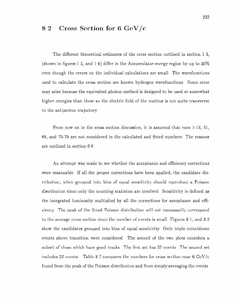
232
8.2 Cross Section for 6 GeV/c
The di�erent theoretical estimates of the cross section outlined in section 1.3,
(shown in �gures 1.5, and 1.6) di�er in the Accumulator energy region by up to 30%
even though the errors on the individual calculations are small. The wavefunctions
used to calculate the cross section are known hydrogen wavefunctions. Some error
may arise because the equivalent photon method is designed to be used at somewhat
higher energies than these so the electric �eld of the nucleus is not quite transverse
to the antiproton trajectory.
From now on in the cross section discussion, it is assumed that runs 1-13, 51,
68, and 75-79 are not considered in the calculated and �tted numbers. The reasons
are outlined in section 6.6.
An attempt was made to see whether the acceptance and e�ciency corrections
were reasonable. If all the proper corrections have been applied, the candidate dis-
tribution, when grouped into bins of equal sensitivity should reproduce a Poisson
distribution since only the counting statistics are involved. Sensitivity is de�ned as
the integrated luminosity multiplied by all the corrections for acceptance and e�-
ciency. The peak of the �tted Poisson distribution will not neccessarily correspond
to the average cross section since the number of events is small. Figures 8.1, and 8.2
show the candidates grouped into bins of equal sensitivity. Only triple coincidence
events above transition were considered. The second of the two plots considers a
subset of these which have good tracks. The �rst set has 57 events. The second set
includes 52 events. Table 8.7 compares the numbers for cross section near 6 GeV/c
found from the peak of the Poisson distribution and from simply averaging the events.

233
Figure 8.1: Number of events in equal sensitivity bins. All triple coincidences areconsidered. The curve shown is a Poisson distribution �tted to the data.
Table 8.7: Comparison of cross section (pb�1) estimates.
No cuts Good Track only
Binned 0.979 1.09
Average 1.129 1.03

234
Figure 8.2: Number of events in equal sensitivity bins. Only triple coincidences witha good track are considered. The curve shown is a Poisson disttribution �tted to thedata.

235
A maximum likelihood �t was made to the data by assuming the number of
candidate events followed a Poisson distribution. The expected mean of the Poisson
distribution was set equal to the product of the integrated luminosity � corrections
� expected cross section:
�i = (ZLdt)i � �i � �exp(P�p;i) (8.1)
Each run-momentum combination was used separately as a datum point. Triple
coincidence data and foil-out data were �tted separately. For each, �ts were made
with both above and below transition data, and with above transition data only.
For the expected cross section as a function of momentum, the form derived
by Munger, Brodsky, and Schmidt[47] was used. The constant multiplier which they
calculated to be f = 1:42 was allowed to be a freely adjustable parameter in the �t.
The function of momenta comes purely from the equivalent photon method.
�exp(P�p; i) = f � (ln( 2 + 1)� 2
( 2 + 1)); =
qP 2�p;i +m2
�p (8.2)
The maximum likelihood function is a product of N Poisson functions,
� =NYi=1
�nii e��i
ni!(8.3)
where ni is the number of events observed for the ith datum point. The log-likelihood
function, -ln(�), is maximized resulting in �tted values for the factor, f . Table 8.8
shows the resulting values for f and the corresponding cross section at 6 GeV/c.

236
Table 8.8: Results of maximum likelihood �ts. Cross section is in pb. �Mean =�8�1=
p8
f �(P = 6 GeV=c)
Foil-in 0:4215+0:0803�0:0712 1:1727+0:223�0:198
Foil-in, good track only 0:4080+0:0790�0:0700 1:1351+0:220�0:195
Foil-in, above transition 0:4241+0:0838�0:0739 1:1798+0:233�0:206
Foil-in, above transition, 0:4169+0:0831�0:0733 1:1597+0:231�0:204
good track only
Foil-in, above transition, 0:3852+0:0841�0:0734 1:0717+0:234�0:204
runs 52-74 removed
Foil-in, above transition, 0:3773+0:0832�0:0726 1:0496+0:231�0:202
runs 52-74 removed
good track only
Foil-out 0:4089+0:1327�0:1090 1:1374+0:369�0:303
Foil-out, above transition 0:4256+0:1492�0:1207 1:1840+0:415�0:336
Mean��Mean 1.1363 � 0.018

237
Figure 8.3: Maximum likelihood function (unnormalized), -ln(�), as a function of theunknown factor, f . Events are foil-out only.
Figures 8.3, 8.4, 8.5, 8.6, and 8.7 show the maximum likelihood function result-
ing. The values listed are the location, f , of the peak.
8.3 Energy Dependence of the Cross Section
Figure 8.8 shows the events per luminosity displayed as a function of beam
momentum. No corrections have been made to the data. Figures 8.9, and 8.10
show the cross section which is the events per luminosity with corrections taken into
account.
Figure 8.11 shows the expected functions for the theoretically predicted an-
tihydrogen production cross section from theory and measured data binned where
measurements have been binned together in bins of momentum to increase statistics
of the bins. The cross section measured by PS210 at 1.94 GeV/c is calculated from

238
Figure 8.4: Maximum likelihood function (unnormalized), -ln(�), as a function of theunknown factor, f . Events are foil-in. above transition only.
Figure 8.5: Maximum likelihood function (unnormalized), -ln(�), as a function of theunknown factor, f . Events are foil-in, above transition only, with certain runs notconsidered.

239
Figure 8.6: Maximum likelihood function (unnormalized), -ln(�), as a function of theunknown factor, f . Events are foil-out only.
Figure 8.7: Maximum likelihood function (unnormalized), -ln(�), as a function of theunknown factor, f . Events are foil-out, above transition only.

240
Figure 8.8: Events per luminosity using 10 bins in momentum.

241
Figure 8.9: Cross section using 10 bins in momentum. The line represents a �2 �t toF( ) from [47].

242
Figure 8.10: Cross section using 25 bins in momentum. The line represents a �2 �tto F( ) from [47].

243
the values given in [5]. Namely, 11 candidate events were observed. Two were de-
termined to be background. The rest were assumed to be antihydrogens. With the
statistical error and error on integrated luminosity, their cross section measurement
normalized from xenon (Z = 54) to hydrogen is:
�(PS210; P�p = 1:94GeV=c) = 2:058 �1:029 �0:686pb (8.4)
The PS210 result agrees with the theory quite well considering the large error bars.
There is still a question to be answered as to why E862's measured cross section is
consistently lower than expectations. The luminosity integrated by E862 is known
very well so either the antihydrogen cross section has a di�erent dependence than
predicted or some unknown acceptance problem was encountered.

244
Figure 8.11: Antihydrogen production cross section. Curves are theoretical functionsfrom (MBS)[47], (Baur)[48], (BB 97)[57], and (Eichler)[63]. Data points are from [5]and the present results [93].

245
8.4 Systematic Errors
The systematic errors in the cross section measurement arise because of impre-
cise knowledge of the integrated luminosity (4% mostly from the error on the active
area of the detector) and and from assumptions on the acceptance calculation. The
systematic error in the acceptance estimate is dominated by how well the emittance,
and hence the beam size, is known. Another smaller e�ect is the position of the target
wheel. We allowed a possible 2o rotation since the video camera, which monitored the
optical readout of the wheel's angle setting, provided a resolution no better than 2o.
Such e�ects as a possible, small momentum scale error or error in the track's recon-
structed position at the jet, etc. had no e�ect on the cross section since no candidates
as chosen by the fundamental signatures, (triple coincidence or track with spectator
hit in PWC #1), had a momentum or position at the jet far signi�cantly outside the
accceptable range. The error arising from Monte Carlo statistics was small (< 2%).
The systematic change to the acceptance � e�ciency was calculated by running the
simulations described in chapter 7 with the assumed o�sets. The assumed o�sets
were a 2o change in target wheel angle and a 50% increase in emittance envelopes in
both x and y dimensions. Possible beam position measurement error is comparably
small. This amounted to a roughly 10% change in the cross section. One e�ect which
was di�cult to model was the correct positions of the e+ spectrometer magnets. The
magnets had been moved signi�cantly from their original, ideal positions. On the
other hand, they were moved to correct for imperfections in the construction of the
magnets themselves. Thus the empirical success in pointing the test beam of e�
on the scintillator, as described in chapter 3, shows that the acceptance of the e+
spectrometer cannot be much di�erent than the ideal scenario.

246
Table 8.9: Cross section results for di�erent foil thicknesses. The data sets chosenwere slightly di�erent than that used in the previous analysis.
Data Number Integ. Cross Stat. Syst.Set of Lumin. Section Error Error
Events (pb�1) (pb) (pb) (pb)437 �g/cm2 foil 24 34.8 1.03 0.21 0.08777 �g/cm2 foil 33 29.6 1.22 0.21 0.09
No foil 10 11.3 1.08 0.35 0.12All data 67 75.7 1.12 0.14 0.09
The e�ect of the combined error from the integrated luminosity and acceptance
are included in table where the cross section is calculated for a somewhat di�erent
breakup of the data as outlined in [93].

247
8.5 Conclusions
In conclusion, antihydrogen atoms have unquestionably been observed. Two
di�erent signatures have signalled the antihydrogen, one with the foil target in place,
(triple coincidence events), and the other with the foil out of the way (high momentum
with spectator hit events). Both types of events prove completely consistent with the
antihydrogen hypothesis when each of the kinematic distributions are viewed. A
cross section measurement has been made for those events around 6 GeV/c where
there is a large number of events. The cross section is for antihydrogen production
at P�p = 5:767 GeV/c, � = 1:14 pb. The cross section does not agree with the
theoretical cross section for this momentum (� =� 3:8 pb) [47]. A measurement
of the energy dependence of the cross section has been made although, because of
much lower statistics at the extreme beam momenta of the range available (3 - 9
GeV/c), agreement with the form of the theoretical cross section is consistent but
not de�nitive. A monotonic function increasing with momentum is clear though.
The results presented here are in partial agreement with the results of CERN
PS210[5], (see section 1.4). The observation of antihydrogen has been made at similar,
although larger, momenta. The signature of the events is similar. Certain advantages
of E862 are the better antiproton momentum resolution, further separation of the e+
spectrometer from the antiproton beamline, much further removal of the apparatus
from backgrounds, and measurement ability over a range of beam momenta.
These achievements would not have been possible without recognizing the con-
tinually improving ability to collect and cool antiprotons over the past 20 years. The
progress of the antiproton storage rings at Fermilab and CERN has allowed stacks
of greater than 1011�p to be collected for experimental study. Even so, a rate of only
one or two antihydrogens per day could be measured. A higher production rate will

248
be required to study the system with any precision. The technology of thin gas jets
is also needed in order to insure the beam can recirculate but still produce enough
antihydrogen to be measured.
It is true that other production approaches should come to fruition soon, their
advantages being larger formation rates and ability to perform much more precise
spectroscopy on the atomic system. On the other hand, as outlined in Appendix 2, we
can perform atomic spectroscopy with higher energy antihydrogen as well. The Lamb
shift splitting can be directly measured as a way to probe for CPT-violating inter-
actions. If they exist, they could ultimately alter our understanding of the Standard
Model of particle physics.

Bibliography
[1] Dirac, P.A.M., 1928, Proc. Roy. Soc., A117, 610.
[2] Dirac, P.A.M., 1931, Proc. Roy. Soc., A133, 60.
[3] Anderson, C.D., Phys. Rev., 43, 491, 1932; Science, 76, 238, 1932.
[4] Chamberlain, O., Segre, E., Wiegand, C., Ysilantis, T., Phys. Rev., 100, 947,
1955.
[5] G. Baur et al., Production of Anti-Hydrogen, Phys. Lett., B 368, 251, 1996.
[6] G. Luders, Det. Kon. Dan. Vid. Sel. Mat.-fys Medd., 28, 5, 1954.; G. Luders,
Ann. Phys., 2, 1957.
[7] W. Pauli, in: Niels Bohr and the development of physics, ed. W. Pauli
(Pergamon, New York), 30, 1955.
[8] J.S. Bell, Proc. Roy. Soc., A 231, 479, 1955.
[9] R. Jost, The general theory of quantized �elds, (American Mathematical Society,
Providence, Rhode Island), 1965.
[10] D. Colladay and V.A. Kostelecky, CPT violation and the standard model, Phys.
Rev., D 55, 11, 1997.
[11] J. Ellis, N.E. Mavromatos, and D.V. Nanopoulos, CPT violation in string-
modi�ed quantum mechanics and the neutral kaon system, Int. J. Mod. Phys.,
A 11, 1489, 1996.
249

250
[12] S. Hawking, The unpredictability of quantum gravity, Commun. Math. Phys.,
87, 395, 1982.
[13] Review of Particle Properties, Particle Data Group, Phys. Rev., D50, 3, 1994.
[14] G.D. Gollin and W.P. Hogan, New Measurements of CP violation parameters as
tests of CPT in K meson decay, Proceedings of the 27th International Conference
on High Energy Physics, Glasgow, 1994.
[15] G.B. Thomson et al., An experiment studying KL�KS interference to test CPT
conservation at the Planck scale, Rutgers preprint RU-96-82.
[16] I.N. Meshkov, Experimental Studies of antihydrogen and positronium physics:
Problems and possibilities, Phys. Part. Nucl., 28, 2, 1997.
[17] T.Kinoshita, The �ne structure constant, Rep. Prog. Phys., 59, 1459, 1996.
[18] G.W. Erickson and D.R. Yennie, Part I, Ann. Phys., 35, 271, 1965.
[19] G.W. Erickson, Improved Lamb-Shift Calculation for All Values of Z, Phys. Rev.
Lett., 27, 12, 1971.
[20] P. Mohr, Lamb Shift in a Strong Coulomb Potential, Phys. Rev. Lett., 34, 16,
1975.
[21] S.G. Karshenboim, The lamb shift in the hydrogen atom, JETP, 79, 2, 1994.
[22] R.T. Robiscoe and T.W. Shyn, Phys. Rev. Lett., 24, 559, 1970.
[23] S.R. Lundeen and F.M. Pipkin, Phys. Rev. Lett., 46, 232, 1981.
[24] S.R. Lundeen, Bull. Amer. Phys. Soc., 20, 11, 1975.
[25] V.G. Pal'chickov, Y.L.Sokolov, and V.P.Yakovlev, Pis'ma Zh. Eksp. Teor. Fiz.,
38, 347, 1983 [JETP Lett., 38, 418, 1983].

251
[26] Y.L. Sokolov and V.P.Yakovlev, Measurement of the Lamb shift in the hydrogen
atom (n=2), Sov. Phys. JETP., 56, 1, 1982.
[27] D.A. Andrews and G. Newton, Radio-Frequency Atomic Beam Measurement of
the (22S1=2; F = 0) � (22P1=2; F = 1) Lamb-Shift Interval in Hydrogen, Phys.
Rev. Lett., 37, 19, 1976.
[28] E.W. Hagley and F.M. Pipkin, Separated Oscillatory Field Measurement of
Hydrogen 2S1=2 � 2P3=2 Fine Structure Interval, Phys. Rev. Lett., 72, 8, 1994.
[29] The Production and Study of Cold Antihydrogen, by the Antihydrogen TRAP
Collaboration, G.Gabrielse et al., CERN-SPSLC 96-23/I211, 1996.
[30] Progress report on the design of the ATHENA apparatus, the ATHENA
Collaboration, CERN-SPSC 97-9, SPSC/M597, 1997.
[31] D.J. Berkeland et al., Precise optical measurement of Lamb shifts in atomic
hydrogen, Phys. Rev. Lett., 75, 13, 1995.
[32] S. Bourzeix et al., High resolution spectroscopy of the hydrogen atom:
Determination of the 1S Lamb shift, Phys. Rev. Lett., 76, 3, 1996.
[33] S. Klarsfeld and A. Maquet, Bethe sums for Lamb shift calculations in higher
excited states, Phys. Lett. B, 43, 3, 1973.
[34] S. Brodsky and R. Parsons, Precise Theory of the Zeeman Spectrum for Atomic
Hydrogen and Deuterium and the Lamb Shift, Phys. Rev., 163, 1, 1967.
[35] M. Charlton et al, Antihydrogen Physics, Phys. Rep., 241, 65, 1994.
[36] L. Brown and G.Gabrielse, Geonium Theory: Physics of a single electron or ion
in a Penning trap, Rev. Mod. Phys., 58, 1986.
[37] W. Quint et al., (Anti)hydrogen recombination studies in a nested Penning trap,
Hyper�ne Interactions, 76, No. 1-4, 181, 1993.

252
[38] F.B. Yousif et al., Phys. Rev. Lett., 67, 26, 1991.
[39] H. Bethe and E. Salpeter, Quantum Mechanics of One- and Two-Electron Atoms,
Springer-Verlag, Berlin, 1957.
[40] Bertulani and Baur, Electromagnetic Processes in Heavy Ion Collisions, Phys.
Rep., 193, 398, 1990.
[41] G.I. Budker and A.N. Shrinsky, Usp. Fiz. Nauk., 124, 561, 1978; [Sov. Phys.
Usp., 21, 277, 1978]; M. Bell et al., Nucl. Inst.& Meth., 190, 237, 1981; H. Poth
et al., Z. Phys. A., 332, 171, 1989.
[42] U. Schramm et al., Phys. Rev. Lett., 67, 22, 1991.
[43] A. Wolf, Laser Stimulated Formation and Stabilization of Antihydrogen Atoms,
Hyper�ne Interactions, 76, No. 1-4, 189, 1993.
[44] B. Deutch et al., Antihydrogen synthesis by the reaction of antiprotons with
excited state positronium atoms, Hyper�ne Interactions, 76, No. 1-4, 153, 1993.
[45] Y. Ito et al., Possible formation of antihydrogen atoms from metastable antipro-
tonic helium atoms and positrons/positronium, Hyper�ne Interactions, 76, No.
1-4, 163, 1993.
[46] M. Iwasaki et al., Phys. Rev. Lett., 67, 1246, 1991.
[47] C.Munger, S.Brodsky, I.Schmidt, Production of relativistic antihydrogen atoms
by pair production with positron capture, Phys. Rev., D 49, 7, 1994.
[48] G. Baur, Photon-photon and bremsstrahlung production of fast antihydrogen in
�p-nucleus collisions, Phys. Lett., B 311, 343, 1993.
[49] C.Munger, S.Brodsky, I.Schmidt, Production of relativistic antihydrogen atoms
by pair production with positron capture and measurement of the Lamb shift,
Hyper�ne Interactions, 76, 175, 1993.

253
[50] S. Brodsky and A.H. Mueller, Using Nuclei to Probe Hadronization in QCD.,
Phys. Lett., B 206, 4, 1988.
[51] S.J. Brodsky, J.F. Gunion, and D.E. Soper, Physics of heavy-quark production
in quantum chromodynamics, Phys. Rev., D 36, 9, 1987.
[52] R. Vogt, S.J. Brodsky, and P. Hoyer, Systematics of J/ Production in Nuclear
Collisions, Nucl. Phys., B 360, 67, 1991.
[53] G. Baur and Bertulani, C.A., Electromagnetic physics at relativistic heavy ion
colliders, for better of for worse, Nucl. Phys., A 505, 835, 1989.
[54] D. Perkins, Introduction to High Energy Physics, third edition, Addison Wesley
Publishing Company, Inc., 1987.
[55] G. Baym, Lectures on Quantum Mechanics, 173, Addison-Wesley Publishing
Company, Redwood City, CA., 1969.
[56] V.M. Budnev et al., The Two-Photon Particle Production Mechanism.
Equivalent Photon Approximation., Phys. Rep., C 15, 4, 1975.
[57] C.A. Bertulani and G. Baur, Antihydrogen production and accuracy of the
equivalent approximation, HEP-PH/9711273v1 preprint from LANL xxx archive,
1997; submitted to Phys. Rev. D.
[58] M.J. Rhoades-Brown, C. Bottcher, M.R. Strayer, Feynman-Monte Carlo calcu-
lations of electron capture at relativistic energies, Phys. Rev., A 40, No. 5, 2831,
1989.
[59] A.J. Baltz, M.J. Rhoades-Brown, and J. Weneser, Energy Dependence of Bound
Electron-Positron Pair Production at Very High Energy Ion-Ion Transits, Phys.
Rev., A 44, No. 9, 5569, 1991.

254
[60] A. Aste, K. Hencken, D. Trautmann, G. Baur, Electromagnetic pair production
with capture, Phys. Rev., A 50, No. 5, 3980, 1994.
[61] U. Becker, Distribution of positrons emitted from pair production with capture
in relativistic heavy ion collisions, J. Phys. B, 20, 6563, 1987.
[62] C.A. Bertulani and G. Baur, Electromagnetic Processes in Relativistic Heavy
Ion Collisions, Nucl. Phys., A 458, 725, 1986.
[63] J. Eichler, Charge Transfer from the Negative Energy Continuum: Alternative
Mechanism for Pair Production in Relativistic Atomic Collisions, Phys. Rev.
Lett., 75, 20, 1995.
[64] A. Belkacem, et al., Projectile Energy and Atomic Number Dependence of
Electron Capture from Pair Production in Relativistic Heavy Ion Collisions,
Phys. Rev. Lett., 73, No. 18, 2432, 1994.
[65] A. Belkacem, et al., Measurement of Electron Capture from Electron-Positron
Pair Production in Relativistic Heavy Ion Collisions, Phys. Rev. Lett., 71, 10,
1993.
[66] Boero et al., The internal Xe-jet target for the formation of antihydrogen atoms
at CERN LEAR, CERN PPE/96-105, 1996, published in Nuovo Cimento A.
[67] Design Report: Tevatron 1 Project, Fermi National Accelerator Laboratory.
Batavia, IL, (unpublished), September 1984.
[68] J.Peoples et al., The FermilabAntiproton Source, IEEE Trans. Nucl. Sci., NS-30,
1970, 1983.
[69] E760 Collaboration, Measurement of the J= and 0 resonance parameters in �pp
annihilation, Phys. Rev., D 47, 3, 1993.
[70] M. Macri, Gas Jet Targets, CERN Accelerator School 1983, CERN 84-15, 1984.

255
[71] FNAL P835, Proposal to continue the study of charmonium spectroscopy in �p�pcollisions, 1993.
[72] D. Allspach et al., Refrigerated Hydrogen Gas jet for the Fermilab Antiproton
Accumulator, Proceedings of the Cryogenic Engineering Conference, Columbus
Ohio, July 17-21, 1995.
[73] A.Cecucci et al., Charmonium Formation in P Anti-P Annihilation by
Experiment E760, Nucl. Phys., A 558, 259c, 1993.
[74] S. Trokenheim et al., A p�p luminosity monitor for Fermilab experiment E760,
Nucl. Inst. & Meth., A 355, 308, 1995.
[75] M.K. Prasad, Acta Physica Polonica, B 10, 635, 1979.
[76] M.S. Gulley et al, Measurement of H�;Ho, and H+ cross sections produced by
foilstripping of 800 MeV H� ions, Phys. Rev., A 53, 3201, 1996.
[77] R.C. Webber and C. Hojvat, Measurement of the Electron Loss for Negative
Hydrogen Ions on Carbon at 200 MeV., IEEE Trans. Nucl. Sci., NS-26, 3, 4012,
1979.
[78] E. Acerbi et al., Lett. Nuov. Cim., 10, No. 14, 598, 1974.
[79] P.B. Keating et al., Electric-�eld-induced electron detachment of 800-MeV H�
ions, Phys. Rev., A 52, 4547, 1995.
[80] C. Hojvat, M. Joy, and, R.C. Webber, Stripping Foils for Multiturn Charge
Exchange Injection into the Fermilab Booster, IEEE Trans. Nucl. Sci., NS-26,
3, 4009, 1979.
[81] D.A. Edwards and M.J. Syphers, An Introduction to the Physics of High Energy
Accelerators, John Wiley and Sons, Inc., New York, NY, 1993.

256
[82] D.B. Montgomery, Solenoid Magnet Design (The Magnetic and Mechanical
Aspects of Resistive and Superconducting Systems), John Wiley and Sons, New
York, NY, 1969.
[83] S. Humphries, Charged Particle Accelerators, John Wiley and Sons, New York,
NY, 1900.
[84] P.A.M. Dirac, P.A.M., Proc. Camb. Phil. Soc., 26, 361, 1930.
[85] W. Heitler,The Quantum Theory of Radiation, Oxford University Press, London,
1954.
[86] H.W. Kendall and M. Deutsch, Annihilation of Positrons in Flight, Phys. Rev.,
101, 1, 1996.
[87] W.R. Leo, Techniques for Nuclear and Particle Physics Experiments, Springer-
Verlag, 1987.
[88] D.C. Christian et al., High Rate Drift Chambers, Nucl. Inst. & Meth., A 345,
62, 1994.
[89] G.L. Kane and A. Seidl, Two-body hadron reactions, Rev. Mod. Phys., 48, 2, 1,
1976.
[90] FNAL P862, Proposal for the detection of relativistic antihydrogen atoms pro-
duced by pair production with positron capture, 1992.
[91] D.M. Ritson, Techniques of High Energy Physics, Interscience Publishers, Inc.,
New York, 16, 1961.
[92] W. Nelson, et al., The EGS4 Code System, SLAC-Report-265, 1985.
[93] G.Blanford et al., (Fermilab E862 Collaboration), Observation of Atomic
Antihydrogen, submitted to Phys. Rev. Lett.

257
[94] V.B. Berestetskii, E.M. Lifshitz, L.P. Pitaevskii, Quantum Electrodynamics,
Pergamon Press, 1982. (from Landau and Lifshitz Theoretical Physics series).
[95] M.Mandelkern et al.(Fermilab E862 Collaboration), Letter of intent for a con-
tinuation of E862: Measuring the Lamb shift and �ne structure of antihydrogen,
(unpublished).
[96] R.J. Damburg, V.V. Kolosov, A hydrogen atom in a uniform electric �eld III, J.
Phys., B 12, 16, 1979.
[97] T. Yamabe, A. Tachibana, H. Silverstone, Theory of the ionization of the hydro-
gen atom by an external electrostatic �eld, Phys. Rev., A 16, 3, 1977.
[98] W.E. Lamb,Jr., and R.C. Retherford, Phys. Rev., 60, 817, 1941.
[99] V.V. Parkhomchuk, Measurements of the Lamb shift in a relativistic hydrogen
atom, Hyper�ne Interactions, 44, 315, 1988.
[100] R. Neumann, Fast antihydrogen beam spectroscopy, Hyper�ne Interactions, 44,
305, 1988.
[101] G.Blanford et al., (Fermilab E862 Collaboration), Measuring the Antihydrogen
Lamb Shift with a Relativistic Antihydrogen Beam, submitted to Phys. Rev. D.

Appendix A
Relativistic Cross Section
Calculation
This appendix is an attempt to bring together the parts of the calculation
needed for the antihydrogen production cross section. The material, adapted from
references [94], [47], [85] is not original and is solely intended to condense the material
into a readable review format.
A.1 Photoelectric Matrix Element
The antihydrogen production reaction observed by E862 is based on an antipro-
ton passing near a proton close enough to interact with the proton's electromagnetic
near �eld and produce an e+ � e� pair. The proton's �eld can be fourier analyzed
into a spectrum of virtual photons. The Weizs�acher-Williams method of virtual pho-
tons is used to express the virtual photon spectrum as a spectrum of real photons.
This is possible because the antiproton's large relativistic boost makes the near �eld
look nearly transverse to the antiproton. Now one can consider the interaction of the
antiproton with a single real photon which results in an electron and a bound antihy-
drogen. One of the insights found in [47] was to change this photon induced capture
reaction into the photoelectric reaction by using crossing symmetry (s$ u). So the

259
�rst step is to calculate the photoelectric matrix element. After crossing symmetry is
invoked, the Weizs�acher-Williams method is used to do the sum over photons in the
proton's near �eld.
For the photoelectric process, the choice of wavefunctions for the initial atom
and �nal electron is important.
Mpe(k) = f < ~jfi � ~A > i =Zd3x 0
f�(~� � ~e)ei~k�~r i (A.1)
The e�ect of the Coulomb force on both the incoming and outgoing electron
(plane wave) is viewed as a perturbation. The initial state wave function is basically
a relativistic modi�cation to the non-relativistic hydrogen wave function.
Potential energy : U = �Z�=r (A.2)
In order to get the perturbation wave function, The Dirac equation, (E � U �m� + i~� � ~r) = 0, can be multiplied by its complex conjugate to get a 2nd order
equation, where ~�; � are the spin matrices formed from the Dirac matrices,
(E � U +m� � i~� � ~r)(E � U �m� + i~� � ~r) = 0, or (A.3)
(� + p2 � 2EU) = (�i~� � ~rU � U2) (A.4)

260
The �nal state wave function of the electron is a sum of plane wave and a
perturbation part.
f =1p2E
[u0ei~p�~r + (1)] (A.5)
i = u non�rel + (1) = [1� i
2m o(~ � ~r)] up
2m non�rel; (A.6)
non�rel =(Ze2m)3=2p
�e�Ze
2mr = Ro � Yoo (A.7)
where u = spinor part.
The initial state wavefunction is a bound state but has this relativistic modi�-
cation.
(E2 �m2) + U2 � 2EU + (~�2 = 1) � (~r � ~r) = p2 + U2 � 2EU +� (A.8)
and using,
f�; ~�g = �~�+ ~�� = 0 (A.9)
and integrating by parts,
(� + p2 + U2 � i~� � ~rU � 2EU) = 0 (A.10)
(1
2m�� j�nj+ Z�
r) (1) =
iZ�
2m(~r1
r) � (~�u) non�rel + ::: (A.11)

261
(� + p2 � 2EU)( = u non�rel + (1)) = (�i~� � (~rU)� U2)( = u non�rel + (1))
(A.12)
Using,
p2
2m= �j�nj � U (A.13)
and rejecting terms of order (Z�)2,
(1) = � i
2m(~�u) � ~r non�rel (A.14)
Finally with this choice of wave functions, the matrix element becomes
Mfi =1p2m
1p2E
�Zd3x�u0(~ � ~e) � [1� i
2m o(~ � ~r)] � (A.15)
�u non�rel � e�i(~p�~k)�~r + � (1)(~ � ~e)ei~k�~ru non�rel (A.16)
Now integrate by parts (using the surface boundary condition,
RS @(d
3x)u non�rele�i(~p�~k)�~r = 0 where S is sphere with r!1),
Z(�~r)u non�rele�i(~p�~k)�~rd3x (A.17)
Mfi =(Ze2m)3=2
2p�mE
�u0(~ � ~e)[1 + 1
2m o~ � (~p�~k)]uF(~p�~k)(e�Ze
2mr) + � (1)
�~k(~ � ~e)u (A.18)
where the non-relativistic wave function has been replaced by a constant but
only in the last term (not inside the derivative).

262
The Fourier transforms needed are,
F(~p�~k)(e�Ze2mr) =
8�Ze2m
(~p � ~k)4 ; (A.19)
F(~p�~k)(1=r) =4�
(~k � ~p)2(A.20)
To calculate � (1)
�~k, the Dirac equation is used,

263
( oE + i~ � ~r�m) (1) = e(~ �A�)u0eip�~r = �Ze
2
r ou0eip�~r (A.21)
and
Z( oE + i~ � ~r+m)( oE + i~ � ~r�m) (1)e�i
~k�~rd3x (A.22)
= �Ze2Z( oE + i~ � ~r+m) ou0
1
reip�~re�i
~k�~rd3x (A.23)
=Z(� + p2) (1)e�i
~k�~rd3x (A.24)
using o; ~ = 0 and a parts integration,
~ �Z~r1
rei(~p�
~k)�~rd3x = �~ � F(~k�~p)(1
r)(�1)(�k)ei(~p�~k)�~r (A.25)
Z� (1)e�ik�~rd3x = �k2 (1)
~k(A.26)
(p2 � k2) (1)k = �Ze2
Z[2E o + ~ � (~p � ~k)]F(~k�~p)(
1
r)ei(~p�
~k)�~r ou0d3x (A.27)
using m = ( oE + ~p � ~ ) ou0,
Resulting in:
� (1)
�~k= [
4�
(~k � ~p)2Ze2
(k2 � p2)�u0(2E o + ~ � (~k � ~p))] o (A.28)

264
Mfi =(Ze2m)3=2
2p�mE
�u0[1 +1
2m o~ � (~p � ~k)] � u8�Ze
2m
(~p� ~k)4 (A.29)
+4�Ze2�u02E o + ~ � (~k � ~p)
(k2 � p2)(~k � ~p)2� o(~ � ~e)u (A.30)
Mfi =4�(Ze2m)5=2pmE(~k � ~p)2
�u0Au (A.31)
A = a(~ � ~e) + (~ � ~e) o(~ �~b) + (~ � ~c) o(~ � ~e) (A.32)
a � 1
(~k � ~p)2+E
m
1
k2 � p2(A.33)
~b � �(~k � ~p)
2m(~k � ~p)2(A.34)
~c � �(~k � ~p)
2m(k2 � p2)(A.35)
(A.36)
The photoelectric matrix element can now be written more compactly using the
matrix A de�ned in [94] and its Hermitian conjugate, Ay:
jMfij2pe =16�(Ze2m)5
m"(~k � ~p)4(�u0Au)(�u �Au0); �A � oAy o (A.37)
d� =8e2(Ze2m)5
!(~k � ~p)4j~pjm(�u0Au�u �Au0)d (A.38)
d� =1
2e2�j~pjjMfij2d (A.39)

265
16e2(Ze2m)5j~pjm!(~k � ~p)4
Tr(�0A� �A)d (A.40)
where � is the initial polarization matrix, �0 is the �nal state polarization matrix,
the �rst averaged, the second summed over spin directions.
� =1
2m( o + 1) =
1
2( � p +m) (A.41)
�0 =1
2( o"� ~ � ~p+m) =
1
2( � p+m)(1� 5~ � ~g) (A.42)
where ~g is the spin in the rest frame.
~ y = �~ ; oy = o; f o; ~ g � o~ + ~ o = 0 (A.43)
Tr(�0A� �A) = Tr�1
2( o"� ~ � ~p+m)
ha(~ � ~e) + (~ � ~e) o(~ �~b) + (A.44)
(~ � ~c) o(~ � ~e)i� 1
2m( o + 1)
ha o(~ � ~e)y o + (A.45)
of(~ � ~e) o(~ �~b)gy o + of(~ � ~c) o(~ � ~e)gy oi�
(A.46)
Using,
1
4Tr�( ~A � ~ )( ~B � ~ )
�= � ~A � ~B (A.47)
1
4Tr�( ~A � ~ )( ~B � ~ )(~C � ~ )( ~D � ~ )
�= (A.48)
= ( ~A � ~B)(~C � ~D)� ( ~A � ~C)( ~B � ~D) + ( ~A � ~D)( ~B � ~C) (A.49)

266
After three pages of algebra,
Tr(�0A� �A) =m
"+m
ha~p� (~b�~c)("+m)
i2+4m(~b �~e)
h("+m)(~c �~e)+a(~p �~e)
i(A.50)
~e is real and linear-polarized. (e = e�)
Tr(�0A� �A) =m
"+m
�a2(~p � ~p)� 2a~p � (~b� ~c)("+m) + (A.51)
+(b2 + c2 � 2~b � ~c("+m)2)�
(A.52)
+4m(~b � ~e)("+m)(~c � ~e) + 4m(~b � ~e)a(~p � ~e) (A.53)
Now let's assume a right-handed, spherical coordinate system:
(~k � ~p)2 = k2p2cos2� (A.54)
(~p � e)2 = p2sin2�cos2� (A.55)
(~k � e) = 0 (A.56)
Tr(�0A� �A) =�a2p2m
"+m+ a(~k � ~p � p2)(
1
k2 � p2� 1
(~k � ~p)2) (A.57)
+"+m
4m(~k � ~p)2(
1
k2 � p2� 1
(~k � ~p)2)2 (A.58)
�"+m
2m
k2p2 � (~k � ~p)2(k2 � p2)(~k � ~p)2k2
+ ak2p2 � (~k � ~p)2(~k � ~p)2k2
�(A.59)
jM j2photo =(32�)2�6m4M2
(~k � ~p)4Tr(�0A� �A) (A.60)

267
A.2 Cross Section Integration
The next step is to express the kinematic variables of the photoionization process
in terms of the Mandelstam variables. We need k2; p2; and ~k � ~p as functions of s,t,u.Notice that if one switches the de�nitions of t and u, the variables represent instead the
capture process. Assume m = electron mass and M = proton mass. " =qj~pj2 +m2.
s =M2 + 2M! (A.61)
t =M2 � 2"M +m2 (A.62)
u = m2 � 2!" + 2~k � ~p (A.63)
k2(s) = !2 =�s�M2
2M
�2(A.64)
(~k � ~p)(s; t; u) = t�m2
2+�s�M2
2M
��M2 +m2 � u
2M
�(A.65)
p2(u) =�M2 +m2 � u
2M
��m2 (A.66)
Now we would like the capture cross section, of course, so we use the crossing
symmetry by switching the variables: (s $ t). Notice in Munger, Brodsky, and
Schmidt [47], they use the Mandelstam variables for the capture process instead but
interchange s$ u. This turns out to yield the same cross section. An equivalent way
of doing the transformation is not to use the Mandelstam variables at all but simply
to switch the sign of the electron energy �$ ��. To reiterate the de�nitions shown

268
in section 1.3 originally from [47],
�
�� �� =
Z M�p
2me
d!
!� �p! �H(1S)e�(!) (A.67)
� ��p!e� �H(1S)(!) =p
64�2!M2
ZjM j2capturede (A.68)
The ratio of �� (resulting from the s $ t) to �� (from the � ! � method) is shown
in �gure A.1 along with the individual cross section estimates found by integrating
equation A.59. The horizontal axis is the upper limit of the photon energy integration
in units of the electron mass. The upper limits for the integrations over transverse
momentum transfer, q2?, and over photon energy, !, are important choices. The
suggestion from [47] is to integrate up to q2? = !2 and then integrate ! up toMp� =5500 � 2me at 6 GeV/c, for example.

269
Figure A.1: Results of integrating capture cross section formula shown in equationA.59, (derived in[47]), using two di�erent transformations for the crossing symmetry.

Appendix B
Spectroscopy of Relativistic �H
B.1 Goals
In order to explore the possibility of a CPT symmetry violation in the hydrogen-
antihydrogen system, the energy levels of antihydrogen atoms need to be measured
precisely and compared to those of hydrogen atoms. Antihydrogen atoms produced
with the technique described in this dissertation, besides having a small production
rate, are characterized by large energy spreads making it di�cult to precisely measure
the energy spectrum. One can partially circumvent this by designing an experiment
which exploits the interference of a two level quantum system. The level splittings
are really what we want to measure in order to learn about the interactions of the
constituent particles as opposed to the individual particle masses. An overall, uniform
shift of all of the antihydrogen energy levels with respect to those of hydrogen would
be missed using this method.
I will outline, in the subsequent chapter, plans for measuring the �ne structure
and Lamb shift splittings of the n=2 level using an interference method by extending
the present experiment. A discussion of similar methods is given in [16]. The �rst
270

271
step is to increase the production rate in order to make higher statistics spectroscopic
measurements. Next, it will be shown that antihydrogen n > 1 states can be produced
(with an excitation foil) and measured as distinct from the n = 1 states. Finally,
methods of exciting the 2S1=2� 2P1=2 transition and measuring the energy di�erence
are discussed. A more detailed description is found in [95].
B.2 Unperturbed Spectrum
The unperturbed spectrum of the hydrogen atom is shown in �gure B.1. A
hierarchy of three types of energy splittings dominate the corrections to the �1=n2
energy dependence of the Bohr levels. These are the spin-orbit, Lamb shift, and
hyper�ne corrections. The 2P1=2 and 2P3=2 states decay by a fast electric dipole
transition to the ground state (� = 1.6 ns).
B.3 Increasing the Production Rate
One of the easy ways to increase the antihydrogen production rate exploits the
Z2 dependence of the cross section where Z is the atomic number of the target nuclei.
Various heavy gases have been considered for use in the jet target, (described in
section 2.2).
Only a hydrogen jet target is conducive to the study of charmonium resonances
(E835), (see section 2.3) since the spread in reconstructed energy of the resonances

272
Figure B.1: The hydrogen spectrum in zero �eld.
becomes too large. The main problem for an antihydrogen experiment is that the
beam emittance increases due to Coulomb scattering and nuclear scattering.
Taking data in a dedicated session would allow the experiment to be done at the
injection momentum (8.85 GeV/c). Less beam manipulation is necessary in this case.
The beam is well understood at the injection momentum and the angular divergences
are smaller. Running the experiment parastically to an E835 successor experiment,
though, would imply beam momenta clustered near 3.5 GeV/c and 6 GeV/c would be
chosen. The following discussion assumes running at injection momentum exclusively.
The gas jet target tested at LEAR for PS210 is very similar to the one used
here. It was constructed by the same group and has been used with neon and xenon
gas[66]. The main problem was the large increase in Coulomb scattering which scales

273
as Z2. The FNAL antiproton source cooling systems are more powerful but they
are operating at close to their limit at current luminosities [71]. The cooling cannot
correct the large angle nuclear scattering since it falls outside the angular acceptance
of the pickups. Although it does not increase as fast (� A2=3) with larger Z as the
Coulomb scattering, it will a�ect the beam lifetime.
B.4 E�ect of Magnetic Fields
In the relativistic antihydrogen rest frame, laboratory magnetic �elds Lorentz
transform into very large electric �elds. For a 1 Tesla magnet at injection energy
( � 9), the electric �eld has the value, E = � cB = 2:7 � 107 V/cm. This is 0.5%
of the atomic electric �eld at the 1st Bohr orbit (5:14 � 109 V/cm). This clearly
breaks the spherical symmetry of the hydrogen atom. Derivations of the atomic
wavefunctions use the expansion in parabolic coordinates, since one symmetry axis
(that of the applied electric �eld) is favored [39]. The perturbations to the energy
levels and wave functions have been calculated [96]. The ionization rate calculated
using second order perturbation theory is shown in equation B.1[97]. A quadratic
correction to this equation can be found in [96]. It is highly sensitive to the applied
�eld because of the exponential factor:
R =1
n3n2!(n2 + jmj!)
0@n3j ~Ej
4
1An�2n2�jmj�1
e3(n�2n2�jmj)�2=(3n3j~Ej)�2mc2
�h(B.1)
The parabolic quantum numbers (n; n1; n2;m) are: n = principal quantum number,
m = magnetic quantum number, n1�n2 characterizes the distortion of the previouslyspherical wavefunction due to a given applied �eld.

274
Figure B.2: Hydrogen ionization rates in magnetic �elds for = 9.
In addition to the large ionization rate, the electric �eld causes a large Stark
splitting of the energies of the nearly degenerate states (2S1=2; 2P1=2; 2P3=2). Instead,
three new states exist (denoted short,medium,long) corresponding to their respective
lifetimes for ionization.
B.5 Observing n > 1 States
The n>1 antihydrogen atoms ionize while traversing the �rst bend dipole. Only
n=1 atoms are left and any n>1 atoms must be created by excitation from the ground
state. A very thin carbon foil (� 70�g=cm2) will yield 10% of the atoms in the n=2

275
states as well as another 10% of the original number being ionized. The rest travel
through the foil as n=1 atoms.
One scheme for separating the di�erent principal quantum number states ex-
pands on [47]. An excitation foil is placed upstream of the present E862 apparatus,
(see section 3.1), within a bend magnet. The bend magnet ionizes the n>1 states. The
remaining magnetic �eld bends the resulting antiprotons an amount proportional to
the length of magnetic �eld encountered. The bend length in the magnets is adjusted
so that there are distinct antiproton spots in the last wire chamber corresponding to
the n=1 and n=2 atoms. The original E862 thicker foil ionizes the remaining n=1
atoms and detects the ground state ionization remnants. To detect the positron from
the n=2 atoms, scintillators would be placed a distance D away from the beam where
D is the expected diameter of a positron's path in the magnetic �eld. In this way,
one can measure the longitudinal position of the ionization vertex by extrapolating
the positron track backward. Present designs favor either scintillating �ber arrays, a
wall of silicon (300 �m thick), or straw tubes [95]. One can measure the vertex of the
ionization and then count states of n=2 multiplet vs n=1.
B.6 Measuring a Lamb Shift in antihydrogen
Observation of the (2S1=2 � 2P1=2) Lamb shift splitting in hydrogen (f = 1057
MHz; �E = 4.4 �eV) was one of the �rst direct tests of quantum electrodynamics
[98]. To measure the Lamb shift, the anti-atoms must �rst be excited to the n = 2
states, as discussed in the previous section B.5.

276
Di�erent methods to excite the 2S-2P transition have been proposed. In one
method, the atoms would traverse an RF cavity. They would be followed by a (1 +
�)f = 18 GHz (for = 9) travelling wave which would excite the 2S-2P transition.
Since the 2P state decays quickly, (in 1.6 ns), to the ground state, those 2S atoms
which are excited to the 2P state would decay to the 1S state over a distance of 215
cm. A decrease in the 2S population would be observed at the resonant transition
frequency. Afterwards, they would traverse a high magnetic �eld (2 Tesla) region.
The Stark electric �eld seen in the �H rest frame would ionize n=2 atoms in a mean
distance of 10 cm but would not ionize the n=1 atoms, so the 2S states can be detected
and counted. If the cavity is o� resonance, all the original n=2 atoms are counted.
At lower beam energies, a static electric �eld can be used [26],[99].
Another way of accomplishing a Lamb shift measurement is by exploiting the
Lorentz boosted magnetic �elds. Two magnets with magnetic �elds just less than 1
Tesla are used, (see �gure B.3). The �rst magnet Stark shifts the almost degenerate
n=2 multiplet into linear combinations of the unperturbed states 2S1=2; 2P1=2; and
2P3=2, (nLJ ). They have di�erent lifetimes in the �eld region in a 25:5:1 ratio for one
choice of �eld (0.800 Tesla), for example. The magnet is constructed to be long enough
to ionize the short and medium-lived states while having minimal e�ect on the long-
lived states. When the magnetic �eld fringe region is contained within a very short
distance, the changes to the states can be considered non-adiabatic and the states
become instant linear combinations of the unperturbed (zero �eld) eigenstates.
(long) =q
12jS1=2i+
q16 jP1=2i �
q13jP3=2i (B.2)
(medium; a) = jP3=2i (B.3)

277
Figure B.3: Experimental apparatus needed to measure Lamb shift.
(medium; b) =q
13jP3=2i+
q23jP1=2i (B.4)
(short) =q
12jS1=2i �
q16jP1=2i+
q13jP3=2i (B.5)
The original state evolves to a linear combination of long, short, and medium-
lived states, basically regenerating short and medium states. The probability of
�nding the (anti)hydrogen in one of the (short, medium, long) states is characterized
by a longitudinal interference pattern, (see �gure B.4). The period of the oscillation
depends upon the Lamb shift and the �ne structure energy splittings and not on the
magnetic �elds used. The precision of measuring the period of oscillation depends
on the amplitudes and thus does depend on the experimental parameters such as
�eld strengths. This phenomenon is similar to the interference seen in the neutral
K meson system [55]. There is also a slow exponential decay superimposed on the
oscillation pattern due to the 2P ! 1S decays. The decay length for these new
states in zero �eld is now twice the original 2P decay length (430 cm = 2 � 215 cm
at 8.85 GeV/c), an interesting by-product of the mixing [16]. By placing the second

278
magnet at di�erent points along the �Ho direction of travel, di�erent parts of the
interference pattern can be observed. The antiprotons from the di�erent states will
bend in the remainingRBdL and result in a sum of exponential distributions in the
wire chamber bend plane direction. The positron detector will help determine the
ionization vertex as described sectionsec:obsern1. The particular quantum state (long,
medium, short) at the time of the ionization can be identi�ed with the antiproton
and positron information. More detail can be found in [101] and [95].

279
Figure B.4: Oscillatory probabilities for existing in the n=2 antihydrogen states(long,medium,short) within the zero �eld region as a function of ight distance.


![L'argomento di questa Tesi - lss.fnal.govlss.fnal.gov/archive/thesis/1900/fermilab-thesis-1993-26.pdf · la funzione di Isgur-vVise [6], che dipende solo dalle quadri velocita dell'adrone](https://static.fdocuments.net/doc/165x107/5f9c37d9f2766b0bbf4ff440/largomento-di-questa-tesi-lssfnal-la-funzione-di-isgur-vvise-6-che-dipende.jpg)


