Low-Temperature Physics€¦ · low-temperature physics this journey strives towards absolute zero....
50
Low-Temperature Physics
Transcript of Low-Temperature Physics€¦ · low-temperature physics this journey strives towards absolute zero....
Low-Temperature Physics

Christian Enss Siegfried Hunklinger
Low-TemperaturePhysics
With 421 Figures
ABC
Prof. Dr. Christian EnssProf. Dr. Siegfried HunklingerUniversität HeidelbergKirchhoff-Institut für PhysikIm Neuenheimer Feld 22769120 Heidelberg, Germany
[email protected]@physik.uni-heidelberg.de
Library of Congress Control Number: 2005922610
ISBN -10 3-540-23164-1 Springer Berlin Heidelberg New YorkISBN -13 978-3-540-23164-6 Springer Berlin Heidelberg New York
This work is subject to copyright. All rights are reserved, whether the whole or part of the material isconcerned, specifically the rights of translation, reprinting, reuse of illustrations, recitation, broadcasting,reproduction on microfilm or in any other way, and storage in data banks. Duplication of this publicationor parts thereof is permitted only under the provisions of the German Copyright Law of September 9,1965, in its current version, and permission for use must always be obtained from Springer. Violationsare liable for prosecution under the German Copyright Law.
Springer is a part of Springer Science+Business Mediaspringeronline.comc⃝ Springer-Verlag Berlin Heidelberg 2005
Printed in Germany
The use of general descriptive names, registered names, trademarks, etc. in this publication does not imply,even in the absence of a specific statement, that such names are exempt from the relevant protective lawsand regulations and therefore free for general use.
Typesetting: by the authors using a Springer LATEX macro packageCover design: Erich Kirchner
Printed on acid-free paper SPIN: 10893031 57/3141/JVG 5 4 3 2 1 0

Preface
Science is often a journey to the limits of the feasible and ascertainable. Inlow-temperature physics this journey strives towards absolute zero. WhenLouis Cailletet on December 2nd, 1877, realized a major step in terms of theproduction of low temperatures, namely the first liquefaction of oxygen, hecould hardly imagine the wealth of exciting physical phenomena that wouldbe discovered in this field. Despite the anticipation from everyday experience,which generally equates cold with discomfort and stiffening, condensed mat-ter at low temperatures reveals a wide array of fascinating properties. As themost prominent examples let us mention superfluidity and superconductivity,whose attraction is undiminished since their discovery. With every step to-wards lower temperatures numerous new insights have resulted, which makethe traditional subject of low-temperature physics an attractive and modernresearch topic.
The present book is based on material from lectures that both authorshave given several times at the universities of Heidelberg, Bayreuth andKonstanz. It is focused on the discussion of physical phenomena that becomemost apparent at low temperatures. The book is mainly aimed at students,and provides a compact and comprehensible introduction to various topicsof low-temperature physics. Selection and emphasis of the material is subjec-tive and certainly reflects our personal preferences. However, we have triedto give room for as wide a spectrum of topics as possible. The contents areorganized in three parts, entitled quantum fluids, solids at low temperaturesand principles of refrigeration and thermometry. Quantum fluids, with theirdiverse and exotic properties, are discussed in the first five chapters of thebook. Here, many aspects of the extraordinary liquid, superfluid 3He, couldonly be touched upon since a thorough discussion of this topic is beyond thescope of the book. Chapters six to ten cover aspects of solids at low temper-atures. Naturally, superconductivity has been given the largest space here.Atomic tunneling systems, a topic of our own research, has also been dis-cussed in some detail, since these degrees of freedom considerably influencethe properties of many solids at low temperatures. The last two chaptersof the book are devoted to the common physical principles and methodsof low-temperature production and thermometry. In this section, we haveintentionally omitted many technical details – which are admittedly often
VI
important for everyday work in the laboratory, but have little to do with theunderstanding of the underlying physics.
The citations in the text are intended to provide references for the readerto selected important articles and reviews, and to some historically interestingarticles. For further studies, problems related to the material discussed aregiven at the end of each chapter. In addition, some historic anecdotes havebeen included in the text to introduce some variety.
This book would never have appeared without the help of many colleaguesand coworkers. S. Bandler and G. Seidel have read major parts of the man-uscript and have given invaluable advice. We are deeply thankful for theenormous time they have committed to identify errors and shortcomings andto make this book much more readable. In addition, selected topics have beenread by D. Einzel, A. Fleischmann, R. Kuhn, H.v. Lohneysen, D. Vollhardt,M.v. Schickfus, G. Thummes, and V. Mitrovic. Their suggestions have cer-tainly improved the quality of the book and we are most grateful for theirhelp. Special thanks go to R. Weis who skillfully produced all the figures.
Heidelberg, C. EnssFebruary 2005 S. Hunklinger
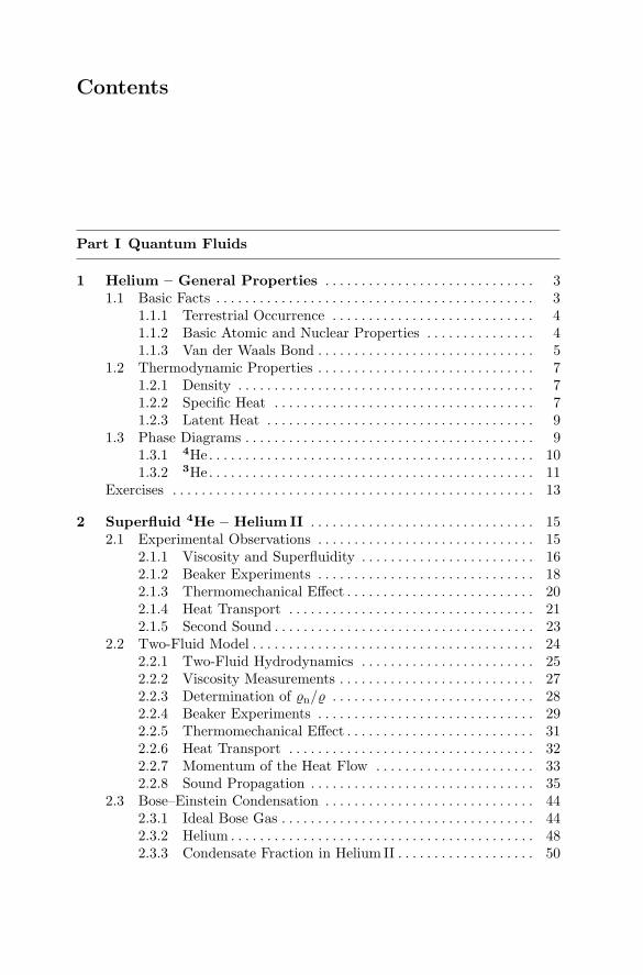
Contents
Part I Quantum Fluids
1 Helium – General Properties . . . . . . . . . . . . . . . . . . . . . . . . . . . . . 31.1 Basic Facts . . . . . . . . . . . . . . . . . . . . . . . . . . . . . . . . . . . . . . . . . . . . 3
1.1.1 Terrestrial Occurrence . . . . . . . . . . . . . . . . . . . . . . . . . . . . 41.1.2 Basic Atomic and Nuclear Properties . . . . . . . . . . . . . . . 41.1.3 Van der Waals Bond . . . . . . . . . . . . . . . . . . . . . . . . . . . . . . 5
1.2 Thermodynamic Properties . . . . . . . . . . . . . . . . . . . . . . . . . . . . . . 71.2.1 Density . . . . . . . . . . . . . . . . . . . . . . . . . . . . . . . . . . . . . . . . . 71.2.2 Specific Heat . . . . . . . . . . . . . . . . . . . . . . . . . . . . . . . . . . . . 71.2.3 Latent Heat . . . . . . . . . . . . . . . . . . . . . . . . . . . . . . . . . . . . . 9
1.3 Phase Diagrams . . . . . . . . . . . . . . . . . . . . . . . . . . . . . . . . . . . . . . . . 91.3.1 4He. . . . . . . . . . . . . . . . . . . . . . . . . . . . . . . . . . . . . . . . . . . . . 101.3.2 3He. . . . . . . . . . . . . . . . . . . . . . . . . . . . . . . . . . . . . . . . . . . . . 11
Exercises . . . . . . . . . . . . . . . . . . . . . . . . . . . . . . . . . . . . . . . . . . . . . . . . . . 13
2 Superfluid 4He – Helium II . . . . . . . . . . . . . . . . . . . . . . . . . . . . . . . 152.1 Experimental Observations . . . . . . . . . . . . . . . . . . . . . . . . . . . . . . 15
2.1.1 Viscosity and Superfluidity . . . . . . . . . . . . . . . . . . . . . . . . 162.1.2 Beaker Experiments . . . . . . . . . . . . . . . . . . . . . . . . . . . . . . 182.1.3 Thermomechanical Effect . . . . . . . . . . . . . . . . . . . . . . . . . . 202.1.4 Heat Transport . . . . . . . . . . . . . . . . . . . . . . . . . . . . . . . . . . 212.1.5 Second Sound . . . . . . . . . . . . . . . . . . . . . . . . . . . . . . . . . . . . 23
2.2 Two-Fluid Model . . . . . . . . . . . . . . . . . . . . . . . . . . . . . . . . . . . . . . . 242.2.1 Two-Fluid Hydrodynamics . . . . . . . . . . . . . . . . . . . . . . . . 252.2.2 Viscosity Measurements . . . . . . . . . . . . . . . . . . . . . . . . . . . 272.2.3 Determination of ϱn/ϱ . . . . . . . . . . . . . . . . . . . . . . . . . . . . 282.2.4 Beaker Experiments . . . . . . . . . . . . . . . . . . . . . . . . . . . . . . 292.2.5 Thermomechanical Effect . . . . . . . . . . . . . . . . . . . . . . . . . . 312.2.6 Heat Transport . . . . . . . . . . . . . . . . . . . . . . . . . . . . . . . . . . 322.2.7 Momentum of the Heat Flow . . . . . . . . . . . . . . . . . . . . . . 332.2.8 Sound Propagation . . . . . . . . . . . . . . . . . . . . . . . . . . . . . . . 35
2.3 Bose–Einstein Condensation . . . . . . . . . . . . . . . . . . . . . . . . . . . . . 442.3.1 Ideal Bose Gas . . . . . . . . . . . . . . . . . . . . . . . . . . . . . . . . . . . 442.3.2 Helium . . . . . . . . . . . . . . . . . . . . . . . . . . . . . . . . . . . . . . . . . . 482.3.3 Condensate Fraction in Helium II . . . . . . . . . . . . . . . . . . . 50
VIII Contents
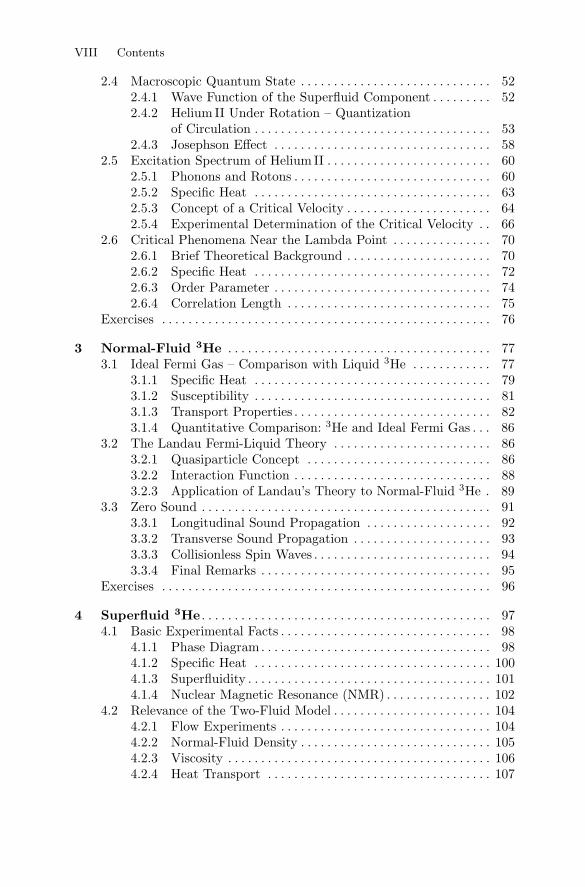
2.4 Macroscopic Quantum State . . . . . . . . . . . . . . . . . . . . . . . . . . . . . 522.4.1 Wave Function of the Superfluid Component . . . . . . . . . 522.4.2 Helium II Under Rotation – Quantization
of Circulation . . . . . . . . . . . . . . . . . . . . . . . . . . . . . . . . . . . . 532.4.3 Josephson Effect . . . . . . . . . . . . . . . . . . . . . . . . . . . . . . . . . 58
2.5 Excitation Spectrum of Helium II . . . . . . . . . . . . . . . . . . . . . . . . . 602.5.1 Phonons and Rotons . . . . . . . . . . . . . . . . . . . . . . . . . . . . . . 602.5.2 Specific Heat . . . . . . . . . . . . . . . . . . . . . . . . . . . . . . . . . . . . 632.5.3 Concept of a Critical Velocity . . . . . . . . . . . . . . . . . . . . . . 642.5.4 Experimental Determination of the Critical Velocity . . 66
2.6 Critical Phenomena Near the Lambda Point . . . . . . . . . . . . . . . 702.6.1 Brief Theoretical Background . . . . . . . . . . . . . . . . . . . . . . 702.6.2 Specific Heat . . . . . . . . . . . . . . . . . . . . . . . . . . . . . . . . . . . . 722.6.3 Order Parameter . . . . . . . . . . . . . . . . . . . . . . . . . . . . . . . . . 742.6.4 Correlation Length . . . . . . . . . . . . . . . . . . . . . . . . . . . . . . . 75
Exercises . . . . . . . . . . . . . . . . . . . . . . . . . . . . . . . . . . . . . . . . . . . . . . . . . . 76
3 Normal-Fluid 3He . . . . . . . . . . . . . . . . . . . . . . . . . . . . . . . . . . . . . . . . 773.1 Ideal Fermi Gas – Comparison with Liquid 3He . . . . . . . . . . . . 77
3.1.1 Specific Heat . . . . . . . . . . . . . . . . . . . . . . . . . . . . . . . . . . . . 793.1.2 Susceptibility . . . . . . . . . . . . . . . . . . . . . . . . . . . . . . . . . . . . 813.1.3 Transport Properties . . . . . . . . . . . . . . . . . . . . . . . . . . . . . . 823.1.4 Quantitative Comparison: 3He and Ideal Fermi Gas . . . 86
3.2 The Landau Fermi-Liquid Theory . . . . . . . . . . . . . . . . . . . . . . . . 863.2.1 Quasiparticle Concept . . . . . . . . . . . . . . . . . . . . . . . . . . . . 863.2.2 Interaction Function . . . . . . . . . . . . . . . . . . . . . . . . . . . . . . 883.2.3 Application of Landau’s Theory to Normal-Fluid 3He . 89
3.3 Zero Sound . . . . . . . . . . . . . . . . . . . . . . . . . . . . . . . . . . . . . . . . . . . . 913.3.1 Longitudinal Sound Propagation . . . . . . . . . . . . . . . . . . . 923.3.2 Transverse Sound Propagation . . . . . . . . . . . . . . . . . . . . . 933.3.3 Collisionless Spin Waves . . . . . . . . . . . . . . . . . . . . . . . . . . . 943.3.4 Final Remarks . . . . . . . . . . . . . . . . . . . . . . . . . . . . . . . . . . . 95
Exercises . . . . . . . . . . . . . . . . . . . . . . . . . . . . . . . . . . . . . . . . . . . . . . . . . . 96
4 Superfluid 3He . . . . . . . . . . . . . . . . . . . . . . . . . . . . . . . . . . . . . . . . . . . . 974.1 Basic Experimental Facts . . . . . . . . . . . . . . . . . . . . . . . . . . . . . . . . 98
4.1.1 Phase Diagram. . . . . . . . . . . . . . . . . . . . . . . . . . . . . . . . . . . 984.1.2 Specific Heat . . . . . . . . . . . . . . . . . . . . . . . . . . . . . . . . . . . . 1004.1.3 Superfluidity . . . . . . . . . . . . . . . . . . . . . . . . . . . . . . . . . . . . . 1014.1.4 Nuclear Magnetic Resonance (NMR) . . . . . . . . . . . . . . . . 102
4.2 Relevance of the Two-Fluid Model . . . . . . . . . . . . . . . . . . . . . . . . 1044.2.1 Flow Experiments . . . . . . . . . . . . . . . . . . . . . . . . . . . . . . . . 1044.2.2 Normal-Fluid Density . . . . . . . . . . . . . . . . . . . . . . . . . . . . . 1054.2.3 Viscosity . . . . . . . . . . . . . . . . . . . . . . . . . . . . . . . . . . . . . . . . 1064.2.4 Heat Transport . . . . . . . . . . . . . . . . . . . . . . . . . . . . . . . . . . 107

Contents IX
4.3 Quantum States of Pairs of Coupled Quasiparticles . . . . . . . . . 1074.3.1 Spin-Triplet Pairing . . . . . . . . . . . . . . . . . . . . . . . . . . . . . . 1084.3.2 Broken Symmetry in Superfluid 3He . . . . . . . . . . . . . . . . 1104.3.3 Energy Gap and Superfluidity . . . . . . . . . . . . . . . . . . . . . . 112
4.4 Order-Parameter Orientation – Textures . . . . . . . . . . . . . . . . . . 1144.4.1 Intrinsic Alignment . . . . . . . . . . . . . . . . . . . . . . . . . . . . . . . 1154.4.2 Textures in 3He-A . . . . . . . . . . . . . . . . . . . . . . . . . . . . . . . . 1164.4.3 Surface-induced Texture – 3He-A in a Slab . . . . . . . . . . 1184.4.4 Textures in 3He-B . . . . . . . . . . . . . . . . . . . . . . . . . . . . . . . . 119
4.5 Spin Dynamics – NMR Experiments . . . . . . . . . . . . . . . . . . . . . . 1204.5.1 Leggett Equations . . . . . . . . . . . . . . . . . . . . . . . . . . . . . . . . 1204.5.2 Transverse Resonance – Frequency Shift . . . . . . . . . . . . . 1214.5.3 Longitudinal Resonance . . . . . . . . . . . . . . . . . . . . . . . . . . . 122
4.6 Macroscopic Quantum Effects . . . . . . . . . . . . . . . . . . . . . . . . . . . . 1244.6.1 Superflow . . . . . . . . . . . . . . . . . . . . . . . . . . . . . . . . . . . . . . . 1244.6.2 Quantization of Circulation . . . . . . . . . . . . . . . . . . . . . . . . 1254.6.3 Quantized Vortices . . . . . . . . . . . . . . . . . . . . . . . . . . . . . . . 1274.6.4 Macroscopic Quantum Interference –
Josephson Effect . . . . . . . . . . . . . . . . . . . . . . . . . . . . . . . . . 1314.7 Normal-Fluid Density – Quasiparticle Scattering . . . . . . . . . . . 134
4.7.1 Normal-Fluid Density . . . . . . . . . . . . . . . . . . . . . . . . . . . . . 1344.7.2 Specific Heat . . . . . . . . . . . . . . . . . . . . . . . . . . . . . . . . . . . . 1354.7.3 Quasiparticle Scattering . . . . . . . . . . . . . . . . . . . . . . . . . . . 136
4.8 Collective Excitations – Sound Propagation . . . . . . . . . . . . . . . . 1374.8.1 Sound Propagation . . . . . . . . . . . . . . . . . . . . . . . . . . . . . . . 1384.8.2 Collective Order-Parameter Modes . . . . . . . . . . . . . . . . . 142
Exercises . . . . . . . . . . . . . . . . . . . . . . . . . . . . . . . . . . . . . . . . . . . . . . . . . . 146
5 Mixtures of 3He and 4He . . . . . . . . . . . . . . . . . . . . . . . . . . . . . . . . . 1475.1 Specific Heat, Phase Diagram and Solubility . . . . . . . . . . . . . . . 148
5.1.1 Phase Diagram. . . . . . . . . . . . . . . . . . . . . . . . . . . . . . . . . . . 1495.1.2 Specific Heat of Dilute Solutions of 3He in Helium II . . 1505.1.3 Finite Solubility of 3He in Liquid 4He at T = 0 . . . . . . . 151
5.2 Normal-Fluid Component . . . . . . . . . . . . . . . . . . . . . . . . . . . . . . . 1535.2.1 Andronikashvili Experiment . . . . . . . . . . . . . . . . . . . . . . . 1535.2.2 Osmotic Pressure . . . . . . . . . . . . . . . . . . . . . . . . . . . . . . . . . 154
5.3 Sound Propagation . . . . . . . . . . . . . . . . . . . . . . . . . . . . . . . . . . . . . 1555.3.1 First Sound . . . . . . . . . . . . . . . . . . . . . . . . . . . . . . . . . . . . . . 1565.3.2 Second Sound . . . . . . . . . . . . . . . . . . . . . . . . . . . . . . . . . . . . 157
5.4 Transport Properties . . . . . . . . . . . . . . . . . . . . . . . . . . . . . . . . . . . . 1585.4.1 Heat Transport . . . . . . . . . . . . . . . . . . . . . . . . . . . . . . . . . . 1585.4.2 Viscosity . . . . . . . . . . . . . . . . . . . . . . . . . . . . . . . . . . . . . . . . 1595.4.3 Self-Diffusion Coefficient . . . . . . . . . . . . . . . . . . . . . . . . . . 160
5.5 Search for a Superfluid Phase of 3He in Mixtures . . . . . . . . . . . 161Exercises . . . . . . . . . . . . . . . . . . . . . . . . . . . . . . . . . . . . . . . . . . . . . . . . . . 163
X Contents
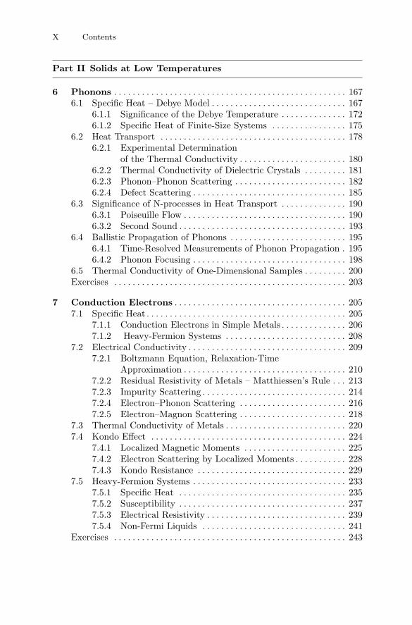
Part II Solids at Low Temperatures
6 Phonons . . . . . . . . . . . . . . . . . . . . . . . . . . . . . . . . . . . . . . . . . . . . . . . . . . 1676.1 Specific Heat – Debye Model . . . . . . . . . . . . . . . . . . . . . . . . . . . . . 167
6.1.1 Significance of the Debye Temperature . . . . . . . . . . . . . . 1726.1.2 Specific Heat of Finite-Size Systems . . . . . . . . . . . . . . . . 175
6.2 Heat Transport . . . . . . . . . . . . . . . . . . . . . . . . . . . . . . . . . . . . . . . . 1786.2.1 Experimental Determination
of the Thermal Conductivity . . . . . . . . . . . . . . . . . . . . . . . 1806.2.2 Thermal Conductivity of Dielectric Crystals . . . . . . . . . 1816.2.3 Phonon–Phonon Scattering . . . . . . . . . . . . . . . . . . . . . . . . 1826.2.4 Defect Scattering . . . . . . . . . . . . . . . . . . . . . . . . . . . . . . . . . 185
6.3 Significance of N-processes in Heat Transport . . . . . . . . . . . . . . 1906.3.1 Poiseuille Flow . . . . . . . . . . . . . . . . . . . . . . . . . . . . . . . . . . . 1906.3.2 Second Sound . . . . . . . . . . . . . . . . . . . . . . . . . . . . . . . . . . . . 193
6.4 Ballistic Propagation of Phonons . . . . . . . . . . . . . . . . . . . . . . . . . 1956.4.1 Time-Resolved Measurements of Phonon Propagation . 1956.4.2 Phonon Focusing . . . . . . . . . . . . . . . . . . . . . . . . . . . . . . . . . 198
6.5 Thermal Conductivity of One-Dimensional Samples . . . . . . . . . 200Exercises . . . . . . . . . . . . . . . . . . . . . . . . . . . . . . . . . . . . . . . . . . . . . . . . . . 203
7 Conduction Electrons . . . . . . . . . . . . . . . . . . . . . . . . . . . . . . . . . . . . . 2057.1 Specific Heat . . . . . . . . . . . . . . . . . . . . . . . . . . . . . . . . . . . . . . . . . . . 205
7.1.1 Conduction Electrons in Simple Metals . . . . . . . . . . . . . . 2067.1.2 Heavy-Fermion Systems . . . . . . . . . . . . . . . . . . . . . . . . . . 208
7.2 Electrical Conductivity . . . . . . . . . . . . . . . . . . . . . . . . . . . . . . . . . . 2097.2.1 Boltzmann Equation, Relaxation-Time
Approximation . . . . . . . . . . . . . . . . . . . . . . . . . . . . . . . . . . . 2107.2.2 Residual Resistivity of Metals – Matthiessen’s Rule . . . 2137.2.3 Impurity Scattering . . . . . . . . . . . . . . . . . . . . . . . . . . . . . . . 2147.2.4 Electron–Phonon Scattering . . . . . . . . . . . . . . . . . . . . . . . 2167.2.5 Electron–Magnon Scattering . . . . . . . . . . . . . . . . . . . . . . . 218
7.3 Thermal Conductivity of Metals . . . . . . . . . . . . . . . . . . . . . . . . . . 2207.4 Kondo Effect . . . . . . . . . . . . . . . . . . . . . . . . . . . . . . . . . . . . . . . . . . 224
7.4.1 Localized Magnetic Moments . . . . . . . . . . . . . . . . . . . . . . 2257.4.2 Electron Scattering by Localized Moments . . . . . . . . . . . 2287.4.3 Kondo Resistance . . . . . . . . . . . . . . . . . . . . . . . . . . . . . . . . 229
7.5 Heavy-Fermion Systems . . . . . . . . . . . . . . . . . . . . . . . . . . . . . . . . . 2337.5.1 Specific Heat . . . . . . . . . . . . . . . . . . . . . . . . . . . . . . . . . . . . 2357.5.2 Susceptibility . . . . . . . . . . . . . . . . . . . . . . . . . . . . . . . . . . . . 2377.5.3 Electrical Resistivity . . . . . . . . . . . . . . . . . . . . . . . . . . . . . . 2397.5.4 Non-Fermi Liquids . . . . . . . . . . . . . . . . . . . . . . . . . . . . . . . 241
Exercises . . . . . . . . . . . . . . . . . . . . . . . . . . . . . . . . . . . . . . . . . . . . . . . . . . 243

Contents XI
8 Magnetic Moments – Spins . . . . . . . . . . . . . . . . . . . . . . . . . . . . . . . 2458.1 Paramagnetic Systems – Isolated Spins . . . . . . . . . . . . . . . . . . . . 245
8.1.1 Magnetic Moments . . . . . . . . . . . . . . . . . . . . . . . . . . . . . . . 2468.1.2 Susceptibility . . . . . . . . . . . . . . . . . . . . . . . . . . . . . . . . . . . . 2478.1.3 Specific Heat . . . . . . . . . . . . . . . . . . . . . . . . . . . . . . . . . . . . 249
8.2 Spin Waves – Magnons . . . . . . . . . . . . . . . . . . . . . . . . . . . . . . . . . . 2578.2.1 Ferromagnets . . . . . . . . . . . . . . . . . . . . . . . . . . . . . . . . . . . . 2578.2.2 Antiferromagnets . . . . . . . . . . . . . . . . . . . . . . . . . . . . . . . . . 262
8.3 Spin Glasses . . . . . . . . . . . . . . . . . . . . . . . . . . . . . . . . . . . . . . . . . . . 2648.3.1 Structural Properties . . . . . . . . . . . . . . . . . . . . . . . . . . . . . 2658.3.2 Dynamic Behavior . . . . . . . . . . . . . . . . . . . . . . . . . . . . . . . . 2678.3.3 Ageing, Rejuvenation and Memory Effects . . . . . . . . . . . 268
8.4 Nuclear Magnetic Ordering . . . . . . . . . . . . . . . . . . . . . . . . . . . . . . 2718.4.1 Strong Nucleus–Electron Coupling . . . . . . . . . . . . . . . . . . 2728.4.2 Weak Nucleus–Electron Coupling . . . . . . . . . . . . . . . . . . . 275
8.5 Negative Spin Temperatures . . . . . . . . . . . . . . . . . . . . . . . . . . . . . 2778.5.1 Thermodynamics at Negative Temperatures . . . . . . . . . 2788.5.2 Nuclear Ordering . . . . . . . . . . . . . . . . . . . . . . . . . . . . . . . . . 2808.5.3 Stimulated Emission . . . . . . . . . . . . . . . . . . . . . . . . . . . . . . 281
Exercises . . . . . . . . . . . . . . . . . . . . . . . . . . . . . . . . . . . . . . . . . . . . . . . . . . 282
9 Tunneling Systems . . . . . . . . . . . . . . . . . . . . . . . . . . . . . . . . . . . . . . . . 2839.1 Two-Level Tunneling Systems . . . . . . . . . . . . . . . . . . . . . . . . . . . . 283
9.1.1 Double-Well Potentials . . . . . . . . . . . . . . . . . . . . . . . . . . . . 2849.1.2 Coupling to Electric and Elastic Fields . . . . . . . . . . . . . . 2859.1.3 Relaxation . . . . . . . . . . . . . . . . . . . . . . . . . . . . . . . . . . . . . . 2869.1.4 Relaxation Times . . . . . . . . . . . . . . . . . . . . . . . . . . . . . . . . 2909.1.5 Resonant Interaction . . . . . . . . . . . . . . . . . . . . . . . . . . . . . . 292
9.2 Isolated Tunneling Systems in Crystals . . . . . . . . . . . . . . . . . . . . 2949.2.1 Level Schemes . . . . . . . . . . . . . . . . . . . . . . . . . . . . . . . . . . . 2949.2.2 Specific Heat . . . . . . . . . . . . . . . . . . . . . . . . . . . . . . . . . . . . 2989.2.3 Thermal Conductivity . . . . . . . . . . . . . . . . . . . . . . . . . . . . 3009.2.4 Level Crossing . . . . . . . . . . . . . . . . . . . . . . . . . . . . . . . . . . . 3029.2.5 Dielectric Susceptibility . . . . . . . . . . . . . . . . . . . . . . . . . . . 3039.2.6 Sound Velocity . . . . . . . . . . . . . . . . . . . . . . . . . . . . . . . . . . . 306
9.3 Interacting Tunneling Systems in Crystals . . . . . . . . . . . . . . . . . 3089.3.1 Dielectric Properties . . . . . . . . . . . . . . . . . . . . . . . . . . . . . . 3089.3.2 Theoretical Description . . . . . . . . . . . . . . . . . . . . . . . . . . . 3099.3.3 Dielectric Susceptibility . . . . . . . . . . . . . . . . . . . . . . . . . . . 311
9.4 Asymmetric Tunneling Systems in Crystals . . . . . . . . . . . . . . . . 3149.4.1 Nb:O,H and Nb:O,D . . . . . . . . . . . . . . . . . . . . . . . . . . . . . . 3149.4.2 CN− Ions in KBr:KCl . . . . . . . . . . . . . . . . . . . . . . . . . . . . . 316

XII Contents
9.5 Amorphous Dielectrics . . . . . . . . . . . . . . . . . . . . . . . . . . . . . . . . . . 3179.5.1 Specific Heat . . . . . . . . . . . . . . . . . . . . . . . . . . . . . . . . . . . . 3189.5.2 Thermal Conductivity . . . . . . . . . . . . . . . . . . . . . . . . . . . . 3239.5.3 Relaxation Absorption . . . . . . . . . . . . . . . . . . . . . . . . . . . . 3259.5.4 Resonant Absorption . . . . . . . . . . . . . . . . . . . . . . . . . . . . . 3279.5.5 Sound Velocity and Dielectric Constant . . . . . . . . . . . . . 330
9.6 Metallic Glasses . . . . . . . . . . . . . . . . . . . . . . . . . . . . . . . . . . . . . . . . 3339.7 Echo Experiments . . . . . . . . . . . . . . . . . . . . . . . . . . . . . . . . . . . . . . 334Exercises . . . . . . . . . . . . . . . . . . . . . . . . . . . . . . . . . . . . . . . . . . . . . . . . . . 340
10 Superconductivity . . . . . . . . . . . . . . . . . . . . . . . . . . . . . . . . . . . . . . . . 34310.1 Experimental Observations . . . . . . . . . . . . . . . . . . . . . . . . . . . . . . 343
10.1.1 Transition Temperature . . . . . . . . . . . . . . . . . . . . . . . . . . . 34510.1.2 Meissner–Ochsenfeld Effect . . . . . . . . . . . . . . . . . . . . . . . . 34710.1.3 Type I Superconductor . . . . . . . . . . . . . . . . . . . . . . . . . . . . 35010.1.4 Type II Superconductors . . . . . . . . . . . . . . . . . . . . . . . . . . 354
10.2 Phenomenological Description . . . . . . . . . . . . . . . . . . . . . . . . . . . . 35710.2.1 Thermodynamics of Superconductors . . . . . . . . . . . . . . . 35810.2.2 London Equations . . . . . . . . . . . . . . . . . . . . . . . . . . . . . . . . 36210.2.3 Pippard’s Equation . . . . . . . . . . . . . . . . . . . . . . . . . . . . . . . 36610.2.4 Ginzburg–Landau Theory . . . . . . . . . . . . . . . . . . . . . . . . . 367
10.3 Microscopic Theory of Superconductivity . . . . . . . . . . . . . . . . . . 37610.3.1 Cooper Pairs . . . . . . . . . . . . . . . . . . . . . . . . . . . . . . . . . . . . 37610.3.2 BCS Ground State . . . . . . . . . . . . . . . . . . . . . . . . . . . . . . . 38110.3.3 Excitation of the BCS Ground State . . . . . . . . . . . . . . . . 38510.3.4 BCS State at Finite Temperatures . . . . . . . . . . . . . . . . . . 38710.3.5 Measurement of the Energy Gap . . . . . . . . . . . . . . . . . . . 39010.3.6 Tunneling Experiments . . . . . . . . . . . . . . . . . . . . . . . . . . . . 39410.3.7 Critical Current and Energy Gap . . . . . . . . . . . . . . . . . . . 399
10.4 Flux Quantization – Josephson Effect . . . . . . . . . . . . . . . . . . . . . 40010.4.1 Flux Quantization . . . . . . . . . . . . . . . . . . . . . . . . . . . . . . . . 40110.4.2 Pair Tunneling – Josephson Effect . . . . . . . . . . . . . . . . . . 40410.4.3 Quantum Interference . . . . . . . . . . . . . . . . . . . . . . . . . . . . . 40810.4.4 Superconducting Magnetometer – SQUID . . . . . . . . . . . 410
10.5 Superconductors with Unusual Properties . . . . . . . . . . . . . . . . . 41310.5.1 Organic Superconductors . . . . . . . . . . . . . . . . . . . . . . . . . . 41510.5.2 Magnetism and Superconductivity . . . . . . . . . . . . . . . . . . 41810.5.3 Heavy-Fermion Superconductors . . . . . . . . . . . . . . . . . . . 42810.5.4 High-Tc Superconductors . . . . . . . . . . . . . . . . . . . . . . . . . . 432
Exercises . . . . . . . . . . . . . . . . . . . . . . . . . . . . . . . . . . . . . . . . . . . . . . . . . . 446

Contents XIII
Part III Principles of Refrigeration and Thermometry
11 Cooling Techniques . . . . . . . . . . . . . . . . . . . . . . . . . . . . . . . . . . . . . . . 44911.1 Liquefaction of Gases . . . . . . . . . . . . . . . . . . . . . . . . . . . . . . . . . . . 450
11.1.1 Expansion Engines . . . . . . . . . . . . . . . . . . . . . . . . . . . . . . . 45111.1.2 Joule–Thomson Expansion . . . . . . . . . . . . . . . . . . . . . . . . 457
11.2 Closed-Cycle Refrigerators . . . . . . . . . . . . . . . . . . . . . . . . . . . . . . . 46011.2.1 Gifford–McMahon Coolers . . . . . . . . . . . . . . . . . . . . . . . . . 46011.2.2 Pulse-Tube Coolers . . . . . . . . . . . . . . . . . . . . . . . . . . . . . . . 462
11.3 Simple Helium-Bath Cryostats . . . . . . . . . . . . . . . . . . . . . . . . . . . 46411.3.1 Bath Cryostats . . . . . . . . . . . . . . . . . . . . . . . . . . . . . . . . . . . 46411.3.2 Evaporation Cryostats . . . . . . . . . . . . . . . . . . . . . . . . . . . . 467
11.4 Dilution Refrigerators . . . . . . . . . . . . . . . . . . . . . . . . . . . . . . . . . . . 47111.4.1 Principle of Operation . . . . . . . . . . . . . . . . . . . . . . . . . . . . 47111.4.2 Principles of a Dilution Refrigerator . . . . . . . . . . . . . . . . 47211.4.3 Problem of the Thermal Boundary Resistance . . . . . . . . 47411.4.4 Cooling Power . . . . . . . . . . . . . . . . . . . . . . . . . . . . . . . . . . . 478
11.5 Pomeranchuk Cooling . . . . . . . . . . . . . . . . . . . . . . . . . . . . . . . . . . . 48011.5.1 Cooling by Solidification of 3He . . . . . . . . . . . . . . . . . . . . 48111.5.2 Technical Realization . . . . . . . . . . . . . . . . . . . . . . . . . . . . . 48111.5.3 Cooling Power . . . . . . . . . . . . . . . . . . . . . . . . . . . . . . . . . . . 482
11.6 Adiabatic Demagnetization . . . . . . . . . . . . . . . . . . . . . . . . . . . . . . 48311.6.1 Cooling Mechanism . . . . . . . . . . . . . . . . . . . . . . . . . . . . . . . 48411.6.2 Cooling Capacity and Minimum Temperature . . . . . . . . 48611.6.3 Electron Spins – Paramagnetic Salts . . . . . . . . . . . . . . . . 487
11.7 Nuclear Spin Demagnetization . . . . . . . . . . . . . . . . . . . . . . . . . . . 48911.7.1 Coupling of Nuclear Spins and Conduction Electrons . . 48911.7.2 Influence of Heat Leaks . . . . . . . . . . . . . . . . . . . . . . . . . . . 49111.7.3 Sources of Heat Leaks . . . . . . . . . . . . . . . . . . . . . . . . . . . . . 49111.7.4 Technical Features . . . . . . . . . . . . . . . . . . . . . . . . . . . . . . . . 497
Exercises . . . . . . . . . . . . . . . . . . . . . . . . . . . . . . . . . . . . . . . . . . . . . . . . . . 504
12 Thermometry . . . . . . . . . . . . . . . . . . . . . . . . . . . . . . . . . . . . . . . . . . . . . 50512.1 Primary Thermometers . . . . . . . . . . . . . . . . . . . . . . . . . . . . . . . . . 506
12.1.1 Gas Thermometers . . . . . . . . . . . . . . . . . . . . . . . . . . . . . . . 50612.1.2 Vapor-Pressure Thermometers . . . . . . . . . . . . . . . . . . . . . 50612.1.3 3He Melting-Curve Thermometer . . . . . . . . . . . . . . . . . . . 50812.1.4 Noise Thermometers . . . . . . . . . . . . . . . . . . . . . . . . . . . . . . 51012.1.5 Superconducting Fixed-Point Thermometers . . . . . . . . . 51412.1.6 Nuclear-Orientation Thermometers . . . . . . . . . . . . . . . . . 51612.1.7 Mossbauer-Effect Thermometers . . . . . . . . . . . . . . . . . . . 51912.1.8 Coulomb-Blockade Thermometers . . . . . . . . . . . . . . . . . . 52012.1.9 Osmotic-Pressure Thermometers . . . . . . . . . . . . . . . . . . . 522
12.2 Secondary Thermometers . . . . . . . . . . . . . . . . . . . . . . . . . . . . . . . . 522

XIV Contents
12.2.1 Resistance Thermometers . . . . . . . . . . . . . . . . . . . . . . . . . 52212.2.2 Thermoelectric Elements . . . . . . . . . . . . . . . . . . . . . . . . . . 53112.2.3 Capacitive Thermometers . . . . . . . . . . . . . . . . . . . . . . . . . 53212.2.4 Magnetic Thermometers . . . . . . . . . . . . . . . . . . . . . . . . . . 53312.2.5 Nuclear Spin Resonance Thermometers . . . . . . . . . . . . . 537
Exercises . . . . . . . . . . . . . . . . . . . . . . . . . . . . . . . . . . . . . . . . . . . . . . . . . . 541
References . . . . . . . . . . . . . . . . . . . . . . . . . . . . . . . . . . . . . . . . . . . . . . . . . . . . 543
Index . . . . . . . . . . . . . . . . . . . . . . . . . . . . . . . . . . . . . . . . . . . . . . . . . . . . . . . . . 563

Part I
Quantum Fluids

1 Helium – General Properties
Evidence for the existence of the rare noble gas helium was first obtainedby the French astronomer Janssen in the visible spectrum of solar protuber-ances during a total eclipse in 1868 in India [1]. Using a spectrometer, henoticed a hitherto unknown yellow line. Shortly afterwards, his observationwas confirmed by Lockyer , an English astronomer [2]. He related the newspectral line to a chemical element that had not been seen on Earth beforeand suggested the name helium for it after helios, the Greek name for sun.On Earth, the helium was discovered in 1895 by Ramsay [3] and indepen-dently by Cleve and Langlet [4] in celveite, a rocksand mineral that containsuranium and thorium. Later in the same year, helium was also found in gasevolving from a spring in Bad Wildbad in the Black Forest in Germany byKayser [5].
Only a few years after the discovery of helium on Earth, a race tookplace between several competing low-temperature laboratories with the aimof being the first to liquefy this last of the so-called permanent gases. Onemajor difficulty was to obtain sufficient quantities of helium gas. With thehelp of his brother, who was the director of the Department of Foreign TradeRelations in Amsterdam, Kamerlingh Onnes, the head of the laboratory inLeiden, managed to get a ship load of monazite sand from North Carolinafrom which he and his coworkers extracted 360 liters of helium gas. He reachedthe goal of liquefaction of helium on 10 July 1908 [6]. With the achievementof this milestone he established modern low-temperature physics. For manyyears, the laboratory in Leiden was the leader in this new field.
1.1 Basic Facts
At room temperature, helium is a light inert gas. It is odorless, colorless,and tasteless, and, after hydrogen, the second most abundant element in theuniverse. Despite its very simple structure, helium exhibits numerous exoticphenomena in condensed form whose theoretical descriptions are rather com-plex in many cases. We will take a look at some of the unusual characteristicsof quantum fluids and quantum solids in the following chapters. To begin,however, let us introduce some general properties of helium in the remainingpart of this chapter.

4 1 Helium – General Properties
1.1.1 Terrestrial Occurrence
Helium exists in two stable isotopes. 4He makes up about 5.2 ppm of theEarth’s atmosphere. This trace amount of helium is not gravitationally boundto the Earth and is constantly lost into space. The Earth’s atmospheric he-lium is replaced by the decay of radioactive elements in the crust of theEarth. Whereas in the early days of helium research, 4He gas was mainlyobtained from minerals, today it is recovered exclusively from natural-gasdeposits. The largest sources of helium-rich natural gas are located in theUnited States. The chemical composition and the helium content of naturalgas differs widely, depending on the geological strata. In some natural-gaswells a helium content up to 7% has been found.
The lighter isotope 3He was discovered and identified in 1933 by Oliphant,Kinsey and Rutherford [7]. At first, however, it was believed that 3He shouldnot be stable. This misconception was disproved in 1939 by Alvarez andCornog in cyclotron accelerator experiments [8]. To obtain 3He in quanti-ties for use in low-temperature physics experiments, it has to be producedartificially via nuclear reactions, because the concentration of 3He in heliumfrom natural-gas sources is only 0.14 ppm. Therefore, the production of 3Herelies on waste from nuclear reactors or the waste from various constituentsof hydrogen bombs. The nuclear reaction is
6Li + n −→ 3H + 4He (1.1)|−→ 3He + e− + νe .
In the first step of this reaction, tritium is produced that has a half-lifeof 12.5 years. It undergoes beta decay with 3He as a product. Significantamounts of 3He were not available before the end of the 1950s. Nevertheless,Sydoriak, Grilly and Hammel managed to liquefy 3He as early as 1949 andinvestigated its properties [9].
1.1.2 Basic Atomic and Nuclear Properties
The electronic structure of helium is the simplest many-body system of allatoms. With two electrons completely filling the K shell (1s2 ) it has a sphericalshape and thus no permanent electric dipole moment. Helium has the smallestknown atomic polarizability of α = 0.1232 cm3 mol−1 and only a very weakdiamagnetic susceptibility χd = −1.9 ×10⁻⁶ cm3 mol−1. With an atomicradius of only 31 pm it is the smallest atom. It has the highest ionizationenergy of about 24.6 eV.
The liquid of both isotopes is colorless and since their index of refraction isvery close to unity, they are very difficult to see. Because of their nuclear spinI = 1/2, 3He atoms are fermions and obey Fermi–Dirac statistics, whereas4He atoms are bosons with nuclear spin I = 0. Besides the two stable isotopes3He and 4He, there exist two unstable helium isotopes with relatively longhalf-lives: 6He (T1/ 2 = 0.82 s), and 8He (T1/ 2 = 0.12 s).

1.1 Basic Facts 5
1.1.3 Van der Waals Bond
Van der Waals forces act between all atoms. They are based upon the elec-trical dipole–dipole interaction. At first glance the appearance of this typeof force between helium atoms is surprising, because, as mentioned above,they have perfect spherical symmetry and thus no permanent electrical di-pole moment. However, one has to take into account that there are alwayszero-point fluctuations present in the charge distribution, which result in fluc-tuating dipole moments. The associated electrical fields induce fluctuating di-pole moments at neighboring atoms as well and thus lead to a force betweenthe atoms. This force can be described using the Van der Waals potentialφ(r) ∝ 1/r6 , where r denotes the interatomic distance. In the framework ofa quantum-mechanical treatment of the Van der Waals force one can showthat this type of interaction always leads to an energy reduction and thus toan attractive force. The strength of this force is given by the polarizability ofthe interacting atoms. Since the polarizability is small in the case of heliumatoms, the binding force is very weak.
By adding a repulsive potential of the form φ(r) ∝ 1/r12 one obtains thewell-known Lennard–Jones potential [10]
φ(r) = 4ε!"σ
r
#12−
"σ
r
#6$
, (1.2)
with the characteristic parameters ε and σ. For both helium isotopes wehave ε/kB = 10.2K and σ = 2.56 A. The potential energy is obtained byintegrating (1.2)
Epot =12
∞%
0
φ(r) 4πr2n(r) dr , (1.3)
taking into account the radial density function n(r). The difference in thepotential energy of liquid and solid helium originates from the difference inn(r) of the two phases.
In addition to the very weak binding forces between helium atoms, thereis a reduction of the binding by the zero-point motion. Although a detailedcalculation of the zero-point energy of helium in the liquid phase is rathercomplex, we can estimate the size of this effect in a simple model in whichwe assign each atom a certain ‘cage’ volume V . The ground-state energy(zero-point energy) of a particle with mass m in such a cage is given by
E0 =3!2π2
2mV 2 / 3. (1.4)
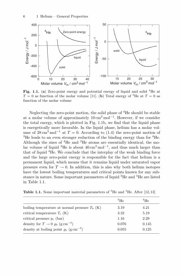
From this result, we can directly see that the zero-point energy for atomswith a small mass like helium is large and that it increases with decreasingmolar volume Vm. In Fig. 1.1a the zero-point energy of 4He is plotted as afunction of the molar volume along with the curves for the potential energyof liquid and solid 4He.
6 1 Helium – General Properties
0 10 20 30 40Molar volume Vm / cm3 mol−1
-600
-400
-200
0
200
400E
nerg
y/J
mol
−1
4He Zero-point energy
liquid
solid
15 20 25 30Molar volume Vm / cm3 mol−1
-100
-50
0
50
Ene
rgy
/Jm
ol−1
4He
solid
liquid
Fig. 1.1. (a) Zero-point energy and potential energy of liquid and solid 4He atT = 0 as function of the molar volume [11]. (b) Total energy of 4He at T = 0 asfunction of the molar volume
Neglecting the zero-point motion, the solid phase of 4He should be stableat a molar volume of approximately 10 cm3 mol−1. However, if we considerthe total energy, which is plotted in Fig. 1.1b, we find that the liquid phaseis energetically more favorable. In the liquid phase, helium has a molar vol-ume of 28 cm3 mol−1 at T = 0. According to (1.4) the zero-point motion of3He leads to an even stronger reduction of the binding energy than for 4He.Although the sizes of 4He and 3He atoms are essentially identical, the mo-lar volume of liquid 3He is about 40 cm3 mol−1, and thus much larger thanthat of liquid 4He. We conclude that the interplay of the weak binding forceand the large zero-point energy is responsible for the fact that helium is apermanent liquid, which means that it remains liquid under saturated vaporpressure even for T → 0. In addition, this is also why both helium isotopeshave the lowest boiling temperatures and critical points known for any sub-stance in nature. Some important parameters of liquid 3He and 4He are listedin Table 1.1.
Table 1.1. Some important material parameters of 3He and 4He. After [12,13]
3He 4He
boiling temperature at normal pressure Tb (K) 3.19 4.21
critical temperature Tc (K) 3.32 5.19
critical pressure pc (bar) 1.16 2.29
density for T → 0 ϱ0 (g cm−3) 0.076 0.145
density at boiling point ϱb (g cm−3) 0.055 0.125

1.2 Thermodynamic Properties 7
1.2 Thermodynamic Properties
In the following sections we will briefly consider some basic thermodynamicproperties of the two helium isotopes in their liquid form, including a briefdiscussion of the specific heat. A more detailed analysis of the specific heatof 4He is presented in Chap. 2, and for 3He in Chaps. 3 and 4.
1.2.1 Density
During the first liquefaction of helium in 1908, Kamerlingh Onnes alreadyrealized that the density of liquid helium is exceptionally small. The valuesfor the densities of 3He and 4He at their boiling points are given in Table 1.1.In addition, in 1911 Kamerlingh Onnes made the surprising observation thatthe density of 4He exhibits a maximum at about 2 K [14]. Later investigationsshowed that there is a sharp kink in the temperature dependence of thedensity at 2.17 K, and that 4He expands again below that temperature [15].
In Fig. 1.2 the density of liquid 4He and 3He is shown as a function oftemperature. Measurements of the density of liquid 3He were carried out in1949 when 3He was liquefied for the first time [16]. The density of 3He didnot show a maximum and, as expected, it was much smaller than that of 4He.
0 1 2 3 4Temperature T / K
0.05
0.10
0.15
Den
sity
ρ/g
cm−3
3He
4He
Fig. 1.2. Temperature depen-dence of the density of liquid 3Heand 4He [17]
1.2.2 Specific Heat
The first measurements of the specific heat of liquid 4He were performedby Dana and Kamerlingh Onnes in 1923. They found an abnormal rise ofthe specific heat around 2 K. In the publication of their results in 1926 theydecided to leave out these data points, because they feared that this anomaly

8 1 Helium – General Properties
might have been caused by experimental problems [18]. In 1932 Keesom andClusius investigated the specific heat of liquid 4He again and observed apronounced maximum at about 2.17 K, which they attributed to a phasetransition [19].
Since the true nature of the phase transition was unclear for a long time,the two phases were distinguished by naming them helium I and helium II,where helium I denotes the liquid phase above the transition. It was at firstbelieved that helium II represented a crystalline phase under normal pressure.Within this description the fact that it still looked like a fluid was explainedin terms of a liquid crystal with flexible planes. This misconception was dis-proved in 1938 when X-ray diffraction measurements showed undoubtedlythat helium II is, in fact, a liquid phase. Surprisingly, it took more than30 years from the initial observation to the successful explanation of thisphase transition. As we will discuss in Sect. 2.3, the nature of the phase tran-sition at 2.17 K can be understood as Bose–Einstein condensation. One of themost intriguing features of helium II is certainly its ability to flow throughnarrow capillaries without any friction at all. Following the naming of thefrictionless transport of electrons in metals as the superconducting state oneoften refers to helium II as superfluid helium.
Figure 1.3a shows more recent data of the specific heat of liquid 4He as afunction of temperature. At a temperature of 2.17 K a pronounced maximumoccurs. Because of the shape of this curve, which reminds one of the Greekletter λ, the transition temperature is often referred to as the lambda point .Since the phase transition at the lambda point depends unambiguously on thebosonic character of 4He, the occurrence of a similar transition in 3He, whichcarries a nuclear spin I = 1/2, was considered to be very unlikely for a longtime. Instead, the absence of a superfluid state in 3He was seen as important
1.0 1.5 2.0 2.5 3.0Temperature T / K
0
20
40
60
Spe
cific
heat
C/J
mol
−1K
−1
4He
0.0 0.5 1.0 1.5 2.0Temperature T / mK
0
20
40
60
Spe
cific
heat
C/J
mol
−1K
−1
3He
Fig. 1.3. Specific heat of (a) 4He [20] and (b) 3He [21] in the temperature rangewhere the transition from the normal to the superfluid phase occurs, as a functionof temperature
1.3 Phase Diagrams 9
evidence for the validity of the interpretation of the phase transition in 4He asa Bose–Einstein condensation. However, the explanation of the microscopicnature of superconductivity in the framework of BCS theory (see Sect. 10.3) in1957 changed that viewpoint and intensified the search for a superfluid phaseof 3He. Finally in 1972, superfluid phases of 3He were discovered by Osheroff ,Richardson and Lee in nuclear magnetic resonance (NMR) measurements[22]. In contrast to 4He, which exhibits just one superfluid phase, 3He hasthree different superfluid phases, depending on temperature, magnetic field,and pressure. Figure 1.3b displays the temperature dependence of the specificheat of liquid 3He in the vicinity of one such transition at normal pressureand zero magnetic field. Compared to 4He the phase transition in 3He occursat much lower temperatures, namely in the low millikelvin range.
1.2.3 Latent Heat
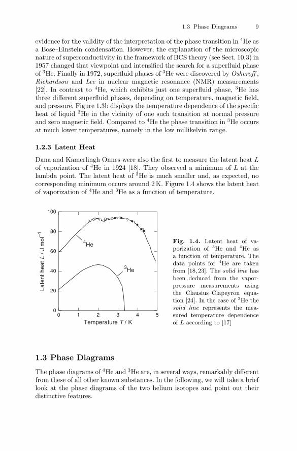
Dana and Kamerlingh Onnes were also the first to measure the latent heat Lof vaporization of 4He in 1924 [18]. They observed a minimum of L at thelambda point. The latent heat of 3He is much smaller and, as expected, nocorresponding minimum occurs around 2 K. Figure 1.4 shows the latent heatof vaporization of 4He and 3He as a function of temperature.
0 1 2 3 4 5Temperature T / K
0
20
40
60
80
100
Late
nthe
atL
/Jm
ol−1
3He
4He Fig. 1.4. Latent heat of va-porization of 3He and 4He asa function of temperature. Thedata points for 4He are takenfrom [18, 23]. The solid line hasbeen deduced from the vapor-pressure measurements usingthe Clausius–Clapeyron equa-tion [24]. In the case of 3He thesolid line represents the mea-sured temperature dependenceof L according to [17]
1.3 Phase Diagrams
The phase diagrams of 4He and 3He are, in several ways, remarkably differentfrom these of all other known substances. In the following, we will take a brieflook at the phase diagrams of the two helium isotopes and point out theirdistinctive features.

10 1 Helium – General Properties
1.3.1 4He
The p–T phase diagram of 4He is shown in Fig. 1.5. It is most remarkablethat helium has no triple point where gas, liquid and solid phase intersect.It remains liquid under normal pressure even at T = 0 as discussed before.Solid helium can only be produced at pressures above 25 bar. Depending ontemperature and pressure one finds three different crystalline modifications.In the whole temperature range – but not at all pressures – solid helium withhcp structure exists. In a small pressure range at temperatures between 1.45 Kand 1.75 K, 4He first solidifies into a bcc structure. For pressures exceeding1 kbar and temperatures above 15 K, 4He shows a fcc phase (not shown inFig. 1.5).
0.1 1 10Temperature T / K
0
10
20
30
40
Pre
ssur
ep
/bar
criticalpoint
Lambda line
solid 4He
4He-II 4He-I
hcp bcc
Fig. 1.5. Phase diagram of 4He [25]
As we have seen before, there are two liquid phases of 4He: helium I andhelium II. The transition from helium I to helium II depends on pressure andis shifted towards lower temperatures with increasing pressure. At the meltingcurve the lambda transition occurs at T = 1.9 K.
At low temperatures (T ≈ 0.8K) the melting curve exhibits a shallowminimum, which is not deep enough to be visible on the scale of Fig. 1.5.Using the Clausius–Clapeyron equation
∂p
∂T
&&&&meltingcurve
=Sℓ − Ss
Vℓ − Vs, (1.5)
we can draw conclusions about the entropies of liquid and solid 4He fromthe melting curve. Here, S and V represent entropy and volume per mole,respectively. The indices ℓ and s denote liquid and solid state, respectively.Since the molar volume of liquid 4He is always larger than that of solid 4He,i.e., Vℓ − Vs > 0, we can conclude from ∂p/∂T < 0 the surprising fact that

1.3 Phase Diagrams 11
below T ≈ 0.8K the entropy of the solid phase is larger than the entropyof the liquid phase. In other words, the disorder in the solid is larger thanin the liquid. The entropy of solid and liquid 4He is determined by thermalexcitations in this temperature range. It turns out that solid 4He has a slightlyhigher phonon heat capacity than liquid 4He, because of the low transversesound velocity in solid 4He. Therefore, at low temperatures the entropy ofsolid 4He is larger than that of liquid 4He.
1.3.2 3He
The phase diagram of 3He (Fig. 1.6) looks qualitatively very similar to thatof 4He, except for the much more pronounced bcc phase. The hcp phase existsin 3He only at pressures above 100 bar. As mentioned before, 3He also exhibitsa transition from a normal fluid to a superfluid phase, or more precisely intothree different superfluid phases. We will return to this point in Chap. 4. Thetransition temperatures are between 1 mK and 3 mK and thus three ordersof magnitude lower than in 4He.
For T → 0, 3He solidifies at pressures above 33 bar. Between 30 and100 bar one finds a bcc structure and above about 100 bar an hcp lattice.The bcc phase in solid 3He is much more extended than in 4He. The reasonis the higher zero-point energy that favors a smaller packing density. Fortemperatures above 18K and for pressures exceeding 1.3 kbar, 3He crystallizesinto a fcc structure. As in 4He, the boundary line between liquid and solid 3He– the melting curve – shows an anomaly at low temperatures, which we willdiscuss in the following section.
Temperature T / K
0
10
20
30
40
Pre
ssur
ep
/bar
criticalpoint
3He-B
3He-A
Tc
solid 3He
normal fluid 3He
bcc
0.001 0.01 0.1 1
Fig. 1.6. Phase diagram of 3He [26]
12 1 Helium – General Properties
Melting Curve
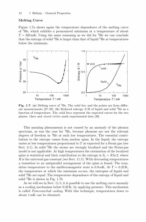
Figure 1.7a shows again the temperature dependence of the melting curveof 3He, which exhibits a pronounced minimum at a temperature of aboutT = 320mK. Using the same reasoning as we did for 4He we can concludethat the entropy of solid 3He is larger than that of liquid 3He at temperaturesbelow the minimum.
10 100 1000Temperature T / mK
25
30
35
40
Pre
ssur
ep
/bar
3He
1 10 100 1000Temperature T / mK
0.0
0.5
1.0
Ent
ropy
S/R
solid
liquid3He
ln(2)
Fig. 1.7. (a) Melting curve of 3He. The solid line and the points are from differ-ent measurements [27–29]. (b) Reduced entropy S/R of liquid and solid 3He as afunction of temperature. The solid lines represent the expected curves for the twophases. Open and closed circles mark experimental data [30]
This amazing phenomenon is not caused by an anomaly of the phononspectrum, as was the case for 4He, because phonons are not the relevantdegrees of freedom in 3He at such low temperatures. The essential contri-bution to the entropy comes from nuclear spins. In the liquid, the entropyvaries at low temperatures proportional to T as expected for a Fermi gas (seeSect. 3.1). In solid 3He the atoms are strongly localized and the Fermi-gasmodel is not applicable. At high temperatures the orientation of the localizedspins is statistical and their contribution to the entropy is Ss = R ln 2, whereR is the universal gas constant (see Sect. 11.5). With decreasing temperaturesa transition to an antiparallel arrangement of the spins is found. The tran-sition temperature to the antiferromagnetic state is 0.9 mK. At T = 0.32 K,the temperature at which the minimum occurs, the entropies of liquid andsolid 3He are equal. The temperature dependence of the entropy of liquid andsolid 3He is shown in Fig. 1.7b
As we will see in Sect. 11.5, it is possible to use the melting curve anomalyas a cooling mechanism below 0.32 K, by applying pressure. This mechanismis called Pomeranchuk cooling. With this technique, temperatures down toabout 1 mK can be obtained.

Exercises 13
Exercises
1.1 Calculate the zero-point energy of a particle in a cube of side length L.Determine the zero-point temperature of H2 , 3He, 4He, Ne and Ar under theassumption that the diameter of the atoms is equal to L.
1.2 Quantum effects are expected to become important if the wavelength ofneighboring atoms noticeably overlap, i.e., if the thermal de Broglie wave-length becomes equal to the interatomic distance. The latter is given ap-proximately by the diameter of the atoms. Calculate the corresponding tem-peratures at which the above condition is met for the systems mentionedin 1.1.
1.3 The latent heat of liquid helium at T = 1 K is L = 2.156 ×10⁶ J m−3 .Calculate the binding energy of a helium atom on the liquid surface.
1.4 Estimate the temperature of the melting-curve minimum for 3He.

2 Superfluid 4He – Helium II
One of the most striking properties of helium II is its ability to flow throughvery small capillaries or narrow channels without experiencing any friction atall. This phenomenon was discovered in 1938 independently by Kapitza [31]and by Allen and his coworker Misener [32]. Kapitza named it superflu-idity in analogy to superconductivity, which denotes the lossless transportof electrons in superconductors. To explain this discovery, F. London sug-gested in 1938 that superfluidity is related to the occurrence of an orderedstate in momentum space, as would be expected for a Bose–Einstein con-densate [33]. Adopting this viewpoint, Tisza postulated in the same year thephenomenological two-fluid model, which nicely describes many propertiesof helium II [34]. A great success of this model was the prediction of secondsound, which was experimentally observed in superfluid helium a few yearslater. Between 1941 and 1947 Landau published three landmark papers ontwo-fluid hydrodynamics, in which he explained the phenomenon of superflu-idity as a consequence of the excitation spectrum of helium II [35]. Finally,Feynman showed that the excitation spectrum postulated by Landau can bederived within a quantum-mechanical description [36].
In this chapter, we shall discuss the extraordinary properties of super-fluid 4He starting with some basic experimental observations, which in par-ticular demonstrate the peculiar behavior of this fascinating liquid. Followingthis we introduce the two-fluid model and discuss whether Bose–Einstein con-densation and the collective excitations proposed by Landau can be used tounderstand the phenomenon of superfluidity, and whether they provide amicroscopic foundation for the two-fluid model.
2.1 Experimental Observations
At high temperatures, liquid 4He behaves as a dense classical gas, but at thelambda point at Tλ = 2.17 K, almost all properties of liquid 4He change. Evenwith the naked eye one can see this dramatic transition. In the normal-fluidstate 4He boils like an ordinary liquid with bubbles rising constantly in theliquid. Below the lambda transition, however, it suddenly becomes deadlyquiet and evaporation only takes place at the free surface of the liquid. In thefollowing we present some additional experimental observations of helium II.

16 2 Superfluid 4He – Helium II
2.1.1 Viscosity and Superfluidity
The first indications for the occurrence of superfluidity came from flow mea-surements through very thin capillaries and narrow slits [31, 32]. Using theHagen–Poiseuille law
V =πr4
81η
∆p
L, (2.1)
one can conclude from measurements of the flow velocity in narrow capillariesthat the viscosity of helium II is several orders of magnitude lower than thatof helium I. The quantity L denotes the length of the capillary, r the radius,∆p the pressure drop along the capillary and V the volume rate of heliumtransported through it. Some measurements that demonstrate the typicalvariation of flow velocity v = V /(πr2 ) with pressure are shown in Fig. 2.1a.Besides the extremely low viscosity, two other very remarkable observationscan be made, namely that the flow velocity is nearly independent of the pres-sure gradient along the capillary, and that the flow velocity increases withdecreasing diameter of the capillary. The temperature dependence of the vis-cosity deduced from flow measurements through narrow capillaries is shownin Fig. 2.1b. Above the lambda point, the viscosity is nearly temperatureindependent, but it falls to an undetectably low value for T < Tλ.
An important question in this context is whether the viscosity becomesextremely small but finite or whether it actually becomes zero below thelambda transition. To answer this question persistent-mass flows have beengenerated and monitored [37,38], analogous to persistent-current experimentswith superconductors (see Chap. 10). A torus, containing compressed finepowder is filled with liquid helium and set into rotation above the lambda
0.00 0.05 0.10 0.15Pressure p / mbar
2
4
6
8
10
12
14
Flo
wve
loci
tyv
/cm
s−1
d = 3.9 µm
d = 0.79 µm
d = 0.12 µm
4He
0 1 2 3 4Temperature T / K
0
10
20
30
Vis
cosi
tyη
/µP
Tλ
4He
Fig. 2.1. (a) Flow velocity of helium II through capillaries with different diameteras a function of the applied pressure [39, 40]. (b) Temperature dependence of theviscosity of liquid helium as determined from flow experiments with thin capillaries

2.1 Experimental Observations 17
point. Because of its viscosity, the helium is dragged along with the torusunder these conditions. The rotating torus is cooled below Tλ and is gentlybrought to rest. Subsequently, the evolution of the angular velocity of the he-lium with time is determined. In several experiments this has been achievedby implementing the torus as part of a superfluid gyroscope. From the obser-vation of a constant angular velocity for many hours one can conclude thatthe viscosity drops at the lambda point by at least eleven orders of magni-tude. Within the accuracy of the experiment, this means that helium II istruly flowing without dissipation.
It has been observed, however, that the results of viscosity measurementson helium II, but not on helium I, depend on the measuring method employed.As we will see later, this very peculiar phenomenon can be explained in theframework of the two-fluid model. Before introducing this model in Sect. 2.2,we will take a brief look at the results obtained with two standard techniquesfor measuring viscosity: the rotary viscosimeter (Fig. 2.2a) and the oscillating-disc method (Fig. 2.2b). In both experiments, the viscosity does not dropinstantaneously to zero at the lambda point but remains finite well below thephase transition. For the rotary viscosimeter, the measured viscosity evenincreases again on cooling below about 1.8 K and substantially exceeds theviscosity of helium I below 1 K. In contrast, η drops steadily below Tλ withdecreasing temperature if measured with an oscillating disc. In addition, inthese experiments with oscillating discs, the damping has quite a strong affecton the amplitude of the oscillation, indicating a nonlinear behavior.
0 1 2 3 4Temperature T / K
0
20
40
60
80
100
Vis
cosi
ty η
/µP
Tλ
4He
0 1 2 3 4Temperature T / K
0
10
20
30
Vis
cosi
tyη
/µP
Tλ
4He
Fig. 2.2. Viscosity of liquid helium as a function of temperature measured (a) witha rotary viscosimeter [41,42] and (b) with an oscillating disc [43]
18 2 Superfluid 4He – Helium II
2.1.2 Beaker Experiments
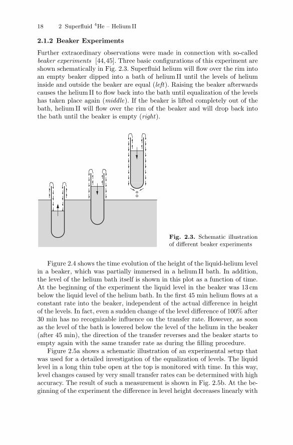
Further extraordinary observations were made in connection with so-calledbeaker experiments [44,45]. Three basic configurations of this experiment areshown schematically in Fig. 2.3. Superfluid helium will flow over the rim intoan empty beaker dipped into a bath of helium II until the levels of heliuminside and outside the beaker are equal (left). Raising the beaker afterwardscauses the helium II to flow back into the bath until equalization of the levelshas taken place again (middle). If the beaker is lifted completely out of thebath, helium II will flow over the rim of the beaker and will drop back intothe bath until the beaker is empty (right).
Fig. 2.3. Schematic illustrationof different beaker experiments
Figure 2.4 shows the time evolution of the height of the liquid-helium levelin a beaker, which was partially immersed in a helium II bath. In addition,the level of the helium bath itself is shown in this plot as a function of time.At the beginning of the experiment the liquid level in the beaker was 13 cmbelow the liquid level of the helium bath. In the first 45 min helium flows at aconstant rate into the beaker, independent of the actual difference in heightof the levels. In fact, even a sudden change of the level difference of 100% after30 min has no recognizable influence on the transfer rate. However, as soonas the level of the bath is lowered below the level of the helium in the beaker(after 45 min), the direction of the transfer reverses and the beaker starts toempty again with the same transfer rate as during the filling procedure.
Figure 2.5a shows a schematic illustration of an experimental setup thatwas used for a detailed investigation of the equalization of levels. The liquidlevel in a long thin tube open at the top is monitored with time. In this way,level changes caused by very small transfer rates can be determined with highaccuracy. The result of such a measurement is shown in Fig. 2.5b. At the be-ginning of the experiment the difference in level height decreases linearly with

2.1 Experimental Observations 19
0 10 20 30 40 50 60 70Time t / min
0
5
10
15
20
25
30H
eigh
th/m
m
Outer levelInner level
Fig. 2.4. Level height of a beaker as afunction of time. The level was 13 cmbelow the surface of the surroundinghelium bath at the beginning of theexperiment [44]
time, which means that the transfer rate is independent of the level differ-ence, as in the experiments discussed previously. But surprisingly, at the timewhen the level difference has almost vanished, an undamped oscillation of thehelium level in the beaker is observed. In the particular experiment discussedhere, the amplitude of this oscillation was about 0.35 mm. The origin of thisoscillation is an overshoot of the flow because of the inertia of the flowinghelium film every time the levels are equal, leading to a periodic reversal ofthe flow. Because of superfluidity the oscillation persists nearly undampedover several minutes in the experiment discussed here. This does not always
Glass
Copper0 1 2 3 4 5 6
Time t / min
0
1
2
3
4
5
Hei
ghth
/mm
Fig. 2.5. (a) Schematic illustration of a beaker experiment that allows a detaileddetermination of the helium transfer. The inner diameter of the tube was only0.58 mm. The copper base of the beaker was incorporated to provide good thermalcontact. For clarity, the helium in the beaker is drawn in light grey, although thereis no difference between the inner and outer helium. (b) Time evolution of thehelium height in the beaker [45]

20 2 Superfluid 4He – Helium II
happen, because, unless special care is taken, temperature gradients betweenthe inside and the outside of the beaker occur, leading to dissipation and thusto a rapid damping of the oscillation.
2.1.3 Thermomechanical Effect
The thermomechanical effect is another unique property of helium II. Aschematic illustration of an experimental setup to observe this effect is shownin Fig. 2.6. Two vessels (A and B), both containing helium II are connectedvia a very thin capillary. Temperature and pressure are equal in both vesselsat the beginning of the experiment and thus the helium levels in the twovessels are the same. Increasing the pressure in A results in a flow of heliumtowards B. Surprisingly, this causes a difference in temperature in the twovessels. The temperature in B decreases somewhat, whereas it increases in A.Equalizing the pressure difference again brings the system back to its startingcondition indicating that this is a reversible process. This experiment clearlyshows that there is mass flow in helium II associated with the heat flow. How-ever, the fact that the direction of heat flow is actually opposite to the flowof mass is very peculiar.
B
∆p
T
∆TT −
A
Fig. 2.6. Schematic illustration of theprinciple of the thermomechanical effect
The reversal of the experiment discussed above, namely generation ofa pressure difference by heating makes possible the observation of a veryattractive phenomenon, the so-called fountain effect (Fig. 2.7). It was firstobserved by Allen and Jones in 1938 in connection with thermal transportmeasurements [46]. The fountain effect can be realized by using a flask witha thin neck immersed in helium at T < Tλ. The lower part of the flask isfilled with a fine compressed powder and is open at the bottom. Above thepowder tablet an electrical heater is located in the flask. Without heating,the flask fills up with helium until the level of the bath is reached. Heatingthe helium in the flask results in a fountain of helium ejected from the topof the flask due to the thermomechanical effect. Stationary fountains withheights up to 30 cm have been achieved in this way. Usually, such fountainsshow turbulent flow. However, under certain conditions (low heater power,

2.1 Experimental Observations 21
HeaterPowder
Fig. 2.7. (a) Schematic sketch of an experimental setup used to demonstrate thefountain effect. The helium inside and outside the flask has been drawn in a slightlydifferent shade for clarity. (b) Photo of a fountain generated in helium II [47]
low temperatures, etc.) fountains can be produced exhibiting pure potentialflow, like the one shown in Fig. 2.7b.
2.1.4 Heat Transport
Early experiments on heat transport in superfluid 4He indicated that thethermal conductivity of helium II is more than five orders of magnitude largerthan that of helium I [48,49]. This extremely high thermal conductivity of thesuperfluid immediately explains the remarkable observation that the boilingof liquid helium stops suddenly when passing the lambda transition. Thetemperature distribution becomes homogeneous within the liquid and thusevaporation takes place only at the free surface.
Not only is the heat transport of helium II very high, it also has a num-ber of other unusual properties. Figure 2.8 shows that under certain cir-cumstances a pronounced maximum of the heat current density is observedat about 1.8 K. Using capillaries with large diameters one finds, in addi-tion, that the heat-current density q rises proportional to |grad T |1/ 3 . Thismeans, that the thermal transport cannot be described by the usual expres-sion q = −Λ gradT , because the thermal conductivity Λ would not be con-stant but would diverge for small temperature gradients as Λ ∝ |gradT |−2 / 3 .
Detailed investigations of the heat flux Q of helium II through very thincapillaries have shown that for small temperature differences the heat flux

22 2 Superfluid 4He – Helium II
1.0 1.5 2.0Temperature T / K
0
1
2
3H
eat-
curr
entd
ensi
tyq•
/Wcm
−2 mK/cm50206310.5
He II
Fig. 2.8. Heat flow in helium IIas a function of temperaturefor different temperature gradi-ents along various capillaries withdiameters between 0.3 mm and1.5 mm [50]
is indeed proportional to grad T as expected. In fact, one finds in helium IIa linear relation between heat flow and temperature gradient in a varietyof different experiments in which the heat flux does not exceed a certaincritical value. The conditions for which this is true is called the linear regime.Results of experiments that exhibit this behavior at low heat flux are shownin Fig. 2.9a. Clearly, the heat flow in these experiments depends linearly onthe temperature gradient for small values and not too high temperatures.
It is important to note that the presence of a linear regime is not only dueto the fact that the nonlinear effects seen at high heat fluxes are small. Thisbecomes clear in Fig. 2.9b in which the thermal resistance ∆T/Q of helium II
0 20 40 60∆T / mK
0
2
4
6
8
Hea
tflo
wQ•
/mW
1.44 K
1.72 K
2.02 KHe II
0 20 40 60 80 100Q
•/ µW
0
20
40
60
∆TQ•
−1/
KW
−1
He II
T = 1.8 K
Fig. 2.9. (a) Heat flow in helium II through a 2.4 µm wide slit as a function ofthe temperature difference ∆T along the slit for three different temperatures [51].(b) Thermal resistance ∆T/Q of helium II in a thin capillary (diameter 107 µm,length 10 cm) as a function of the heat current [52]

2.1 Experimental Observations 23
in a thin capillary is plotted as a function of the heat current. At smallheat currents the thermal resistance is constant, but changes suddenly at acertain value of the heat flux. As we shall discuss later in more detail, the heattransport in helium II is associated with a mass flow for which turbulences inthe liquid arise at a certain critical velocity. This, in turn, leads to a suddenincrease of the thermal resistance.
2.1.5 Second Sound
Temperature waves, which propagate with a characteristic velocity, are an-other very remarkable feature of helium II. Since the propagation of suchwaves is similar to that of ordinary sound this phenomenon was namedsecond sound . The first experimental observation of second sound was madeby Peshkov in 1944. In his early experiments he traced the temperature vari-ation associated with propagating second-sound waves. Later, he improvedthe accuracy of his measurements by generating standing temperature waves.A sketch of his experimental setup for the investigation of standing second-sound waves is shown in Fig. 2.10a.
Using an electrical heater, periodic temperature waves are generated ina resonator with variable length L containing helium II. The temperaturedistribution in the resonator is monitored with a thermometer that can bemoved with respect to the heater position. At resonance, periodic variationsof the temperature in the liquid are observed. The result of measurementsat two different frequencies is shown in Fig. 2.10b, indicating the presenceof standing waves. In this experiment, the velocity of second sound can be
Thermometer
Heater
x
L
-1
0
1 400 Hz
0 5 10 15 20 25Thermometer position x / cm
-4
-2
0
2
4
∆T/a
.u.
96 Hz 1.4 K
Fig. 2.10. (a) Schematic drawing of the apparatus used by Peshkov for the gener-ation and detection of standing temperature waves in helium II. (b) Temperatureof superfluid helium as a function of the thermometer position obtained at twodifferent resonator modes [53]
24 2 Superfluid 4He – Helium II
determined by the simple relation v2 = 2Lν/n for longitudinal resonances.Here, ν denotes the heater frequency and n the number of half-waves in theresonator. With this setup, it is possible to generate temperature waves withfrequencies up to 100 kHz. It is remarkable that the velocity of second soundhas been found to be independent of the frequency of the heat pulses up tothis experimental limit.
2.2 Two-Fluid Model
In this section, we will see that the anomalous properties of helium II can bedescribed phenomenologically with the so-called two-fluid model . The basicidea of this concept was first suggested in 1938 by Tisza, in order to describetransport phenomena of helium II. According to this model, helium II be-haves as if it were a mixture of two completely interpenetrating fluids withdifferent properties, although in reality this is not the case. To avoid anymisunderstanding, it must be clearly stated at the outset that the two flu-ids cannot be physically separated; it is not permissible even to regard someatoms as belonging to the normal fluid and the remainder to the superfluidcomponent, since all 4He atoms are identical. But accepting these limits ofthe physical interpretation, many of the phenomena just described can berelatively clearly understood by formally expressing the density of helium IIas the sum of a normal-fluid and a superfluid component:
ϱ = ϱn + ϱs , (2.2)
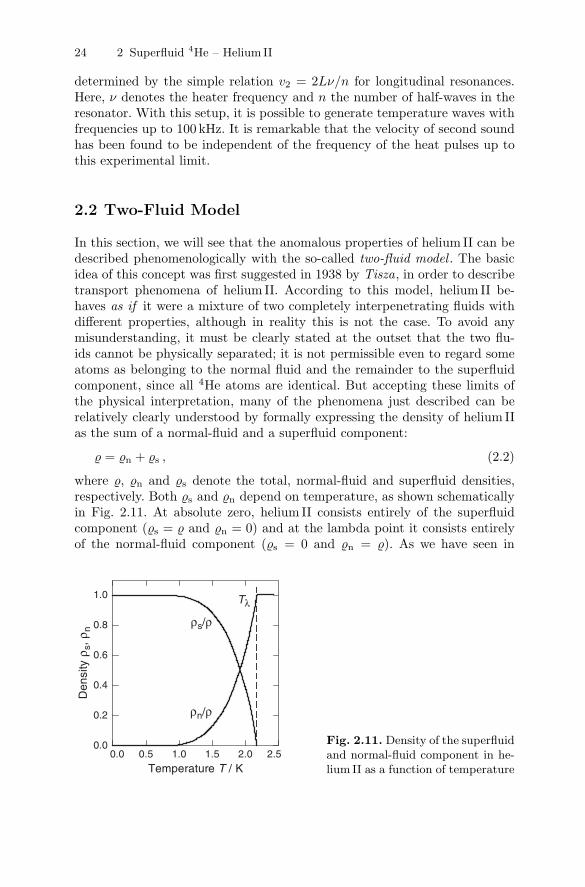
where ϱ, ϱn and ϱs denote the total, normal-fluid and superfluid densities,respectively. Both ϱs and ϱn depend on temperature, as shown schematicallyin Fig. 2.11. At absolute zero, helium II consists entirely of the superfluidcomponent (ϱs = ϱ and ϱn = 0) and at the lambda point it consists entirelyof the normal-fluid component (ϱs = 0 and ϱn = ϱ). As we have seen in
0.0 0.5 1.0 1.5 2.0 2.5Temperature T / K
0.0
0.2
0.4
0.6
0.8
1.0
Den
sity
ρ s,ρ
n
Tλ
ρs/ρ
ρn/ρ
Fig. 2.11. Density of the superfluidand normal-fluid component in he-lium II as a function of temperature

2.2 Two-Fluid Model 25
Sect. 1.2, the total density ϱ is also slightly temperature dependent (seeFig. 1.2). However, in the following description this weak dependence will beneglected. Furthermore, it is assumed that the superfluid component carriesno entropy, exhibits no viscous friction and shows no turbulence. The normal-fluid component, in contrast, is assumed to carry the total entropy of the fluidand to exhibit a finite viscosity. The basic assumptions of the two-fluid modelare summarized in Table 2.1.
Table 2.1. Basic assumptions of the two-fluid model
density viscosity entropy
normal-fluid component ϱn ηn = η Sn = S
superfluid component ϱs ηs = 0 Ss = 0
We shall see that these simple assumptions lead to a satisfying phenom-enological description of many different transport properties of helium II. Af-ter introducing the hydrodynamic equations we shall discuss the experimentalobservations presented in Sect. 2.1 in terms of the two-fluid model.
2.2.1 Two-Fluid Hydrodynamics
In this section, we will look at the basic hydrodynamic equations of the twocomponent fluids. First, we introduce the momentum density j of mass flowper unit volume
j = ϱnvn + ϱsvs . (2.3)
Here, vn and vs denote the velocity of the normal and superfluid component,respectively. Mass conservation is expressed by the continuity equation
∂ϱ
∂t= −div j . (2.4)
Since the viscosity of the normal-fluid component is very low – several ordersof magnitude lower than that of water at 300 K – and its influence in mostexperiments is only a higher-order effect, we shall neglect the normal-fluidviscosity to a first approximation. In this case, helium II is considered as anideal fluid, which can be described by the Euler equation, the equivalent ofNewton’s second law of motion for continua
∂j
∂t+ ϱv · gradv' () *
≈ 0
= −grad p , (2.5)
where p denotes the pressure. If the velocities of the two fluids are not toohigh, to a good approximation we can neglect terms quadratic in the velocitiesas indicated in (2.5).

2.1 Experimental Observations 17
point. Because of its viscosity, the helium is dragged along with the torusunder these conditions. The rotating torus is cooled below Tλ and is gentlybrought to rest. Subsequently, the evolution of the angular velocity of the he-lium with time is determined. In several experiments this has been achievedby implementing the torus as part of a superfluid gyroscope. From the obser-vation of a constant angular velocity for many hours one can conclude thatthe viscosity drops at the lambda point by at least eleven orders of magni-tude. Within the accuracy of the experiment, this means that helium II istruly flowing without dissipation.
It has been observed, however, that the results of viscosity measurementson helium II, but not on helium I, depend on the measuring method employed.As we will see later, this very peculiar phenomenon can be explained in theframework of the two-fluid model. Before introducing this model in Sect. 2.2,we will take a brief look at the results obtained with two standard techniquesfor measuring viscosity: the rotary viscosimeter (Fig. 2.2a) and the oscillating-disc method (Fig. 2.2b). In both experiments, the viscosity does not dropinstantaneously to zero at the lambda point but remains finite well below thephase transition. For the rotary viscosimeter, the measured viscosity evenincreases again on cooling below about 1.8 K and substantially exceeds theviscosity of helium I below 1 K. In contrast, η drops steadily below Tλ withdecreasing temperature if measured with an oscillating disc. In addition, inthese experiments with oscillating discs, the damping has quite a strong affecton the amplitude of the oscillation, indicating a nonlinear behavior.
0 1 2 3 4Temperature T / K
0
20
40
60
80
100
Vis
cosi
ty η
/µP
Tλ
4He
0 1 2 3 4Temperature T / K
0
10
20
30
Vis
cosi
tyη
/µP
Tλ
4He
Fig. 2.2. Viscosity of liquid helium as a function of temperature measured (a) witha rotary viscosimeter [41,42] and (b) with an oscillating disc [43]

18 2 Superfluid 4He – Helium II
2.1.2 Beaker Experiments
Further extraordinary observations were made in connection with so-calledbeaker experiments [44,45]. Three basic configurations of this experiment areshown schematically in Fig. 2.3. Superfluid helium will flow over the rim intoan empty beaker dipped into a bath of helium II until the levels of heliuminside and outside the beaker are equal (left). Raising the beaker afterwardscauses the helium II to flow back into the bath until equalization of the levelshas taken place again (middle). If the beaker is lifted completely out of thebath, helium II will flow over the rim of the beaker and will drop back intothe bath until the beaker is empty (right).
Fig. 2.3. Schematic illustrationof different beaker experiments
Figure 2.4 shows the time evolution of the height of the liquid-helium levelin a beaker, which was partially immersed in a helium II bath. In addition,the level of the helium bath itself is shown in this plot as a function of time.At the beginning of the experiment the liquid level in the beaker was 13 cmbelow the liquid level of the helium bath. In the first 45 min helium flows at aconstant rate into the beaker, independent of the actual difference in heightof the levels. In fact, even a sudden change of the level difference of 100% after30 min has no recognizable influence on the transfer rate. However, as soonas the level of the bath is lowered below the level of the helium in the beaker(after 45 min), the direction of the transfer reverses and the beaker starts toempty again with the same transfer rate as during the filling procedure.
Figure 2.5a shows a schematic illustration of an experimental setup thatwas used for a detailed investigation of the equalization of levels. The liquidlevel in a long thin tube open at the top is monitored with time. In this way,level changes caused by very small transfer rates can be determined with highaccuracy. The result of such a measurement is shown in Fig. 2.5b. At the be-ginning of the experiment the difference in level height decreases linearly with
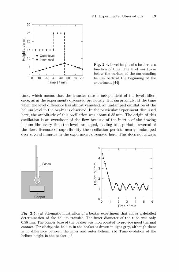
2.1 Experimental Observations 19
0 10 20 30 40 50 60 70Time t / min
0
5
10
15
20
25
30H
eigh
th/m
m
Outer levelInner level
Fig. 2.4. Level height of a beaker as afunction of time. The level was 13 cmbelow the surface of the surroundinghelium bath at the beginning of theexperiment [44]
time, which means that the transfer rate is independent of the level differ-ence, as in the experiments discussed previously. But surprisingly, at the timewhen the level difference has almost vanished, an undamped oscillation of thehelium level in the beaker is observed. In the particular experiment discussedhere, the amplitude of this oscillation was about 0.35 mm. The origin of thisoscillation is an overshoot of the flow because of the inertia of the flowinghelium film every time the levels are equal, leading to a periodic reversal ofthe flow. Because of superfluidity the oscillation persists nearly undampedover several minutes in the experiment discussed here. This does not always
Glass
Copper0 1 2 3 4 5 6
Time t / min
0
1
2
3
4
5
Hei
ghth
/mm
Fig. 2.5. (a) Schematic illustration of a beaker experiment that allows a detaileddetermination of the helium transfer. The inner diameter of the tube was only0.58 mm. The copper base of the beaker was incorporated to provide good thermalcontact. For clarity, the helium in the beaker is drawn in light grey, although thereis no difference between the inner and outer helium. (b) Time evolution of thehelium height in the beaker [45]

20 2 Superfluid 4He – Helium II
happen, because, unless special care is taken, temperature gradients betweenthe inside and the outside of the beaker occur, leading to dissipation and thusto a rapid damping of the oscillation.
2.1.3 Thermomechanical Effect
The thermomechanical effect is another unique property of helium II. Aschematic illustration of an experimental setup to observe this effect is shownin Fig. 2.6. Two vessels (A and B), both containing helium II are connectedvia a very thin capillary. Temperature and pressure are equal in both vesselsat the beginning of the experiment and thus the helium levels in the twovessels are the same. Increasing the pressure in A results in a flow of heliumtowards B. Surprisingly, this causes a difference in temperature in the twovessels. The temperature in B decreases somewhat, whereas it increases in A.Equalizing the pressure difference again brings the system back to its startingcondition indicating that this is a reversible process. This experiment clearlyshows that there is mass flow in helium II associated with the heat flow. How-ever, the fact that the direction of heat flow is actually opposite to the flowof mass is very peculiar.
B
∆p
T
∆TT −
A
Fig. 2.6. Schematic illustration of theprinciple of the thermomechanical effect
The reversal of the experiment discussed above, namely generation ofa pressure difference by heating makes possible the observation of a veryattractive phenomenon, the so-called fountain effect (Fig. 2.7). It was firstobserved by Allen and Jones in 1938 in connection with thermal transportmeasurements [46]. The fountain effect can be realized by using a flask witha thin neck immersed in helium at T < Tλ. The lower part of the flask isfilled with a fine compressed powder and is open at the bottom. Above thepowder tablet an electrical heater is located in the flask. Without heating,the flask fills up with helium until the level of the bath is reached. Heatingthe helium in the flask results in a fountain of helium ejected from the topof the flask due to the thermomechanical effect. Stationary fountains withheights up to 30 cm have been achieved in this way. Usually, such fountainsshow turbulent flow. However, under certain conditions (low heater power,

2.2 Two-Fluid Model 27
2.2.2 Viscosity Measurements
In this section, we shall revisit the viscosity measurements, which have al-ready been presented in Sect. 2.1. Here, we discuss the surprisingly differentresults in the context of the two-fluid model.
Flow Through Thin Capillaries Due to viscous damping the normal-fluidcomponent is almost completely blocked in thin capillaries (vn ≈0). Only thesuperfluid component is mobile and is observed in such experiments. Since itsmotion is frictionless, the measured viscosity is zero below the lambda tran-sition.
Rotary Viscosimeter A rotary viscosimeter consists of two hollow cylin-ders of different size, one rotating inside the other. The viscosity of the liquidbetween the cylinders is determined via the torque Mr = πηωd2
rd2s/(d2
s − d2r )
transferred from the rotating inner cylinder with diameter dr to the outerstationary cylinder with diameter ds. Here, ω denotes the angular velocityof the rotation. Since the viscosity of the superfluid component is zero, itapplies no torque onto the stationary cylinder. Therefore, only the viscosityof the normal-fluid component Mr ∝ η = ηn is measured in such experiments,which is nonzero even below Tλ.
The temperature dependence of ηn is mainly given by the mean freepath ℓn of the thermal excitations in helium. The increase of the mean freepath with decreasing temperature below about 1.8 K can be explained ac-cording to the theory of Landau and Khalatnikov , by the reduction of thescattering of thermal excitations. In their model, they assumed a dilute gas ofexcitations. This assumption is not valid above 1.8 K and therefore the tem-perature dependence of the normal-fluid viscosity in this temperature rangecannot be explained with this theory.
Oscillating-Disc Viscosimeter The viscosity measurements made withthis technique are based on the torque Md = π
√ϱη ω3 / 2 r4 Θ(ω) acting on an
oscillating disc with radius r in the liquid. Here, Θ(ω) = Θ0 cos(ωt − π/4)denotes the angle of deflection and ω the angular frequency of the oscillation.The crucial point is that, in this experiment, it is not just the viscosity thatis measured, but the product ϱ η of density and viscosity.
Since the superfluid component does not contribute below Tλ (ηs = 0), theapparent viscosity is given by ϱnηn. Therefore, the temperature dependenceshown in Fig. 2.5 is understandable because the density of the normal-fluidcomponent decreases rapidly below the lambda point. Using the result for ηn
from the measurement with rotary viscosimeters, it is possible to draw conclu-sions about the temperature dependence of ϱn. The first direct measurementof this quantity is discussed in the next section.

28 2 Superfluid 4He – Helium II
2.2.3 Determination of ϱn/ϱ
A schematic drawing of the specially designed torsion oscillator that An-dronikashvili used in 1948 to determine the normal-fluid density ϱn is shownin Fig. 2.12 [55]. The torsion pendulum consisted of 50 equally spaced alu-minum discs with a diameter of 3.5 cm and a thickness of only 13µm. Thediscs were mounted on a rod separated from each other by 210µm. The rodwith the discs was suspended by a torsion fiber forming an oscillator. Thelower part of the oscillator was immersed in liquid helium. In the actual ex-periment, slow oscillations with a typical period of 30 s were excited and theresulting deflection amplitude was detected optically via a mirror that wasrigidly attached to the axis of the pendulum.
Window
Mirror
Liquid Helium
Al−discs
To pump
Fig. 2.12. Schematic drawing of the appara-tus used by Andronikashvili to determine thenormal-fluid density ϱn of helium II
The total mass of the pendulum bob determines its moment of inertia.The oscillator was driven at the resonant frequency of its torsional mode. Thisfrequency depends on the ratio of the torsion constant and the moment ofinertia of the pendulum. The discs of the viscosimeter were constructed fromvery light material to achieve as large a change as possible in the moment ofinertia for a given change of the entrained mass. The spacing d between thediscs and the period of oscillation were chosen so that the viscous penetrationdepth δ =
+2ηn/ϱnω was larger than the distance between the aluminum
discs throughout the entire experiment. Therefore, the complete normal-fluidcomponent ϱn, but not the superfluid component ϱs, was dragged with thediscs above and below the lambda point.
In this way, the temperature dependence of ϱn can be measured directly.The results of the original measurements by Andronikashvili are shown inFig. 2.13. Above Tλ, all the fluid is dragged with the discs and the datareflect the temperature dependence of the density of helium I. Below Tλ,

2.2 Two-Fluid Model 29
1.5 2.0 2.5 3.0 3.5Temperature T / K
0.0
0.2
0.4
0.6
0.8
1.0ρ n
/ρλ
TλHe II
Fig. 2.13. Temperature dependenceof the normal-fluid density ϱn normal-ized to the density ϱλ at Tλ. Thedata were obtained with two differentmethods: Andronikashvili viscosime-ter, and • second-sound measurements(after [56])
however, the period of oscillation decreases sharply, indicating that the fluidin the spaces was not completely entrained by the discs. This result confirmsthe prediction that the superfluid component has no effect on the torsionpendulum. The temperature dependence of ϱn below the lambda point canbe described by the empirical formula
ϱn = ϱλ
,T
Tλ
-5 .6
, (2.11)
where ϱλ denotes the density at the lambda point. For comparison, thenormal-fluid density ϱn as determined by second-sound measurements is alsoshown in Figure 2.13. As can be seen, the results of the two methods are invery good agreement. In more recent experiments, the ratio ϱs/ϱ has beendetermined over a wider temperature range (see Sect. 2.5).
2.2.4 Beaker Experiments
The explanation of the peculiar behavior of helium II in the beaker experi-ments is straightforward. The geometrical conditions on which we base ourconsiderations are shown in Fig. 2.14. A helium film forms on surfaces abovea bath of helium II. The Van der Waals force between helium atoms and thewalls plays a crucial role here. The properties of such helium films can bediscussed in a simple way in terms of the chemical potential µ. For films insaturated vapor and thermodynamic equilibrium we have
µf = µg = µℓ . (2.12)
Here, the indices f, g and ℓ refer to film, gas and liquid.The fact that the film is located on the beaker walls above the liquid
surface indicates that the influence of gravity is compensated by Van derWaals forces. Therefore, we can write
µf = µℓ +µgrav + µvdW' () *= 0
= µℓ . (2.13)

52 2 Superfluid 4He – Helium II
2.4 Macroscopic Quantum State
F. London repeatedly stressed in different publications that the condensateis a quantum state on a macroscopic scale [11]. Later, this viewpoint wasextended to the whole superfluid component since it is assumed that the con-densate and the superfluid component are closely related. As we will see, thepresence of a macroscopic quantum state has consequences for the propertiesof helium II. For example, it results in a quantization of circulation and itenables phenomena analogous to the Josephson effect in superconductors.
2.4.1 Wave Function of the Superfluid Component
The macroscopic quantum state present in helium II can be described by thewave function
ψ(r) = ψ0 eiϕ(r) , (2.67)
where the phase ϕ(r) is a real-valued function of the position. The ampli-tude ψ0 is constant or, under certain conditions, just slightly position de-pendent. Henceforth, we shall omit the position dependence. The absolutevalue of the wave function is given by the number of atoms in the superfluidcomponent per unit volume and can be expressed by
ψ⋆ψ = |ψ0 |2 =ϱs
m4. (2.68)
Here, m4 denotes the mass of 4He atoms. The phase of the macroscopic waveis related to the velocity of atoms. The momentum p of a helium atom in thesuperfluid component can be described with the Schrodinger equation
−i!∇ψ = p ψ . (2.69)
Using (2.67) we find p = !∇ϕ(r) = m4vs and thus
vs =!m4
∇ϕ(r) . (2.70)
The velocity of the superfluid component therefore determines the phaseshift of the wave function. The phase is constant for vs = 0, and changesuniformly for vs = const. The phase of the wave function is a well-definedquantity within the entire liquid. We can think of particles being ‘rigidly’connected, though it should be emphasized that this rigid coupling takesplace in momentum space and not in real space. This concept can be verifiedby investigating helium II under rotation. Corresponding experiments will bediscussed in the following section.
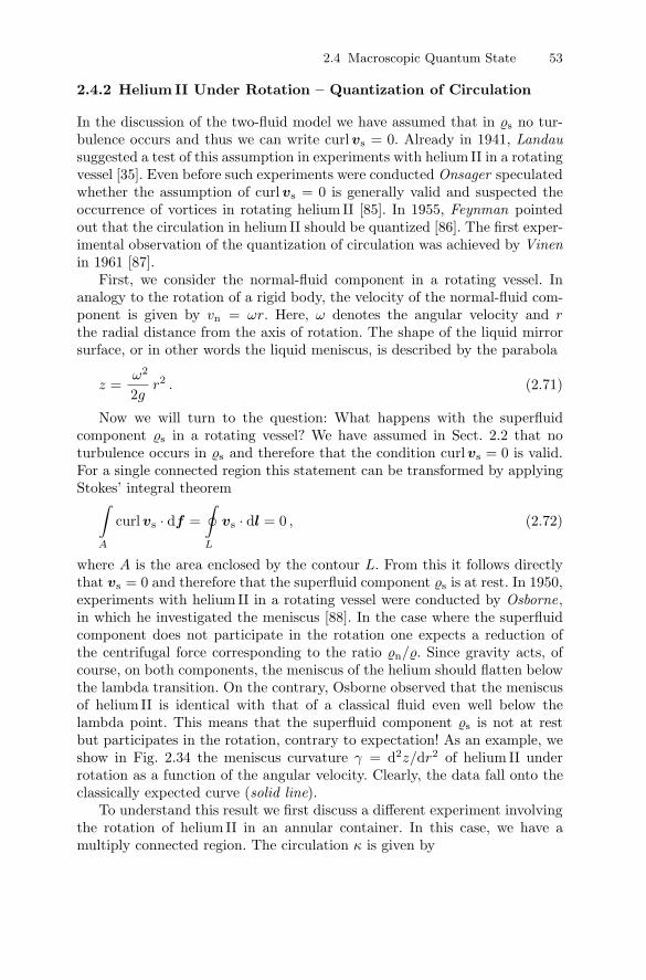
2.4 Macroscopic Quantum State 53
2.4.2 Helium II Under Rotation – Quantization of Circulation
In the discussion of the two-fluid model we have assumed that in ϱs no tur-bulence occurs and thus we can write curlvs = 0. Already in 1941, Landausuggested a test of this assumption in experiments with helium II in a rotatingvessel [35]. Even before such experiments were conducted Onsager speculatedwhether the assumption of curlvs = 0 is generally valid and suspected theoccurrence of vortices in rotating helium II [85]. In 1955, Feynman pointedout that the circulation in helium II should be quantized [86]. The first exper-imental observation of the quantization of circulation was achieved by Vinenin 1961 [87].
First, we consider the normal-fluid component in a rotating vessel. Inanalogy to the rotation of a rigid body, the velocity of the normal-fluid com-ponent is given by vn = ωr. Here, ω denotes the angular velocity and rthe radial distance from the axis of rotation. The shape of the liquid mirrorsurface, or in other words the liquid meniscus, is described by the parabola
z =ω2
2gr2 . (2.71)
Now we will turn to the question: What happens with the superfluidcomponent ϱs in a rotating vessel? We have assumed in Sect. 2.2 that noturbulence occurs in ϱs and therefore that the condition curlvs = 0 is valid.For a single connected region this statement can be transformed by applyingStokes’ integral theorem
%
A
curlvs · df =.
L
vs · dl = 0 , (2.72)
where A is the area enclosed by the contour L. From this it follows directlythat vs = 0 and therefore that the superfluid component ϱs is at rest. In 1950,experiments with helium II in a rotating vessel were conducted by Osborne,in which he investigated the meniscus [88]. In the case where the superfluidcomponent does not participate in the rotation one expects a reduction ofthe centrifugal force corresponding to the ratio ϱn/ϱ. Since gravity acts, ofcourse, on both components, the meniscus of the helium should flatten belowthe lambda transition. On the contrary, Osborne observed that the meniscusof helium II is identical with that of a classical fluid even well below thelambda point. This means that the superfluid component ϱs is not at restbut participates in the rotation, contrary to expectation! As an example, weshow in Fig. 2.34 the meniscus curvature γ = d2z/dr2 of helium II underrotation as a function of the angular velocity. Clearly, the data fall onto theclassically expected curve (solid line).
To understand this result we first discuss a different experiment involvingthe rotation of helium II in an annular container. In this case, we have amultiply connected region. The circulation κ is given by
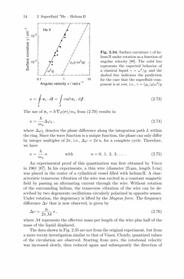
54 2 Superfluid 4He – Helium II
0.1 1 10Angular velocity v / rad s−1
10-4
10-3
Sur
face
curv
atur
eγ
/cm
−1
ω2/g
ρn/ρ (ω2/g)
He II
Fig. 2.34. Surface curvature γ of he-lium II under rotation as a function ofangular velocity [89]. The solid linerepresents the expected behavior ofa classical liquid γ = ω2/g, and thedashed line indicates the predictionfor the case that the superfluid com-ponent is at rest, i.e., γ = (ϱn/ϱ)ω2/g
κ =.
L
vs · dl =%
A
curlvs · df . (2.73)
The use of vs = !∇ϕ(r)/m4 from (2.70) results in
κ =!
m4∆ϕL , (2.74)
where ∆ϕL denotes the phase difference along the integration path L withinthe ring. Since the wave function is a unique function, the phase can only differby integer multiples of 2π, i.e., ∆ϕ = 2π n, for a complete cycle. Therefore,we have
κ =h
m4n with n = 0, 1, 2, 3, . . . . (2.75)
An experimental proof of this quantization was first obtained by Vinenin 1961 [87]. In his experiments, a thin wire (diameter 25µm, length 5 cm)was placed in the center of a cylindrical vessel filled with helium II. A char-acteristic transverse vibration of the wire was excited in a constant magneticfield by passing an alternating current through the wire. Without rotationof the surrounding helium, the transverse vibration of the wire can be de-scribed by two degenerate oscillations circularly polarized in opposite senses.Under rotation, the degeneracy is lifted by the Magnus force. The frequencydifference ∆ν that is now observed, is given by
∆ν =ϱs
2πM κ , (2.76)
where M represents the effective mass per length of the wire plus half of themass of the liquid displaced.
The data shown in Fig. 2.35 are not from the original experiment, but froma more recent investigation similar to that of Vinen. Clearly, quantized valuesof the circulation are observed. Starting from zero, the rotational velocitywas increased slowly, then reduced again and subsequently the direction of

2.4 Macroscopic Quantum State 55
rotation was reversed. During this sequence distinctive hysteretic effects werevisible. In such experiments, indications for a quantization up to n = 4 havebeen found (not shown in Fig. 2.35).
-4 -2 0 2 4Angular velocity Ω / rad s−1
-4
-2
0
2
4
Circ
ulat
ion
κ/h
m4−1
Fig. 2.35. Circulation κ in units of h/m4 as a function of the angular velocityof the rotating cylinder. The arrows indicate the sequence in which the angularvelocity was changed [90]
Vortices with Quantized Circulation
We have seen that in a multiply connected region the circulation of the su-perfluid component can be finite and that its magnitude is quantized. Nowwe come back to the question why the superfluid component seems to partic-ipate in the rotation in singly connected regions. The reason is that vorticesoccur under rotation having a normal-fluid core so that no singly connectedregion exists within the superfluid component. The occurrence of vortices inhelium II therefore provides the explanation for the ‘classical’ meniscus ob-served in Osborne’s experiments. A schematic illustration of the situation isshown in Fig. 2.36a.
The occurrence of a normal-fluid core in such vortices can be made plau-sible in the following way. As in a vortex in a classical liquid, the velocityof the superfluid component rises proportional to 1/r with decreasing dis-tance r from the center of the vortex. As soon as the critical velocity is ex-ceeded, superfluidity breaks down and a normal-fluid region is formed. Theradial dependence of ϱs/ϱ and vs in the vicinity of a vortex core is shown inFig. 2.36b. Using classical hydrodynamics and (2.75) one finds for the velocityof the superfluid component:
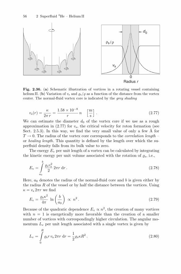
56 2 Superfluid 4He – Helium II
d0
0
sv
sρ ρ/
Radius r
Fig. 2.36. (a) Schematic illustration of vortices in a rotating vessel containinghelium II. (b) Variation of vs and ϱs/ϱ as a function of the distance from the vortexcenter. The normal-fluid vortex core is indicated by the grey shading
vs(r) =κ
2π r=
1.58 ×10⁻⁸
rn
/ms
0. (2.77)
We can estimate the diameter d0 of the vortex core if we use as a roughapproximation in (2.77) for vs, the critical velocity for roton formation (seeSect. 2.5.3). In this way, we find the very small value of only a few A forT → 0. The radius of the vortex core corresponds to the correlation length –or healing length. This quantity is defined by the length over which the su-perfluid density falls from its bulk value to zero.
The energy Ev per unit length of a vortex can be calculated by integratingthe kinetic energy per unit volume associated with the rotation of ϱs, i.e.,
Ev =b%
a0
ϱsv2s
22πr dr . (2.78)
Here, a0 denotes the radius of the normal-fluid core and b is given either bythe radius R of the vessel or by half the distance between the vortices. Usingκ = vs 2πr we find
Ev =ϱsκ2
4πln
,b
a0
-∝ n2 . (2.79)
Because of the quadratic dependence Ev ∝ n2 , the creation of many vorticeswith n = 1 is energetically more favorable than the creation of a smallernumber of vortices with correspondingly higher circulation. The angular mo-mentum Lv per unit length associated with a single vortex is given by
Lv =R%
0
ϱsr vs 2πr dr =12ϱsκR2 . (2.80)

2.4 Macroscopic Quantum State 57
It can be shown that the critical angular velocity ωc for the formation of thefirst vortex is given by the condition ωc = Ev/Lv (see, for example, [91])resulting in
ωc =h
2πm4R2ln
,R
a0
-. (2.81)
For R = 1 cm, we find the small critical angular velocity ωc ≈10−3 s−1.The presence of vortices can be shown via electrons trapped in the vortex
cores. As we will see in the following section, free electrons create bubblesin helium. Because of the circulation and the action of Bernoulli forces theelectrons are captured by the vortex cores. By applying an electric field par-allel to the vortex lines, the electrons are pulled along the vortices to thesurface and the charge accumulating at the surface can be measured withan electrometer. Under the assumption that the electrons are captured atconstant rate, the voltage at the electrometer is proportional to the numberof vortices present at a given time. If a new vortex is formed upon increasingthe angular velocity, the electrometer signal jumps to a higher value. Theresult of such an experiment is shown in Fig. 2.37. The nature of this data issomewhat analogous to the measurement of quantized magnetic flux lines intype II superconductors (see Sect. 10.1.4). In fact, there are a number of otheranalogies between these two phenomena. Just as in vortices, the cores of theflux tubes in superconductors are normal conducting. In addition, we find inboth cases a regular spatial arrangement, the so-called Abrikosov lattice.
A very impressive direct visualization of the vortex lattice is possible byaccelerating the captured electrons with an electric field and having themhit a phosphorescent screen. In Fig. 2.38 the results of such a measurement
1.4 1.6 1.8 2.0 2.2Angular velocity Ω / rad s−1
0
1
2
3
Ele
ctro
met
ersi
gnal
/V He II
Fig. 2.37. Electrometer signal as a function of angular velocity. The velocity ofrotation of the helium II was increased steadily in this experiment [92]

58 2 Superfluid 4He – Helium II
Fig. 2.38. Visualization of quantized vortices in rotating helium II of 0.1 K [93,94]
are shown. In this experiment, the helium II was located in a rotating vessel,2 mm in diameter and 25 cm long. The angular velocities were in the rangebetween 0.3 and 0.8 rad s−1. The image was transferred out of the cryostat byoptical fibers, amplified and photographed. With increasing angular velocitythe number of vortices increases as expected. The regular arrangement of thevortices is evident.
2.4.3 Josephson Effect
In 1962, Josephson predicted that if two superconductors are separated by athin insulator, the superposition of the wave functions of the bulk supercon-ductors causes a current crossing the junction that depends sinusoidally onthe phase difference [95] (see also Sect. 10.4.2). This is a direct consequenceof the macroscopic nature of the wave function in superconductors. Since thesuperfluid component of helium II can also be described by a macroscopicwave function one expects analogous phenomena to occur for the mass flowof helium II through a microscopic aperture, providing a so-called weak linkbetween two vessels containing helium II. The size of the aperture has to beof the order of the healing length. Since, at low temperatures, the healinglength is extremely small for helium II (ξ = 1 . . . 2 A), it is experimentallyvery difficult to achieve this condition. However, since the healing length di-verges for T → Tλ (see Sect. 2.6) one can meet the required condition byperforming measurements very close to the lambda transition.