Low-latency histogram equalization for infrared image … · 2011-06-26 · Low-latency histogram...

1

Low-latency histogram equalization for infraredimage sequences – a hardware implementationVolker SchatzFraunhofer Institut fur Optronik, Systemtechnik und Bildauswertung, Ettlingen, Germanyfirstname.lastname∂iosb.fraunhofer.de

This is the author-generated version of a paper published in the Journal of Real-Time Image Processing on 15 June2011 (received 22 November 2010, accepted 13 May 2011).

As per the copyright transfer agreement, this document must contain the following notice and hyperlink:“The final publication is available at www.springerlink.com”

This author’s version has been enhanced by oversized internal links and citation classes and contains the resultimages in their full resolution.

This work describes a hardware implementation of thecontrast-limited adaptive histogram equalization algorithm(CLAHE). The intended application is the processing ofimage sequences from high-dynamic-range infrared cameras.The variant of histogram equalization implemented is theone most commonly used today. It involves dividing theimage into tiles, computing a transformation function oneach of them, and interpolating between them. The contrast-limiting is modified to facilitate the hardware implemen-tation, and it is shown that the error introduced by thismodification is negligible. The latency of the design isminimized by performing its successive steps simultaneouslyon the same frame and by exploiting the vertical blankpause between frames. The resource usage of the histogramequalization module and how it depends on its parametershas been determined by synthesis. The design has beensynthesized and tested on a Xilinx FPGA. The implemen-tation supports substituting other dynamic range reductionmodules for the histogram equalization component by partialdynamic reconfiguration.

Keywords: Histogram equalization, CLAHE, infrared images,FPGA design, partial dynamic reconfiguration

1 INTRODUCTION

Histogram equalization is an image enhancement tech-nique that consists in a grey-level transform designedto equalize the frequency of occurrence of differentgrey values. It has its origins in the information the-oretic problem of maximizing the information contentof discretized data by applying a transformation beforediscretization. These concepts were applied to imagesby Hummel [Hum75]. Histogram equalization has sincebeen successively refined. Most importantly, each pixelcan be transformed based on the histogram of a con-textual region [KLW74, KLW76, Hum77, Piz81], and thecontrast amplification can be limited by clipping thehistogram [PAA+87]. The latter variant, called contrast-limited adaptive histogram equalization (CLAHE), is inmost widespread use today and is the method that hasbeen implemented here.

Specialized hardware for computing histogram equal-ization also has a long history. The paper that intro-duced contrast limiting [PAA+87] also discussed how to

implement histogram equalization on special processorarchitectures. Since then, implementations as a special-ized multiprocessor machine [EPA90] and as parallelsoftware on commercially available hardware [Kur91]have been provided. More recently, several implementa-tions of global histogram equalization have been devel-oped that either partly [SS99, DND+01] or exclusively[LNC+98, JCR03, AA05] rely on FPGA logic. Reza haspresented a hardware implementation of CLAHE withan application in medical imaging in mind [Rez04].Ferguson et al. have developed an FPGA implementationof CLAHE intended for video processing [FAEP08]. Bothclosely follow the software algorithm.

The intended application of this implementation isthe processing of image sequences from an infrared (IR)camera with a dynamic range of 14 bits or more. Reduc-ing the dynamic range is necessary before the imagescan be displayed on a standard computer monitor. Mostdisplays support a dynamic range of 8 bits in eachcolour channel, resulting in a dynamic range of 8 bitsfor greyscale images as well. Displays with a higherdynamic range are sometimes recommended, such asfor medical applications [NEM09], but the availabledynamic range should always be utilized as effectivelyas possible. Histogram equalization is the method ofchoice for this purpose.

Besides visualization, there are other reasons to usehistogram equalization. The FPGA implementation thatis presented in this paper is to be part of a reconfigurablehardware image processing system briefly described in[BGP+09]. Reducing the dynamic range of pixel valuesallows to reduce the chip area required for downstreamimage processing algorithms if necessitated by resourceconstraints. Employing histogram equalization for thispurpose allows to do this in a way that minimizes imagedegradation. As one important application of the imageprocessing system is the investigation of object trackingmethods, an important requirement for this histogramequalization implementation is minimal latency, so thatthe reaction time of tracking algorithms is largely unaf-fected.

Author-generated version of DOI 10.1007/s11554-011-0204-y published in the Journal of Real-Time Image Processing

http://www.springerlink.com/openurl.asp?genre=article&id=doi:10.1007/s11554-011-0204-y

http://dx.doi.org/10.1007/s11554-011-0204-y

2 Volker Schatz: Low-latency histogram equalization for infrared image sequences – a hardware implementation

This paper is structured as follows. The followingsection will review histogram equalization methods andpresent an optimization of the chosen method for ahardware implementation. The implementation will bepresented in section 3 and the appendix. Section 4 willdescribe the application and the test setup and demon-strate the benefits of partial dynamic reconfiguration.The final section will summarize the paper.

2 THEORY

2.1 Transformation formulaThis section will present a brief derivation of the his-togram equalization transformation formula; for a moredetailed version, see [Hum75] or textbooks such as[GW02].

Histogram equalization, as its name suggests, refersto transforming an image in such a way that the his-togram of the resulting image is flat. It is not generallypossible to do this exactly in the case of a real-worlddiscretized image. In the following derivation, we willtherefore work with an idealized greyscale image, whichhas continuous coordinates and a continuous brightnessvalue at each point. Without loss of generality, we willassume the range of brightness values is the unit intervalI = [0, 1].

Then the histogram of the image is also a continuousfunction, the probability density function (PDF) of theimage values x:

p : I → I

x 7→ p(x)

If y is the image value x is transformed to, and q isits PDF, the requirement of histogram equalization isexpressed by q(y) ≡ 1. From the principle of probabilityconservation

|p(x) dx| = |q(y) dy|

and the requirement that we seek a monotonically in-creasing transformation function, one derives the trans-formation:

y =

∫ x

0

p(x′) dx′

Expressed in words, the histogram equalizing transfor-mation function is the cumulative distribution function(CDF) of the image values.

This transformation formula is discretized for use withreal-world discretized images:

x ∈ {0, 1, . . . , 2ξ − 1}y ∈ {0, 1, . . . , 2η − 1}

y =

⌊2η − 1

N

x∑x′=0

Nx′

⌋, (1)

where N is the total number of pixels in the image orimage region, Nx is the number of pixels with value x,and b·c is the floor function. Usually ξ ≥ η, i.e., y has

no more bits than x. If some of the bin counts Nx′ aretoo large (larger than N/(2η − 1)), there will be gapsin the histogram of y. This is a consequence of thefact that values that have been lumped together in thesame x bin cannot be picked apart again. So in thediscretized case, the histogram of the image resultingfrom a histogram equalization is only flat when averagedacross the gaps. Nonetheless, the resulting image showsimproved contrast.y can also be computed from a histogram that contains

more than one value of x in each bin. This requiresthat the bit width of y is smaller than that of x, or theaccuracy of the result will suffer. The formula for y thentakes the form:

y =

2η − 1

N

β(x)∑b=0

Nb

, (2)

where Nb is the bin count of bin b and β(x) stands forthe bin which the original pixel value x belongs to.

2.2 Variants

Since its inception, histogram equalization has evolvedinto a number of variants, each of which redressessome of the drawbacks of the previous one. Applyinghistogram equalization globally to an image has thedisadvantage that bright and dark regions of the imageare treated equally. This may cause the contrast invery bright or dark regions to remain bad or evento deteriorate. This problem is solved by adaptivehistogram equalization (AHE) [KLW74, KLW76, Hum77,Piz81]. AHE transforms each pixel according to thehistogram of a neighbourhood region. As a consequence,contrast is enhanced locally, with physically separatedbright and dark regions treated independently. The sizeof the neighbourhood region serves as a scale parameter.Variations in the image data on length scales larger thanthis parameter are suppressed, those on smaller lengthscales are enhanced.

The downside of AHE from a quality perspective isthat it can overamplify noise: when the neighbourhoodlies completely within a nearly homogeneous region,a very small range of values is mapped to the wholeoutput range. This is remedied by CLAHE [PAA+87].This method clips the histogram at a predeterminedvalue before computing the transformation function,thereby limiting the contrast amplification. It was found[PAA+87] that it is advantageous to redistribute theexcess rather than discard it. This is done in a re-cursive process that, while it can be implemented inhardware [Rez04, FAEP08], is not particularly suitablefor it. The following subsection will present an equallygood alternative that lends itself well to a hardwareimplementation.

The second drawback of AHE (and the straightfor-ward version of CLAHE) is that it is computationallyexpensive (in software) or quite complex (in hardware).


http://dx.doi.org/10.1007/s11554-011-0204-y

Volker Schatz: Low-latency histogram equalization for infrared image sequences – a hardware implementation 3

��

��

��

��

��

(a) (b) (c)

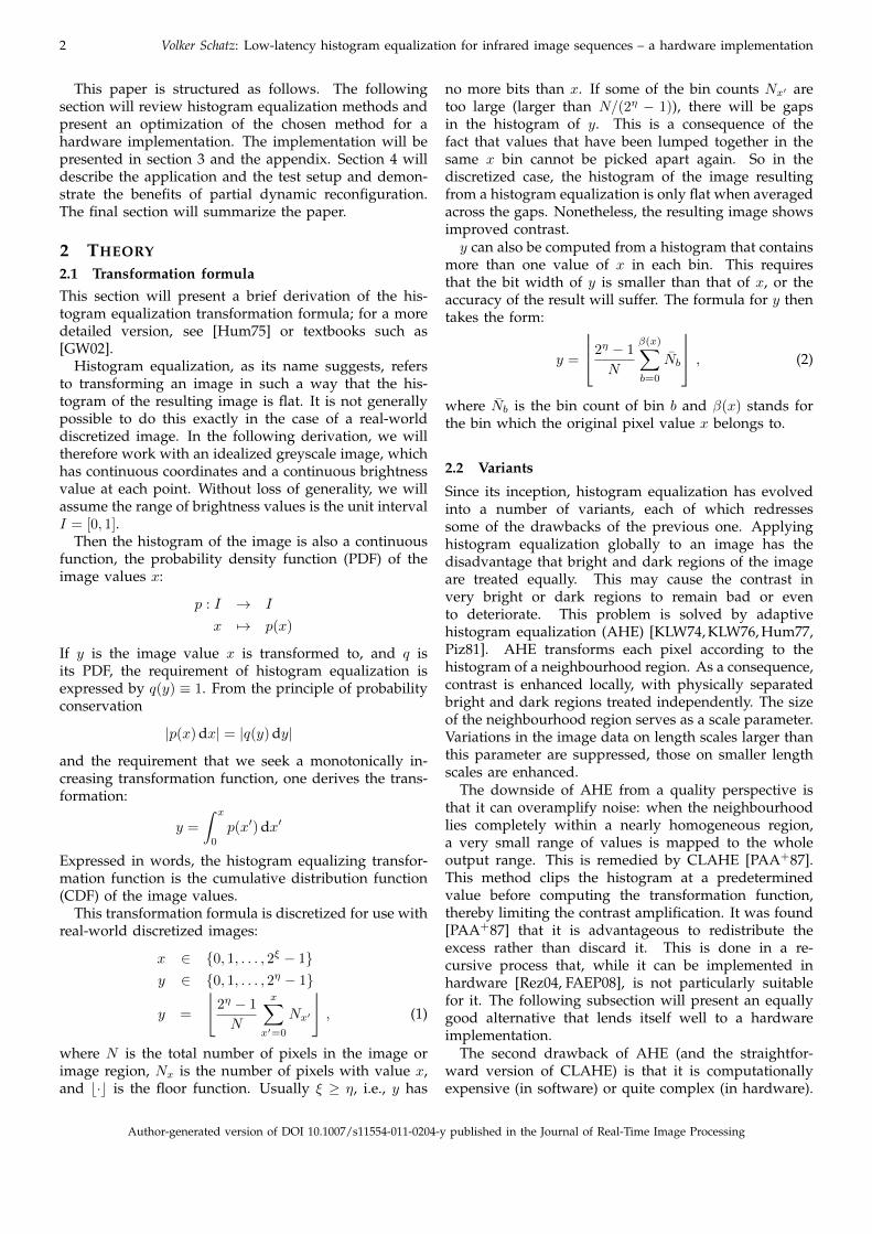
Figure 2. The redistribution procedure that is part of the histogram clipping for CLAHE. (a), (b) One step in the conventional recursive method.(c) The new single-step method: only non-exceeding bins receive the redistributed excess, and the secondary excess is discarded (see text).

c

ab

b

Figure 1. Tile-interpolated CLAHE: Transformations computed fromthe tile histograms are appropriate for the tile centre pixels (blacksquares). Pixels in the bulk of the image (a) are bilinearly, margin pixels(b) linearly interpolated between the transformations of the nearestcentre pixels. Corner pixels (c) transform as the corner centre pixel.

This is also redressed in [PAA+87]. Rather than computethe histograms and transformation functions for theneighbourhood of each pixel, this is done for each tileof a rectangular grid into which the image is dividedup. For the centre pixel of a tile, that transformationfunction is obviously the correct one. For the others, alinear interpolation between the transforms belonging tothe nearest tile-centre pixels is performed as displayedin figure 1. Most pixels lie in the bulk of the imageand are surrounded by four tile centre pixels. They aretransformed with the corresponding four different trans-formation functions and interpolated bilinearly to obtainthe result pixel value. Pixels on the image marginsare linearly interpolated between transformation resultsfrom the two neighbouring centre pixel transformationfunctions. Finally, corner pixels are not interpolated at allbut simply transformed with the transformation functionof their tile.

2.3 Excess redistribution without recursion

The key element of CLAHE is the limiting of the contrastamplification by clipping the histogram before comput-ing the transformation function. The conventional wayof doing this is by the following recursive procedure

[PAA+87]. The histogram is clipped at the predefinedclip limit, which is a parameter of CLAHE. The totalexcess from those bins that exceed the clip limit isdistributed equally over all histogram bins, as depictedin figure 2. This once again pushes some bin countsover the clip limit (figure 2 (b)). The resulting excess isredistributed again, and the procedure is repeated untilthe limit is not exceeded by any bin any more.

Implementing recursion in hardware can be complex,necessitating the implementation of control flow and ofstorage for intermediate results, and time-consuming, asrecursions are performed sequentially. In particular, inour case each recursion requires a complete pass overthe histogram RAM even if redistributing the excess anddetermining the excess for the next round are combined[Rez04]. This means that the time for the whole redis-tribution procedure is of the order of the number ofiterations times the number of histogram bins.

Fortunately, the redistribution can be well approxi-mated by a single-step procedure. It is based on theobservation that the histogram bins that initially exceedthe clip limit will again do so in every recursion. This isbecause those bins are clipped to exactly the clip limit, soevery redistribution step will push them over the limitagain. What is more, only a few additional bins will beclipped in the later recursions, namely those that do notinitially exceed the limit but are close enough to it that aredistribution step makes them exceed it. The single-stepredistribution procedure then consists of redistributingthe initial excess only once, and only among the bins thatdo not initially exceed the limit, as displayed in figure 2(c). The relatively few bins that are pushed over the limitare clipped again, and the secondary excess, marked byred crosses in figure 2 (c), is discarded.

2.4 Validity of the approximationThe following calculation will estimate the error incurredby discarding the secondary excess. To that end, we willutilize the continuous formulation introduced in the firstpart of section 2.1. Since the histograms of IR imagesconsist of one or several peaks (see figure 3), a Gaus-sian function will be used as an exemplary continuoushistogram.

It seems unlikely that the precise shape of the peakwould influence the error introduced by the modified


http://dx.doi.org/10.1007/s11554-011-0204-y


0

100

200

300

400

500

600

0 2048 4096 6144 8192 10240 12288 14336 16384

Fre

qu

en

cy

Pixel value

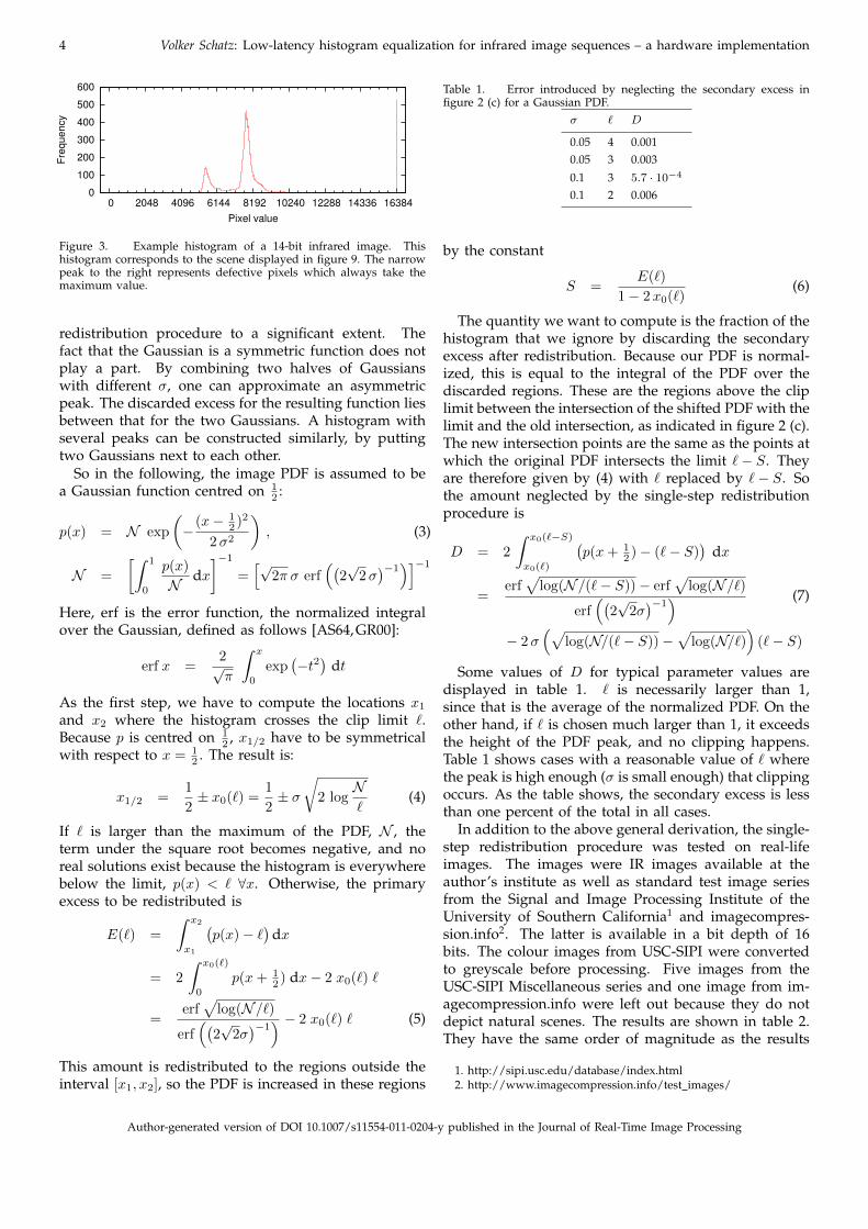
Figure 3. Example histogram of a 14-bit infrared image. Thishistogram corresponds to the scene displayed in figure 9. The narrowpeak to the right represents defective pixels which always take themaximum value.

redistribution procedure to a significant extent. Thefact that the Gaussian is a symmetric function does notplay a part. By combining two halves of Gaussianswith different σ, one can approximate an asymmetricpeak. The discarded excess for the resulting function liesbetween that for the two Gaussians. A histogram withseveral peaks can be constructed similarly, by puttingtwo Gaussians next to each other.

So in the following, the image PDF is assumed to bea Gaussian function centred on 1

2 :

p(x) = N exp

(−

(x− 12 )2

2σ2

), (3)

N =

[∫ 1

0

p(x)

Ndx]−1

=[√

2π σ erf((

2√

2σ)−1)]−1

Here, erf is the error function, the normalized integralover the Gaussian, defined as follows [AS64, GR00]:

erf x =2√π

∫ x

0

exp(−t2

)dt

As the first step, we have to compute the locations x1and x2 where the histogram crosses the clip limit `.Because p is centred on 1

2 , x1/2 have to be symmetricalwith respect to x = 1

2 . The result is:

x1/2 =1

2± x0(`) =

1

2± σ

√2 log

N`

(4)

If ` is larger than the maximum of the PDF, N , theterm under the square root becomes negative, and noreal solutions exist because the histogram is everywherebelow the limit, p(x) < ` ∀x. Otherwise, the primaryexcess to be redistributed is

E(`) =

∫ x2

x1

(p(x)− `

)dx

= 2

∫ x0(`)

0

p(x+ 12 ) dx− 2 x0(`) `

=erf√

log(N/`)

erf((

2√

2σ)−1) − 2 x0(`) ` (5)

This amount is redistributed to the regions outside theinterval [x1, x2], so the PDF is increased in these regions

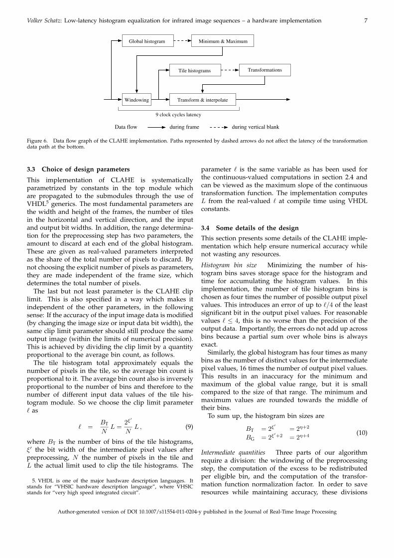
Table 1. Error introduced by neglecting the secondary excess infigure 2 (c) for a Gaussian PDF.

σ ` D

0.05 4 0.0010.05 3 0.003

0.1 3 5.7 · 10−4

0.1 2 0.006

by the constant

S =E(`)

1− 2x0(`)(6)

The quantity we want to compute is the fraction of thehistogram that we ignore by discarding the secondaryexcess after redistribution. Because our PDF is normal-ized, this is equal to the integral of the PDF over thediscarded regions. These are the regions above the cliplimit between the intersection of the shifted PDF with thelimit and the old intersection, as indicated in figure 2 (c).The new intersection points are the same as the points atwhich the original PDF intersects the limit `− S. Theyare therefore given by (4) with ` replaced by `− S. Sothe amount neglected by the single-step redistributionprocedure is

D = 2

∫ x0(`−S)

x0(`)

(p(x+ 1

2 )− (`− S))

dx

=erf√

log(N/(`− S))− erf√

log(N/`)

erf((

2√

2σ)−1) (7)

− 2σ(√

log(N/(`− S))−√

log(N/`))

(`− S)

Some values of D for typical parameter values aredisplayed in table 1. ` is necessarily larger than 1,since that is the average of the normalized PDF. On theother hand, if ` is chosen much larger than 1, it exceedsthe height of the PDF peak, and no clipping happens.Table 1 shows cases with a reasonable value of ` wherethe peak is high enough (σ is small enough) that clippingoccurs. As the table shows, the secondary excess is lessthan one percent of the total in all cases.

In addition to the above general derivation, the single-step redistribution procedure was tested on real-lifeimages. The images were IR images available at theauthor’s institute as well as standard test image seriesfrom the Signal and Image Processing Institute of theUniversity of Southern California1 and imagecompres-sion.info2. The latter is available in a bit depth of 16bits. The colour images from USC-SIPI were convertedto greyscale before processing. Five images from theUSC-SIPI Miscellaneous series and one image from im-agecompression.info were left out because they do notdepict natural scenes. The results are shown in table 2.They have the same order of magnitude as the results

1. http://sipi.usc.edu/database/index.html2. http://www.imagecompression.info/test images/


http://sipi.usc.edu/database/index.html

http://www.imagecompression.info/test_images/

http://dx.doi.org/10.1007/s11554-011-0204-y


Table 2. Error introduced by neglecting the secondary excess in figure 2 (c), averaged over various test image series.Source Series Bit depth Number of images D (` = 3) D (` = 4)

This author IR 14 11 0.0017 8.7 · 10−4

imagecompression.info Gray 16 bit 16 14 9.5 · 10−4 5.7 · 10−4

USC-SIPI Aerials 8 38 0.001 2.6 · 10−4

USC-SIPI Miscellaneous 8 39 0.001 4.2 · 10−4

of the formal calculation and are consistently better for` = 4.

2.5 PreprocessingIn this implementation, the actual histogram equaliza-tion is preceded by a preprocessing step. This is com-mendable due to some characteristics of the IR imagesthat are to be processed. Because of the challengesinvolved in manufacturing IR imaging sensors, suchsensors are not perfect but contain a significant numberof bad pixels which always have the minimum or max-imum grey value. Also, in most situations the occupiedrange of grey values is smaller than the maximumdynamic range. Both effects can be seen in the examplehistogram in figure 3. These effects would reduce the dy-namic range of the result image if histogram equalizationwere performed immediately. In attempting to stretchthe bad pixels accumulated at either end of the inputdynamic range, CLAHE would create a gap next to theminimum or maximum value. In addition, the contrastlimiting would prevent the empty regions between theminimum or maximum and the occupied range frombeing squashed, causing the corresponding region of theoutput range to be wasted.

Both these problems are solved by applying a win-dowing transformation to the grey values before per-forming histogram equalization: Based on the globalhistogram of the image, a certain share of the largestand smallest values are discarded as bad pixels. Theremaining pixels are scaled linearly to occupy the fullrange of an intermediate value, which is then input intothe CLAHE step. The share of pixels to discard is acharacteristic of the camera, which has to be determinedmanually.

3 IMPLEMENTATION

3.1 GeneralThis and the following sections will concentrate on newaspects of the implementation and describe its structurevery briefly. Readers aiming to reproduce the implemen-tation should refer to the appendix and to the descriptionof the hardware implementation in [Rez04].

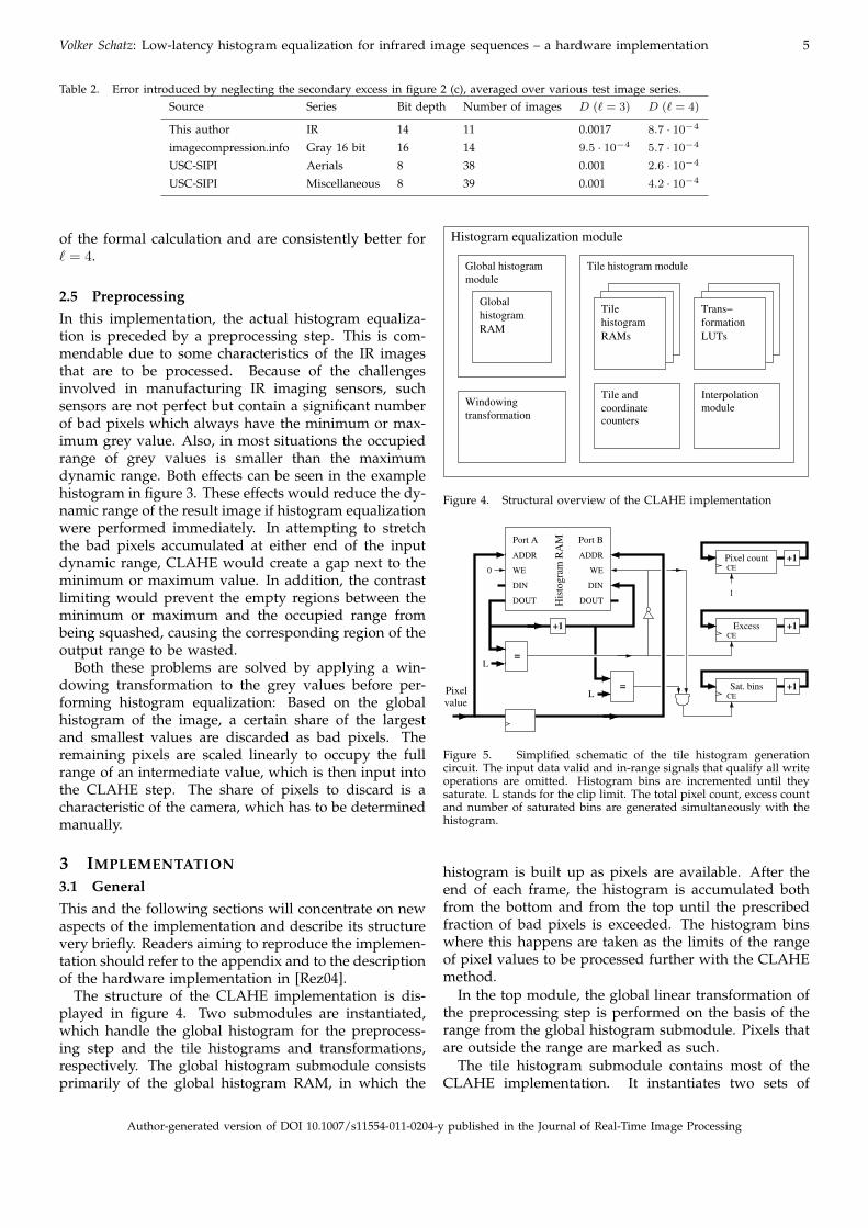
The structure of the CLAHE implementation is dis-played in figure 4. Two submodules are instantiated,which handle the global histogram for the preprocess-ing step and the tile histograms and transformations,respectively. The global histogram submodule consistsprimarily of the global histogram RAM, in which the

Histogram equalization module

Tile histogram moduleGlobal histogram

module

Windowing

transformation

Interpolation

histogram formation

RAMs LUTs

module

counterscoordinate

Tile and

Trans−Tilehistogram

RAM

Global

Figure 4. Structural overview of the CLAHE implementation

Port A

=

=

DOUT

DIN

ADDRADDR

WE

DIN

DOUT

Port B

WE

value

Pixel

His

togra

m R

AM

1

0

L

L

+1

CE

CE

+1

+1

+1

Pixel count

Sat. bins

CE

Excess

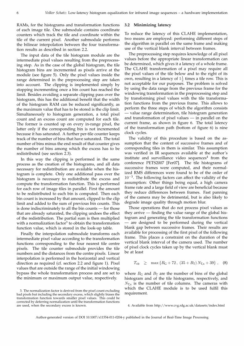
Figure 5. Simplified schematic of the tile histogram generationcircuit. The input data valid and in-range signals that qualify all writeoperations are omitted. Histogram bins are incremented until theysaturate. L stands for the clip limit. The total pixel count, excess countand number of saturated bins are generated simultaneously with thehistogram.

histogram is built up as pixels are available. After theend of each frame, the histogram is accumulated bothfrom the bottom and from the top until the prescribedfraction of bad pixels is exceeded. The histogram binswhere this happens are taken as the limits of the rangeof pixel values to be processed further with the CLAHEmethod.

In the top module, the global linear transformation ofthe preprocessing step is performed on the basis of therange from the global histogram submodule. Pixels thatare outside the range are marked as such.

The tile histogram submodule contains most of theCLAHE implementation. It instantiates two sets of


http://dx.doi.org/10.1007/s11554-011-0204-y


RAMs, for the histograms and transformation functionsof each image tile. One submodule contains coordinatecounters which track the tile and coordinate within thetile of the current pixel. Another submodule performsthe bilinear interpolation between the four transforma-tion results as described in section 2.2.

The input data of the tile histogram module are theintermediate pixel values resulting from the preprocess-ing step. As in the case of the global histogram, the tilehistogram bins are incremented as pixels arrive at themodule (see figure 5). Only the pixel values inside therange determined in the preprocessing step are takeninto account. The clipping is implemented simply bystopping incrementing once a bin count has reached thelimit. Besides avoiding a separate clipping pass over thehistogram, this has the additional benefit that the widthof the histogram RAM can be reduced significantly, asthe maximum value that has to be stored is the clip limit.Simultaneously to histogram generation, a total pixelcount and an excess count are computed for each tile.The former is counted up on every in-range pixel, thelatter only if the corresponding bin is not incrementedbecause it has saturated. A further per-tile counter keepstrack of the number of bins that have saturated. The totalnumber of bins minus the end result of that counter givesthe number of bins among which the excess has to beredistributed (see section 2.3).

In this way the clipping is performed in the sameprocess as the creation of the histograms, and all datanecessary for redistribution are available when the his-togram is complete. Only one additional pass over thehistogram is necessary to redistribute the excess andcompute the transformation function. This is performedfor each row of image tiles in parallel. First the amountto be redistributed to each bin is computed. Then eachbin count is increased by that amount, clipped to the cliplimit and added to the sum of previous bin counts. Thisis done indiscriminately to all the bin counts — for thosethat are already saturated, the clipping undoes the effectof the redistribution. The partial sum is then multipliedwith a normalization factor3 to obtain the transformationfunction value, which is stored in the look-up table.

Finally the interpolation submodule transforms eachintermediate pixel value according to the transformationfunctions corresponding to the four nearest tile centrepixels. The tile counter submodule provides the tilenumbers and the distances from the centre pixels. Linearinterpolation is performed in the horizontal and verticaldirection as required (cf. section 2.2 and figure 1). Pixelvalues that are outside the range of the initial windowingbypass the whole transformation process and are set tothe minimum or maximum output value, respectively.

3. The normalization factor is derived from the pixel count excludingbad pixels but including the secondary excess, which slightly biases thetransformation function towards smaller pixel values. This could becorrected by deferring normalization until the transformation functionsare used, when the secondary excess is known.

3.2 Minimizing latency

To reduce the latency of this CLAHE implementation,two means are employed: performing different steps ofthe algorithm in parallel on the same frame and makinguse of the vertical blank interval between frames.

The preprocessing step requires knowledge of all pixelvalues before the appropriate linear transformation canbe determined, which gives it a latency of a whole frame.The CLAHE transformation of a pixel may require allthe pixel values of the tile below and to the right of itsown, resulting in a latency of 1 1

2 times a tile row. This isnot acceptable for our purposes. The problem is solvedby using the data range from the previous frame for thewindowing transformation in the preprocessing step andby transforming pixel values with the tile transforma-tion functions from the previous frame. This allows toperform the three steps of which the algorithm consists— value range determination, tile histogram generationand transformation of pixel values — in parallel on thecurrent frame, as shown in figure 6. The total latencyof the transformation path (bottom of figure 6) is nineclock cycles.

The validity of this procedure is based on the as-sumption that the content of successive frames and ofcorresponding tiles in them is similar. This assumptionwas verified in IR sequences available at the author’sinstitute and surveillance video sequences4 from theconference PETS2007 [Fer07]. The tile histograms ofsuccessive frames were computed, and their normal-ized RMS differences were found to be of the order of10−3. The following factors can affect the validity of theassumption: Other things being equal, a high cameraframe rate and a large field of view are beneficial becausethey reduce differences between frames. Fast panningof the camera may be detrimental, but is also likely todegrade image quality through motion blur.

Those operations that do not process pixel values asthey arrive — finding the value range of the global his-togram and generating the tile transformation functions— are designed to be performed during the verticalblank gap between successive frames. Their results areavailable for processing of the first pixel of the followingframe. This places a constraint on the duration of thevertical blank interval of the camera used. The numberof pixel clock cycles taken up by the vertical blank mustbe at least

Tvb ≥ max {BG + 72 , (35 +BT)NT,x + 39} , (8)

where BG and BT are the number of bins of the globalhistogram and of the tile histograms, respectively, andNT,x is the number of tile columns. The cameras withwhich the CLAHE module is to be used fulfil thisrequirement.

4. Available from http://www.cvg.rdg.ac.uk/datasets/index.html


http://www.cvg.rdg.ac.uk/datasets/index.html

http://dx.doi.org/10.1007/s11554-011-0204-y


Global histogram Minimum & Maximum

Tile histograms Transformations

Transform & interpolate

Data flow during vertical blankduring frame

9 clock cycles latency

Windowing

Figure 6. Data flow graph of the CLAHE implementation. Paths represented by dashed arrows do not affect the latency of the transformationdata path at the bottom.

3.3 Choice of design parameters

This implementation of CLAHE is systematicallyparametrized by constants in the top module whichare propagated to the submodules through the use ofVHDL5 generics. The most fundamental parameters arethe width and height of the frames, the number of tilesin the horizontal and vertical direction, and the inputand output bit widths. In addition, the range determina-tion for the preprocessing step has two parameters, theamount to discard at each end of the global histogram.These are given as real-valued parameters interpretedas the share of the total number of pixels to discard. Bynot choosing the explicit number of pixels as parameters,they are made independent of the frame size, whichdetermines the total number of pixels.

The last but not least parameter is the CLAHE cliplimit. This is also specified in a way which makes itindependent of the other parameters, in the followingsense: If the accuracy of the input image data is modified(by changing the image size or input data bit width), thesame clip limit parameter should still produce the sameoutput image (within the limits of numerical precision).This is achieved by dividing the clip limit by a quantityproportional to the average bin count, as follows.

The tile histogram total approximately equals thenumber of pixels in the tile, so the average bin count isproportional to it. The average bin count also is inverselyproportional to the number of bins and therefore to thenumber of different input data values of the tile his-togram module. So we choose the clip limit parameter` as

` =BT

NL =

2ξ′

NL , (9)

where BT is the number of bins of the tile histograms,ξ′ the bit width of the intermediate pixel values afterpreprocessing, N the number of pixels in the tile andL the actual limit used to clip the tile histograms. The

5. VHDL is one of the major hardware description languages. Itstands for “VHSIC hardware description language”, where VHSICstands for “very high speed integrated circuit”.

parameter ` is the same variable as has been used forthe continuous-valued computations in section 2.4 andcan be viewed as the maximum slope of the continuoustransformation function. The implementation computesL from the real-valued ` at compile time using VHDLconstants.

3.4 Some details of the design

This section presents some details of the CLAHE imple-mentation which help ensure numerical accuracy whilenot wasting any resources.

Histogram bin size Minimizing the number of his-togram bins saves storage space for the histogram andtime for accumulating the histogram values. In thisimplementation, the number of tile histogram bins ischosen as four times the number of possible output pixelvalues. This introduces an error of up to `/4 of the leastsignificant bit in the output pixel values. For reasonablevalues ` ≤ 4, this is no worse than the precision of theoutput data. Importantly, the errors do not add up acrossbins because a partial sum over whole bins is alwaysexact.

Similarly, the global histogram has four times as manybins as the number of distinct values for the intermediatepixel values, 16 times the number of output pixel values.This results in an inaccuracy for the minimum andmaximum of the global value range, but it is smallcompared to the size of that range. The minimum andmaximum values are rounded towards the middle oftheir bins.

To sum up, the histogram bin sizes are

BT = 2ξ′

= 2η+2

BG = 2ξ′+2 = 2η+4 (10)

Intermediate quantities Three parts of our algorithmrequire a division: the windowing of the preprocessingstep, the computation of the excess to be redistributedper eligible bin, and the computation of the transfor-mation function normalization factor. In order to saveresources while maintaining accuracy, these divisions


http://dx.doi.org/10.1007/s11554-011-0204-y


were replaced by multiplications with the inverse of thedenominator, which is computed only once during thevertical blank gap. So as not to introduce numericalerrors, the bit widths of these inverses and other inter-mediate quantities are computed at compile time. This isdone by value range propagation based on the bit widthsof the histogram inputs and the output data.

Exploiting dual-port RAMs Most of today’s FPGA archi-tectures offer dual-port on-chip RAM blocks. Their mostimportant application in this CLAHE implementationis in generating the histograms at a throughput of onepixel per cycle, as displayed in figure 5. One port isused for reading the current bin count, the other forwriting the new count after incrementing. Writing thenew count and reading the (usually different) next binto be incremented is done simultaneously. The existenceof two RAM ports also allows to save storage space bypacking all tile histograms of one tile row into one setof RAM blocks. Every two of the four transformationresults needed for interpolation come from two ports ofthe same RAM.

3.5 Resource usageThe histogram equalization module was synthesized,placed and routed for five different FPGA architectures,the Virtex-II Pro, Virtex-4, Virtex-5, Spartan3 and Spar-tan6, all made by Xilinx. The three Virtex chips aremembers of the high-end FPGA series from Xilinx thatare in use at the author’s institute. The Virtex-II Proin particular was used for testing and demonstratingthe histogram equalization module (see next section).The Spartan6 and Spartan3 are the newest and previousgenerations of Xilinx low-cost FPGAs.

To determine its resource requirements, the modulealone was synthesized without any logic interfacing acamera or data sink. The synthesis software used wasXilinx ISE. The effort level of the mapper and placerand router was set to “high”. The clock frequencywas slightly overconstrained to determine the maximumfrequency that could be achieved.

Table 3 shows the resource usage and maximum clockfrequency of the histogram equalization module on thefive architectures. Its parameters were a frame size of640 by 480 pixels (VGA resolution), an input bit widthof 14 bits and output bit width of 8 bits, a clip limitof 4, and 8 by 8 tiles. The module fits comfortably onthe large Virtex chips, which makes using it as part ofa larger image processing chain on an FPGA feasible.The two Spartan devices in table 3 are the smallestof their series on which the module fits. The limitingelement is the number of RAM blocks required for thehistograms and transformation functions. The Spartan34000 is the second largest Spartan3, but the Spartan6LX45 is medium-sized for its series [Xil09].

That the clock frequencies in table 3 are relativelylow is mainly due to multiplication operations on num-bers that are wider than the built-in multipliers of the

architecture. In addition, the critical paths sometimescontain multiplexers or adders or subtractors. If clockfrequency was a concern, additional pipeline stagescould be added. However, the pixel clock frequencies ofthe cameras currently used together with the histogramequalization module range from 9 to 16 MHz, so the fre-quencies achieved are quite sufficient. Also, the deviceschosen for the comparison in table 3 are not the fastestspeed grades of their respective series.

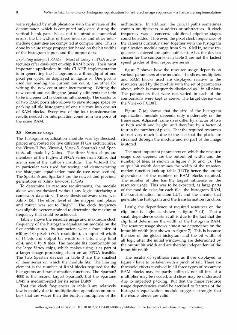
figure 7 shows how the resource usage depends onvarious parameters of the module. The slices, multipliersand RAM blocks used are displayed relative to theresources used by the module with the set of parametersabove, which is consequently displayed as 1 in all plots.The parameters that were not varied in each of thecomparisons were kept as above. The target device wasthe Virtex-5 FX130T.

Figure 7 (a) shows that the size of the histogramequalization module depends only moderately on theframe size. Adjacent frame sizes differ by a factor of twoin both width and height, and therefore by a factor offour in the number of pixels. That the required resourcesdo not vary much is due to the fact that the pixels arestreamed through the module and no part of the imageis stored.

The most important parameters on which the resourceusage does depend are the output bit width and thenumber of tiles, as shown in figure 7 (b) and (c). Theoutput bit width determines the width of the transfor-mation function look-up table (LUT); hence the strongdependence of the number of RAM blocks required.The number of tiles has the largest influence on theresource usage. This was to be expected, as large partsof the module exist for each tile: the histogram RAM,the transformation function LUT, and the circuits thatgenerate the histogram and the transformation function.

Lastly, the dependence of required resources on theclip limit is slight, as shown in figure 7 (d). That asmall dependence exists at all is due to the fact that theclip limit determines the width of the histogram RAM.The resource usage shows almost no dependence on theinput bit width (not shown in figure 7). This is becausethe size of the global histogram and the bit width ofall logic after the initial windowing are determined bythe output bit width and are thereby independent of theinput bit width.

The results of synthesis runs as those displayed infigure 7 have to be taken with a pinch of salt. There arethreshold effects involved in all three types of resources:RAM blocks may be partly utilized, not all bits of amultiplier may be needed, and slices may be underuseddue to imperfect packing. But that the major resourceusage dependencies could be ascribed to features of thehistogram equalization module suggests strongly thatthe results above are valid.


http://dx.doi.org/10.1007/s11554-011-0204-y


Table 3. Resource usage for the fully placed and routed histogram equalization module, not including any interfacing or auxiliary logic. Theparameters of the module are a frame size of 640 by 480 pixels, 14 bits input data width, and 8 by 8 tiles. The small table on the right is toremind the reader that the multipliers and RAM blocks of the Virtex-5 architecture and the slices of the Virtex-5 and Spartan-6 are larger thanthose of the others.

Device Virtex-II Pro Virtex-4 Virtex-5 Spartan-3 Spartan-6Part number xc2vp100-6 xc4vfx100-10 xc5vfx130t-1 xc3s4000-4 xc6slx45-2

Slices 9045 20% 9037 21% 3691 18% 9130 35% 3396 49%Multipliers 27 6% 27 16% 18 5% 27 28% 27 46%RAM blocks 61 13% 61 16% 32 10% 61 63% 61 52%Max. frequency 72.9 MHz 71.8 MHz 101.3 MHz 38.4 MHz 44.7 MHz

Odd-one-out resource sizes

Virtex-5 + Spartan-6 othersLUTs / slice 4× 6 bit 2× 4 bit

Virtex-5 othersMult. width 18× 25 18× 18

BRAM size 36 kb 18 kb

0.5

1

1.5

2

320x240 640x480 1280x960

Resources by frame size

Slices

Multipliers

RAM blocks

(a)

0.5

1

1.5

2

6 7 8 9

Resources by output bit width

Slices

Multipliers

RAM blocks

(b)

0.5

1

1.5

2

4x4 6x6 8x8 10x10

Resources by number of tiles

Slices

Multipliers

RAM blocks

(c)

0.5

1

1.5

2

2 3 4 5

Resources by clip limit

Slices

Multipliers

RAM blocks

(d)Figure 7. Dependence of the resource usage of the histogram equalization module on the frame size, the output bit width, the number of tiles,and the normalized clip limit `. The plots show the number of slices, multipliers and RAM blocks relative to the resources used for a framesize of 640 by 480 pixels, 8 bit output data, 8 by 8 tiles, and clip limit 4. The input data bit width was always 14 bits. The y axes in all plotsare scaled equally for easy comparison. This comparison was performed for the Virtex-5 FX130T.

3.6 Comparison with prior work

There exist two previous hardware implementations ofthe tile-based CLAHE algorithm, by Reza [Rez04] andFerguson et al. [FAEP08]. Reza’s work is aimed at thereal-time visualization of medical X-ray images. He iscareful to keep the latency of his design within thebounds required for that application and achieves alatency of half a frame interval, typically 1/60 of asecond [Rez04]. As the implementation presented in thiswork in addition envisages use in feedback loops suchas object tracking, it was designed to have a latencythat is much lower still, of the order of microseconds.It is therefore completely transparent to downstreamprocessing with respect to latency, not just to the humaneye.

Ferguson et al. have developed a CLAHE implementa-tion for video streams with a bit depth of 8 bits per pixel.In order to minimize size and power consumption, theysacrifice quite a bit of accuracy. The tile histograms arelimited to 8 bins, and it is not discussed whether andhow the resulting 8-step transformation function LUTsare interpolated to utilize the 8-bit range of result values.The implementation given above does not trade off sizefor accuracy and therefore can serve as an accuratebaseline. As a consequence it is considerably larger thanthat presented in [FAEP08].

This work improves upon both prior implementa-tions in several ways. The single-step redistributionprocedure presented in section 2.3 is novel and allowsa more efficient hardware implementation by avoidingrecursion. Unlike prior work, this design is extensivelyparametrized, which allows adapting it to different situ-ations without touching the HDL code. In particular, it

can be synthesized to process input data with an arbi-trary bit depth. Finally, the preprocessing step makes theimplementation tolerant of faulty pixels and increasesaccuracy if not all of the input data range is used.

4 TEST SYSTEM

4.1 Overall design

In order to be able to test and demonstrate the CLAHEmodule, it was implemented together with a camerainterface on a Xilinx Virtex-II Pro FPGA. The designconsists of the camera interface, the histogram equaliza-tion module, a FIFO buffering the transformed imagesand a local bus interface. The local bus data transfersare translated to PCI bus transfers by a bridge chipon the FPGA card. The image data are then displayedby a program running on the host PC. The FPGA cardused was an ADM-XP board from the company AlphaData [Alp04].

Because the CLAHE module has a throughput of onepixel per clock cycle, it can run with the same clock asthe camera interface, and buffering the raw camera datais not required. There needs to be only one clock domaintransition in the design, between the camera clock andthe local bus clock.

The histogram equalization parameters in the testsystem were as follows. The image size was 640 by486 pixels, and the input data bit width was 14 bits,as required by the attached camera. The CLAHE cliplimit was chosen as 4, and the output bit width was 8.Eight by eight tiles were used. The preprocessing stepwas configured to discard 1% of the pixels at either endof the global histogram.


http://dx.doi.org/10.1007/s11554-011-0204-y


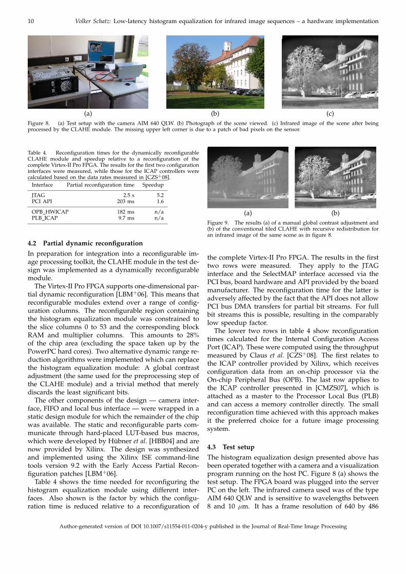
(a) (b) (c)Figure 8. (a) Test setup with the camera AIM 640 QLW. (b) Photograph of the scene viewed. (c) Infrared image of the scene after beingprocessed by the CLAHE module. The missing upper left corner is due to a patch of bad pixels on the sensor.

Table 4. Reconfiguration times for the dynamically reconfigurableCLAHE module and speedup relative to a reconfiguration of thecomplete Virtex-II Pro FPGA. The results for the first two configurationinterfaces were measured, while those for the ICAP controllers werecalculated based on the data rates measured in [CZS+08].

Interface Partial reconfiguration time Speedup

JTAG 2.5 s 5.2PCI API 203 ms 1.6

OPB HWICAP 182 ms n/aPLB ICAP 9.7 ms n/a

4.2 Partial dynamic reconfigurationIn preparation for integration into a reconfigurable im-age processing toolkit, the CLAHE module in the test de-sign was implemented as a dynamically reconfigurablemodule.

The Virtex-II Pro FPGA supports one-dimensional par-tial dynamic reconfiguration [LBM+06]. This means thatreconfigurable modules extend over a range of config-uration columns. The reconfigurable region containingthe histogram equalization module was constrained tothe slice columns 0 to 53 and the corresponding blockRAM and multiplier columns. This amounts to 28%of the chip area (excluding the space taken up by thePowerPC hard cores). Two alternative dynamic range re-duction algorithms were implemented which can replacethe histogram equalization module: A global contrastadjustment (the same used for the preprocessing step ofthe CLAHE module) and a trivial method that merelydiscards the least significant bits.

The other components of the design — camera inter-face, FIFO and local bus interface — were wrapped in astatic design module for which the remainder of the chipwas available. The static and reconfigurable parts com-municate through hard-placed LUT-based bus macros,which were developed by Hubner et al. [HBB04] and arenow provided by Xilinx. The design was synthesizedand implemented using the Xilinx ISE command-linetools version 9.2 with the Early Access Partial Recon-figuration patches [LBM+06].

Table 4 shows the time needed for reconfiguring thehistogram equalization module using different inter-faces. Also shown is the factor by which the configu-ration time is reduced relative to a reconfiguration of

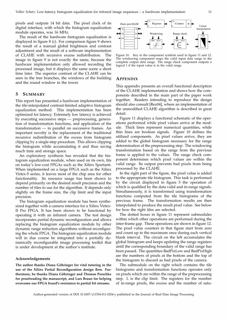
(a) (b)Figure 9. The results (a) of a manual global contrast adjustment and(b) of the conventional tiled CLAHE with recursive redistribution foran infrared image of the same scene as in figure 8.

the complete Virtex-II Pro FPGA. The results in the firsttwo rows were measured. They apply to the JTAGinterface and the SelectMAP interface accessed via thePCI bus, board hardware and API provided by the boardmanufacturer. The reconfiguration time for the latter isadversely affected by the fact that the API does not allowPCI bus DMA transfers for partial bit streams. For fullbit streams this is possible, resulting in the comparablylow speedup factor.

The lower two rows in table 4 show reconfigurationtimes calculated for the Internal Configuration AccessPort (ICAP). These were computed using the throughputmeasured by Claus et al. [CZS+08]. The first relates tothe ICAP controller provided by Xilinx, which receivesconfiguration data from an on-chip processor via theOn-chip Peripheral Bus (OPB). The last row applies tothe ICAP controller presented in [CMZS07], which isattached as a master to the Processor Local Bus (PLB)and can access a memory controller directly. The smallreconfiguration time achieved with this approach makesit the preferred choice for a future image processingsystem.

4.3 Test setupThe histogram equalization design presented above hasbeen operated together with a camera and a visualizationprogram running on the host PC. Figure 8 (a) shows thetest setup. The FPGA board was plugged into the serverPC on the left. The infrared camera used was of the typeAIM 640 QLW and is sensitive to wavelengths between8 and 10 µm. It has a frame resolution of 640 by 486


http://dx.doi.org/10.1007/s11554-011-0204-y


pixels and outputs 14 bit data. The pixel clock of itsdigital interface, with which the histogram equalizationmodule operates, was 16 MHz.

The result of the hardware histogram equalization isdisplayed in figure 8 (c). For comparison figure 9 showsthe result of a manual global brightness and contrastadjustment and the result of a software implementationof CLAHE with recursive excess redistribution. Theimage in figure 9 is not exactly the same, because thehardware implementation only allowed recording theprocessed image, but it displays the same scene a shorttime later. The superior contrast of the CLAHE can beseen in the tree branches, the windows of the buildingand the round window in the tower.

5 SUMMARY

This report has presented a hardware implementation ofthe tile-interpolated contrast-limited adaptive histogramequalization method. This implementation has beenoptimized for latency. Extremely low latency is achievedby executing successive steps — preprocessing, genera-tion of transformation functions, and application of thetransformation — in parallel on successive frames. Animportant novelty is the replacement of the traditionalrecursive redistribution of the excess from histogramclipping by a single-step procedure. This allows clippingthe histogram while accumulating it and thus savingmuch time and storage space.

An exploratory synthesis has revealed that the his-togram equalization module, when used on its own, fitson today’s low-cost FPGAs such as the Xilinx Spartan6.When implemented on a large FPGA such as the XilinxVirtex-5 series, it leaves most of the chip area for otherfunctionality. Its resource usage has been shown todepend primarily on the desired result precision and thenumber of tiles to use for the algorithm. It depends onlyslightly on the frame size, the clip limit and the inputprecision.

The histogram equalization module has been synthe-sized together with a camera interface for a Xilinx Virtex-II Pro FPGA. It has been shown to be functional byoperating it with an infrared camera. The test designincorporates partial dynamic reconfiguration and allowsreplacing the histogram equalization module by otherdynamic range reduction algorithms without reconfigur-ing the whole FPGA. The histogram equalization modulewill in due course be integrated into a partially dy-namically reconfigurable image processing toolkit thatis under development at the author’s institute.

Acknowledgements

The author thanks Diana Gohringer for vital tutoring in theuse of the Xilinx Partial Reconfiguration design flow. Fur-thermore, he thanks Diana Gohringer and Thomas Perschkefor proofreading the manuscript, and Lars Braun for helpingovercome our FPGA board’s resistance to partial bit streams.

Dual−port RAM

Range checkWindowing

RegisterCE

+CE

CounterLinear

interpolationA

DD

A

WEWE

MIN MAXMIN MAX

CTRL

Figure 10. Key to the component symbols used in figure 11 and 12.The windowing component maps the valid input data range to thecomplete output data range. The range check component outputs alogical 1 if the input value is in the valid range.

APPENDIX

This appendix presents an overall functional descriptionof the CLAHE implementation and shows how the com-ponents described in the main part of the paper worktogether. Readers intending to reproduce the designshould also consult [Rez04], where an implementation ofthe unmodified CLAHE algorithm is described in greatdetail.

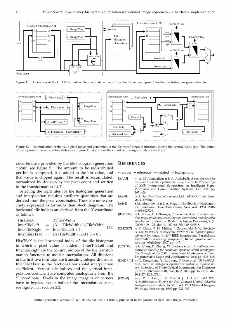
Figure 11 displays a functional schematic of the oper-ations performed while pixel values arrive at the mod-ule. Thick lines represent numerical quantities, whilethin lines are boolean signals. Figure 10 defines theutilized components. As pixel values arrive, they areadded to the global histogram necessary for the rangedetermination of the preprocessing step. The windowingtransformation based on the range from the previousframe is applied to the values. The range check com-ponent determines which pixel values are within thevalid range. Its output prevents bad pixels from beingprocessed by the CLAHE.

In the right part of the figure, the pixel value is addedto the appropriate tile histogram. This task is performedby the circuit displayed in figure 5 the operation ofwhich is qualified by the data valid and in-range signals.Simultaneously, it is transformed using transformationfunctions computed from the tile histograms of theprevious frame. The transformation results are theninterpolated to produce the result pixel value. See belowfor how the right tiles are selected.

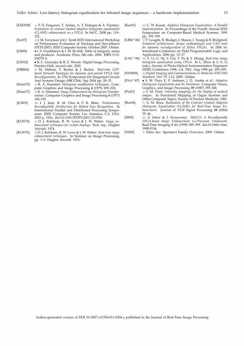
The dotted boxes in figure 11 represent submoduleswithin which other operations are performed during theinter-frame gap. These operations are shown in figure 12.The pixel value counters in that figure start from zeroand count up to the maximum once during each verticalblank interval. The circuit on the left accumulates theglobal histogram and keeps updating the range registersuntil the corresponding boundary of the valid range hasbeen passed. The quantities BadPixLow and BadPixHighare the numbers of pixels at the bottom and the top ofthe histogram to discard as bad pixels of the camera.

The submodule on the right which contains the tilehistograms and transformation functions operates onlyon pixels which are within the range of the preprocessingstep. L is the clip limit. The registers for the numberof in-range pixels, the excess and the number of satu-


http://dx.doi.org/10.1007/s11554-011-0204-y


RangeMin

RangeMax Tile

Generation

Histogram

InterTileXFrac

InterTileYFrac

Transformation LUTsGlobal Histogram RAM

DAV

Pixel value

InterTileXFrac

DAVA

DD

A

WEWE

MIN MAX

MIN MAX

D

A

CTRL

CTRL

1

CTRL

bottom left

bottom right

top

top

left

0

0

0

0

1

1

1

right

+1

Figure 11. Operation of the CLAHE circuit while pixel data arrive during the frame. See figure 5 for the tile histogram generation circuit.

:

:+ Partial sum

< BadPixLow ?

<= FrameSize − BadPixHigh ?

+Pixel value

CE

RangeMin

CE

RangeMax

+Pixel value

Total Bins

Saturated Bins

__ +

L

+

Partial sum

Pixel count

>L?

Global histogram RAM

Excess

Tile histogram RAM

_

Transformation LUT

A

DD

A

WEWE

A

DD

A

WEWE

D

A

0

1

Figure 12. Determination of the valid pixel range and generation of the tile transformation functions during the vertical blank gap. The dottedboxes represent the same submodules as in figure 11. A copy of the circuit on the right exists for each tile.

rated bins are provided by the tile histogram generationcircuit, see figure 5. The amount to be redistributedper bin is computed, it is added to the bin value, andthat value is clipped again. The result is accumulated,normalized by division by the pixel count and writtento the transformation LUT.

Selecting the right tiles for tile histogram generationand interpolation requires auxiliary quantities that arederived from the pixel coordinates. These are more con-cisely expressed as formulas than block diagrams. Thehorizontal tile indices are derived from the X coordinateas follows:HistTileX = X/TileWidthInterTileLeft = (X − TileWidth/2)/TileWidthInterTileRight = InterTileLeft + 1InterTileXFrac = (X/TileWidth) mod 1.0− 0.5

(11)

HistTileX is the horizontal index of the tile histogramto which a pixel value is added. InterTileLeft andInterTileRight are the column indices of the tile transfor-mation functions to use for interpolation. All divisionsin the first two formulas are truncating integer divisions.InterTileXFrac is the fractional horizontal interpolationcoefficient. Vertical tile indices and the vertical inter-polation coefficient are computed analogously from theY coordinate. Pixels in the image margins or cornershave to bypass one or both of the interpolation steps,see figure 1 in section 2.2.

REFERENCES

∼ confer • reference ] related ^ background

[AA05] ] A. M. Alsuwailem & S. A. Aishebeili: A new approach forreal-time histogram equalization using FPGA. In Proceedingsof 2005 International Symposium on Intelligent SignalProcessing and Communication Systems. Dec 2005 pp.397–400.

[Alp04] ^ Alpha Data Parallel Systems Ltd.: ADM-XP data sheet.2004. Online.

[AS64] • M. Abramowitz & I. A. Stegun: Handbook of Mathemat-ical Functions. Dover Publication, New York. 1964. ISBN0-486-61272-4.

[BGP+09] ^ L. Braun, D. Gohringer, T. Perschke et al.: Adaptive real-time image processing exploiting two dimensional reconfigurablearchitecture. Journal of Real-Time Image Processing 4 (2)(2009) 109–125. doi:10.1007/s11554-008-0095-8.

[CMZS07] ^ C. Claus, F. H. Muller, J. Zeppenfeld & W. Stechele:A new framework to accelerate Virtex-II Pro dynamic partialself-reconfiguration. In 21st IEEE International Parallel andDistributed Processing Symposium, Reconfigurable Archi-tectures Workshop. 2007 pp. 1–7.

[CZS+08] ^ C. Claus, B. Zhang, W. Stechele et al.: A multi-platformcontroller allowing for maximum dynamic partial reconfigura-tion throughput. In 2008 International Conference on FieldProgrammable Logic and Applications. 2008 pp. 535–538.

[DND+01] ] G. Dongsheng, Y. Nansheng, P. Defu et al.: DSP+FPGA-based real-time histogram equalization system of infrared im-age. In Society of Photo-Optical Instrumentation Engineers(SPIE) Conference 2001, vol. 4602. 2001 pp. 160–165. doi:10.1117/12.445721.

[EPA90] ] J. P. Ericksen, S. M. Pizer & J. D. Austin: MAHEM:A Multiprocessor Engine for Fast Contrast-Limited AdaptiveHistogram Equalization. In SPIE Vol. 1233 Medical ImagingIV: Image Processing. 1990 pp. 322–333.


http://www.alpha-data.co.uk/archive/adm-xp.pdf

http://dx.doi.org/10.1007/s11554-011-0204-y


[FAEP08] ∼ P. D. Ferguson, T. Arslan, A. T. Erdogan & A. Parmley:Evaluation of contrast limited adaptive histogram equalization(CLAHE) enhancement on a FPGA. In SoCC. 2008 pp. 119–122.

[Fer07] ^ J. M. Ferryman (ed.): Tenth IEEE International Workshopon Performance Evaluation of Tracking and Surveillance(PETS 2007). IEEE Computer Society. October 2007. Online.

[GR00] • I. S. Gradshteyn & I. M. Ryzhik: Table of integrals, seriesand products. Academic Press, 6th edn. 2000. ISBN 0-12-294757-6.

[GW02] • R. C. Gonzalez & R. E. Woods: Digital Image Processing.Prentice-Hall, second edn. 2002.

[HBB04] ^ M. Hubner, T. Becker & J. Becker: Real-time LUT-based Network Topologies for dynamic and partial FPGA Self-Reconfiguration. In 17th Symposium On Integrated CircuitsAnd Systems Design (SBCCI04). Sep 2004 pp. 28–32.

[Hum75] ^ R. A. Hummel: Histogram modification techniques. Com-puter Graphics and Image Processing 4 (1975) 209–224.

[Hum77] ^ R. A. Hummel: Image Enhancement by Histogram Transfor-mation. Computer Graphics and Image Processing 6 (1977)184–195.

[JCR03] ] I. J. Jeon, B. M. Choi & P. K. Rhee: EvolutionaryReconfigurable Architecture for Robust Face Recognition. InInternational Parallel and Distributed Processing Sympo-sium. IEEE Computer Society, Los Alamitos, CA, USA.2003 p. 192a. doi:10.1109/IPDPS.2003.1213356.

[KLW74] ^ D. J. Ketcham, R. W. Lowe & J. W. Weber: Image en-hancement techniques for cockpit displays. Tech. rep., HughesAircraft. 1974.

[KLW76] ^ D. J. Ketcham, R. W. Lowe & J. W. Weber: Real-time imageenhancement techniques. In Seminar on Image Processing,pp. 1–6. Hughes Aircraft. 1976.

[Kur91] ] C. W. Kurak: Adaptive Histogram Equalization: A ParallelImplementation. In Proceedings of the Fourth Annual IEEESymposium on Computer-Based Medical Systems. 1991pp. 192–199.

[LBM+06] ^ P. Lysaght, B. Blodget, J. Mason, J. Young & B. Bridgford:Enhanced architectures, design methodologies and CAD toolsfor dynamic reconfiguration of Xilinx FPGAs. In 2006 In-ternational Conference on Field Programmable Logic andApplications. 2006 pp. 12–17.

[LNC+98] ] X. Li, G. Ni, Y. Cui, T. Pu & Y. Zhong: Real-time imagehistogram equalization using FPGA. In L. Zhou & C.-S. Li(eds.), Society of Photo-Optical Instrumentation Engineers(SPIE) Conference 1998, vol. 3561. Aug 1998 pp. 293–299.

[NEM09] ^ Digital Imaging and Communications in Medicine (DICOM)Standard, Part PS 3.14. 2009. Online.

[PAA+87] • S. M. Pizer, E. P. Amburn, J. D. Austin et al.: AdaptiveHistogram Equalization and Its Variations. Computer Vision,Graphics, and Image Processing 39 (1987) 355–368.

[Piz81] ^ S. M. Pizer: Intensity mappings for the display of medicalimages. In Functional Mapping of Organ Systems andOther Computer Topics. Society of Nuclear Medicine. 1981.

[Rez04] ∼ A. M. Reza: Realization of the Contrast Limited AdaptiveHistogram Equalization (CLAHE) for Real-Time Image En-hancement. Journal of VLSI Signal Processing 38 (2004)35–44.

[SS99] ] Z. Salcic & J. Sivaswamy: IMECO: A ReconfigurableFPGA-based Image Enhancement Co-Processor Framework.Real-Time Imaging 5 (6) (1999) 385–395. doi:10.1006/rtim.1998.0134.

[Xil09] ^ Xilinx Inc.: Spartan-6 Family Overview. 2009. Online.


http://www.cvg.rdg.ac.uk/PETS2007/

ftp://medical.nema.org/medical/dicom/2009/09_14pu.pdf

http://www.xilinx.com/support/documentation/data_sheets/ds160.pdf

http://dx.doi.org/10.1007/s11554-011-0204-y

Low-latency histogram equalization for infrared image … · 2011-06-26 · Low-latency histogram...

Documents

Transcript of Low-latency histogram equalization for infrared image … · 2011-06-26 · Low-latency histogram...