Color image histogram equalization by absolute...

www.elsevier.com/locate/cviu

Computer Vision and Image Understanding 107 (2007) 108–122

Color image histogram equalization by absolute discounting back-off

Nikoletta Bassiou, Constantine Kotropoulos *

Department of Informatics, Aristotle University of Thessaloniki, Box 451, Thessaloniki 541 24, Greece

Received 19 April 2006; accepted 13 November 2006Available online 20 January 2007

Communicated by Rastislav Lukac

Abstract

A novel color image histogram equalization approach is proposed that exploits the correlation between color components and it isenhanced by a multi-level smoothing technique borrowed from statistical language engineering. Multi-level smoothing aims at dealingefficiently with the problem of unseen color values, either considered independently or in combination with others. It is applied here tothe HSI color space for the probability of intensity and the probability of saturation given the intensity, while the hue is left unchanged.Moreover, the proposed approach is extended by an empirical technique, which is based on a hue preserving non-linear transformation,in order to eliminate the gamut problem. This is the second method proposed in the paper. The equalized images by the two methods arecompared to those produced by other well-known methods. The better quality of the images equalized by the proposed methods is judgedin terms of their visual appeal and objective figures of merit, such as the entropy and the Kullback–Leibler divergence estimates betweenthe resulting color histogram and the multivariate uniform probability density function.� 2007 Elsevier Inc. All rights reserved.

Keywords: Histogram equalization; Probability smoothing; Color spaces; Gamut

1. Introduction

Image enhancement aims at improving images from thehuman visual perspective. Image features such as edges,boundaries, and contrast are sharpened in a way that theirdynamic range is increased without any change in the infor-mation content inherent in the data [1]. For this purpose,several techniques have been developed. Among othersare contrast manipulation, noise reduction, edge crispeningand sharpening, filtering, pseudocoloring, image interpola-tion and magnification [1].

Contrast manipulation techniques can be classified aseither global or adaptive. Global techniques apply a trans-formation to all image pixels, while adaptive techniquesuse an input–output transformation that varies adaptivelywith the local image characteristics. The more common

1077-3142/$ - see front matter � 2007 Elsevier Inc. All rights reserved.

doi:10.1016/j.cviu.2006.11.012

* Corresponding author. Fax: +30 2310 998453.E-mail addresses: [email protected] (N. Bassiou), costas

@aiia.csd.auth.gr (C. Kotropoulos).

global techniques are linear contrast stretch, histogramequalization, and multichannel filtering. The most commonadaptive techniques are adaptive histogram equalization(AHE) and contrast-limited adaptive histogram equaliza-tion (CLAHE) [2,3]. AHE applies varying gray-scale trans-formations locally to every small image region, thusrequiring the determination of the region size. CLAHEimproves the just described technique by limiting the localcontrast-gain. Two drawbacks of the latter method havebeen identified namely the unavoidable enhancement ofnoise in smooth regions and the image-dependent selectionof the contrast-gain limit [4].

This paper is focused on global techniques with empha-sis to color images. More precisely, the notion of unigramand bigram probabilities together with probability smooth-ing, borrowed from statistical language modeling, isapplied to color histogram equalization in order to jointlyequalize the two components of the HSI color space,namely the saturation and the intensity. The histogramequalization approach is partially built on that proposed

mailto:[email protected]



N. Bassiou, C. Kotropoulos / Computer Vision and Image Understanding 107 (2007) 108–122 109

in Pitas and Kiniklis [5], but it is extended with smoothingthe necessary probabilities in order to counteract the effectof unseen color component combinations, which stemsfrom the dimensionality of the color space and the oftenlimited number of colors present in an image. Additionally,a second method is developed in an effort to eliminate thegamut problem by exploiting the transformations proposedin Naik and Murthy [6]. The performance of the proposedmethods is compared to that of the methods proposed byPitas and Kiniklis [5,7] as well as the separate equalizationof each color component. The comparison is conductedusing not only subjective measures (i.e., how visuallyappealing the equalized images are), but also objective fig-ures of merit, such as the entropy and the Kullback–Leiblerdivergence between the resulted color histogram and thecorresponding multivariate uniform probability densityfunction.

The outline of the paper is as follows. In Section 2, thecolor image histogram equalization methods are brieflypresented. In Section 3, the baseline histogram equalizationapproaches and the novel algorithms, proposed in thispaper, are described. Experimental results are demonstrat-ed in Section 4, and finally, conclusions are drawn in Sec-tion 5. A brief description of the RGB and HSI colorspaces is given in Appendix A.

2. Related works

Histogram equalization is the simplest and most com-monly used technique to enhance gray-level images. Itassumes that the pixel gray levels are independent identicallydistributed random variables (rvs) and the image is a real-ization of an ergodic random field. As a consequence, animage is considered to be more informative, when its histo-gram resembles the uniform distribution. From this pointof view, grayscale histogram equalization exploits the the-ory of functions of one rv that suggests using the cumula-tive distribution function (CDF) of pixel intensity in orderto transform the pixel intensity to a uniformly distributedrv. However, due to the discrete nature of digital images,the histogram of the equalized image can be made approx-imately uniform.

Histogram equalization becomes a tedious task whendealing with color images due to the vectorial nature of

Table 1Color histogram equalization techniques in the RGB color space

Reference Description

[7] 3-D histogram specification with the output histogram being u[10] Histogram Explosion: histogram equalization of the one-dimen[12] Histogram Decimation: uniformly scatter the color points over[13] The cells of a mesh, initially deformed to fit the original histog[15] The image histogram is approximated by an isotropic Gaussian

minimization (applicable to any dimensions)[16] Histogram equalization by exploiting the histogram utilization,

given the other two color components, and their average occup[14] Histogram equalization treated as a color transfer problem, by

uniform one

color. Each color pixel is represented by a vector with asmany components as the color components in a proper col-or space (i.e., the three components Red, Green, and Bluein the RGB space). The complexity of the problem lies alsoin the correlation between the color components as well asthe color perception by humans. The methods described inthis paper either review the efforts to alleviate one or boththese problems or revisit them in order to improve theirperformance.

Historically, the first and the most straightforwardextension of histogram equalization to color images is theapplication of gray-scale histogram equalization separatelyto the different color bands of the color image, ignoringinter-component correlation. Some efforts were alsofocused in spreading the histogram along the principalcomponent axes of the original image [8], or spreadingrepeatedly the three two-dimensional histograms [9].

The systematic research efforts that followed gave rise totwo main algorithm classes. The first class comprises algo-rithms that work on the RGB space either using the 3-Dhistogram or an 1-D histogram of the color image. The sec-ond class is formed by algorithms, which operate in non-linear color spaces, such as the HSI (hue, saturation, andintensity) or the C-Y spaces, that are applied to one ortwo color components. The algorithms for each class areoutlined in Tables 1 and 2 and described next.

In the RGB space, the more representative approachesare 3-D histogram equalization, histogram explosion, andhistogram decimation. 3-D histogram equalization proposedby Trahanias and Venetsanopoulos [7], attempts the exten-sion of cumulative histogram to higher dimensions bymeans of a uniform 3-D histogram specification in theRGB color cube. The 3-D CDF of the original image coloris compared to the ideal uniform CDF, as is furtherexplained in Section 3.2.

Histogram explosion, which was initially proposed byMlsna and Rodriguez [10], aims to exploit the full 3-DRGB gamut. The algorithm selects an operating point pref-erably on the diagonal of the RGB cube (i.e. the gray line)in order to prevent hue changes and draws rays that ema-nate from the operating point, pass through the colorpoints present in the image, and proceed up to the RGBcube facets. An 1-D histogram is then constructed alongeach ray by interpolating the 3-D histogram data between

niformsional histograms constructed by interpolating the 3-D histogram datathe full 3-D gamut in an iterative procedure

ram, is linearly mapped to the cells of a uniform meshmixture and is fitted to a uniform distribution via least-squares error

which depends on the cumulative histograms of each color componentancyestimating a transformation that maps a N-dimensional distribution to a

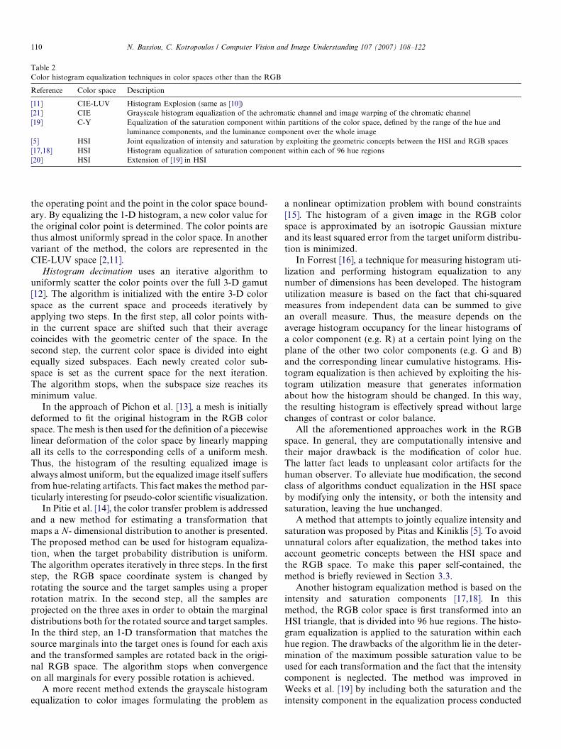
Table 2Color histogram equalization techniques in color spaces other than the RGB

Reference Color space Description

[11] CIE-LUV Histogram Explosion (same as [10])[21] CIE Grayscale histogram equalization of the achromatic channel and image warping of the chromatic channel[19] C-Y Equalization of the saturation component within partitions of the color space, defined by the range of the hue and

luminance components, and the luminance component over the whole image[5] HSI Joint equalization of intensity and saturation by exploiting the geometric concepts between the HSI and RGB spaces[17,18] HSI Histogram equalization of saturation component within each of 96 hue regions[20] HSI Extension of [19] in HSI

110 N. Bassiou, C. Kotropoulos / Computer Vision and Image Understanding 107 (2007) 108–122

the operating point and the point in the color space bound-ary. By equalizing the 1-D histogram, a new color value forthe original color point is determined. The color points arethus almost uniformly spread in the color space. In anothervariant of the method, the colors are represented in theCIE-LUV space [2,11].

Histogram decimation uses an iterative algorithm touniformly scatter the color points over the full 3-D gamut[12]. The algorithm is initialized with the entire 3-D colorspace as the current space and proceeds iteratively byapplying two steps. In the first step, all color points with-in the current space are shifted such that their averagecoincides with the geometric center of the space. In thesecond step, the current color space is divided into eightequally sized subspaces. Each newly created color sub-space is set as the current space for the next iteration.The algorithm stops, when the subspace size reaches itsminimum value.

In the approach of Pichon et al. [13], a mesh is initiallydeformed to fit the original histogram in the RGB colorspace. The mesh is then used for the definition of a piecewiselinear deformation of the color space by linearly mappingall its cells to the corresponding cells of a uniform mesh.Thus, the histogram of the resulting equalized image isalways almost uniform, but the equalized image itself suffersfrom hue-relating artifacts. This fact makes the method par-ticularly interesting for pseudo-color scientific visualization.

In Pitie et al. [14], the color transfer problem is addressedand a new method for estimating a transformation thatmaps a N- dimensional distribution to another is presented.The proposed method can be used for histogram equaliza-tion, when the target probability distribution is uniform.The algorithm operates iteratively in three steps. In the firststep, the RGB space coordinate system is changed byrotating the source and the target samples using a properrotation matrix. In the second step, all the samples areprojected on the three axes in order to obtain the marginaldistributions both for the rotated source and target samples.In the third step, an 1-D transformation that matches thesource marginals into the target ones is found for each axisand the transformed samples are rotated back in the origi-nal RGB space. The algorithm stops when convergenceon all marginals for every possible rotation is achieved.

A more recent method extends the grayscale histogramequalization to color images formulating the problem as

a nonlinear optimization problem with bound constraints[15]. The histogram of a given image in the RGB colorspace is approximated by an isotropic Gaussian mixtureand its least squared error from the target uniform distribu-tion is minimized.

In Forrest [16], a technique for measuring histogram uti-lization and performing histogram equalization to anynumber of dimensions has been developed. The histogramutilization measure is based on the fact that chi-squaredmeasures from independent data can be summed to givean overall measure. Thus, the measure depends on theaverage histogram occupancy for the linear histograms ofa color component (e.g. R) at a certain point lying on theplane of the other two color components (e.g. G and B)and the corresponding linear cumulative histograms. His-togram equalization is then achieved by exploiting the his-togram utilization measure that generates informationabout how the histogram should be changed. In this way,the resulting histogram is effectively spread without largechanges of contrast or color balance.

All the aforementioned approaches work in the RGBspace. In general, they are computationally intensive andtheir major drawback is the modification of color hue.The latter fact leads to unpleasant color artifacts for thehuman observer. To alleviate hue modification, the secondclass of algorithms conduct equalization in the HSI spaceby modifying only the intensity, or both the intensity andsaturation, leaving the hue unchanged.

A method that attempts to jointly equalize intensity andsaturation was proposed by Pitas and Kiniklis [5]. To avoidunnatural colors after equalization, the method takes intoaccount geometric concepts between the HSI space andthe RGB space. To make this paper self-contained, themethod is briefly reviewed in Section 3.3.

Another histogram equalization method is based on theintensity and saturation components [17,18]. In thismethod, the RGB color space is first transformed into anHSI triangle, that is divided into 96 hue regions. The histo-gram equalization is applied to the saturation within eachhue region. The drawbacks of the algorithm lie in the deter-mination of the maximum possible saturation value to beused for each transformation and the fact that the intensitycomponent is neglected. The method was improved inWeeks et al. [19] by including both the saturation and theintensity component in the equalization process conducted


in the color difference (C-Y) space. It was found thatthe transformation yields unrealizable RGB colors in theequalized image. The algorithm partitions the entireC-Y color space, that is transformed into HSI, in n · k

subspaces, where n and k are the number of partitions inhue and intensity components, respectively. Saturation isthen equalized once within the maximum realizable satura-tion of each subspace. Next, the intensity component isequalized by considering the whole image. The methodproposed by Weeks et al. [19] was further applied to theHSI color space by Duan and Qiu [20].

In Luccchese et al. [21], the achromatic channel of acolor image was equalized using a traditional grayscalehistogram equalization method and the chromatic channelwas processed in a way similar to image warping. Thealgorithm works in the xy-chromaticity diagram andconsists of two steps. In the first step, each color pixel istransformed into its maximally saturated value with respectto a certain color gamut. In the second step, the new coloris desaturated toward a new white point.

3. Color histogram equalization methods

3.1. Separate equalization of the three color components—

Method I

This is the most simple approach to color histogramequalization. Since many color images have three colorbases, the color of each pixel is represented by a 3-dimen-sional vector ~X and grayscale histogram equalization isperformed in each of the three color componentsseparately.

Grayscale histogram equalization attempts to uniformlydistribute the pixel gray levels of an image to all theavailable gray levels L (e.g. L = 256, when 8 bits are usedto represent each gray level) [1]. Let us consider the imagepixel gray level to be an rv x. The histogram of a gray scaleimage is the probability density function (PDF) of x

defined as

fxðxkÞ ¼ Pfx ¼ xkg ¼NðxkÞPL�1

m¼0NðxmÞ8 k ¼ 0; 1; . . . ; L� 1;

ð1Þ

where N(xk) is the number of pixels with gray level value xk

[1]. The CDF Fx(xk) of the rv x given by

yk ¼ F xðxkÞ ¼ Pfx 6 xkg ¼Xk

m¼0

f ðxmÞ 8 k ¼ 0; 1; . . . ; L� 1

ð2Þ

defines the transformation function for obtaining the graylevels yk of the equalized image that are uniformly distrib-uted [22].

For color images, the color of each pixel is assumed tobe a random vector ~X ¼ ðxR; xG; xBÞT, where xR, xG, xB

are rvs modeling the Red, Green and Blue components,

respectively. Thus, by applying Eq. (2) the equalizedhistogram of each color component is estimated.

3.2. 3-D Equalization in the RGB space—Method II

The method proposed by Trahanias and Venetsanopou-los [7] is actually a 3-D histogram specification in the RGBcolor space with the output histogram being uniform. Themethod is outlined as follows.

(1) The original 3-D histogram of the color image iscomputed.

(2) The joint CDF is computed both for the originalrandom vector ~X and a random vector ~Y0 ¼ðy0R; y0G; y0BÞ

T that is distributed according to auniform distribution, using Eqs. (3) and (4),respectively,

yRk GsBt¼F xRxGxB

ðxRk ; xGs ; xBt Þ ¼ PfxR 6 xRk ; xG 6 xGs ; xB 6 xBtg

¼Xk

i¼0

Xs

j¼0

Xt

m¼0

f ðxRi ; xGj ; xBmÞ 8 k; s; t ¼ 0; 1; . . . ; L� 1;

ð3Þ

y0Rk0Gs0Bt0¼Xk0

i¼0

Xs0

j¼0

Xt0

m¼0

1

L3

¼ðk0 þ 1Þðs0 þ 1Þðt0 þ 1Þ

L38 k0; s0; t0 ¼ 0;1; . . . ;L� 1;

ð4Þ

where f ðxRi ; xGj ; xBmÞ is the joint PDF.(3) For each color pixel (Rk, Gs, Bt), the smallestðRk0 ;Gs0 ;Bt0 Þ triplet is chosen so that y0Rk0Gs0Bt0

�yRk GsBt

P 0. More precisely, the value of yRk GsBtis

initially compared to the value y0RkGsBt, and in case

yRk GsBtis greater (less) than y0Rk GsBt

, the indices Rk,Gs, Bt are repeatedly increased (decreased), one at atime, until the just mentioned inequality is satisfied.The final triplet values form the color of the equalizedimage.

3.3. Equalization of the intensity component in the HSI space

— Method III

The method in Pitas and Kiniklis [5] studies thegeometrical representation of the HSI space and formu-lates three PDFs for applying histogram equalizationon the intensity component, the saturation component,and jointly the intensity and saturation components.More visually appealing results are obtained, when theintensity component is only used. Saturation used eitherseparately or jointly with intensity admits large values[5].

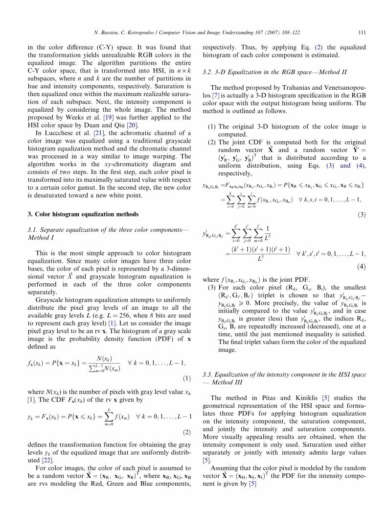
Assuming that the color pixel is modeled by the randomvector ~X ¼ ðxH; xS; xIÞT the PDF for the intensity compo-nent is given by [5]


fxIðxIk Þ ¼

12� x2Ik

for 0 6 xIk 6 0:5

12� ð1� xIk Þ2 for 0:5 6 xIk 6 1:

(ð5Þ

3.4. 2-D Equalization for intensity and saturation in the HSIspace — Method IV

The proposed method works in the HSI color space,where each color pixel is modeled by a random vector~X ¼ ðxH; xS; xIÞT. However, since hue is the most basicattribute of color and changing it results in unacceptablecolor artifacts [5,6,20], the method leaves hue unchangedby considering only the 2-D random vector ~Z ¼ ðx I; xSÞT.Thus, a 2-D histogram should be equalized using the jointCDF F ð~ZÞ ¼ F ðxI; xSÞ ¼ PfxI 6 xI; xS 6 xSg.

Equalization is performed on intensity and saturationsimultaneously by exploiting the following fact [22]:Given n arbitrary rvs xi, the rvs yi formed by

y1 ¼ F ðx1Þ; y2 ¼ F ðx2jx1Þ; . . . ; yn ¼ F ðxnjxn�1; . . . ; x1Þð6Þ

are independent and each is uniform in the interval. (0, 1).Following Eq. (6), the equalized pixel values are

described by a random vector ~Y ¼ ðyI; ySÞT, where yI,yS

are both uniform rvs in (0,1) obtained by the transforma-tions yI = F(zI) and yS = F(zSjzI), respectively,

yIk¼F ðxIk Þ¼ PfxI6 xIkg¼

Xk

m¼0

f ðxImÞ¼Xk

m¼0

P ðxI¼ xImÞ ð7Þ

ySt¼F ðxSt jxIk Þ ¼

Xt

m¼0

f ðxSm jxIk Þ ¼Xt

m¼0

P ðxI ¼ xIk ; xS ¼ xSmÞP ðxI ¼ xIk Þ

:

ð8Þ

In Eqs. (7) and (8), k = 0,1, . . .,L � 1 and t =0,1, . . .,M�1, where L and M are the number of discretelevels for intensity and saturation, respectively. If 8 bitsare used to represent each color component, thenL = M = 256 [23].

Probability smoothingThe method of histogram equalization defined by

Eqs. (7) and (8) suffers from the sparse data problem which

0.2 0.4 0.6 0.8 10

0.2

0.4

0.6

0.8

1

saturation level

prob

abili

ty

0.2 0.40

0.2

0.4

0.6

0.8

1

saturat

prob

abili

ty

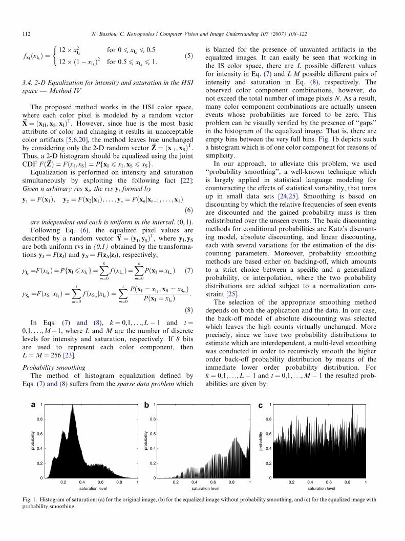
Fig. 1. Histogram of saturation: (a) for the original image, (b) for the equalizedprobability smoothing.

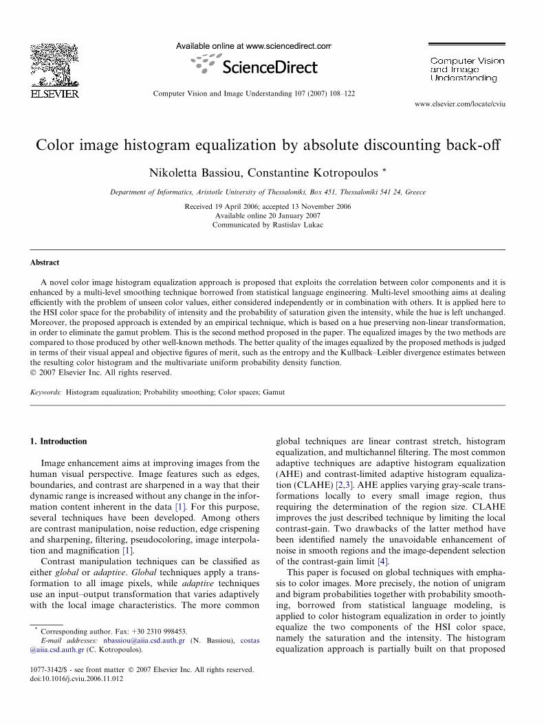
is blamed for the presence of unwanted artifacts in theequalized images. It can easily be seen that working inthe IS color space, there are L possible different valuesfor intensity in Eq. (7) and LÆM possible different pairs ofintensity and saturation in Eq. (8), respectively. Theobserved color component combinations, however, donot exceed the total number of image pixels N. As a result,many color component combinations are actually unseenevents whose probabilities are forced to be zero. Thisproblem can be visually verified by the presence of ‘‘gaps’’in the histogram of the equalized image. That is, there areempty bins between the very full bins. Fig. 1b depicts sucha histogram which is of one color component for reasons ofsimplicity.

In our approach, to alleviate this problem, we used‘‘probability smoothing’’, a well-known technique whichis largely applied in statistical language modeling forcounteracting the effects of statistical variability, that turnsup in small data sets [24,25]. Smoothing is based ondiscounting by which the relative frequencies of seen eventsare discounted and the gained probability mass is thenredistributed over the unseen events. The basic discountingmethods for conditional probabilities are Katz’s discount-ing model, absolute discounting, and linear discounting,each with several variations for the estimation of the dis-counting parameters. Moreover, probability smoothingmethods are based either on backing-off, which amountsto a strict choice between a specific and a generalizedprobability, or interpolation, where the two probabilitydistributions are added subject to a normalization con-straint [25].

The selection of the appropriate smoothing methoddepends on both the application and the data. In our case,the back-off model of absolute discounting was selectedwhich leaves the high counts virtually unchanged. Moreprecisely, since we have two probability distributions toestimate which are interdependent, a multi-level smoothingwas conducted in order to recursively smooth the higherorder back-off probability distribution by means of theimmediate lower order probability distribution. Fork = 0,1, . . .,L � 1 and t = 0,1, . . .,M � 1 the resulted prob-abilities are given by:

0.6 0.8 1

ion level

0.2 0.4 0.6 0.8 10

0.2

0.4

0.6

0.8

1

saturation level

prob

abili

ty

image without probability smoothing, and (c) for the equalized image with

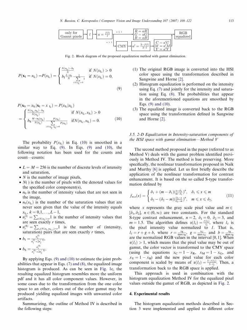
Fig. 2. Block diagram of the proposed equalization method with gamut elimination.


P ðxI ¼ xIk Þ ¼P ðxIk Þ ¼

NðxIkÞ�bI

N if NðxIk Þ > 0

bIL�n0

N1P

i:NðxIiÞ¼0

1if NðxIk Þ ¼ 0;

8><>:

ð9Þ

P ðxS ¼ xSt jxI ¼ x Ik Þ ¼ PðxSt jxIk Þ

¼

NðxIk;xSt Þ�bS

NðxIkÞ if NðxIk ; xStÞ > 0

bSM�n0ðxIk

ÞNðxIk

ÞP ðxSt ÞP

i:NðxIk;xSiÞ¼0

PðxSi ÞifNðxIk ; xStÞ ¼ 0:

8>><>>: ð10Þ

The probability P ðxStÞ in Eq. (10) is smoothed in asimilar way to Eq. (9). In Eqs. (9) and (10), thefollowing notation has been used for the counts andcount—counts:

• L = M = 256 is the number of discrete levels of intensityand saturation,

• N is the number of image pixels,• N(Æ) is the number of pixels with the denoted values for

the specified color component(s),• n0 is the number of intensity values that are not seen in

the image,• n0ðxIk Þ is the number of the saturation values that are

never seen given that the value of the intensity equalsxIk , k = 0,1, . . .,L�1,

• nðIÞr ¼P

i:NðxIi Þ¼r1 is the number of intensity values thatare seen exactly r times,

• nðSÞr ¼P

i;j:NðxIi ;xS¼jÞ¼r1 is the number of (intensity,saturation) pairs that are seen exactly r times,

• bI ¼nðIÞ

1

nðIÞ1þ2nð IÞ

2

,

• bS ¼nðSÞ

1

nðSÞ1þ2nð SÞ

2

.

By applying Eqs. (9) and (10) to estimate the joint prob-abilities that appear in Eqs. (7) and (8), the equalized imagehistogram is produced. As can be seen in Fig. 1c, theresulting equalized histogram resembles more the uniformpdf and it has all color component values. However, insome cases due to the transformation from the one colorspace to an other, colors out of the color gamut may beproduced yielding equalized images with unwanted colorartifacts.

Summarizing, the outline of Method IV is described inthe following steps:

(1) The original RGB image is converted into the HSIcolor space using the transformation described inSangwine and Horne [2].

(2) Histogram equalization is performed on the intensityusing Eq. (7) and jointly for the intensity and satura-tion using Eq. (8). The probabilities that appearin the aforementioned equations are smoothed byEqs. (9) and (10).

(3) The equalized image is converted back to the RGBspace using the transformation defined in Sangwineand Horne [2].

3.5. 2-D Equalization in Intensity-saturation components of

the HSI space with gamut elimination—Method V

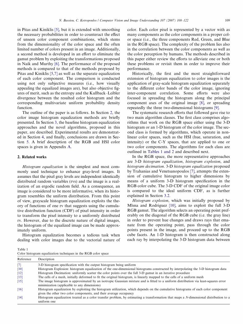
The second method proposed in the paper (referred to asMethod V) deals with the gamut problem identified previ-ously in Method IV. The method is hue preserving. Morespecifically, the nonlinear transformation proposed in Naikand Murthy [6] is applied. Let us first briefly describe theapplication of the nonlinear transformation for contrastenhancement. It is based on the so called S-type transfor-mation defined by

fm;nðxÞ ¼d1 þ ðm� d1Þð x�d1

m�d1Þn; d1 6 x 6 m

d2 � ðd2 � mÞðd2�xd2�m Þ

n; m 6 x 6 d2;

(ð11Þ

where x represents the gray scale pixel value and m 2[d1,d2], n 2 (0,1) are two constants. For the standardS-type contrast enhancement, n = 2, d1 = 0, d2 = 3, andm = 1.5. The algorithm defines aðl~xÞ ¼ f ðl~xÞ

l~x, where l~x is

the pixel intensity value normalized to 1. That is,l~x ¼ r þ g þ b, where r ¼ xR

max xR, g ¼ xG

max xGand b ¼ xB

max xB

are the normalized RGB values in the interval [0,1]. Whenaðl~xÞ > 1, which means that the pixel value may be out ofgamut, the color vector is transformed to the CMY space(using the equations xC = 1 � xR, xM = 1 � xG, andxY = 1 � xB) and the new pixel value for each colorcomponent is scaled by means of aðl~xÞ ¼ 3�f ðl~xÞ

3�l~x. Then, a

transformation back to the RGB space is applied.This approach is used in combination with the

histogram equalization Method IV for the equalized pixelvalues outside the gamut of RGB, as depicted in Fig. 2.

4. Experimental results

The histogram equalization methods described in Sec-tion 3 were implemented and applied to different color


images in order to make a comparative quality assessmentstudy of their performance. The quality of the equalizedimages was judged both in a subjective way from their visu-al appeal and the presence of unwanted color artifacts aswell as by using objective statistical measures, such as theentropy and the Kullback–Leibler divergence.

The entropy represents the average uncertainty of arandom variable and is maximized for the uniformdistribution [24,26]. Therefore it consists a good measuresince greater entropy values show a more uniform distribu-tion. The entropy of a n discrete rvs is defined by

Hðx1; x2; . . . ; xnÞ ¼ �X

x1

Xx2

� � �X

xn

Pðx1; x2; . . . ; xnÞ

� log2P ðx1; x2; . . . ; xnÞ: ð12Þ

In a similar way, the Kullback–Leibler divergence mea-sures the difference between two probability distributions[24,26]. In our experiments, the Kullback–Leibler diver-gence was used in order to measure how similar the histo-grams of the original and the equalized images are to theuniform distribution. The image probabilities which weretaken under consideration were those used for the entropyestimates. That is, for the n-dimensional case

Dðf ðx1; x2; . . . ; xnÞjjgðxu; yu; . . . ; zuÞÞ¼X

x1

Xx2

� � �X

xn

Pðx1; x2; . . . ; xnÞ

� log2

P ðx1; x2; . . . ; xnÞgðx1; x2; . . . ; xnÞ

� �; ð13Þ

where g(x1,x2, . . .,xn) is a n-dimensional uniform distribu-tion defined in the same space with f(x1,x2, . . ., xn).

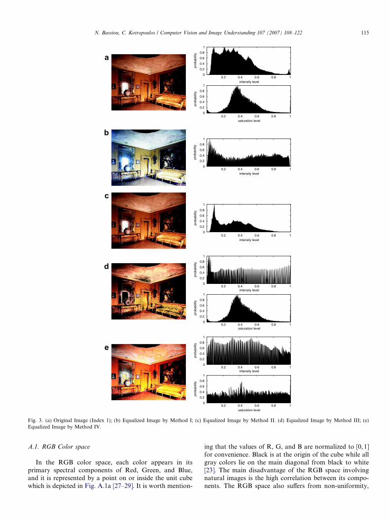
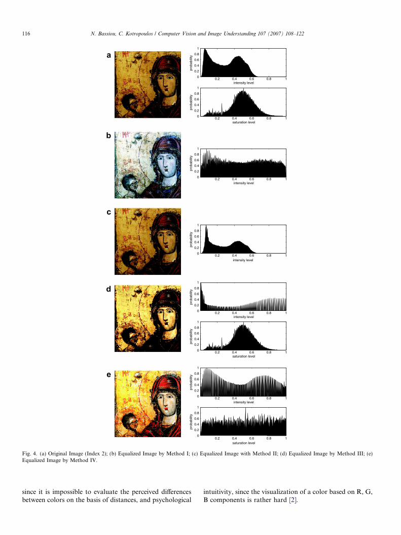
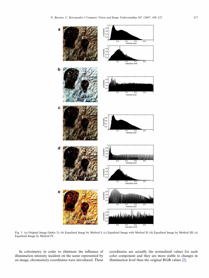
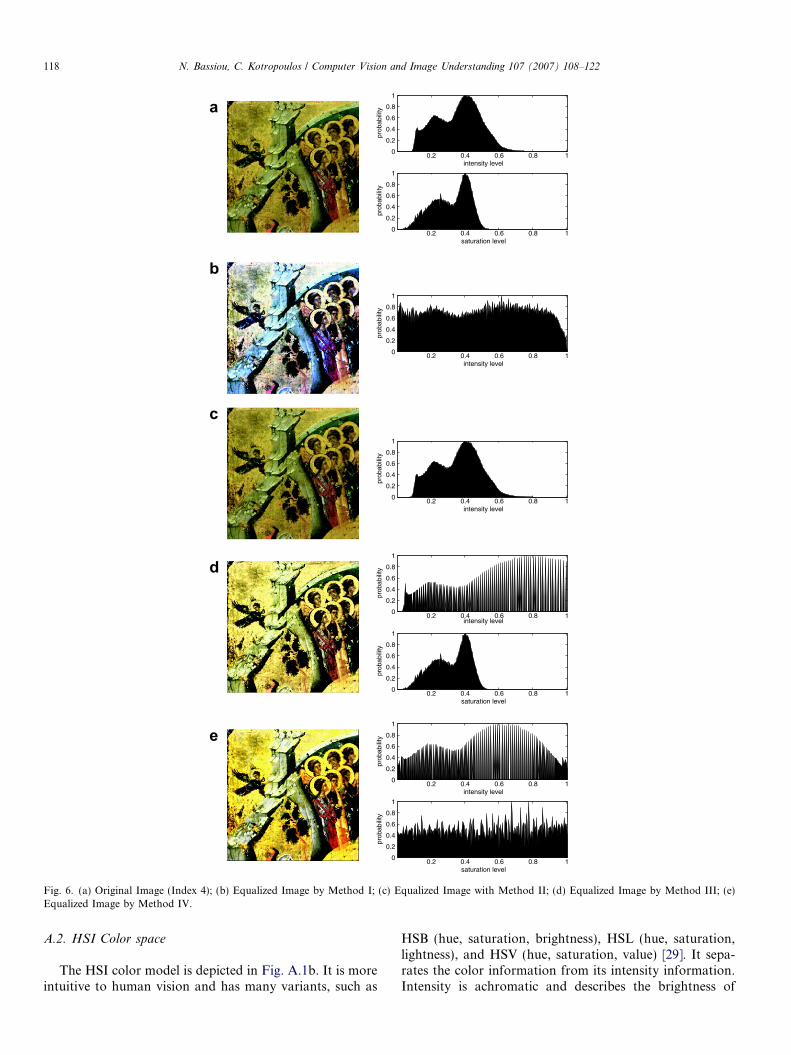
Representative experimental results are presented forfive color images, namely an indoor scene (Index 1) and aset of four digitalized Orthodox Holy Icons (Indices 2–5).The images are depicted in Figs. 3–7 together with their his-tograms for the intensity level for the methods that workon the RGB space (Methods I and II) and the intensityand saturation level for the methods that work on theHSI space (Methods III and IV).

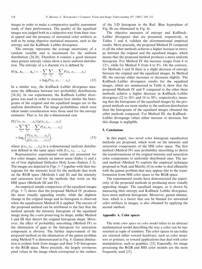
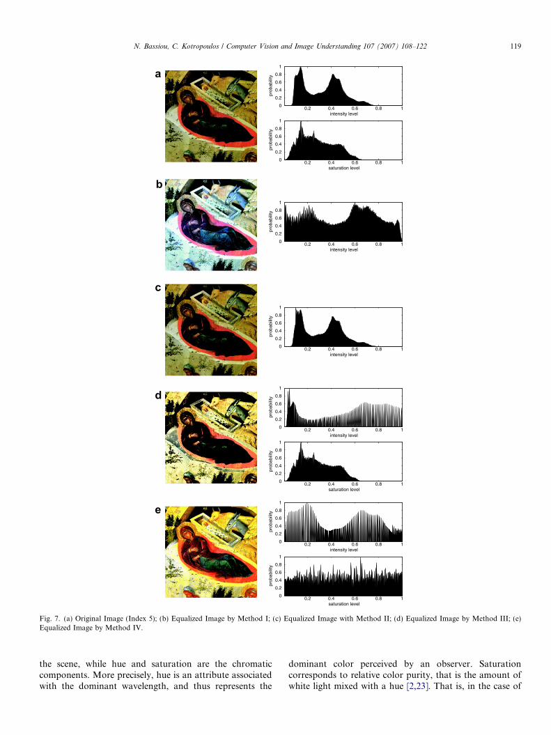
An empirical simple comparison of the equalized images(Figs. 3–7) shows that the proposed Method IV producesthe most visually appealing results, while the slightestchange in the original image and its histogram is observedwhen the equalization Method II is applied. The success ofthe proposed method can be attributed to the fact that themethod spreads the intensity histogram of the equalizedimage along the x-axis preserving its shape, unlike MethodI and III that distort the original histogram shape. More-over, the effect of probability smoothing (Method IV) tothe elimination of gaps in the histogram for saturationcomponent is obvious. The further improvement of theproposed method on the elimination of the gamut problemusing Method V is demonstrated in Fig. 8. Gamut elimina-tion is evident both from images and their 3-D histogramsin the RGB space. More precisely, the largely erroneouspixel values in the image which correspond to the outliers

of the 3-D histogram in the Red. Blue hyperplane ofFig. 8b are eliminated in Fig. 8c.

The objective measures of entropy and Kullback–Leibler divergence that are presented, respectively, inTables 3 and 4, validate the aforementioned empiricalresults. More precisely, the proposed Method IV comparedto all the other methods achieves a higher increase in entro-py between the original and the equalized images, whichmeans that the proposed method produces a more uniformhistogram. For Method IV the increase ranges from 6 to12%, while for Method V from 4 to 8%. On the contrary,for Methods I and II there is a slight decrease of entropybetween the original and the equalized images. In MethodIII, the entropy either increases or decreases slightly. TheKullback–Leibler divergence results for the equalizedimages, which are summarized in Table 4, show that theproposed Methods IV and V compared to the other threemethods achieve a higher decrease in Kullback–Leiblerdivergence (22 to 36% and 16 to 30%, respectively), mean-ing that the histograms of the equalized images by the pro-posed methods are more similar to the uniform distributionthan the histograms of the equalized images obtained theother methods compared. For Method III, the Kullback–Leibler divergenge values either increase or decrease, butthis change is negligible.

5. Conclusions

In this paper, two novel color histogram equalizationmethods are proposed, which work on the intensity andsaturation components of the HSI color space. The firstmethod (Method IV) uses probability smoothing to derivethe transformations of the original intensity and saturationcolor components to uniformly distributed ones. The sec-ond method (Method V) exploits the empirical techniqueproposed in Naik and Murthy [6] in order to deal efficientlywith the gamut problem that may appear due to the trans-formation from HSI color space to the RGB space.

The experimental results have demonstrated the superi-ority of the proposed methods in producing more visuallyappealing images. The equalized images, as is shown bymeasuring their entropy and Kullback–Leibler divergence,have more uniform histograms. Moreover, gamut elimina-tion, which is a factor that can be blamed for unwantedcolor artifacts in images, is also obtained by applying thesecond method.

Appendix A. Color spaces

The term color space or color model refers to an abstractmathematical model describing the way a color can be rep-resented as tuple of numbers. The color spaces in use todayare oriented either toward hardware, such as color moni-tors or printers, or toward applications that deal with colormanipulation, such as graphics. [23]. Especially, for imageprocessing the RGB and HSI color models are the mostfrequently used [23].

a

0.2 0.4 0.6 0.8 10

0.2

0.4

0.6

0.8

1

intensity level

prob

abili

ty

0.2 0.4 0.6 0.8 10

0.2

0.4

0.6

0.8

1

saturation level

prob

abili

ty

b

0.2 0.4 0.6 0.8 10

0.2

0.4

0.6

0.8

1

intensity level

prob

abili

tyc

0.2 0.4 0.6 0.8 10

0.2

0.4

0.6

0.8

1

intensity level

prob

abili

ty

d

0.2 0.4 0.6 0.8 10

0.2

0.4

0.6

0.8

1

intensity level

prob

abili

ty

0.2 0.4 0.6 0.8 10

0.2

0.4

0.6

0.8

1

saturation level

prob

abili

ty

e

0.2 0.4 0.6 0.8 10

0.2

0.4

0.6

0.8

1

intensity level

prob

abili

ty

0.2 0.4 0.6 0.8 10

0.2

0.4

0.6

0.8

1

saturation level

prob

abili

ty

Fig. 3. (a) Original Image (Index 1); (b) Equalized Image by Method I; (c) Equalized Image by Method II. (d) Equalized Image by Method III; (e)Equalized Image by Method IV.


A.1. RGB Color space

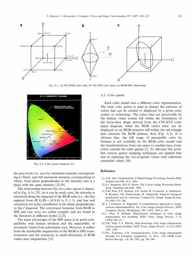
In the RGB color space, each color appears in itsprimary spectral components of Red, Green, and Blue,and it is represented by a point on or inside the unit cubewhich is depicted in Fig. A.1a [27–29]. It is worth mention-

ing that the values of R, G, and B are normalized to [0,1]for convenience. Black is at the origin of the cube while allgray colors lie on the main diagonal from black to white[23]. The main disadvantage of the RGB space involvingnatural images is the high correlation between its compo-nents. The RGB space also suffers from non-uniformity,

a

0.2 0.4 0.6 0.8 10

0.2

0.4

0.6

0.8

1

intensity level

prob

abili

ty

0.2 0.4 0.6 0.8 10

0.2

0.4

0.6

0.8

1

saturation level

prob

abili

ty

b

0.2 0.4 0.6 0.8 10

0.2

0.4

0.6

0.8

1

intensity level

prob

abili

ty

c

0.2 0.4 0.6 0.8 10

0.2

0.4

0.6

0.8

1

intensity level

prob

abili

ty

d

0.2 0.4 0.6 0.8 10

0.2

0.4

0.6

0.8

1

intensity level

prob

abili

ty

0.2 0.4 0.6 0.8 10

0.2

0.4

0.6

0.8

1

saturation level

prob

abili

ty

e

0.2 0.4 0.6 0.8 10

0.2

0.4

0.6

0.8

1

intensity level

prob

abili

ty

0.2 0.4 0.6 0.8 10

0.2

0.4

0.6

0.8

1

saturation level

prob

abili

ty

Fig. 4. (a) Original Image (Index 2); (b) Equalized Image by Method I; (c) Equalized Image with Method II; (d) Equalized Image by Method III; (e)Equalized Image by Method IV.


since it is impossible to evaluate the perceived differencesbetween colors on the basis of distances, and psychological

intuitivity, since the visualization of a color based on R, G,B components is rather hard [2].

a

0.2 0.4 0.6 0.8 10

0.2

0.4

0.6

0.8

1

intensity level

prob

abili

ty

0.2 0.4 0.6 0.8 10

0.2

0.4

0.6

0.8

1

saturation level

prob

abili

ty

b

0.2 0.4 0.6 0.8 10

0.2

0.4

0.6

0.8

1

intensity level

prob

abili

ty

c

0.2 0.4 0.6 0.8 10

0.2

0.4

0.6

0.8

1

intensity level

prob

abili

ty

d

0.2 0.4 0.6 0.8 10

0.2

0.4

0.6

0.8

1

intensity level

prob

abili

ty

0.2 0.4 0.6 0.8 10

0.2

0.4

0.6

0.8

1

saturation level

prob

abili

ty

e

0.2 0.4 0.6 0.8 10

0.2

0.4

0.6

0.8

1

intensity level

prob

abili

ty

0.2 0.4 0.6 0.8 10

0.2

0.4

0.6

0.8

1

saturation level

prob

abili

ty



In colorimetry in order to eliminate the influence ofillumination intensity incident on the scene represented byan image, chromaticity coordinates were introduced. These

coordinates are actually the normalized values for eachcolor component and they are more stable to changes inillumination level than the original RGB values [2].

a

0.2 0.4 0.6 0.8 10

0.2

0.4

0.6

0.8

1

intensity level

prob

abili

ty

0.2 0.4 0.6 0.8 10

0.2

0.4

0.6

0.8

1

saturation level

prob

abili

ty

b

0.2 0.4 0.6 0.8 10

0.2

0.4

0.6

0.8

1

intensity level

prob

abili

ty

c

0.2 0.4 0.6 0.8 10

0.2

0.4

0.6

0.8

1

intensity level

prob

abili

ty

d

0.2 0.4 0.6 0.8 10

0.2

0.4

0.6

0.8

1

intensity level

prob

abili

ty

0.2 0.4 0.6 0.8 10

0.2

0.4

0.6

0.8

1

saturation level

prob

abili

ty

e

0.2 0.4 0.6 0.8 10

0.2

0.4

0.6

0.8

1

intensity level

prob

abili

ty

0.2 0.4 0.6 0.8 10

0.2

0.4

0.6

0.8

1

saturation level

prob

abili

ty



A.2. HSI Color space

The HSI color model is depicted in Fig. A.1b. It is moreintuitive to human vision and has many variants, such as

HSB (hue, saturation, brightness), HSL (hue, saturation,lightness), and HSV (hue, saturation, value) [29]. It sepa-rates the color information from its intensity information.Intensity is achromatic and describes the brightness of

a

0.2 0.4 0.6 0.8 10

0.2

0.4

0.6

0.8

1

intensity level

prob

abili

ty

0.2 0.4 0.6 0.8 10

0.2

0.4

0.6

0.8

1

saturation level

prob

abili

ty

b

0.2 0.4 0.6 0.8 10

0.2

0.4

0.6

0.8

1

intensity level

prob

abili

ty

c

0.2 0.4 0.6 0.8 10

0.2

0.4

0.6

0.8

1

intensity level

prob

abili

ty

d

0.2 0.4 0.6 0.8 10

0.2

0.4

0.6

0.8

1

intensity level

prob

abili

ty

0.2 0.4 0.6 0.8 10

0.2

0.4

0.6

0.8

1

saturation level

prob

abili

ty

e

0.2 0.4 0.6 0.8 10

0.2

0.4

0.6

0.8

1

intensity level

prob

abili

ty

0.2 0.4 0.6 0.8 10

0.2

0.4

0.6

0.8

1

saturation level

prob

abili

ty



the scene, while hue and saturation are the chromaticcomponents. More precisely, hue is an attribute associatedwith the dominant wavelength, and thus represents the

dominant color perceived by an observer. Saturationcorresponds to relative color purity, that is the amount ofwhite light mixed with a hue [2,23]. That is, in the case of

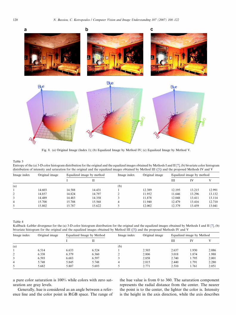
Fig. 8. (a) Original Image (Index 1); (b) Equalized Image by Method IV; (c) Equalized Image by Method V.

Table 3Entropy of the (a) 3-D color histogram distribution for the original and the equalized images obtained by Methods I and II [7], (b) bivariate color histogramdistribution of intensity and saturation for the original and the equalized images obtained by Method III ([5]) and the proposed Methods IV and V

Image index Original image Equalized image by method Image index Original image Equalized image by method

I II III IV V

(a) (b)1 14.603 14.588 14.431 1 12.389 12.195 13.215 12.9912 14.857 14.824 14.797 2 11.952 11.646 13.296 13.1323 14.489 14.483 14.358 3 11.878 12.048 13.411 13.1144 15.708 15.708 15.568 4 11.940 12.479 13.416 12.7105 15.802 15.787 15.622 5 12.002 12.379 13.459 13.041

Table 4Kullback–Leibler divergence for the (a) 3-D color histogram distribution for the original and the equalized images obtained by Methods I and II [7], (b)bivariate histogram for the original and the equalized images obtained by Method III ([5]) and the proposed Methods IV and V

Image index Original image Equalized Image by Method Image index Original image Equalized image by Method

I II III IV V

(a) (b)1 6.514 6.633 6.524 1 2.503 2.637 1.930 2.0862 6.338 6.379 6.360 2 2.806 3.018 1.874 1.9883 6.593 6.683 6.597 3 2.858 2.740 1.795 2.0014 5.748 5.845 5.748 4 2.815 2.440 1.791 2.2805 5.682 5.807 5.693 5 2.771 2.510 1.761 2.051


a pure color saturation is 100% while colors with zero sat-uration are gray levels.

Generally, hue is considered as an angle between a refer-ence line and the color point in RGB space. The range of

the hue value is from 0 to 360. The saturation componentrepresents the radial distance from the center. The nearerthe point is to the center, the lighter the color is. Intensityis the height in the axis direction, while the axis describes

a b c

Fig. A.1. (a) The RGB color cube; (b) The HSI color space; (c) RGB-HSI relationship.

Fig. A.2. Color gamut diagram [23].


the gray levels (i.e. zero for minimum intensity correspond-ing to black, and full maximum intensity corresponding towhite). Each plane perpendicular to the intensity axis is aplane with the same intensity [23,29].

The relationship between the two color spaces is depict-ed in Fig. A.1c [29]. As it can be easily seen, the intensity ismeasured along the diagonal of the RGB cube (i.e., the linesegment from (R,G,B) = (0, 0,0) to (1, 1,1), and hue andsaturation are polar coordinates in the plane perpendicularto the I diagonal. The conversion formulae from RGB toHSI and vice versa are rather complex and are found inthe literature in different forms [2,23].

The main advantages of the HSI space is its good com-patibility with human intuition and the separability ofchromatic values from achromatic ones. However, it suffersfrom the irreducible singularities of the RGB to HSI trans-formation and the sensitivity to small deviations of RGBvalues near singularities [23].

A.3. Color gamut

Each color model uses a different color representation.The term color gamut is used to denote the universe ofcolors that can be created or displayed by a given colorsystem or technology. The colors that are perceivable bythe human visual system fall within the boundaries ofthe horse-shoe shape derived from the CIE-XYZ colorspace diagram, while the RGB colors (that can bedisplayed on an RGB monitor) fall within the red trianglethat connects the RGB primary dots (Fig. A.2). It isobvious that, the full range of perceptible color byhumans is not available by the RGB color model andthe transformations from one space to another may createcolors outside the color gamut [2]. To alleviate this prob-lem various gamut mapping techniques are applied thataim at replacing the out-of-gamut values with substituteattainable values [30].

References

[1] A.K. Jain, Fundamentals of Digital Image Processing, Prentice-Hall,Englewood Cliffs, N.Y, 1986.

[2] S.J. Sangwine, R.E.N. Horne, The Colour Image Processing Hand-book, Chapman and Hall, 1998.

[3] S.M. Pizer, E.P. Amburn, J.D. Austin, R. Cromartie, A. Geselowitz,B. Romeny, J.B. Zimmermann, K. Zuiderveld, Adaptive histogramequalization and its variations, Comput.Vis. Graph. Image Process.39 (1987) 355–368.

[4] A. Carbonaro, P. Zingaretti, A comprehensive approach to image-contrast enhancementProc. Int. Conf. Image Analysis Process., IEEEComputer Society, Washington, DC, USA, 1999, p. 241.

[5] I. Pitas, P. Kiniklis, Multichannel techniques in color imageenhancement and modeling, IEEE Trans. Image Process. 5 (1)(1996) 168–171.

[6] S.K. Naik, C.A. Murthy, Hue-preserving color image enhancementwithout gamut problem, IEEE Trans. Image Process. 12 (12) (2003)1591–1598.

[7] P.E. Trahanias, A.N. Venetsanopoulos, Color image enhancementthrough 3-d histogram equalization, in: Proc. 11th IAPR Conf.Pattern Recogn., vol. III, 1992, pp. 545–548.


[8] J.M. Soha, A.A. Schwartz, Multidimensional histogram normaliza-tion contrast enhancement, in: Proc. 5th Canadian Symp. RemoteSensing, 1978, pp. 86–93.

[9] R.N. Niblack, An Introduction to Digital Image Processing, Prentice-Hall, 1986.

[10] P.A. Mlsna, J.J. Rodriguez, A multivariate contrast enhancementtechnique for multispectral images, IEEE Trans. Geosci. RemoteSensing 33 (1) (1995) 212–216.

[11] P.A. Mlsna, Q. Zhang, J.J. Rodriguez, 3-d histogram modification ofcolor images, in: Proc. IEEE Int. Conf. Image Process., vol. III, 1996,pp. 1015–1018.

[12] Q. Zhang, P.A. Mlsna, J.J. Rodriguez, A recursive technique for 3-dhistogram enhancement of color images, in: Proc. IEEE SouthwestSymp. Image Analysis Interpret., 1996, pp. 218–223.

[13] E. Pichon, M. Niethammer, G. Sapiro, Color histogram equalizationthrough mesh deformation, in: Proc. IEEE Int. Conf. Image Process.,vol. II, 2003, pp. 117–120.

[14] F. Pitie, A.C. Kokaram, R. Dahyot, N-dimensional probabilitydensity function transfer and its application to color transfer, in:Proc. IEEE Int. Conf. Comput. Vis., vol. II, 2005, pp. 1434–1439.

[15] T. Kim, H.S. Yang, Colour histogram equalisation via least-squaresfitting of isotropic gaussian mixture to uniform distribution, IEEElectr. Lett. 42 (8) (2006) 452–454.

[16] A.K. Forrest, Colour histogram equalisation of multichannel images,IEE Proc. Vis. Image Signal Process. 152 (6) (2005) 677–686.

[17] I.M. Bockstein, Color equalization method and its application tocolor image processing, J. Opt. Soc. Am. 3 (5) (1986) 735–737.

[18] W.F. McDonnel, R.N. Strickland, C.S. Kim, Digital color imageenhancement based on the saturation component, Opt. Eng. 26 (7)(1987) 609–616.

[19] A.R. Weeks, G.E. Hague, H.R. Myler, Histogram specification of 24-bit color images in the color difference (C-Y) color space, J. Electron.Imag. 4 (1) (1995) 15–22.

[20] J. Duan, G. Qiu, Novel histogram processing for colour imageenhancement, in: Proc. IEEE Int. Conf. Image Graph., 2004, pp. 55–58.

[21] L. Lucchese, S.K. Mitra, J. Mukherjee, A new algorithm based onsaturation and desaturation in the xy-chromaticity diagram forenhancement and re-rendition of color images, in: Proc. IEEE Int.Conf. Image Process., 2001, pp. 1077–1080.

[22] A. Papoulis, Probability, Random Variables and Stochastic Process-es, 3rd ed., McGraw Hill, New-York, 1991.

[23] R.C. Gonzalez, R.E. Woods, Digital Image Processing, 2nd ed.,Addison Wesley Publishing Company, 1992.

[24] C.D. Manning, H. Schutze, Foundations of Statistical NaturalLanguage Processing, 1st ed., MIT Press, 1999.

[25] H. Ney, S. Martin, F. Wessel, Statistical language modelingusing leaving-one-out, in: S. Young, G. Bloothooft (Eds.),Corpus-Based Methods in Language and Speech Processing,Kluwer Academic Publishers, Dordrecht, The Netherlands, 1997,pp. 174–207.

[26] R.O. Duda, P.E. Hart, D.G. Stork, Pattern Classification, 2nd ed.,Wiley Interscience, N.Y, 2000.

[27] H.R. Kang, Color Technology for Electronic Imaging Devices, SPIEPress, 1997.

[28] K.N. Plataniotis, A.N. Venetsanopoulos, Color Image Processing andApplications, 1st ed., Springer, 2000.

[29] I. Pitas, Digital Image Processing: Algorithms and Applications,J. Wiley and Sons, N.Y., 2000.

[30] E.J. Giorgianni, T.E. Madden, Digital Color Management: EncodingSolutions, 1st ed., Addison Wesley Longman, 1998.

Color image histogram equalization by absolute...

Documents

Transcript of Color image histogram equalization by absolute...