arX

iv:1

501.

0442

0v1

[st

at.A

P] 1

9 Ja

n 20

15

The Annals of Applied Statistics

2014, Vol. 8, No. 4, 2175–2202DOI: 10.1214/14-AOAS748c© Institute of Mathematical Statistics, 2014

LONGITUDINAL HIGH-DIMENSIONAL PRINCIPAL

COMPONENTS ANALYSIS WITH APPLICATION TO DIFFUSION

TENSOR IMAGING OF MULTIPLE SCLEROSIS

By Vadim Zipunnikov∗,1, Sonja Greven†,2, Haochang Shou‡,

Brian S. Caffo∗,1, Daniel S. Reich§,3

and Ciprian M. Crainiceanu∗,1

Johns Hopkins University∗, Ludwig-Maximilians-Universitat Munchen†,University of Pennsylvania‡ and National Institutes of Health§

We develop a flexible framework for modeling high-dimensionalimaging data observed longitudinally. The approach decomposes theobserved variability of repeatedly measured high-dimensional obser-vations into three additive components: a subject-specific imagingrandom intercept that quantifies the cross-sectional variability, asubject-specific imaging slope that quantifies the dynamic irreversibledeformation over multiple realizations, and a subject-visit-specificimaging deviation that quantifies exchangeable effects between vis-its. The proposed method is very fast, scalable to studies includingultrahigh-dimensional data, and can easily be adapted to and exe-cuted on modest computing infrastructures. The method is appliedto the longitudinal analysis of diffusion tensor imaging (DTI) data ofthe corpus callosum of multiple sclerosis (MS) subjects. The studyincludes 176 subjects observed at 466 visits. For each subject andvisit the study contains a registered DTI scan of the corpus callosumat roughly 30,000 voxels.

1. Introduction. An increasing number of longitudinal studies routinelyacquire high-dimensional data, such as brain images or gene expression,

Received August 2013; revised March 2014.1Supported by Grant R01NS060910 from the National Institute of Neurological Dis-

orders and Stroke and by Award Number EB012547 from the NIH National Institute ofBiomedical Imaging and Bioengineering (NIBIB).

2Supported by the German Research Foundation through the Emmy Noether Pro-gramme, Grant GR 3793/1-1.

3Supported by the Intramural Research Program of the National Institute of Neuro-logical Disorders and Stroke.

Key words and phrases. Principal components, linear mixed model, diffusion tensorimaging, brain imaging data, multiple sclerosis.

This is an electronic reprint of the original article published by theInstitute of Mathematical Statistics in The Annals of Applied Statistics,2014, Vol. 8, No. 4, 2175–2202. This reprint differs from the original in paginationand typographic detail.

1

2 V. ZIPUNNIKOV ET AL.

at multiple visits. This led to increased interest in generalizing standardmodels designed for longitudinal data analysis to the case when the observeddata are massively multivariate. In this paper we propose to generalize therandom intercept random slope mixed effects model to the case when insteadof a scalar, one measures a high-dimensional object, such as a brain image.The proposed methods can be applied to longitudinal studies that includehigh-dimensional imaging observations without missing data that can beunfolded into a long vector.

This paper is motivated by a study of multiple sclerosis (MS) patients[Reich et al. (2010)]. Multiple sclerosis is a degenerative disease of the cen-tral nervous system. A hallmark of MS is damage to and degeneration ofthe myelin sheaths that surround and insulate nerve fibers in the brain.Such damage results in sclerotic plaques that distort the flow of electricalimpulses along the nerves to different parts of the body [Raine, McFarlandand Hohlfeld (2008)]. MS also affects the neurons themselves and is associ-ated with accelerated brain atrophy.

Our data are derived from a natural history study of 176 MS cases selectedfrom a population with a wide spectrum of disease severity. Subjects werescanned over a 5-year period up to 10 times per subject, for a total of466 scans. The scans have been aligned (registered) using a 12 degrees offreedom transformation which accounts for rotation, translation, scaling,and shearing, but not for nonlinear deformation. In this study we focus onfractional anisotropy (FA), a useful voxel-level summary of diffusion tensorimaging (DTI), a type of structural Magnetic Resonance Imaging (MRI). FAis viewed as a measure of tissue integrity and is thought to be sensitive bothto axon fiber density and myelination in white matter. It is measured on ascale between zero (isotropic diffusion characteristic of fluid-filled cavities)and one (anisotropic diffusion, characteristic of highly ordered white matterfiber bundles) [Mori (2007)].

The goal of the study was to quantify the location and size of longitudinalvariability of FA along the corpus callosum. The primary region of interest(ROI) is a central block of the brain containing the corpus callosum, themajor bundle of neural fibers connecting the left and right cerebral hemi-spheres. We weight FA at each voxel in the block with a probability for thevoxel to be in the corpus callosum, where the probability is derived from anatlas formed using healthy-volunteer scans, and study longitudinal changesof weighted FAs in the blocks [Reich et al. (2010)]. Figure 1 displays theROI that contains corpus callosum together with its relative location in atemplate brain. Each block is of size 38× 72× 11, indicating that there are38 sagittal, 72 coronal, and 11 axial slices, respectively. Figure 2 displaysthe 11 axial (horisontal) slices for one of the subjects from bottom to top. Inthis paper, we study the FA at every voxel of the blue blocks, which couldbe unfolded into an approximately 30,000 dimensional vector that contains

HD-LFPCA 3

Fig. 1. The 3D-rendering of the region of interest (left), a blue block containing cor-pus callosum, and the template brain (right). Views: R = Right, L = Left, S = Superior,I= Interior, A= Anterior, P = Posterior. For the purposes of orientation, major venousstructures are displayed in red in the right half of the template brain. The 3D-renderingsare obtained using 3D-Slicer (2011) and 3D reconstructions of the anatomy from Pujol(2010).

the corresponding FA value at each entry. The variability of these images

over multiple visits and subjects will be described by the combination of

the following: (1) a subject-specific imaging random intercept that quanti-

fies the cross-sectional variability; (2) a subject-specific imaging slope that

quantifies the dynamic irreversible deformation over multiple visits; and (3)

Fig. 2. The corpus callosum of a randomly chosen subject. Eleven axial slices are shownon the left. A histogram of the weighted FA values is on the right. Orientation: Interior(slice 0) to Superior (slice 10), Posterior (top) to Anterior (bottom), Right to Left. Thepictures are obtained using MIPAV (2011).

4 V. ZIPUNNIKOV ET AL.

a subject-visit-specific imaging deviation that quantifies exchangeable or re-versible visit-to-visit changes.

High-dimensional data sets have motivated the statistical and imagingcommunities to develop new methodological approaches to data analysis.Successful modeling approaches involving wavelets and splines and adaptivekernels have been reported in the literature [Bigelow and Dunson (2009),Guo (2002), Hua et al. (2012), Li et al. (2011), Mohamed and Davatzikos(2004), Morris and Carroll (2006), Morris et al. (2011), Reiss and Ogden(2008, 2010), Reiss et al. (2005), Rodrıguez, Dunson and Gelfand (2009),Yuan et al. (2014), Zhu, Brown and Morris (2011)]. A different directionof research has focused on principal component decompositions [Di et al.(2009), Crainiceanu, Staicu and Di (2009), Aston, Chiou and Evans (2010),Staicu, Crainiceanu and Carroll (2010), Greven et al. (2010), Di, Crainiceanuand Jank (2010), Zipunnikov et al. (2011a), Crainiceanu et al. (2011)], whichled to several applications to imaging data [Shinohara et al. (2011), Gold-smith et al. (2011), Zipunnikov et al. (2011b)]. However, the high dimen-sionality of new data sets, the inherent complexity of sampling designs anddata collection, and the diversity of new technological measurements raisemultiple challenges that are currently unaddressed.

Here we address the problem of exploring and analyzing populations ofhigh-dimensional images at multiple visits using high-dimensional longitu-dinal functional principal components analysis (HD-LFPCA). The methoddecomposes the longitudinal imaging data into subject-specific, longitudi-nal subject-specific, and subject-visit-specific components. The dimensionreduction for all components is done using principal components of the cor-responding covariance operators. Note that we are interested in imaging ap-plications and do not perform smoothing. However, in Section 3.4, we discusshow the proposed approach can be paired with smoothing and applied tohigh-dimensional functional data. The estimation and inferential methodsare fast and can be performed on standard personal computers to analyzehundreds or thousands of high-dimensional images at multiple visits. Thiswas achieved by the following combination of statistical and computationalmethods: (1) relying only on matrix block calculations and sequential accessto memory to avoid loading very large data sets into the computer memory[see Demmel (1997) and Golub and Van Loan (1996) for a comprehensive re-view of partitioned matrix techniques]; (2) using SVD for matrices that haveat least one dimension smaller than 10,000 [Zipunnikov et al. (2011b)]; (3)obtaining best linear unbiased predictors (BLUPs) of principal scores as aby-product of SVD of the data matrix; and (4) linking the high-dimensionalspace to a low-dimensional intrinsic space, which allows Karhunen–Loeve(KL) decompositions of covariance operators that cannot even be stored inthe computer memory. Thus, the proposed methods are computationallylinear in the dimension of images.

HD-LFPCA 5

The rest of the manuscript is organized as follows. Section 2 reviews LF-PCA and discusses its limitation in high-dimensional settings. In Section 3we introduce HD-LFPCA, which provides a new statistical and computa-tional framework for LFPCA. This will circumvent the problems associatedwith LFPCA in high-dimensional settings. Simulation studies are providedin Section 4. Our methods are applied to the MS data in Section 5. Section 6concludes the paper with a discussion.

2. Longitudinal FPCA. In this section we review the LFPCA frameworkintroduced by Greven et al. (2010). We develop an estimation procedurebased on the original one in Greven et al. (2010), but we heavily modify itto make it practical for applications to imaging high-dimensional data. Wealso present the major reasons why the original methods cannot be appliedto high-dimensional data.

2.1. Model. A brain imaging longitudinal study usually contains a sam-ple of images Yij , where Yij is a recorded brain image of the ith subject,i= 1, . . . , I , scanned at times Tij , j = 1, . . . , Ji. The total number of subjectsis denoted by I . The times Tij are subject specific. Different subjects couldhave a different number of visits (scans), Ji. The images are stored in 3-dimensional array structures of dimension p= p1 × p2 × p3. For example, inthe MS data p= 38×72×11 = 30,096. Note that our approach is not limitedto the case when data are in a 3-dimensional array. Instead, it can be applieddirectly to any data structure where the voxels (or pixels, or locations, etc.)are the same across subjects and visits, and data can be unfolded into avector. Following Greven et al. (2010), we consider the LFPCA model

Yij(v) = η(v) +Xi,0(v) +Xi,1(v)Tij +Wij(v),(1)

where v denotes a voxel, η(v) is a fixed main effect, Xi,0(v) is the randomimaging intercept for subject i, Xi,1(v) is the random imaging slope forsubject i, Tij is the time of visit j for subject i, Wij(v) is the randomsubject/visit-specific imaging deviation. For simplicity, the main effect η(·)does not depend on i and j. As discussed in Greven et al. (2010), model(1) and the more general model (8) in Section 3.2 are similar to functionalmodels with uncorrelated [Guo (2002)] and correlated [Morris and Carroll(2006)] random functional effects. Instead of using smoothing splines andwavelets as in Guo (2002), Morris and Carroll (2006), our approach modelsthe covariance structures using functional principal component analysis; wehave found this approach to lead to the major computational advantages,as further discussed in Section 3.

In the remainder of the paper, we unfold the data Yij and representit as a p × 1 dimensional vector containing the voxels in a particular or-der, where the order is preserved across all subjects and visits. We assume

6 V. ZIPUNNIKOV ET AL.

that η(v) is a fixed surface/image and the latent (unobserved) bivariateprocess Xi(v) = (X ′

i,0(v),X′i,1(v))

′ and process Wij(v) are square-integrablestochastic processes. We also assume that Xi(v) and Wij(v) are uncorre-lated. We denote by K

X(v1, v2) and KW (v1, v2) their covariance operators,

respectively. Assuming that KX(v1, v2) and K

W (v1, v2) are continuous, wecan use the standard Karhunen–Loeve expansions of the random processes[Karhunen (1947), Loeve (1978)] and represent Xi(v) =

∑∞k=1 ξikφ

Xk (v) with

φXk (v) = (φX,0

k (v), φX,1k (v)) and Wij(v) =

∑∞l=1 ζijlφ

Wl (v), where φX

k and φWl

are the eigenfunctions of the KX and KW operators, respectively. Note that

KX and K

W will be estimated by their sample counterparts on finite 2p×2pand p× p grids, respectively. Hence, we can always make a working assump-tion of continuity for KX and K

W . The LFPCA model becomes the mixedeffects model

Yij(v) = η(v) +Z′ij

∞∑

k=1

ξikφXk (v) +

∞∑

l=1

ζijlφWl (v),

(ξik1 , ξik2)∼ (0,0;λXk1, λX

k2,0); (ζijl1 , ζijl2)∼ (0,0;λW

l1, λW

l2,0),

(2)

where Zij = (1, Tij)′ and “∼ (0,0;λX

k1, λX

k2,0)” indicates that a pair of vari-

ables is uncorrelated with mean zero and variances λXk1

and λXk2, respectively.

Variances λXk ’s are nonincreasing, that is, λX

k1≥ λX

k2if k1 ≤ k2. We do not

require normality of the scores in the model. The only assumption is theexistence of second order moments of the distribution of scores. In addition,the assumption that Xi(v) and Wij(v) are uncorrelated is ensured by theassumption that {ξik}∞k=1 and {ζijl}∞l=1 are uncorrelated. Note that model(2) may be extended to include a more general vector of covariates Zij . Wediscuss a general functional mixed model in Section 3.2.

In practice, model 2 is projected onto the first NX and NW componentsof KX and K

W , respectively. Assuming that NX and NW are known, themodel becomes

Yij(v) = η(v) +Z′ij

NX∑

k=1

ξikφXk (v) +

NW∑

l=1

ζijlφWl (v),

(ξik1 , ξik2)∼ (0,0;λXk1, λX

k2,0); (ζijl1 , ζijl2)∼ (0,0;λW

l1, λW

l2,0).

(3)

The choice of the number of principal components NX and NW is discussedin Di et al. (2009), Greven et al. (2010). Typically, NX and NW are smalland (3) provides significant dimension reduction of the family of images andtheir longitudinal dynamics. The main reason why the LFPCA model (3)cannot be fit when data are high dimensional is that the empirical covariancematrices KX and K

W cannot be calculated, stored, or diagonalized. Indeed,in our case these operators would be 30,000 by 30,000 dimensional, whichwould have around 1 billion entries. In other applications these operatorswould be even bigger.

HD-LFPCA 7

2.2. Estimation. Our estimation is based on the methods of moments(MoM) for pairwise quadratics E(Yij1Y

′kj2

). The computationally intensive

part of fitting (3) is estimating the following massively multivariate model:

Yij = η+

NX∑

k=1

ξikφX,0k + Tij

NX∑

k=1

ξikφX,1k +

NW∑

l=1

ζijlφWl

(4)= η+Φ

X,0ξi + TijΦX,1ξi +Φ

Wζij ,

where η = (η(v1), . . . , η(vp)), Yij = {Yij(v1), . . . , Yij(vp)} are p × 1 dimen-

sional vectors, φX,0k , φX,1

k , and φWl are correspondingly vectorized eigen-

vectors, ΦX,0 = [φX,01 , . . . ,φX,0

NX] and Φ

X,1 = [φX,11 , . . . ,φX,1

NX] are p×NX di-

mensional matrices, ΦW = [φW1 , . . . ,φW

NW] is a p×NW dimensional matrix,

principal scores ξi = (ξi1, . . . , ξiNX)′ and ζij = (ζij1, . . . , ζijNU

)′ are uncorre-

lated with diagonal covariance matrices E(ξiξ′i) =Λ

X = diag(λX1 , . . . , λX

NX)

and E(ζijζ′ij) =Λ

W = diag(λW1 , . . . , λW

NW), respectively.

To obtain the eigenvectors and eigenvalues in model (4), the spectral de-compositions of K

X and KW need to be constructed. The first NX and

NW eigenvectors and eigenvalues are retained after this, that is, KX ≈

ΦXΛ

XΦ

X′

and KW ≈Φ

WΛ

WΦ

W ′

, where ΦX = [ΦX,0′ ,ΦX,1′ ]′ denotes a

2p × NX matrix with orthonormal columns and ΦW is a p × NW matrix

with orthonormal columns.

Lemma 1. The MoM estimators of the covariance operators and themean in (4) are unbiased and given by

K00X =

∑

i,j1,j2

Yij1Y′ij2h

1ij1j2 , K

01X =

∑

i,j1,j2

Yij1Y′ij2h

2ij1j2 ,

K10X =

∑

i,j1,j2

Yij1Y′ij2h

3ij1j2 , K

11X =

∑

i,j1,j2

Yij1Y′ij2h

4ij1j2 ,(5)

KW =

∑

i,j1,j2

Yij1Y′ij2h

5ij1j2 , η =

1

n

I∑

i=1

Ji∑

j=1

Yij ,

where Yij = Yij − η, the 2p × 2p matrix KX = [K00

X

...K01X ;K10

X

...K11X ], with

KksX = E{ΦX,kξi(Φ

X,sξi)′} for k, s ∈ {0,1}, the weights hlij1j2 are elements

of the lth column of the matrix Hm×5 = F′(FF′)−1, the matrix F5×m has

columns equal to fij1j2 = (1, Tij2 , Tij1 , Tij1Tij2 , δj1j2)′, and m=

∑Ii=1 J

2i .

The proof of the lemma is given in the Appendix. The MoM estimators(5) define the symmetric matrices KX and K

W . Identifiability of model (4)

8 V. ZIPUNNIKOV ET AL.

requires that some subjects have more than two visits, that is, Ji ≥ 3. Notethat if one is only interested in estimating covariances, η can be eliminated asa nuisance parameter by using MoMs for quadratics of differences E(Yij1 −Ykj2)(Yij1 −Ykj2)

′ as in Shou et al. (2013).Estimating the covariance matrices is a crucial first step. However, con-

structing and storing these matrices requires O(p2) calculations and O(p2)memory units. Even if it were possible to calculate and store these covari-ances, obtaining the spectral decompositions would be infeasible. Indeed,K

X is a 2p× 2p and KW is a p× p dimensional matrix, which would require

O(p3) operations, making diagonalization infeasible for p > 104. Therefore,LFPCA, which performs well when the functional dimensionality is moder-ate, fails in very high and ultrahigh-dimensional settings.

In the next section we develop a methodology capable of handling lon-gitudinal models of very high dimensionality. The main reason why thesemethods work efficiently is because the intrinsic dimensionality of the modelis controlled by the sample size of the study, which is much smaller comparedto the number of voxels. The core part of the methodology is to carefullyexploit this underlying low-dimensional space.

3. HD-LFPCA. In this section we provide our statistical model and in-ferential methods. The main emphasis is on providing a new methodologicalapproach with the ultimate goal of solving the intractable computationalproblems discussed in the previous section.

3.1. Eigenanalysis. In Section 2 we established that the main computa-tional bottleneck for standard LFPCA of Greven et al. (2010) is construct-ing, storing, and decomposing the relevant covariance operators. In this sec-tion we propose an algorithm that allows efficient calculation of the eigenvec-tors and eigenvalues of these covariance operators without either calculatingor storing the covariance operators. In addition, we demonstrate how allnecessary calculations can be done using sequential access to data. One ofthe main assumptions of this section is that the sample size, n=

∑Ij=1 Ji, is

moderate, so calculations of order O(n3) are feasible. In Section 6 we discussways to extend our approach to situations when this assumption is violated.

Write Y = (Y1, . . . , YI), where Yi = (Yi1, . . . , YiJi) is a centered p× Jimatrix and the column j, j = 1, . . . , Ji, contains the unfolded image forsubject i at visit j. Note that the matrix Yi contains all the data for subjecti with each column corresponding to a particular visit. The matrix Y isthe p× n matrix obtained by column-binding the centered subject-specific

data matrices Yi. Thus, if Yi = (Yi1, . . . , YiJi), then Y = (Y1, . . . , YI). Our

approach starts with constructing the SVD of the matrix Y:

Y=VS1/2

U′.(6)

HD-LFPCA 9

Here, the matrix V is p×n dimensional with n orthonormal columns, S is adiagonal n×n dimensional matrix, and U is an n×n dimensional orthogo-nal matrix. Calculating the SVD of Y requires only a number of operationslinear in the number of parameters p. Indeed, consider the n×n symmetricmatrix Y

′Y with its spectral decomposition Y

′Y = USU

′. Note that for

high-dimensional p the matrix Y cannot be loaded into the memory. Thesolution is to partition it into L slices as Y′ = [(Y1)′|(Y2)′| · · · |(YL)′], where

the size of the lth slice, Yl, is (p/L)× n and can be adapted to the avail-able computer memory and optimized to reduce implementation time. Thematrix Y

′Y is then calculated as

∑Ll=1(Y

l)′Yl by streaming the individualblocks. This step calculates singular value decomposition of the p× n ma-trix Y. Note that for any permutation of components v, model (3) will bevalid and the covariance structure imposed by the model can be recoveredby doing the inverse permutation. If smoothing of the covariance matrix isdesirable, then this step can be efficiently combined with Fast CovarianceEstimation [FACE, Xiao et al. (2013)], a computationally efficient smootherof (low-rank) high-dimensional covariance matrices with p up to 100,000.

From the SVD (6) the p×n matrix V can be obtained as V= YUS−1/2.

The actual calculations can be performed on the slices of the partitionedmatrix Y as V

l = YlUS

−1/2, l = 1, . . . ,L. The concatenated slices [(V1)′|(V2)′| · · · |(VL)′] form the matrix of the left singular vectors V

′. Therefore,

the SVD (6) can be constructed with sequential access to the data Y withp-linear effort.

After obtaining the SVD of Y, each image Yij can be represented as

Yij =VS1/2

Uij , where Uij is a corresponding column of matrix U′. There-

fore, the vectors Yij differ only through the vector factors Uij of dimension

n× 1. Comparing this SVD representation of Yij with the right-hand sideof (4), it follows that cross-sectional and longitudinal variability controlledby the principal scores ξi, ζij , and time variables Tij must be completelydetermined by the low-dimensional vectors Uij . This is the key observationwhich makes the approach feasible. Below, we provide more intuition behindour approach. The formal argument is presented in Lemma 2.

First, we substitute the left-hand side of (4) with its SVD representation

of Yij to get VS1/2

Uij =ΦX,0ξi+TijΦ

X,1ξi+ΦWζij . Now we can multiply

by V′ both sides of the equation to get S1/2

Uij =V′Φ

X,0ξi+TijV′Φ

X,1ξi+

V′Φ

Wζij . If we denote AX,0 =V

′Φ

X,0 of size n×NX , AX,1 =V′Φ

X,1 of

size n×NX , and AW =V

′Φ

U of size n×NW , we obtain

S1/2

Uij =AX,0ξi + TijA

X,1ξi +AW ζij.(7)

Conditionally on the observed data, Y, models (4) and (7) are equivalent.

Indeed, model (4) is a linear model for the n vectors Yij ’s. These vectors

10 V. ZIPUNNIKOV ET AL.

span an (at most) n-dimensional linear subspace. Hence, the columns of

the matrix V, the right singular vectors of Y, could be thought of as anorthonormal basis, while S

1/2Uij are the coordinates of Yij in this basis.

Multiplication by V′ can be seen as a linear mapping from model (4) for the

high-dimensional observed data Y′ijs to model (7) for the low-dimensional

data S1/2

Uij . Additionally, even though VV′ 6= Ip, the projection defined

by V is lossless in the sense that model (4) can be recovered from model

(7) using the identity VV′Yij = Yij . Hence, model (7) has an “intrinsic”

dimensionality induced by the study sample size, n. We can estimate the low-dimensional model (7) using the LFPCA methods described in Section 2.This step is now feasible, as it requires only O(n3) calculations. The formalresult presented below shows that fitting model (7) is an essential step forgetting the high-dimensional principal components in p-linear time.

Lemma 2. The eigenvectors of the estimated covariance operators (5)

can be calculated as ΦX,0

=VAX,0, Φ

X,1=VA

X,1, ΦW

=VAW , where the

matrices AX,0, AX,1, AW are obtained from fitting model (7). The estimated

matrices of eigenvalues ΛX

and ΛW

are the same for both model (4) andmodel (7).

The proof of the lemma is given in the Appendix. This result is a gener-alization of the HD-MFPCA result in Zipunnikov et al. (2011a), which wasobtained in the case when there is no longitudinal component ΦX,1. In thenext section we provide more insights into the intrinsic model (7).

3.2. The general functional mixed model. A natural way to generalizemodel (3) is to consider the following model:

Yij = η+Zij,0

NX∑

k=1

ξikφX,0k +Zij,1

NX∑

k=1

ξikφX,1k + · · ·

(8)

+Zij,q

NX∑

k=1

ξikφX,qk +

NW∑

l=1

ζijlφWl ,

where the (q+1)-dimensional vector of covariates Zij = (Zij,0,Zij,1, . . . ,Zij,q)may include, for instance, polynomial terms of Tij and other covariates ofinterest.

The fitting approach is essentially the same as the one described for theLFPCA model in Section 3.1. As before, the right singular vectors Uij con-tain the longitudinal information about ξi, ζi, and covariates Zij . The fol-lowing two results are direct generalizations of Lemmas 1 and 2.

HD-LFPCA 11

Lemma 3. The MoM estimators of the covariance operators and themean in (8) are unbiased and given by

KksX =

∑

i,j1,j2

Yij1Y′ij2h

1+s+k(q+1)ij1j2

, KW =

∑

i,j1,j2

Yij1Y′ij2h

(q+1)2+1ij1j2

,

η =1

n

I∑

i=1

Ji∑

j=1

Yij ,

where Yij =Yij − η, the (q+1)p× (q+1)p block-matrix KX is composed of

p×p matrices KksX =E{ΦX,kξi(Φ

X,sξi)′} for k, s ∈ {0,1, . . . , q}, the weights

hlij1j2 are elements of the lth column of matrix Hm×((q+1)2+1) =F′(FF′)−1,

the matrix F((q+1)2+1)×m has columns equal to fij1j2 = (vec(Zij1⊗Zij2), δj1j2)′,

and m=∑I

i=1 J2i .

Lemma 4. The eigenvectors of the estimated covariance operators for

(8) can be calculated as ΦX,k

=VAX,k, k = 0,1, . . . , q, Φ

W=VA

W , where

the matrices AX,k, k = 0,1, . . . , q, and A

W are obtained from fitting the in-trinsic model

S1/2

Uij = Zij,0

NX∑

k=1

ξikAX,0k +Zij,1

NX∑

k=1

ξikAX,1k + · · ·

(9)

+Zij,q

NX∑

k=1

ξikAX,qk +

NW∑

l=1

ζijlAWl .

The estimated matrices of eigenvalues ΛX

and ΛW

are the same for bothmodel (8) and model (9).

3.3. Estimation of principal scores. The principal scores are the coordi-nates of Yij in the basis defined by the LFPCA model (8). In this sectionwe propose an approach to calculating BLUP of the scores that is compu-tationally feasible for samples of high-resolution images.

First, we introduce some notation. In Section 3.1 we showed that the SVDof the matrix Y can be written as Yi =VS

1/2U

′i, where the n× Ji matrix

U′i corresponds to the subject i. Model (8) can be rewritten as

vec(Yi) =Biωi,(10)

where Bi = [BXi

...BWi ], BX

i = Zi,0 ⊗ΦX,0 + Zi,1 ⊗Φ

X,1 + · · ·+ Zi,q ⊗ΦX,q,

BWi = IJi ⊗ Φ

W , Zi,k = (Zi1,k, . . . ,ZiJi,k)′, ωi = (ξ′i,ζ

′i)′, the subject level

principal scores ζi = (ζ ′i1, . . . ,ζ′iJi)

′, ⊗ is the Kronecker product of matrices,

12 V. ZIPUNNIKOV ET AL.

and operation vec(·) stacks the columns of a matrix on top of each other.The following lemma contains the main result of this section; it shows howthe estimated BLUPs can be calculated for the LFPCA model.

Lemma 5. Under the general LFPCA model (8), the estimated best lin-ear unbiased predictor (EBLUP) of ξi and ζi is given by

(ξi

ζi

)= (B′

iBi)−1

B′i vec(Yi),(11)

where all matrix factors on the right-hand side can be written in terms ofthe low-dimensional right singular vectors.

The proof of the lemma is given in the Appendix. The EBLUPs calcu-lations are almost instantaneous, as the matrices involved in (11) are low-dimensional and do not depend on the dimension p. Section A.1 in theAppendix briefly describes how the framework can be adapted to settingswith tens or hundreds of thousands images.

3.4. HF-LFPCA model with white noise. The original LFPCA modelin Greven et al. (2010) was developed for functional observations and con-tained an additional white noise term. In this section, we show how theHD-LFPCA framework can be extended to accommodate such a term andhow the extended model can be estimated.

We now seek to fit the following model:

Yij = η+Zij,0

NX∑

k=1

ξikφX,0k +Zij,1

NX∑

k=1

ξikφX,1k + · · ·

(12)

+Zij,q

NX∑

k=1

ξikφX,qk +

NW∑

l=1

ζijlφWl + εij ,

where εij is a p-dimensional white noise variable, that is, E(εij) = 0p forany i, j and E(εi1j1εi2j2) = σ2δi1i2δj1j2Ip. The white noise process εij(v) isassumed to be uncorrelated with processes Xi(v) and Wij(v).

Lemma 3 applied to (12) shows that KWσ2 =

∑i,j1,j2

Yij1Y′ij2

h(q+1)2+1ij1j2

is

an unbiased estimator of KW +σ2Ip. To estimate σ2 in a functional case, we

can follow the method in Greven et al. (2010): (i) drop the diagonal elements

of KWσ2 and use a bivariate smoother to get KW

σ2 , (ii) calculate an estimator

σ2 =max{(tr(KWσ2 )− tr(KW

σ2 )/p,0}. To make this approach feasible in veryhigh-dimensional settings (p∼ 100,000), we can use the fast covariance es-timation (FACE) developed in Xiao et al. (2013), a bivariate smoother thatscales up linearly with respect to p and preserves the low dimensionality of

HD-LFPCA 13

the estimated covariance operator. Thus, HD-LFPCA remains feasible aftersmoothing by FACE.

When the observations Yij ’s are nonfunctional, the off-diagonal smooth-ing approach cannot be used. In this case, if one assumes that model (12)

is low-rank, then σ2 can be estimated as (tr(KWσ2 )−

∑NW

k=1 λWk )/(p −NW ).

Bayesian model selection approaches that estimate both the rank of PCAmodels and variance σ2 are discussed in Everson and Roberts (2000) andMinka (2000).

4. Simulations. In this section three simulation studies are used to ex-plore the properties of our proposed methods. In the first study, we replicateseveral simulation scenarios in Greven et al. (2010) for functional curves, butwe focus on using a number of parameters up to two orders of magnitudelarger than the ones in the original scenarios. This increase in dimensionalitycould not be handled by the original LFPCA approach. In the second study,we explore how methods recover 3D spatial bases when the approach ofGreven et al. (2010) cannot be implemented. In the third study, we replicatethe unbalanced design in and use time variable Tij from our DTI applicationand generate data using principal components estimated in Section 5. Foreach scenario, we simulated 100 data sets. All three studies were run on afour core i7-2.67 GHz PC with 6 Gb of RAM memory using Matlab 2010a.The software is available upon request.

First scenario (1D, functional curves). We follow Greven et al. (2010)and generate data as follows:

Yij(v) =

NX∑

k=1

ξikφX,0k (v) + Tij

NX∑

k=1

ξikφX,1k (v) +

NW∑

l=1

ζijlφWl (v) + εij(v),

v ∈ V,ξik

i.i.d.∼ 0.5N(−√λXk /2, λX

k /2)+0.5N

(√λXk /2, λX

k /2),

ζijli.i.d.∼ 0.5N

(−√

λWl /2, λW

l /2)+0.5N

(√λWl /2, λW

l /2),

where ξiki.i.d.∼ 0.5N(−

√λXk /2, λX

k /2) + 0.5N(√

λXk /2, λX

k /2) means that the

scores ξik are simulated from a mixture of two normals, N(−√

λXk /2, λX

k /2)

and N(√

λXk /2, λX

k /2) with equal probabilities; a similar notation holds for

ζijl. The scores ξik’s and ζijl’s are mutually independent. We set I = 100,Ji = 4, i = 1, . . . , I , and the number of eigenfunctions NX = NW = 4. Thetrue eigenvalues are the same, λX

k = λWk = 0.5k−1, k = 1,2,3,4. The orthog-

onal but not mutually orthogonal bases were

φX,01 (v) =

√2/3 sin(2πv), φX,1

1 (v) = 1/2, φW1 =

√4φX,1

1 ,

14 V. ZIPUNNIKOV ET AL.

φX,02 (v) =

√2/3 cos(2πv), φX,1

2 (v) =√3(2v− 1)/2, φW

2 =√4/3φX,0

1 ,

φX,03 (v) =

√2/3 sin(4πv), φX,1

3 (v) =√5(6v2 − 6v +1)/2,

φW3 =

√4/3φX,0

2 ,

φX,04 (v) =

√2/3 cos(4πv), φX,1

4 (v) =√7(20v3 − 30v2 +12v − 1)/2,

φW4 =

√4/3φX,0

3 ,

which are measured on a regular grid of p equidistant points in the inter-val [0,1]. To explore scalability, we consider several grids with an increasingnumber of sampling points, p, equal to 750,3000, 12,000,24,000,48,000, and96,000. Note that a brute-force extension of the standard LFPCA wouldbe at the edge of feasibility for such a large p. For each i, the first timeTi1 is generated from the uniform distribution over interval (0,1) denotedby U(0,1). Then differences (Tij+1 − Tij) are also generated from U(0,1)for 1 ≤ j ≤ 3. The times Ti1, . . . , Ti4 are normalized to have sample meanzero and variance one. Although no measurement noise is assumed in model(3), we simulate data that also contains white noise, εij(v). The purposeof this is twofold. First, it is of interest to explore how the presence ofwhite noise affects the performance of methods which do not model it ex-plicitly. Second, the choice of the eigenfunctions in the original simulationscenario of Greven et al. (2010) makes the estimation problem ill-posed ifdata does not contain white noise. The white noise εij(v) is assumed to bei.i.d. N(0, σ2) for each i, j, v and independent of all other latent processes.To evaluate different signal-to-noise ratios, we consider values of σ2 equal to0.0001,0.0005,0.001,0.005,0.01. Note that we normalized each of the datagenerating eigenvectors to have norm one. Thus, the signal-to-noise ratio,(∑4

k=1λXk +

∑4k=1λ

Wk )/(pσ2), ranges from 50 (for p= 750 and σ2 = 0.0001)

to 0.004 (for p= 96,000 and σ2 = 0.01).Table 1 and Tables 1 and 2 in the online supplement [Zipunnikov et al.

(2014)] report the average L2 distances between the estimated and trueeigenvectors for Xi,0(v), Xi,1(v), and Wij(v), respectively. The averages arecalculated based on 100 simulated data sets for each (p,σ2) combination.Standard deviations are shown in brackets. Three trends are obvious: (i)eigenvectors with larger eigenvalues are estimated with higher accuracy, (ii)larger white noise corresponds to a decreasing accuracy, (iii) for identicallevels of white noise, accuracy goes down when the dimension p goes up.Similar trends are observed for average distances between estimated andtrue eigenvalues reported in Tables 3 and 4. These trends follow from thefact that for any fixed σ2, the signal-to-noise ratio decreases with increasingp and the performance of the approach quickly deteriorates once the signal-to-noise ratio becomes smaller than one.

HD-LFPCA 15

Table 1

Based on 100 simulated data sets, average distances between estimated and trueeigenvectors of Xi,0(v); standard deviations are given in parentheses

(p, σ2) ‖φX,01

− φX,01

‖2 ‖φX,02

− φX,02

‖2 ‖φX,03

− φX,03

‖2 ‖φX,04

− φX,04

‖2

(750, 1e–04) 0.034 (0.048) 0.07 (0.069) 0.074 (0.053) 0.081 (0.07)(750, 5e–04) 0.031 (0.031) 0.055 (0.051) 0.084 (0.097) 0.112 (0.151)(750, 0.001) 0.035 (0.039) 0.062 (0.054) 0.078 (0.059) 0.139 (0.206)(750, 0.005) 0.035 (0.039) 0.072 (0.062) 0.096 (0.063) 0.159 (0.084)(750, 0.01) 0.045 (0.036) 0.079 (0.054) 0.129 (0.102) 0.234 (0.103)

(3000, 1e–04) 0.031 (0.028) 0.064 (0.118) 0.09 (0.13) 0.109 (0.126)(3000, 5e–04) 0.037 (0.032) 0.065 (0.048) 0.077 (0.06) 0.14 (0.136)(3000, 0.001) 0.031 (0.027) 0.06 (0.044) 0.087 (0.062) 0.131 (0.07)(3000, 0.005) 0.058 (0.035) 0.106 (0.058) 0.171 (0.09) 0.324 (0.096)(3000, 0.01) 0.073 (0.028) 0.142 (0.048) 0.236 (0.074) 0.508 (0.072)

(12,000, 1e–04) 0.031 (0.028) 0.062 (0.048) 0.077 (0.056) 0.134 (0.165)(12,000, 5e–04) 0.041 (0.036) 0.078 (0.05) 0.121 (0.069) 0.201 (0.081)(12,000, 0.001) 0.047 (0.04) 0.083 (0.054) 0.164 (0.114) 0.295 (0.118)(12,000, 0.005) 0.112 (0.032) 0.217 (0.064) 0.44 (0.216) 0.758 (0.153)(12,000, 0.01) 0.175 (0.031) 0.338 (0.093) 0.554 (0.132) 0.987 (0.071)

(24,000, 1e–04) 0.035 (0.032) 0.066 (0.049) 0.09 (0.141) 0.146 (0.173)(24,000, 5e–04) 0.055 (0.045) 0.097 (0.061) 0.146 (0.09) 0.266 (0.098)(24,000, 0.001) 0.07 (0.038) 0.125 (0.047) 0.23 (0.167) 0.43 (0.15)(24,000, 0.005) 0.183 (0.049) 0.348 (0.097) 0.622 (0.208) 0.998 (0.11)(24,000, 0.01) 0.295 (0.043) 0.518 (0.117) 0.742 (0.102) 1.184 (0.07)

(48,000, 1e–04) 0.046 (0.068) 0.076 (0.067) 0.103 (0.059) 0.175 (0.122)(48,000, 5e–04) 0.073 (0.035) 0.13 (0.056) 0.234 (0.1) 0.437 (0.099)(48,000, 0.001) 0.105 (0.051) 0.183 (0.065) 0.407 (0.23) 0.695 (0.192)(48,000, 0.005) 0.307 (0.08) 0.532 (0.151) 0.824 (0.208) 1.19 (0.086)(48,000, 0.01) 0.458 (0.084) 0.712 (0.1) 0.938 (0.074) 1.186 (0.126)

(96,000, 1e–04) 0.045 (0.033) 0.087 (0.059) 0.146 (0.103) 0.246 (0.107)(96,000, 5e–04) 0.116 (0.081) 0.194 (0.094) 0.431 (0.268) 0.721 (0.218)(96,000, 0.001) 0.188 (0.089) 0.32 (0.121) 0.787 (0.339) 1.062 (0.216)(96,000, 0.005) 0.457 (0.065) 0.707 (0.107) 0.954 (0.125) 1.298 (0.074)(96,000, 0.01) 0.662 (0.105) 0.926 (0.103) 1.116 (0.075) 1.143 (0.153)

Figure 1 in the online supplement [Zipunnikov et al. (2014)] displays the

true and estimated eigenfunctions for the case when p = 12,000 and σ2 =0.012 and shows the complete agreement with Figure 2 in Greven et al.(2010). The boxplots of the estimated eigenvalues are displayed in Figure 3.In Figure 4, panels one and three report the boxplots of and panels two andfour display the medians and quantiles of the distribution of the normalized

estimated scores, (ξik − ξik)/√

λXk and (ζijl − ζijl)/

√λWl , respectively. This

indicates that the estimation procedures provides unbiased estimates.

16 V. ZIPUNNIKOV ET AL.

Fig. 3. Boxplots of the normalized estimated eigenvalues for process Xi(v),(λX

k − λXk )/λX

k (left box), and the normalized estimated eigenvalues for process Wij(v),(λW

l − λWl )/λW

l (right box), based on scenario 1 with 100 replications. The zero is shownby the solid black line.

Second scenario (3D). Data sets in this study replicate the 3D ROI blocksfrom the DTI MS data set. We simulated 100 data sets from the model

Yij(v) =

NX∑

k=1

ξikφX,0k (v) + Tij

NX∑

k=1

ξikφX,1k (v) +

NW∑

l=1

ζijlφWl (v), v ∈ V,

ξiki.i.d.∼ N(0, λX

k ) and ζijli.i.d.∼ N(0, λW

l ),

where V = [1,38] × [1,72] × [1,11]. Eigenimages (φX,0k , φX,1

k ) and φWl are

displayed in Figure 5. The images in this scenario can be thought of as 3Dimages with voxel intensities on the [0,1] scale. The voxels within each sub-block (eigenimage) are set to 1 and outside voxels are set to 0. There are

four blue and red sub-blocks corresponding to φX,0k and φX,1

k , respectively.The eigenfunctions closest to the anterior side of the brain (labeled A in

Figure 1) are φX,01 and φX,1

1 , which have the strongest signal proportional tothe largest eigenvalue (variance), λX

1 . The eigenvectors that are progressivelycloser to the posterior part of the brain (labeled P) correspond to smallereigenvalues represented as lighter shades of blue and red, respectively. Thesub-blocks closest to the P have the smallest signal, which is proportional

Fig. 4. The left two panels show the distribution of the normalized estimated scores ofprocess Xi(v), (ξik − ξik)/

√

λXk . Boxplots are given in the left column. The right col-

umn shows the medians (black marker), 5% and 95% quantiles (blue markers), and 0.5%and 99.5% quantiles (red markers). Similarly, the distribution of the normalized estimatedscores of process Wij(v), (ζijl − ζijl)/

√

λXl is provided at the right two panels.

HD-LFPCA 17

Fig. 5. 3D eigenimages of the 2nd simulation scenario. From left to right: φX,0k are in

blue, φX,1k are in red, φW

k are in green, the most right one shows the overlap of all eigenim-ages. Views: R=Right, L= Left, S= Superior, I= Interior, A=Anterior, P= Posterior.The 3D-renderings are obtained using 3D-Slicer (2011).

to λX4 . The eigenimages φW

k shown in green are ordered the same way. Note

that φX,0k are uncorrelated with φW

l . However, both φX,0k and φW

l are corre-

lated with the φX,1k ’s describing the random slope Xi,1(v). We assume that

I = 150, Ji = 6, i= 1, . . . , I , and the true eigenvalues λXk = 0.5k−1, k = 1,2,3,

and λWl = 0.5l−1, l= 1,2. The times Tij were generated as in the first simu-

lation scenario. To apply HD-LFPCA, we unfold each image Yij and obtainvectors of size p = 38× 72× 11 = 30,096. The entire simulation study took20 minutes or approximately 12 seconds per data set. Figures 4, 5 and 6 inthe online supplement [Zipunnikov et al. (2014)] display the medians of theestimated eigenimages and the voxelwise 5th and 95th percentile images,respectively. All axial slices, or z slices in a x–y–z coordinate system, arethe same. Therefore, we display only one z-slice, which is representative ofthe entire 3D image. To obtain a grayscale image with voxel values in the[0,1] interval, each estimated eigenvector, φ= (φ1, . . . , φp), was normalized

as φ→ (φ−mins φs)/(maxs φs−mins φs). Figure 4 in the online supplement[Zipunnikov et al. (2014)] displays the voxelwise medians of the estimator,indicating that the method recovers the spatial configuration of both bases.The 5-percentile and 95-percentile images are displayed in Figures 5 and 6in the online supplement [Zipunnikov et al. (2014)], respectively. Overall,the original pattern is recovered with some small distortions most likely dueto the correlation between bases (please note the light gray patches).

The boxplots of the estimated normalized eigenvalues (λXk −λX

k )/λXk and

(λWl − λW

l )/λWl are displayed in Figure 2 in the online supplement [Zipun-

nikov et al. (2014)]. The eigenvalues are estimated consistently. However,in 6 out of 100 cases (extreme values shown in red), the estimation proce-dure did not distinguish well between φW

3 and φW4 . This is probably due the

relatively low signal.The boxplots of the estimated eigenscores are displayed in Figure 3 in

the online supplement [Zipunnikov et al. (2014)]. In this scenario, the totalnumber of the estimated scores ξik is 15,000 for each k and there are 90,000estimated scores ζijl for each l. The distributions of the normalized estimated

18 V. ZIPUNNIKOV ET AL.

scores (ξik − ξik)/√

λXk and (ζijl − ζijl)/

√λWl are displayed in the first and

third panels of Figure 3 in the online supplement [Zipunnikov et al. (2014)],respectively. The spread of the distributions increases as the signal-to-noiseratio decreases. The second and fourth panels of Figure 3 in the onlinesupplement [Zipunnikov et al. (2014)] display the medians, 0.5%, 5%, 95%,and 99.5% quantiles of the distribution of the normalized estimated scores.

Third scenario (3D, empirical basis). We generate data using the firstten principal components estimated in Section 5. We replicated the un-balanced design of the MS study and used the same time variable Tij ’s.The principal scores ξik and ζijk were simulated as in Scenario 1 withλXk = λW

k = 0.5k−1, k = 1, . . . ,10. The white noise variance σ2 was set to10−4. Thus, SNR is equal to 1.32. The results are reported in Table 5 inthe online supplement [Zipunnikov et al. (2014)]. The average distances be-tween estimated and true eigenvectors for Xi(v) and Wij(v) are calculatedbased on 100 simulated data sets. Principal components and principal scoresbecome less accurate as the signal-to-noise gets smaller.

5. Longitudinal analysis of brain fractional anisotropy in MS patients.

In this section we apply HD-LFPCA to the DTI images of MS patients. Thestudy population included individuals with no, mild, moderate, and severedisability. Over the follow-up period (as long as 5 years in some cases),there was little change in the median disability level of the cohort. Cohortcharacteristics are reported in Table 7 in the online supplement [Zipunnikovet al. (2014)]. The scans have been aligned using a 12 degrees of freedomtransformation, meaning that we accounted for rotation, translation, scaling,and shearing, but not for nonlinear deformation. As described in Section 1,the primary region of interest is a central block of the brain of size 38 ×72× 11 displayed in Figure 1. We weighted each voxel in the block with aprobability for the voxel to be in the corpus callosum and study longitudinalchanges of weighted voxels in the blocks [Reich et al. (2010)]. Probabilitiesless than 0.05 were set to zero. Below we model longitudinal variability ofthe weighted FA at every voxel of the blocks. The entire analysis performedin Matlab 2010a took only 3 seconds on a PC with a quad core i7-2.67 GHzprocessor and 6 Gb of RAM memory. First, we unfolded each block intoa 30,096 dimensional vector that contained the corresponding weighted FAvalues. In addition to high dimensionality, another difficulty of analyzing thisstudy was the unbalanced distribution of scans across subjects (see Table 6in the online supplement [Zipunnikov et al. (2014)]); this is a typical problemin natural history studies. After forming the data matrix Y, we estimatedthe overall mean as η = 1

n

∑Ii=1

∑Jij=1Yij and de-meaned the data. The

estimated mean is shown in Figure 7 in the online supplement [Zipunnikovet al. (2014)]. The mean image across subjects and visits indicates a shape

HD-LFPCA 19

Table 2

Model 1 (Tij change): Cumulative variability explained by the first 10 eigenimages

k φX,0

k φX,1

k φWk Cumulative

1 22.13 0.08 7.12 29.332 10.66 0.11 3.20 43.293 5.99 0.13 2.04 51.444 4.84 0.08 1.44 57.805 2.80 0.06 0.90 61.566 2.39 0.07 0.83 64.857 1.94 0.10 0.63 67.528 1.72 0.08 0.50 69.829 1.55 0.05 0.45 71.86

10 1.20 0.05 0.39 73.50

55.20 0.80 17.50 73.50

characterized by our scientific collaborators as a “standard corpus callosumtemplate.”

Model 1: First, we start by fitting a random intercept and random slopemodel (1). To enable comparison of the variability explained by processesXi(v) and Wij(v), we followed the normalization procedure in Section 3.4 inGreven et al. (2010): Tij ’s were normalized to have sample mean zero andsample variance one. The estimated covariance matrices are not necessarilynonnegative definite. Indeed, we have obtained small negative eigenvaluesof the covariance operators K

X and KW . Following Hall, Muller and Yao

(2008), all the negative eigenvalues were set to zero. The total variation wasdecomposed into the “subject-specific” part modeled by process Xi and the“exchangeable visit-to-visit” part modeled by the process Wij . Most of thetotal variability, 70.8%, is explained by Xi (subject-specific variability) withthe trace of KX = 122.53, while 29.2% is explained by Wij (exchangeablevisit-to-visit variability) with the trace of KW = 50.47. Two major contribu-tions of our approach are to separate the processes Xi and Wij and quantifytheir corresponding contributions to the total variability.

Table 2 reports the percentage explained by the first 10 eigenimages.The first 10 random intercept eigenimages explain roughly 55% of the totalvariability, while the effect of the random slope is accounting for only 0.80%of the total variability. The exchangeable variability captured by Wij(v)accounts for 17.5% of the total variation.

The first three estimated random intercept and slope eigenimages areshown in pairs in Figures 6, 7, and in 8, 9, 10, 11 in the online supplement[Zipunnikov et al. (2014)], respectively. Figures 12, 13 and 14 in the onlinesupplement [Zipunnikov et al. (2014)] display the first three eigenimagesof the exchangeable measurement error process Wij(v). Each eigenimage is

20 V. ZIPUNNIKOV ET AL.

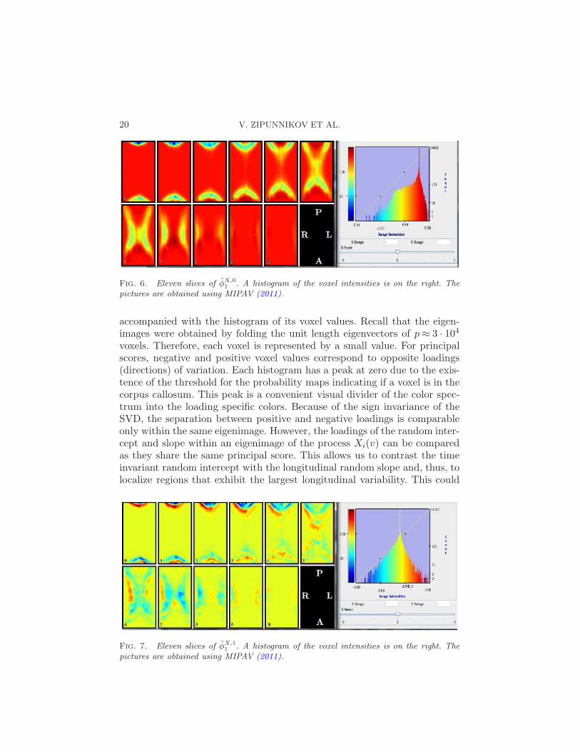
Fig. 6. Eleven slices of φX,01 . A histogram of the voxel intensities is on the right. The

pictures are obtained using MIPAV (2011).

accompanied with the histogram of its voxel values. Recall that the eigen-images were obtained by folding the unit length eigenvectors of p ≈ 3 · 104voxels. Therefore, each voxel is represented by a small value. For principalscores, negative and positive voxel values correspond to opposite loadings(directions) of variation. Each histogram has a peak at zero due to the exis-tence of the threshold for the probability maps indicating if a voxel is in thecorpus callosum. This peak is a convenient visual divider of the color spec-trum into the loading specific colors. Because of the sign invariance of theSVD, the separation between positive and negative loadings is comparableonly within the same eigenimage. However, the loadings of the random inter-cept and slope within an eigenimage of the process Xi(v) can be comparedas they share the same principal score. This allows us to contrast the timeinvariant random intercept with the longitudinal random slope and, thus, tolocalize regions that exhibit the largest longitudinal variability. This could

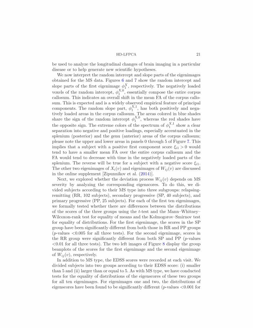
Fig. 7. Eleven slices of φX,11 . A histogram of the voxel intensities is on the right. The

pictures are obtained using MIPAV (2011).

HD-LFPCA 21

be used to analyze the longitudinal changes of brain imaging in a particulardisease or to help generate new scientific hypotheses.

We now interpret the random intercept and slope parts of the eigenimagesobtained for the MS data. Figures 6 and 7 show the random intercept and

slope parts of the first eigenimage φX1 , respectively. The negatively loaded

voxels of the random intercept, φX,01 , essentially compose the entire corpus

callosum. This indicates an overall shift in the mean FA of the corpus callo-sum. This is expected and is a widely observed empirical feature of principalcomponents. The random slope part, φX,1

1 , has both positively and nega-tively loaded areas in the corpus callosum. The areas colored in blue shadesshare the sign of the random intercept φX,0

1 , whereas the red shades have

the opposite sign. The extreme colors of the spectrum of φX,11 show a clear

separation into negative and positive loadings, especially accentuated in thesplenium (posterior) and the genu (anterior) areas of the corpus callosum;please note the upper and lower areas in panels 0 through 5 of Figure 7. Thisimplies that a subject with a positive first component score ξi1 > 0 wouldtend to have a smaller mean FA over the entire corpus callosum and theFA would tend to decrease with time in the negatively loaded parts of thesplenium. The reverse will be true for a subject with a negative score ξi1.The other two eigenimages of Xi(v) and eigenimages of Wij(v) are discussedin the online supplement [Zipunnikov et al. (2014)].

Next, we explored whether the deviation process Wij(v) depends on MSseverity by analyzing the corresponding eigenscores. To do this, we di-vided subjects according to their MS type into three subgroups: relapsing-remitting (RR, 102 subjects), secondary progressive (SP, 40 subjects), andprimary progressive (PP, 25 subjects). For each of the first ten eigenimages,we formally tested whether there are differences between the distributionsof the scores of the three groups using the t-test and the Mann–Whitney–Wilcoxon-rank test for equality of means and the Kolmogorov–Smirnov testfor equality of distributions. For the first eigenimage, the scores in the SPgroup have been significantly different from both those in RR and PP groups(p-values <0.005 for all three tests). For the second eigenimage, scores inthe RR group were significantly different from both SP and PP (p-values<0.01 for all three tests). The two left images of Figure 8 display the groupbeanplots of the scores for the first eigenimage and the second eigenimageof Wij(v), respectively.

In addition to MS type, the EDSS scores were recorded at each visit. Wedivided subjects into two groups according to their EDSS score: (i) smallerthan 5 and (ii) larger than or equal to 5. As with MS type, we have conductedtests for the equality of distributions of the eigenscores of these two groupsfor all ten eigenimages. For eigenimages one and two, the distributions ofeigenscores have been found to be significantly different (p-values <0.001 for

22 V. ZIPUNNIKOV ET AL.

Fig. 8. Model 1: Group beanplots according to MS type (top) and according to EDSSscore (bottom).

all three tests). The two right images on Figure 8 display group beanplotsof the scores for the first eigenimage and the second eigenimage of Wij(v),respectively.

We have also conducted a standard analysis based on the scalar meanFA over the CC for each subject/visit and fitted a scalar random inter-cept/random slope model. In this model, the random intercept explainsroughly 94% of the total variation of the mean FAs. Figure 15 in the onlinesupplement [Zipunnikov et al. (2014)] displays beanplots of the estimatedrandom intercepts stratified by EDDS score and MS type. For both casesthere was a statistically significant difference between the distributions of therandom intercepts (EDSS: p-values < 0.001; MS-type, SP vs. RR and PP,p-values < 0.002, for all three tests). Similar tests for the distributions of therandom slopes did not identify statistically significant differences betweengroups. We conclude that this simple model agrees with the full HD-LFPCAmode, though the multivariate model provides a detailed decomposition ofthe total FA variation together with localization variability in the original3D-space.

HD-LFPCA 23

Table 3

Model 2 (Zij change): Cumulative variability explained by the first 10 eigenimages

k φX,0

k φX,1

k φWk Cumulative

1 17.79 0.42 5.59 23.802 0.53 8.46 1.99 34.783 6.92 0.39 1.55 43.644 4.68 0.76 1.05 50.135 3.02 0.52 0.80 54.466 2.44 0.29 0.69 57.887 1.63 0.77 0.54 60.828 1.48 0.67 0.39 63.369 1.41 0.51 0.35 65.64

10 1.19 0.38 0.33 67.54

41.09 13.17 13.28 67.54

Model 2. Second, we fit model (8) using Zij,1 equal to a visit-specific EDSSscore. Again, Zij,1’s were normalized to have sample mean 0 and sample vari-ance 1. Table 3 reports percentages explained by the first 10 eigenimages inmodel 2. Interestingly, the total variation explained by the random interceptand random slope in both models is approximately the same, with 56.0%in model 1 vs. 54.2% for model 2. However, the random slope in model 2explains a much higher proportion of the total variation: 13.2% in model 2using EDSS versus model 1 using time. The second component of the ran-dom slope explains almost 8.5% of the total variation. We have also exploredwhether the scores of Wij(v) depend on MS type and EDSS score using the t-test, the Mann–Whitney–Wilcoxon-rank test, and the Kolmogorov–Smirnovtest. For the first eigenimage, the SP type was significantly different fromthe RR (p-values < 0.01 for all three tests), though it was not significantlydifferent from the PP group. For the second eigenimage, the distribution ofeigenscores for the SP type was significantly different from that of the scoresfor the RR (p-values < 0.05 for all three tests), and not significantly differentfrom the distribution of the scores of the PP type. For grouping according toEDSS score, the distributions of the eigenscores of the first two eigenimageshave been found to be statistically different (p-values < 0.01 for all threetests). Figure 9 displays beanplots similar to Figure 8 for the distributionsof the scores in the groups defined by MS types and EDSS. This indicatesthat the deviation process Wij(v) in models 1 and 2 carries not only usefulbut also almost identical remaining information regarding severity of MS.

6. Discussion. The methods developed in this paper increase the scopeand general applicability of LFPCA to very high-dimensional settings. Thebase model decomposes the longitudinal data into three main components:

24 V. ZIPUNNIKOV ET AL.

Fig. 9. Model 2: Group beanplots according to MS type (top) and according to EDSSscore (bottom).

a subject-specific random intercept, a subject-specific random slope, and re-versible visit-to-visit deviation. We described and addressed computationaldifficulties that arise with high-dimensional data using a powerful approachreferred to as HD-LFPCA. We have developed a procedure designed to iden-tify a low-dimensional space that contains all the information for estimatingof the model. This significantly extended the previous related efforts in theclustered functional principal components models, MFPCA [Di et al. (2009)]and HD-MFPCA [Zipunnikov et al. (2011a)].

We applied HD-LFPCA to a novel imaging setting considering DTI andMS in a primary white matter structure. Our investigation characterizedlongitudinal and cross-sectional variation in the corpus callosum.

There are several outstanding issues for HD-LFPCA that need to be ad-dressed. First, a key assumption of our methods is that they require a mod-erate sample size that does not exceed ten thousands, or so, images. Thislimitation can be circumvented by adopting the methods discussed in theAppendix. Second, we have not formally included white noise in our model.Simulation studies in Section 4 demonstrated that a moderate amount of

HD-LFPCA 25

white noise does not have a serious effect on the estimation procedure. How-ever, a more systematic treatment of the related issues is required.

In summary, HD-LFPCA provides a powerful conceptual and practi-cal step toward developing estimation methods for structured ultrahigh-dimensional data.

APPENDIX

A.1. Large sample size. The main assumption which has been made inthe paper is that the sample size, n=

∑Ij=1 Ji, is sufficiently small to guar-

antee that calculations of order O(n3) are feasible. Below we briefly describehow our framework can be adapted to settings with many more scans—onthe order of tens or hundreds of thousands.

LFPCA equation (4) models each vector Yij as a linear combination

of columns of matrices ΦX,0, Φ

X,1, ΦW . Assuming that 2NX + NW <

n, each Yij belongs to an at most (2NX + NW )-dimensional linear space

L(ΦX,0,ΦX,1,ΦW ) spanned by those columns. Thus, if model (4) holds ex-

actly the rank of the matrix, Y does not exceed (2NX +NW ) and at most2NX +NW columns of V correspond to nonzero singular values. This im-plies that the intrinsic model (7) can be obtained by projecting onto thefirst 2NX +NW columns of V and the sizes of matrices A

X,0,AX,1,AW in(7) will be (2NX +NW )×NX , (2NX +NW )×NX , and (2NX +NW )×NW ,respectively. Therefore, the most computationally intensive part would re-quire finding the first 2NX +NW left singular vectors of Y. Of course, inpractice, model (4) never holds exactly. Hence, the number of columns ofmatrix V should be chosen to be large enough to either reasonably exceed(2NX +NW ) or to capture the most variability in data. The latter can be es-timated by tracking down the sums of the squares of the corresponding firstsingular vectors. Thus, this provides a constructive way to handle situationswhen n is too large to calculate the SVD of Y.

There are computationally efficient ways to calculate the first k singularvectors of a large matrix. One way is to adapt streaming algorithms [Weng,Zhang and Hwang (2003), Zhao, Yuen and Kwok (2006), Budavari et al.(2009)]. These algorithms usually require only one pass through the data

matrix Y during which information about the first k singular vectors isaccumulated sequentially. Their complexity is of order O(k3p). An alternateapproach is to use iterative power methods [see, e.g., Roweis (1997)]. As thedimension of the intrinsic model, 2NX +NW , is not known in advance, thenumber of left singular vectors to keep and project onto can be adaptively

estimated based on the singular values of the matrix Y. Further developmentin this direction is beyond the scope of this paper.

26 V. ZIPUNNIKOV ET AL.

A.2. Proofs.

Proof of Lemma 1. Using the independence of Yi and Yk, the ex-pectation of pairwise quadratics is

E(Yij1Y′kj2)

(13)

=

ηη′, if k 6= i,

ηη′ +K00X + Tij2K

01X + Tij1K

10X + Tij1Tij2K

11X + δj1j2K

W ,

if i= k,

where δj1j2 is 1 if j1 = j2 and 0 otherwise. From the top equality we getthe MM estimator of the mean, η = n−1

∑i,j Yij . The covariances K

X

and KW can be estimated by de-meaning Yij as Yij = Yij − η and re-

gressing Yij1Y′ij2

on 1, Tij2 , Tij1 , Tij1Tij2 , and δj1j2 . The bottom equality

can be written as E(Yvij1j2

) = Kvfij1j2 , where Y

vij1j2

= Yij2 ⊗ Yij1 is a

p2 × 1 dimensional vector, the parameter of interest is the p2 × 5 matrixK

v = [vec(K00X ),vec(K01

X ),vec(K10X ),vec(K11

X ), vec(KW )], and the covariatesare entries in the 5× 1 vector fij1j2 = (1, Tij2 , Tij1 , Tij1Tij2 , δj1j2)

′. With this

notation EYv =K

vF, where Y

v is p2 ×m dimensional with m=∑I

i=1 J2i

and F is a 5×m dimensional matrix with columns equal to fij1j2 , i= 1, . . . , I

and j1, j2 = 1, . . . , Ji. The MM estimator of Kv is thus Kv = YvF′(FF′)−1,

which provides unbiased estimators of the covariances KX and K

W . If wedenote H=F

′(FF′)−1, we get the result of the lemma. �

Proof of Lemma 2. Let us denote by KXU

and KWU

the matrices de-

fined by equations (5) with S1/2

Uij1U′ij2

S1/2 substituted for Yij1Y

′ij2

. The

2n× 2n dimensional matrix KXU

and the n×n dimensional matrix KWU

are

low-dimensional counterparts of KX and KW , respectively. Using the SVD

representation Yij =VS1/2

Uij , the estimated high-dimensional covariance

matrices can be represented as KX =DK

XUD

′ and KW =VK

WUV

′, wherethe matrix D is 2p× 2n dimensional with orthonormal columns defined as

D=

(V 0p×n

0p×n V

).(14)

From the constructive definition of H, it follows that the matrices KXU

and

KWU

are symmetric. Thus, we can construct their spectral decompositions,

KXU= A

XΛ

XA

X′and K

WU

= AWΛ

WA

W ′. Hence, high-dimensional covari-

ance matrices can be represented as KX = DA

XΛ

XA

X′D

′ and KW =

VAWΛ

WA

W ′V

′, respectively. The result of the lemma now follows fromthe orthonormality of the columns of matrices D and V. �

HD-LFPCA 27

Proof of Lemma 3. With notational changes, the proof is identical tothe proof of Lemma 1. �

Proof of Lemma 4. With notational changes, the proof is identical tothe proof of Lemma 2. �

Proof of Lemma 5. The main idea of the proof is similar to that ofZipunnikov et al. (2011a). We assume that function η(v,Tij) = 0. From themodel it follows that ωi ∼ (0,Λω), where Λω is a covariance matrix of ωi.

When p≤NX + JiNW the BLUP of ωi is given by ωi =Cov(ωi,vec(Yi))×Var(vec(Yi))

−1 vec(Yi) = ΛωB′i(BiΛωB

′i)−1 vec(Yi) [see McCulloch and

Searle (2001), Section 9]. The BLUP is essentially a projection and, thus, itdoes not require any distributional assumptions. It may be defined in termsof a projection matrix. If ξi and ζij are normal, then the BLUP is the bestpredictor. When p > NX + JiNW the matrix BiΛωB

′i is not invertible and

the generalized inverse of BiΛωB′i is used [Harville (1976)]. In that case,

ωi = ΛωB′i(BiΛωB

′i)− vec(Yi) = Λ

1/2ω (Λ

1/2ω B

′iBiΛ

1/2ω )−1

Λ1/2ω B

′i vec(Yi) =

(B′iBi)

−1B

′i vec(Yi). Note that it coincides with the OLS estimator for ωi

if ωi were a fixed parameter. Thus, the estimated BLUPs are given byωi = (B′

iBi)−1

B′i vec(Yi). �

Acknowledgments. The authors would like to thank Jeff Goldsmith forhis help with data management. The content is solely the responsibility of theauthors and does not necessarily represent the official views of the NationalInstitute of Neurological Disorders and Stroke or the National Institute ofBiomedical Imaging and Bioengineering or the National Institutes of Health.

SUPPLEMENTARY MATERIAL

Supplement to “Longitudinal high-dimensional principal components anal-

ysis with application to diffusion tensor imaging of multiple sclerosis” (DOI:10.1214/14-AOAS748SUPP; .pdf). We provide extra figures and tables sum-marizing the results of simulation studies and the analysis of DTI images ofMS patients.

REFERENCES

3D-Slicer (2011). http://www.slicer.org/.Aston, J. A. D., Chiou, J.-M. and Evans, J. P. (2010). Linguistic pitch analysis using

functional principal component mixed effect models. J. R. Stat. Soc. Ser. C. Appl. Stat.59 297–317. MR2744475

Bigelow, J. L. and Dunson, D. B. (2009). Bayesian semiparametric joint models forfunctional predictors. J. Amer. Statist. Assoc. 104 26–36. MR2663031

28 V. ZIPUNNIKOV ET AL.

Budavari, T., Wild, V., Szalay, A. S., Dobos, L. and Yip, C.-W. (2009). Reliableeigenspectra for new generation surveys. Monthly Notices of the Royal AstronomicalSociety 394 1496–1502.

Crainiceanu, C. M., Staicu, A.-M. and Di, C.-Z. (2009). Generalized multilevel func-tional regression. J. Amer. Statist. Assoc. 104 1550–1561. MR2750578

Crainiceanu, C. M., Caffo, B. S., Luo, S., Zipunnikov, V. M. and Punjabi, N. M.

(2011). Population value decomposition, a framework for the analysis of image popula-tions. J. Amer. Statist. Assoc. 106 775–790. MR2894733

Demmel, J. W. (1997). Applied Numerical Linear Algebra. SIAM, Philadelphia, PA.MR1463942

Di, C., Crainiceanu, C. M. and Jank, W. S. (2010). Multilevel sparse functional prin-cipal component analysis. Stat. 3 126–143.

Di, C.-Z., Crainiceanu, C. M., Caffo, B. S. and Punjabi, N. M. (2009). Multilevelfunctional principal component analysis. Ann. Appl. Stat. 3 458–488. MR2668715

Everson, R. and Roberts, S. (2000). Inferring the eigenvalues of covariance matricesfrom limited, noisy data. IEEE Trans. Signal Process. 48 2083–2091. MR1824643

Goldsmith, J., Crainiceanu, C. M., Caffo, B. S. and Reich, D. S. (2011). Penal-ized functional regression analysis of white-matter tract profiles in multiple sclerosis.NeuroImage 57 431–439.

Golub, G. H. and Van Loan, C. F. (1996). Matrix Computations, 3rd ed. Johns HopkinsUniv. Press, Baltimore, MD. MR1417720

Greven, S., Crainiceanu, C., Caffo, B. and Reich, D. (2010). Longitudinal functionalprincipal component analysis. Electron. J. Stat. 4 1022–1054. MR2727452

Guo, W. (2002). Functional mixed effects models. Biometrics 58 121–128. MR1891050Hall, P., Muller, H.-G. and Yao, F. (2008). Modelling sparse generalized longitudinal

observations with latent Gaussian processes. J. R. Stat. Soc. Ser. B Stat. Methodol. 70703–723. MR2523900

Harville, D. (1976). Extension of the Gauss–Markov theorem to include the estimationof random effects. Ann. Statist. 4 384–395. MR0398007

Hua, Z. W., Dunson, D. B., Gilmore, J. H., Styner, M. and Zhu, H. T. (2012).Semiparametric Bayesian local functional models for diffusion tensor tract statistics.NeuroImage 63 460–474.

Karhunen, K. (1947). Uber lineare Methoden in der Wahrscheinlichkeitsrechnung. An-nales Academie Scientiarum Fennicae 37 1–79.

Li, Y., Zhu, H., Shen, D., Lin, W., Gilmore, J. H. and Ibrahim, J. G. (2011). Mul-tiscale adaptive regression models for neuroimaging data. J. R. Stat. Soc. Ser. B Stat.Methodol. 73 559–578. MR2853730

Loeve, M. (1978). Probability Theory II, 4th ed. Springer, New York. MR0651018McCulloch, C. E. and Searle, S. R. (2001). Generalized, Linear, and Mixed Models.

Wiley, New York. MR1884506Minka, T. P. (2000). Automatic choice of dimensionality for PCA. Adv. Neural Inf.

Process. Syst. 13 598–604.MIPAV (2011). http://mipav.cit.nih.gov.Mohamed, A. and Davatzikos, C. (2004). Medical Image Computing and Computer-

Assisted Intervention. Springer, Berlin.Mori, S. (2007). Introduction to Diffusion Tensor Imaging. Elsevier, Amsterdam.Morris, J. S. and Carroll, R. J. (2006). Wavelet-based functional mixed models. J.

R. Stat. Soc. Ser. B Stat. Methodol. 68 179–199. MR2188981Morris, J. S., Baladandayuthapani, V., Herrick, R. C., Sanna, P. and Gut-

stein, H. (2011). Automated analysis of quantitative image data using isomorphic

HD-LFPCA 29

functional mixed models, with application to proteomics data. Ann. Appl. Stat. 5 894–923. MR2840180

Pujol, S. (2010). 3D-Slicer (tutorial). National Alliance for Medical Image Computing(NA-MIC).

Raine, C. S., McFarland, H. and Hohlfeld, R. (2008). Multiple Sclerosis: A Compre-hensive Text. Saunders, Philadelphia, PA.

Reich, D. S., Ozturk, A., Calabresi, P. A. and Mori, S. (2010). Automated vs con-ventional tractography in multiple sclerosis: Variablity and correlation with disability.NeuroImage 49 3047–3056.

Reiss, P. T. and Ogden, R. T. (2008). Functional generalized linear models with appli-cations to neuroimaging. In Poster presentation Workshop on Contemporary Frontiersin High-Dimensional Statistical Data Analysis, Isaac Newton Institute, University ofCambridge, UK.

Reiss, P. T. and Ogden, R. T. (2010). Functional generalized linear models with imagesas predictors. Biometrics 66 61–69. MR2756691

Reiss, P. T., Ogden, R. T., Mann, J. and Parsey, R. V. (2005). Functional logisticregression with PET imaging data: A voxel-level clinical diagnostic tool. Journal ofCerebral Blood Flow & Metabolism 25 s635.

Rodrıguez, A., Dunson, D. B. and Gelfand, A. E. (2009). Bayesian nonpara-metric functional data analysis through density estimation. Biometrika 96 149–162.MR2482141

Roweis, S. (1997). EM algorithms for PCA and SPCA. Adv. Neural Inf. Process. Syst.10 626–632.

Shinohara, R., Crainiceanu, C., Caffo, B., Gaita, M. I. and Reich, D. S. (2011).Population wide model-free quantification of blood-brain-barrier dynamics in multiplesclerosis. NeuroImage 57 1430–1446.

Shou, H., Zipunnikov, V., Crainiceanu, C. and Greven, S. (2013). Structured func-tional principal component analysis. Available at arXiv:1304.6783.

Staicu, A.-M., Crainiceanu, C. M. and Carroll, R. J. (2010). Fast analysis of spa-tially correlated multilevel functional data. Biostatistics 11 177–194.

Weng, J., Zhang, Y. and Hwang, W.-S. (2003). Candid covariance-free incrementalprincipal component analysis. IEEE Transactions on Pattern Analysis and MachineIntelligence 25 1034–1040.

Xiao, L., Ruppert, D., Zipunnikov, V. and Crainiceanu, C. (2013). Fast covarianceestimation for high-dimensional functional data. Available at arXiv:1306.5718.

Yuan, Y., Gilmore, J. H., Geng, X., Styner, M., Chen, K., Wang, J. L. and Zhu, H.

(2014). Fmem: Functional mixed effects modeling for the analysis of longitudinal whitematter tract data. NeuroImage 84 753–764.

Zhao, H.,Yuen, P. C. andKwok, J. T. (2006). A novel incremental principal componentanalysis and its application for face recognition. IEEE Transactions on Systems, Man,and Cybernetics, Part B: Cybernetics 36 873–886.

Zhu, H., Brown, P. J. and Morris, J. S. (2011). Robust, adaptive functional regres-sion in functional mixed model framework. J. Amer. Statist. Assoc. 106 1167–1179.MR2894772

Zipunnikov, V., Caffo, B., Yousem, D. M., Davatzikos, C., Schwartz, B. S. andCrainiceanu, C. (2011a). Multilevel functional principal component analysis for high-dimensional data. J. Comput. Graph. Statist. 20 852–873. MR2878951

Zipunnikov, V., Caffo, B., Yousem, D. M., Davatzikos, C., Schwartz, B. S. andCrainiceanu, C. M. (2011b). Functional principal component models for high dimen-sional brain volumetrics. NeuroImage 58 772–784.

30 V. ZIPUNNIKOV ET AL.

Zipunnikov, V., Greven, S., Shou, H., Caffo, B., Reich, D. S. andCrainiceanu, C. (2014). Supplement to “Longitudinal high-dimensional principal com-ponents analysis with application to diffusion tensor imaging of multiple sclerosis.”DOI:10.1214/14-AOAS748SUPP.

V. Zipunnikov

B. S. Caffo

C. M. Crainiceanu

Department of Biostatistics

Johns Hopkins University

Baltimore, Maryland 21205-2179

USA

E-mail: vzipunn1@jhu.edu

S. Greven

Department of Statistics

Ludwig-Maximilians-University

80539 Munich

Germany

H. Shou

Department of Biostatistics

and Epidemiology

University of Pennsylvania

Philadelphia, Pennsylvania 19104-6021

USA

D. S. Reich

National Institute

of Neurological Disorders and Stroke

National Institutes of Health

Bethesda, Maryland 20824

USA