University of Virginia

RF and Optical Realizations of Chaotic Dynamics

Emeka V. Ikpeazu, Jr.MATH 5250—Dynamical Systems

Professor John ImbrieDecember 3, 2016

Abstract:

Nonlinear systems have a profound characteristics of exhibiting chaos under very specific circumstances. What is more profound is there extraordinary sensitivity to small perturbations in initial conditions. In this paper, I discuss a variety of chaotic systems that show up in electrical engineering applications, particularly in the GHz and THz ranges of the electromagnetic spectrum. These include the Josephson junction and optical chaos. Here, I show that chaos is not only interesting as an effect, but also interesting in the way it can be harnessed in order to realize efficient methods for problems confronting engineers and applied scientists.

1. The Josephson junctionThe Josephson junction is a quantum mechanical device created by sandwiching a

non-superconducting material in between to superconducting devices. This is sort of similar to a superconducting p-n junction, probably more analogous to a p-i-n junction wherein the i-layer an intrinsic absorbing region. The device is named for Welsh physicist Brian Josephson who predicted the tunneling of superconducting electrons through a superconducting device. The device operates at low temperatures where metals become superconductors, usually 20 K or lower. At these sort of temperatures, phase transitions occur in metals and practically diminish any resistance to the flow of electrons in them.

Figure 1.1. The Josephson junction is operated below a certain “critical temperature” so the that the electrons on the opposing sides of the junction exhibit an attractive interaction. This attractive potential creates an energy gap. This energy gap induces a “critical current” across the junction.

When this critical current is exceeded an AC current is created and the phase difference between the two junctionsϕ=ϕ1−ϕ2 is created. The equation for phase

difference in the Josephson junction is written

ϕ=2eℏ V

Figure 1.2. An equivalent circuit is created for the Josephson junction wherein there is a displacement currentC V , a regular currentV / R, and a bias currentI c sin ϕ. In this way

Cℏ2e

ϕ+ ℏ2 eR

ϕ+ I c sin ϕ=I whereℏ is Planck’s constant divided by2π ,

ande is the charge of an electron.

The system can be turned into the following two-dimensional system:

ϕ=2eVℏ V= I

C−

I c sin ϕC

− VRC

However, an additional term can be added to make the

system three-dimensional. It is by coupling the JJ to an RLC circuit wherein the system thereby becomes three-dimensional and chaos is induced [2]. This additional term relates the voltage induced by the inductor of inductance well and that produced by the current

through the resistor of resistanceR. The term relates the voltageV asL I s+ I s Rs=V whereI s is the shunt current. Equivalently, the second equation forV must

be changed to

V=I−I s

C−

I ssin ϕC

− VRC

Via further normalization we get the system [3],

∂ xτ= y∂ yτ=1βc

{i−gy−sin x−z }∂ zτ=y−zβL

wherex=ϕ,y=V /I c R s, andz=I s / I c

. Time is

normalized asτ=ωc t andωc=2 I c R s

ℏ . Voltage is normalized asv=V / I c Rs. There are

other dimensionless parameters such as the normalized capacitance parameterβc=2 Ic Rs

2C /ℏ, the normalized inductance parameterβL=2 e I c L/ℏ, andg=RV / RL.

-100

10

-10

0

10-10

-5

0

5

10

xy

z

_x = 0_y= 0_z = 0

Figure 1.3. The figure above is the phase portrait for an RLC-shunted Josephson junction whereβc=1.08, β l=2.57,i=1.11, andg=0.061.

The Jacobian for this system is written

D FX=J=( 0 1 0−βc

−1 cos x¿ −gβc−1 −βc

−1

0 βL−1 −βL

−1)=( 0 1 0−βc

−1√1−i2 −g βc−1 −βc

−1

0 β L−1 −β L

−1)Accordingly,

the eigenvalues for the Jacobian linearization areλ1=−0.6216+0.9921 iλ2=0.1122−0.5103i λ3=−0.4730−0.4818 i

050

100150

200

-2

0

2

4-0.5

0

0.5

1

1.5

2

xy

z

Figure 1.4. More specifically, a trajectory of the system is shown above where( x0 , y0 , z0 )= (1.5,1 .5,1.8 ).

-50

510

x 10-4

-5

0

5

x 10-4

-2

-1

0

1

2x 10

-4

x y

z

Figure 1.5. Above is plotted the difference in trajectory of two versions of the system in Figure 4 separated by10−4 in each direction for the initial conditions.

Most of the difference is in the x-direction which is plotted below.

0 50 100 150 200 250-4

-2

0

2

4

6

8x 10

-4

x

t

Figure 1.6. Quasiperiodicity in the x-direction takes place where multiple periods appear. The quasi-sinusoidality ofδx (t) shows that the trajectories in the x-direction—and in fact,

all directions—do cross in a semi-periodic interval.

The data above shows the value of Josephson junctions in very high-frequency applications. More interestingly, however, is vacillation of trajectories that are just slightly offset in initial directionality. This can be useful in differential RF amplifiers that rely on detecting phase and frequency differences. Moreover, this behavior allows for a sort of nonlinear heterodyning scheme wherein slightly offset currents and phases can be used to generate quasi-periodic signals an encode information.

2. Optical chaosOptical systems are a different type of dynamical system in regards to chaos. Nonlinear systems like the Lorenz attractor or the Rӧssler system can easily induce chaos under the most standard of initial conditions. Optical chaos is more different; it’s a system whose contributions from nonlinear effects are realized under very intense conditions.

Figure 2.1. Optical chaos begins with this rather simple feedback mechanism with a time delayτ . Here, the laser diode (LD) sends the optical signal through a circulator where it

goes through the system with varying attenuation. This is to decrease the lasing threshold, the amount of gain needed for the steady-state condition [7].

Moreover, this feedback system induces “coherence collapse” as the spectral linewidth broadens via the effects of noise and nonlinear effects [5]. The degree to which the spectral linewidth broadens is a function of the correlation between each cycle in the

feedback system. The electric field induced and the number of carriers in the cavity are a dynamical system described by the Lang-Kobayashi equations:

E=1+iα2

GN n (t ) E (t )+κ e i ωo τ E (t−τ )n=pexc J th−γn (t )−[ Γ+GN n (t ) ]|E (t )|2whereα is the

linewidth enhancement factor,GN is the gain factor,

κ is the coupling between feedback cycles,pexc J th is the injection rate of the carrier pump,

γ is inverse of the lifetimes of the spontaneous carriers,and Γ is the cavity loss.

The second term ofE is blanched to denote that this contribution is extrinsic to the cavity system.

Figure 2.2. The increase in feedback—in this case the parameterκ—leads not only to a spectral broadening, but also to a spectral shift towards a lower frequency.

What is more is that frequency peaks get lost asΔ f fb, the frequency shift induced by feedback coupling, approachesf RO, the relaxation oscillation frequency.

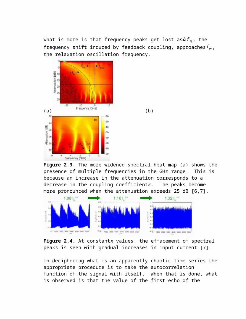
(a) (b)Figure 2.3. The more widened spectral heat map (a) shows the presence of multiple frequencies in the GHz range. This is because an increase in the attenuation corresponds to a decrease in the coupling coefficientκ . The peaks become more pronounced when the attenuation exceeds 25 dB [6,7].

Figure 2.4. At constantκ values, the effacement of spectral peaks is seen with gradual increases in input current [7].

In deciphering what is an apparently chaotic time series the appropriate procedure is to take the autocorrelation function of the signal with itself. When that is done, what is observed is that the value of the first echo of the autocorrelation varies quasi-sinusoidally with the change in the attenuation as seen in Figure 2.5. This pattern was further evinced by doing the same thing with various input photocurrents as shown in Figure 2.6.

Figure 2.5. The maximum correlation Figure 2.6. The maximum correlationhas its first minimum at 18 dB echoes at different photocurrents thatattenuation and its highest around 27.5 are above the threshold photocurrent.dB attenuation [7]. They all exhibit the same pattern [7].

The correlation pattern is explained but parsing the plot into two regimes: a regime of ‘weak chaos’ and one of ‘strong chaos’. The left side has the highest attenuation and thus

the lowest feedback coupling so correlation comes from the high signal to noise ratios which increase with the input photocurrent and thus increase the correlation. On the right

side, bistability takes place in that the laser output has two steady-state equilibrium points. One point is one of chaotic dynamics where feedback cycles experience an

entanglement of sorts and the other is that of stable emission where feedback cycles are more superposed. Optical chaos has many applications when controlled, that is.

Stability analysis in feedback-coupled dynamical systems is similar to that in regular dynamical systems save for that fact that it is sub-Lyapunov exponents that are analyzed instead of Lyapunov exponents [6,7]. In this scheme of analysis, the presence of weak chaos is characterized by negative sub-Lyapunov exponents while that of strong chaos is characterized by positive sub-Lyapunov exponents. Characteristic of coupled

M-ary optical systems is the ansatz Lang-Kobayashi scheme:

x (t )=F [x ( t ) ]+σ∑j=1

M

Gij H [ x ( t−τ ) ]Where G is the coupling matrix normalized to unity.

In both the RF and optical applications of chaos the common requirement for their optimal applicability is control. In the context of non-feedback optical chaos, this comes in the modulation of a parameter, particularly in an oscillatory fashion to achieve an orbit of some sort [8]. In the context of feedback optical chaos vis-à-vis the Lang-Kobayashi system control comes via the continuous application of small perturbations using various methods. The most common of these methods is the OGY (Ott-Grebogi-Yorke) method wherein a cycle is achieved and small kicks are injected to periodically adjust it.

The case of the Josephson junction is also similar although it seems to maintain a rather felicitous autonomous synchrony, much like that of a phase-locked loop as demonstrated in Figure 1.5, thereby eliminating the need for and OGY or Pyragas method of controlling the ensuing chaos in the circuit. In the limit that the applied current I is much less than the critical currentI c and the resistance—assuming this is an RC-shunted JJ—is large the oscillation will carry on for much longer. However, it almost goes without saying that the case of the Josephson junction is one that requires much more similar devices in parallel for any real power to be generated [9]. This, of course, will be facilitated by feedback coupling between these circuits, making the a more complex system, whose dynamical incorrigibility will scale with the power it is expected to generate.

References

1. Shukrinov, Yu.M., Botha, A.E., Medvedeva, S.Yu., Kolahchi, M.R., Irie, A.: Structured chaos in a devil’s staircase of the Josephson junction. Chaos 24, 033115 (2014)

2. Strogatz, S. (1994) Nonlinear Dynamics and Chaos, Addison Wesley Publ.3. Di-Yi Chen, Wei-Li Zhao, Xiao-Yi Ma, and Run-Fan Zhang, “Control and

Synchronization of Chaos in RCL-Shunted Josephson Junction with Noise Disturbance Using Only One Controller Term,” Abstract and Applied Analysis, vol. 2012, Article ID 378457, 14 pages, 2012. doi:10.1155/2012/378457

4. Dana, S.K., Sengupta, D.C., Edoh, K.D.: Chaotic dynamics in Josephson junction. IEEE Trans. Circuit Syst. I 48, 990–996 (2001)

5. T. Heil, I. Fischer, W. Elsäßer, “Coexistence of low-frequency fluctuations and stable emission on a single high-gain mode in semiconductor lasers with external optical feedback,” Physical Review A, 1998

6. S. Heiligenthal, T. Jüngling, O. D’Huys, D. A. Arroyo-Almanza, M. C. Soriano, I. Fischer, I. Kanter, and W. Kinzel, Phys. Rev. E88, 012902 (2013).

7. Xavier Porte, Miguel C. Soriano, and Ingo Fischer, Phys. Rev. A 89, 0238228. L. Illing, D. J. Gauthier, and R. Roy, “Controlling optical chaos, spatio-temporal

dynamics, and patterns,” Adv. Atomic, Molecular, Opt. Phys., vol. 54, pp. 615–697, Mar. 2006.

9. Yu. M. Shukrinov, H. Azemtsa-Donfack and A. E. Botha. Journal: JETP Letters, 2015, Volume 101, Number 4, Page 251